The spine of the $T$-graph of the Hilbert scheme of points in the plane

Abstract.

The torus $T$ of projective space also acts on the Hilbert scheme of subschemes of projective space. The $T$-graph of the Hilbert scheme has vertices the fixed points of this action, and edges connecting pairs of fixed points in the closure of a one-dimensional orbit. In general this graph depends on the underlying field. We construct a subgraph, which we call the spine, of the $T$-graph of $\operatorname{Hilb}^{m}(\mathbb{A}^{2})$ that is independent of the choice of infinite field. For certain edges in the spine we also give a description of the tropical ideal, in the sense of tropical scheme theory, of a general ideal in the edge. This gives a more refined understanding of these edges, and of the tropical stratification of the Hilbert scheme.

1. Introduction

The torus $T\cong(K^{*})^{n}$ of $\mathbb{P}^{n}$ acts on the Hilbert scheme $\operatorname{Hilb}_{P}(\mathbb{P}^{n})$ of subschemes of $\mathbb{P}^{n}$. There are finitely many fixed points of this action, but infinitely many one-dimensional orbits. The $T$-graph of the Hilbert scheme has vertices the fixed points of the $T$-action. There is an edge between two vertices if there is a one-dimensional $T$-orbit containing a $K$-rational point whose closure contains these two vertices. The $T$-graph provides a combinatorial skeleton of the Hilbert scheme; for example, the proof that $\operatorname{Hilb}_{P}(\mathbb{P}^{n})$ is connected given by Peeva and Stillman [PeevaStillman] proceeds by showing the Borel-fixed subgraph of this graph is connected (the original proof by Hartshorne [Hartshorne] has some moves which, while combinatorial, leave this graph). The $T$-graph of the Hilbert scheme was first systematically studied by Altmann-Sturmfels [AltmannSturmfels], who gave an algorithm to compute it using Gröbner bases, and was studied combinatorially by Hering-Maclagan [HeringMaclagan]. More generally, $T$-graphs arise in GKM theory [GKM], where they are used to give a presentation of the equivariant cohomology ring of a variety with $T$-action.

The $T$-graph of the Hilbert scheme $\operatorname{Hilb}^{4}(\mathbb{A}^{2})$ of $4$ points in $\mathbb{A}^{2}$ is shown on the left of Figure 1. Note that a single edge may correspond to multiple one-dimensional $T$-orbits, or even to a positive-dimensional family of them.

Figure 1. The $T$-graph and its spine when $N=4$. The gray curves illustrate the fact that the edge from $\langle{x^{3},xy,y^{2}}\rangle$ to $\langle{x^{2},xy,y^{3}}\rangle$ corresponds to a one-dimensional family of $T$-orbits; taking a limit, the $T$-orbits degenerate into the union of two orbits, corresponding to the edges from $\langle{x^{3},xy,y^{2}}\rangle$ to $\langle{x^{2},y^{2}}\rangle$ and from $\langle{x^{2},y^{2}}\rangle$ to $\langle{x^{2},xy,y^{3}}\rangle$.

An additional complexity is given by the fact that the graph depends on the underlying field; the $T$-graph of $\operatorname{Hilb}^{10}(\mathbb{A}^{2})$ differs for $K=\mathbb{Q}$ and $K=\mathbb{R}$; see [HeringMaclagan]*Example 2.11 and [SilversmithTropicalIdeal]*Theorem 5.11.

The first result of this paper is the construction of a subgraph of the $T$-graph of the Hilbert scheme $\operatorname{Hilb}^{N}(\mathbb{A}^{2})$ that does not depend on the underlying field $K$, provided $K$ is infinite.

A $K$-rational point of $\operatorname{Hilb}^{N}(\mathbb{A}^{2})$ is a subscheme of $\mathbb{A}^{2}$ of length $N$, given by an ideal $I\subseteq S:=K[x,y]$ with $\dim_{K}S/I=N$. Such an ideal $I$ is a fixed point of the $T$-action if and only if it is a monomial ideal; these ideals are in bijection with Young diagrams with $N$ boxes, with boxes corresponding to monomials not in $I$. A non-monomial ideal $I$ lies on a one-dimensional orbit if and only if $I$ is homogeneous with respect to a grading by $\deg(x)=a$ and $\deg(y)=b$; the subscheme of $\mathbb{A}^{2}$ defined by $I$ is stabilized by the subtorus $\{((t^{a},t^{b}):t\in K^{*}\}\subseteq T$. There are two $T$-fixed points in the closure of the orbit, so $I$ corresponds to an edge of the $T$-graph, if and only if $ab>0$.

In this latter case, denote by $h:\mathbb{Z}_{\geq 0}\rightarrow\mathbb{Z}_{\geq 0}$ the Hilbert function of $I$ with respect to this grading: $h(d):=\dim_{K}(S/I)_{d}$. Then $I$ lies on the multigraded Hilbert scheme $\operatorname{Hilb}^{h}_{S}\subseteq\operatorname{Hilb}^{N}(\mathbb{A}^{2})$ parametrizing homogeneous ideals in $S$ with Hilbert function $h$ [HaimanSturmfels]. This multigraded Hilbert scheme is a $T$-invariant closed subscheme of $\operatorname{Hilb}^{N}(\mathbb{A}^{2})$, is smooth and irreducible [Evain]*Theorem 1 [MaclaganSmith]*Theorem 1.1, and has two distinguished $T$-fixed points: the “lex-most” and “lex-least” monomial ideals. See Section 2 and in particular Figure 2 for more details.

Definition 1.1.

The spine $G_{N}^{*}$ of the $T$-graph of $\operatorname{Hilb}^{N}(\mathbb{A}^{2})$ is the graph with vertices the $T$-fixed points of $\operatorname{Hilb}^{N}(\mathbb{A}^{2})$, and an edge between two monomial ideals if they are the lex-most and lex-least ideals of $\operatorname{Hilb}_{S}^{h}$ with respect to some grading and Hilbert function.

Studying the spine was suggested in Remark 4.7 of [HeringMaclagan]. Every one-dimensional $T$-orbit corresponding to an edge of the $T$-graph is in the closure of the set of $T$-orbits corresponding to edges in the spine. The spine for $\operatorname{Hilb}^{4}(\mathbb{A}^{2})$ is shown on the right in Figure 1. Let $G_{N}(K)$ denote the $T$-graph of $\operatorname{Hilb}^{N}(\mathbb{A}^{2})$ over a field $K$. Our first theorem is the following.

Theorem 1.2.

For any infinite field $K$, $G_{N}^{*}$ is a subgraph of $G_{N}(K)$; that is, if $M^{-}$ and $M^{+}$ are the lex-least and lex-most monomial ideals with respect to some grading and Hilbert function, then there exists an ideal $I\subseteq K[x,y]$, homogeneous with respect to this grading and Hilbert function, such that the closure of the $T$-orbit of $I$ contains $M^{-}$ and $M^{+}.$

Our second result, Theorem 1.3 below, refines Theorem 1.2 for some edges by describing matroidal aspects of $\operatorname{Hilb}_{S}^{h}$ coming from tropical scheme theory. We now describe what we mean by this; for precise definitions, see Section 3.1.

The tropicalization $\operatorname{trop}(I)$ of an ideal $I\subseteq K[x,y]$ is the ideal in the semiring of tropical polynomials obtained by tropicalizing every polynomial in the ideal. This is an example of a tropical ideal in the sense of tropical scheme theory [Giansiracusa2, TropicalIdeals, MaclaganRinconValuations, Balancing]. When $I$ is homogeneous, each degree-$d$ part of $\operatorname{trop}(I)$ determines a matroid $\mathcal{M}(I_{d})$ on the set $\mathrm{Mon}_{d}$ of degree-$d$ monomials.

This construction induces a tropical stratification of $\operatorname{Hilb}_{S}^{h}$; two ideals are in the same stratum if and only if their tropicalizations coincide. This can be thought of as a generalization of the matroid stratification of the Grassmannian [GGMS]. Very little is known about the tropical stratification; see [SilversmithTropicalIdeal, FinkGiansiracusaGiansiracusa].

When $n=2$, and the grading is the standard one $\deg(x)=\deg(y)=1$, the Hilbert scheme $\operatorname{Hilb}_{S}^{h}$ is irreducible [Evain, MaclaganSmith], and hence has a unique open (largest) stratum. Our second main theorem, Theorem 1.3 below, describes this stratum; in other words, it describes the tropicalization of a general ideal $I$ in $\operatorname{Hilb}_{S}^{h}.$

Theorem 1.3.

Let $S=K[x,y]$ be graded by $\deg(x)=\deg(y)=1$. For any $d\geq 0$, the degree-$d$ matroid $\mathcal{M}(I_{d})$ of a general ideal $I$ in $\operatorname{Hilb}_{S}^{h}$ is the uniform matroid $U_{h(d),d+1}.$ Furthermore, $I$ can be taken to be a $K$-rational point of $\operatorname{Hilb}_{S}^{h}$, provided $K$ is infinite.

Theorem 1.3 fails in the nonstandard grading; see Section 3.5.

There are comparatively few explicit examples of tropical ideals; see [Zajaczkowska, AndersonRincon]. One important aspect of Theorem 1.3 is thus that it provides a large class of new examples for which all matroids are understood.

Theorem 1.3 refines Theorem 1.2 as follows. For a fixed grading and Hilbert function, the ideals $I\subseteq K[x,y]$ whose orbit contains $M^{-}$ and $M^{+}$ comprise an open set $U_{1}\subseteq\operatorname{Hilb}_{S}^{h}$, which is nonempty by Theorem 1.2. Meanwhile, the ideals $I\subseteq K[x,y]$ such that the conclusion of Theorem 1.3 holds for all $d\geq 0$ also comprise a nonempty open set $U_{2}\subseteq\operatorname{Hilb}_{S}^{h}$, and we have the containment $U_{2}\subseteq U_{1}$; see Remark 3.23.

The structure of this paper is as follows. In Section 2 we give more precise definitions of the main objects of study, and prove Theorem 1.2. Theorem 1.3 is proved in Section 3.

Acknowledgements. Maclagan was partially supported by EPSRC grant EP/R02300X/1. Silversmith was supported by NSF DMS-1645877 and by a Zelevinsky postdoctoral fellowship at Northeastern University. Some background calculations were done using Macaulay2 [M2].

2. The spine of the $T$-graph

In this section we recall previous work on the $T$-graph, and prove Theorem 1.2.

Let $K$ be an infinite field. Recall that a $K$-rational point of $\operatorname{Hilb}^{N}(\mathbb{A}^{2})$ is given by an ideal $I\subseteq S:=K[x,y]$ with $\dim_{K}(S/I)=N$. The $T\cong(K^{*})^{2}$ action on $\mathbb{A}^{2}$ induces a $T$-action on $\operatorname{Hilb}^{N}(\mathbb{A}^{2})$. Such an ideal is a fixed point of the $T\cong(K^{*})^{2}$ action on $\operatorname{Hilb}^{N}(\mathbb{A}^{2})$ if and only if it is a monomial ideal, and lies on a one-dimensional $T$-orbit if and only if it is homogeneous with respect to a $\mathbb{Z}$-grading by $\deg(x)=a$ and $\deg(y)=b$. The closure of a one-dimensional $T$-orbit has either one or two $T$-fixed points; if there are two $T$-fixed points in the closure we have $ab>0$.

Notation 2.1.

We set $S=K[x,y]$. We grade $S$ by $\deg(x)=a$, $\deg(y)=b$, for positive integers $a,b$, and denote this as an $(a,b)$-grading. From now on we restrict to $a,b>0$ and $\gcd(a,b)=1$; this makes no material difference, and will simplify our notation.

Let $I\in\operatorname{Hilb}^{N}(\mathbb{A}^{2})$ be an ideal that is homogeneous with respect to the grading by $(a,b)\in\mathbb{Z}_{>0}^{2}$. The Hilbert function $h:\mathbb{Z}_{\geq 0}\to\mathbb{Z}_{\geq 0}$ of $I$ is defined by $h(d)=\dim_{K}(S/I)_{d}.$ Note that $\sum_{d\geq 0}h(d)=N.$ The point $I\in\operatorname{Hilb}^{N}(\mathbb{A}^{2})$ is contained in the closed subscheme $\operatorname{Hilb}_{S}^{h}$ parametrizing ideals in $S$ that are homogeneous with respect to the $(a,b)$-grading and have Hilbert function $h$. This subscheme is a multigraded Hilbert scheme in the sense of [HaimanSturmfels]. Furthermore, for any grading $(a,b)\in\mathbb{Z}_{>0}^{2}$ and for any Hilbert function $h:\mathbb{Z}_{\geq 0}\to\mathbb{Z}_{\geq 0}$ with $\sum_{d\geq 0}h(d)=N,$ if the scheme $\operatorname{Hilb}_{S}^{h}$ is nonempty, it is a smooth irreducible $T$-invariant subvariety of $\operatorname{Hilb}^{N}(\mathbb{A}^{2})$ [Evain, MaclaganSmith]. The union of the subvarieties $\operatorname{Hilb}_{S}^{h}$, as $(a,b)$ and $h$ vary, is precisely the set of ideals corresponding to vertices and edges of the $T$-graph, and any intersection of two different $\operatorname{Hilb}_{S}^{h}$ is either empty, or consists of a single point corresponding to a monomial ideal.

Each multigraded Hilbert scheme $\operatorname{Hilb}_{S}^{h}$ inherits a $T$-action from $\operatorname{Hilb}^{N}(\mathbb{A}^{2}).$ We may define the $T$-graph $G_{h}(K)$ of $\operatorname{Hilb}_{S}^{h}$ in exact analogy with that of $\operatorname{Hilb}^{N}(\mathbb{A}^{2})$: the vertices of $G_{h}(K)$ are zero-dimensional $T$-orbits, which are monomial ideals whose Hilbert function with respect to $(a,b)$ is $h$, and two vertices are connected by an edge if there is a one-dimensional $T$-orbit in $\operatorname{Hilb}_{S}^{h}$ containing a $K$-rational point whose closure contains those vertices. Note that $G_{h}(K)$ is naturally a subgraph of $G_{N}(K)$. Moreover, we have the following decomposition:

Proposition 2.2 ([HeringMaclagan], Corollary 2.6).

The $T$-graph $G_{N}(K)$ is the union of the subgraphs $G_{h}(K)$ as $(a,b)$ and $h$ vary, and these subgraphs have disjoint edge sets.

In light of Proposition 2.2, in order to determine $G_{N}(K)$ it is sufficient to study the graded Hilbert schemes $\operatorname{Hilb}_{S}^{h}$ separately. Thus from now on, fix a grading $(a,b)\in\mathbb{Z}_{>0}^{2}$ with $\gcd(a,b)=1$, and a Hilbert function $h:\mathbb{Z}_{\geq 0}\to\mathbb{Z}_{\geq 0}$ with $\sum_{d\geq 0}h(d)<\infty.$

Note that the 1-parameter subtorus $T_{a,b}:=\{(t^{a},t^{b})\thickspace|\thickspace t\in K^{*}\}\subseteq T$ acts trivially on $\operatorname{Hilb}_{S}^{h}$, so we need only consider the action of the one-dimensional torus $T/T_{a,b}$. Since $\operatorname{Hilb}_{S}^{h}$ is smooth and projective, the Białynicki-Birula decomposition of $\operatorname{Hilb}_{S}^{h}$ with respect to $T/T_{a,b}$ decomposes $\operatorname{Hilb}_{S}^{h}$ as a union of affine spaces, each consisting of points whose limit under the subtorus action is a given fixed point. We describe these affine spaces algebraically as follows. Set $\prec$ to be the lexicographic order with $x\prec y$. A $T$-fixed point corresponds to a monomial ideal $M$. The Białynicki-Birula cell associated to $M$ is

$$C_{\prec}(M)=\{I\in\operatorname{Hilb}_{S}^{h}\thickspace|\thickspace\operatorname{in}_{\prec}(I)=M\},$$

where $\operatorname{in}_{\prec}(I)$ is the initial ideal in the sense of Gröbner bases; see [CLO]. An explicit parameterization of $C_{\prec}(M)$ was given by Evain [Evain]; we recall this in Section 3.2. For two monomial ideals $M,M^{\prime}\in\operatorname{Hilb}_{S}^{h}$, the edge-scheme between $M$ and $M^{\prime}$ is the scheme-theoretic intersection

$$E(M,M^{\prime})=C_{\prec}(M)\cap C_{\prec^{opp}}(M^{\prime}),$$

where $\prec^{opp}$ is the lexicographic order with $x\succ y$. This was first studied computationally by Altmann and Sturmfels [AltmannSturmfels]. There is an edge between $M$ and $M^{\prime}$ in the $T$-graph if and only if one of $E(M,M^{\prime})$ and $E(M^{\prime},M)$ has a $K$-rational point.

The vertices of $G_{N}(K)$ are purely combinatorial: colength-$N$ monomial ideals in $S=K[x,y]$ correspond to partitions of $N$, and requiring that the Hilbert function with respect to $(a,b)$ is $h$ is a combinatorial condition on partitions of $N=\sum_{d\geq 0}h(d)$. The edges, however, depend on the field $K$, as the following examples show.

Example 2.3.

There is an edge between the two monomial ideals $M=\langle x^{5},y^{2}\rangle$ and $M^{\prime}=\langle x^{2},y^{5}\rangle$ when viewed as ideals in $\mathbb{R}[x,y]$, but not when viewed as ideals in $\mathbb{Q}[x,y]$, so the $T$-graph of $\operatorname{Hilb}^{10}(\mathbb{A}^{2})$ differs over $\mathbb{R}$ and ${\mathbb{Q}}$. This is the case because every ideal in $E(M,M^{\prime})$ has the form $I=\langle y^{2}+\alpha xy+\beta x^{2},x^{5}\rangle$, with $\alpha^{4}-3\alpha^{2}\beta+\beta^{2}=0$, by [HeringMaclagan]*Example 2.11. This is the union of two one-dimensional $T$-orbits, which have $\mathbb{R}$-rational points, but no $\mathbb{Q}$-rational points. Note that the edge scheme $E(M,M^{\prime})$ is a subscheme of $\operatorname{Hilb}_{S}^{h}$, where the grading is $(1,1),$ and $h=(1,2,2,2,2,1,0,0,\ldots).$

This example is generalized in [SilversmithTropicalIdeal]*Theorem 5.11, which shows that if $m>k>0,$ and we define $M=\langle x^{m},y^{k}\rangle$ and $M^{\prime}=\langle x^{k},y^{m}\rangle$ in $\operatorname{Hilb}^{mk}(\mathbb{A}^{2})$, then the edge-scheme $E(M,M^{\prime})$ is one dimensional and reducible over $\mathbb{C}$, with the number of irreducible components equal to the number of binary necklaces with $k$ black and $m-k$ white beads. The proof actually shows that these edges have $K$-rational points whenever there exists $c\in K$ such that $x^{m}+cy^{m}$ has a degree-$k$ factor with coefficients in $K$.

By contrast, the definition of the spine of the $T$-graph, given in Definition 1.1, is purely combinatorial.

Definition 2.4.

Let $M,M^{\prime}$ be monomial ideals in $\operatorname{Hilb}_{S}^{h}$. We define $M\preceq M^{\prime}$ if for each degree $d$ there is a degree-preserving bijection $f$ from the monomials in $M$ to the monomials in $M^{\prime}$ with $m\succeq f(m)$ for all monomials $m\in M$, where $\prec$ is the lexicographic order with $x\prec y$. This defines a partial ordering on the monomial ideals in $\operatorname{Hilb}_{S}^{h}$.

Remark 2.5.

The partial order of Definition 2.4 may be regarded as a graded version of the dominance order for partitions. Recall that the monomial ideals $M,M^{\prime}$ correspond to partitions, or alternatively, to Young diagrams. Under this correspondence, $M\preceq M^{\prime}$ if and only if $M^{\prime}$ can be obtained from $M$ by moving boxes of the Young diagram up and to the left, along lines of slope $-a/b.$ See Figure 2. Compare this to the usual dominance order for partitions, which is identical after removing the slope restriction.

A necessary, but not sufficient, condition for $E(M,M^{\prime})$ to be nonempty is that $M\preceq M^{\prime}$ with respect to this partial order; this is a straightforward special case of [HeringMaclagan, Thm. 1.3]. In particular, if $M\neq M^{\prime},$ then at most one of $E(M,M^{\prime})$ and $E(M^{\prime},M)$ is nonempty. We may therefore regard $G_{N}(K)$ as a directed graph, with an edge from $M$ to $M^{\prime}$ if $E(M,M^{\prime})$ is nonempty; the necessary condition above implies that the resulting directed graph is acyclic.

Figure 2. The poset of monomial ideals in $\operatorname{Hilb}^{h}_{S}$, where $h=(1,1,2,1,1,0,0,\ldots)$ with respect to the $(1,2)$-grading. The leftmost ideal is the lex-least, and the rightmost ideal is the lex-most. Note that $M_{1}\prec M_{2}$ if and only if $M_{2}$ can be obtained from $M_{1}$ by moving boxes of the Young diagram up-and-left along lines of slope $-1/2$.

It was first noted by Evain [Evain]*Theorem 19 that this poset has a unique maximal element, which we denote by $M^{+}$, and a unique minimal element, which we denote by $M^{-}$; see also [MaclaganSmith]*Proposition 3.12. We call $M^{+}$ the lex-most ideal with Hilbert function $h$, and $M^{-}$ the lex-least such ideal.

As defined in Definition 1.1, the spine $G^{*}_{N}$ of the $T$-graph of $\operatorname{Hilb}^{N}(\mathbb{A}^{2})$ is the graph with vertices monomial ideals $M$ in $S$ with $\dim_{K}(S/M)=N$, and an edge joining two ideals $M,M^{\prime}$ if $M=M^{-}$, and $M^{\prime}=M^{+}$ for some grading $(a,b)$ and Hilbert function. Figure 3 shows $G_{6}(\mathbb{C})$ and $G_{6}^{*}$.

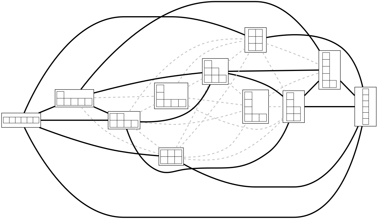
Figure 3. The $T$-graph $G_{6}(\mathbb{C})$, where the edges of $G_{6}^{*}$ are solid.

Theorem 2.6.

Let $K$ be an infinite field. If there is an edge connecting two monomial ideals $M,M^{\prime}$ in $G^{*}_{N}$, then there is an edge in the $T$-graph $G_{N}(K)$ connecting $M,M^{\prime}$.

Proof.

Suppose $M$ and $M^{\prime}$ are connected by an edge in $G^{*}_{N}.$ By definition, there exists a grading $(a,b)$ with respect to which the Hilbert functions of $M$ and $M^{\prime}$ agree, and after possibly renaming $M$ and $M^{\prime}$, we have $M=M^{+}$ and $M^{\prime}=M^{-}.$

By [Evain, Thm. 1], [MaclaganSmith, Thm. 1.1], $\operatorname{Hilb}_{S}^{h}$ is smooth, projective, and irreducible. Since $M^{+}$ is a source, and $M^{-}$ is a sink, of the $T/T_{a,b}$ action, the Białynicki-Birula cells $C_{\prec^{opp}}(M^{+})$ and $C_{\prec}(M^{-})$ are Zariski open and isomorphic to affine spaces ([BialynickiBirula],[Evain, Thm. 11]). Note that this follows from [BialynickiBirula] only when the field $K$ is algebraically closed, but this assumption is unnecessary — for a discussion see [Brosnan, §3]. Also, while [Evain] assumes $K$ is algebraically closed, this is never used in the proofs. Thus $C_{\prec^{opp}}(M^{+})\cap C_{\prec}(M^{-})$ is isomorphic to an open subset of an affine space over $K$; since $K$ is infinite, it follows that $C_{\prec^{opp}}(M^{+})\cap C_{\prec}(M^{-})$ contains a $K$-rational point. ∎

3. The tropical ideal of an edge of the spine

In this section we prove Theorem 1.3.

3.1. Tropicalizations of ideals

We first recall the concept of tropicalization of ideals, and the tropical stratification of the Hilbert scheme.

Let $\mathbb{B}=(\{0,\infty\},\mathrel{\oplus},\hskip 1.13809pt{\mathchoice{{\ooalign{$\displaystyle\circ$\cr\hfil$\displaystyle\cdot$\hfil\cr}}}{{\ooalign{$\textstyle\circ$\cr\hfil$\textstyle\cdot$\hfil\cr}}}{{\ooalign{$\scriptstyle\circ$\cr\hfil$\scriptstyle\cdot$\hfil\cr}}}{{\ooalign{$\scriptscriptstyle\circ$\cr\hfil$\scriptscriptstyle\cdot$\hfil\cr}}}}\hskip 1.13809pt)$ be the Boolean semiring, with the operations of tropical addition (minimum) and tropical multiplication (addition). The tropicalization of $f=\sum c_{ij}x^{i}y^{j}\in K[x,y]$ is $\operatorname{trop}(f)=\mathrel{\oplus}_{c_{ij}\neq 0}x^{i}y^{j}\in\mathbb{B}[x,y]$. The tropicalization of an ideal $I\subseteq K[x,y]$ is

$$\operatorname{trop}(I)=\langle\operatorname{trop}(f):f\in I\rangle\subseteq\mathbb{B}[x,y].$$

This is the trivial valuation case of tropicalizing ideals in the sense of tropical scheme theory [Giansiracusa2, TropicalIdeals, MaclaganRinconValuations, Balancing].

Note that a polynomial in the semiring $\mathbb{B}[x,y]$ can be identified with its support. When $I\subseteq S$ is graded, the polynomials in $\operatorname{trop}(I)$ of degree $d$ of minimal support are the circuits of a matroid $\mathcal{M}(I_{d})$ on the ground set $\mathrm{Mon}_{d}$ of degree-$d$ monomials. We call this the degree-$d$ matroid of $I$. See, for example, [Oxley] for more on matroids.

We will primarily focus on the basis characterization of matroids. When $I\subseteq S$ is homogeneous with Hilbert function $h$, a collection $E$ of $h(d)$ monomials of degree $d$ is a basis for $\mathcal{M}(I_{d})$ if there is no polynomial in $I$ with support in $E$. The matroid $\mathcal{M}(I_{d})$ is uniform if every collection of $h(d)$ monomials of degree $d$ is a basis. In this case we write $\mathcal{M}(I_{d})=U_{h(d),\mathrm{mon}_{d}}$, where $\mathrm{mon}_{d}=|\mathrm{Mon}_{d}|$.

The assignment $I\mapsto\operatorname{trop}(I)$ defines a stratification of $\operatorname{Hilb}_{S}^{h}$, called the matroid stratification or tropical stratification. A stratum of this stratification consists of all ideals with a fixed tropicalization. If $\sum_{d}h(d)<\infty$ (as will always be true in this paper), then there are finitely many strata, and they are Zariski-locally closed. In general, there may be countably many strata; see [SilversmithTropicalIdeal].

3.2. Evain’s parameterization of the Białynicki-Birula cells

In this section we recall Evain’s parameterization of the Białynicki-Birula cells. This relies on the combinatorial decomposition of the tangent space to the Hilbert scheme at a monomial ideal given by significant arrows.

Notation 3.1.

Let $\prec$ denote the lexicographic order on monomials in $S=K[x,y]$ with $x\prec y$. We set $r$ to be the Laurent monomial $x^{b}/y^{a}$. When $(a,b)=(1,1)$, we have $r=x/y$.

Definition 3.2.

Let $M\subseteq S$ be a finite-colength monomial ideal. Write the minimal generators for $M$ as $m_{0}\prec m_{1}\prec\dots\prec m_{e}$, so $m_{0}$ is a power of $x$, and $m_{e}$ is a power of $y$. For $1\leq i\leq e$ set $w_{i}=\operatorname{lcm}(m_{i},m_{i-1})$.

The set $T^{+}(M)$ is

$$T^{+}(M)=\{(i,\ell):1\leq i\leq e,\ell\in\mathbb{Z}_{\geq 1},m_{i}r^{\ell}\in S\setminus M,w_{i}r^{\ell}\in M\}.$$

Elements of $T^{+}(M)$ are often drawn as arrows from $m_{i}$ to $m_{i}r^{\ell}$, and are called positive significant arrows. This is illustrated in Figure 4.

The set $T^{-}(M)$ of negative significant arrows has arrows pointing in the other direction:

$$T^{-}(M)=\{(i,\ell):0\leq i\leq e-1,\ell\in\mathbb{Z}_{\leq-1},m_{i}r^{\ell}\in S\setminus M,w_{i+1}r^{\ell}\in M\}.$$

Figure 4. The ideal $M=\langle{x^{11},x^{8}y,x^{4}y^{2},xy^{3},y^{7}}\rangle$ has $T^{+}(M)=\{(1,1),(2,1),(2,2),(3,1),(3,2)\}$ with respect to the grading $(1,2).$

Remark 3.3.

The use of arrows as a combinatorial basis for the tangent space of the Hilbert scheme of points at a monomial ideal was introduced by Haiman in [HaimanQTCatalan]. In Haiman’s formulation there is an equivalence class of arrows; we follow the convention introduced in [Evain] to choose a particular representative of this class that starts at a minimal generator of the ideal, and use the notation from [MaclaganSmith].

The lex-most and lex-least ideals $M^{+}$ and $M^{-}$ defined in Section 2 can be characterized as the unique ideals with $T^{+}(M^{+})=T^{-}(M^{-})=\emptyset$. This was first shown in [Evain], and generalized in [MaclaganSmith].

We next recall the construction of the universal ideal over $C_{\prec}(M)$.

Definition 3.4.

For a monomial $m\in M,$ we define

$$j^{+}(m) =\max\{i\thickspace|\thickspace\text{$m_{i}$ divides $m$}\},\text{ and }$$

$$j^{-}(m) =\min\{i\thickspace|\thickspace\text{$m_{i}$ divides $m$}\}.$$

Note $j^{+}$ is denoted by $j$ in [HeringMaclagan]. We form the polynomial ring $K[\{c_{i}^{\ell}\thickspace|\thickspace(i,\ell)\in T^{+}(M)\}]$ with variables indexed by $T^{+}(M)$, and recursively define polynomials

$$f_{0},\ldots,f_{e}\in K[\{c_{i}^{\ell}\thickspace|\thickspace(i,\ell)\in T^{+}(M)\}][x,y]$$

by $f_{0}=m_{0}$ and

$$f_{i}=\frac{m_{i}}{m_{i-1}}f_{i-1}+\sum_{(i,\ell)\in T^{+}(M)}c_{i}^{\ell}\frac{m_{i}r^{\ell}}{m_{j^{+}(w_{i}r^{\ell})}}f_{j^{+}(w_{i}r^{\ell})}.$$

Note that the initial (leading) term of $f_{i}$ with respect to $\prec$ is $m_{i}$.

Theorem 3.5 ([Evain], Theorem 11).

The set $\{f_{0},\ldots,f_{e}\}$ is a Gröbner basis for the universal ideal $I$ over $C_{\prec}(M)$. The induced map $\mathbb{A}^{\left\lvert T^{+}(M)\right\rvert}\to H_{S}^{h}$ is injective with image $C_{\prec}(M).$

We will work directly with the coefficients of $f_{i}$. To do so, we will use a combinatorial non-recursive description of these coefficients given in [HeringMaclagan], which we now describe.

Definition 3.6 ([HeringMaclagan]*Definition 4.10).

A path from a generator $m_{i}\in M$ is a sequence of positive significant arrows $P=((i_{1},\ell_{1}),(i_{2},\ell_{2}),\ldots,(i_{d},\ell_{d}))$, such that:

1. $i_{1}\leq i,$ and

2. if $d\geq 2,$ then $((i_{2},\ell_{2}),\ldots,(i_{d},\ell_{d}))$ is a path from $m_{j^{+}(w_{i_{1}}r^{\ell_{1}})}$.

The length of $P$ is $l(P)=\ell_{1}+\cdots+\ell_{d}.$ We also associate to $P$ the monomial $c_{P}=c_{i_{1}}^{\ell_{1}}\cdots c_{i_{d}}^{\ell_{d}}$ in $K[C_{\prec}(M)]=K[c_{i}^{\ell}:(i,\ell)\in T^{+}(M)]$. If the sequence is empty, $P$ is the empty path, which has length $0$, and $c_{P}=1$.

Example 3.7.

In Figure 4, the paths from $m_{3}$ are as follows:

Length	Paths
1	((3,1)), ((2,1)), ((1,1))
2	((3,2)), ((3,1),(2,1)), ((3,1),(1,1)), ((2,2)), ((2,1),(1,1))
3	((3,2),(1,1)), ((3,1),(2,2)), ((3,1),(2,1),(1,1))

The boldfaced paths are the direct paths, defined in Definition 3.10.

Theorem 3.8 ([HeringMaclagan], Lemma 4.12).

We have the following alternate characterization of $f_{i}$:

$$f_{i}=\sum_{\begin{subarray}{c}\text{$P$ a path }\\ \text{from $m_{i}$}\end{subarray}}c_{P}m_{i}r^{l(P)}.$$

Note that the term in this sum corresponding to the empty path is $m_{i}$.

Example 3.9.

Continuing Example 3.7, we have $f_{0}=m_{0}=x^{11}$, $f_{1}=x^{8}y+c_{1}^{1}x^{10}$, $f_{2}=x^{4}y^{2}+(c_{1}^{1}+c_{2}^{1})x^{6}y+(c_{2}^{1}c_{1}^{1}+c_{2}^{2})x^{8}$, and $f_{3}=xy^{3}+(c_{1}^{1}+c_{2}^{1}+\mathbf{c_{3}^{1}})x^{3}y^{2}+(c_{2}^{1}c_{1}^{1}+c_{2}^{2}+c_{3}^{1}c_{1}^{1}+c_{3}^{1}c_{2}^{1}+\mathbf{c_{3}^{2}})x^{5}y+(c_{3}^{1}c_{2}^{1}c_{1}^{1}+c_{3}^{1}c_{2}^{2}+\mathbf{c_{3}^{2}c_{1}^{1}})x^{7}$. The boldfaced monomials $c_{P}$ correspond to direct paths, defined in Definition 3.10.

We will focus on one monomial $c_{P}$ in each term of $f_{i}$, as follows.

Definition 3.10.

Fix $k\geq 1$. For all $j\leq k$, let $\ell_{j}$ be the longest length of a significant arrow $(j,\ell^{\prime})\in T^{+}(M^{-})$. We construct a sequence $(z_{1},z_{2},\dots)$ of variables $c_{i}^{\ell^{\prime}}$ as follows. Set $m=m_{k}$, and $l=1$. If $\ell_{k}>0$, set $z_{1}=c_{k}^{\ell_{k}}$, $i=j^{+}(w_{k}r^{\ell_{k}})$, and $l=2$. Otherwise set $i=k-1$. We now iterate. Given $m,l,i$, if $\ell_{i}>0$, set $z_{l}=c_{i}^{\ell_{i}}$, $i=j^{+}(w_{i}r^{\ell_{i}})$, and $l=l+1$. Otherwise set $i=i-1$. This procedure stops when $i\leq 0$.

A path $P$ is called a direct path from $m_{k}$ if it is of one of the two forms $(z_{1},z_{2},\ldots,z_{s})$, with $s>0$, or $(z_{1},z_{2},\ldots,z_{s},c_{i^{\prime}}^{\ell^{\prime}})$, with $s\geq 0$, where the index $i^{\prime}$ agrees with the index of $z_{s+1}$, and $\ell^{\prime}<\ell_{i^{\prime}}$.

Remark 3.11.

Note the following properties:

1. There is at most one direct path from $m_{k}$ of a given length $\ell$. This is because a choice of path is determined by $s$ and $\ell^{\prime}$, and the corresponding path has length $\ell=\sum_{i=1}^{s}\ell_{i}+\ell^{\prime}<\sum_{i=1}^{s+1}\ell_{i}$. We refer to this path, when it exists, as $p_{k,\ell}$.

2. For a fixed $k,$ and a fixed positive significant arrow $c_{i}^{\ell^{\prime}},$ there is at most one $\ell$ such that $c_{i}^{\ell^{\prime}}$ is the last step in a direct path $p_{k,\ell}$, in the sense that for any other positive significant arrow $c_{i^{\prime}}^{\ell^{\prime\prime}}$ in $p_{k,\ell},$ we have $i^{\prime}>i.$

3. If $P$ is a direct path from $m_{k}$ of length $\ell>\ell_{k}$, then the path $P^{\prime}$ obtained by deleting the first step of $P$ is a direct path of length $\ell-\ell_{k}$ from $m_{j^{+}(w_{k}r^{\ell_{k}})}.$

When $S$ has the standard grading, we next show that direct paths of all possible lengths exist from certain monomials $m_{k}$. This uses the following properties of the lex-most and lex-least ideals.

Remark 3.12.

In the standard grading $\deg(x)=\deg(y)=1,$ the lex-most ideal $M^{+}$ is the lexicographic ideal, also known as the lexsegment ideal, with respect to the order $x\succ y$; see [BrunsHerzog]*Chapter 4. This is the monomial ideal whose degree $d$ part is the span of the $(d+1)-h(d)$ largest monomials in lexicographic order. The lex-least ideal $M^{-}$ is the lexicographic ideal for the opposite order of the variables $x\prec y$. A monomial ideal is lex-least with respect to the standard grading if and only if the rows of its Young diagram are strictly decreasing in length, and similarly is lex-most if and only if the columns of its Young diagram are strictly decreasing in length. This means that for $M^{-}$ we have $m_{k}=x^{i}y^{k}$ for some $i$, so $m_{k}r^{\ell}\in S$ for $0\leq\ell\leq k$. We also have by symmetry that if $M^{-}$ and $M^{+}$ are the lex-least and lex-most monomial ideals with a given Hilbert function $h$ respectively, then the Young diagrams of $M^{-}$ and $M^{+}$ are transposes of each other.

Another standard-graded fact about $M^{-}$ that we need, which is not true for nonstandard gradings, is that $w_{k}/m_{k-1}=y$ for all $k\geq 1$.

Proposition 3.13.

Fix the standard $(1,1)$-grading for $S$. Fix $k\geq 0$ with $m_{k}r\in S\setminus M^{-}$. If for some $0<\ell\leq k$ we have that $m_{k}r^{\ell}\in S\setminus M^{-}$, then there is a direct path of length $\ell$ from $m_{k}$.

Proof.

The proof is by induction on $k$. When $k=0$, there is no such $\ell$, so the claim holds. Now assume that the claim is true for all $k^{\prime}<k$. Let $\ell^{\prime}$ be maximal such that $(k,\ell^{\prime})\in T^{+}(M^{-})$. If $\ell^{\prime}\geq\ell$, then we claim that $(k,\ell)\in T^{+}(M^{-})$. This follows from the fact that $w_{k}r^{\ell^{\prime}}\in M^{-}$, so since $w_{k}r^{\ell^{\prime}}\preceq w_{k}r^{\ell}$, we have $w_{k}r^{\ell}\in M^{-}$. In this case $c_{k}^{\ell}$ is the required direct path. Otherwise, $(k,\ell)\not\in T^{+}(M^{-})$, so $w_{k}r^{\ell}\in S\setminus M^{-}$. Let $k^{\prime}=j^{+}(w_{k}r^{\ell^{\prime}})=k-\ell^{\prime}$. We have $w_{k}r^{\ell^{\prime}}=x^{i}m_{k^{\prime}}$ for some $i\geq 0$. Thus $m_{k^{\prime}}r^{\ell-\ell^{\prime}}x^{i}=w_{k}r^{\ell}$, so since $w_{k}r^{\ell}\in S\setminus M^{-}$, the same is true for $m_{k^{\prime}}r^{\ell-\ell^{\prime}}$, and $\ell-\ell^{\prime}\leq k^{\prime}$. Since $\ell^{\prime}<\ell\leq k$, we have $k^{\prime}>1$ and $\ell^{\prime}+1\leq k$. This means that $w_{k}r^{\ell^{\prime}+1}\in S$, and $m_{k^{\prime}}r\in S\setminus M^{-}$, as otherwise we would have $m_{k^{\prime}}x^{i}r=w_{k}r^{\ell^{\prime}+1}\in M^{-}$, so $(k,\ell^{\prime}+1)$ would be in $T^{+}(M^{-})$. By induction there is a direct path $c_{P}$ from $m_{k^{\prime}}$ of length $\ell-\ell^{\prime}$, so $c_{k}^{\ell^{\prime}}c_{P}$ is a direct path of length $\ell$ from $m_{k}$. ∎

3.3. The structure of the Macaulay matrix

For the rest of this section, we fix the standard $(1,1)$ grading on $S=K[x,y]$, and a Hilbert function $h:\mathbb{Z}_{\geq 0}\to\mathbb{Z}_{\geq 0}.$ Let $I\subseteq K[c_{i}^{\ell}:(i,\ell)\in T^{+}(M^{-})][x,y]$ be the ideal of the universal family over $C_{\prec}(M^{-})$ as in Theorem 3.5. Note that there are $\mathrm{mon}_{d}=d+1$ monomials of degree $d$ in $S$.

For any $d\geq 0$, and for any basis of $I_{d}$, we may write the coefficients of the basis as the columns of a matrix $R$ with entries in $K[C_{\prec}(M^{-})]$; such a matrix is called a degree-$d$ Macaulay matrix for $I$, and has size $(d+1)\times(d+1-h(d))$. For any collection $E$ of $h(d)$ monomials of degree $d$, there is a polynomial in $I$ with support in $E$ if and only if the minor indexed by rows corresponding to monomials not in $E$ is zero. The matroid $\mathcal{M}(I_{d})$ is thus exactly characterized by which maximal minors of $R$ vanish.

We begin by choosing a basis for $I_{d}$ via the combinatorial set-up given in Section 3.2. For each of the $d+1-h(d)$ monomials $m\in M^{-}_{d}$, the polynomial $g_{m}:=\frac{m}{m_{j^{-}(m)}}f_{j^{-}(m)}\in I_{d}$ has initial term $m$ with respect to $x\prec y$.

As the polynomials $\{g_{m}\}_{m\in M^{-}_{d}}$ have distinct initial terms, they are all linearly independent. Since $\dim(I_{d})=d+1-h(d)=\left\lvert M^{-}_{d}\right\rvert,$ we conclude that $\{g_{m}\}_{m\in M^{-}_{d}}$ is a basis for $I_{d}.$

Let $R$ be the matrix with columns the coefficient vectors of the polynomials $g_{m}$. This is a degree-$d$ Macaulay matrix for $I$. We index the rows by $\mathrm{Mon}_{d}$ in increasing order with respect to $x\prec y$, and index the columns by the monomials in $M^{-}_{d}$ in increasing order with respect to $x\prec y$, so $R_{m^{\prime},m}$ is the coefficient of $m^{\prime}$ in $g_{m}.$

We now make a series of observations about the matrix $R$.

Property 3.14.

The matrix $R$ is upper triangular in the following sense. If $m^{\prime}\succ m,$ then $R_{m^{\prime},m}=0$ as $g_{m}$ has initial term $m$. Since $M^{-}$ is the lexicographic ideal with respect to $x\prec y$ when $(a,b)=(1,1)$, the monomials $m\in M^{-}_{d}$ are $\prec$-consecutive; this means that the entries $R_{m,m}$ comprise a diagonal of $R$. We conclude that all entries below this diagonal are zero. The entries along this diagonal are all 1, corresponding to the fact that $m_{k}$ has coefficient 1 in $f_{k}$. See Figure 5.

$$\begin{array}[]{ccccccccccc}&\lx@intercol\hfil\hbox{\multirowsetup $\begin{pmatrix}*&{\color[rgb]{1,0,0}\times}&\cdots&{\color[rgb]{1,0,0}\times}&{\color[rgb]{1,0,0}\times}\\ *&*&\cdots&{\color[rgb]{1,0,0}\times}&{\color[rgb]{1,0,0}\times}\\ \vdots&\vdots&\ddots&\vdots&\vdots\\ *&*&\cdots&*&{\color[rgb]{1,0,0}\times}\\ 1&*&\cdots&*&*\\ 0&1&\cdots&*&*\\ \vdots&\vdots&\ddots&\vdots&\vdots\\ 0&0&\cdots&1&*\\ 0&0&\cdots&0&1\\ \end{pmatrix}$ }\hfil\lx@intercol\\ &\\ &\\ &\\ {\raisebox{-5.0pt}{\tiny$m^{*}\rightarrow$}}&\\ &\\ &\\ &\\ &\\ &\\ \end{array}$$

Figure 5. The structure of the Macaulay matrix $R$. In the base-change $\bar{R}$ to the ring $K[C_{\prec}(M^{-})]/\langle{Y}\rangle$, the ${\color[rgb]{1,0,0}\times}$ entries are zero.

Property 3.15.

Theorem 3.8 gives a combinatorial description of the entry $R_{m^{\prime},m}$. Namely, let $\ell$ be such that $m^{\prime}=mr^{\ell}.$ Then

$$R_{mr^{\ell},m}=\sum_{\begin{subarray}{c}\text{$P$ a path from}\\ \text{$m_{j^{-}(m)}$ of length $\ell$}\end{subarray}}c_{P}.$$

Property 3.16.

Let $m^{*}$ be the smallest monomial in $M_{d}^{-}$ with respect to $x\prec y$. It will be convenient to consider the entries of $R$ in a quotient of $K[C_{\prec}(M^{-})]$ where some variables have been set to zero. Let $Y=\{c_{i}^{\ell}:(i,\ell)\in T^{+}(M^{-}),\thickspace\thickspace i>j^{-}(m^{*})\}.$ Let $\bar{R}$ be the base-change of the matrix $R$ to $K[C_{\prec}(M^{-})]/\langle{Y}\rangle$. That is, $\bar{R}$ is a Macaulay matrix for the universal ideal over the coordinate subspace defined by $\langle Y\rangle$ in $C_{\prec}(M^{-})\cong\mathbb{A}^{\left\lvert T^{+}(M^{-})\right\rvert}.$

The reason for using this quotient is as follows. Suppose $m\in M^{-}_{d}$, so $m\succeq m^{*}$. Then $j^{-}(m)\geq j^{-}(m^{*}).$ By Definition 3.6, a nonempty path $P$ from $m_{j^{-}(m)}$ either (1) contains an element of $Y$, in which case $c_{P}=0\in K[C_{\prec}(M^{-})]/\langle{Y}\rangle$, or (2) is a path from $m_{j^{-}(m^{*})}.$ It follows that $\bar{R}$ has entries

$$\bar{R}_{mr^{\ell},m}=\sum_{\begin{subarray}{c}\text{$P$ a path from}\\ \text{$m_{j^{-}(m^{*})}$ of length $\ell$}\end{subarray}}c_{P}.$$

In particular, $\bar{R}$ is lower triangular in the following sense. Note that for $\ell_{0}=j^{-}(m^{*})$ we have that $m_{j^{-}(m^{*})}r^{\ell_{0}}$ is a power of $x$. Then for $\ell^{\prime}>\ell_{0},$ we have $\bar{R}_{mr^{\ell^{\prime}},m}=0$. This implies the vanishing of all entries of $\bar{R}$ that lie above the main diagonal; see Figure 5. Furthermore, it follows from Proposition 3.13 and Property 3.15 that all entries on the main diagonal are nonzero.

Property 3.17.

Define a grading on $K[C_{\prec}(M^{-})]$ by $\deg(c_{i}^{\ell})=\ell.$ Then $R_{mr^{\ell},m}$ is homogeneous of degree $\ell$. In particular, the degree is constant along diagonals of $R$, and satisfies $\deg(R_{mr,m^{\prime}})=\deg(R_{m,m^{\prime}r^{-1}})=\deg(R_{m,m^{\prime}})+1.$ This also implies that for every square submatrix $R^{\prime}$ of $R$, the minor $\det(R^{\prime})$ is a homogeneous polynomial. Additionally, for any maximal square submatrix $R^{\prime}$ the degrees of the diagonal entries of $R^{\prime}$ are a nonincreasing sequence (read starting at the top left as usual); this follows from the fact that $R^{\prime}$ is obtained by deleting only rows (and no columns) from $R$. The same holds for $\bar{R}$.

Example 3.18.

Consider the monomial ideal $M^{-}=\langle x^{6},x^{4}y,x^{2}y^{2},xy^{3},y^{4}\rangle$. We have $T^{-}(M^{-})=\emptyset.$ The chosen degree-4 Macaulay matrix for $C_{\prec}(M^{-})$ is

$$R=\hbox{}\vbox{\kern 0.86108pt\hbox{$\kern 0.0pt\kern 2.5pt\kern-5.0pt\left(\kern 0.0pt\kern-2.5pt\kern-6.66669pt\vbox{\kern-0.86108pt\vbox{\vbox{ \halign{\kern\arraycolsep\hfil\@arstrut$\kbcolstyle#$\hfil\kern\arraycolsep& \kern\arraycolsep\hfil$\@kbrowstyle#$\ifkbalignright\relax\else\hfil\fi\kern\arraycolsep&& \kern\arraycolsep\hfil$\@kbrowstyle#$\ifkbalignright\relax\else\hfil\fi\kern\arraycolsep\cr 5.0pt\hfil\@arstrut$\scriptstyle$\hfil\kern 5.0pt&5.0pt\hfil$\scriptstyle x^{2}y^{2}$\hfil\kern 5.0pt&5.0pt\hfil$\scriptstyle xy^{3}$\hfil\kern 5.0pt&5.0pt\hfil$\scriptstyle y^{4}\\x^{4}$\hfil\kern 5.0pt&5.0pt\hfil$\scriptstyle c_{1}^{1}c_{2}^{1}+c_{2}^{2}$\hfil\kern 5.0pt&5.0pt\hfil$\scriptstyle c_{1}^{1}c_{3}^{2}$\hfil\kern 5.0pt&5.0pt\hfil$\scriptstyle c_{1}^{1}c_{4}^{3}\\x^{3}y$\hfil\kern 5.0pt&5.0pt\hfil$\scriptstyle c_{1}^{1}+c_{2}^{1}$\hfil\kern 5.0pt&5.0pt\hfil$\scriptstyle c_{1}^{1}c_{2}^{1}+c_{2}^{2}+c_{3}^{2}$\hfil\kern 5.0pt&5.0pt\hfil$\scriptstyle c_{1}^{1}c_{3}^{2}+c_{4}^{3}\\x^{2}y^{2}$\hfil\kern 5.0pt&5.0pt\hfil$\scriptstyle 1$\hfil\kern 5.0pt&5.0pt\hfil$\scriptstyle c_{1}^{1}+c_{2}^{1}$\hfil\kern 5.0pt&5.0pt\hfil$\scriptstyle c_{1}^{1}c_{2}^{1}+c_{2}^{2}+c_{3}^{2}\\xy^{3}$\hfil\kern 5.0pt&5.0pt\hfil$\scriptstyle 0$\hfil\kern 5.0pt&5.0pt\hfil$\scriptstyle 1$\hfil\kern 5.0pt&5.0pt\hfil$\scriptstyle c_{1}^{1}+c_{2}^{1}\\y^{4}$\hfil\kern 5.0pt&5.0pt\hfil$\scriptstyle 0$\hfil\kern 5.0pt&5.0pt\hfil$\scriptstyle 0$\hfil\kern 5.0pt&5.0pt\hfil$\scriptstyle 1$\hfil\kern 5.0pt\crcr}}}}\right)$}}.$$

The base-change to $K[C_{\prec}(M^{-})]/\langle{Y}\rangle$ is

$$\bar{R}=\hbox{}\vbox{\kern 0.86108pt\hbox{$\kern 0.0pt\kern 2.5pt\kern-5.0pt\left(\kern 0.0pt\kern-2.5pt\kern-6.66669pt\vbox{\kern-0.86108pt\vbox{\vbox{ \halign{\kern\arraycolsep\hfil\@arstrut$\kbcolstyle#$\hfil\kern\arraycolsep& \kern\arraycolsep\hfil$\@kbrowstyle#$\ifkbalignright\relax\else\hfil\fi\kern\arraycolsep&& \kern\arraycolsep\hfil$\@kbrowstyle#$\ifkbalignright\relax\else\hfil\fi\kern\arraycolsep\cr 5.0pt\hfil\@arstrut$\scriptstyle$\hfil\kern 5.0pt&5.0pt\hfil$\scriptstyle x^{2}y^{2}$\hfil\kern 5.0pt&5.0pt\hfil$\scriptstyle xy^{3}$\hfil\kern 5.0pt&5.0pt\hfil$\scriptstyle y^{4}\\x^{4}$\hfil\kern 5.0pt&5.0pt\hfil$\scriptstyle c_{1}^{1}c_{2}^{1}+c_{2}^{2}$\hfil\kern 5.0pt&5.0pt\hfil$\scriptstyle 0$\hfil\kern 5.0pt&5.0pt\hfil$\scriptstyle 0\\x^{3}y$\hfil\kern 5.0pt&5.0pt\hfil$\scriptstyle c_{1}^{1}+c_{2}^{1}$\hfil\kern 5.0pt&5.0pt\hfil$\scriptstyle c_{1}^{1}c_{2}^{1}+c_{2}^{2}$\hfil\kern 5.0pt&5.0pt\hfil$\scriptstyle 0\\x^{2}y^{2}$\hfil\kern 5.0pt&5.0pt\hfil$\scriptstyle 1$\hfil\kern 5.0pt&5.0pt\hfil$\scriptstyle c_{1}^{1}+c_{2}^{1}$\hfil\kern 5.0pt&5.0pt\hfil$\scriptstyle c_{1}^{1}c_{2}^{1}+c_{2}^{2}\\xy^{3}$\hfil\kern 5.0pt&5.0pt\hfil$\scriptstyle 0$\hfil\kern 5.0pt&5.0pt\hfil$\scriptstyle 1$\hfil\kern 5.0pt&5.0pt\hfil$\scriptstyle c_{1}^{1}+c_{2}^{1}\\y^{4}$\hfil\kern 5.0pt&5.0pt\hfil$\scriptstyle 0$\hfil\kern 5.0pt&5.0pt\hfil$\scriptstyle 0$\hfil\kern 5.0pt&5.0pt\hfil$\scriptstyle 1$\hfil\kern 5.0pt\crcr}}}}\right)$}}.$$

Observe how the various properties above apply to these matrices:

• Both are upper triangular in the sense of Property 3.14: there are zeros below the diagonal $m=m^{\prime}$.

• The matrix $\bar{R}$ is lower triangular in the sense of Property 3.16.

• The homogeneity of Property 3.17 is satisfied with $\deg(c_{1}^{1})=\deg(c_{2}^{1})=1$, $\deg(c_{2}^{2})=\deg(c_{3}^{2})=2$, and $\deg(c_{4}^{3})=3$.

3.4. Proof of Theorem 1.3

We now prove:

Theorem 3.19.

Fix the standard $(1,1)$-grading on $S$, and a Hilbert function $h$, and fix $d\geq 0$ such that $h(d)<d+1.$ Then every $(d+1-h(d))\times(d+1-h(d))$ minor of $R$ is a nonzero polynomial in $K[C_{\prec}(M^{-})]$.

Proof.

For convenience, in this proof let $n_{0}=d+1-h(d)>0$. As in Property 3.16, we define $m^{*}$ to be the smallest monomial (with respect to $x\prec y$) in $M^{-}_{d}$. Again as in Property 3.16, we work with the Macaulay matrix $\bar{R}$ over $K[C_{\prec}(M^{-})]/\langle{Y}\rangle$; if a minor is nonzero in this ring, it is also nonzero in $K[C_{\prec}(M^{-})]$.

Fix an $n_{0}\times n_{0}$ submatrix $R^{\prime}$ of $\bar{R}$. By Property 3.16, the $(i,j)$th entry $R^{\prime}_{i,j}$ of $R^{\prime}$ is of the form

$$\sum_{\begin{subarray}{c}\text{$P$ a path from}\\ \text{$m_{j^{-}(m^{*})}$ of length $\ell_{i,j}$}\end{subarray}}c_{P}$$

for some $\{\ell_{i,j}\}_{1\leq i,j\leq n_{0}}$. Note that the sum is zero if $\ell_{i,j}<0$. We have $\ell_{j,j}\geq 0$ for all $1\leq j\leq n_{0}$ by Property 3.14.

The chosen minor is then

(1) $$\det(R^{\prime})=\sum_{\sigma\in S_{n_{0}}}(-1)^{\operatorname{sgn}(\sigma)}\prod_{j=1}^{n_{0}}\sum_{\begin{subarray}{c}\text{$P$ a path from}\\ \text{$m_{j^{-}(m^{*})}$ of length $\ell_{j,\sigma(j)}$}\end{subarray}}c_{P}.$$

By Proposition 3.13, the path $p_{j^{-}(m^{*}),\ell_{j,j}}$ exists for all $1\leq j\leq n_{0}$. Hence we may define:

$$Q=\prod_{j=1}^{n_{0}}c_{p_{j^{-}(m^{*}),\ell_{j,j}}}.$$

Then $Q$ is a monomial in $K[C_{\prec}(M^{-})]/\langle{Y}\rangle$, and $Q$ appears as a term of the right side of (1) when $\sigma=\operatorname{id}$. We will show that in fact, $Q$ appears with coefficient 1 in $\det(R^{\prime})$, with the only contribution coming from that term.

Claim 3.20.

Suppose $C=\prod_{j=1}^{s}c_{p_{k,\ell_{i}}}$, with $\ell_{1}\geq\ell_{2}\geq\dots\geq\ell_{s}\geq 0$, and we also have $C=\prod_{i=1}^{s}c_{P_{i}}$, where each $P_{i}$ is a path from $m_{k}$, and $l(P_{1})\geq l(P_{2})\geq\dots l(P_{s})\geq 0$. Then we have the following inequality with respect to the lexicographic order on $\mathbb{Z}^{s}$:

$$(\ell_{1},\dots,\ell_{s})\succeq(l(P_{1}),\dots,l(P_{s})).$$

Proof of Claim 3.20.

If $C=1$ then all paths have length zero, and the claim follows. We now assume that $C\neq 1$. The proof is by induction on $s$. The base case is $s=1$, in which case we must have $P_{1}=p_{k,\ell_{1}}$, so the inequality is an equality. Suppose now that $s>1$, and the result is true for smaller values of $s$. Recall from Definition 3.10 that every variable $c_{i}^{\ell}$ dividing $C$ has $i$ occurring in some $z_{n}$ as defined there. Let $c_{i}^{\ell^{\prime}}$ be the variable with $i$ minimal dividing $c_{P_{1}}$. Since $c_{P_{1}}$ divides $C$, we have $c_{i}^{\ell^{\prime}}$ dividing $c_{p_{k,\ell_{j}}}$ for some $1\leq j\leq s$. We claim that the length of the part of $p_{k,\ell_{j}}$ before the step $c_{i}^{\ell^{\prime}}$ is at least as long as the part of the path $P_{1}$ before $c_{i}^{\ell^{\prime}}$, so $\ell_{j}\geq l(P_{1})$, with equality only if $p_{k,\ell_{j}}=P_{1}$. To see this, note that the part of $P_{1}$ before $c_{i}^{\ell^{\prime}}$ contains only variables $c_{i^{\prime}}^{\ell}$ where $i^{\prime}<i$ is the index of some $z_{n}$, while the part of $p_{k,\ell_{j}}$ before $c_{i}^{\ell^{\prime}}$ contains every $z_{n}$ with $i^{\prime}<i$. Since the length $\ell$ of $c_{i^{\prime}}^{\ell}$ is at most the length of the associated $z_{n}$, we have $\ell_{j}\geq l(P_{1})$, and so $\ell_{1}\geq l(P_{1})$, with equality only if $j=1$ and $p_{k,\ell_{1}}=P_{1}$. When the inequality is strict we have the strict inequality $(\ell_{1},\dots,\ell_{s})\succ(l(P_{1}),\dots,l(P_{s}))$, while otherwise the induction hypothesis applied to $C/c_{p_{k,\ell_{1}}}$ yields the desired inequality. ∎

Claim 3.21.

For $\sigma\in S_{n_{0}},$ let $\Pi(\sigma)$ denote the integer partition $\ell_{1,\sigma(1)}+\ell_{2,\sigma(2)}+\cdots+\ell_{n_{0},\sigma(n_{0})}.$ We treat $\Pi(\sigma)$ as a nonincreasing list of integers, whose sum is the degree of $\det(R^{\prime})$ with respect to the grading in Property 3.17. Then for all $\sigma\in S_{n_{0}},$ we have $\Pi(\sigma)\succeq\Pi(\operatorname{id})$ with respect to the lexicographic order on $\mathbb{Z}_{\geq 0}^{n_{0}},$ with equality only if $\sigma=\operatorname{id}$.

Proof of Claim 3.21.

Suppose $\sigma\neq\operatorname{id}$ and $\Pi(\sigma)\preceq\Pi(\operatorname{id}).$ Let $i\in\{1,\ldots,n_{0}\}$ be minimal such that $\sigma(i)>i.$ Then $\ell_{1,1},\ldots,\ell_{i-1,i-1}$ are parts of both $\Pi(\sigma)$ and $\Pi(\operatorname{id}).$ By Property 3.17, $\ell_{j,j}$ is nonincreasing as $j$ increases, so $\ell_{1,1},\ldots,\ell_{i-1,i-1}$ are the $i-1$ largest parts of $\Pi(\operatorname{id})$. Since $\Pi(\sigma)\preceq\Pi(\operatorname{id}),$ we must have that $\ell_{1,1},\ldots,\ell_{i-1,i-1}$ are the $i-1$ largest parts of $\Pi(\sigma)$. The next largest part of $\Pi(\operatorname{id})$ is $\ell_{i,i},$ but we know that $\ell_{i,\sigma(i)}>\ell_{i,i}$, since $\sigma(i)>i$ and, by Property 3.17, $\ell_{i,j}$ strictly increases as $j$ increases. This contradicts $\Pi(\sigma)\preceq\Pi(\operatorname{id}).$ ∎

Claims 3.20 and 3.21 together show that in the sum (1), the monomial $Q$ appears only in the term $\sigma=\operatorname{id},$ which is the product

(2) $$\prod_{j=1}^{n_{0}}R^{\prime}_{j,j} =\prod_{j=1}^{n_{0}}\sum_{\begin{subarray}{c}\text{$P$ a path from}\\ \text{$m_{j^{-}(m^{*})}$ of length $\ell_{j,j}$}\end{subarray}}c_{P}$$

Finally, we argue that the coefficient of $Q$ in (2) is 1. Order the variables $c_{i}^{\ell}$ so that $c_{i}^{\ell}\succ c_{j}^{\ell^{\prime}}$ if $i>j$ or $i=j$ and $\ell>\ell^{\prime}$. Then $c_{p_{j^{-}(m^{*}),\ell_{j,j}}}$ is the largest monomial $c_{P}$ in the resulting lexicographic order, when $P$ varies over all paths from $m_{j^{-}(m^{*})}$ of length $\ell_{j,j}$. The initial term of $R^{\prime}_{j,j}$ is thus $c_{p_{j^{-}(m^{*}),\ell_{j,j}}}$ with coefficient 1. The initial term of the product (2) is the product of the initial terms, namely $Q$. Thus $Q$ appears in $\det(R^{\prime})$ with coefficient 1, so we conclude that $\det(R^{\prime})$ is a nonzero element of $K[C_{\prec}(M^{-})]$, for any field $K$. ∎

Theorem 3.19 is the key to proving Theorem 1.3.

Proof of Theorem 1.3.

For an ideal $I\in\operatorname{Hilb}_{S}^{h}$, we have $\mathcal{M}(I_{d})=U_{h(d),d+1}$ for all $d\geq 0$ if and only all maximal minors of all Macaulay matrices for $I$ are nonzero in degrees where $h(d)>0$. By Theorem 3.19, these minors are nonzero polynomials in $K[C_{\prec}(M)]$, so $\mathcal{M}(I_{d})=U_{h(d),d+1}$ for all $d\geq 0$ if and only if $I$ is in the complement of the vanishing sets of these finitely many polynomials. The set of such $I$ forms a nonempty open subset of $C_{\prec}(M^{-}),$ and hence of $\operatorname{Hilb}_{S}^{h}.$ This implies the main claim of Theorem 1.3; the second claim in Theorem 1.3 follows from the standard fact that if $K$ is an infinite field, then any nonempty open subset of $\mathbb{A}^{n}_{K}$ contains a $K$-point. ∎

Remark 3.22.

The proofs of Theorems 1.2 and 1.3 rely on $K$ being infinite, but we do not know of a counterexample to either one with $K$ finite.

Remark 3.23.

If $I\in\operatorname{Hilb}_{S}^{h}$ satisfies the conclusion of Theorem 1.3, then necessarily $\operatorname{in}_{\prec}(I)=M^{-}$ and $\operatorname{in}_{\prec^{opp}}(I)=M^{+}$; that is, $I\in E(M^{-},M^{+}).$ Indeed, for $I\in C_{\prec}(M^{-}),$ $\operatorname{in}_{\prec}(I)_{d}$ is the span of the monomials corresponding to leading ones in the reduced column-echelon form of $R$. Thus the condition $\operatorname{in}_{\prec^{opp}}(I)=M^{+}$ is equivalent to the nonvanishing of a single maximal minor of $R$. This is a strictly weaker condition than the nonvanishing of all maximal minors, as guaranteed by Theorem 1.3.

Remark 3.24.

Theorem 1.3 determines $\mathcal{M}(I_{d})$ when $I$ is a general element of $E(M^{-},M^{+})$. It is natural to ask if the theorem can be generalized to determine the matroid of a general element of an arbitrary edge-scheme $E(M,M^{\prime})$, at least when $E(M,M^{\prime})$ is irreducible. In small examples, even when $E(M,M^{\prime})$ is irreducible, $\mathcal{M}(I_{d})$ is often non-uniform. For example, this occurs in $N=6$, in the edge in Figure 3 connecting $(4,1,1)$ and $(3,1,1,1),$ where $\mathcal{M}(I_{2})$ has $xy$ as a loop.

3.5. Discussion of other gradings

In this section we show that Theorem 1.3 does not hold for all edges in the spine, so the standard-graded hypothesis is necessary.

We first note that the degree-$d$ matroid can have loops and coloops in degrees where the entire matroid is not trivial.

Example 3.25.

Let $(a,b)=(2,3)$. Then the two monomial ideals $M^{-}=(x^{7},xy,y^{4})$ and $M^{+}=(x^{6},xy,y^{5})$ share a Hilbert function $h$. (Here $N=10$.) The ideal $M^{-}$ has the unique positive significant arrow $(2,2)$, and the universal ideal $I$ over $C_{\prec}(M^{-})$ is thus $\langle x^{7},xy,y^{4}+c_{2}^{2}x^{6}\rangle.$

The degree-12 Macaulay matrix is

$$\hbox{}\vbox{\kern 0.86108pt\hbox{$\kern 0.0pt\kern 2.5pt\kern-5.0pt\left(\kern 0.0pt\kern-2.5pt\kern-6.66669pt\vbox{\kern-0.86108pt\vbox{\vbox{ \halign{\kern\arraycolsep\hfil\@arstrut$\kbcolstyle#$\hfil\kern\arraycolsep& \kern\arraycolsep\hfil$\@kbrowstyle#$\ifkbalignright\relax\else\hfil\fi\kern\arraycolsep&& \kern\arraycolsep\hfil$\@kbrowstyle#$\ifkbalignright\relax\else\hfil\fi\kern\arraycolsep\cr 5.0pt\hfil\@arstrut$\scriptstyle$\hfil\kern 5.0pt&5.0pt\hfil$\scriptstyle x^{3}y^{2}$\hfil\kern 5.0pt&5.0pt\hfil$\scriptstyle y^{4}\\x^{6}$\hfil\kern 5.0pt&5.0pt\hfil$\scriptstyle 0$\hfil\kern 5.0pt&5.0pt\hfil$\scriptstyle c_{2}^{2}\\x^{3}y^{2}$\hfil\kern 5.0pt&5.0pt\hfil$\scriptstyle 1$\hfil\kern 5.0pt&5.0pt\hfil$\scriptstyle 0\\y^{4}$\hfil\kern 5.0pt&5.0pt\hfil$\scriptstyle 0$\hfil\kern 5.0pt&5.0pt\hfil$\scriptstyle 1\\$\hfil\kern 5.0pt\crcr}}}}\right)$}}.$$

The matroid $\mathcal{M}(I_{12})$ on ground set $\{x^{6},x^{3}y^{2},y^{4}\}$ has circuits $\{\{x^{3}y^{2}\},\{x^{6},y^{4}\}\}.$ In particular, $\mathcal{M}(I_{12})$ is not a uniform matroid, due to the existence of the loop $x^{3}y^{2}.$ This loop is forced to exist since $h(5)=0,$ so $xy\in I$, and thus $x^{3}y^{2}\in I$, for any ideal $I$ with Hilbert function $h$.

Furthermore, the degree-8 Macaulay matrix is

$$\hbox{}\vbox{\kern 0.86108pt\hbox{$\kern 0.0pt\kern 2.5pt\kern-5.0pt\left(\kern 0.0pt\kern-2.5pt\kern-6.66669pt\vbox{\kern-0.86108pt\vbox{\vbox{ \halign{\kern\arraycolsep\hfil\@arstrut$\kbcolstyle#$\hfil\kern\arraycolsep& \kern\arraycolsep\hfil$\@kbrowstyle#$\ifkbalignright\relax\else\hfil\fi\kern\arraycolsep&& \kern\arraycolsep\hfil$\@kbrowstyle#$\ifkbalignright\relax\else\hfil\fi\kern\arraycolsep\cr 5.0pt\hfil\@arstrut$\scriptstyle$\hfil\kern 5.0pt&5.0pt\hfil$\scriptstyle xy^{2}\\x^{4}$\hfil\kern 5.0pt&5.0pt\hfil$\scriptstyle 0\\xy^{2}$\hfil\kern 5.0pt&5.0pt\hfil$\scriptstyle 1\\$\hfil\kern 5.0pt\crcr}}}}\right)$}},$$

so the matroid $\mathcal{M}(I_{8})$ on ground set $\{x^{4},xy^{2}\}$ has the unique circuit $\{xy^{2}\}.$ Again, $\mathcal{M}(I_{8})$ is not a uniform matroid. In addition to the loop $xy^{2}$, there is also the coloop $x^{4},$ which is forced to exist by the structure of $h$. To see this, note that since $xy\in I$ as noted above, we have $xy^{2}\in I$. As $h(8)=1,$ we must have $x^{4}\not\in I$ for any ideal $I$ with Hilbert function $h$, so the matroid $\mathcal{M}(I_{8})$ has a coloop.

We now see, however, that loops and coloops do not entirely account for the failure of Theorem 1.3.

Example 3.26.

Let $(a,b)=(2,3)$. Let $h$ be the Hilbert function of the monomial ideal $M^{-}=\langle x^{10},x^{7}y,x^{2}y^{3},xy^{5},y^{6}\rangle$. Then $M^{+}=\langle x^{9},x^{5}y,x^{4}y^{3},xy^{5},y^{7}\rangle$. (Here $N=29.$) The ideal $M^{-}$ has the positive significant arrows

$$T^{+}(M^{-})=\{(2,1),(4,2),(4,3)\}.$$

Thus the universal ideal $I$ over $C_{\prec}(M^{-})$ is

$$\langle x^{10},x^{7}y,x^{2}y^{3}+c_{2}^{1}x^{5}y,xy^{5}+c_{2}^{1}x^{4}y^{3},y^{6}+c_{2}^{1}x^{3}y^{4}+c_{4}^{2}x^{6}y^{2}+c_{4}^{3}x^{9}\rangle.$$

The degree-$18$ Macaulay matrix is

$$\hbox{}\vbox{\kern 0.86108pt\hbox{$\kern 0.0pt\kern 2.5pt\kern-5.0pt\left(\kern 0.0pt\kern-2.5pt\kern-6.66669pt\vbox{\kern-0.86108pt\vbox{\vbox{ \halign{\kern\arraycolsep\hfil\@arstrut$\kbcolstyle#$\hfil\kern\arraycolsep& \kern\arraycolsep\hfil$\@kbrowstyle#$\ifkbalignright\relax\else\hfil\fi\kern\arraycolsep&& \kern\arraycolsep\hfil$\@kbrowstyle#$\ifkbalignright\relax\else\hfil\fi\kern\arraycolsep\cr 5.0pt\hfil\@arstrut$\scriptstyle$\hfil\kern 5.0pt&5.0pt\hfil$\scriptstyle x^{3}y^{4}$\hfil\kern 5.0pt&5.0pt\hfil$\scriptstyle y^{6}\\x^{9}$\hfil\kern 5.0pt&5.0pt\hfil$\scriptstyle 0$\hfil\kern 5.0pt&5.0pt\hfil$\scriptstyle c_{4}^{3}\\x^{6}y^{2}$\hfil\kern 5.0pt&5.0pt\hfil$\scriptstyle c_{2}^{1}$\hfil\kern 5.0pt&5.0pt\hfil$\scriptstyle c_{4}^{2}\\x^{3}y^{4}$\hfil\kern 5.0pt&5.0pt\hfil$\scriptstyle 1$\hfil\kern 5.0pt&5.0pt\hfil$\scriptstyle c_{2}^{1}\\y^{6}$\hfil\kern 5.0pt&5.0pt\hfil$\scriptstyle 0$\hfil\kern 5.0pt&5.0pt\hfil$\scriptstyle 1\\$\hfil\kern 5.0pt\crcr}}}}\right)$}}.$$

The degree-$18$ matroid of $I$ thus has rank $2$ on the ground set $\{x^{9},x^{6}y^{2},x^{3}y^{4},y^{6}\}$, with circuits

$$\{\{x^{3}y^{4},x^{6}y^{2}\},\{x^{9},x^{3}y^{4},y^{6}\},\{x^{9},x^{6}y^{2},y^{6}\}\}.$$

This is not the uniform matroid, and does not have any loops or coloops. This is the smallest example we know in which a matroid appears that is not the direct sum of a uniform matroid with a collection of loops and coloops.

Remark 3.27.

In Example 3.26, $\operatorname{trop}(I)$ is “maximally general”, in the following sense. Let $J\subseteq\mathbb{B}[x,y]$ be any tropical ideal with Hilbert function $h$, in the sense of [TropicalIdeals]. Then for all $d\geq 0,$ the matroid $\mathcal{M}(J_{d})$ is a weak image of $\operatorname{trop}(I)_{d}.$

References

- *labels=alphabetic AltmannKlausSturmfelsBerndThe graph of monomial idealsJ. Pure Appl. Algebra20120051-3250–263ISSN 0022-4049@article{AltmannSturmfels, author = {Altmann, Klaus}, author = {Sturmfels, Bernd}, title = {The graph of monomial ideals}, journal = {J. Pure Appl. Algebra}, volume = {201}, date = {2005}, number = {1-3}, pages = {250–263}, issn = {0022-4049}} Paving tropical idealsAndersonNicholasRincónFelipe2021arXiv:2102.09848@unpublished{AndersonRincon, title = {Paving tropical ideals}, author = {Anderson, Nicholas}, author = {Rinc\'on, Felipe}, year = {2021}, note = {arXiv:2102.09848}} Białynicki-BirulaAndrzejSome theorems on actions of algebraic groupsAnn. Math.9819733480–497@article{BialynickiBirula, author = {Bia\l ynicki-Birula, Andrzej}, title = {Some theorems on actions of algebraic groups}, journal = {Ann. Math.}, volume = {98}, date = {1973}, number = {3}, pages = {480–497}} BrosnanPatrickOn motivic decompositions arising from the method of białynicki-birulaInvent. Math.1612005191–111ISSN 0020-9910@article{Brosnan, author = {Brosnan, Patrick}, title = {On motivic decompositions arising from the method of Bia\l ynicki-Birula}, journal = {Invent. Math.}, volume = {161}, date = {2005}, number = {1}, pages = {91–111}, issn = {0020-9910}} BrunsWinfriedHerzogJürgenCohen-Macaulay ringsCambridge Studies in Advanced Mathematics39Cambridge University Press, Cambridge1993xii+403ISBN 0-521-41068-1@book{BrunsHerzog, author = {Bruns, Winfried}, author = {Herzog, J\"{u}rgen}, title = {{C}ohen-{M}acaulay rings}, series = {Cambridge Studies in Advanced Mathematics}, volume = {39}, publisher = {Cambridge University Press, Cambridge}, date = {1993}, pages = {xii+403}, isbn = {0-521-41068-1}} CoxDavid A.LittleJohnO’SheaDonalIdeals, varieties, and algorithmsUndergraduate Texts in Mathematics4An introduction to computational algebraic geometry and commutative algebraSpringer, Cham2015xvi+646ISBN 978-3-319-16720-6ISBN 978-3-319-16721-3@book{CLO, author = {Cox, David A.}, author = {Little, John}, author = {O'Shea, Donal}, title = {Ideals, varieties, and algorithms}, series = {Undergraduate Texts in Mathematics}, edition = {4}, note = {An introduction to computational algebraic geometry and commutative algebra}, publisher = {Springer, Cham}, date = {2015}, pages = {xvi+646}, isbn = {978-3-319-16720-6}, isbn = {978-3-319-16721-3}} EvainLaurentIrreducible components of the equivariant punctual Hilbert schemesAdv. Math.18520042328–346@article{Evain, author = {Evain, Laurent}, title = {Irreducible Components of the Equivariant Punctual {H}ilbert Schemes}, journal = {Adv. Math.}, volume = {185}, date = {2004}, number = {2}, pages = {328–346}} FinkAlexGiansiracusaJeffreyGiansiracusaNoahProjective hypersurfaces in tropical scheme theoryIn preparation@article{FinkGiansiracusaGiansiracusa, author = {Fink, Alex}, author = {Giansiracusa, Jeffrey}, author = {Giansiracusa, Noah}, title = {Projective hypersurfaces in tropical scheme theory}, note = {In preparation}} FogartyJohnAlgebraic families on an algebraic surfaceAmer. J. Math.901968511–521ISSN 0002-9327@article{Fogarty, author = {Fogarty, John}, title = {Algebraic families on an algebraic surface}, journal = {Amer. J. Math.}, volume = {90}, date = {1968}, pages = {511–521}, issn = {0002-9327}} Gel\cprimefandIsrael. M.GoreskyR. MarkMacPhersonRobert D.SerganovaVera V.Combinatorial geometries, convex polyhedra, and Schubert cellsAdv. in Math.6319873301–316ISSN 0001-8708@article{GGMS, author = {Gel\cprime fand, Israel. M.}, author = {Goresky, R. Mark}, author = {MacPherson, Robert D.}, author = {Serganova, Vera V.}, title = {Combinatorial geometries, convex polyhedra, and {S}chubert cells}, journal = {Adv. in Math.}, volume = {63}, date = {1987}, number = {3}, pages = {301–316}, issn = {0001-8708}} GiansiracusaJeffreyGiansiracusaNoahEquations of tropical varietiesDuke Math. J.1652016183379–3433ISSN 0012-7094@article{Giansiracusa2, author = {Giansiracusa, Jeffrey}, author = {Giansiracusa, Noah}, title = {Equations of tropical varieties}, journal = {Duke Math. J.}, volume = {165}, date = {2016}, number = {18}, pages = {3379–3433}, issn = {0012-7094}} GoreskyMarkKottwitzRobertMacPhersonRobertEquivariant cohomology, Koszul duality, and the localization theoremInvent. Math.1311998125–83ISSN 0020-9910@article{GKM, author = {Goresky, Mark}, author = {Kottwitz, Robert}, author = {MacPherson, Robert}, title = {Equivariant cohomology, {K}oszul duality, and the localization theorem}, journal = {Invent. Math.}, volume = {131}, date = {1998}, number = {1}, pages = {25–83}, issn = {0020-9910}} GSGraysonDaniel R.StillmanMichael E.Macaulay2, a software system for research in algebraic geometryAvailable at http://www.math.uiuc.edu/Macaulay2/@unpublished{M2, label = {GS}, author = {Daniel R. Grayson and Michael E. Stillman}, title = {Macaulay2, a software system for research in algebraic geometry}, note = {Available at \url{http://www.math.uiuc.edu/Macaulay2/}}} HaimanMark-Catalan numbers and the Hilbert schemeSelected papers in honor of Adriano Garsia (Taormina, 1994)Discrete Math.19319981-3201–224ISSN 0012-365X@article{HaimanQTCatalan, author = {Haiman, Mark}, title = {$t,q$-Catalan numbers and the {H}ilbert scheme}, note = {Selected papers in honor of Adriano Garsia (Taormina, 1994)}, journal = {Discrete Math.}, volume = {193}, date = {1998}, number = {1-3}, pages = {201–224}, issn = {0012-365X}} HaimanMarkSturmfelsBerndMultigraded Hilbert schemesJ. Algebraic Geom.132004725–769ISSN 1056-3911@article{HaimanSturmfels, author = {Haiman, Mark}, author = {Sturmfels, Bernd}, title = {Multigraded {H}ilbert schemes}, journal = {J. Algebraic Geom.}, volume = {13}, date = {2004}, pages = {725-769}, issn = {1056-3911}} HartshorneRobinConnectedness of the Hilbert schemeInst. Hautes Études Sci. Publ. Math.2919665–48ISSN 0073-8301@article{Hartshorne, author = {Hartshorne, Robin}, title = {Connectedness of the {H}ilbert scheme}, journal = {Inst. Hautes \'{E}tudes Sci. Publ. Math.}, number = {29}, date = {1966}, pages = {5–48}, issn = {0073-8301}} HeringMilenaMaclaganDianeThe -graph of a multigraded Hilbert schemeExp. Math.2120123280–297ISSN 1058-6458@article{HeringMaclagan, author = {Hering, Milena}, author = {Maclagan, Diane}, title = {The $T$-graph of a multigraded {H}ilbert scheme}, journal = {Exp. Math.}, volume = {21}, date = {2012}, number = {3}, pages = {280–297}, issn = {1058-6458}} MaclaganDianeRincónFelipeTropical schemes, tropical cycles, and valuated matroidsJ. Eur. Math. Soc. (JEMS)2220203777–796ISSN 1435-9855@article{MaclaganRinconValuations, author = {Maclagan, Diane}, author = {Rinc\'{o}n, Felipe}, title = {Tropical schemes, tropical cycles, and valuated matroids}, journal = {J. Eur. Math. Soc. (JEMS)}, volume = {22}, date = {2020}, number = {3}, pages = {777–796}, issn = {1435-9855}} MaclaganDianeRincónFelipeTropical idealsCompos. Math.15420183640–670ISSN 0010-437X@article{TropicalIdeals, author = {Maclagan, Diane}, author = {Rinc\'{o}n, Felipe}, title = {Tropical ideals}, journal = {Compos. Math.}, volume = {154}, date = {2018}, number = {3}, pages = {640–670}, issn = {0010-437X}} MaclaganDianeRincónFelipeVarieties of tropical ideals are balancedarXiv:2009.14557@unpublished{Balancing, author = {Maclagan, Diane}, author = {Rinc\'{o}n, Felipe}, title = {Varieties of tropical ideals are balanced}, note = {arXiv:2009.14557}} MaclaganDianeSmithGregory G.Smooth and irreducible multigraded Hilbert schemesAdv. Math.223201051608–1631ISSN 0001-8708@article{MaclaganSmith, author = {Maclagan, Diane}, author = {Smith, Gregory G.}, title = {Smooth and irreducible multigraded {H}ilbert schemes}, journal = {Adv. Math.}, volume = {223}, date = {2010}, number = {5}, pages = {1608–1631}, issn = {0001-8708}} OxleyJamesMatroid theoryOxford Graduate Texts in Mathematics212Oxford University Press, Oxford2011xiv+684ISBN 978-0-19-960339-8@book{Oxley, author = {Oxley, James}, title = {Matroid theory}, series = {Oxford Graduate Texts in Mathematics}, volume = {21}, edition = {2}, publisher = {Oxford University Press, Oxford}, date = {2011}, pages = {xiv+684}, isbn = {978-0-19-960339-8}} PeevaIrenaStillmanMikeConnectedness of hilbert schemesJ. Algebraic Geom.1420052193–211ISSN 1056-3911@article{PeevaStillman, author = {Peeva, Irena}, author = {Stillman, Mike}, title = {Connectedness of Hilbert schemes}, journal = {J. Algebraic Geom.}, volume = {14}, date = {2005}, number = {2}, pages = {193–211}, issn = {1056-3911}} SilversmithRobThe matroid stratification of the hilbert scheme of points on Manuscripta Math.16720221-2173–195ISSN 0025-2611@article{SilversmithTropicalIdeal, author = {Silversmith, Rob}, title = {The matroid stratification of the Hilbert scheme of points on $\Bbb{P}^1$}, journal = {Manuscripta Math.}, volume = {167}, date = {2022}, number = {1-2}, pages = {173–195}, issn = {0025-2611}} ZajaczkowskaMagdalena AnnaTropical ideals with Hilbert function two2018University of Warwick@thesis{Zajaczkowska, author = {Zajaczkowska, Magdalena Anna}, title = {Tropical Ideals with {H}ilbert Function Two}, year = {2018}, school = {University of Warwick}}