Abstract

We construct a method to fair a given discrete planar curve by using the integrable discrete analogue of Euler’s elastica, which is a discrete version of the approximation algorithm presented by D. Brander, et al. We first give a brief review of the integrable discrete analogue of Euler’s elastica proposed by A. I. Bobenko and Yu. B. Suris, then we present a detailed account of the fairing algorithm, and we apply this method to an architectural problem of characterizing the keylines of Japanese handmade pantiles.

Keywords: Euler’s elastica, integrable systems, discrete curve, discrete differential geometry

1 Introduction

The Euler’s elastica (elastic curve) is a class of planar curves characterized as the solutions to the variational problem of minimizing the elastic energy under a certain boundary condition. It has been regarded as one of the most important class of planar curves because it is endowed with rich mathematical structure: exact solutions, integrability, geometry of elliptic curves, and so on, while it serves as a simple but realistic model of thin inextensible elastic rod (see, for example, [19, 29]). Brander et al. [5] have proposed an algorithm to fair a given planar curve segment by an Euler’s elastica, motivated mainly by the development of the robotic hot-blade cutting technology. In this work, motivated by a problem of architecture to characterize the keylines of Japanese handmade pantiles, where the curve data is obtained in the form of discrete point data, we aim to construct a fairing method of discrete planar curves by using the integrable discrete analogue of the Euler’s elastica proposed by Bobenko and Suris [3], which is referred to as the discrete elastica in this paper.

This paper is organized as follows. We give a brief review of the Euler’s elastica and the discrete elastica in Sections 2 and 3, collecting the information on variational formulations, exact solutions and continuum limits with proofs. We present a detailed account of the fairing of a given discrete planar curve by the discrete elastica in Section 4. Finally, application to the characterization of the keylines of Japanese handmade pantiles is discussed in Section 5. For various formulas of the Jacobi elliptic functions used in this paper, the readers may refer to [24], for example.

2 Euler’s elastica

Let $\gamma(s)\in\mathbb{R}^{2}$ ($s\in\mathbb{R}$) be an arc length parameterized planar curve. By definition, it holds that $\left\lVert\gamma^{\prime}(s)\right\rVert=1$, where ${}^{\prime}=\frac{d}{ds}$. The tangent and normal vectors are defined by $T(s)=\gamma^{\prime}(s)$ and $N(s)=R(\pi/2)T(s)$, respectively, where

$$R(\varphi)=\begin{bmatrix}\cos\varphi&-\sin\varphi\\ \sin\varphi&\cos\varphi\end{bmatrix}.$$ (2.1)

Due to $\left\lVert\gamma^{\prime}(s)\right\rVert=1$, it is possible to parameterize the tangent vector as

$$T(s)=\begin{bmatrix}\cos\theta(s)\\ \sin\theta(s)\end{bmatrix},$$ (2.2)

where the angle function $\theta(s)$ is the angle of $T(s)$ measured from the horizontal axis in the counterclockwise direction. Introducing the Frenet frame $\Phi(s)$ by

$$\Phi(s)=[T(s),N(s)]\in\text{SO}(2),$$ (2.3)

we have the Frenet formula,

$$\Phi^{\prime}(s)=\Phi(s)L(s),\quad L(s)=\begin{bmatrix}0&-\kappa(s)\\ \kappa(s)&0\end{bmatrix},$$ (2.4)

where $\kappa(s)=\theta^{\prime}(s)$ is the (signed) curvature.

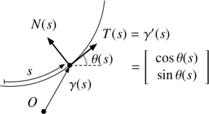
Figure 1: Smooth planar curve and the Frenet frame.

The Euler’s elastica (or simply referred to as the elastica) is defined as a critical point of the elastic energy

$$E=\int_{0}^{L}\big{(}\kappa(s)\big{)}^{2}\,ds,$$ (2.5)

with respect to variations with fixed endpoints and tangent vectors at the endpoints, under the condition of preserving the total length. The Euler-Lagrange equation yields the following differential equations for the curvature and the angle function:

Proposition 2.1.

The curvature $\kappa$ of the Euler’s elastica satisfies

$$\kappa^{\prime\prime}+\frac{1}{2}\kappa^{3}-\lambda\kappa=0,$$ (2.6)

where $\lambda\in\mathbb{R}$ is a constant. Moreover, the angle function $\theta$ satisfies

$$\theta^{\prime\prime}+\mu\sin\theta=0,$$ (2.7)

where $\mu>0$ is a constant.

Derivation of equation (2.6) is given in various literatures such as [29]. Here, we show a concise derivation using the variation of the tangent vector. Consider the functional

$$S=\int_{0}^{L}\Big{(}\langle T^{\prime},T^{\prime}\rangle+c\langle T,T\rangle+\langle a,T\rangle\Big{)}\,ds,$$ (2.8)

where the first term is the elastic energy, and the second and third terms correspond to the preservation $\left\lVert T\right\rVert$ and $\gamma(L)-\gamma(0)$, respectively, with $c=c(s)\in\mathbb{R}$ and $a\in\mathbb{R}^{2}$ being the Lagrange multipliers. The variation of $S$ is calculated by using the Frenet formula (2.4) as

$$\delta S =\int_{0}^{L}\Big{(}2\langle T^{\prime},\delta T^{\prime}\rangle+2c(s)\langle T,\delta T\rangle+\langle a,\delta T\rangle\Big{)}\,ds$$

$$=2\langle T^{\prime},\delta T\rangle\Big{|}_{0}^{L}+2\int_{0}^{L}\big{\langle}(\kappa^{2}+c(s))T-\kappa^{\prime}N+\frac{a}{2},\delta T\big{\rangle}\,ds.$$ (2.9)

The first term is the boundary term that vanishes due to the boundary condition, and the second term gives the Euler-Lagrange equation,

$$(\kappa^{2}+c)\,T-\kappa^{\prime}N+\frac{a}{2}=0.$$ (2.10)

Taking the scalar product with $T$ and $N$, we have

$$\kappa^{2}+c+\frac{1}{2}\langle a,T\rangle=0\quad\text{and}\quad-\kappa^{\prime}+\frac{1}{2}\langle a,N\rangle=0,$$ (2.11)

respectively. Multiplying $\kappa^{\prime}$ to both sides of the second equation of equation (2.11), we find that it is integrated to give

$$\frac{\kappa^{2}}{2}-\lambda=\frac{1}{2}\langle a,T\rangle,$$ (2.12)

where $\lambda\in\mathbb{R}$ is a constant of integration. Eliminating $\langle a,T\rangle$ from the first equation of (2.11) and equation (2.12), $c$ is determined consistently as $c=-\frac{3}{2}\kappa^{2}+\lambda$. Differentiating the second equation of equation (2.11) gives

$$\kappa^{\prime\prime}=-\frac{\kappa}{2}\langle a,T\rangle.$$ (2.13)

Then eliminating $\langle a,T\rangle$ from equations (2.12) and (2.13) yields

$$\kappa^{\prime\prime}+\kappa\Big{(}\frac{\kappa^{2}}{2}-\lambda\Big{)}=0,$$ (2.14)

which is nothing but equation (2.6).

Remark 2.2.

1. Equation (2.6) is derived from equation (2.7) as follows. Multiplying $\theta^{\prime}$ on both sides of equation (2.7), we see that equation (2.7) is integrated to give

   $$\frac{1}{2}(\theta^{\prime})^{2}=\mu\cos\theta+\lambda,$$ (2.15)

   where $\lambda$ is a constant of integration. Then differentiating equation (2.7) and using equation (2.15) yields

   $$\kappa^{\prime\prime}=-\mu\cos\theta\times\theta^{\prime}=\Big{(}-\frac{1}{2}\kappa^{2}+\lambda\Big{)}\kappa,$$ (2.16)

   which is nothing but equation (2.6).

2. Equations (2.6) and (2.7) can be seen as travelling-wave reductions of the (focusing) modified KdV equation

   $$\frac{\partial\kappa}{\partial t}+\frac{3}{2}\kappa^{2}\frac{\partial\kappa}{\partial s}+\frac{\partial^{3}\kappa}{\partial s^{3}}=0$$ (2.17)

   and the sine-Gordon equation,

   $$\frac{\partial^{2}\theta}{\partial s\partial y}=\sin\theta,$$ (2.18)

   respectively, where the former describes the integrable deformation of planar curves [8, 13].

It is known that the differential equations (2.6) and (2.7) can be solved in terms of the Jacobi elliptic functions. This is well-known, but we present the solutions for the readers’ convenience. In the literature, the solutions are often constructed from the the first integral of (2.6) given by

$$(\kappa^{\prime})^{2}+\frac{\kappa^{4}}{2}-\lambda\kappa^{2}=C,$$ (2.19)

where $C$ is a conserved quantity (constant). Here we present those solutions and verify them by the differential equations for the Jacobi elliptic functions.

Proposition 2.3.

The curvature $\kappa$ and the angle function $\theta$ can be expressed in terms of the Jacobi elliptic functions as follows:
(i)

$$\kappa=2k^{-1}\sqrt{\mu}\,\operatorname{dn}\,\Big{(}k^{-1}\sqrt{\mu}s;k\Big{)},$$ (2.20)

$$\sin\frac{\theta}{2}=\operatorname{sn}\Big{(}k^{-1}\sqrt{\mu}s;k\Big{)},\quad\mu=\frac{\lambda}{2k^{-2}-1}.$$ (2.21)

(ii)

$$\kappa=2k\sqrt{\mu}\,\operatorname{cn}\,\Big{(}\sqrt{\mu}s;k\Big{)},$$ (2.22)

$$\sin\frac{\theta}{2}=k\operatorname{sn}\Big{(}\sqrt{\mu}s;k\Big{)},\quad\mu=\frac{\lambda}{2k^{2}-1}.$$ (2.23)

Proof.

It can be easily verified that equations (2.20) and (2.22) satisfy equation (2.6) from the differential equations for the $\operatorname{dn}$ and $\operatorname{cn}$ functions [24]

$$y=\operatorname{dn}(x,k),\quad\frac{d^{2}y}{dx^{2}}=(2-k^{2})y-2y^{3},$$ (2.24)

$$y=\operatorname{cn}(x,k),\quad\frac{d^{2}y}{dx^{2}}=(2k^{2}-1)y-2k^{2}y^{3},$$ (2.25)

respectively, by applying suitable scale transformations. Also, equations (2.21) and (2.23) are shown to satisfy equation (2.7) in a similar manner. ∎

Remark 2.4.

The Jacobi elliptic functions can be extended to modules $k>1$, see, for example, [17, 24]. Thus, there exists an analytic continuation for all Jacobi elliptic functions in the range $k\geq 0$. In this way, cases (i) and (ii) can be regarded as one. As it is known, the case (i) (resp. (ii)) yields the elastica without (resp. with) inflection points; see Figure 4.

3 Integrable discrete Euler’s elastica

3.1 Basic framework of discrete planar curves

We first introduce the basic framework for discrete planar curves [12, 14, 20]. Let $\gamma_{n}\in\mathbb{R}^{2}$ ($n\in\mathbb{Z}$) be a discrete planar curve with $|\gamma_{n+1}-\gamma_{n}|=h$, where $h>0$ is a constant. We also assume $\det{\big{(}\gamma_{n+1}-\gamma_{n},\gamma_{n}-\gamma_{n-1}\big{)}}\neq 0$, i.e., not three consecutive points are collinear. Then $\gamma_{n}$ is called a discrete planar curve with segment length $h$. We define the discrete tangent and normal vectors by

$$T_{n}=\frac{\gamma_{n+1}-\gamma_{n}}{h}=\left[\begin{array}[]{c}\cos\Theta_{n}\\ \sin\Theta_{n}\end{array}\right]\quad\text{and}\quad N_{n}=R\Big{(}\frac{\pi}{2}\Big{)}T_{n},$$ (3.1)

respectively, where the discrete angle function $\Theta_{n}$ is the angle of $T_{n}$ measured from the horizontal axis in the counterclockwise direction. The discrete Frenet frame is defined by

$$\Phi_{n}=[T_{n},N_{n}]\in{\rm SO}(2),$$ (3.2)

and the discrete Frenet formula by

$$\Phi_{n+1}=\Phi_{n}L_{n},\quad L_{n}=R(K_{n+1}),$$ (3.3)

where $K_{n}=\Theta_{n}-\Theta_{n-1}$ is the angle between two adjacent tangent vectors. Equation (3.3) is the discrete version of the Frenet formula (2.4); see Figure 3. The discrete curvature $\kappa_{n}$ can be defined as the reciprocal of the radius $\rho_{n}$ of the osculating circle touching two adjacent segments at their midpoints [12] (see Figure 3),

$$\kappa_{n}=\frac{1}{\rho_{n}}=\frac{2}{h}\tan\frac{K_{n}}{2}.$$ (3.4)

We note that the discrete Frenet formula (3.3) can be written in terms of $\kappa_{n}$ as

$$\frac{\Phi_{n}-\Phi_{n-1}}{h}=\frac{\Phi_{n}+\Phi_{n-1}}{2}\left[\begin{array}[]{cc}0&-\kappa_{n}\\ \kappa_{n}&0\end{array}\right].$$ (3.5)

Figure 2: Discrete planar curve and the Frenet frame.

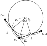
Figure 3: Discrete curvature of discrete arc length planar curve.

3.2 Discrete Euler’s elastica

The discrete Euler’s elastica [3, 4, 11] is defined as a discrete planar curve $\gamma_{n}$ with segment length $h$ that is a critical point of the functional

$$E_{d}=\sum_{n=1}^{N-1}\frac{2}{h}\log\left(1+\frac{h^{2}}{4}\kappa_{n}^{2}\right)\cong\sum_{n=1}^{N-1}\frac{2}{h}\log\big{(}1+\langle T_{n-1},T_{n}\rangle),$$ (3.6)

with respect to variation with fixed endpoints and end edges. Note that $\cong$ means that the two functionals yield the same critical points. As mentioned in [4], $E_{d}$ can be regarded as a discrete analogue of the elastic energy (2.5), in a sense that $2/h\log(1+h^{2}\kappa_{n}^{2}/4)$ is the potential energy of the bending force proportional to the discrete curvature $\kappa_{n}$ at each vertex.

Taking into account the preservation of $\left\lVert\gamma_{n}-\gamma_{n-1}\right\rVert$ and $\gamma_{N}-\gamma_{0}$ by introducing the Lagrange multipliers $c_{n}\in\mathbb{R}$ and $a\in\mathbb{R}^{2}$, respectively, consider the functional

$$S_{d}=\sum_{n=1}^{N-1}\frac{2}{h}\log\big{(}1+\langle T_{n-1},T_{n}\rangle)+\sum_{n=0}^{N-1}\big{(}c_{n}\langle T_{n},T_{n}\rangle+h\langle a,T_{n}\rangle\big{)}.$$ (3.7)

Proposition 3.1.

The Euler-Lagrange equation for the functional (3.7) is given by

$$\frac{2}{h}\frac{T_{n-1}}{1+\langle T_{n-1},T_{n}\rangle}+\frac{2}{h}\frac{T_{n+1}}{1+\langle T_{n},T_{n+1}\rangle}+2c_{n}T_{n}+ha=0,$$ (3.8)

or, equivalently, in terms of the discrete curvature $\kappa_{n}$ by

$$\kappa_{n+1}+\kappa_{n-1}=\frac{\alpha\kappa_{n}}{1+\frac{h^{2}}{4}\kappa_{n}^{2}},$$ (3.9)

where $\alpha\in\mathbb{R}$ is a constant.

Proof.

The variation of $S_{d}$ is calculated as follows:

$$\delta S_{d} =\sum_{n=1}^{N-1}\Big{(}\frac{2}{h}\frac{\langle\delta T_{n-1},T_{n}\rangle}{1+\langle T_{n-1},T_{n}\rangle}+\frac{2}{h}\frac{\langle T_{n-1},\delta T_{n}\rangle}{1+\langle T_{n-1},T_{n}\rangle}\Big{)}+\sum_{n=0}^{N-1}\Big{(}2c_{n}\langle T_{n},\delta T_{n}\rangle+h\langle a,\delta T_{n}\rangle\Big{)}$$

$$=R+\sum_{n=1}^{N-2}\Big{\langle}\frac{2}{h}\frac{T_{n-1}}{1+\langle T_{n-1},T_{n}\rangle}+\frac{2}{h}\frac{T_{n+1}}{1+\langle T_{n},T_{n+1}\rangle}+2c_{n}T_{n}+ha,\delta T_{n}\Big{\rangle},$$ (3.10)

where $R$ is the boundary term given by

$$R=\Big{\langle}\frac{2}{h}\frac{T_{1}}{1+\langle T_{0},T_{1}\rangle}+2c_{0}T_{0}+ha,\delta T_{0}\Big{\rangle}+\Big{\langle}\frac{2}{h}\frac{T_{N-2}}{1+\langle T_{N-2},T_{N-1}\rangle}+2c_{N-1}T_{N-1}+ha,\delta T_{N-1}\Big{\rangle},$$

which vanishes due to the boundary condition. Setting $\delta S_{d}=0$ gives the Euler-Lagrange equation,

$$\frac{2}{h}\frac{T_{n-1}}{1+\langle T_{n-1},T_{n}\rangle}+\frac{2}{h}\frac{T_{n+1}}{1+\langle T_{n},T_{n+1}\rangle}+2c_{n}T_{n}+ha=0,$$ (3.11)

which proves the first part. For the second part we use the discrete Frenet formula (3.5) written explicitly in terms of the tangent and normal vectors,

$$\frac{T_{n}-T_{n-1}}{h}=\kappa_{n}\frac{N_{n}+N_{n-1}}{2},\qquad\frac{N_{n}-N_{n-1}}{h}=-\kappa_{n}\frac{T_{n}+T_{n-1}}{2}.$$ (3.12)

From the discrete Frenet formula (3.3) and equation (3.4) we have that

$$\frac{2}{h}\frac{\langle T_{n-1},N_{n}\rangle}{1+\langle T_{n-1},T_{n}\rangle}=-\kappa_{n},\quad\frac{2}{h}\frac{\langle T_{n},N_{n}\rangle}{1+\langle T_{n},T_{n+1}\rangle}=\kappa_{n+1},$$ (3.13)

thus taking the inner product of both hand sides of equation (3.8) with $N_{n}$ gives

$$\kappa_{n}-\kappa_{n+1}=h\langle a,N_{n}\rangle.$$ (3.14)

Then, taking the inner product of the first equation in the discrete Frenet formula (3.12) with $a$ gives

$$\left<{a},{T_{n}}\right>-\left<{a},{T_{n-1}}\right>=-\frac{1}{2}\kappa_{n}\kappa_{n+1}+\frac{1}{2}\kappa_{n-1}\kappa_{n},$$ (3.15)

which implies that exists a constant $\lambda\in\mathbb{R}$ such that

$$\left<{a},{T_{n}}\right>=-\frac{1}{2}\kappa_{n}\kappa_{n+1}+\lambda.$$ (3.16)

Finally taking the inner product of the second equation in the discrete Frenet formula (3.12) with $a$, and using equations (3.14) and (3.16), yields

$$(\kappa_{n+1}+\kappa_{n-1})\left(1+\frac{h^{2}}{4}\kappa_{n}^{2}\right)=(2+h^{2}\lambda)\kappa_{n},$$ (3.17)

which is exactly equation (3.9) with $\alpha=2+h^{2}\lambda$. ∎

By using a technique similar to the one shown in [31], we construct explicit solutions to equation (3.9) from its discrete first integral,

$$\kappa_{n+1}^{2}+\kappa_{n}^{2}-\alpha\kappa_{n+1}\kappa_{n}+\frac{h^{2}}{4}\kappa_{n+1}^{2}\kappa_{n}^{2}=C,$$ (3.18)

where $C\in\mathbb{R}$ is a constant (conserved quantity). Here, we avoid the long computation required and simply present the solutions corresponding to equations (2.20) and (2.22), and verify them by using the addition formulas for the Jacobi elliptic functions.

Proposition 3.2.

Let $z\in\mathbb{R}$ be a constant. Then the following functions satisfy equation (3.9).
(i)

$$\begin{split}&\kappa_{n}=\frac{2}{h}\frac{\operatorname{sn}(k^{-1}z;k)}{\operatorname{cn}(k^{-1}z;k)}\,\operatorname{dn}\,(k^{-1}zn;k),\\[5.69054pt] &\alpha=2\frac{\operatorname{dn}(k^{-1}z;k)}{\operatorname{cn}^{2}(k^{-1}z;k)}.\end{split}$$ (3.19)

(ii)

$$\begin{split}&\kappa_{n}=\frac{2}{h}\frac{k\operatorname{sn}(z;k)}{\operatorname{dn}(z;k)}\,\operatorname{cn}(zn;k),\\[5.69054pt] &\alpha=2\frac{\operatorname{cn}(z;k)}{\operatorname{dn}^{2}(z;k)}.\end{split}$$ (3.20)

Proof.

These solutions are verified directly by the addition formulas for the $\operatorname{dn}$ and $\operatorname{cn}$ functions [24]. On the one hand, we use that

$$\operatorname{dn}(u+v)+\operatorname{dn}(u-v)=\frac{\frac{2\operatorname{dn}v}{\operatorname{cn}^{2}v}\operatorname{dn}u}{1+\frac{\operatorname{sn}^{2}v}{\operatorname{cn}^{2}v}\operatorname{dn}^{2}u}.$$ (3.21)

Putting $u=k^{-1}zn$, $v=k^{-1}z$ and $\kappa_{n}=a\operatorname{dn}(u;k)$, and comparing equation (3.21) with equation (3.9), we see that

$$\frac{1}{a^{2}}\frac{\operatorname{sn}^{2}v}{\operatorname{cn}^{2}v}=\frac{h^{2}}{4},\qquad\frac{2\operatorname{dn}v}{\operatorname{cn}^{2}v}=\alpha,$$ (3.22)

which proves (i). Similarly, on the other hand we use

$$\operatorname{cn}(u+v)+\operatorname{cn}(u-v)=\frac{\frac{2\operatorname{cn}v}{\operatorname{dn}^{2}v}\operatorname{cn}u}{1+\frac{k^{2}\operatorname{sn}^{2}v}{\operatorname{dn}^{2}v}\operatorname{cn}^{2}u}.$$ (3.23)

Then putting $u=zn$, $v=z$ and $\kappa_{n}=b\operatorname{cn}(u;k)$, we get equation (3.9) with

$$\frac{1}{b^{2}}\frac{k^{2}\operatorname{sn}^{2}v}{\operatorname{dn}^{2}v}=\frac{h^{2}}{4},\qquad\frac{2\operatorname{cn}v}{\operatorname{dn}^{2}v}=\alpha,$$ (3.24)

which proves (ii). ∎

Remark 3.3.

1. Comparing equations (2.20) and (3.19), we see that there exists a constant $\Omega$ such that $\kappa_{n}=\kappa(\Omega n)$. Indeed, we have

   $$\Omega=\frac{v}{\sqrt{\frac{\lambda}{2-k^{2}}}}\quad\text{and}\quad v=\operatorname{sn}^{-1}\sqrt{\frac{\frac{\lambda h^{2}}{2-k^{2}}}{1+\frac{\lambda h^{2}}{2-k^{2}}}}.$$ (3.25)

   There is also a similar relationship between equations (2.22) and (3.20). This implies that the discrete curvature $\kappa_{n}$ is an “exact discretization” of the smooth curvature $\kappa(s)$.

2. By putting $\alpha=h^{2}\lambda+2$ and $nh=s$, equation (3.9) yields equation (2.6) in the continuum limit $h\to 0$. On the level of solutions, the following parametrizations of $z$,

   $$z= \sqrt{\frac{\lambda}{2k^{-2}-1}}\,h$$ for (i), (3.26)

   $$z= \sqrt{\frac{\lambda}{2k^{2}-1}}\,h$$ for (ii), (3.27)

   are consistent in the continuum limit to equations (2.21) and (2.23), respectively.

3. Equation (3.9) is also known as the McMillan map, which is a special case of the Quispel-Roberts-Thompson (QRT) map solved by elliptic functions [26]. It can also be regarded as an autonomous version of a discrete Painlevé II equation [15, 16, 27]

4. It is known that position vectors of both smooth and discrete elasticae admit explicit formulas in terms of the elliptic theta functions [21, 23].

Figure 4 illustrates typical examples of both smooth and discrete elasticae.

Figure 4: Typical examples of smooth and discrete elasticae. Left: (ii) $k=0.8$, middle: (i) $k=0.909$, right: (ii) $k=0.9089\ldots$ (smooth), $k=0.919\ldots$ (discrete).

3.3 Discrete Euler’s elastica in terms of a potential function

Following [13], we say that $\theta_{n}$ is a potential function if it is such that

$$\Theta_{n}=\frac{\theta_{n+1}+\theta_{n}}{2}.$$ (3.28)

In this context, the discrete curvature is written as

$$\kappa_{n}=\frac{2}{h}\tan\left(\frac{\theta_{n+1}-\theta_{n-1}}{4}\right).$$ (3.29)

Proposition 3.4.

Suppose that $\theta_{n}$ satisfies

$$\sin\left(\frac{\theta_{n+1}-2\theta_{n}+\theta_{n-1}}{4}\right)+\epsilon\sin\left(\frac{\theta_{n+1}+2\theta_{n}+\theta_{n-1}}{4}\right)=0,$$ (3.30)

where $\epsilon\in\mathbb{R}$ is a constant. Then we have:

1. It holds that

   $$\cos\left(\frac{\theta_{n+1}-\theta_{n}}{2}\right)+\epsilon\cos\left(\frac{\theta_{n+1}+\theta_{n}}{2}\right)=\Lambda,$$ (3.31)

   where $\Lambda\in\mathbb{R}$ is a constant.

2. The discrete curvature satisfies equation (3.9) with $\alpha=2(1-\epsilon^{2})/\Lambda^{2}$.

Proof.

The first statement is shown as follows. Multiplying $\sin(\frac{\theta_{n+1}-\theta_{n-1}}{4})$ to equation (3.30), using the product-to-sum formula, and rearranging terms gives:

$$\cos\left(\frac{\theta_{n+1}-\theta_{n}}{2}\right)+\epsilon\cos\left(\frac{\theta_{n+1}+\theta_{n}}{2}\right)=\cos\left(\frac{\theta_{n}-\theta_{n-1}}{2}\right)+\epsilon\cos\left(\frac{\theta_{n}+\theta_{n-1}}{2}\right),$$ (3.32)

which implies (3.31). In order to show the second statement, we introduce

$$\varphi_{n}=\frac{\theta_{n+1}-\theta_{n}}{2},\qquad\psi_{n}=\frac{\theta_{n+1}+\theta_{n}}{2},$$ (3.33)

for simplicity in the notation. We have that $K_{n}=\psi_{n}-\psi_{n-1}=\varphi_{n}+\varphi_{n-1}$, and equation (3.30) is rewritten as

$$\sin\left(\frac{\varphi_{n}-\varphi_{n-1}}{2}\right)=-\epsilon\sin\left(\frac{\psi_{n}+\psi_{n-1}}{2}\right).$$ (3.34)

We expand equation (3.34) as

$$\sin\varphi_{n}\cos\frac{K_{n}}{2}-\cos\varphi_{n}\sin\frac{K_{n}}{2}=-\epsilon\sin\psi_{n}\cos\frac{K_{n}}{2}+\epsilon\cos\psi_{n}\sin\frac{K_{n}}{2},$$ (3.35)

which gives

$$\tan\frac{K_{n}}{2}=\frac{\sin\varphi_{n}+\epsilon\sin\psi_{n}}{\Lambda}\quad\text{and}\quad\tan\frac{K_{n+1}}{2}=\frac{\sin\varphi_{n}-\epsilon\sin\psi_{n}}{\Lambda},$$ (3.36)

where we used equation (3.31). From equation (3.36) and the sum-to-product formula, we have

$$\Lambda\Big{(}\tan\frac{K_{n+1}}{2}+\tan\frac{K_{n-1}}{2}\Big{)}=2\sin\frac{K_{n}}{2}\Big{[}\cos\Big{(}\frac{\varphi_{n}-\varphi_{n-1}}{2}\Big{)}-\epsilon\cos\Big{(}\frac{\psi_{n}+\psi_{n-1}}{2}\Big{)}\Big{]}.$$ (3.37)

We use the following two expressions: On the one hand, from equation (3.30),

$$\cos^{2}\Big{(}\frac{\varphi_{n}-\varphi_{n-1}}{2}\Big{)}-\epsilon^{2}\cos^{2}\Big{(}\frac{\psi_{n}+\psi_{n-1}}{2}\Big{)}=1-\epsilon^{2}.$$ (3.38)

On the other hand,

$$\cos\Big{(}\frac{\varphi_{n}-\varphi_{n-1}}{2}\Big{)}+\epsilon\cos\Big{(}\frac{\psi_{n}+\psi_{n-1}}{2}\Big{)} =\cos\frac{K_{n}}{2}\left(\cos\varphi_{n}+\epsilon\cos\psi_{n}\right)+\sin\frac{K_{n}}{2}\left(\sin\varphi_{n}+\epsilon\sin\psi_{n}\right)$$

$$=\frac{\Lambda}{\cos\frac{K_{n}}{2}},$$ (3.39)

where we used equation (3.31) and (3.36). Finally, we multiply equation (3.37) by equation (3.3) to obtain

$$\Lambda\Big{(}\tan\frac{K_{n+1}}{2}+\tan\frac{K_{n-1}}{2}\Big{)}{prop:sogo}\frac{\Lambda}{\cos\frac{K_{n}}{2}}=2\sin\frac{K_{n}}{2}(1-\epsilon^{2}),$$ (3.40)

where we used (3.38), which is rewritten as

$$\tan\frac{K_{n+1}}{2}+\tan\frac{K_{n-1}}{2}=\frac{1-\epsilon^{2}}{\Lambda^{2}}\frac{2\tan\frac{K_{n}}{2}}{1+\tan^{2}\frac{K_{n}}{2}}.$$ (3.41)

From the definition of discrete curvature, equation (3.41) is equivalent to equation (3.9) with $\alpha=2(1-\epsilon^{2})/\Lambda^{2}$, which proves the second statement. ∎

Remark 3.5.

Proposition 3.4 provides discrete analogues for equations (2.7) and (2.15). In fact, by putting

$$\Lambda=1-\frac{h^{2}}{4}\lambda,\quad\epsilon=\frac{h^{2}}{4}\mu,\quad s=nh,$$ (3.42)

equations (3.30) and (3.31) yield equations (2.7) and (2.15) in the continuum limit $h\to 0$.

We next present explicit solutions for equation (3.30). Part of Proposition 3.6 and 3.8 can be found in [30], in a slightly different context: in that work, the function $\theta_{n}$ is regarded as the angle function (here denoted as $\Theta_{n}$) instead of a potential function.

Proposition 3.6.

The following functions satisfy equation (3.30):
(i)

$$\sin\frac{\theta_{n}}{2}=\operatorname{sn}(k^{-1}zn;k),\quad\operatorname{dn}(k^{-1}z;k)=\frac{1-\epsilon}{1+\epsilon}.$$ (3.43)

(ii)

$$\sin\frac{\theta_{n}}{2}=k\operatorname{sn}(zn;k),\quad\operatorname{cn}(z;k)=\frac{1-\epsilon}{1+\epsilon}.$$ (3.44)

Proof.

For convenience, we write $u=k^{-1}zn$ and $v=k^{-1}z$. For (i), we show that equation (3.43) satisfies equation (3.31). Note that $\cos(\theta_{n}/2)=\operatorname{cn}u$ and $\cos(\theta_{n+1}/2)=\operatorname{cn}(u+v)$. Then, the right hand side of equation (3.31) is rewritten as

$$\cos\left(\frac{\theta_{n+1}-\theta_{n}}{2}\right)+\epsilon\cos\left(\frac{\theta_{n+1}+\theta_{n}}{2}\right)=\frac{1}{1-k^{2}\operatorname{sn}^{2}u\operatorname{sn}^{2}v}\\ \times\Big{[}\big{\{}(1+\epsilon)\operatorname{cn}^{2}u+(1-\epsilon)\operatorname{sn}^{2}u\operatorname{dn}v\big{\}}\operatorname{cn}v+\big{\{}-(1+\epsilon)\operatorname{dn}v+(1+\epsilon)\big{\}}\operatorname{sn}u\operatorname{sn}v\operatorname{cn}u\operatorname{dn}v\Big{]},$$ (3.45)

where we used the addition formulas for the $\operatorname{cn}$ and $\operatorname{sn}$ functions. Imposing $\operatorname{dn}v=(1+\epsilon)/(1-\epsilon)$, we see that equation (3.31) is consistently reduced to $\Lambda=(1+\epsilon)\operatorname{cn}v$. We prove (ii) in a similar manner. In fact, noticing that $\cos(\theta_{n}/2)=\operatorname{dn}u$ and imposing $\operatorname{cn}v=(1+\epsilon)(1-\epsilon)$, equation (3.31), with $u=zn$ and $v=z$, is consistently reduced to $\Lambda=(1+\epsilon)\operatorname{dn}v$. ∎

Remark 3.7.

1. In case (i), the parameter $\alpha$ in equation (3.9) is given by

   $$\alpha=2\frac{(1-\epsilon^{2})}{\Lambda^{2}}=2\frac{\operatorname{dn}(k^{-1}z;k)}{\operatorname{cn}^{2}(k^{-1}z;k)},$$ (3.46)

   which implies that $\theta_{n}$ in equation (3.43) corresponds to $\kappa_{n}$ in equation (3.19). In case (ii),

   $$\alpha=2\frac{(1-\epsilon^{2})}{\Lambda^{2}}=2\frac{\operatorname{cn}(z;k)}{\operatorname{dn}^{2}(z;k)},$$ (3.47)

   so that $\theta_{n}$ in equation (3.44) corresponds to $\kappa_{n}$ in equation (3.20). These correspondences can be verified directly by computing $\kappa_{n}$ from equations (3.43) and (3.44), respectively.

2. Continuum limits of equations (3.43) and (3.44) to equations (3.19) and (3.20), respectively, are obtained by putting $\epsilon=\frac{\mu}{4}h^{2}$ and taking the limit of $h\to 0$. This is consistent with Remark 3.3.

We finally present the variational formulation for equation (3.30).

Proposition 3.8 ([30], Sec. 2).

Equation (3.30) is equivalent to the Euler-Lagrange equation of the functional

$$\tilde{S}_{d}=\sum_{n=0}^{N-1}\cos\left(\frac{\theta_{n+1}-\theta_{n}}{2}\right)-\epsilon\cos\left(\frac{\theta_{n+1}+\theta_{n}}{2}\right),$$ (3.48)

with respect to variations of the potential angle $\theta_{n}$ with fixed endpoints.

Proof.

Let $L(\theta_{n},\theta_{n+1})=\cos\left((\theta_{n+1}-\theta_{n})/2\right)-\epsilon\cos\left((\theta_{n+1}+\theta_{n})/2\right)$. Then, the Euler-Lagrange equation is calculated as

$$0 =\frac{\partial}{\partial\theta_{n}}L(\theta_{n},\theta_{n+1})+\frac{\partial}{\partial\theta_{n}}L(\theta_{n-1},\theta_{n})$$

$$=\cos\left(\frac{\theta_{n+1}-\theta_{n-1}}{4}\right)\left[\sin\left(\frac{\theta_{n+1}-2\theta_{n}+\theta_{n-1}}{4}\right)+\epsilon\sin\left(\frac{\theta_{n+1}+2\theta_{n}+\theta_{n-1}}{4}\right)\right],$$ (3.49)

which gives equation (3.30). ∎

Remark 3.9.

Equation (3.30) can be seen as a reduction of two well known equations:

1. The discrete sine-Gordon equation [2, 10, 14],

   $$\sin\left(\frac{\theta_{l+1}^{m+1}-\theta_{l}^{m+1}-\theta_{l+1}^{m}+\theta_{l}^{m}}{4}\right)=\frac{a}{b}\sin\left(\frac{\theta_{l+1}^{m+1}+\theta_{l}^{m+1}+\theta_{l+1}^{m}+\theta_{l}^{m}}{4}\right),$$ (3.50)

   where $a$, $b$ are lattice intervals. In fact, assuming that $\theta$ depends only on $n=l+m$, equation (3.50) is reduced to equation (3.30) with $\epsilon=-\frac{b}{a}$.

2. The discrete potential modified KdV equation [9],

   $$\tan\frac{\theta_{l+1}^{m+1}-\theta_{l}^{m}}{4}=\frac{b+a}{b-a}\tan\frac{\theta_{l}^{m+1}-\theta_{l+1}^{m}}{4},$$ (3.51)

   or equivalently

   $$\sin\left(\frac{\theta_{l+1}^{m+1}-\theta_{l}^{m+1}+\theta_{l+1}^{m}-\theta_{l}^{m}}{4}\right)=\frac{a}{b}\sin\left(\frac{\theta_{l+1}^{m+1}+\theta_{l}^{m+1}-\theta_{l+1}^{m}-\theta_{l}^{m}}{4}\right),$$ (3.52)

   which describes the isoperimetric and equidistant deformation of discrete planar curves [13, 20], is transformed to the discrete sine-Gordon equation (3.50) by $\theta_{l}^{m}\to(-1)^{m}\theta_{l}^{m}$. In this sense, equation (3.30) can also be regarded as a reduction of the discrete potential modified KdV equation.

4 Approximation of discrete curves

In this section, we construct an algorithm to approximate a given discrete planar curve to a discrete elastica. Among the many possible discretizations for the elastica, the advantages of using the one shown in this work can be described as follows: First, the discrete elasticae are endowed with the same integrable structure as in their smooth counterpart, i.e., they possess several conserved quantities, can be obtained via a variational principle, and their explicit solutions are expressed in terms of Jacobi elliptic functions. Moreover, it is known that variational integrators have controlled error in their solutions [7, 18, 25]. In particular, the explicit expression for the discrete curvature $\kappa_{n}$ is an “exact discretization” of the smooth curvature $\kappa(s)$ as discussed in Remark 3.3, and the potential function $\theta_{n}$ has the same functional shape as the smooth angle function $\theta(s)$. From these observations, we expect this discretization to have good numerical properties.

4.1 General discrete Euler’s elastica segment

To describe a general curve segment in the plane, we include the freedom of rotation in the equations. We do this by shifting the angle function and discrete angle function by a constant $\phi\in\mathbb{R}$ in all the expressions. In particular, equation (3.30) goes to

$$\sin\left(\frac{\theta_{n+1}-2\theta_{n}+\theta_{n-1}}{4}\right)+\frac{\mu h^{2}}{4}\sin\left(\frac{\theta_{n+1}+2\theta_{n}+\theta_{n-1}}{4}-\phi\right)=0,$$ (4.1)

where we put $\epsilon=\mu h^{2}/4$, with $\mu>0$ a constant. From Proposition 3.6, we have
(i)

$$\cos\frac{\theta_{n}-\phi}{2}=\operatorname{cn}(k^{-1}(zn+q);k),\quad\sin\frac{\theta_{n}-\phi}{2}=\operatorname{sn}(k^{-1}(zn+q);k),$$ (4.2)

(ii)

$$\cos\frac{\theta_{n}-\phi}{2}=\operatorname{dn}(zn+q;k),\quad\sin\frac{\theta_{n}-\phi}{2}=k\operatorname{sn}(zn+q;k),$$ (4.3)

where $k>0$, $q,z\in\mathbb{R}$ are constants. The parameter $k$ determines the shape of the elastica, $q$ the initial point, and $z$ is related with the length and point aggregation of the curve segment. Finally, from its starting point $\gamma_{0}\in\mathbb{R}^{2}$, a discrete elastica segment is calculated recursively by

$$\gamma_{n}=\gamma_{n-1}+h\left[\begin{array}[]{c}\cos\left(\frac{\theta_{n+1}-\phi}{2}+\frac{\theta_{n}-\phi}{2}-\phi\right)\\ \sin\left(\frac{\theta_{n+1}-\phi}{2}+\frac{\theta_{n}-\phi}{2}-\phi\right)\end{array}\right]\qquad\text{for all }n=1,\dots,N-1.$$ (4.4)

Note that we can expand the sine and cosine in equation (4.4) and make use of equation (4.3) to obtain an explicit expression in terms of the Jacobi elliptic functions. We conclude that a general discrete elastica segment can be characterized by seven parameters:

$$p=(x_{0},y_{0},h,\phi,z,q,k),$$ (4.5)

where $x_{0},y_{0}\in\mathbb{R}$ are the two components of the initial point $\gamma_{0}$. We write as $\gamma_{n}(p)$ to the discrete elastica with parameters $p$.

4.2 Fairing process

Given a general discrete curve segment $\zeta_{n}\in\mathbb{R}^{2}$ ($n=0,\dots,N-1$), we look for a discrete elastica $\gamma_{n}(p)\in\mathbb{R}^{2}$ that is the closest, in a $L^{2}$-distance sense, to $\zeta_{n}$. Namely, we seek to find $p^{*}$ such that

$$p^{*}=\operatorname*{arg\,min}_{p\in U}\left\{\sum_{n=0}^{N-1}\frac{1}{2}\left\lVert\gamma_{n}(p)-\zeta_{n}\right\rVert^{2}\right\},$$ (4.6)

where

$$U=\left\{(x_{0},y_{0},h,\phi,z,q,k)\operatorname{|}x_{0},y_{0},\phi,z,q\in\mathbb{R}\wedge h,k>0\right\}.$$ (4.7)

We solve this non-convex problem using the Interior Point Optimizer (IPOPT) package, that for our purpose can be seen as a gradient descent-like method for nonlinear optimizations [32]. For its implementation we need to compute the gradient and the Hessian of the objective function

$$\mathcal{L}(p):=\sum_{n=0}^{N-1}\frac{1}{2}\left\lVert\gamma_{n}(p)-\zeta_{n}\right\rVert^{2}.$$ (4.8)

For the gradient, we have

$$\frac{\partial}{\partial p_{i}}\mathcal{L}(p)=\sum_{n=0}^{N-1}\left<{\gamma_{n}(p)-\zeta_{n}},{\frac{\partial}{\partial p_{i}}\gamma_{n}(p)}\right>,\qquad p_{i}=x_{0},y_{0},h,\phi,z,q,k,$$ (4.9)

which is computed recursively from equation (4.4),

$$\frac{\partial}{\partial p_{i}}\gamma_{n}(p)=\frac{\partial}{\partial p_{i}}\gamma_{n-1}(p)+\begin{cases}0&p_{i}=x_{0},y_{0},\\ T_{n}&p_{i}=h,\\ h\frac{\partial}{\partial p_{i}}T_{n}&\text{otherwise},\end{cases}\qquad\frac{\partial}{\partial p_{i}}\gamma_{0}=\begin{cases}\left(\begin{smallmatrix}1\\ 0\end{smallmatrix}\right)&p_{i}=x_{0},\\ \left(\begin{smallmatrix}0\\ 1\end{smallmatrix}\right)&p_{i}=y_{0},\\ \left(\begin{smallmatrix}0\\ 0\end{smallmatrix}\right)&\text{otherwise},\end{cases}$$ (4.10)

Then, the only non-trivial derivatives we need to compute are

$$\frac{\partial}{\partial{p}_{i}}T_{n}=N_{n}\left(\frac{1}{C_{n+1}(p)}\frac{\partial}{\partial{p}_{i}}S_{n+1}(p)+\frac{1}{C_{n}(p)}\frac{\partial}{\partial{p}_{i}}S_{n}(p)\right),\qquad{p}_{i}=z,q,k,$$ (4.11)

or equivalently,

$$\frac{\partial}{\partial{p}_{i}}T_{n}=-N_{n}\left(\frac{1}{S_{n+1}(p)}\frac{\partial}{\partial{p}_{i}}C_{n+1}(p)+\frac{1}{S_{n}(p)}\frac{\partial}{\partial{p}_{i}}C_{n}(p)\right),\qquad{p}_{i}=z,q,k,$$ (4.12)

where we denoted $S_{n}\equiv\sin\frac{\theta_{n}-\phi}{2}$ and $C_{n}\equiv\cos\frac{\theta_{n}-\phi}{2}$. Finally, we use equations (4.2), (4.3) and the derivatives of the Jacobi elliptic functions with respect to their argument and module to complete the computation. For the Hessian, we use a numerical quasi-Newton approximation, internally computed by the package.

The IPOPT method needs a starting point $\hat{p}$, that we refer as the initial guess. In the following subsection we describe the algorithm that we use to obtain the initial guess, which is a discrete analogue of the one provided in [5].

4.3 Initial parameters

The initial guess, that starts the IPOPT method, can be obtained in a numerically stable manner thanks to two geometric properties of the discrete elastica: Proposition 4.1 and Corollary 4.1. Remarkably, these are geometrically equivalent to the same properties for the smooth elastica [5]. Let

$$\mathrm{I}=\left[\begin{array}[]{c}\sin\phi\\ -\cos\phi\end{array}\right]\in\mathbb{R}^{2},$$ (4.13)

and define the projection of the curve $\gamma_{n}$ onto $\mathrm{I}$ as

$$u_{n}=\left<{\mathrm{I}},{\gamma_{n}}\right>,$$ (4.14)

and the angle measured from $\mathrm{I}$ as $\Psi_{n}=\frac{\pi}{2}+\Theta_{n}-\phi$ or, equivalently, such that

$$\left[\begin{array}[]{c}\cos\Psi_{n}\\ \sin\Psi_{n}\end{array}\right]=R\left(\frac{\pi}{2}-\phi\right)T_{n}.$$ (4.15)

Proposition 4.1.

The discrete curvature $\kappa_{n}$ is an affine function of the projection $u_{n}$, satisfying

$$\kappa_{n}=\frac{\mu}{\Lambda}u_{n}+A,$$ (4.16)

where $\Lambda\in\mathbb{R}$ satisfies equation (3.31) and $A\in\mathbb{R}$ is a constant.

Proof.

In the context of the proof of Proposition 3.4, after incorporating $\phi$ and putting $\epsilon=\mu h^{2}/4$, from equation (3.36) we obtain

$$\frac{\kappa_{n+1}-\kappa_{n}}{h}=-\frac{\mu}{\Lambda}\sin(\Psi_{n}-\phi).$$ (4.17)

Then, noticing that $u_{n+1}-u_{n}=h\left<{I},{T_{n}}\right>$, we have

$$\frac{u_{n+1}-u_{n}}{h}=-\sin(\Psi_{n}-\phi).$$ (4.18)

Hence, by comparing equations (4.16) and (4.17), we conclude that there exists a constant $A\in\mathbb{R}$ such that, for all $n$,

$$\kappa_{n}=\frac{\mu}{\Lambda}u_{n}+A.$$ (4.19)

∎

Note that, by putting $\mu_{1}=\mu\cos\phi$ and $\mu_{2}=\mu\sin\phi$, equation (4.16) can be expressed as

$$\kappa_{n}=\frac{1}{\Lambda}(\mu_{2}x_{n}-\mu_{1}y_{n})+A,$$ (4.20)

where $x_{n},y_{n}\in\mathbb{R}$ are the two components of $\gamma_{n}$.

Corollary 4.2.

It holds that

$$\sin\Psi_{n}=\frac{\mu}{2\Lambda}u_{n+1}u_{n}+A\frac{u_{n+1}+u_{n}}{2}+B,$$ (4.21)

where $B\in\mathbb{R}$ is a constant.

Proof.

From the definition of $u_{n}$ and $\Psi_{n}$ in equations (4.14) and (4.15), respectively, we obtain

$$T_{n}=R(\phi)\left[\begin{array}[]{c}\sin\Psi_{n}\\[5.69054pt] -\frac{u_{n+1}-u_{n}}{h}\end{array}\right],\quad N_{n}=R(\phi)\left[\begin{array}[]{c}\frac{u_{n+1}-u_{n}}{h}\\[5.69054pt] \sin\Psi_{n}\end{array}\right].$$ (4.22)

Then, putting this into the discrete Frenet formula $(T_{n}-T_{n-1})/h=\kappa_{n}(N_{n}+N_{n-1})/2$ gives

$$\sin\Psi_{n}-\sin\Psi_{n-1}=\frac{1}{2}\left(\frac{\mu}{\Lambda}u_{n}+A\right)\left(u_{n+1}-u_{n-1}\right),$$ (4.23)

where we used (4.16). After expanding the right hand side of the previous expression and then adding $\pm\frac{A}{2}u_{n}$, we conclude that there exists a constant $B\in\mathbb{R}$ such that, for all $n$,

$$\sin\Psi_{n}=\frac{\mu}{2\Lambda}u_{n+1}u_{n}+A\frac{u_{n+1}+u_{n}}{2}+B.$$ (4.24)

∎

To estimate $(\phi,z,q,k)$ we use some results from the smooth elastica to avoid unnecessary complexity in the discrete case. We use the following approximations: From equation (3.31) with $\epsilon=\mu h^{2}/4$, taking equation (3.42) into account, equations (4.20) and (4.21) can be expanded in terms of $\sqrt{\mu}h$ as

$$\kappa_{n}=\mu_{2}x_{n}-\mu_{1}y_{n}+A+\mathcal{O}(\mu h^{2}),$$ (4.25)

and

$$\sin\Psi_{n}=\frac{1}{2}\mu u_{n}^{2}+Au_{n}+B+\mathcal{O}(\mu h^{2}),$$ (4.26)

respectively. For the discrete curvature, note that solutions (3.19) and (3.20) can be written respectively as

$$\left\{\begin{array}[]{lll}\text{(i)}&\kappa_{n}=\kappa_{\mathrm{max}}\operatorname{dn}(k^{-1}(zn+q);k),&\kappa_{\mathrm{max}}=\dfrac{2}{h}\,\dfrac{\operatorname{sn}(k^{-1}z;k)}{\operatorname{cn}(k^{-1}z;k)},\\[17.07164pt] \text{(ii)}&\kappa_{n}=\kappa_{\mathrm{max}}\operatorname{cn}(zn+q;k),&\kappa_{\mathrm{max}}=\dfrac{2}{h}\,\dfrac{k\operatorname{sn}(z;k)}{\operatorname{dn}(z;k)}.\end{array}\right.$$ (4.27)

From Remark 3.7 we have $\alpha=2+\lambda h^{2}+\mathcal{O}(h^{4})$, and it follows from equations (3.26) and (3.27) that $z=\sqrt{\mu}h+\mathcal{O}(h^{2})$. Then we can approximate $\kappa_{\mathrm{max}}$ as

$$\begin{cases}\text{(i)}&\kappa_{\mathrm{max}}=2k^{-1}\sqrt{\mu}+\mathcal{O}(\mu h^{2}),\\[11.38109pt] \text{(ii)}&\kappa_{\mathrm{max}}=2k\sqrt{\mu}+\mathcal{O}(\mu h^{2}).\end{cases}$$ (4.28)

We obtain an approximation of the parameter $k$ from these expressions. We see from equation (4.26) that $u$ must be bound from above and below, the upper bound $u_{\mathrm{max}}$ being

$$u_{\mathrm{max}}=\frac{-A+\Delta}{\mu}+\mathcal{O}(h^{2}),\quad\Delta=\sqrt{A^{2}-2\mu(B-1)}.$$ (4.29)

Noticing that $u_{\textrm{max}}$ occurs at the same instance as $\kappa_{\textrm{max}}$, from equation (4.16) we have

$$\kappa_{\mathrm{max}}=\Delta+\mathcal{O}(\mu h^{2}).$$ (4.30)

Hence, from equation (4.28) we obtain

$$\begin{cases}\text{(i)}&k=\dfrac{2\sqrt{\mu}}{\Delta}+\mathcal{O}(\sqrt{\mu}h^{2}),\\[11.38109pt] \text{(ii)}&k=\dfrac{\Delta}{2\sqrt{\mu}}+\mathcal{O}(\sqrt{\mu}h^{2}).\end{cases}$$ (4.31)

Pseudo code: Given a discrete curve $\gamma_{n}$ ($n=0,1,\dots,N-1$) with segment length $h$, from their definition, we compute $\Theta_{n}$ such that

$$\Theta_{n}:\left[\begin{array}[]{c}\cos\Theta_{n}\\ \sin\Theta_{n}\end{array}\right]=\frac{\gamma_{n+1}-\gamma_{n}}{h},\qquad\text{for all }n=0,1,\dots,N-2,$$ (4.32)

and the discrete curvature $\kappa_{n}$ by

$$\kappa_{n}:=\frac{2}{h}\tan\frac{\Theta_{n}-\Theta_{n-1}}{2},\qquad\text{for all }n=1,2,\dots,N-2.$$ (4.33)

Then, we obtain the initial guess $\hat{p}$ by solving equations (4.25) and (4.26) in the least-square sense and using several of the equations mentioned above. We proceed as follows:

• (parameter $\phi$) From equation (4.25), compute

  $$(\hat{\mu}_{1},\hat{\mu}_{2},\hat{A})=\operatorname*{arg\,min}_{(\mu_{1},\mu_{2},A)}\left\{\sum_{n=1}^{N-2}\left(\kappa_{n}+\mu_{1}y_{n}-\mu_{2}x_{n}-A\right)^{2}\right\},$$ (4.34)

  then $\hat{\mu}=\sqrt{\hat{\mu}^{2}_{1}+\hat{\mu}^{2}_{2}},$ and $\phi$ is such that $\cos\phi=\hat{\mu}_{1}/\hat{\mu}$ and $\sin\phi=\hat{\mu}_{2}/\hat{\mu}$.

• (parameter $k$) From equation (4.26), compute

  $$\hat{B}=\operatorname*{arg\,min}_{B}\left\{\sum_{n=0}^{N-2}\left(\sin\Psi_{n}-\frac{1}{2}\hat{\mu}u_{n}^{2}-\hat{A}u_{n}-B\right)^{2}\right\}.$$ (4.35)

  From equation (4.31), if $\hat{B}<\frac{\hat{A}^{2}}{2\hat{\mu}}-1$ we are in case (i) and

  $$\hat{k}=2\left(\frac{\hat{A}^{2}}{\hat{\mu}}-2(\hat{B}-1)\right)^{-1/2},$$ (4.36)

  otherwise we are in case (ii) and

  $$\hat{k}=\frac{1}{2}\left(\frac{\hat{A}^{2}}{\hat{\mu}}-2(\hat{B}-1)\right)^{1/2}.$$ (4.37)

• (parameter $q$ and $z$) For simplicity, let $s_{n}=zn+q$. Define $m\in\mathbb{N}$ as the number of segments in which the function $u_{n}$ is monotone. We counted $m$ manually, although it could also be estimated by, for example,

  $$\begin{cases}\vskip 12.0pt plus 4.0pt minus 4.0pt\text{(i):}\quad\hat{m}=\left\lceil(N-1)h\,\dfrac{\sqrt{\hat{\mu}}}{K(\hat{k})}\right\rceil\,({}+1),\\ \text{(ii):}\quad\hat{m}=\left\lceil(N-1)h\,\dfrac{\sqrt{\hat{\mu}}}{2K(\hat{k})}\right\rceil\,({}+1),\end{cases}$$ (4.38)

  where $K$ is the complete elliptic integral of the first kind, and the term in brackets $(+1)$ is added only if both $u_{0}$ and $u_{N-1}$ are simultaneously increasing or decreasing. Now we can simply invert the Jacobi elliptic function at the endpoints $n=0$ and $n=N-1$ to obtain $q$ and $z$. From equations (4.27) and (4.28), we have the following:

  • $$\operatorname{dn}(\hat{k}^{-1}s_{n};\hat{k})=\frac{\hat{\mu}u_{n}+\hat{A}}{2\hat{k}^{-1}\sqrt{\hat{\mu}}}$$ (4.39)

    which can be rewritten as

    $$\operatorname{sn}(\hat{k}^{-1}s_{n};\hat{k})=\hat{k}^{-1}\sqrt{1-\left(\frac{\hat{\mu}u_{n}+\hat{A}}{2\hat{k}^{-1}\sqrt{\hat{\mu}}}\right)^{2}}\equiv U_{n}.$$ (4.40)

    Hence,

    • If $u_{n}$ is decreasing on the first segment:

      $$s_{0}=\hat{k}F(\arcsin U_{0};\hat{k}),$$ (4.41)

      and

      $$s_{N-1}=(m-1)\hat{k}K(\hat{k})+\hat{k}F(\arcsin U_{N-1};\hat{k}),$$ (4.42)

      if $m$ is odd, or

      $$s_{N-1}=m\hat{k}K(\hat{k})-\hat{k}F(\arcsin U_{N-1};\hat{k}),$$ (4.43)

      if $m$ is even.

    • If $u_{n}$ is increasing on the first segment:

      $$s_{0}=2\hat{k}K(\hat{k})-\hat{k}F(\arcsin U_{0};\hat{k}),$$ (4.44)

      and

      $$s_{N-1}=(m+1)\hat{k}K(\hat{k})-\hat{k}F(\arcsin U_{N-1};\hat{k}),$$ (4.45)

      if $m$ is odd, or

      $$s_{N-1}=m\hat{k}K(\hat{k})+\hat{k}F(\arcsin U_{N-1};\hat{k}),$$ (4.46)

      if $m$ is even.

  • $$\operatorname{cn}(zn+q;\hat{k})=\frac{\hat{\mu}u_{n}+\hat{A}}{2\hat{k}\sqrt{\hat{\mu}}}\equiv U_{n}.$$ (4.47)

    Hence,

    • If $u_{n}$ is decreasing on the first segment:

      $$s_{0}=F(\arccos U_{0};\hat{k}),$$ (4.48)

      and

      $$s_{N-1}=2(m-1)K(\hat{k})+F(\arccos U_{N-1};\hat{k}),$$ (4.49)

      if $m$ is odd, or

      $$s_{N-1}=2mK(\hat{k})-F(\arccos U_{N-1};\hat{k}),$$ (4.50)

      if $m$ is even.

    • If $u_{n}$ is increasing on the first segment:

      $$s_{0}=4K(\hat{k})-F(\arccos U_{0};\hat{k}),$$ (4.51)

      and

      $$s_{N-1}=2(m+1)K(\hat{k})-F(\arccos U_{N-1};\hat{k}),$$ (4.52)

      if $m$ is odd, or

      $$s_{N-1}=2mK(\hat{k})+F(\arccos U_{N-1};\hat{k}),$$ (4.53)

      if $m$ is even.

  Here we used the fact that $\operatorname{sn}^{-1}=F\circ\arcsin$, $\operatorname{cn}^{-1}=F\circ\arccos$, and $F$ is the elliptic integral of the first kind. Finally,

  $$\hat{q}=s_{0},\qquad\hat{z}=\frac{1}{N-1}(s_{N-1}-s_{0}).$$ (4.54)

• (parameters $x_{0}$ and $y_{0}$) From the previous steps, using all the recovered parameters, construct a discrete elastica segment that starts at the origin, $\hat{\gamma}$. Then,

  $$(\hat{x}_{0},\hat{y}_{0})=\operatorname*{arg\,min}_{(x_{0},y_{0})}\left\{\sum_{n=0}^{N-1}\left(\gamma_{n}-\hat{\gamma}_{n}\right)^{2}\right\}.$$ (4.55)

Figure 5 illustrates typical examples of the fairing by the discrete elasticae obtained by using the above algorithm.

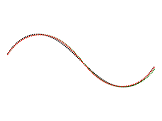
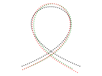
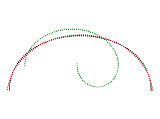
Figure 5: Typical examples of the fairing by the discrete elasticae. Black squares: input curve, green triangles: initial guess, red circles: output elastica.

5 Application: characterization of keylines of Japanese handmade pantiles

5.1 Background and outline

Sangawara (Japanese pantiles) are the most common type of roof tiles in Japan and are thought to be unique to the country. Although the number of buildings with sangawara roofs are decreasing, the landscapes with the remaining constructions having sangawara roofs are consider by the community to be one of the most beautiful scenes and culturally Japanese. Traditionally, sangawara were handmade from local clay by placing a clay plate on a wooden mold, beating it with a board called tataki, and stroking it with a board called nadeita (Figure 6). In recent times, they are mass-produced by metal mold presses in limited areas. The mold shapes are thought to be based on the shape of the sangawara in the handmade era, but companies keep their designs a trade secret, so it is not clear. We consider that it is important to characterize aesthetically pleasing curves like sangawara with mathematical formulas to be used in architectural design. Because of this, and the fact that the process involves bending the clay plate, we thought that the shape of sangawara could possibly be approximated by elasticae. In Section 5.2 we explain how the handmade sangawara (simply referred to as pantiles) were collected, in Section 5.3 we obtain the keyline of each pantile, and in Section 5.4 we approximate those keylines to discrete elasticae.

Figure 6: Beating (left) and stroking (right) in making handmade pantiles in demonstration class at Department of Architecture, Mukogawa Women’s University.

5.2 Generation of 3D keyline data of pantiles

The pantiles we measured had been used in a house built around 1900 in Settsu City, Osaka Prefecture (Figure 7). From the characteristic shapes of the pantiles, they were likely used from the original construction or replaced before the revision of the urban building law in 1924 after the Great Kanto Earthquake. According to the owners, most of the tiles were blown away when the 2nd Muroto Typhoon hit in 1961, so they were collected and re-roofed. After that, only a few of the pantiles were replaced before the house was demolished in March 2017.

In our survey before the demolition, we found that the roofs of this house were covered by four different sizes of pantiles that ranged from 240 to 280 mm in working width. Prior to dismantling the building, we preserved six rows of pantiles (A to F in Figure 8) that covered those four sizes. The pantiles varied in shape due to their handmade nature, so we preserved six rows instead of only four individual pantiles. We measured 37 pantiles of the C and F with a working width of 270 mm (the most commonly used on this house), excluding the eave pantiles (C01, F01).

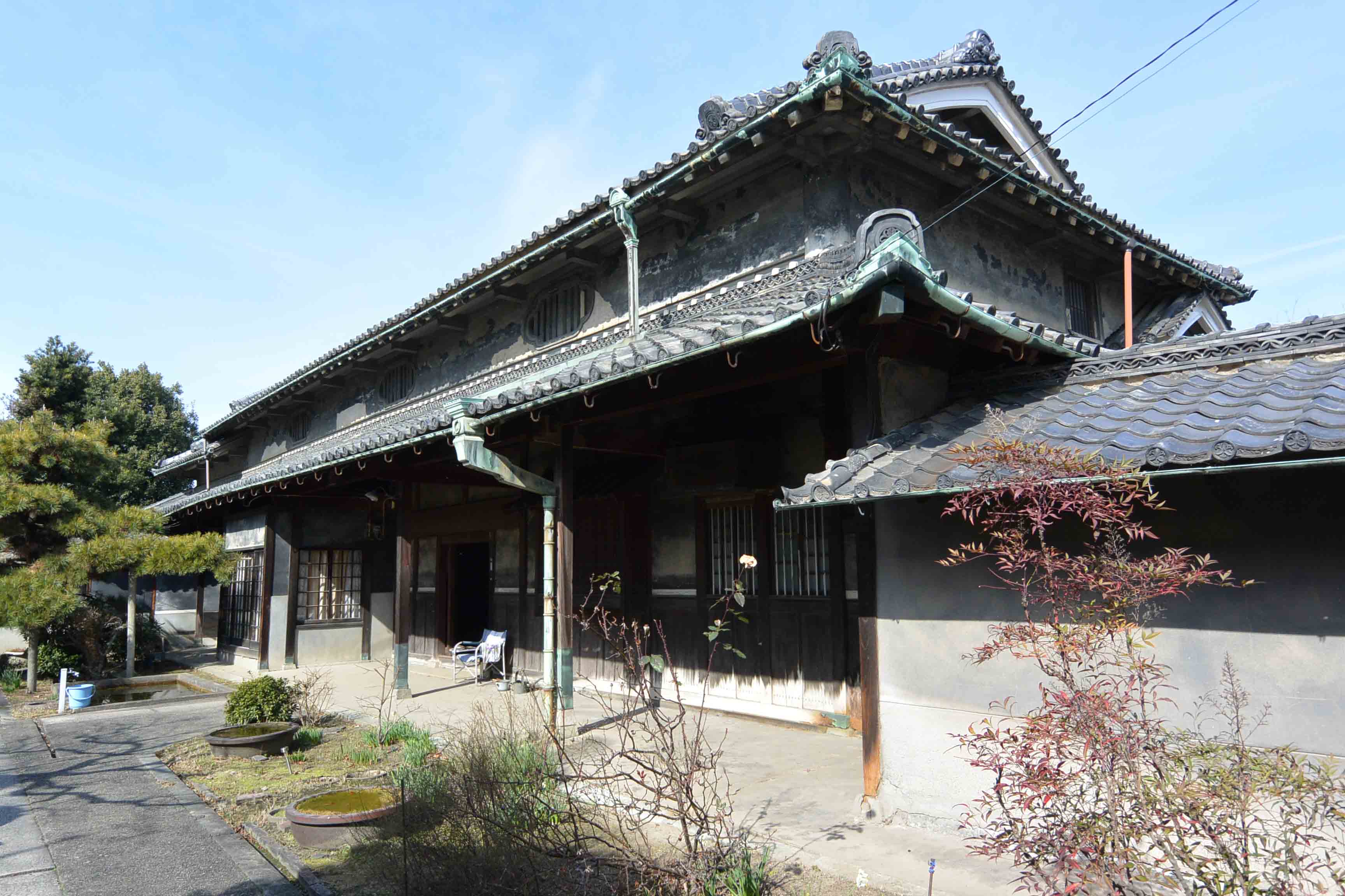
Figure 7: Exterior photos of house with pantile roofs.

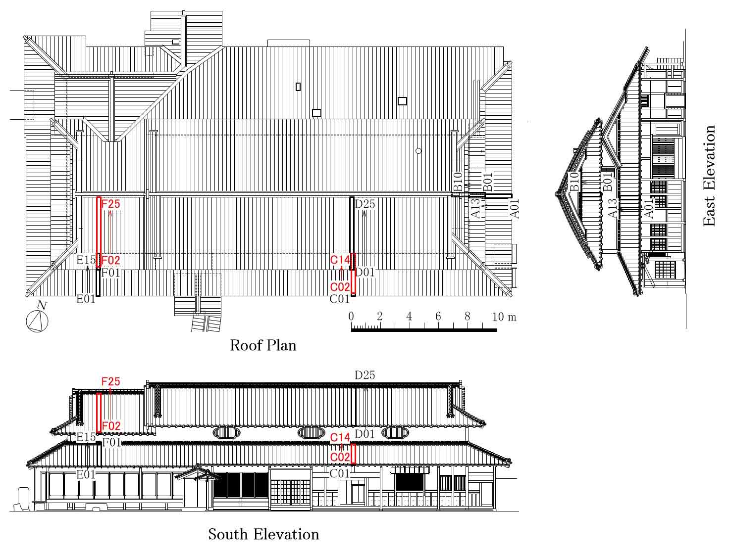
Figure 8: Preserved pantiles (black and red: A-F) and measured pantiles (red: C02-14, F02-25).

We used the NextEngine’s Ultra HD 3D laser scanner and placed it and the pantiles as shown in Figure 9 for the measurements.

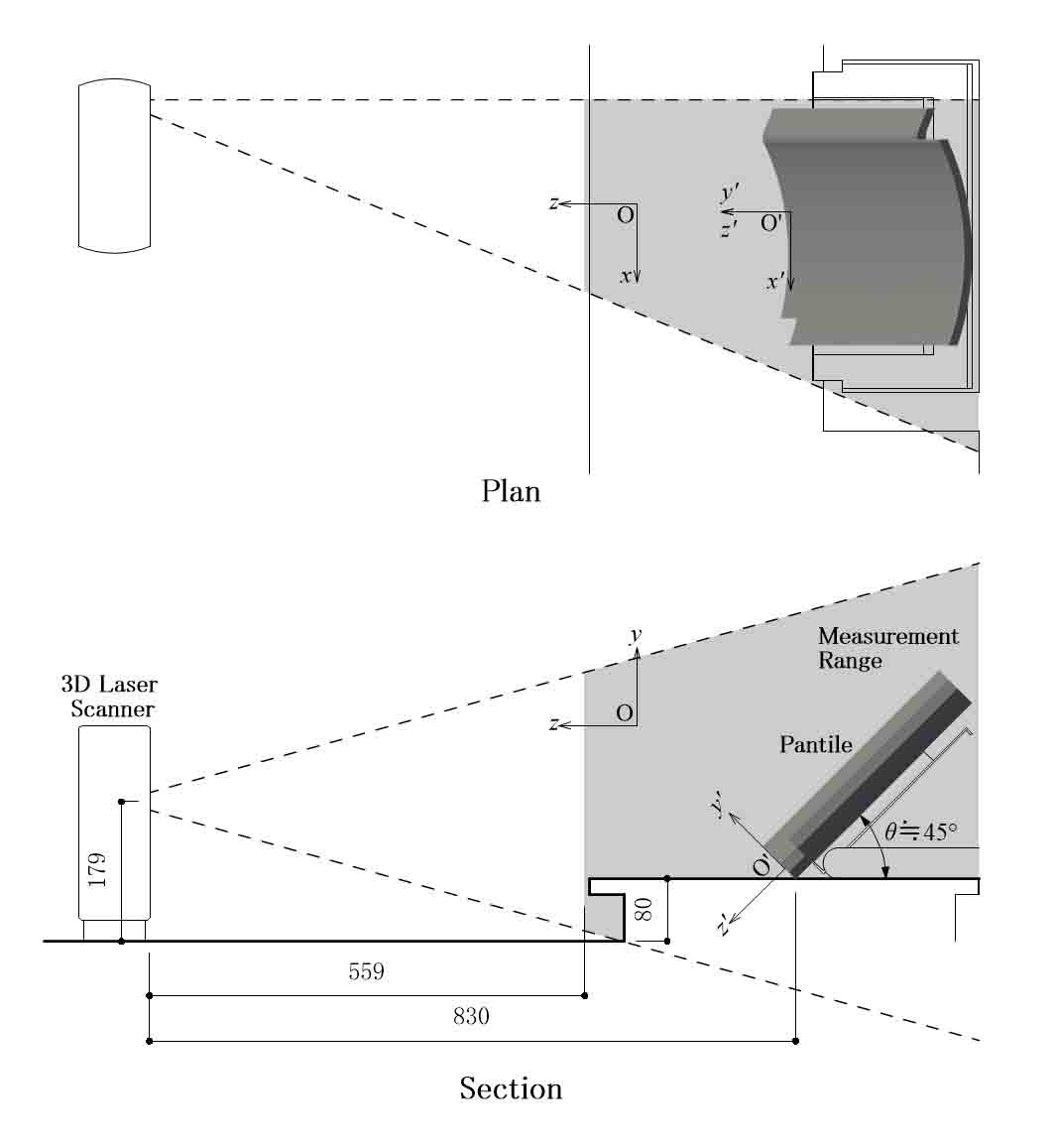
Figure 9: Placement of 3D laser scanner and pantile during measurement.

The mesh data obtained from the 3D laser scanner was read by 3D Systems’ RapidWorks 64 4.1.0 reverse modeling software. We used this software to synthesize and decimate its polygons finer than the scanner’s measurement accuracy (0.3 mm) and then automatically heal incorrect data and fill holes in the meshes.

The two front edges are the 3D keylines of the pantile that could be observed when pitched. The lower edge could be generated by extracting the outer boundary curve of the mesh with RapidWorks. The upper edge could be generated by extracting the curve network from the mesh data with RapidWorks. Figure 10 shows an example of the two 3D keylines (upper and lower edges) generated. Each of these 3D keylines form an open polygon.

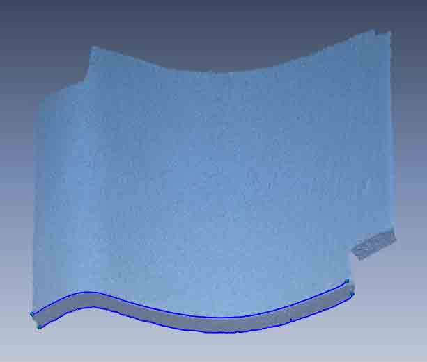
Figure 10: Example of 3D keylines generated (C07).

5.3 Generation and conversion of 2D keylines

Plane fitting of 3D keyline by principal component analysis

In order to generate 2D keyline data from the 3D keylines obtained from the scanning data, we need plane fitting of the 3D data. This can be done by projecting the points in $\mathbb{R}^{3}$ on the plane which minimizes the sum of squared distances from the points. As is well-known, such plane is constructed by applying the principal component analysis of the so-called the covariance matrix. More concretely, let $p_{1},p_{2},\dots,p_{m}\in\mathbb{R}^{3}$ be three-dimensional column vectors that represent spatial coordinates of a point cloud consisting of $m$ points. Their center of gravity $\bar{p}$ is given by

$$\bar{p}=\frac{1}{m}\sum_{k=1}^{m}p_{k}.$$ (5.1)

We consider the covariance matrix $C$ defined by

$$C=\frac{1}{m}\sum_{k=1}^{m}(p_{k}-\bar{p})\mskip 1.0mu\prescript{\smash{\mathrm{t}\mkern-3.0mu}}{}{\mathstrut(p_{k}-\bar{p})},$$

which is real, symmetric positive semi-definite matrix, and let $e_{1},e_{2},e_{3}$ be orthonormal eigenvectors that correspond to eigenvalues $\lambda_{1},\lambda_{2},\lambda_{3}$ ($\lambda_{1}\geq\lambda_{2}\geq\lambda_{3}\geq 0$) of $C$. Then it is known that the plane $\pi$ that includes $\bar{p}$ and is parallel to $e_{1}$ and $e_{2}$ (i.e., with $e_{3}$ as the normal vector) minimizes the sum of the squared distances from $p_{1},p_{2},\dots,p_{m}$ (see, for example, [1]). Therefore, plane fitting is obtained by projecting $p_{1},p_{2},\dots,p_{m}$ onto $\pi$.

Following this idea, the $xyz$-coordinates of the point sequence consisting of all the vertices of the open polygon that constitutes one 3D keyline are converted into the $x^{\prime}y^{\prime}z^{\prime}$-coordinate system, where the center of gravity of the point sequence is the origin $O^{\prime}$ and the orientations of $e_{1}$, $e_{2}$, and $e_{3}$ are the $x^{\prime}$, $y^{\prime}$ and $z^{\prime}$ axes, respectively. The orientations of $e_{1}$, $e_{2}$, and $e_{3}$ are determined to be those of the $x^{\prime}$, $y^{\prime}$ and $z^{\prime}$ axes shown in Figure 9, respectively. When converting the coordinate $p_{k}$ in the $xyz$-coordinate system into the coordinate $p^{\prime}_{k}$ in the $x^{\prime}y^{\prime}z^{\prime}$-coordinate system,

$$p^{\prime}_{k}=\mskip 1.0mu\prescript{\smash{\mathrm{t}\mkern-3.0mu}}{}{\mathstrut(e_{1}\,e_{2}\,e_{3})}(p_{k}-\bar{p}),$$

is satisfied because $(e_{1}\,e_{2}\,e_{3})$ is an orthogonal matrix.

Equilateral open polygon approximation of 2D keyline

The 2D keylines obtained by projecting the 3D keylines onto the $x^{\prime}y^{\prime}$ planes in the previous paragraph (simply referred to as the 2D keylines before approximation) can be approximated by equilateral open polygons using the following procedure.

First, let the end point on the negative side of the $x^{\prime}$ axis of the 2D keyline before approximation (simply referred to as the left end) be the starting point $A_{1}$ after approximation, and let the point on the keyline whose distance from $A_{1}$ is $r$ (= 1.0 mm) be $A_{2}$. Next, let the point on the same keyline where the distance from $A_{2}$ is $r$ and does not return to the left end ($A_{1}$) be $A_{3}$. In the same way, repeat the operation to let the point whose distance from $A_{k}$ is $r$ and does not return to $A_{k-1}$ be $A_{k+1}$ (Figure 13). However, if there are multiple points that satisfy this condition, let the point on the keyline closer to the right end (the end point on the positive side of the $x^{\prime}$ axis) be $A_{k+1}$ (Figure 13). When the only point that has a distance $r$ from $A_{n}$ is the point that returns to $A_{n-1}$, $A_{n}$ is the stop point of the 2D keyline after approximation (Figure 13). All the points from the start point $A_{1}$ to the stop point $A_{n}$ are connected on the sides to make the 2D keyline after approximation. The 2D keyline after approximation is an equilateral open polygon with $n$ vertices, $n-1$ sides, and $r(n-1)=n-1$ mm in total length.

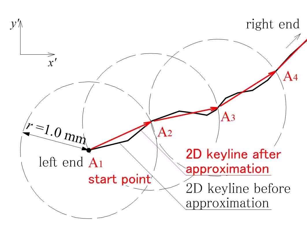
Figure 11: Procedure for equilateral open polygon approximation of 2D keyline (C07 lower keyline).

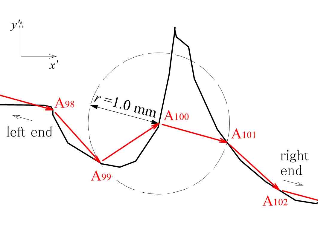
Figure 12: Method of determining vertex of equilateral open polygon when there are multiple points whose distance is r (C07 lower keyline).

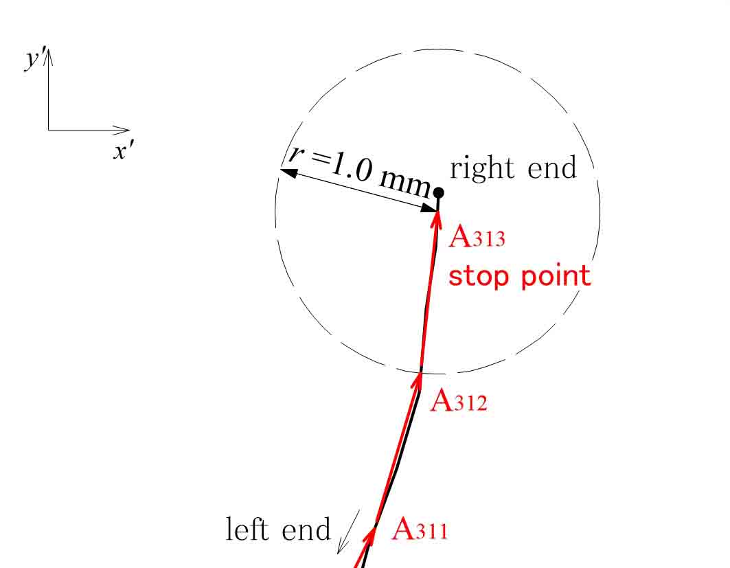
Figure 13: Method of determining stop point of equilateral open polygon (C07 lower keyline).

Coordinate conversion of 2D keylines after approximation by principal component analysis

When measuring the pantiles as shown in Figure 9, we place them one by one on the table by hand. Therefore, the position and rotation angle of each pantile is slightly different. To compare the curves of the keylines of the measured pantiles, we have to eliminate the effects of the positions and rotation angles and convert them into a coordinate system determined by only the keyline shape. This effect is already eliminated by conversion from the $xyz$-coordinate system into the $x^{\prime}y^{\prime}$-coordinate system, where the center of gravity of the point sequence consisting of all the vertices of the 2D keyline is $O^{\prime}$, the orientation of its first principal component is the $x^{\prime}$ axis, and the orientation of its second principal component is the $y^{\prime}$ axis. However, the number and position of the points that compose the point sequence have been changed due to the equilateral open polygon approximation. Therefore, the center of gravity of the point sequence consisting of all vertices of the approximated 2D keyline does not generally coincide with $O^{\prime}$, nor does the orientation of its first principal component coincide with the $x^{\prime}$ axis, nor does the orientation of its second principal component coincide with the $y^{\prime}$ axis. Because the relationship between the shape of the keyline and the coordinate system has been lost, the coordinate system must be converted again into one determined solely by the shape of the keyline. Therefore, by performing the principal component analysis again on the point sequence consisting of all the vertices of the 2D keyline after approximation, we convert the coordinates into the $x^{\prime\prime}y^{\prime\prime}$-coordinate system with the center of gravity of the point sequence as $O^{\prime\prime}$ and the first principal component as the $x^{\prime\prime}$ axis. In the $x^{\prime}y^{\prime}$-coordinate system, let $q_{1},q_{2},\dots,q_{n}$ be the two-dimensional column vectors that represent the plane coordinates of the $n$ points of the 2D keyline after approximation. Then their center of gravity $\bar{q}$ is given by

$$\bar{q}=\frac{1}{n}\sum_{k=1}^{n}q_{k}.$$

Let $f_{1},f_{2}$ be normalized eigenvectors that correspond to the eigenvalues $\mu_{1},\mu_{2}$ ($\mu_{1}\geq\mu_{2}$) of covariance matrix $D$ defined by

$$D=\frac{1}{n}\sum_{k=1}^{n}(q_{k}-\bar{q})\mskip 1.0mu\prescript{\smash{\mathrm{t}\mkern-3.0mu}}{}{\mathstrut(q_{k}-\bar{q})}.$$

Here, the directions of $f_{1}$ and $f_{2}$ are determined so that the diagonal components of $(f_{1}\,f_{2})$ are all positive. When converting the coordinate $q_{k}$ in the $x^{\prime}y^{\prime}$-coordinate system into the coordinate $q^{\prime}_{k}$ in the $x^{\prime}y^{\prime}z^{\prime}$-coordinate system,

$$q^{\prime}_{k}=\mskip 1.0mu\prescript{\smash{\mathrm{t}\mkern-3.0mu}}{}{\mathstrut(f_{1}\,f_{2})}(q_{k}-\bar{q}),$$

is satisfied because $(f_{1}\,f_{2})$ is an orthogonal matrix.

In the following, the $x^{\prime\prime}y^{\prime\prime}$-coordinates obtained by this coordinate conversion will be redefined as $xy$-coordinates.

Estimation of inflection point of approximate curve of 2D keyline

The approximate curve of the 2D keyline of the pantile has one global inflection point and is clearly asymmetric across the inflection point. In general, it is difficult to formulate such a curve in terms of a single elastica. Therefore, we estimate the global inflection point of the approximate curve, then we divide the curve on both sides of the inflection point and approximate them with different elastic curves. We estimate the inflection point using a method inspired by the Ramer-Douglas-Peucker (RDP) algorithm [6, 28], which was devised to simplify an open polygon with many vertices by thinning out the vertices (Figure 14). We call this the RDP method:

1. Among the vertices of the open polygon, let the point farthest from the line segment connecting the two end points be 3. Let the end point on the side with the inflection point (viewed from point 3) be 2, and let the end point on the side without the inflection point be 1.

2. Among the vertices of the open polygon between points 2 and 3, let the point farthest from line segment 2-3 be 4.

3. Among the vertices of the open polygon between the points $P$ ($P=3,4,5,\dots$) and $P+1$, repeat the calculation to let the point farthest from the line segment $P$($P+1$) be $P+2$. However, the numbers of point $P$ and point $P+1$ are switched and the next calculation is performed if point $P+1$ is the upper side of line segment ($P-1$)$P$ and point $P+2$ is also the upper side of line segment $P$($P+1$), or, conversely, if point $P+1$ is the lower side of line segment ($P-1$)$P$ and point $P+2$ is also the lower side of line segment $P$($P+1$).

4. When points $P+1$ and $P+2$ become adjacent vertices on the open polygon, the calculation is terminated and the inflection point is estimated to be $P+2$.

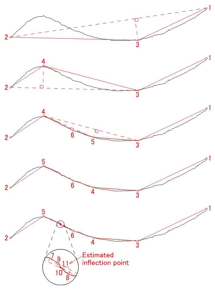
Figure 14: Example of inflection point estimation by RDP method (C07 lower keyline). In the first three curves we apply steps (1), (2) and (3), respectively. In the fourth and fifth curves, following step (3), we switch point 4 to point 5, and point 7 to point 11, respectively. Finally, in the augmented image at the bottom, following step (4), the inflection point is estimated to be point 11.

Because the RDP algorithm is intended to thin out the vertices, its calculation is terminated when an error falls within a certain range. However, the RDP method in this study is meant to estimate the inflection points. Therefore, we repeat the calculation only in the section where the inflection point is estimated to exist until it agrees with the original open polygon, and we estimate the converged point to be the inflection point.

5.4 Approximation of 2D keyline by discrete elastica

For the right (valley) sides of the inflection points of the 37 lower keylines (Figure 15) of the 37 pantiles, we tried to approximate the discrete elastica by the method already described. Among $p=(x_{0},y_{0},h,\phi,z,q,k)$ shown in (4.5), $(x_{0},y_{0})$ were set as the inflection point to allow the discrete elastica to pass through the inflection point after approximation, and the remaining five parameters were optimized. An example of approximation of a keyline of a pantile (C07 lower keyline) by discrete elastica is shown in Figure 16, the calculation results of the 37 approximated discrete elasticae are shown in Figure 17, and the calculation results of the parameters $h$, $\phi$, $z$, $q$, $k$ are shown in Table 1.

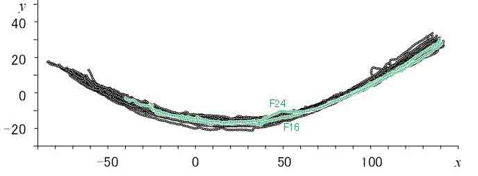
Figure 15: Right (valley) sides of 2D lower keylines for calculation.

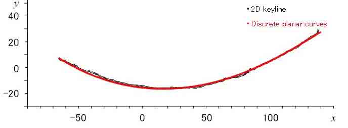
Figure 16: Example approximation by discrete elastica (C07 lower keyline).

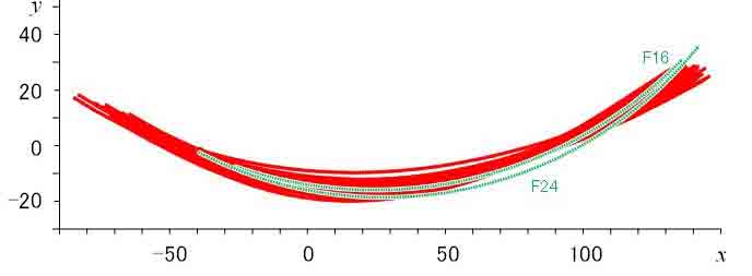
Figure 17: Calculation results of approximated discrete elasticae of 2D lower keylines.

Lower keylines right (valley) side		$h$	$\phi$		$z$	$q$	$k$
		[mm]	[rad]	[grad]
C02–14, F02–15, 17–23, 25	mean	$0.964$	$-0.168$	$-9.623$	$9.001\times 10^{-3}$	$5.919$	$0.353$
	std. dev.	$6.564\times 10^{-3}$	$2.078\times 10^{-3}$	$0.119$	$1.263\times 10^{-3}$	$1.789\times 10^{-3}$	$1.235\times 10^{-2}$
F16		$0.945$	$2.045$	$117.192$	$67.36$	$5.226$	$27.43$
F24		$1.007$	$2.478$	$141.986$	$121.8$	$28.28$	$27.39$

Table 1: Calculation results for $h$, $\phi$, $z$, $q$ and $k$ (mean and standard deviation). Because the values for F16 and F24 were extremely different from the others, the means and standard deviations were calculated for the 35 keylines except for F16 and F24, and the values for F16 and F24 were written separately.

As Table 1 shows, the 35 key lines (except for F16 and F24) show very little variation in the calculated results of the parameters, and the discrete elasticae are similar in both shape and rotation angle. The $k$ values are close to $0.3$, and the shapes are close to sine curves. However, the values of $\phi$, $z$, $q$ and $k$ for F16 and F24 are extremely different from the others. The $k$ values exceed 10, and the shapes are close to arcs.

Figure 18 shows the 37 translated discrete elasticae shown in Figure 17 with the inflection point $(x_{0},y_{0})$ at the origin. The variations of the discrete elasticae are larger than that in Figure 17, suggesting that a certain number of variations and errors may be included in the estimations of the inflection points. In F16 and F24 in particular, the estimated inflection points are located closer to the right (valley) sides. Therefore, we can assume that the areas around the inflection points where the curvature is small are largely omitted, and the discrete elasticae are approximated to be close to the arcs. The effect the local unevenness of the keyline has on the estimation of the inflection point should be examined.

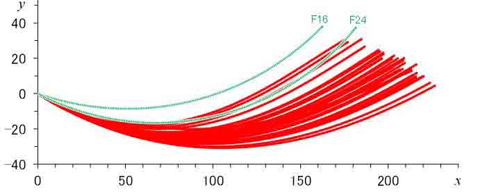
Figure 18: Result of translating discrete elasticae in Figure 17 so that each inflection point is at origin. Calculation results of F16 and F24 are clearly quite different from others.

In conclusion, we found that 35 of the 37 lower keylines of the handmade pantiles could be approximated by discrete elasticae with a very small variation on the right (valley) side of the inflection point. However, the errors of the estimated positions of the inflection points may affect the accuracy of the approximations.

References

- [1] J. Berkmann and T. Caelli, Computation of surface geometry and segmentation using covariance techniques, IEEE PAMI 16(1994) 1114–1116.
- [2] A. Bobenko and U. Pinkall, Discrete surface with constant negative Gaussian curvature and the Hirota equation, J. Differential Geom. 43 (1996) 527–611.
- [3] A. I. Bobenko, Yu. B. Suris, Discrete Time Lagrangian Mechanics on Lie Groups, with an Application to the Lagrange Top, Commun. Math. Phys. 204(1999) 147–188.
-
[4]
A. Bobenko, Geometry II – Discrete Differential Geometry (May 31, 2007), available at:
http://page.math.tu-berlin.de/~techter/lecture notes/geometry2 lecture notes.pdf - [5] D. Brander, J. Gravesen and T. B. Nørbjerg, Approximation by planar elastic curves, Adv. Comput. Math. 43(2017) 25–43.
- [6] D. Douglas and T. Peucker, Algorithms for the reduction of the number of points required to represent a digitized line or its caricature, The Canadian Cartographer 10 (1973) 112–122.
- [7] J. Fernández, S. Graiff Zurita and S. Grillo, Error analysis of forced discrete mechanical systems, Manuscript submitted to AIMS’ Journals (2020)
- [8] R.E. Goldstein and D.M. Petrich, The Korteweg-de Vries hierarchy as dynamics of closed curves in the plane, Phys. Rev. Lett. 67 (1991) 3203–3206.
- [9] R. Hirota, Discretization of the potential modified KdV equation, J. Phys. Soc. Jpn. 67 (1998) 2234–2236.
- [10] R. Hirota, Nonlinear partial difference equations. III. Discrete sine-Gordon equation, J. Phys. Soc. Jpn. 43(1977) 2079–2086.
- [11] T. Hoffmann and N. Kutz, Discrete Curves in and the Toda Lattice, Stud. in Appl. Math. 113(2004) 31–55.
- [12] T. Hoffmann, Discrete Differential Geometry of Curves and Surfaces, MI Lecture Notes 18 (Kyushu University, Fukuoka, 2009).
- [13] J. Inoguchi, K. Kajiwara, N. Matsuura and Y. Ohta, Motion and Bäcklund transformations of discrete planar curves, Kyushu J. Math. 66(2012) 303–324.
- [14] J. Inoguchi, K. Kajiwara, N. Matsuura and Y. Ohta, Discrete mKdV and discrete sine-Gordon flows on discrete space curves. J. Phys. A: Math. Theoret. 47(2014) 235202.
- [15] K. Kajiwara, Y. Ohta, J. Satsuma, B. Grammaticos and A. Ramani, Casorati determinant solutions for the discrete Painlevé-II equation, J. Phys. A: Math. Gen. 27(1994) 915–922.
- [16] K. Kajiwara, M. Noumi and Y. Yamada, Geometric Aspects of Painlevé equations, J. Phys. A: Math. Theor. 50 (2017) 073001 (164pp).
- [17] D. F. Lawden, Elliptic Functions and Applications, Applied Mathematical Sciences, vol. 80. Springer-Verlag, New York (1989)
- [18] J. E. Marsden and T. S. Ratiu, Introduction to mechanics and symmetry, Second ed., Texts in Applied Mathematics, vol. 17 (Springer-Verlag, New York, 1999).
- [19] S. Matsutani, S. Euler’s Elastica and Beyond. J. Geom. Symmetry Phys. 17 (2010) 45–86.
- [20] N. Matsuura, Discrete KdV and discrete modified KdV equations arising from motions of planar discrete curves, Int. Math. Res. Notices, 43 (2011) rnr080 (18 pages).
- [21] N. Matsuura, An explicit formula for discrete planar elastic curves, a talk given at the Annual Meeting of Mathematical Society of Japan (March 18, 2020) (in Japanese).
-
[22]
E.M. McMillan,
Some thoughts on stability in nonlinear periodic focusing systems,
UCRL-17795 (1967). Available at:
https://escholarship.org/uc/item/8zq4t2pc - [23] D. Mumford, Elastica and computer vision, Algebraic Geometry and Its Applications (West Lafayette, IN, 1990), (Springer, New York, 1994) pp. 491–506.
- [24] NIST Digital Library of Mathematical Functions, https://dlmf.nist.gov/ .
- [25] G. W. Patrick, C. Cuell, Error analysis of variational integrators of unconstrained Lagrangian systems, Numer. Math. 113 (2009) 243–-264.
- [26] G.R.W. Quispel, J.A.G. Roberts and C.J. Thompson, Integrable mappings and soliton equations, Phys. Lett. A126(1988) 419–421.
- [27] A. Ramani, B. Grammaticos, and J. Hietarinta, Discrete versions of the Painlevé equations, Phys. Rev. Lett. 67(1991) 1829–1832.
- [28] U. Ramer, An iterative procedure for the polygonal approximation of plane curves, Comput. Graph. Image Process. 1 (1972) 244–256.
- [29] David A. Singer, Lectures on elastic curves and rods, Curvature and variational modeling in physics and biophysics, AIP Conf. Proc. 1002 (2008) 3–32.
- [30] K. Sogo, Variational discretization of Euler’s elastica problem, J. Phys. Soc. Jpn. 75 (2006) 064007.
- [31] D. Takahashi, T. Tokihiro, B. Grammaticos, Y. Ohta and A. Ramani, Constructing solutions to the ultradiscrete Painlevé equations J. Phys. A: Math. Gen. 30 (1997) 7953–7966.
- [32] A. Wächter and L.T. Biegler, On the implementation of an interior-point filter line-search algorithm for large-scale nonlinear programming, Math. Program., Ser. A 106 (2006) 25–57.