Cluster Algebras and Scattering Diagrams
 
Part III
Cluster Scattering Diagrams

Abstract

This is a self-contained exposition of several fundamental properties of cluster scattering diagrams introduced and studied by Gross, Hacking, Keel, and Kontsevich. In particular, detailed proofs are presented for the construction, the mutation invariance, and the positivity of theta functions of cluster scattering diagrams. Throughout the text we highlight the fundamental roles of the dilogarithm elements and the pentagon relation in cluster scattering diagrams.

[depth=2]

0.0 Introduction to Part III

This is a self-contained exposition of several fundamental properties of cluster scattering diagrams (CSDs for short) introduced and studied by Gross, Hacking, Keel, and Kontsevich [GHKK18].

Scattering diagrams originated in the study of homological mirror symmetry, and they are developed in the works of Kontsevich-Soibelman [KS06, KS08, KS14], Gross-Siebert [GS11], Gross-Pandharipande-Siebert [GPS10], Gross [Gro11], Carl-Pumperla-Siebert [CPS], etc. The connection to cluster algebras was established by Gross-Hacking-Keel-Kontsevich [GHKK18], where CSDs were introduced. Then, with a scattering diagram technique, several important conjectures on cluster algebras were proved.

Here is a brief description of the contents.

• In the first half (Sections 1–3) we present a construction of CSDs without assuming any knowledge on scattering diagrams. The main result here is the existence and the uniqueness of a CSD for a given seed (Theorem 0.3.12).

• In the second half (Sections 4–7) we present the fundamental properties of CSDs, which are necessary to prove several conjectures in cluster algebras, including

  • the mutation invariance (Theorem 0.6.9),

  • the positivity of theta functions (Theorems 0.5.2 and 0.7.9).

• We present detailed proofs for all propositions in a self-contained way.

The connection between CSDs and cluster patterns are given in Part II based on the above results. Thus, this part is regarded as a supplement to Part II. Also, it may be read independently as an introductory text to CSDs.

While the most results are taken from [GHKK18, KS14], there are several added or modified proofs and new results due to us. Most notably, we employ the following approach, which adds novelty to our presentation:

• We clearly separate the structure group of walls and its faithful representation (the principal $x$-representation) employed for the construction of CSDs in [GHKK18]. In the first half we only use the structure group itself. This enables us to lift the assumption of the nondegeneracy for the fixed data in [GHKK18], thereby makes the construction of CSDs more transparent. In the second half we apply the principal $x$-representation to the wall elements when needed.

• Throughout we highlight the fundamental role of the dilogarithm elements and the pentagon relation in CSDs, which is implicit in [GHKK18].

More recently, the quantum CSDs were studied by Davison-Mandel [DM21], where the counterparts of many results presented here were given.

0.1 Underlying algebraic structure

In this section we introduce some underlying algebraic structure behind scattering diagrams we are going to study.

0.1.1 Fixed data and seed

Definition 0.1.1 (Fixed data).

A fixed data $\Gamma$ consists of the following:

• A lattice $N\simeq\mathbb{Z}^{r}$ of rank $r$ with a skew-symmetric bilinear form

  $$\{\cdot,\cdot\}:N\times N\rightarrow\mathbb{Q}.$$ (0.1.1)

• A sublattice $N^{\circ}\subset N$ of finite index (equivalently, of rank $r$) such that

  $$\{N^{\circ},N\}\subset\mathbb{Z}.$$ (0.1.2)

• Positive integers $\delta_{1},\dots,\delta_{r}$ such that there is a basis $(e_{1},\dots,e_{r})$ of $N$, where $(\delta_{1}e_{1},\dots,\delta_{r}e_{r})$ is a basis of $N^{\circ}$.

• $M=\mathrm{Hom}(N,\mathbb{Z})$, $M^{\circ}=\mathrm{Hom}(N^{\circ},\mathbb{Z})$.

We say that $\Gamma$ is nondegenerate (resp. degenerate) if $\{\cdot,\cdot\}$ is nondegenerate (resp. degenerate).

For a given $N^{\circ}\subset N$ of finite index, the above $\delta_{1},\dots,\delta_{r}$ always exist; for example, take the elementary divisors of the embedding $N^{\circ}\hookrightarrow N$. However, other choices are equally good.

Let $M_{\mathbb{R}}=M\otimes_{\mathbb{Z}}\mathbb{R}\simeq\mathbb{R}^{r}$, and we regard

$$M\subset M^{\circ}\subset M_{\mathbb{R}}.$$ (0.1.3)

Let $\langle\cdot,\cdot\rangle:N^{\circ}\times M^{\circ}\rightarrow\mathbb{Z}$ be the canonical paring. We also write its linear extension $N\times M_{\mathbb{R}}\rightarrow\mathbb{R}$ by the same symbol.

Definition 0.1.2 (Seed).

A seed $\mathfrak{s}=(e_{1},\dots,e_{r})$ for a fixed data $\Gamma$ is a basis of $N$ such that $(\delta_{1}e_{1},\dots,\delta_{r}e_{r})$ is a basis of $N^{\circ}$.

For a seed $\mathfrak{s}$ for $\Gamma$, we have a basis $(e_{1}^{*}$, …, $e_{r}^{*})$ of $M$ that is dual to $(e_{1},\dots,e_{r})$. Let $f_{i}=e^{*}_{i}/\delta_{i}$. Then, we also have a basis $(f_{1},\dots,f_{r})$ of $M^{\circ}$ that is dual to the basis $(\delta_{1}e_{1},\dots,\delta_{r}e_{r})$ of $N^{\circ}$.

Let $\Omega=\Omega_{\Gamma,\mathfrak{s}}=(\omega_{ij})$ be the $r\times r$ skew-symmetric rational matrix defined by $\omega_{ij}=\{e_{i},e_{j}\}$, and let $\Delta=\Delta_{\Gamma,\mathfrak{s}}=\mathrm{diag}(\delta_{1},\dots,\delta_{r})$ be the diagonal matrix with diagonal entries $\delta_{1},\dots,\delta_{r}$. Let $B=B_{\Gamma,\mathfrak{s}}=(b_{ij})$ be the $r\times r$ integer matrix defined by

$$B=\Delta\Omega,\quad b_{ij}=\{\delta_{i}e_{i},e_{j}\}.$$ (0.1.4)

Since $\Omega=\Delta^{-1}B$ is skew-symmetric, $B$ is skew-symmetrizable with a (left) skew-symmetrizer $D=\Delta^{-1}$ in the sense of [FZ02].

Conversely, for any $r\times r$ skew-symmetrizable integer matrix $B=(b_{ij})$, there is a (not unique) decomposition

$$B=\Delta\Omega,$$ (0.1.5)

where $\Delta=\mathrm{diag}(\delta_{1},\dots,\delta_{r})$ with positive integers $\delta_{1},\dots,\delta_{r}$ and $\Omega=(\omega_{ij})$ is an $r\times r$ skew-symmetric rational matrix. Then, we set

$$N=\bigoplus_{i=1}^{r}\mathbb{Z}e_{i},\quad\{e_{i},e_{j}\}=\omega_{ij},\quad N^{\circ}=\bigoplus_{i=1}^{r}\mathbb{Z}\delta_{i}e_{i}.$$ (0.1.6)

This yields a (not unique) pair of a fixed data $\Gamma$ and a seed $\mathfrak{s}$ such that $B$ is given by (0.1.4).

The seed $\mathfrak{s}$ here is identified with the initial seed $(\mathbf{x},\mathbf{y},B)$ for a cluster pattern or a cluster algebra in the sense of [FZ07] with

$$x_{i}=x^{f_{i}},\quad y_{i}=y^{e_{i}},\quad b_{ij}=\{\delta_{i}e_{i},e_{j}\},$$ (0.1.7)

where $\mathbf{x}=(x_{i})_{i=1}^{r}$, $\mathbf{y}=(y_{i})_{i=1}^{r}$, and $B=(b_{ij})_{i,j=1}^{r}$ are cluster variables ($x$-variables), coefficients ($y$-variables), and an exchange matrix in [FZ07], and $x$ and $y$ are symbols for the formal exponential. See Part II for more details.

Remark 0.1.3.

In (0.1.2) we took the transpose of the bilinear form $\{\cdot,\cdot\}$ in [GHKK18] to match the convention of exchange matrices in [FZ07] in the above correspondence. As a consequence, every expression concerning the bilinear form is the transpose of the one in [GHKK18] throughout Part III.

Let us introduce a group homomorphism

$$\begin{matrix}p^{*}:&N&\rightarrow&M^{\circ}\\ &n&\mapsto&\{\cdot,n\}.\end{matrix}$$ (0.1.8)

By definition, we have

$$\langle n^{\prime},p^{*}(n)\rangle=\{n^{\prime},n\}\in\mathbb{Z}\quad(n^{\prime}\in N^{\circ},n\in N).$$ (0.1.9)

Lemma 0.1.4.

Let $e_{i}$, $f_{i}$, $B=(b_{ij})$ be as above.

(a). We have

$$p^{*}(e_{j})=\sum_{i=1}^{r}b_{ij}f_{i}.$$ (0.1.10)

Thus, the matrix representation of $p^{*}$ with respect to the above bases is given by $B$.

(b). $\Gamma$ is nondegenerate if and only if the matrix $B$ is nonsingular.

(c). The map $p^{*}$ is injective if and only if $\Gamma$ is nondegenerate.

Proof.

(a). One can verify it as

$$\langle\delta_{i}e_{i},p^{*}(e_{j})\rangle=\{\delta_{i}e_{i},e_{j}\}=b_{ij}=\biggl{\langle}\delta_{i}e_{i},\sum_{k=1}^{r}b_{kj}f_{k}\biggr{\rangle}.$$ (0.1.11)

The properties (b) and (c) follow from (a). ∎

Throughout the section, we fix a seed $\mathfrak{s}=(e_{1},\dots,e_{r})$ of a given fixed data $\Gamma$ unless otherwise mentioned.

Let $N^{+}$ be the set of positive elements in $N$ with respect to $\mathfrak{s}$, namely,

$$N^{+}=N_{\mathfrak{s}}^{+}:=\biggl{\{}\sum_{i=1}^{r}a_{i}e_{i}\biggm{|}a_{i}\in\mathbb{Z}_{\geq 0},\ \sum_{i=1}^{r}a_{i}>0\biggr{\}}.$$ (0.1.12)

We say that $n\in N$ is primitive if there is no pair $j\in\mathbb{Z}_{>1}$ and $n^{\prime}\in N$ such that $n=jn^{\prime}$. Let $N_{\mathrm{pr}}^{+}$ be the set of all primitive elements in $N^{+}$.

We have a natural degree function $\deg:N^{+}\rightarrow\mathbb{Z}_{>0}$ given by

$$\deg:\sum_{i=1}^{r}a_{i}e_{i}\mapsto\sum_{i=1}^{r}a_{i}.$$ (0.1.13)

For each integer $\ell>0$, we set

$$(N^{+})^{\leq\ell} =\{n\in N^{+}\mid\deg(n)\leq\ell\},\quad(N_{\mathrm{pr}}^{+})^{\leq\ell}=(N^{+})^{\leq\ell}\cap N_{\mathrm{pr}}^{+},$$ (0.1.14)

$$(N^{+})^{>\ell} =\{n\in N^{+}\mid\deg(n)>\ell\},\quad(N_{\mathrm{pr}}^{+})^{>\ell}=(N^{+})^{>\ell}\cap N_{\mathrm{pr}}^{+},$$ (0.1.15)

$$(N^{+})^{\ell} =\{n\in N^{+}\mid\deg(n)=\ell\},\quad(N_{\mathrm{pr}}^{+})^{\ell}=(N^{+})^{\ell}\cap N_{\mathrm{pr}}^{+}.$$ (0.1.16)

In particular, $(N^{+})^{\leq\ell}$ is a finite set.

0.1.2 Structure group $G$

Let us fix a field $\mathbbm{k}$ of characteristic zero arbitrarily, e.g., $\mathbbm{k}=\mathbb{Q}$.

For a given fixed data $\Gamma$ and a seed $\mathfrak{s}$, we introduce an $N^{+}$-graded Lie algebra $\mathfrak{g}$ over $\mathbbm{k}$ with generators $X_{n}$ ($n\in N^{+}$) as follows:

$$\mathfrak{g}=\mathfrak{g}_{\mathfrak{s}}:=\bigoplus_{n\in N^{+}}\mathfrak{g}_{n},\quad\mathfrak{g}_{n}=\mathbbm{k}X_{n},$$ (0.1.17)

$$[X_{n},X_{n^{\prime}}]=\{n,n^{\prime}\}X_{n+n^{\prime}}.$$ (0.1.18)

The Jacobi identity is easily seen by the following cyclic expression:

$$[X_{n_{1}},[X_{n_{2}},X_{n_{3}}]]=(\{n_{1},n_{2}\}\{n_{2},n_{3}\}-\{n_{2},n_{3}\}\{n_{3},n_{1}\})X_{n_{1}+n_{2}+n_{3}}.$$ (0.1.19)

For each integer $\ell>0$, we define a Lie algebra ideal and a quotient of $\mathfrak{g}$,

$$\mathfrak{g}^{>\ell}:=\bigoplus_{n\in(N^{+})^{>\ell}}\mathfrak{g}_{n},\quad\mathfrak{g}^{\leq\ell}:=\mathfrak{g}/\mathfrak{g}^{>\ell}\simeq\bigoplus_{n\in(N^{+})^{\leq\ell}}\mathfrak{g}_{n}\text{\ (as a vector space)}.$$ (0.1.20)

It is important that $\mathfrak{g}^{\leq\ell}$ is a nilpotent Lie algebra. We have the canonical projections

$$\pi_{\ell^{\prime},\ell}:\mathfrak{g}^{\leq\ell^{\prime}}\rightarrow\mathfrak{g}^{\leq\ell}\quad(\ell^{\prime}>\ell).$$ (0.1.21)

Thus, we have the completion of $\mathfrak{g}$,

$$\widehat{\mathfrak{g}}=\widehat{\mathfrak{g}}_{\mathfrak{s}}:=\lim_{\longleftarrow}\mathfrak{g}^{\leq\ell}\simeq\prod_{n\in N^{+}}\mathfrak{g}_{n}\quad\text{(as a vector space)}$$ (0.1.22)

with the canonical projections $\pi_{\ell}:\widehat{\mathfrak{g}}\rightarrow\mathfrak{g}^{\leq\ell}$ ($\ell>0$).

For any Lie subalgebra $\mathfrak{h}$ of $\mathfrak{g}$, its completion $\widehat{\mathfrak{h}}$ is defined by

$$\mathfrak{h}^{>\ell}=\mathfrak{h}\cap\mathfrak{g}^{>\ell},\quad\mathfrak{h}^{\leq\ell}=\mathfrak{h}/\mathfrak{h}^{>\ell},\quad\widehat{\mathfrak{h}}=\lim_{\longleftarrow}\mathfrak{h}^{\leq\ell}.$$ (0.1.23)

Next, we define the exponential group $G$ for the Lie algebra $\widehat{\mathfrak{g}}$ in (0.1.22). In fact, there are two equivalent ways to define it.

(a). For each nilpotent Lie algebra $\mathfrak{g}^{\leq\ell}$ in (0.1.20), we define the associated exponential group

$$G^{\leq\ell}=\exp(\mathfrak{g}^{\leq\ell})$$ (0.1.24)

as follows: As a set, $G^{\leq\ell}$ is identified with $\mathfrak{g}^{\leq\ell}$ with $\exp(X)\leftrightarrow X$, and its product is defined by the Baker-Campbell-Hausdorff (BCH) formula (e.g., [Jac79, §V.5]),

$$\begin{split}&\ \exp(X)\exp(Y)\\ =&\ \exp\biggl{(}X+Y+\frac{1}{2}[X,Y]+\frac{1}{12}[X,[X,Y]]-\frac{1}{12}[Y,[X,Y]]+\cdots\biggr{)},\end{split}$$ (0.1.25)

where we do not need the explicit form of the higher order commutators here. Originally, the BCH formula is a product formula for the exponential element $e^{X}=\sum_{k=0}^{\infty}X^{k}/k!$ in the situation where $e^{X}$ makes sense. Here, the product is well-defined due to the nilpotency of $\mathfrak{g}^{\leq\ell}$. Moreover, it is compatible with the canonical projections

$$\pi_{\ell^{\prime},\ell}:G^{\leq\ell^{\prime}}\rightarrow G^{\leq\ell}\quad(\ell^{\prime}>\ell).$$ (0.1.26)

Thus, by the inverse limit we obtain a group

$$G=G_{\mathfrak{s}}=G_{\Gamma,\mathfrak{s}}:=\lim_{\longleftarrow}G^{\leq\ell}$$ (0.1.27)

with the canonical projections $\pi_{\ell}:G\rightarrow G^{\leq\ell}$ ($\ell>0$). Let $G^{>\ell}:=\mathrm{Ker}\,\pi_{\ell}$. When we discuss $G^{\leq\ell}$, we often work with elements in $G$ modulo $G^{>\ell}$.

(b). Alternatively, we may directly define

$$G:=\exp(\widehat{\mathfrak{g}}),$$ (0.1.28)

where the infinite sum in the BCH formula (LABEL:3eq:BCH1) makes sense for $\widehat{\mathfrak{g}}$ again due to the nilpotency of $\mathfrak{g}^{\leq\ell}$. An element $\exp(X)$ ($X\in\widehat{\mathfrak{g}}$) is identified with an element $(\exp(\pi_{\ell}(X)))_{\ell=1}^{\infty}$ of $G$ in (0.1.27).

Here we call $G$ the structure group for the forthcoming scattering diagrams. We remark that the group $G$ depends only on $N$, $\{\cdot,\cdot\}$, and $e_{1},\dots,e_{r}$ among the data from $\Gamma$ and $\mathfrak{s}$. In view of the decomposition (0.1.5), they corresponds to the matrix $\Omega$. Thus, one can take a common $G$ for those $(\Gamma,\mathfrak{s})$ where $N$, $\{\cdot,\cdot\}$, and $e_{1},\dots,e_{r}$ (and $\Omega$) are fixed but $N^{\circ}$ and $\delta_{1},\dots,\delta_{r}$ (and $\Delta$) are taken differently.

For any $g=\exp(X)\in G$ and any $c\in\mathbbm{k}$, a power $g^{c}$ of $g$ is defined by

$$g^{c}:=\exp(cX).$$ (0.1.29)

In particular, for any $c\in\mathbb{Q}$, the fractional power $g^{c}$ of $g$ is unambiguously defined.

We may consider an infinite product in $G$ as follows. Suppose that there is a countable and linearly ordered sequence $(g_{i})_{i\in I}$ ($g_{i}\in G$). Suppose that for any $\ell\in\mathbb{Z}_{>0}$, there are only finitely many $i\in I$ such that $\pi_{\ell}(g_{i})\neq\mathrm{id}$. Let $p_{\ell}$ be the product of those $g_{i}$ such that $\pi_{\ell}(g_{i})\neq\mathrm{id}$ along its linear order, say, from left to right. Then, $\lim_{\ell\rightarrow\infty}p_{\ell}$ yields an element in $G$, which is the infinite product ${\prod}_{i\in I}g_{i}$.

Let $\mathfrak{h}$ be any Lie subalgebra of $\mathfrak{g}$, and let $\mathfrak{h}^{\leq\ell}$ and $\widehat{\mathfrak{h}}$ be the ones in (0.1.23). Then, the corresponding subgroup $H$ of $G$ is defined by

$$H^{\leq\ell}:=\exp(\mathfrak{h}^{\leq\ell}),\quad H:=\lim_{\longleftarrow}H^{\leq\ell}=\exp(\widehat{\mathfrak{h}}).$$ (0.1.30)

The following subgroups of $G$ are especially important.

Definition 0.1.5 (Parallel subgroup).

For each $n\in N^{+}_{\mathrm{pr}}$, we define a Lie subalgebra of $\mathfrak{g}$,

$$\mathfrak{g}_{n}^{\parallel}:=\bigoplus_{j>0}\mathfrak{g}_{jn}.$$ (0.1.31)

This is abelian by (0.1.18) and the skew-symmetry of (0.1.1). Then, we have an abelian subgroup $G_{n}^{\parallel}$ of $G$ corresponding to $\widehat{\mathfrak{g}}_{n}^{\parallel}$ as defined in (0.1.30). We call $G_{n}^{\parallel}$ the parallel subgroup of $n$.

From the BCH formula (LABEL:3eq:BCH1), we obtain the Zassenhaus formula [Mag54], which is regarded as the dual of the BCH formula:

$$\begin{split}&\exp(X+Y)\\ =&\exp(X)\exp(Y)\exp\biggl{(}-\frac{1}{2}[X,Y]\biggr{)}\exp\biggl{(}\frac{1}{3}[Y,[X,Y]]+\frac{1}{6}[X,[X,Y]]\biggr{)}\cdots,\end{split}$$ (0.1.32)

where again the explicit form of higher commutators are not necessary, and the infinite product makes sense in $G$. Together with the BCH formula, it also implies the useful formulas

$$\exp(X)\exp(Y) =\exp(Y)\exp(X)\exp([X,Y])C$$ (0.1.33)

$$=\exp(Y)\exp([X,Y])C^{\prime}\exp(X).$$ (0.1.34)

where $C$ and $C^{\prime}$ are (possibly infinite) products of the exponentials of higher commutators of $X$ and $Y$.

0.1.3 Representations of $G$

Let us introduce two kinds of representations of $G$, which build a bridge between scattering diagrams and cluster algebras.

Let us recall some basic facts on derivations [Jac79, §I.2]. Let $A$ be a (not necessarily associative) algebra over $\mathbbm{k}$. A linear map $D:A\rightarrow A$ is a derivation of $A$ if $D(ab)=D(a)b+aD(b)$ holds for any $a,b\in A$. For any derivations $D_{1}$ and $D_{2}$ of $A$, $[D_{1},D_{2}]:=D_{1}D_{2}-D_{2}D_{1}$ is also a derivation. Thus, we have the Lie algebra $\mathrm{Der}(A)$ consisting of all derivations of $A$ called the derivation (Lie) algebra. For a derivation $D$, suppose that the infinite sum $\exp(D)=\sum_{k=0}^{\infty}D^{k}/k!$ is well-defined as a linear map on $A$. Then, $\exp(D)$ is an algebra automorphism of $A$.

(a). $y$-representation. We consider a monoid

$$Q=Q_{\mathfrak{s}}:= \biggl{\{}\sum_{i=1}^{r}a_{i}e_{i}\biggm{|}a_{i}\in\mathbb{Z}_{\geq 0}\biggr{\}}=N^{+}\sqcup\{0\}\subset N.$$ (0.1.35)

Let $\mathbbm{k}[Q]$ be the monoid algebra of $Q$ over $\mathbbm{k}$. Let $J$ be the maximal ideal of $\mathbbm{k}[Q]$ generated by $N^{+}=Q\setminus\{0\}$, and let

$$\mathbbm{k}[[Q]]=\lim_{\longleftarrow}\mathbbm{k}[Q]/J^{\ell}$$ (0.1.36)

be the completion with respect to $J$. We express any element $f\in\mathbbm{k}[[Q]]$ as a formal power series in a symbol $y$ as

$$f=\sum_{n\in Q}c_{n}y^{n}.$$ (0.1.37)

Let $\mathrm{Der}(\mathbbm{k}[[Q]])$ be the derivation algebra of $\mathbbm{k}[[Q]]$.

For each $n\in N^{+}$, we define a derivation $\tilde{X}_{n}$ on $\mathbbm{k}[[Q]]$ by

$$\tilde{X}_{n}(y^{n^{\prime}}):=\{n,n^{\prime}\}y^{n^{\prime}+n}\quad(n^{\prime}\in Q).$$ (0.1.38)

Proposition 0.1.6 (cf. [GHKK18, §1.1]).

The map

$$\begin{matrix}\rho_{y}:&\widehat{\mathfrak{g}}&\rightarrow&\mathrm{Der}(\mathbbm{k}[[Q]])\\ &\displaystyle X=\sum_{n\in N^{+}}c_{n}X_{n}&\mapsto&\displaystyle\tilde{X}=\sum_{n\in N^{+}}c_{n}\tilde{X}_{n},\end{matrix}$$ (0.1.39)

yields a Lie algebra homomorphism, where the sum could be infinite. Moreover, if $\Gamma$ is nondegenerate, it is injective.

Proof.

First, we regard $\rho_{y}$ in (0.1.39) with finite sum as a map $\mathfrak{g}\rightarrow\mathrm{Der}(\mathbbm{k}[Q])$. Then, we have

$$\begin{split}\tilde{X}_{n_{1}}\tilde{X}_{n_{2}}(y^{n})&=\tilde{X}_{n_{1}}(\{n_{2},n\}y^{n+n_{2}})\\ &=(\{n_{1},n\}+\{n_{1},n_{2}\})\{n_{2},n\}y^{n+n_{2}+n_{1}}.\end{split}$$ (0.1.40)

Thus, we obtain

$$\begin{split}[\tilde{X}_{n_{1}},\tilde{X}_{n_{2}}](y^{n})&=\{n_{1},n_{2}\}\{n_{1}+n_{2},n\}y^{n+n_{1}+n_{2}}\\ &=\{n_{1},n_{2}\}\tilde{X}_{n_{1}+n_{2}}(y^{n}).\end{split}$$ (0.1.41)

Therefore, $\rho_{y}:\mathfrak{g}\rightarrow\mathrm{Der}(\mathbbm{k}[Q])$ is a Lie algebra homomorphism. We show that it is extended to the one in (0.1.39). First, we note that $\mathfrak{g}(J^{\ell+1})\subset J^{\ell+2}$. Thus, $\mathfrak{g}$ acts on $\mathbbm{k}[Q]^{\leq\ell}:=\mathbbm{k}[Q]/J^{\ell+1}$. Next, we have $\mathfrak{g}^{>\ell}(\mathbbm{k}[Q])\subset J^{\ell+1}$. Thus, it is extended to the action of $\widehat{\mathfrak{g}}$. Moreover, this action is compatible with projections $\pi_{\ell^{\prime},\ell}:\mathbbm{k}[Q]^{\leq\ell^{\prime}}\rightarrow\mathbbm{k}[Q]^{\leq\ell}$ for $\ell^{\prime}>\ell$. Therefore, $\widehat{\mathfrak{g}}$ acts on $\mathbbm{k}[[Q]]$. If $\{\cdot,\cdot\}$ is non-degenerate, $\tilde{X}_{n}$ ($n\in N^{+}$) in (0.1.38) are linearly independent. Thus, $\rho_{y}$ is injective. ∎

Remark 0.1.7.

The above representation $\rho_{y}$ is equivalent to the direct sum of the adjoint and the trivial representations of $\widehat{\mathfrak{g}}$.

For any $X\in\widehat{\mathfrak{g}}$, let $\tilde{X}:={\rho}_{y}(X)$. We define

$$\mathrm{Exp}(\tilde{X}):=\sum_{k=0}^{\infty}\frac{1}{k!}\tilde{X}^{k}\in\mathrm{GL}(\mathbbm{k}[[Q]]),$$ (0.1.42)

which is well-defined by the same reason in the proof of Proposition 0.1.6. Since $\tilde{X}$ is a derivation, $\mathrm{Exp}(\tilde{X})$ is an algebra automorphism of $\mathbbm{k}[[Q]]$ as we mentioned. Then, we have the following group homomorphism, where we abuse the symbol $\rho_{y}$, for simplicity.

Proposition 0.1.8.

We have a group homomorphism

$$\begin{matrix}\rho_{y}:&G&\rightarrow&\mathrm{Aut}(\mathbbm{k}[[Q]])\\ &\exp(X)&\mapsto&\mathrm{Exp}(\tilde{X}).\end{matrix}$$ (0.1.43)

Moreover, if $\Gamma$ is nondegenerate, it is injective.

Proof.

The map $\rho_{y}$ is a group homomorphism, because the exponential (0.1.42) also satisfies the same BCH formula as mentioned. Suppose that $\Gamma$ is nondegenerate. Let us show that $\rho_{y}$ is injective. Assume that $\mathrm{Exp}(\tilde{X})=\mathrm{id}$. Then, by the action (0.1.38), we have $\tilde{X}=0$. Then, $X=0$ in $\widehat{\mathfrak{g}}$ by the injectivity of $\rho_{y}$ in Proposition 0.1.6. Thus, $\exp(X)=\mathrm{id}$. ∎

The representation $\rho_{y}$ is closely related with the mutations of $y$-variables in (0.1.7) as we will see soon. Thus, we call it the $y$-representation of $G$.

(b). $x$-representation. Here we assume that $\Gamma$ is nondegenerate from the beginning. Then, thanks to Lemma 0.1.4, the map $p^{*}$ in (0.1.8) is injective. In particular, $p^{*}(e_{1})$, …, $p^{*}(e_{r})$ are $\mathbb{Z}$-linearly independent. We define a monoid

$$P=P_{\mathfrak{s}}:= \biggl{\{}\sum_{i=1}^{r}a_{i}p^{*}(e_{i})\biggm{|}a_{i}\in\mathbb{Z}_{\geq 0}\biggr{\}}=p^{*}(Q)\subset M^{\circ}.$$ (0.1.44)

Let $\mathbbm{k}[P]$ the monoid algebra of $P$ over $\mathbbm{k}$, and $\mathbbm{k}[[P]]$ be the completion by the maximal ideal of $\mathbbm{k}[P]$ generated by $P\setminus\{0\}$. (Note that, if $\Gamma$ is degenerate, we cannot define $\mathbbm{k}[[P]]$.) We express any element $f\in\mathbbm{k}[[P]]$ as a formal power series in a symbol $x$ as

$$f=\sum_{m\in P}c_{m}x^{m}.$$ (0.1.45)

Then, in parallel to (0.1.38), for each $n\in N^{+}$, we define a derivation $\tilde{X}_{n}$ on $\mathbbm{k}[[P]]$ by

$$\tilde{X}_{n}(x^{m}):=\langle n,m\rangle x^{m+p^{*}(n)}\quad(m\in P).$$ (0.1.46)

Then, repeating the same argument for $\rho_{y}$, we obtain the following group homomorphism.

Proposition 0.1.9.

Suppose that $\Gamma$ is nondegenerate. Then, we have an injective group homomorphism

$$\begin{matrix}\rho_{x}:&G&\rightarrow&\mathrm{Aut}(\mathbbm{k}[[P]])\\ &\exp(X)&\mapsto&\mathrm{Exp}(\tilde{X}).\end{matrix}$$ (0.1.47)

The representation $\rho_{x}$ is closely related with the mutations of $x$-variables in (0.1.7) as we will see soon. Thus, we call it the $x$-representation of $G$.

Even though a faithful representation of $G$ is desirable in some situation, it is too restrictive to assume that $\Gamma$ is nondegenerate in view of cluster algebra theory. We will treat this problem later in Section 0.4.

0.1.4 Dilogarithm elements and pentagon relation

As an application of the actions of $G$ in the previous subsection, we show a remarkable relation among certain distinguished elements in $G$.

Let $\mathrm{Li}_{2}(x)$ be the Euler dilogarithm [Lew81] defined by

$$\mathrm{Li}_{2}(x):=\sum_{j=1}^{\infty}\frac{x^{j}}{j^{2}}=-\int_{0}^{x}\frac{\log(1-y)}{y}\,dy.$$ (0.1.48)

It has the following key property:

$$x\frac{d}{dx}\left(-\mathrm{Li}_{2}(-x)\right) =\sum_{j=1}^{\infty}\frac{(-1)^{j+1}}{j}x^{j}=\log(1+x).$$ (0.1.49)

Having this in mind, we introduce the following elements of $G$.

Definition 0.1.10 (Dilogarithm element).

For any $n\in N^{+}$, let

$$\Psi[n]:=\exp\Biggl{(}\,\sum_{j=1}^{\infty}\frac{(-1)^{j+1}}{j^{2}}X_{jn}\Biggr{)}\in G_{n_{0}}^{\parallel},$$ (0.1.50)

where $n_{0}\in N^{+}_{\mathrm{pr}}$ is the unique one such that $n=tn_{0}$ for some integer $t>0$. We call $\Psi[n]$ the dilogarithm element for $n$.

Remark 0.1.11.

It is “only formally” expressed as

$$\Psi[n]=\exp(-\mathrm{Li}_{2}(-X_{n})),$$ (0.1.51)

if we interpret $X_{n}^{j}$ as $X_{jn}$. (Caution: $X_{n}^{j}$ and $X_{jn}$ act differently on $\mathbbm{k}[[Q]]$ and $\mathbbm{k}[[P]]$.)

The elements $\Psi[n]$ are introduced because of the following property.

Proposition 0.1.12 (Cf. [GHKK18, Lemma 1.3]).

(a). Under the $y$-representation $\rho_{y}$, $\Psi[n]$ acts on $\mathbbm{k}[[Q]]$ as

$$\Psi[n](y^{n^{\prime}})=y^{n^{\prime}}(1+y^{n})^{\{n,n^{\prime}\}}\quad(n^{\prime}\in Q).$$ (0.1.52)

(b). Suppose that $\Gamma$ is nondegenerate. Then, under the $x$-representation $\rho_{x}$, $\Psi[n]$ acts on $\mathbbm{k}[[P]]$ as

$$\Psi[n](x^{m})=x^{m}(1+x^{p^{*}(n)})^{\langle n,m\rangle}\quad(m\in P).$$ (0.1.53)

Proof.

Since the calculations are parallel, we concentrate on the case (b).

$$\begin{split}\Psi[n](x^{m})&=x^{m}\exp\Biggl{(}\sum_{j>0}\frac{(-1)^{j+1}}{j^{2}}x^{jp^{*}(n)}\langle jn,m\rangle\Biggr{)}\\ &=x^{m}\exp\Biggl{(}\,\sum_{j>0}\frac{(-1)^{j+1}}{j}x^{jp^{*}(n)}\Biggr{)}^{\langle n,m\rangle}\\ &=x^{m}(1+x^{p^{*}(n)})^{\langle n,m\rangle}.\end{split}$$ (0.1.54)

∎

Observe that the calculation in (0.1.54) is parallel to the derivation of the formula (0.1.49) by the power series calculation. The above automorphisms (0.1.52) and (0.1.53) are identified with the automorphism part of the Fock-Goncharov decomposition of mutations of $y$-variables (coefficients) and $x$-variables (cluster variables) in cluster algebras, respectively, in [FG09, §2.1].

The dilogarithm elements are generators of $G$ in the following sense.

Proposition 0.1.13.

The group $G$ is generated by $\Psi[tn]^{c}$ $(n\in N_{\mathrm{pr}}^{+},t\in\mathbb{Z}_{>0},c\in\mathbbm{k})$ admitting the infinite product.

Proof.

By inverting the expression (0.1.50), one can express $\exp(X_{n})$ ($n\in N^{+}$) as an infinite product of $\Psi[tn]^{c}$ ($t\in\mathbb{Z}_{>0}$, $c\in\mathbb{Q}$). ∎

The dilogarithm elements satisfy the following remarkable relations.

Proposition 0.1.14.

Let $n,n^{\prime}\in N^{+}$. The following relations hold in $G$.

(a). If $\{n^{\prime},n\}=0$, for any $c,c^{\prime}\in\mathbbm{k}$,

$$\Psi[n^{\prime}]^{c^{\prime}}\Psi[n]^{c}=\Psi[n]^{c}\Psi[n^{\prime}]^{c^{\prime}}.$$ (0.1.55)

(b). (Pentagon relation [GHKK18, Example 1.14] for $c=1$.) If $\{n^{\prime},n\}=c$ $(c\in\mathbb{Q},c\neq 0)$,

$$\Psi[n^{\prime}]^{1/c}\Psi[n]^{1/c}=\Psi[n]^{1/c}\Psi[n+n^{\prime}]^{1/c}\Psi[n^{\prime}]^{1/c}.$$ (0.1.56)

Proof.

(a). This is clear from (0.1.18). (b). Let us consider the rank 2 sublattice $N^{\prime}$ of $N$ generated by $n$ and $n^{\prime}$. By the assumption $\{n^{\prime},n\}\neq 0$, the form $\{\cdot,\cdot\}$ restricted on $N^{\prime}$ is nondegenerate. Let $G^{\prime}$ be the subgroup of $G$ corresponding to $N^{\prime}$. Similarly, we consider a monoid

$$P^{\prime}= \{ap^{*}(n)+a^{\prime}p^{*}(n^{\prime})\mid a,a^{\prime}\in\mathbb{Z}_{\geq 0}\}\subset M^{\circ}.$$ (0.1.57)

Since the relation (0.1.56) involves only elements in $G^{\prime}$, one can prove it by the $x$-representation of $G^{\prime}$ on $\mathbbm{k}[[P^{\prime}]]$, which is faithful. The left hand side is given by

$$\begin{split}&\quad\ \Psi[n^{\prime}]^{1/c}\Psi[n]^{1/c}(x^{m})\\ &=\Psi[n^{\prime}]^{1/c}(x^{m}(1+x^{p^{*}(n)})^{\langle n,m\rangle/c})\\ &=x^{m}(1+x^{p^{*}(n^{\prime})})^{\langle n^{\prime},m\rangle/c}(1+x^{p^{*}(n)}(1+x^{p^{*}(n^{\prime})}))^{\langle n,m\rangle/c}.\end{split}$$ (0.1.58)

The right hand side is given by

$$\begin{split}&\quad\ \Psi[n]^{1/c}\Psi[n+n^{\prime}]^{1/c}\Psi[n^{\prime}]^{1/c}(x^{m})\\ &=\Psi[n]^{1/c}\Psi[n+n^{\prime}]^{1/c}(x^{m}(1+x^{p^{*}(n^{\prime})})^{\langle n^{\prime},m\rangle/c})\\ &=\Psi[n]^{1/c}(x^{m}(1+x^{p^{*}(n+n^{\prime})})^{\langle n+n^{\prime},m\rangle/c}\\ &\qquad\times(1+x^{p^{*}(n^{\prime})}(1+x^{p^{*}(n+n^{\prime})})^{-1})^{\langle n^{\prime},m\rangle/c})\\ &=\Psi[n]^{1/c}(x^{m}(1+x^{p^{*}(n+n^{\prime})})^{\langle n,m\rangle/c}(1+x^{p^{*}(n+n^{\prime})}+x^{p^{*}(n^{\prime})})^{\langle n^{\prime},m\rangle/c})\\ &=x^{m}(1+x^{p^{*}(n)})^{\langle n,m\rangle/c}(1+x^{p^{*}(n+n^{\prime})}(1+x^{p^{*}(n)})^{-1})^{\langle n,m\rangle/c}\\ &\qquad\times(1+x^{p^{*}(n+n^{\prime})}(1+x^{p^{*}(n)})^{-1}+x^{p^{*}(n^{\prime})}(1+x^{p^{*}(n)})^{-1})^{\langle n^{\prime},m\rangle/c}\\ &=x^{m}(1+x^{p^{*}(n)}+x^{p^{*}(n+n^{\prime})})^{\langle n,m\rangle/c}(1+x^{p^{*}(n^{\prime})})^{\langle n^{\prime},m\rangle/c}.\end{split}$$ (0.1.59)

Thus, two expressions agree. ∎

Remark 0.1.15.

(a). The above calculation for $c=1$ is essentially the same for the pentagon periodicity of $x$-variables for a cluster algebra of type $A_{2}$ in [FZ02]. Alternatively, one can also work with the $y$-representation. Then, the calculation for $c=1$ is essentially the same for the pentagon periodicity of $y$-variables for a cluster algebra of type $A_{2}$ in [FZ02].

(b). The case $c\neq 1$ follows from the case $c=1$ by Proposition 0.1.17.

0.1.5 Equivalence of fixed data and normalization factor

There is some redundancy for choosing a fixed data. Let us start with a simple situation.

Definition 0.1.16 (Rescaling of fixed data).

Let $\Gamma$ and $\Gamma^{\prime}$ be a pair of fixed data. We say that $\Gamma^{\prime}$ is a rescaling of $\Gamma$ if there is some rational number $\lambda>0$ such that the following relations hold:

$$N^{\prime} =N,$$ (0.1.60)

$$\{n_{1},n_{2}\}^{\prime} =\lambda\{n_{1},n_{2}\},$$ (0.1.61)

$$(N^{\circ})^{\prime} =\lambda^{-1}N^{\circ},$$ (0.1.62)

$$\delta^{\prime}_{i} =\lambda^{-1}\delta_{i},$$ (0.1.63)

$$(M^{\circ})^{\prime} =\lambda M^{\circ}.$$ (0.1.64)

The exchange matrix $B$ associated with $(\Gamma,\mathfrak{s})$ in (0.1.4) is invariant under the above rescaling, namely,

$$b^{\prime}_{ij}=\{\delta^{\prime}_{i}e_{i},e_{j}\}^{\prime}=\lambda\{\lambda^{-1}\delta_{i}e_{i},e_{j}\}=b_{ij}.$$ (0.1.65)

Let $\mathfrak{s}=(e_{1},\dots,e_{r})$ be a seed for $\Gamma$. Then, $\mathfrak{s}$ is also regarded as a seed for $\Gamma^{\prime}$. Let $\widehat{\mathfrak{g}}^{\prime}$ and $G^{\prime}$ be the corresponding Lie algebra and group for $\Gamma^{\prime}$ and $\mathfrak{s}$.

Proposition 0.1.17.

We have a Lie algebra isomorphism

$$\begin{matrix}\phi_{\lambda}:&\widehat{\mathfrak{g}}^{\prime}&\rightarrow&\widehat{\mathfrak{g}}\\ &X^{\prime}_{n}&\mapsto&\lambda X_{n}\end{matrix}$$ (0.1.66)

and a group isomorphism

$$\begin{matrix}\phi_{\lambda}:&G^{\prime}&\rightarrow&G\\ &\exp(X^{\prime}_{n})&\mapsto&\exp(\lambda X_{n}).\end{matrix}$$ (0.1.67)

Proof.

This is due to the relation (0.1.61) and the commutation relation (0.1.18). ∎

Definition 0.1.18 (Normalization factor).

For any $n\in N^{+}$, let $\delta(n)$ be the smallest positive rational number such that $\delta(n)n\in N^{\circ}$. We call $\delta(n)$ the normalization factor of $n$ with respect to $N^{\circ}$.

Example 0.1.19.

(a). For the seed $\mathfrak{s}=(e_{1},\dots,e_{r})$ under consideration, we have $\delta(e_{i})=\delta_{i}$.

(b). For any $n\in N^{+}_{\mathrm{pr}}$ and any integer $t>0$, we have

$$\delta(tn)=\delta(n)/t,$$ (0.1.68)

because $\delta(tn)tn=\delta(n)n$. Also, $\delta(n)$ is an integer. Otherwise, let $\delta(n)=r/s$ be the irreducible rational expression with $s\neq 1$. Then, we have $n,(r/s)n\in N$. Thus, $(1/s)n\in N$. This contradicts that $n$ is primitive.

Proposition 0.1.20.

Let $G$ and $G^{\prime}$ be as above. For any $n\in N^{+}_{\mathrm{pr}}$, let $g\in G_{n}^{\parallel}$ and $g^{\prime}\in(G^{\prime})_{n}^{\parallel}$ with

$$g=\exp\Biggl{(}\delta(n)\sum_{j>0}c_{j}X_{jn}\Biggr{)},\quad g^{\prime}=\exp\Biggl{(}\delta^{\prime}(n)\sum_{j>0}c^{\prime}_{j}X^{\prime}_{jn}\Biggr{)},$$ (0.1.69)

where $\delta(n)$ and $\delta^{\prime}(n)$ are the normalization factors with respect to $N^{\circ}$ and $(N^{\circ})^{\prime}$. Then,

$$\phi_{\lambda}(g^{\prime})=g.$$ (0.1.70)

if and only $c_{j}=c^{\prime}_{j}$ for any $j>0$.

Proof.

This follows from (0.1.66) and the transformation of the normalization factors $\delta^{\prime}(n)=\lambda^{-1}\delta(n)$ by (0.1.62). ∎

In view of Proposition 0.1.20, it is natural to express an element $g\in G_{n}^{\parallel}$ as

$$g=g_{0}^{\delta(n)},$$ (0.1.71)

where $g_{0}=g^{1/\delta(n)}$. We call (0.1.71) the normalized form of $g$. Then, the coefficients $c_{j}$ of the expansion $g_{0}=\exp(\,\sum_{j>0}c_{j}X_{jn})$ are invariant under the rescaling of $\Gamma$.

Example 0.1.21.

For $\Psi[n]$ in (0.1.50) with $n=tn_{0}$ therein, we have

$$\phi_{\lambda}(\Psi^{\prime}[n]^{\delta^{\prime}(n_{0})})=\Psi[n]^{\delta(n_{0})}.$$ (0.1.72)

Thus, we also have

$$\phi_{\lambda}(\Psi^{\prime}[n]^{\delta^{\prime}(n)})=\Psi[n]^{\delta(n)}.$$ (0.1.73)

These elements play the main role in the forthcoming CSDs.

Now we consider a more general situation.

Definition 0.1.22.

Let $(\Gamma,\mathfrak{s})$ be a pair of a fixed data and a seed, and let $B_{\Gamma,\mathfrak{s}}$ be the associated matrix in (0.1.4). We say that $(\Gamma,\mathfrak{s})$ and $(\Gamma^{\prime},\mathfrak{s}^{\prime})$ are $B$-equivalent if $B_{\Gamma,\mathfrak{s}}=B_{\Gamma^{\prime},\mathfrak{s}^{\prime}}$.

In Section 0.1.1 we have seen that, for a given skew-symmetrizable matrix $B$, there is a (not unique) pair $(\Gamma,\mathfrak{s})$ such that $B=B_{\Gamma,\mathfrak{s}}$. Let us show that the associated group $G_{\Gamma,\mathfrak{s}}$ is uniquely determined from $B$ up to isomorphism. This fact is natural in view of the correspondence to cluster algebras.

Proposition 0.1.23.

If $(\Gamma,\mathfrak{s})$ and $(\Gamma^{\prime},\mathfrak{s}^{\prime})$ are $B$-equivalent, then the associated groups $G_{\Gamma,\mathfrak{s}}$ and $G_{\Gamma^{\prime},\mathfrak{s}^{\prime}}$ are isomorphic.

Proof.

Let $B=B_{\Gamma,\mathfrak{s}}=B_{\Gamma^{\prime},\mathfrak{s}^{\prime}}$. We say that an $n\times n$ matrix $A$ is indecomposable if there is no pair $I,J\subset\{1,\dots,r\}$, $I\sqcup J=\{1,\dots,r\}$, $I,J\neq\emptyset$ such that $a_{ij}=0$ for any $i\in I$ and $j\in J$. Suppose that $B$ is decomposed into $B_{1}\oplus\cdots\oplus B_{p}$ up to simultaneous permutation of rows and columns, where $B_{i}$ are indecomposable submatrices of $B$. Accordingly, the groups $G=G_{\Gamma,\mathfrak{s}}$ and $G^{\prime}=G_{\Gamma^{\prime},\mathfrak{s}^{\prime}}$ are factorized into the corresponding subgroups $G=\prod_{i=1}^{p}G_{i}$ and $G^{\prime}=\prod_{i=1}^{p}G^{\prime}_{i}$. Thus, we only need to prove the claim when $B$ is indecomposable. Then, it is well known and easy to show that a (left) skew-symmetrizer of $B$ is unique up to a positive rational number. This implies that $\delta_{i}$ and $\delta^{\prime}_{i}$ are related by $\delta^{\prime}_{i}=\lambda^{-1}\delta_{i}$ with a common multiple $\lambda^{-1}$. Let us identify $e_{i}$ with $e^{\prime}_{i}$ ($i=1,\dots,r$) and $N$ with $N^{\prime}$. Now we are in the situation of Definition 0.1.16. Therefore, $G$ and $G^{\prime}$ are isomorphic by Proposition 0.1.17. ∎

The above proof also tells that the parallel results to Proposition 0.1.20 and Example 0.1.21 hold in the situation of Proposition 0.1.23.

0.1.6 Formulas for dilogarithm elements

Let us present some useful formulas for dilogarithm elements.

Proposition 0.1.24.

Let $n,n^{\prime}\in N^{+}$.

(a). ([GHKK18, Lemma C.8].) If $\{\delta(n^{\prime})n^{\prime},n\}=\pm\alpha$ $(\alpha\in\mathbb{Z}_{>0})$, then the following equality holds for the $x$-representation on $\mathbbm{k}[[P^{\prime}]]$ for $P^{\prime}$ in (0.1.57):

$$\Psi[n^{\prime}]^{\pm\delta(n^{\prime})} X_{n}\Psi[n^{\prime}]^{\mp\delta(n^{\prime})}=\sum_{j=0}^{\alpha}\binom{\alpha}{j}X_{n+jn^{\prime}}.$$ (0.1.74)

(b). If $\{\delta(n^{\prime})n^{\prime},n\}=\alpha$ and $\{\delta(n)n,n^{\prime}\}=-\beta$ $(\alpha,\beta\in\mathbb{Z}_{>0})$, then

$$\Psi[n^{\prime}]^{\delta(n^{\prime})}\Psi[n]^{\delta(n)} =\Psi[n]^{\delta(n)}\Psi[\beta n+n^{\prime}]^{\delta(n^{\prime})}C\Psi[n+\alpha n^{\prime}]^{\delta(n)}\Psi[n^{\prime}]^{\delta(n^{\prime})},$$ (0.1.75)

where $C$ is a (possibly infinite) product of $\Psi[n^{\prime\prime}]^{c^{\prime\prime}}$ $(c^{\prime\prime}\in\mathbb{Q})$ such that $n^{\prime\prime}=j_{1}n+j_{2}n^{\prime}$ $(j_{1},j_{2}\in\mathbb{Z}_{>0})$ with $\alpha^{-1}<j_{1}/j_{2}<\beta$.

Proof.

(a). We have

$$\begin{split}&\quad\ X_{n}\Psi[n^{\prime}]^{\mp\delta(n^{\prime})}(x^{m})\\ &=X_{n}(x^{m}(1+x^{p^{*}(n^{\prime})})^{\mp\langle\delta(n^{\prime})n^{\prime},m\rangle})\\ &=\langle n,m\rangle x^{m+p^{*}(n)}(1+x^{p^{*}(n^{\prime})})^{\mp\langle\delta(n^{\prime})n^{\prime},m\rangle}\\ &\quad+\alpha\langle n^{\prime},m\rangle x^{m+p^{*}(n^{\prime}+n)}(1+x^{p^{*}(n^{\prime})})^{\mp\langle\delta(n^{\prime})n^{\prime},m\rangle-1},\end{split}$$ (0.1.76)

$$\begin{split}&\quad\ \Psi[n^{\prime}]^{\mp\delta(n^{\prime})}\sum_{j=0}^{\alpha}\binom{\alpha}{j}X_{n+jn^{\prime}}(x^{m})\\ &=\Psi[n^{\prime}]^{\mp\delta(n^{\prime})}\sum_{j=0}^{\alpha}\binom{\alpha}{j}\langle n+jn^{\prime},m\rangle x^{m+p^{*}(n+jn^{\prime})}\\ &=\sum_{j=0}^{\alpha}\binom{\alpha}{j}\langle n+jn^{\prime},m\rangle x^{m+p^{*}(n+jn^{\prime})}(1+x^{p^{*}(n^{\prime})})^{\mp\langle\delta(n^{\prime})n^{\prime},m\rangle-\alpha}\\ &=\sum_{j=0}^{\alpha}\binom{\alpha}{j}\langle n,m\rangle x^{m+p^{*}(n+jn^{\prime})}(1+x^{p^{*}(n^{\prime})})^{\mp\langle\delta(n^{\prime})n^{\prime},m\rangle-\alpha}\\ &\quad+\sum_{j=1}^{\alpha}\alpha\binom{\alpha-1}{j-1}\langle n^{\prime},m\rangle x^{m+p^{*}(n+jn^{\prime})}(1+x^{p^{*}(n^{\prime})})^{\mp\langle\delta(n^{\prime})n^{\prime},m\rangle-\alpha}\\ &=\langle n,m\rangle x^{m+p^{*}(n)}(1+x^{p^{*}(n^{\prime})})^{\mp\langle\delta(n^{\prime})n^{\prime},m\rangle}\\ &\quad+\alpha\langle n^{\prime},m\rangle x^{m+p^{*}(n^{\prime}+n)}(1+x^{p^{*}(n^{\prime})})^{\mp\langle\delta(n^{\prime})n^{\prime},m\rangle-1}.\end{split}$$ (0.1.77)

Thus, they coincide.

(b). As in the proof of Proposition 0.1.14, it is enough to prove it for the $x$-representation on $\mathbbm{k}[[P^{\prime}]]$ for $P^{\prime}$ in (0.1.57). For any $t\in\mathbb{Z}_{>0}$, we obtain from (0.1.74) that

$$\Psi[n^{\prime}]^{\delta(n^{\prime})} X_{tn}\Psi[n^{\prime}]^{-\delta(n^{\prime})}=X_{tn}+\sum_{j=1}^{t\alpha-1}\binom{t\alpha}{j}X_{tn+jn^{\prime}}+X_{t(n+\alpha n^{\prime})}.$$ (0.1.78)

Taking the sum and exponential in accordance with (0.1.50), then using the Zassenhaus formula (0.1.32) and Proposition 0.1.13, we obtain

$$\Psi[n^{\prime}]^{\delta(n^{\prime})} \Psi[n]^{\delta(n)}\Psi[n^{\prime}]^{-\delta(n^{\prime})}=\Psi[n]^{\delta(n)}C_{1}\Psi[n+\alpha n^{\prime}]^{\delta(n)},$$ (0.1.79)

where $C_{1}$ is a (possibly infinite) product of $\Psi[n^{\prime\prime}]^{c^{\prime\prime}}$ $(c^{\prime\prime}\in\mathbb{Q})$ such that $n^{\prime\prime}=j_{1}n+j_{2}n^{\prime}$ $(j_{1},j_{2}\in\mathbb{Z}_{>0})$ with $0<j_{2}/j_{1}<\alpha$. Similarly, by exchange the role of $n$ and $n^{\prime}$, we obtain

$$\Psi[n]^{-\delta(n)} \Psi[n^{\prime}]^{\delta(n^{\prime})}\Psi[n]^{\delta(n)}=\Psi[\beta n+n^{\prime}]^{\delta(n^{\prime})}C_{2}\Psi[n^{\prime}]^{\delta(n^{\prime})},$$ (0.1.80)

where $C_{2}$ is a (possibly infinite) product of $\Psi[n^{\prime\prime}]^{c^{\prime\prime}}$ $(c^{\prime\prime}\in\mathbb{Q})$ such that $n^{\prime\prime}=j_{1}n+j_{2}n^{\prime}$ $(j_{1},j_{2}\in\mathbb{Z}_{>0})$ with $0<j_{1}/j_{2}<\beta$. Combining (0.1.79) and (0.1.80), we obtain (0.1.75). ∎

Notes

The contents are mostly taken from [GHKK18, §1.1] and partly from [KS14, §2.1]. The $y$-representation of $G$ in Section 0.1.4 appeared in [GHK15, §2]. The pentagon relation (0.1.56) generalizes the one in [GHKK18, Example 1.14] for $c=1$. The equivalence of fixed data in Section 0.1.5 is distilled from the change of lattice trick in [GHKK18, Appendix C.3]. Proposition 0.1.24 (b) is due to us.

0.2 Consistent scattering diagrams

In this section we introduce and study consistent scattering diagrams. In particular, we show that there is a natural one-to-one correspondence between consistent scattering diagrams and elements in the structure group $G$.

0.2.1 Scattering diagrams

We continue to fix a seed $\mathfrak{s}$ for a given (possibly degenerate) fixed data $\Gamma$.

For any $n\in N$, $n\neq 0$, the rational hyperplane $n^{\perp}$ in $M_{\mathbb{R}}$ that is orthogonal to $n$ is defined by

$$n^{\perp}:=\{z\in M_{\mathbb{R}}\mid\langle n,z\rangle=0\}.$$ (0.2.1)

Definition 0.2.1 (Cone).

For $m_{1},\dots,m_{s}\in M^{\circ}$, let

$$\sigma=\sigma(m_{1},\dots,m_{s}):=\mathbb{R}_{\geq 0}m_{1}+\cdots+\mathbb{R}_{\geq 0}m_{s}\subset M_{\mathbb{R}}.$$ (0.2.2)

We also set $\sigma(\emptyset)=\{0\}$. We call $\sigma$ a convex rational polyhedral cone, or simply, a cone in $M_{\mathbb{R}}$. We say that a cone $\sigma$ is strongly convex if $\sigma\cap(-\sigma)=\{0\}$.

Definition 0.2.2 (Wall).

A wall for a seed $\mathfrak{s}$ is a triplet $\mathbf{w}=(\mathfrak{d},g)_{n}$, where

• $n\in N_{\mathrm{pr}}^{+}$,

• $\mathfrak{d}\subset n^{\perp}$ is a (not necessarily strongly convex) cone of codimension 1 in $M_{\mathbb{R}}$,

• $g\in G_{n}^{\parallel}$.

We call $n$, $\mathfrak{d}$, $g$ the normal vector, the support, the wall element of a wall $\mathbf{w}$, respectively.

Informally, the support $\mathfrak{d}$ is also referred to as a wall; for example, we say “A curve in $M_{\mathbb{R}}$ crosses a wall.” The normal vector $n$ is uniquely specified from the data $\mathfrak{d}$. So, we may omit it as $\mathbf{w}=(\mathfrak{d},g)$ when it is not necessary to indicate it explicitly.

Definition 0.2.3 (Scattering diagram).

A scattering diagram $\mathfrak{D}$ for a seed $\mathfrak{s}$ is a collection of walls $\{\mathbf{w}_{\lambda}=(\mathfrak{d}_{\lambda},g_{{\lambda}})_{n_{\lambda}}\}_{\lambda\in\Lambda}$ for $\mathfrak{s}$, where $\Lambda$ is a finite or countably infinite index set, satisfying the following finiteness condition:

• For each integer $\ell>0$, there are only finitely many walls such that $\pi_{\ell}(g_{{\lambda}})\neq\mathrm{id}$, where $\pi_{\ell}:G\rightarrow G^{\leq\ell}$ is the canonical projection.

For any scattering diagram $\mathfrak{D}$ and any integer $\ell>0$, let $\mathfrak{D}_{\ell}$ be the collection of walls obtained from $\mathfrak{D}$ by removing all walls such that $\pi_{\ell}(g_{{\lambda}})=\mathrm{id}$. We call $\mathfrak{D}_{\ell}$ the reduction of $\mathfrak{D}$ at degree $\ell$. By the finiteness condition, $\mathfrak{D}_{\ell}$ has only finitely many walls.

We give some related notions.

Definition 0.2.4 (Support/Singular locus).

For a scattering diagram $\mathfrak{D}=\{\mathbf{w}_{\lambda}=(\mathfrak{d}_{\lambda},g_{{\lambda}})_{n_{\lambda}}\}_{\lambda\in\Lambda}$, the support and the singular locus of $\mathfrak{D}$ are defined by

$$\mathrm{Supp}(\mathfrak{D}) =\bigcup_{\lambda\in\Lambda}\mathfrak{d}_{\lambda},$$ (0.2.3)

$$\mathrm{Sing}(\mathfrak{D}) =\bigcup_{\lambda\in\Lambda}\partial\mathfrak{d}_{\lambda}\cup\bigcup_{\scriptstyle\lambda,\lambda^{\prime}\in\Lambda\atop\scriptstyle\dim\mathfrak{d}_{\lambda}\cap\mathfrak{d}_{\lambda^{\prime}}\,=\,r-2}\mathfrak{d}_{\lambda}\cap\mathfrak{d}_{\lambda^{\prime}}.$$ (0.2.4)

We note that, if $\dim\mathfrak{d}_{\lambda}\cap\mathfrak{d}_{\lambda^{\prime}}<r-2$, then it is contained in $\partial\mathfrak{d}_{\lambda}\cup\partial\mathfrak{d}_{\lambda^{\prime}}$.

Definition 0.2.5 (Admissible curve).

A curve $\gamma:[0,1]\rightarrow M_{\mathbb{R}}$ is admissible for a scattering diagram $\mathfrak{D}$ if it satisfies the following conditions:

• The end points of $\gamma$ are in $M_{\mathbb{R}}\setminus\mathrm{Supp}(\mathfrak{D})$.

• It is a smooth curve, and it intersects $\mathrm{Supp}(\mathfrak{D})$ transversally.

• $\gamma$ does not intersect $\mathrm{Sing}(\mathfrak{D})$.

Definition 0.2.6 (Path-ordered product).

Let $\mathfrak{D}$ be any scattering diagram. For any admissible curve $\gamma$, we define an element $\mathfrak{p}_{\gamma,\mathfrak{D}}\in G$ as follows: For each integer $\ell>0$, the reduction $\mathfrak{D}_{\ell}$ at $\ell$ has only finitely many walls. Suppose that $\gamma=\gamma(t)$ crosses walls $\mathbf{w}_{i}=(\mathfrak{d}_{i},g_{i})_{n_{i}}$ ($i=1,\dots,s$) of $\mathfrak{D}_{\ell}$ in this order at $t=t_{i}$ with

$$0<t_{1}\leq t_{2}\leq\cdots\leq t_{s}<1.$$ (0.2.5)

Since $\gamma(t_{i})\notin\mathrm{Sing}(\mathfrak{D})$, when $\gamma$ crosses multiple walls at a time, these walls have a common normal vector. We define the intersection sign $\epsilon_{i}$ ($i=1,\dots,s$) by

$$\epsilon_{i}=\begin{cases}1&\langle n_{i},\gamma^{\prime}(t_{i})\rangle<0,\\ -1&\langle n_{i},\gamma^{\prime}(t_{i})\rangle>0,\\ \end{cases}$$ (0.2.6)

where $\gamma^{\prime}(t_{i})$ is the velocity vector of $\gamma(t)$ at $t_{i}$. Now, we define

$$\mathfrak{p}_{\gamma,\mathfrak{D}_{\ell}}:= \ g_{s}^{\epsilon_{s}}\cdots g_{1}^{\epsilon_{1}},$$ (0.2.7)

$$\mathfrak{p}_{\gamma,\mathfrak{D}}:= \ \lim_{\ell\rightarrow\infty}\mathfrak{p}_{\gamma,\mathfrak{D}_{\ell}}\in G.$$ (0.2.8)

We call $\mathfrak{p}_{\gamma,\mathfrak{D}}$ the path-ordered product (of wall elements in $\mathfrak{D}$) along $\gamma$.

Note that $\mathfrak{p}_{\gamma,\mathfrak{D}}$ only depends on the homotopy class of $\gamma$ in $M_{\mathbb{R}}\setminus\mathrm{Sing}(\mathfrak{D})$.

Definition 0.2.7 (Equivalence).

Two scattering diagrams $\mathfrak{D}$ and $\mathfrak{D}^{\prime}$ for a common seed $\mathfrak{s}$ are equivalent if, for any curve $\gamma$ that is admissible for both $\mathfrak{D}$ and $\mathfrak{D}^{\prime}$, the equality $\mathfrak{p}_{\gamma,\mathfrak{D}}=\mathfrak{p}_{\gamma,\mathfrak{D}^{\prime}}$ holds.

Definition 0.2.8 (Generality).

We say that $z\in M_{\mathbb{R}}$ is general if there is at most one rational hyperplane $n^{\perp}$ ($n\in N$, $n\neq 0$) such that $z\in n^{\perp}$.

Lemma 0.2.9.

(a). The set of all general points is dense in $M_{\mathbb{R}}$.

(b). For any scattering diagram $\mathfrak{D}$, any point $z\in\mathrm{Sing}(\mathfrak{D})$ is not general.

Proof.

(a). This is clear. (b). Suppose that $z\in\partial\mathfrak{d}_{\lambda}$ for some $\mathfrak{d}_{\lambda}$. Since $\mathfrak{d}_{\lambda}$ is a cone of codimension 1, $z$ belongs to a face of $\mathfrak{d}_{\lambda}$ of codimension 2, which lies in the intersection of two rational hyperplanes. Thus, $z$ is not general. For $z\in\mathfrak{d}_{\lambda}\cap\mathfrak{d}_{\lambda^{\prime}}$ with $\dim\mathfrak{d}_{\lambda}\cap\mathfrak{d}_{\lambda^{\prime}}=r-2$, the claim is clear. ∎

Definition 0.2.10 (Total wall element at $z$).

For any general $z\in M_{\mathbb{R}}$, we define

$$g_{z}(\mathfrak{D}):=\prod_{\lambda:\,z\in\mathfrak{d}_{\lambda}}g_{{\lambda}}\in\begin{cases}G_{n_{0}}^{\parallel}&\text{$z\in n^{\perp}_{0}$ for some unique $n_{0}\in N_{\mathrm{pr}}^{+}$},\\ \{\mathrm{id}\}&\text{otherwise}.\end{cases}$$ (0.2.9)

The (possibly infinite) product is well-defined due to the finiteness condition of $\mathfrak{D}$. We call it the total wall element of $\mathfrak{D}$ at $z$.

The condition for the equivalence reduces to the following local condition.

Lemma 0.2.11 ([GHKK18, Lemma 1.9]).

Two scattering diagrams $\mathfrak{D}$ and $\mathfrak{D}^{\prime}$ are equivalent if and only if $g_{z}(\mathfrak{D})=g_{z}(\mathfrak{D}^{\prime})$ holds for any general $z\in M_{\mathbb{R}}$.

Proof.

Consider the reductions $\mathfrak{D}_{\ell}$ and $\mathfrak{D}^{\prime}_{\ell}$ at $\ell$. Note that both have only finitely many walls. Then, thanks to Lemma 0.2.9, the equivalence condition reduces to the following condition:

• For any general $z\in M_{\mathbb{R}}$ and for any admissible curve $\gamma$ that intersects walls of $\mathfrak{D}_{\ell}$ and $\mathfrak{D}^{\prime}_{\ell}$ only at $z$, the following equality holds:

  $$\mathfrak{p}_{\gamma,\mathfrak{D}_{\ell}}\equiv\mathfrak{p}_{\gamma,\mathfrak{D}_{\ell}^{\prime}}\mod G^{>\ell}.$$ (0.2.10)

Under the situation, we have $\mathfrak{p}_{\gamma,\mathfrak{D}_{\ell}}=g_{z}(\mathfrak{D}_{\ell})^{\epsilon}$ with the intersection sign $\epsilon$. Therefore, the above equality is written as $g_{z}(\mathfrak{D}_{\ell})\equiv g_{z}(\mathfrak{D}^{\prime}_{\ell})$ mod $G^{>\ell}$. Since $\ell$ is arbitrary, we have $g_{z}(\mathfrak{D})=g_{z}(\mathfrak{D}^{\prime})$. ∎

Definition 0.2.12 (Trivial scattering diagram).

A scattering diagram $\mathfrak{D}$ is trivial if $g_{z}(\mathfrak{D})=\mathrm{id}$ for any general $z\in M_{\mathbb{R}}$.

By Lemma 0.2.11, a scattering diagram is trivial if and only if it is equivalent to the empty scattering diagram $\emptyset$.

Finally, we introduce the most crucial notion for scattering diagrams.

Definition 0.2.13 (Consistency).

A scattering diagram $\mathfrak{D}$ is consistent if for any admissible curve $\gamma$ for $\mathfrak{D}$, the associated path-ordered product $\mathfrak{p}_{\gamma,\mathfrak{D}}$ depends only on the end points of $\gamma$.

The following restatement is useful.

Lemma 0.2.14.

A scattering diagram $\mathfrak{D}$ is consistent if and only if

$$\mathfrak{p}_{\gamma,\mathfrak{D}}=\mathrm{id}$$ (0.2.11)

holds for any admissible loop (i.e., closed curve) $\gamma$ for $\mathfrak{D}$.

Proof.

This is proved by the standard argument for fundamental groups. Assume that $\mathfrak{D}$ is consistent. Let $\gamma$ be any admissible loop for $\mathfrak{D}$. Split $\gamma$ as $\gamma=(\gamma_{2})^{-1}\circ\gamma_{1}$, where $\gamma_{1}$ and $\gamma_{2}$ are admissible curves having the common ending points. Then, by the consistency, we have $\mathfrak{p}_{\gamma_{1},\mathfrak{D}}=\mathfrak{p}_{\gamma_{2},\mathfrak{D}}$. Therefore, $\mathfrak{p}_{\gamma,\mathfrak{D}}=(\mathfrak{p}_{\gamma_{2},\mathfrak{D}})^{-1}\circ\mathfrak{p}_{\gamma_{1},\mathfrak{D}}=\mathrm{id}$ holds. The converse is similar. ∎

0.2.2 Rank 2 examples: finite type

Based on the pentagon relation in Proposition 0.1.14, we construct some prototypical examples of consistent scattering diagrams of rank 2. Let $e_{1}^{*},e_{2}^{*}\in M$ be the dual basis of $e_{1},e_{2}\in N$. Accordingly, let $f_{1}=e_{1}^{*}/\delta_{1},f_{2}=e_{2}^{*}/\delta_{2}\in M^{\circ}$ be the dual basis of $\delta_{1}e_{1},\delta_{2}e_{2}\in N^{\circ}$. Let $\mathbf{e}_{1},\mathbf{e}_{2}\in\mathbb{Z}^{2}$ be the unit vectors. We identify $N\simeq\mathbb{Z}^{2}$, $e_{i}\mapsto\mathbf{e}_{i}$, and $M_{\mathbb{R}}\simeq\mathbb{R}^{2}$, $f_{i}\mapsto\mathbf{e}_{i}$. Then, the canonical pairing $\langle n,z\rangle:N\times M_{\mathbb{R}}\rightarrow\mathbb{R}$ is given by the corresponding vectors $\mathbf{n}$ and $\mathbf{z}$ as

$$\langle\mathbf{n},\mathbf{z}\rangle=\mathbf{n}^{T}\begin{pmatrix}\delta_{1}^{-1}&0\\ 0&\delta_{2}^{-1}\end{pmatrix}\mathbf{z}.$$ (0.2.12)

Let $B=(b_{ij})$ be the $2\times 2$ integer matrix introduced in (0.1.7), namely,

$$B=\begin{pmatrix}0&-\delta_{1}a\\ \delta_{2}a&0\end{pmatrix},\quad a=\{e_{2},e_{1}\}.$$ (0.2.13)

(a). Type $A_{1}\times A_{1}$. We start with the case $a=0$, so that $\Gamma$ is degenerate. Let $\delta_{1}$ and $\delta_{2}$ be arbitrary. By (0.1.55), we have

$$\Psi[\mathbf{e}_{2}]^{\delta_{2}}\Psi[\mathbf{e}_{1}]^{\delta_{1}}=\Psi[\mathbf{e}_{1}]^{\delta_{1}}\Psi[\mathbf{e}_{2}]^{\delta_{2}}.$$ (0.2.14)

This equality is naturally interpreted as a consistent scattering diagram of rank 2 in Figure 1 (a). Namely, it consists of two walls

$$(\mathbf{e}_{1}^{\perp},\Psi[\mathbf{e}_{1}]^{\delta_{1}})_{\mathbf{e}_{1}},\quad(\mathbf{e}_{2}^{\perp},\Psi[\mathbf{e}_{2}]^{\delta_{2}})_{\mathbf{e}_{2}}.$$ (0.2.15)

The left hand side of the equality (0.2.14) is the path-ordered product $\mathfrak{p}_{\gamma_{1},\mathfrak{D}}$ along $\gamma_{1}$, while the right hand side is the one $\mathfrak{p}_{\gamma_{2},\mathfrak{D}}$ along $\gamma_{2}$.

Now assume $a\neq 0$, so that $\Gamma$ is nondegenerate. Using the rescaling of fixed data in Section 0.1.5 and interchanging $e_{1}$ and $e_{2}$, if necessary, we may assume $\{e_{2},e_{1}\}=1$ without loosing generality. Thus, we have

$$B=\begin{pmatrix}0&-\delta_{1}\\ \delta_{2}&0\end{pmatrix}=\begin{pmatrix}\delta_{1}&0\\ 0&\delta_{2}\end{pmatrix}\begin{pmatrix}0&-1\\ 1&0\end{pmatrix}=\Delta\Omega.$$ (0.2.16)

Let $\mathbf{n}=(n_{1},n_{2})\in\mathbb{Z}^{2}$ be the corresponding vector to $n\in N^{+}$. Then, we have $\{\mathbf{n}^{\prime},\mathbf{n}\}=n^{\prime}_{2}n_{1}-n^{\prime}_{1}n_{2}$.

Here, we concentrate on the case $\delta_{1}\delta_{2}\leq 3$.

Figure 1: Examples of consistent scattering diagrams of rank 2. Column vectors with exponents represent the wall elements $\Psi[(n_{1},n_{2})]^{c}$.

(b). Type $A_{2}$. Let $\delta_{1}=\delta_{2}=1$. Since $\{\mathbf{e}_{2},\mathbf{e}_{1}\}=1$, we apply the pentagon relation (0.1.56) with $c=1$, and we have

$$\Psi[\mathbf{e}_{2}]\Psi[\mathbf{e}_{1}]=\Psi[\mathbf{e}_{1}]\Psi[(1,1)]\Psi[\mathbf{e}_{2}].$$ (0.2.17)

This equality is naturally interpreted as a consistent scattering diagram of rank 2 in Figure 1 (b). Namely, it consists of three walls

$$(\mathbf{e}_{1}^{\perp},\Psi[\mathbf{e}_{1}])_{\mathbf{e}_{1}},\quad(\mathbf{e}_{2}^{\perp},\Psi[\mathbf{e}_{2}])_{\mathbf{e}_{2}},\quad(\mathbb{R}_{\geq 0}(1,-1),\Psi[(1,1)])_{(1,1)}.$$ (0.2.18)

All normal vectors $\mathbf{e}_{1}$, $\mathbf{e}_{2}$, $(1,1)$ exhaust the positive roots of the root system of type $A_{2}$.

(c). Type $B_{2}$ and $C_{2}$. Here we consider two cases, $\delta_{1}=1$, $\delta_{2}=2$ (type $B_{2}$) and $\delta_{1}=2$, $\delta_{2}=1$ (type $C_{2}$). They are essentially the same. Nevertheless, we present both because they are useful to construct the rank 3 scattering diagrams later in Section 0.5.4. First, we consider the type $B_{2}$ case. We consider an element $\Psi[\mathbf{e}_{2}]^{2}\Psi[\mathbf{e}_{1}]$. For simplicity, let us write $\Psi[(n_{1},n_{2})]$ as $[n_{1},n_{2}]$. Then, by applying the pentagon relation (0.1.56) with $c=1$ repeatedly for adjacent pairs $\mathbf{n}^{\prime}$, $\mathbf{n}$ with $\{\mathbf{n}^{\prime},\mathbf{n}\}=1$, we have

$$\begin{split}\begin{bmatrix}0\\ 1\end{bmatrix}^{2}\begin{bmatrix}1\\ 0\end{bmatrix}&=\begin{bmatrix}0\\ 1\end{bmatrix}\begin{bmatrix}1\\ 0\end{bmatrix}\begin{bmatrix}1\\ 1\end{bmatrix}\begin{bmatrix}0\\ 1\end{bmatrix}=\begin{bmatrix}1\\ 0\end{bmatrix}\begin{bmatrix}1\\ 1\end{bmatrix}\begin{bmatrix}0\\ 1\end{bmatrix}\begin{bmatrix}1\\ 1\end{bmatrix}\begin{bmatrix}0\\ 1\end{bmatrix}\\ &=\begin{bmatrix}1\\ 0\end{bmatrix}\begin{bmatrix}1\\ 1\end{bmatrix}^{2}\begin{bmatrix}1\\ 2\end{bmatrix}\begin{bmatrix}0\\ 1\end{bmatrix}^{2}.\end{split}$$ (0.2.19)

This equality is naturally interpreted as a consistent scattering diagram in Figure 1 (c), which consists of four walls

$$(\mathbf{e}_{1}^{\perp},\Psi[\mathbf{e}_{1}])_{\mathbf{e}_{1}},\quad(\mathbf{e}_{2}^{\perp},\Psi[\mathbf{e}_{2}]^{2})_{\mathbf{e}_{2}},$$ (0.2.20)

$$(\mathbb{R}_{\geq 0}(1,-2),\Psi[(1,1)]^{2})_{(1,1)},\quad(\mathbb{R}_{\geq 0}(1,-1),\Psi[(1,2)])_{(1,2)}.$$ (0.2.21)

Some remarks are in order. Firstly, by (0.2.12), we have

$$\mathbb{R}_{\geq 0}(1,-2)\subset(1,1)^{\perp},\quad\mathbb{R}_{\geq 0}(1,-1)\subset(1,2)^{\perp}.$$ (0.2.22)

Secondly, the exponent $c=1$ or 2 of each wall element $\Psi[\mathbf{n}]^{c}$ is the normalization factor $\delta(\mathbf{n})$ in Definition 0.1.18, where $N^{\circ}$ is identified with the sublattice of $\mathbb{Z}^{2}$ generated by $(1,0)$ and $(0,2)$. Thirdly, the result is compatible with the formula (0.1.75). All normal vectors $\mathbf{e}_{1}$, $\mathbf{e}_{2}$, $(1,1)$, $(1,2)$ exhaust the positive roots of the root system of type $B_{2}$. The type $C_{2}$ case is similar, and the corresponding scattering diagram is presented in Figure 1 (c’).

(d). Type $G_{2}$. Let $\delta_{1}=1$, $\delta_{2}=3$. We consider an element $\Psi[\mathbf{e}_{2}]^{3}\Psi[\mathbf{e}_{1}]$. Again, by applying the pentagon relation (0.1.56) with $c=1$ repeatedly, we have

$$\begin{split}\begin{bmatrix}0\\ 1\end{bmatrix}^{3}\begin{bmatrix}1\\ 0\end{bmatrix}&=\begin{bmatrix}0\\ 1\end{bmatrix}\biggl{(}\begin{bmatrix}1\\ 0\end{bmatrix}\begin{bmatrix}1\\ 1\end{bmatrix}^{2}\begin{bmatrix}1\\ 2\end{bmatrix}\begin{bmatrix}0\\ 1\end{bmatrix}^{2}\biggr{)}\\ &=\begin{bmatrix}1\\ 0\end{bmatrix}\begin{bmatrix}1\\ 1\end{bmatrix}^{2}\begin{bmatrix}1\\ 2\end{bmatrix}\begin{bmatrix}1\\ 1\end{bmatrix}\begin{bmatrix}1\\ 2\end{bmatrix}^{2}\begin{bmatrix}1\\ 3\end{bmatrix}\begin{bmatrix}0\\ 1\end{bmatrix}^{3}\\ &=\begin{bmatrix}1\\ 0\end{bmatrix}\begin{bmatrix}1\\ 1\end{bmatrix}^{3}\begin{bmatrix}2\\ 3\end{bmatrix}\begin{bmatrix}1\\ 2\end{bmatrix}^{3}\begin{bmatrix}1\\ 3\end{bmatrix}\begin{bmatrix}0\\ 1\end{bmatrix}^{3}.\end{split}$$ (0.2.23)

This equality is naturally interpreted as a consistent scattering diagram in Figure 1 (d), which consists of six walls

$$(\mathbf{e}_{1}^{\perp},\Psi[\mathbf{e}_{1}])_{\mathbf{e}_{1}},\quad(\mathbf{e}_{2}^{\perp},\Psi[\mathbf{e}_{2}]^{3})_{\mathbf{e}_{2}},$$ (0.2.24)

$$(\mathbb{R}_{\geq 0}(1,-3),\Psi[(1,1)]^{3})_{(1,1)},\quad(\mathbb{R}_{\geq 0}(1,-2),\Psi[(2,3)])_{(2,3)},$$ (0.2.25)

$$(\mathbb{R}_{\geq 0}(2,-3),\Psi[(1,2)]^{3})_{(1,2)},\quad(\mathbb{R}_{\geq 0}(1,-1),\Psi[(1,3)])_{(1,3)}.$$ (0.2.26)

The same remarks in the case (c) are applied as before. The case $\delta_{1}=3$, $\delta_{2}=1$ is similar.

These examples are particular cases of cluster scattering diagrams, which we are going to study.

0.2.3 Decompositions of $G$ at general point

Let us begin with a general fact on nilpotent Lie algebras.

Lemma 0.2.15.

Let $\mathfrak{g}$ be a nilpotent Lie algebra that has a decomposition (as a vector space)

$$\mathfrak{g}=\mathfrak{g}_{1}\oplus\mathfrak{g}_{2}$$ (0.2.27)

by its Lie subalgebras $\mathfrak{g}_{1}$ and $\mathfrak{g}_{2}$. Let $G=\exp(\mathfrak{g})$ and $G_{i}=\exp(\mathfrak{g}_{i})$ $(i=1,2)$ be the corresponding exponential groups whose products are defined by the BCH formula (LABEL:3eq:BCH1). Then, we have the following decomposition of $G$:

$$G=G_{1}G_{2},\quad G_{1}\cap G_{2}=\{\mathrm{id}\}.$$ (0.2.28)

In other words, any element $g\in G$ is uniquely factorized as $g=g_{1}g_{2}$ $(g_{i}\in G_{i})$.

Proof.

By the assumption (0.2.27), any element $g\in G$ is expressed as $g=\exp(X+Y)$, $X\in\mathfrak{g}_{1}$, $Y\in\mathfrak{g}_{2}$. Then, apply the Zassenhaus formula (0.1.32). If the right hand side of (0.1.32) is already of the form $g_{1}g_{2}$ $(g_{i}\in G_{i})$, we are done. Otherwise, expand the terms $\exp(Z)$ $(Z\not\in\mathfrak{g}_{1}\cup\mathfrak{g}_{2})$ therein by (0.1.32) again, and transpose the left-most pair $\exp(X_{2})\exp(X_{1})$ ($X_{i}\in\mathfrak{g}_{i}$) in the opposite order by (0.1.33). Continue the process until we end up with the expression $g_{1}g_{2}$, $g_{i}\in G_{i}$. Due to the nilpotency of $\mathfrak{g}$, the process completes in finitely many steps. Thus, $G=G_{1}G_{2}$. If $\exp(X_{1})=\exp(X_{2})$ ($X_{i}\in\mathfrak{g}_{i}$), we have $X_{1}=X_{2}$. Then, we have $X_{1}=X_{2}=0$ by (0.2.27). Therefore, $G_{1}\cap G_{2}=\{\mathrm{id}\}$. ∎

We apply the above lemma to the following situation. For a given seed $\mathfrak{s}$ of a fixed data $\Gamma$, let $\mathfrak{g}$, $\widehat{\mathfrak{g}}$, and $G$ be the ones in Section 0.1.2. Let $z\in M_{\mathbb{R}}$ be any general point. We introduce the decomposition of $\mathfrak{g}$ at $z$ as

$$\mathfrak{g}=\mathfrak{g}_{+}^{z}\oplus\mathfrak{g}_{0}^{z}\oplus\mathfrak{g}_{-}^{z},$$ (0.2.29)

where

$$\mathfrak{g}_{+}^{z}=\bigoplus_{\scriptstyle n\in N^{+}\atop\scriptstyle\langle n,z\rangle>0}\mathfrak{g}_{n},\quad\mathfrak{g}_{0}^{z}=\bigoplus_{\scriptstyle n\in N^{+}\atop\scriptstyle\langle n,z\rangle=0}\mathfrak{g}_{n},\quad\mathfrak{g}_{-}^{z}=\bigoplus_{\scriptstyle n\in N^{+}\atop\scriptstyle\langle n,z\rangle<0}\mathfrak{g}_{n}.$$ (0.2.30)

By (0.1.18), $\mathfrak{g}_{+}^{z}$, $\mathfrak{g}_{0}^{z}$, $\mathfrak{g}_{-}^{z}$ are Lie subagebras of $\mathfrak{g}$. By the generality assumption of $z$, we have

$$\mathfrak{g}_{0}^{z}=\begin{cases}\mathfrak{g}_{n_{0}}^{\parallel}&\text{$z\in n^{\perp}_{0}$ for some unique $n_{0}\in N_{\mathrm{pr}}^{+}$},\\ \{0\}&\text{otherwise},\end{cases}$$ (0.2.31)

where $\mathfrak{g}_{n}^{\parallel}$ is the one in (0.1.31).

Let $\widehat{\mathfrak{g}}_{+}^{z}$, $\widehat{\mathfrak{g}}_{0}^{z}$, $\widehat{\mathfrak{g}}_{-}^{z}$ be their completions, and let $G_{+}^{z}$, $G_{0}^{z}$, $G_{-}^{z}$ be the corresponding subgroups of $G$. In particular,

$$G_{0}^{z}=\begin{cases}G_{n_{0}}^{\parallel}&\text{$z\in n^{\perp}_{0}$ for some unique $n_{0}\in N_{\mathrm{pr}}^{+}$},\\ \{0\}&\text{otherwise}.\end{cases}$$ (0.2.32)

Correspondingly, we have the decomposition of $G$ at $z$ as follows.

Proposition 0.2.16 ([GHKK18, Proof of Theorem 1.17]).

For any general $z\in M_{\mathbb{R}}$, we have

$$G=G_{+}^{z}G_{0}^{z}G_{-}^{z}$$ (0.2.33)

so that any element $g$ of $G$ is uniquely factorized as

$$g=g_{+}^{z}g_{0}^{z}g_{-}^{z}\quad(g_{+}^{z}\in G_{+}^{z},\ g_{0}^{z}\in G_{0}^{z},\ g_{-}^{z}\in G_{-}^{z}).$$ (0.2.34)

Proof.

Apply Lemma 0.2.15 to the decomposition

$$\mathfrak{g}^{\leq\ell}=(\mathfrak{g}_{+}^{z})^{\leq\ell}\oplus(\mathfrak{g}_{0}^{z})^{\leq\ell}\oplus(\mathfrak{g}_{-}^{z})^{\leq\ell},$$ (0.2.35)

and we obtain the decomposition of $G^{\leq\ell}$

$$G^{\leq\ell}=(G_{+}^{z})^{\leq\ell}(G_{0}^{z})^{\leq\ell}(G_{-}^{z})^{\leq\ell}$$ (0.2.36)

with the unique factorization property. Moreover, the decomposition is compatible with the projection $\pi_{\ell^{\prime},\ell}$ in (0.1.26). Then, taking the inverse limit, we obtain (0.2.33). The unique factorization property is preserved in the inverse limit. ∎

By Proposition 0.2.16 and (0.2.32), for any $g\in G$ and any general $z\in M_{\mathbb{R}}$, we have a unique $g_{0}^{z}$ such that

$$g_{0}^{z}\in\begin{cases}G_{n_{0}}^{\parallel}&\text{$z\in n^{\perp}_{0}$ for some unique $n_{0}\in N_{\mathrm{pr}}^{+}$},\\ \{\mathrm{id}\}&\text{otherwise}.\end{cases}$$ (0.2.37)

Compare it with (0.2.9).

Figure 2: Decomposition at $z$ is not constant on $n_{0}^{\perp}$.

What is important here is that, for a general $z\in n_{0}^{\perp}$, $g_{0}^{z}$ varies discontinuously on the whole hyperplane $n_{0}^{\perp}$, in general. When $z$ crosses the intersection $n_{0}^{\perp}\cap n^{\perp}$ with $n\in N_{\mathrm{pr}}^{+}$ other than $n_{0}$, the sign of $\langle n,z\rangle$ changes. See Figure 2. Thus, the decomposition (0.2.33) changes.

We are going to relate the decomposition of $g\in G$ at $z$ with a consistent scattering diagram. To begin with, let us fix an integer $\ell>0$. There are only finitely many hyperplanes $n^{\perp}$ with $n\in(N_{\mathrm{pr}}^{+})^{\leq\ell}$. They intersect each other, so that each hyperplane is subdivided into cones. Let $z$, $w_{1}$, and $w_{2}$ be general points in $M_{\mathbb{R}}$ as follows: (See Figure 3.)

• $z$ belongs to $n_{0}^{\perp}$ for some unique $n_{0}\in(N_{\mathrm{pr}}^{+})^{\leq\ell}$.

• $w_{1}$ and $w_{2}$ do not belong to $n^{\perp}$ for any $n\in(N_{\mathrm{pr}}^{+})^{\leq\ell}$.

• $\langle n_{0},w_{1}\rangle>0$ and $\langle n_{0},w_{2}\rangle<0$.

• For any $n\in(N_{\mathrm{pr}}^{+})^{\leq\ell}$ other than $n_{0}$, $\langle n,w_{i}\rangle>0$ if and only if $\langle n,z\rangle>0$.

Figure 3: Configuration of $z$, $w_{1}$, $w_{2}$ for Lemma 0.2.17.

We have a key lemma.

Lemma 0.2.17 ([Bri17, Lemma 3.2]).

For any $g\in G$ and the above $z,w_{1},w_{2}\in M_{\mathbb{R}}$, we have

$$g_{0}^{z}\equiv(g_{+}^{w_{2}})^{-1}g_{+}^{w_{1}}\mod G^{>\ell}.$$ (0.2.38)

Also, when the configuration of $w_{1}$ and $w_{2}$ are interchanged, we have

$$(g_{0}^{z})^{-1}\equiv(g_{+}^{w_{2}})^{-1}g_{+}^{w_{1}}\mod G^{>\ell}.$$ (0.2.39)

Proof.

Consider the decomposition $g=g_{+}^{z}g_{0}^{z}g_{-}^{z}$ at $z$. Under the condition of $z$, $w_{1}$, and $w_{2}$, the equality $g\equiv g_{+}^{z}g_{0}^{z}g_{-}^{z}$ mod $G^{>\ell}$ is interpreted also as the decompositions $g\equiv(g_{+}^{z}g_{0}^{z})g_{-}^{z}$ at $w_{1}$ and $g\equiv g_{+}^{z}(g_{0}^{z}g_{-}^{z})$ at $w_{2}$ mod $G^{>\ell}$ as well, where the middle terms $g_{0}^{w_{1}}$ and $g_{0}^{w_{2}}$ are the identity mod $G^{>\ell}$. Therefore, $g_{+}^{w_{1}}\equiv g_{+}^{z}g_{0}^{z}$ and $g_{+}^{w_{2}}\equiv g_{+}^{z}$. Thus, we have (0.2.38). The formula (0.2.39) is obtained from (0.2.38) by taking the inverse. ∎

0.2.4 Construction of consistent scattering diagrams

For a given seed $\mathfrak{s}$, we define the positive and negative orthants $\mathcal{C}^{\pm}$ in $M_{\mathbb{R}}$ by

$$\mathcal{C}^{+} =\mathcal{C}_{\mathfrak{s}}^{+}:=\{z\in M_{\mathbb{R}}\mid\langle e_{i},z\rangle\geq 0\ (i=1,\dots,r)\},$$ (0.2.40)

$$\mathcal{C}^{-} =\mathcal{C}_{\mathfrak{s}}^{-}:=\{z\in M_{\mathbb{R}}\mid\langle e_{i},z\rangle\leq 0\ (i=1,\dots,r)\}.$$ (0.2.41)

Lemma 0.2.18.

For any wall for $\mathfrak{s}$, its support $\mathfrak{d}$ intersects $\mathcal{C}^{\pm}$ only in the boundary of $\mathcal{C}^{\pm}$.

Proof.

We have $\mathfrak{d}\subset n^{\perp}$ for its normal vector $n\in N_{\mathrm{pr}}^{+}$. On the other hand, for any $n\in N_{\mathrm{pr}}^{+}$, $\langle n,z\rangle>0$ if $z\in\mathrm{Int}(\mathcal{C}^{+})$, and $\langle n,z\rangle<0$ if $z\in\mathrm{Int}(\mathcal{C}^{-})$. Thus, $\mathfrak{d}\cap\mathrm{Int}(\mathcal{C}^{\pm})=\emptyset$. ∎

Let $\mathfrak{D}$ be a consistent scattering diagram for $\mathfrak{s}$. Let $\gamma_{+-}$ be any admissible curve for $\mathfrak{D}$ with the initial point in $\mathrm{Int}(\mathcal{C}^{+})$ and the final point in $\mathrm{Int}(\mathcal{C}^{-})$. By the consistency and Lemma 0.2.18, the element

$$g(\mathfrak{D}):=\mathfrak{p}_{\gamma_{+-},\mathfrak{D}}\in G$$ (0.2.42)

is independent of the choice of such $\gamma_{+-}$.

Surprisingly, the single element $g(\mathfrak{D})$ contains all essential information of the whole consistent scattering diagram $\mathfrak{D}$ up to equivalence.

Proposition 0.2.19 ([GHKK18, Proof of Theorem 1.17]).

Let $\mathfrak{D}$ be a consistent scattering diagram. Let $g=g(\mathfrak{D})\in G$. Then, for any general $z\in M_{\mathbb{R}}$, we have

$$g_{z}(\mathfrak{D})=g_{0}^{z}.$$ (0.2.43)

Figure 4: A path $\gamma$ for the proof of Proposition 0.2.19.

Proof.

Let $z\in M_{\mathbb{R}}$ be a given general point. One can find an admissible curve $\gamma$ for $\mathfrak{D}$ satisfying the following conditions:

• $\gamma$ intersects $z$.

• $\gamma$ has the initial point in $\mathrm{Int}(\mathcal{C}^{+})$ and the final point in $\mathrm{Int}(\mathcal{C}^{-})$.

• The velocity vector of $\gamma$ at any point satisfies $\langle e_{i},\gamma^{\prime}\rangle<0$ for any $i$.

For example, take the straight line passing through $z$ from $z+a\sum_{i=1}^{r}e_{i}^{*}\in\mathrm{Int}(\mathcal{C}^{+})$ to $z-a\sum_{i=1}^{r}e_{i}^{*}\in\mathrm{Int}(\mathcal{C}^{-})$ for sufficiently large $a>0$. Then, slightly deform it to avoid intersecting with $\mathrm{Sing}(\mathfrak{D})$.

Consider the reduction $\mathfrak{D}_{\ell}$ at $\ell$. Let $z_{1}$, …, $z_{s}$ be the intersections of $\gamma$ with walls of $\mathfrak{D}_{\ell}$ in this order such that $z_{j}=z$. (If $z$ is not on any wall of $\mathfrak{D}_{\ell}$, we regard it on a wall with the trivial wall element $\mathrm{id}$.) See Figure 4. Thanks to Lemma 0.2.9, by slightly deforming $\gamma$ if necessary, we may assume that all $z_{1}$, …, $z_{s}$ are general. The intersection signs $\epsilon_{i}$ are all 1 due to the velocity condition. Then, we have

$$g\equiv\mathfrak{p}_{\gamma,\mathfrak{D}_{\ell}}=g_{z_{s}}(\mathfrak{D})\cdots g_{z_{j+1}}(\mathfrak{D})g_{z}(\mathfrak{D})g_{z_{j-1}}(\mathfrak{D})\cdots g_{z_{1}}(\mathfrak{D})\mod G^{>\ell}.$$ (0.2.44)

Let $n_{i}\in(N_{\mathrm{pr}}^{+})^{\leq\ell}$ be the normal vector of the wall crossed by $\gamma$ at $z_{i}$. Then, we have $\langle n_{i},z\rangle<0$ for $i<j$, and $\langle n_{i},z\rangle>0$ for $i>j$. This implies that

$$g_{z}(\mathfrak{D})\equiv g_{0}^{z}\mod G^{>\ell}.$$ (0.2.45)

Thus, we have $g_{z}(\mathfrak{D})=g_{0}^{z}$. ∎

The above result, together with Lemma 0.2.11, shows that a consistent scattering diagram $\mathfrak{D}$ is recovered from a single element $g(\mathfrak{D})$ up to equivalence. In fact, we have the following stronger result.

Theorem 0.2.20 ([KS14, Theorem 2.1.6], [GHKK18, Theorem 1.17]).

The assignment $\boldsymbol{\varphi}:\mathfrak{D}\mapsto g(\mathfrak{D})$ gives a one-to-one correspondence between equivalence classes of consistent scattering diagrams and elements in $G$.

Proof.

Injectivity of $\boldsymbol{\varphi}$. Let $\mathfrak{D}$ and $\mathfrak{D}^{\prime}$ be consistent scattering diagrams, and suppose that $g(\mathfrak{D})=g(\mathfrak{D}^{\prime})=g$. Then, by (0.2.43),

$$g_{z}(\mathfrak{D})=g_{z}(\mathfrak{D}^{\prime})=g_{0}^{z}$$ (0.2.46)

holds for any general $z\in M_{\mathbb{R}}$. Then, by Lemma 0.2.11, $\mathfrak{D}$ and $\mathfrak{D}^{\prime}$ are equivalent.

Surjectivity of $\boldsymbol{\varphi}$. Step 1 (Construction of $\boldsymbol{\varphi}^{-1}:g\mapsto\mathfrak{D}(g)$). Take an arbitrary element $g\in G$. Let $g_{0}^{z}$ be the one in Proposition 0.2.16. First, we construct a scattering diagram $\mathfrak{D}=\mathfrak{D}(g)$ such that

$$g_{z}(\mathfrak{D})=g_{0}^{z}$$ (0.2.47)

holds for any general $z\in M_{\mathbb{R}}$. Let us fix any $n\in N_{\mathrm{pr}}^{+}$. For each $\ell>0$, the hyperplane $n^{\perp}$ is divided into finitely many cones of codimension 1 by $n^{\prime}{}^{\perp}$ with $n^{\prime}\in(N_{\mathrm{pr}}^{+})^{\leq\ell}$, $n^{\prime}\neq n$. Then, for general $z\in n^{\perp}$, $\pi_{\ell}(g_{0}^{z})$ is constant with respect to $z$ on each cone. Let $\mathfrak{d}$ be any of such cones and $z\in\mathfrak{d}$ be any general point. By (0.2.37), $g_{0}^{z}$ is uniquely written as

$$g_{0}^{z}=\exp\biggl{(}\,\sum_{j>0}c_{z,jn}X_{jn}\biggr{)}\quad(c_{z,jn}\in\mathbbm{k}).$$ (0.2.48)

Then, with $\mathfrak{d}$, we associate a wall $(\mathfrak{d},g_{\mathfrak{d}})_{n}$, where

$$g_{\mathfrak{d}}=\begin{cases}\exp(c_{z,jn}X_{jn})&\text{$\ell=j\deg(n)$ for some unique integer $j>0$},\\ \mathrm{id}&\text{otherwise}.\end{cases}$$ (0.2.49)

Let $\mathfrak{D}$ be the collection of all such walls for all $n\in N_{\mathrm{pr}}^{+}$ and $\ell$. Then, $\mathfrak{D}$ satisfies the finiteness condition by construction. Therefore, $\mathfrak{D}$ is a scattering diagram. Moreover, for any general $z\in M_{\mathbb{R}}$, we have

$$\begin{split}g_{z}(\mathfrak{D})&=\begin{cases}\displaystyle\prod_{j>0}\exp(c_{z,jn}X_{jn})&\text{$z\in n^{\perp}$ for some unique $n\in N_{\mathrm{pr}}^{+}$},\\ \mathrm{id}&\text{otherwise}\end{cases}\\ &=g_{0}^{z}\end{split}$$ (0.2.50)

as desired.

Step 2. Let us show that $\mathfrak{D}$ is consistent. Consider the reduction $\mathfrak{D}_{\ell}$ at $\ell$. Let $\gamma$ be any admissible curve with the initial point $w$ and and the final point $w^{\prime}$. Let $z_{1}$, …, $z_{s}$ be the intersections of $\gamma$ with walls of $\mathfrak{D}_{\ell}$ in this order. By slightly deforming $\gamma$, if necessary, we may assume that all $z_{1}$, …, $z_{s}$ are general. Then, by (0.2.50), we have

$$\mathfrak{p}_{\gamma,\mathfrak{D}_{\ell}}=(g_{0}^{z_{s}})^{\epsilon_{s}}\cdots(g_{0}^{z_{1}})^{\epsilon_{1}},$$ (0.2.51)

where $\epsilon_{i}$ is the intersection sign at $z_{i}$. Let $w_{1}=w$, $w_{2}$, …, $w_{s+1}=w^{\prime}$, where $w_{i}$ ($i=2,\dots,s$) is any general points on $\gamma$ between $z_{i-1}$ and $z_{i}$. Note that, when $\epsilon_{i}=1$ (resp. $\epsilon_{i}=-1$), $z_{i}$, $w_{i}$, $w_{i+1}$ (resp. $z_{i}$, $w_{i+1}$, $w_{i}$) are in the same configuration as $z$, $w_{1}$, $w_{2}$ in Lemma 0.2.17. Therefore, by (0.2.38) and (0.2.39), we have

$$(g_{0}^{z_{i}})^{\epsilon_{i}}\equiv(g_{+}^{w_{i+1}})^{-1}g_{+}^{w_{i}}\mod G^{>\ell}.$$ (0.2.52)

Putting it into (0.2.51),

$$\mathfrak{p}_{\gamma,\mathfrak{D}_{\ell}}\equiv(g_{+}^{w^{\prime}})^{-1}g_{+}^{w}\mod G^{>\ell}.$$ (0.2.53)

Thus, we conclude that

$$\mathfrak{p}_{\gamma,\mathfrak{D}}=(g_{+}^{w^{\prime}})^{-1}g_{+}^{w},$$ (0.2.54)

which only depends on the end points $w$ and $w^{\prime}$ of $\gamma$.

Step 3. Finally, we show that $g(\mathfrak{D})=g$. Let $\gamma_{+-}$ be any admissible curve with the initial point $w$ in $\mathrm{Int}(\mathcal{C}^{+})$ and the final point $w^{\prime}$ in $\mathrm{Int}(\mathcal{C}^{-})$. Then, we have the equality (0.2.54). Meanwhile, for any $n\in N^{+}$, we have $\langle n,w\rangle>0$ and $\langle n,w^{\prime}\rangle<0$. Thus, the decompositions of $g$ with respect to $w$ and $w^{\prime}$ yield $g_{+}^{w}=g$ and $g_{+}^{w^{\prime}}=\mathrm{id}$. Therefore, we have $\mathfrak{p}_{\gamma_{+-},\mathfrak{D}}=g$. Thus, we conclude that $\boldsymbol{\varphi}$ is surjective. ∎

Remark 0.2.21.

Theorem 0.2.20 and its proof only depend on the facts that $\mathfrak{g}$ is $N^{+}$-graded and $\mathfrak{g}_{n}^{\parallel}$ is abelian. Thus, it is applicable to a much wider class of $\mathfrak{g}$.

To summarize the results in this section, all essential information of any consistent scattering diagram $\mathfrak{D}$ is encoded in the corresponding element $g(\mathfrak{D})=\mathfrak{p}_{\gamma_{+-},\mathfrak{D}}$. Conversely, for any element $g$ of $G$, one can construct a consistent scattering diagram $\mathfrak{D}(g)$, and admissible curves $\gamma_{+-}$ therein correspond to various factorizations of $g$ with $g_{0}^{z}$’s.

Remark 0.2.22.

The construction of a consistent scattering diagram in Theorem 0.2.20 also tells that one may assume that, for the support $\mathfrak{d}\subset n^{\perp}$ of any wall, each face of $\mathfrak{d}$ of codimension 2 lies in the intersection with a hyperplane $n^{\prime\perp}$ with a positive normal vector $n^{\prime}\in N_{\mathrm{pr}}^{+}$.

0.2.5 Minimal support

Often it is convenient to consider a consistent scattering diagram whose support is minimal among all equivalent diagrams.

Definition 0.2.23 (Minimal support).

Let $\mathfrak{D}$ be a consistent scattering diagram and $g=g(\mathfrak{D})$ be the corresponding element in $G$. We say that $\mathfrak{D}$ is with minimal support if it satisfies the following condition:

• For any general $z\in M_{\mathbb{R}}$ such that $g_{0}^{z}=\mathrm{id}$, there is no wall $(\mathfrak{d},g_{\mathfrak{d}})_{n}$ of $\mathfrak{D}$ such that $z\in\mathfrak{d}$.

It is clear that the support of such $\mathfrak{D}$ is the minimal set among the supports of all consistent scattering diagrams that are equivalent to $\mathfrak{D}$.

Example 0.2.24.

All examples of rank 2 consistent scattering diagrams in Section 0.2.2 are with minimal support.

Proposition 0.2.25.

For any consistent scattering diagram $\mathfrak{D}$, there is a (not unique) consistent scattering diagram with minimal support that is equivalent to $\mathfrak{D}$.

Proof.

By Theorem 0.2.20, $\mathfrak{D}$ is equivalent to the consistent scattering diagram $\mathfrak{D}(g)$ for some $g\in G$ constructed in the proof of the surjectivity of $\boldsymbol{\varphi}$ in Theorem 0.2.20. Let $z\in M_{\mathbb{R}}$ be a general point such that $g_{0}^{z}=\mathrm{id}$. Then, for any wall $(\mathfrak{d},g_{\mathfrak{d}})_{n}$ in $\mathfrak{D}(g)$ such that $z\in\mathfrak{d}$, we have $g_{\sigma}=\mathrm{id}$ by (0.2.49). Therefore, any such wall is removed form $\mathfrak{D}(g)$ up to equivalence. The resulting diagram has the desired property. ∎

Notes

The contents are taken mostly from [GHKK18, Sect. 1.2], [KS14, Sect. 2] and partly from [Bri17] with added/modified proofs. The consistent scattering diagrams here are a special case of consistent scattering diagrams in [GS11] and wall-crossing structures (WCS) in [KS14]. The contents in Section 0.2.5 is added by us.

0.3 Cluster scattering diagrams

Here we introduce a special class of consistent scattering diagrams called cluster scattering diagrams (CSDs). Then, we show the construction/existence of CSDs. This is the first fundamental result in the application of scattering diagrams to cluster algebras.

0.3.1 Parametrization of $G$ by parallel subgroups

For a given seed $\mathfrak{s}$ of a (possibly degenerate) fixed data $\Gamma$, let $\mathfrak{g}$, $\widehat{\mathfrak{g}}$, and $G$ be the ones in Section 0.1.2. We introduce another decomposition of $G$.

For any $n\in N_{\mathrm{pr}}^{+}$, we introduce the decomposition of $\mathfrak{g}$ by $n$ as

$$\mathfrak{g}=\mathfrak{g}_{+}^{n}\oplus\mathfrak{g}_{0}^{n}\oplus\mathfrak{g}_{-}^{n}\quad(n\in N_{\mathrm{pr}}^{+}),$$ (0.3.1)

where

$$\mathfrak{g}_{+}^{n}=\bigoplus_{\scriptstyle n^{\prime}\in N^{+}\atop\scriptstyle\{n^{\prime},n\}>0}\mathfrak{g}_{n^{\prime}},\quad\mathfrak{g}_{0}^{n}=\bigoplus_{\scriptstyle n^{\prime}\in N^{+}\atop\scriptstyle\{n^{\prime},n\}=0}\mathfrak{g}_{n^{\prime}},\quad\mathfrak{g}_{-}^{n}=\bigoplus_{\scriptstyle n^{\prime}\in N^{+}\atop\scriptstyle\{n^{\prime},n\}<0}\mathfrak{g}_{n^{\prime}}.$$ (0.3.2)

By (0.1.18), $\mathfrak{g}_{+}^{n}$, $\mathfrak{g}_{0}^{n}$, $\mathfrak{g}_{-}^{n}$ are Lie subalgebras of $\mathfrak{g}$. Let $\widehat{\mathfrak{g}}_{+}^{n}$, $\widehat{\mathfrak{g}}_{0}^{n}$, $\widehat{\mathfrak{g}}_{-}^{n}$ be their completions, and let $G_{+}^{n}$, $G_{0}^{n}$, $G_{-}^{n}$ be the corresponding subgroups of $G$.

Example 0.3.1.

In the extreme case of degeneracy $\{\cdot,\cdot\}=0$, $G=G_{0}^{n}$ for any $n$.

By Lemma 0.2.15, we have the decomposition of $G$ by $n$.

Lemma 0.3.2 ([GHKK18, §1.2]).

For any $n\in N_{\mathrm{pr}}^{+}$, we have

$$G=G_{+}^{n}G_{0}^{n}G_{-}^{n}$$ (0.3.3)

so that any element $g$ of $G$ is uniquely factorized as

$$g=g_{+}^{n}g_{0}^{n}g_{-}^{n}\quad(g_{+}^{n}\in G_{+}^{n},\ g_{0}^{n}\in G_{0}^{n},\ g_{-}^{n}\in G_{-}^{n}).$$ (0.3.4)

In contrast to the decomposition in Proposition 0.2.16, the above decomposition directly depends on $n\in N_{\mathrm{pr}}^{+}$, not each point $z$ on $n^{\perp}$.

One can further decompose $\mathfrak{g}_{0}^{n}$ as

$$\mathfrak{g}_{0}^{n}=\mathfrak{g}_{n}^{\parallel}\oplus\mathfrak{g}_{n}^{\perp}\quad(n\in N_{\mathrm{pr}}^{+}),$$ (0.3.5)

where $\mathfrak{g}_{n}^{\parallel}$ is the Lie subalgebra of $\mathfrak{g}_{0}^{n}$ in (0.1.31), and

$$\mathfrak{g}_{n}^{\perp}:=\bigoplus_{\scriptstyle n^{\prime}\in N^{+}\atop\scriptstyle\{n^{\prime},n\}=0,\,n^{\prime}\not\in\mathbb{Z}n}\mathfrak{g}_{n^{\prime}}.$$ (0.3.6)

Lemma 0.3.3.

$\mathfrak{g}_{n}^{\perp}$ is a Lie algebra ideal of $\mathfrak{g}_{0}^{n}$.

Proof.

It is enough to show that

$$[\mathfrak{g}_{0}^{n},\mathfrak{g}_{0}^{n}]\subset\mathfrak{g}_{n}^{\perp},$$ (0.3.7)

or equivalently, $[\mathfrak{g}_{0}^{n},\mathfrak{g}_{0}^{n}]\cap\mathfrak{g}_{n}^{\parallel}=\{0\}$. Suppose that $X_{n_{1}},X_{n_{2}}\in\mathfrak{g}_{0}^{n}$ and $[X_{n_{1}},X_{n_{2}}]\in\mathfrak{g}_{n}^{\parallel}$. Then, we have $\{n_{i},n\}=0$, and $n_{1}+n_{2}=jn$ for some $j>0$. It follows that $\{n_{1},n_{2}\}=\{n_{1},jn\}=0$. Thus, by (0.1.18), $[X_{n_{1}},X_{n_{2}}]=\{n_{1},n_{2}\}X_{n_{1}+n_{2}}=0$. ∎

Let $\widehat{\mathfrak{g}}_{n}^{\parallel}$ and $\widehat{\mathfrak{g}}_{n}^{\perp}$ be the completions of $\mathfrak{g}_{n}^{\parallel}$ and $\mathfrak{g}_{n}^{\perp}$, and let $G_{n}^{\parallel}$ and $G_{n}^{\perp}$ be the corresponding subgroups of $G$, respectively.

Lemma 0.3.4 ([GHKK18, §1.2]).

For any $n\in N_{\mathrm{pr}}^{+}$, the following facts hold.

(a). $G_{n}^{\perp}$ is a normal subgroup of $G_{0}^{n}$.

(b). We have

$$G_{0}^{n}=G_{n}^{\parallel}G_{n}^{\perp}$$ (0.3.8)

so that any element $g_{0}^{n}$ of $G_{0}^{n}$ is uniquely factorized as

$$g_{0}^{n}=g_{n}^{\parallel}g_{n}^{\perp}\quad(g_{n}^{\parallel}\in G_{n}^{\parallel},\ g_{n}^{\perp}\in G_{n}^{\perp}).$$ (0.3.9)

(c). The map

$$G_{0}^{n}\rightarrow G_{n}^{\parallel},\quad g_{0}^{n}=g_{n}^{\parallel}g_{n}^{\perp}\mapsto g_{n}^{\parallel}$$ (0.3.10)

is a group homomorphism with the kernel $G_{n}^{\perp}$.

Proof.

(a). Let $X\in(\mathfrak{g}_{n}^{\perp})^{\leq\ell}$ and $Y\in(\mathfrak{g}_{0}^{n})^{\leq\ell}$. Then, by (0.1.33), the product $\exp(Y)\exp(X)\exp(Y)^{-1}$ is rewritten as a product of $\exp(X)$ and exponentials of the commutators and the higher commutators of $X$ and $Y$. By Lemma 0.3.3, it belongs to $(G_{n}^{\perp})^{\leq\ell}$. (b). This follows from Lemma 0.2.15. (c). This follows from (a). ∎

Combining Lemmas 0.3.2 and 0.3.4, we obtain a map

$$\psi_{n}:G\rightarrow G_{0}^{n}\rightarrow G_{n}^{\parallel},\quad g\mapsto g_{0}^{n}\mapsto g_{n}^{\parallel}\quad(n\in N_{\mathrm{pr}}^{+}).$$ (0.3.11)

(The map $\psi_{n}$ is not a group homomorphism except for $n=e_{i}$. See Lemma 0.3.17.) Consider a set (not a group)

$$S^{\parallel}=S^{\parallel}_{G}:=\prod_{n\in N_{\mathrm{pr}}^{+}}G_{n}^{\parallel}.$$ (0.3.12)

We then have a map (not a group homomorphism),

$$\boldsymbol{\psi}:G\rightarrow S^{\parallel},\quad g\mapsto\mathbf{g}^{\parallel}=(g_{n}^{\parallel})_{n\in N_{\mathrm{pr}}^{+}}.$$ (0.3.13)

We note that

$$(G_{n}^{\parallel})^{\leq\ell}=\{\mathrm{id}\}\quad(n\in(N_{\mathrm{pr}}^{+})^{>\ell}).$$ (0.3.14)

In particular, we have

$$\pi_{\ell}(g)=\mathrm{id}\quad(g\in G_{n}^{\parallel},\ n\in(N_{\mathrm{pr}}^{+})^{>\ell}).$$ (0.3.15)

Theorem 0.3.5 ([GHKK18, Prop. 1.20]).

The map $\boldsymbol{\psi}:G\rightarrow S^{\parallel}$ is a bijection.

Our proof is based on the following lemma.

Lemma 0.3.6 (cf. [GHKK18, Appendix C.1]).

(a). For the projection $\pi_{\ell+1,\ell}:G^{\leq\ell+1}\rightarrow G^{\leq\ell}$ in (0.1.26), $\mathrm{Ker}\,\pi_{\ell+1,\ell}$ is in the center of $G^{\leq\ell+1}$, and it is isomorphic (as a group) to the direct product of groups,

$$\mathrm{Ker}\,\pi_{\ell+1,\ell}\simeq\prod_{n\in(N^{+})^{\ell+1}}G_{n},\quad G_{n}=\exp(\mathfrak{g}_{n}),$$ (0.3.16)

where the isomorphism is given by $\pi_{\ell+1}(\prod_{n}g_{n})\mathrel{\reflectbox{$\mapsto$}}(g_{n})$.

(b). $G^{\leq 1}$ is an abelian group, and it is isomorphic (as a group) to the direct product of groups,

$$G^{\leq 1}\simeq\prod_{n\in(N^{+})^{\leq 1}}G_{n},$$ (0.3.17)

where the isomorphism is given by $\pi_{1}(\prod_{n}g_{n})\mathrel{\reflectbox{$\mapsto$}}(g_{n})$.

Proof.

We work with the corresponding Lie algebras. Let $\pi_{\ell+1,\ell}:\mathfrak{g}^{\leq\ell+1}\rightarrow\mathfrak{g}^{\leq\ell}$ be the canonical projection. Then, as a vector space, we have

$$\mathrm{Ker}\,\pi_{\ell+1,\ell}\simeq\bigoplus_{n\in(N^{+})^{\ell+1}}\mathfrak{g}_{n}.$$ (0.3.18)

Moreover, $\mathrm{Ker}\,\pi_{\ell+1,\ell}$ is in the center of $\mathfrak{g}^{\leq\ell+1}$ by (0.1.18). Therefore, the isomorphism (0.3.18) holds also as a Lie algebra, where the right hand side is viewed as the direct sum of Lie algebras. The proof of (b) is similar. ∎

Proof of Theorem 0.3.5.

Surjectivity of $\boldsymbol{\psi}$. Let $\mathbf{h}=(h_{n})_{n\in N_{\mathrm{pr}}^{+}}$ be a given element in $S^{\parallel}$. Let us construct an element $g\in G$ inductively with respect to degree $\ell$ such that $\boldsymbol{\psi}(g)=\mathbf{h}$, that is, $g_{n}^{\parallel}=h_{n}$ ($n\in N_{\mathrm{pr}}^{+}$) holds. To show it, we recursively construct elements $g_{\ell}\in G$ ($\ell=1,2,\dots$) such that

$$\pi_{\ell}((g_{\ell})_{n}^{\parallel}) =\pi_{\ell}(h_{n})\quad(n\in(N_{\mathrm{pr}}^{+})^{\leq\ell}),$$ (0.3.19)

$$\pi_{\ell}(g_{\ell+1}) =\pi_{\ell}(g_{\ell}).$$ (0.3.20)

By (0.3.20), the limit $g=\lim_{\ell\rightarrow\infty}g_{\ell}\in G$ is well-defined. Moreover, by (0.3.19), $g$ has the desired property.

Step 1. We first consider the case $\ell=1$. We define

$$g_{1}=\prod_{n\in(N_{\mathrm{pr}}^{+})^{\leq 1}}h_{n}\in G,$$ (0.3.21)

where the order of the (finite) product is arbitrarily chosen, and the element $g_{1}$ depends on the order of the product. Then, we have

$$\pi_{1}(g_{1})=\prod_{n\in(N_{\mathrm{pr}}^{+})^{\leq 1}}\pi_{1}(h_{n}),$$ (0.3.22)

where factors $\pi_{1}(h_{n})$ commute with each other, because $G^{\leq 1}$ is abelian by Lemma 0.3.6 (b). It follows that

$$\pi_{1}((g_{1})_{n}^{\parallel})=\pi_{1}(h_{n})\quad(n\in(N_{\mathrm{pr}}^{+})^{\leq 1}).$$ (0.3.23)

Step 2. Next, for some $\ell>0$, suppose that we have $g_{\ell}\in G$ such that

$$\pi_{\ell}((g_{\ell})_{n}^{\parallel})=\pi_{\ell}(h_{n})\quad(n\in(N_{\mathrm{pr}}^{+})^{\leq\ell})$$ (0.3.24)

holds. For any $n\in(N_{\mathrm{pr}}^{+})^{\leq\ell+1}$, let $h^{\prime}_{n}\in G_{n}^{\parallel}$ be the one such that

$$(g_{\ell})_{n}^{\parallel}h^{\prime}_{n}=h_{n}.$$ (0.3.25)

We note that

$$\pi_{\ell+1}(h^{\prime}_{n})\in\mathrm{Ker}\,\pi_{\ell+1,\ell}.$$ (0.3.26)

This is true for $n\in(N_{\mathrm{pr}}^{+})^{\leq\ell}$ by (0.3.24), and for $n\in(N_{\mathrm{pr}}^{+})^{\ell+1}$ by (0.3.15). Now, we define

$$g_{\ell+1}=g_{\ell}\prod_{n\in(N_{\mathrm{pr}}^{+})^{\leq\ell+1}}h^{\prime}_{n},$$ (0.3.27)

where the order of the (finite) product is arbitrarily chosen, and the element $g_{\ell+1}$ depends on the order of the product. Then, we have

$$\pi_{\ell+1}(g_{\ell+1})=\pi_{\ell+1}(g_{\ell})\prod_{n\in(N_{\mathrm{pr}}^{+})^{\leq\ell+1}}\pi_{\ell+1}(h^{\prime}_{n}).$$ (0.3.28)

By (0.3.26) and Lemma 0.3.6 (a), $\pi_{\ell+1}(h^{\prime}_{n})$ commutes with any elements in $G^{\leq\ell+1}$. It follows that

$$\pi_{\ell+1}((g_{\ell+1})_{n}^{\parallel})=\pi_{\ell+1}((g_{\ell})_{n}^{\parallel})\pi_{\ell+1}(h^{\prime}_{n})=\pi_{\ell+1}(h_{n})\quad(n\in(N_{\mathrm{pr}}^{+})^{\leq\ell+1}).$$ (0.3.29)

Moreover, by (0.3.26) and (0.3.28), we have

$$\pi_{\ell}(g_{\ell+1}) =\pi_{\ell}(g_{\ell}).$$ (0.3.30)

Injectivity of $\boldsymbol{\psi}$. For given $g,g^{\prime}\in G$, assume that $\boldsymbol{\psi}(g)=\boldsymbol{\psi}(g^{\prime})=\mathbf{g}^{\parallel}$. Let us show that $g=g^{\prime}$; namely, we have, for any $\ell>0$,

$$\pi_{\ell}(g)=\pi_{\ell}(g^{\prime}).$$ (0.3.31)

By Lemma 0.3.6 (b) and the assumption, we have

$$\pi_{1}(g)=\prod_{n\in(N_{\mathrm{pr}}^{+})^{\leq 1}}\pi_{1}(g_{n}^{\parallel})=\prod_{n\in(N_{\mathrm{pr}}^{+})^{\leq 1}}\pi_{1}(g^{\prime}{}_{n}^{\parallel})=\pi_{1}(g^{\prime}).$$ (0.3.32)

Thus, the equality (0.3.31) holds for $\ell=1$. Suppose that the equality holds for some $\ell$. Then, $\pi_{\ell+1}(g)\pi_{\ell+1}(g^{\prime})^{-1}\in\mathrm{Ker}\,\pi_{\ell+1,\ell}$. So, by Lemma 0.3.6 (a), there are some $h_{n}\in G_{n}$ such that

$$\pi_{\ell+1}(g)=\pi_{\ell+1}(g^{\prime})\prod_{n\in(N^{+})^{\ell+1}}\pi_{\ell+1}(h_{n}).$$ (0.3.33)

Since $\pi_{\ell+1}(h_{n})$ are central elements in $G^{\leq\ell+1}$, for $n\in(N^{+})_{\mathrm{pr}}^{\leq\ell}$ and a positive integer $t$ such that $tn\in(N^{+})^{\ell+1}$, we have

$$\pi_{\ell+1}(g_{n}^{\parallel})=\pi_{\ell+1}(g^{\prime}{}_{n}^{\parallel})\pi_{\ell+1}(h_{tn}),$$ (0.3.34)

Meanwhile, by the assumption, we have $g_{n}^{\parallel}=(g^{\prime})_{n}^{\parallel}$. Therefore, $\pi_{\ell+1}(g_{n}^{\parallel})=\pi_{\ell+1}((g^{\prime})_{n}^{\parallel})$. It follows that $\pi_{\ell+1}(h_{n})=\mathrm{id}$ for any $n\in(N^{+})^{\ell+1}$. Putting it back in (0.3.33), we conclude that $\pi_{\ell+1}(g)=\pi_{\ell+1}(g^{\prime})$. ∎

0.3.2 Incoming and outgoing walls

Let $\mathbf{h}=(h_{n})_{n\in N_{\mathrm{pr}}^{+}}$ be an arbitrary element of the set $S^{\parallel}$ in (0.3.12). The bijection $\boldsymbol{\psi}$ in Theorem 0.3.5 uniquely determines the element $g(\mathbf{h})\in G$ such that $\boldsymbol{\psi}(g(\mathbf{h}))=\mathbf{h}$. In turn, the bijection $\boldsymbol{\varphi}$ in Theorem 0.2.20 uniquely determines a consistent scattering diagram $\mathfrak{D}(g(\mathbf{h}))$ up to equivalence such that $\boldsymbol{\varphi}(\mathfrak{D}(g(\mathbf{h})))=g(\mathbf{h})$. Let us write $\mathfrak{D}(g(\mathbf{h}))$ as $\mathfrak{D}(\mathbf{h})$ for simplicity. Below we will give an alternative description of $\mathfrak{D}(\mathbf{h})$ directly by $\mathbf{h}$.

Let $p^{*}$ be the map in (0.1.8). For $n\in N_{\mathrm{pr}}^{+}$, we have

$$p^{*}(n)\in n^{\perp},$$ (0.3.35)

because $\langle n,p^{*}(n)\rangle=\{n,n\}=0$.

Remark 0.3.7.

When $\Gamma$ is degenerate, $p^{*}(n)$ is not injective. However, this fact is irrelevant to all results in Section 0.3.

For any $g\in G$, we have the following relation between $g_{0}^{z}$ ($z\in n^{\perp}$) and $g_{n}^{\parallel}$ around $p^{*}(n)$.

Lemma 0.3.8 ([GHKK18, Theorem 1.21]).

Let $g\in G$ and $n\in N_{\mathrm{pr}}^{+}$. Then, for any $\ell>0$, there is an open neighborhood $U_{\ell}\subset n^{\perp}$ of $p^{*}(n)$ such that

$$g_{0}^{z}\equiv g_{n}^{\parallel}\mod G^{>\ell}\quad(z\in U_{\ell},\ \text{$z$: general}\,).$$ (0.3.36)

In other words,

$$\lim_{\scriptstyle z\rightarrow p^{*}(n)\atop\scriptstyle z\in n^{\perp},\,z:\,\rm{general}}g_{0}^{z}=g_{n}^{\parallel}.$$ (0.3.37)

Proof.

Case 1. Suppose that $p^{*}(n)$ is general. This occurs if and only if the fixed data $\Gamma$ is of rank 2 and nondegenerate. Thus, any hyperplane $n^{\perp}$ intersects other hyperplane $n^{\prime}{}^{\perp}$ with $n^{\prime}\in N_{\mathrm{pr}}^{+}$, $n^{\prime}\neq n$ only at the origin. Then, $n^{\perp}$ is divided into two rays, on each of which $g_{0}^{z}$ is constant. It follows that, if a general $z\in n^{\perp}$ and $p^{*}(n)\neq 0$ belong to the same ray,

$$g_{0}^{z}=g_{0}^{p^{*}(n)}$$ (0.3.38)

holds. Therefore, it is enough to prove

$$g_{0}^{p^{*}(n)}=g_{n}^{\parallel}.$$ (0.3.39)

By comparing (0.2.29) and (0.3.1), we see that two decompositions

$$g =g_{+}^{p^{*}(n)}g_{0}^{p^{*}(n)}g_{-}^{p^{*}(n)},$$ (0.3.40)

$$g =g_{+}^{n}g_{0}^{n}g_{-}^{n}$$ (0.3.41)

coincide. Thus, we have

$$g_{0}^{n}=g_{0}^{p^{*}(n)}\in G_{n}^{\parallel}.$$ (0.3.42)

This further implies that

$$g_{0}^{n}=g_{n}^{\parallel}.$$ (0.3.43)

Thus, we have the equality (0.3.39).

Figure 5: Configuration for Case 2 of the proof of Lemma 0.3.8.

Case 2. Suppose that $p^{*}(n)$ is not general. Fix an integer $\ell>0$. Then, there might be some (possibly no) $n^{\prime}\in(N_{\mathrm{pr}}^{+})^{\leq\ell}$, $n^{\prime}\neq n$ such that $\langle n^{\prime},p^{*}(n)\rangle=\{n^{\prime},n\}=0$. We choose an open neighborhood of $U_{\ell}\subset n^{\perp}$ of $p^{*}(n)$ that does not intersect any $n^{\prime\prime}{}^{\perp}$ ($n^{\prime\prime}\in(N_{\mathrm{pr}}^{+})^{\leq\ell}$) such that $\langle n^{\prime\prime},p^{*}(n)\rangle=\{n^{\prime\prime},n\}\neq 0$. See Figure 5. Consider the decomposition of $g$ by $n$

$$g =g_{+}^{n}g_{0}^{n}g_{-}^{n}.$$ (0.3.44)

We further decompose $g_{0}^{n}$ at general $z\in U_{\ell}$,

$$g_{0}^{n}=h_{+}^{z}h_{0}^{z}h_{-}^{z}\quad(h_{+}^{z}\in G_{+}^{z},\ h_{0}^{z}\in G_{0}^{z}=G_{n}^{\parallel},\ h_{-}^{z}\in G_{-}^{z}).$$ (0.3.45)

Then, $h_{\pm}^{z}\in G_{n}^{\perp}$ and $h_{0}^{z}\in G_{n}^{\parallel}$. Therefore, by applying the group homomorphism in (0.3.10) to (0.3.45), we obtain

$$h_{0}^{z}=g_{n}^{\parallel}.$$ (0.3.46)

On the other hand, by the assumption on $U_{\ell}$, we have $\pi_{\ell}(g_{\pm}^{n})\in(G_{\pm}^{z})^{\leq\ell}$. Thus,

$$g =(g_{+}^{n}h_{+}^{z})h_{0}^{z}(h_{-}^{z}g_{-}^{n})$$ (0.3.47)

is regarded as the decomposition of $g$ at $z$ modulo $G^{>\ell}$. Therefore, we have

$$h_{0}^{z}\equiv g_{0}^{z}\mod G^{>\ell}.$$ (0.3.48)

Then, by (0.3.46) and (0.3.48), we obtain the equality (0.3.36). ∎

Definition 0.3.9.

A wall $\mathbf{w}=(\mathfrak{d},g)_{n}$ is incoming (resp. outgoing) if

$$p^{*}(n)\in\mathfrak{d}$$ (0.3.49)

holds (resp. otherwise) for its normal vector $n$.

Now we come back to our problem. For any $\mathbf{h}\in S^{\parallel}$, we define a set of incoming walls,

$$\mathrm{In}(\mathbf{h}):=\{(n^{\perp},h_{n})_{n}\mid n\in N_{\mathrm{pr}}^{+}\}.$$ (0.3.50)

For a scattering diagram $\mathfrak{D}$, let $\mathfrak{D}_{\mathrm{in}}$ denote the set of all incoming walls of $\mathfrak{D}$.

The following theorem characterizes a consistent scattering diagram $\mathfrak{D}(\mathbf{h})$ corresponding to $\mathbf{h}\in S^{\parallel}$ up to equivalence.

Theorem 0.3.10 ([GHKK18, Theorem 1.21]).

For any $\mathbf{h}\in S^{\parallel}$, let $\mathfrak{D}(\mathbf{h})$ be a corresponding consistent scattering diagram up to equivalence. Then, the following facts hold.

(a). There is a consistent scattering diagram $\mathfrak{D}$ with $\mathfrak{D}_{\mathrm{in}}=\mathrm{In}(\mathbf{h})$ such that $\mathfrak{D}$ is equivalent to $\mathfrak{D}(\mathbf{h})$.

(b). Any consistent scattering diagram $\mathfrak{D}$ with $\mathfrak{D}_{\mathrm{in}}=\mathrm{In}(\mathbf{h})$ is equivalent to $\mathfrak{D}(\mathbf{h})$.

Proof.

(a). As a representative of $\mathfrak{D}(\mathbf{h})$, we choose $\mathfrak{D}(g)$ in Step 1 in the proof of the surjectivity of $\boldsymbol{\varphi}$ in Theorem 0.2.20 with $g=g(\mathbf{h})$. For each $n\in N_{\mathrm{pr}}^{+}$, up to the equivalence we rearrange the walls of $\mathfrak{D}(g)$ in $n^{\perp}$ to have the desired property as follows. For each integer $\ell>0$, the hyperplane $n^{\perp}$ is divided into cones, say, $\mathfrak{d}_{1}$, …, $\mathfrak{d}_{p}$ such that $\pi_{\ell}(g_{0}^{z})$ is constant with respect to general $z$ on each cone. Let us write the associated walls therein as $(\mathfrak{d}_{1},g_{1})_{n}$, …, $(\mathfrak{d}_{p},g_{p})_{n}$. Let $U_{\ell}$ be the open neighborhood of $p^{*}(n)$ in $n^{\perp}$ in Lemma 0.3.8. When $p^{*}(n)$ is in the interior of some cone, say, $\mathfrak{d}_{1}$, we may assume that $p^{*}(n)\in\mathfrak{d}_{1}$ and $p^{*}(n)\not\in\mathfrak{d}_{i}$ ($i\neq 1$). When $p^{*}(n)$ is on the boundary of some cone, there are several cones that intersect $U_{\ell}$. By the property (0.3.36), $\pi_{\ell}(g_{0}^{z})$ is constant on these cones so that

$$\pi_{\ell}(g_{0}^{z})\equiv g_{n}^{\parallel}=h_{n}\quad\mod G^{>\ell}.$$ (0.3.51)

Therefore, the attached wall element in (0.2.49) is also constant. Thus, one can join these walls into a single wall. After renumbering cones, we may assume that $p^{*}(n)\in\mathfrak{d}_{1}$ and $p^{*}(n)\not\in\mathfrak{d}_{i}$ ($i\neq 1$). Then, we do the following:

• Remove the incoming wall $(\mathfrak{d}_{1},g_{1})_{n}$.

• Replace the outgoing walls $(\mathfrak{d}_{i},g_{i})_{n}$ with $(\mathfrak{d}_{i},g_{i}g_{1}^{-1})_{n}$ for $i\neq 1$.

We do this for all $n\in N_{\mathrm{pr}}^{+}$ and $\ell>0$, so that all walls that are left are outgoing. Then, finally, we add walls of $\mathrm{In}(\mathbf{h})$. The resulting scattering diagram $\mathfrak{D}$ is equivalent to $\mathfrak{D}(\mathbf{h})$, and it has the desired property.

(b). Suppose that $\mathfrak{D}$ is a consistent scattering diagram with $\mathfrak{D}_{\mathrm{in}}=\mathrm{In}(\mathbf{h})$. Let $g=g(\mathfrak{D})$. By Theorems 0.2.20 and 0.3.5, it is enough to prove

$$g_{n}^{\parallel}=h_{n}\quad(n\in N_{\mathrm{pr}}^{+}).$$ (0.3.52)

Let us fix $n\in N_{\mathrm{pr}}^{+}$. There is an incoming wall $\mathbf{w}_{n}=(n^{\perp},h_{n})_{n}$, and all other walls with the normal vector $n$ do not contain $p^{*}(n)$. Then, for each integer $\ell>0$, there is a neighborhood $V_{\ell}$ of $p^{*}(n)$ in $n^{\perp}$ that does not intersect any outgoing walls of $\mathfrak{D}_{\ell}$ with the normal vector $n$. Thus, for any general $z\in V_{\ell}$,

$$g_{0}^{z}=g_{z}(\mathfrak{D})\equiv h_{n}\mod G^{>\ell}.$$ (0.3.53)

It follows that

$$\lim_{\scriptstyle z\rightarrow p^{*}(n)\atop\scriptstyle z\in n^{\perp},\ z:\,\rm{general}}g_{0}^{z}=h_{n}.$$ (0.3.54)

Meanwhile, by Lemma 0.3.8, the left hand side coincides with $g_{n}^{\parallel}$. Thus, the equality (0.3.52) holds. ∎

0.3.3 Cluster scattering diagrams

Now we are ready to introduce a special class of consistent scattering diagrams, which is the main subject of Part III.

Definition 0.3.11 (Cluster scattering diagram (CSD)).

For a given seed $\mathfrak{s}$, we define a set of incoming walls

$$\mathrm{In}_{\mathfrak{s}}:= \ \{\mathbf{w}_{e_{i}}:=(e_{i}^{\perp},\Psi[e_{i}]^{\delta_{i}})_{e_{i}}\mid i=1,\dots,r\}.$$ (0.3.55)

Then, a cluster scattering diagram (CSD for short) for $\mathfrak{s}$ is a consistent scattering diagram $\mathfrak{D}_{\mathfrak{s}}$ with $(\mathfrak{D}_{\mathfrak{s}})_{\mathrm{in}}=\mathrm{In}_{\mathfrak{s}}$.

Note that the wall elements in (0.3.55) is in the normalized form in (0.1.73) so that this definition is invariant under the rescaling of the fixed data $\Gamma$.

The following theorem is the first fundamental result on CSDs.

Theorem 0.3.12 (Existence/uniqueness of CSD [GHKK18, Theorem 1.21]).

For any seed $\mathfrak{s}$, a CSD $\mathfrak{D}_{\mathfrak{s}}$ for $\mathfrak{s}$ uniquely exists up to equivalence.

Proof.

For a given seed $\mathfrak{s}$, let $\mathbf{h}_{\mathfrak{s}}=(h_{\mathfrak{s},n})\in S^{\parallel}$ be the one with

$$h_{\mathfrak{s},n}=\begin{cases}\Psi[e_{i}]^{\delta_{i}}&n=e_{i}\ (i=1,\dots,r),\\ \mathrm{id}&\text{other $n\in N_{\mathrm{pr}}^{+}.$}\end{cases}$$ (0.3.56)

Then, by Theorem 0.3.10, there is a unique consistent scattering diagram $\mathfrak{D}$ with $\mathfrak{D}_{\mathrm{in}}=\mathrm{In}(\mathbf{h}_{\mathfrak{s}})$ up to equivalence. Then, by removing all trivial incoming walls $(n^{\perp},\mathrm{id})_{n}$ ($n\neq e_{1},\dots,e_{r}$), we obtain $\mathfrak{D}_{\mathfrak{s}}$. ∎

Definition 0.3.13 (Cluster element).

For the above $\mathbf{h}_{\mathfrak{s}}$, the corresponding element $g_{\mathfrak{s}}:=g(\mathbf{h}_{\mathfrak{s}})\in G$ is called the cluster element for a seed $\mathfrak{s}$.

Example 0.3.14.

All examples of consistent scattering diagrams in Section 0.2.2 are CSDs $\mathfrak{D}_{\mathfrak{s}}$ with the cluster element $g_{\mathfrak{s}}=\Psi[\mathbf{e}_{2}]^{\delta_{2}}\Psi[\mathbf{e}_{1}]^{\delta_{1}}$. By (0.1.10), we have

$$p^{*}(e_{j})=\sum_{i=1}^{2}b_{ij}f_{i}.$$ (0.3.57)

Thus, in the identification $N\simeq\mathbb{Z}^{2}$ and $M_{\mathbb{R}}\simeq\mathbb{R}^{2}$ therein, $p^{*}(\mathbf{n})=B\mathbf{n}=(-\delta_{1}n_{1},\delta_{2}n_{2})$, which is in the second quadrant of $M_{\mathbb{R}}\simeq\mathbb{R}^{2}$. It follows that the rays in the fourth quadrant are all outgoing walls. They are of finite type, that is, one can choose a representative of $\mathfrak{D}_{\mathfrak{s}}$ with only finitely many walls. In fact, they are the only rank 2 CSDs of finite type up to equivalence.

0.3.4 Constancy of total wall-element on $e_{i}^{\perp}$

Here we present some property of walls with the normal vector $e_{i}$ for any consistent scattering diagram. For this purpose, we introduce yet another decomposition of $G$.

For each $e_{i}$ ($i=1,\dots,r$), we introduce the decomposition of $\mathfrak{g}$ by $e_{i}$ as

$$\mathfrak{g}=\mathfrak{g}_{e_{i}}^{\parallel}\oplus\mathfrak{g}_{e_{i}}^{\nparallel},$$ (0.3.58)

where $\mathfrak{g}_{e_{i}}^{\nparallel}$ is a Lie subalgebra of $\mathfrak{g}$ defined by

$$\mathfrak{g}_{e_{i}}^{\nparallel}:=\bigoplus_{\scriptstyle n\in N^{+}\atop\scriptstyle n\notin\mathbb{Z}e_{i}}\mathfrak{g}_{n}=\mathfrak{g}_{+}^{e_{i}}\oplus\mathfrak{g}_{-}^{e_{i}}\oplus\mathfrak{g}_{e_{i}}^{\perp}.$$ (0.3.59)

Lemma 0.3.15.

$\mathfrak{g}_{e_{i}}^{\nparallel}$ is a Lie algebra ideal of $\mathfrak{g}$.

Proof.

This follows from the following simple fact: For $n,n^{\prime}\in N^{+}$, we have $n+n^{\prime}\in\mathbb{Z}e_{i}$ if and only if $n,n^{\prime}\in\mathbb{Z}e_{i}$. ∎

Remark 0.3.16.

On the contrary, for $n\in N_{\mathrm{pr}}^{+}$ other than $e_{1}$, …, $e_{r}$, the Lie subalgebra $\mathfrak{g}_{n}^{\nparallel}$ defined similarly is not a Lie algebra ideal of $\mathfrak{g}$.

Let $\widehat{\mathfrak{g}}_{e_{i}}^{\nparallel}$ be the completion of $\mathfrak{g}_{e_{i}}^{\nparallel}$, and let $G_{e_{i}}^{\nparallel}$ be the corresponding subgroup of $G$. We have the decomposition of $G$ by $e_{i}$ and a parallel result to Lemma 0.3.4.

Lemma 0.3.17.

The following facts hold.

(a). $G_{e_{i}}^{\nparallel}$ is a normal subgroup of $G$.

(b). We have

$$G=G_{e_{i}}^{\parallel}G_{e_{i}}^{\nparallel}$$ (0.3.60)

so that any element $g$ of $G$ is uniquely factorized as

$$g=g_{e_{i}}^{\parallel}g_{e_{i}}^{\nparallel}\quad(g_{e_{i}}^{\parallel}\in G_{e_{i}}^{\parallel},\ g_{e_{i}}^{\nparallel}\in G_{e_{i}}^{\nparallel}).$$ (0.3.61)

(c). The map

$$\chi_{e_{i}}:G\rightarrow G_{e_{i}}^{\parallel},\quad g=g_{e_{i}}^{\parallel}g_{e_{i}}^{\nparallel}\mapsto g_{e_{i}}^{\parallel}$$ (0.3.62)

is a group homomorphism with the kernel $G_{e_{i}}^{\nparallel}$.

(d). The map $\chi_{e_{i}}$ in (0.3.62) coincides with the map $\psi_{e_{i}}$ in (0.3.11).

Proof.

The proofs of (a)–(c) are the same as Lemma 0.3.4. Let us prove (d). Let $g=g_{+}^{e_{i}}g_{e_{i}}^{\parallel}g_{e_{i}}^{\perp}g_{-}^{e_{i}}$ be the decomposition in Lemmas 0.3.2 and 0.3.4. By applying the map $\chi_{e_{i}}$ to this equality, we obtain $\chi_{e_{i}}(g)=g_{e_{i}}^{\parallel}=\psi_{e_{i}}(g)$. ∎

We have the following consequence of Lemma 0.3.17.

Proposition 0.3.18.

(a). Let $g$ be any element of $G$. Then, for any general $z\in e_{i}^{\perp}$, the equality

$$g_{0}^{z}=g_{e_{i}}^{\parallel}$$ (0.3.63)

holds. In particular, $g_{0}^{z}$ is constant with respect to general $z\in e_{i}^{\perp}$.

(b). Let $\mathfrak{D}$ be any consistent scattering diagram, and let $g=g(\mathfrak{D})$ be the corresponding element in $G$. Then, for any general $z\in e_{i}^{\perp}$, the equality

$$g_{z}(\mathfrak{D})=g_{e_{i}}^{\parallel}$$ (0.3.64)

holds. In particular, $g_{z}({\mathfrak{D}})$ is constant with respect to general $z\in e_{i}^{\perp}$.

Proof.

(a). Let $g$ be any element of $G$. For any general $z\in e_{i}^{\perp}$, we have the decomposition of $g$ at $z$ in (0.2.34),

$$g=g_{+}^{z}g_{0}^{z}g_{-}^{z}\quad(g_{+}^{z}\in G_{+}^{z},\ g_{0}^{z}\in G_{e_{i}}^{\parallel},\ g_{-}^{z}\in G_{-}^{z}).$$ (0.3.65)

Then, applying the map $\chi_{e_{i}}$ to this equality, we obtain $\chi_{e_{i}}(g)=g_{0}^{z}$.  Therefore, $g_{0}^{z}=g_{e_{i}}^{\parallel}$.

(b). This follows from (a) and Proposition 0.2.19. ∎

In particular, we obtain the following property of a CSD, which will be used later.

Proposition 0.3.19 ([GHKK18, Theorems 1.28, Remark 1.29]).

There is a CSD $\mathfrak{D}_{\mathfrak{s}}$ such that the normal vector of any outgoing wall is other than $e_{1}$, …, $e_{r}$.

Proof.

Take any CSD $\mathfrak{D}_{\mathfrak{s}}$. The total wall element $g_{z}(\mathfrak{D}_{\mathfrak{s}})$ on $e_{i}^{\perp}$ of $\mathfrak{D}_{\mathfrak{s}}$ is constant by Proposition 0.3.18. Since the wall $\mathbf{w}_{e_{i}}$ in (0.3.55) is the only incoming wall with the normal vector $e_{i}$, $g_{z}(\mathfrak{D}_{\mathfrak{s}})$ on $e_{i}^{\perp}$ coincides with $\Psi[e_{i}]^{\delta_{i}}$ by Lemma 0.3.8. This means that the total contribution to $g_{z}(\mathfrak{D}_{\mathfrak{s}})$ on $e_{i}^{\perp}$ from all outgoing walls is trivial. Therefore, one can remove all outgoing walls whose normal vectors are $e_{1},\dots,e_{r}$ up to equivalence. ∎

0.3.5 Rank 2 examples: infinite type

We have already seen all rank 2 CSDs of finite type in Section 0.2.2. Here we consider rank 2 CSDs of infinite type, where $\delta_{1}\delta_{2}\geq 4$ for $B$ in (0.2.16).

Affine type. The case $\delta_{1}\delta_{2}=4$ is exceptional, and it is said to be of affine type. There are two cases.

Figure 6: Rank 2 CSD: infinite type

(a). Type $A_{1}^{(1)}$. Let $\delta_{1}=\delta_{2}=2$. Note that, for any primitive $n\in N_{\mathrm{pr}}^{+}$, $\delta(n)=2$. The following description of $\mathfrak{D}_{\mathfrak{s}}$ is well known [Rei09, GPS10, Rea20a]: The walls of $\mathfrak{D}_{\mathfrak{s}}$ are given by

$$(\mathbf{e}_{1}^{\perp},\Psi[\mathbf{e}_{1}]^{2})_{\mathbf{e}_{1}},\quad(\mathbf{e}_{2}^{\perp},\Psi[\mathbf{e}_{2}]^{2})_{\mathbf{e}_{2}},$$ (0.3.66)

$$(\mathbb{R}_{\geq 0}(p,-p-1),\Psi[(p+1,p)]^{2})_{(p+1,p)}\quad(p\in\mathbb{Z}_{>0}),$$ (0.3.67)

$$(\mathbb{R}_{\geq 0}(p+1,-p),\Psi[(p,p+1)]^{2})_{(p,p+1)}\quad(p\in\mathbb{Z}_{>0}),$$ (0.3.68)

$$(\mathbb{R}_{\geq 0}(1,-1),\prod_{j=0}^{\infty}\Psi[2^{j}\mathbf{n}_{0}]^{2^{2-j}})_{\mathbf{n}_{0}},$$ (0.3.69)

where $\mathbf{n}_{0}=(1,1)$. Note that $\delta(2^{j}\mathbf{n}_{0})=2^{1-j}$ by (0.1.68). See Figure 6 (a).

Here we demonstrate to derive the above walls, up to some degree, by repeatedly applying the pentagon relation (0.1.56) in a similar manner for finite type. We use the same notation $[n_{1},n_{2}]^{c}$ for $\Psi[(n_{1},n_{2})]^{c}$ as in Section 0.2.2. We apply the pentagon relation to the cluster element $g_{\mathfrak{s}}=\Psi[\mathbf{e}_{2}]^{2}\Psi[\mathbf{e}_{1}]^{2}$ repeatedly and obtain the equality

$$\begin{bmatrix}0\\ 1\end{bmatrix}^{2}\begin{bmatrix}1\\ 0\end{bmatrix}^{2} =\begin{bmatrix}1\\ 0\end{bmatrix}\begin{bmatrix}1\\ 1\end{bmatrix}^{2}\begin{bmatrix}1\\ 2\end{bmatrix}\begin{bmatrix}1\\ 0\end{bmatrix}\begin{bmatrix}1\\ 1\end{bmatrix}^{2}\begin{bmatrix}1\\ 2\end{bmatrix}\begin{bmatrix}0\\ 1\end{bmatrix}^{2}.$$ (0.3.70)

At this moment, the expression in the right hand side is not yet “ordered” to be presented by a scattering diagram. Here, we say that the above product is ordered (resp. anti-ordered) if, for any adjacent pair $[\mathbf{n}^{\prime}]^{c^{\prime}}[\mathbf{n}]^{c}$, $\{\mathbf{n}^{\prime},\mathbf{n}\}=n^{\prime}_{2}n_{1}-n^{\prime}_{1}n_{2}\leq 0$ (resp. $\{\mathbf{n}^{\prime},\mathbf{n}\}\geq 0$) holds. Equivalently, if we view $[n_{1},n_{2}]$ as a fraction $n_{1}/n_{2}$, then, the numbers should be aligned in the decreasing order (resp. increasing order) form left to right. The left hand side of (0.3.70) is anti-ordered. To make the right hand side of (0.3.70) ordered, we need to interchange $[1,2]$ and $[1,0]$ in the middle, where $\{\mathbf{n}^{\prime},\mathbf{n}\}=2$ for $\mathbf{n}^{\prime}=(1,2)$ and $\mathbf{n}=(1,0)$. As the lowest approximation, we consider modulo $G^{>3}$. Then, $[1,2]$ and $[1,0]$ commute, and we have, modulo $G^{>3}$,

$$\begin{bmatrix}0\\ 1\end{bmatrix}^{2}\begin{bmatrix}1\\ 0\end{bmatrix}^{2} \equiv\begin{bmatrix}1\\ 0\end{bmatrix}^{2}\begin{bmatrix}2\\ 1\end{bmatrix}^{2}\begin{bmatrix}1\\ 1\end{bmatrix}^{4}\begin{bmatrix}1\\ 2\end{bmatrix}^{2}\begin{bmatrix}0\\ 1\end{bmatrix}^{2}.$$ (0.3.71)

This certainly agrees with the data in (0.3.66)–(0.3.69). This is also compatible with the formula (0.1.75).

To proceed to higher degree, we now apply the pentagon relation (0.1.56) with $c=2$ to the pair $[1,2]^{1/2}$ and $[1,0]^{1/2}$ in (0.3.70), which are obtained by factorizing the elements $[1,2]$ and $[1,0]$. To clarify the structure among fractional powers, we use the notation $[n_{1},n_{2}]_{2}:=[n_{1},n_{2}]^{1/2}$. Then, we have

$$\begin{bmatrix}1\\ 2\end{bmatrix}\begin{bmatrix}1\\ 0\end{bmatrix}=\begin{bmatrix}1\\ 2\end{bmatrix}_{2}^{2}\begin{bmatrix}1\\ 0\end{bmatrix}_{2}^{2} =\begin{bmatrix}1\\ 0\end{bmatrix}_{2}\begin{bmatrix}2\\ 2\end{bmatrix}_{2}^{2}\begin{bmatrix}3\\ 4\end{bmatrix}_{2}\begin{bmatrix}1\\ 0\end{bmatrix}_{2}\begin{bmatrix}2\\ 2\end{bmatrix}_{2}^{2}\begin{bmatrix}3\\ 4\end{bmatrix}_{2}\begin{bmatrix}1\\ 2\end{bmatrix}_{2}^{2}.$$ (0.3.72)

This is parallel to (0.3.70). As the next approximation, we consider modulo $G^{>7}$. Then, $[3,4]$ and $[1,0]$ commute, and we have, modulo $G^{>7}$,

$$\begin{bmatrix}1\\ 2\end{bmatrix}\begin{bmatrix}1\\ 0\end{bmatrix} \equiv\begin{bmatrix}1\\ 0\end{bmatrix}_{2}^{2}\begin{bmatrix}3\\ 2\end{bmatrix}_{2}^{2}\begin{bmatrix}2\\ 2\end{bmatrix}_{2}^{4}\begin{bmatrix}3\\ 4\end{bmatrix}_{2}^{2}\begin{bmatrix}1\\ 2\end{bmatrix}_{2}^{2}=\begin{bmatrix}1\\ 0\end{bmatrix}\begin{bmatrix}3\\ 2\end{bmatrix}\begin{bmatrix}2\\ 2\end{bmatrix}^{2}\begin{bmatrix}3\\ 4\end{bmatrix}\begin{bmatrix}1\\ 2\end{bmatrix}.$$ (0.3.73)

Then, we plug it into (0.3.70) and apply the pentagon relation, and we have, modulo $G^{>7}$,

$$\begin{bmatrix}0\\ 1\end{bmatrix}^{2}\begin{bmatrix}1\\ 0\end{bmatrix}^{2} \equiv\begin{bmatrix}1\\ 0\end{bmatrix}^{2}\begin{bmatrix}2\\ 1\end{bmatrix}^{2}\begin{bmatrix}3\\ 2\end{bmatrix}^{2}\begin{bmatrix}4\\ 3\end{bmatrix}^{2}\begin{bmatrix}1\\ 1\end{bmatrix}^{4}\begin{bmatrix}2\\ 2\end{bmatrix}^{2}\begin{bmatrix}3\\ 4\end{bmatrix}^{2}\begin{bmatrix}2\\ 3\end{bmatrix}^{2}\begin{bmatrix}1\\ 2\end{bmatrix}^{2}\begin{bmatrix}0\\ 1\end{bmatrix}^{2}.$$ (0.3.74)

Again, this agrees with the data in (0.3.66)–(0.3.69). By repeating this procedure modulo $G^{>2^{\ell}-1}$, we obtain the equality

$$\begin{bmatrix}0\\ 1\end{bmatrix}^{2}\begin{bmatrix}1\\ 0\end{bmatrix}^{2} =\begin{bmatrix}1\\ 0\end{bmatrix}^{2}\begin{bmatrix}2\\ 1\end{bmatrix}^{2}\begin{bmatrix}3\\ 2\end{bmatrix}^{2}\cdots\prod_{j=0}^{\infty}\begin{bmatrix}2^{j}\\ 2^{j}\end{bmatrix}^{2^{2-j}}\cdots\begin{bmatrix}2\\ 3\end{bmatrix}^{2}\begin{bmatrix}1\\ 2\end{bmatrix}^{2}\begin{bmatrix}0\\ 1\end{bmatrix}^{2},$$ (0.3.75)

which is equivalent to the result (0.3.66)–(0.3.69). A complete proof of the equality (0.3.75) based on the pentagon relation is found in [Mat21].

(b). Type $A_{2}^{(2)}$. Let $\delta_{1}=1$, $\delta_{2}=4$. The situation is parallel to $A_{1}^{(1)}$ though a little more complicated. So, we present results with less explanation. The following description of $\mathfrak{D}_{\mathfrak{s}}$ is known [Rea20a]: The walls of $\mathfrak{D}_{\mathfrak{s}}$ are given by

$$(\mathbf{e}_{1}^{\perp},\Psi[\mathbf{e}_{1}])_{\mathbf{e}_{1}},\quad(\mathbf{e}_{2}^{\perp},\Psi[\mathbf{e}_{2}]^{4})_{\mathbf{e}_{2}},$$ (0.3.76)

$$(\mathbb{R}_{\geq 0}(p,-2p-1),\Psi[(2p+1,4p)])_{(2p+1,4p)}\quad(p\in\mathbb{Z}_{>0}),$$ (0.3.77)

$$(\mathbb{R}_{\geq 0}(2p-1,-4p),\Psi[(p,2p-1)]^{4})_{(p,2p-1)}\quad(p\in\mathbb{Z}_{>0}),$$ (0.3.78)

$$(\mathbb{R}_{\geq 0}(p,-2p+1),\Psi[(2p-1,4p)])_{(2p-1,4p)}\quad(p\in\mathbb{Z}_{>0}),$$ (0.3.79)

$$(\mathbb{R}_{\geq 0}(2p+1,-4p),\Psi[(p,2p+1)]^{4})_{(p,2p+1)}\quad(p\in\mathbb{Z}_{>0}),$$ (0.3.80)

$$\begin{split}&\quad\ (\mathbb{R}_{\geq 0}(1,-2),\Psi[\mathbf{n}_{0}]^{6}\prod_{j=1}^{\infty}\Psi[2^{j}\mathbf{n}_{0}]^{2^{2-j}})_{\mathbf{n}_{0}},\end{split}$$ (0.3.81)

where $\mathbf{n}_{0}=(1,2)$. Note that $\delta(2^{j}\mathbf{n}_{0})=2^{1-j}$. See Figure 6 (b).

We apply the pentagon relation to the cluster element $g_{\mathfrak{s}}=\Psi[\mathbf{e}_{2}]^{4}\Psi[\mathbf{e}_{1}]$ repeatedly and obtain the equality

$$\begin{bmatrix}0\\ 1\end{bmatrix}^{4}\begin{bmatrix}1\\ 0\end{bmatrix} =\begin{bmatrix}1\\ 0\end{bmatrix}\begin{bmatrix}1\\ 1\end{bmatrix}^{3}\begin{bmatrix}2\\ 3\end{bmatrix}\begin{bmatrix}1\\ 2\end{bmatrix}^{3}\begin{bmatrix}1\\ 3\end{bmatrix}\begin{bmatrix}1\\ 1\end{bmatrix}\begin{bmatrix}1\\ 2\end{bmatrix}^{3}\begin{bmatrix}2\\ 5\end{bmatrix}\begin{bmatrix}1\\ 3\end{bmatrix}^{3}\begin{bmatrix}1\\ 4\end{bmatrix}\begin{bmatrix}0\\ 1\end{bmatrix}^{4}.$$ (0.3.82)

Again, this is not yet ordered, and to order it, we need to interchange $[1,3]$ and $[1,1]$ in the middle.

As the lowest approximation, we consider modulo $G^{>5}$. Then, $[1,3]$ and $[1,1]$ commute, and we have, modulo $G^{>5}$,

$$\begin{bmatrix}0\\ 1\end{bmatrix}^{4}\begin{bmatrix}1\\ 0\end{bmatrix} \equiv\begin{bmatrix}1\\ 0\end{bmatrix}\begin{bmatrix}1\\ 1\end{bmatrix}^{4}\begin{bmatrix}2\\ 3\end{bmatrix}^{4}\begin{bmatrix}1\\ 2\end{bmatrix}^{6}\begin{bmatrix}1\\ 3\end{bmatrix}^{4}\begin{bmatrix}1\\ 4\end{bmatrix}\begin{bmatrix}0\\ 1\end{bmatrix}^{4}.$$ (0.3.83)

This certainly agrees with the data in (0.3.76)–(0.3.81).

To proceed to higher degree, we do in the same way as before. By apply the pentagon relation (0.1.56) with $c=2$, we have

$$\begin{bmatrix}1\\ 3\end{bmatrix}\begin{bmatrix}1\\ 1\end{bmatrix}=\begin{bmatrix}1\\ 3\end{bmatrix}_{2}^{2}\begin{bmatrix}1\\ 1\end{bmatrix}_{2}^{2} =\begin{bmatrix}1\\ 1\end{bmatrix}_{2}\begin{bmatrix}2\\ 4\end{bmatrix}_{2}^{2}\begin{bmatrix}3\\ 7\end{bmatrix}_{2}\begin{bmatrix}1\\ 1\end{bmatrix}_{2}\begin{bmatrix}2\\ 4\end{bmatrix}_{2}^{2}\begin{bmatrix}3\\ 7\end{bmatrix}_{2}\begin{bmatrix}1\\ 3\end{bmatrix}_{2}^{2},$$ (0.3.84)

which has a common structure with (0.3.70). As the next approximation, we consider modulo $G^{>11}$. Then, $[3,7]$ and $[1,1]$ commute, and we have, modulo $G^{>11}$,

$$\begin{bmatrix}1\\ 3\end{bmatrix}\begin{bmatrix}1\\ 1\end{bmatrix} \equiv\begin{bmatrix}1\\ 1\end{bmatrix}_{2}^{2}\begin{bmatrix}3\\ 5\end{bmatrix}_{2}^{2}\begin{bmatrix}2\\ 4\end{bmatrix}_{2}^{4}\begin{bmatrix}3\\ 7\end{bmatrix}_{2}^{2}\begin{bmatrix}1\\ 3\end{bmatrix}_{2}^{2}=\begin{bmatrix}1\\ 1\end{bmatrix}\begin{bmatrix}3\\ 5\end{bmatrix}\begin{bmatrix}2\\ 4\end{bmatrix}^{2}\begin{bmatrix}3\\ 7\end{bmatrix}\begin{bmatrix}1\\ 3\end{bmatrix}.$$ (0.3.85)

Then, we plug it into (0.3.82) and apply the pentagon relation, and we have, modulo $G^{>11}$,

$$\begin{split}\begin{bmatrix}0\\ 1\end{bmatrix}^{4}\begin{bmatrix}1\\ 0\end{bmatrix}&\equiv\begin{bmatrix}1\\ 0\end{bmatrix}\begin{bmatrix}1\\ 1\end{bmatrix}^{4}\begin{bmatrix}3\\ 4\end{bmatrix}\begin{bmatrix}2\\ 3\end{bmatrix}^{4}\begin{bmatrix}3\\ 5\end{bmatrix}^{4}\begin{bmatrix}4\\ 7\end{bmatrix}^{4}\begin{bmatrix}1\\ 2\end{bmatrix}^{6}\begin{bmatrix}2\\ 4\end{bmatrix}^{2}\\ &\qquad\times\begin{bmatrix}3\\ 7\end{bmatrix}^{4}\begin{bmatrix}2\\ 5\end{bmatrix}^{4}\begin{bmatrix}3\\ 8\end{bmatrix}\begin{bmatrix}1\\ 3\end{bmatrix}^{4}\begin{bmatrix}1\\ 4\end{bmatrix}\begin{bmatrix}0\\ 1\end{bmatrix}^{4}.\end{split}$$ (0.3.86)

Again, this agrees with the data in (0.3.76)–(0.3.81). By repeating this procedure modulo $G^{>3\cdot 2^{\ell}-1}$, we obtain the equality

$$\begin{split}&\begin{bmatrix}0\\ 1\end{bmatrix}^{4}\begin{bmatrix}1\\ 0\end{bmatrix}=\begin{bmatrix}1\\ 0\end{bmatrix}\begin{bmatrix}1\\ 1\end{bmatrix}^{4}\begin{bmatrix}3\\ 4\end{bmatrix}\begin{bmatrix}2\\ 3\end{bmatrix}^{4}\begin{bmatrix}5\\ 8\end{bmatrix}\begin{bmatrix}3\\ 5\end{bmatrix}^{4}\cdots\\ &\hskip 60.0pt\times\begin{bmatrix}1\\ 2\end{bmatrix}^{6}\prod_{j=1}^{\infty}\begin{bmatrix}2^{j}\\ 2^{j+1}\end{bmatrix}^{2^{2-j}}\cdots\begin{bmatrix}5\\ 12\end{bmatrix}\begin{bmatrix}2\\ 5\end{bmatrix}^{4}\begin{bmatrix}3\\ 8\end{bmatrix}\begin{bmatrix}1\\ 3\end{bmatrix}^{4}\begin{bmatrix}1\\ 4\end{bmatrix}\begin{bmatrix}0\\ 1\end{bmatrix}^{4},\end{split}$$ (0.3.87)

which is equivalent to the result (0.3.66)–(0.3.69). A complete proof of the equality (0.3.87) based on the pentagon relation is found in [Mat21]. The case $\delta_{1}=4$, $\delta_{2}=1$ is similar.

Non-affine type. The case $\delta_{1}\delta_{2}>4$. The entire structure of a CSD is not yet known. Let $\sigma(\mathbf{v}_{+},\mathbf{v}_{-})$ be the irrational cone spanned by two vectors

$$\mathbf{v}_{\pm}=\begin{pmatrix}\delta_{1}\delta_{2}\pm\sqrt{\delta_{1}\delta_{2}(\delta_{1}\delta_{2}-4)}\\ -2\delta_{2}\\ \end{pmatrix}.$$ (0.3.88)

Under the canonical pairing (0.2.12), an outgoing wall $\mathbf{w}$ is in the region $\sigma(\mathbf{v}_{+},\mathbf{v}_{-})$ if and only if its normal vector $\mathbf{n}=(n_{1},n_{2})$ satisfies the condition

$$\frac{2}{\delta_{2}+\sqrt{\delta_{2}(\delta_{2}-4/\delta_{1})}}<\frac{n_{1}}{n_{2}}<\frac{2}{\delta_{2}-\sqrt{\delta_{2}(\delta_{2}-4/\delta_{1})}}.$$ (0.3.89)

See Figure 6 (c), where the cone $\sigma(\mathbf{v},\mathbf{v}^{\prime})$ is depicted as a hatched region. The region outside $\sigma(\mathbf{v}_{+},\mathbf{v}_{-})$ is decomposed into infinitely many chambers by the walls converging to $\mathbf{v}_{+}$ and $\mathbf{v}_{-}$ as in the affine case. They are the $G$-chambers in Section 0.6.6, and its behavior is well-known in cluster algebra theory (e.g., [Rea20a, §3]). On the other hand, in the region $\sigma(\mathbf{v}_{+},\mathbf{v}_{-})$, which is informally called the Badlands, it is expected that every ray with the normal vector $n\in N_{\mathrm{pr}}^{+}$ in the cone $\sigma(\mathbf{v},\mathbf{v}^{\prime})$ appears as a nontrivial wall [GHKK18, Example 1.15]. For the skew-symmetric case $\delta_{1}=\delta_{2}$, this is proved in [DM21, Example 7.10]. However, the wall elements are not known yet. In Section 0.5.12, we present results calculated by computer, which support the above expectation.

Notes

Most contents are taken from [GHKK18, §1.2] with added/modified proofs. In particular, an alternative and simple proof of Proposition 0.3.19 is given based on Proposition 0.3.18. The presentation of rank 2 CSDs of affine type based on the pentagon relation (0.1.56) is also due to us. The procedure demonstrated above is the implementation of the perturbation trick and the change of lattice trick described in [GHKK18, Appendix C.3], and it appears later as Algorithm 0.5.7 in more generality.

0.4 Principal extension method

In this short section we give a faithful representation of the structure group $G$ for any (possibly degenerate) fixed data based on the principal extension method.

0.4.1 Principal extension of fixed data

In the previous sections we have successfully constructed a CSD for any (possibly degenerate) fixed data. On the other hand, to study further properties of CSDs, there is a situation where a faithful representation of $G$ is desired even for degenerate fixed data. In cluster algebra theory, this corresponds to the situation where the algebraically independence of $\hat{y}$-variables in [FZ07] is desirable. To resolve it, the principal coefficients, or equivalently, the principal extensions of exchange matrices were introduced in [FZ07]. Here we present a parallel method in scattering diagrams by [GHK15, Construction 2.1], which in particular provides a faithful representation of $G$ for any (possibly degenerate) fixed data.

Definition 0.4.1 (Principal extension of fixed data).

Let $\Gamma=\{N,\{\cdot,\cdot\},N^{\circ},\allowbreak(\delta_{i}),\allowbreak M,M^{\circ}\}$ be a (possibly degenerate) fixed data of rank $r$. The principal extension $\Gamma_{\mathrm{prin}}$ of $\Gamma$ is a fixed data of rank $2r$ consisting of the following data:

• A lattice $\tilde{N}=N\oplus M^{\circ}$ of rank $2r$ with a skew-symmetric bilinear form

  $$\{\cdot,\cdot\}:\tilde{N}\times\tilde{N}\rightarrow\mathbb{Q},$$ (0.4.1)

  $$\{(n,m),(n^{\prime},m^{\prime})\}:=\{n,n^{\prime}\}+\langle n^{\prime},m\rangle-\langle n,m^{\prime}\rangle.$$ (0.4.2)

• A sublattice $\tilde{N}^{\circ}=N^{\circ}\oplus M\subset\tilde{N}$. It is of finite index and

  $$\{\tilde{N}^{\circ},\tilde{N}\}\subset\mathbb{Z}.$$ (0.4.3)

• A $2r$-tuple of positive integers $(\tilde{\delta}_{1},\dots,\tilde{\delta}_{2r})=(\delta_{1},\dots,\delta_{r},\delta_{1},\dots,\delta_{r})$.

• $\tilde{M}=\mathrm{Hom}(\tilde{N},\mathbb{Z})\simeq M\oplus N^{\circ}$, $\tilde{M}^{\circ}=\mathrm{Hom}(\tilde{N}^{\circ},\mathbb{Z})\simeq M^{\circ}\oplus N$.

The bilinear form (0.4.2) is always nondegenerate, so that $\Gamma_{\mathrm{prin}}$ is an nondegenerate fixed data.

The canonical pairing $\langle\cdot,\cdot\rangle:\tilde{N}^{\circ}\times\tilde{M}^{\circ}\rightarrow\mathbb{Z}$ is given by

$$\langle(n,m),(m^{\prime},n^{\prime})\rangle=\langle n,m^{\prime}\rangle+\langle n^{\prime},m\rangle.$$ (0.4.4)

Example 0.4.2.

For any seed $\mathfrak{s}=(e_{1},\dots,e_{r})$ for $\Gamma$, let $(f_{1},\dots,f_{r})$ be the basis of $M^{\circ}$ in Section 0.1.1. Then, $\tilde{\mathfrak{s}}=((e_{1},0),\dots,(e_{r},0),(0,f_{1}),\dots,(0,f_{r}))$ is a seed for $\Gamma_{\mathrm{prin}}$. Also, $((0,f_{1}),\dots,(0,f_{r}),(e_{1},0),\dots,(e_{r},0))$ is a basis of $\tilde{M}^{\circ}$.

Remark 0.4.3.

In the above example, by applying the correspondence in (0.1.7), and using $x_{i}$ and $y_{i}$ in (0.1.7), we have

$$\tilde{\mathbf{x}}=(x_{1},\dots,x_{r},y_{1},\dots,y_{r}).$$ (0.4.5)

They are regarded as $x$-variables $x_{i}$ with principal coefficients $y_{i}$ in [FZ07].

0.4.2 Principal $x$-representation of $G$

To clarify the background, let us briefly describe the scheme of the construction of a CSD in [GHKK18] for degenerate $\Gamma$. For a seed $\tilde{\mathfrak{s}}$ for $\Gamma_{\mathrm{prin}}$ in Example 0.4.2, every result in the previous sections are applicable, where the structure group for scattering diagrams is the group $\tilde{G}$ associated with $\tilde{\mathfrak{s}}$, and the ambient space for their supports is $\tilde{M}_{\mathbb{R}}\simeq\mathbb{R}^{2r}$. Moreover, since $\Gamma_{\mathrm{prin}}$ is nondegenerate, $\tilde{G}$ has the faithful $x$-representation. Then, one can construct a CSD for $\mathfrak{s}$ by reducing the structure group $\tilde{G}$ to the subgroup $G$ associated with $\mathfrak{s}$. Moreover, $G$ has a faithful representation induced from the faithful $x$-representation of $\tilde{G}$. The resulting CSD is still in the ambient space $\tilde{M}_{\mathbb{R}}\simeq M_{\mathbb{R}}\oplus\mathbb{R}^{r}$, and it is invariant along the fiber $\mathbb{R}^{r}$. Then, we apply the projection $\pi:\tilde{M}_{\mathbb{R}}\rightarrow M_{\mathbb{R}}$ to the support, and we obtain the CSD constructed here.

Since we have already constructed a CSD with the ambient space $M_{\mathbb{R}}\simeq\mathbb{R}^{r}$ in the previous section directly for any (possibly degenerate) fixed data, we do not need to repeat the above construction of a CSD. Thus, our strategy here is just borrowing the faithful representation of $G$ induced from the one of $\tilde{G}$, and applying it to the wall elements when needed.

Let $\mathfrak{s}$ be a seed for a given (possibly degenerate) fixed data $\Gamma$. From now on, we also use the internal-sum notation for $\tilde{N}=N\oplus M^{\circ}$ and $\tilde{M}^{\circ}=\mathrm{Hom}(\tilde{N}^{\circ},\mathbb{Z})=M^{\circ}\oplus N$ such as $\tilde{n}=n+m$, $\tilde{m}=m+n$, ($n\in N$, $m\in M^{\circ}$). This notation is compatible with the notation in (0.4.2) because $\{(n,0),(n^{\prime},0)\}=\{n,n^{\prime}\}$. Also, for $n\in N$ and $\tilde{m}=m+n^{\prime}$ ($m\in M^{\circ}$, $n^{\prime}\in N$), we have

$$\langle n,\tilde{m}\rangle=\langle n,m\rangle.$$ (0.4.6)

We introduce a group homomorphism (cf. (0.1.8)).

$$\begin{matrix}\tilde{p}^{*}:&N&\rightarrow&\tilde{M}^{\circ}\\ &n&\mapsto&\{\cdot,n\}.\end{matrix}$$ (0.4.7)

By the definition of $\tilde{p}^{*}$ and (0.4.2), we have

$$\langle n^{\prime}+m^{\prime},\tilde{p}^{*}(n)\rangle=\{n^{\prime},n\}+\langle n,m^{\prime}\rangle\in\mathbb{Z}\quad(n^{\prime}\in N^{\circ},n\in N,m^{\prime}\in M).$$ (0.4.8)

Lemma 0.4.4.

The map $\tilde{p}^{*}$ is injective. In particular, $\tilde{p}^{*}(e_{1}),\cdots,\tilde{p}^{*}(e_{r})\in\tilde{M}^{\circ}$ are $\mathbb{Z}$-linearly independent.

Proof.

We take a basis $\mathfrak{s}=(e_{1},\dots,e_{r})$ of $N$ and a basis $(f_{1},\dots,\allowbreak f_{r},\allowbreak e_{1},\dots,e_{r})$ of $\tilde{M}^{\circ}$. Then, as (0.1.11), we can easily verify that

$$\tilde{p}^{*}(e_{j})=\sum_{i=1}^{r}b_{ij}f_{i}+e_{j}.$$ (0.4.9)

Thus, the matrix representation of $\tilde{p}^{*}$ is given by a $2r\times r$ matrix

$$\tilde{B}=\begin{pmatrix}B\\ I\end{pmatrix},$$ (0.4.10)

where $B=(b_{ij})_{i,j=1}^{r}$, $b_{ij}=\{\delta_{i}e_{i},e_{j}\}$ as before. The matrix $\tilde{B}$ has rank $r$. ∎

Remark 0.4.5.

The matrix $\tilde{B}$ is the principal extension of an exchange matrix $B$ in [FZ07].

In place of $P$ in (0.1.44), we define a monoid $\tilde{P}\subset\tilde{M}^{\circ}$ as follows:

• $\tilde{P}=\sigma\cap\tilde{M}^{\circ}$, where $\sigma$ is a $2r$-dimensional strongly convex cone in $\tilde{M}_{\mathbb{R}}=\tilde{M}^{\circ}\otimes_{\mathbb{R}}\mathbb{R}$.

• $\tilde{p}^{*}(e_{1}),\cdots,\tilde{p}^{*}(e_{r})\in\tilde{P}$.

Such $\tilde{P}$ is not unique at all, and we choose one arbitrarily. The results we will present here do not depend on the choice of $\tilde{P}$. For example, we may take the monoid generated by $f_{1}$, …, $f_{r}$, $\tilde{p}^{*}(e_{1})$, …, $\tilde{p}^{*}(e_{r})$, which are a basis of $\tilde{M}^{\circ}$ by (0.4.9).

Lemma 0.4.6.

For any $n\in N$ with $n\neq 0$, there is some $\tilde{m}\in\tilde{P}$ such that $\langle n,\tilde{m}\rangle\neq 0$.

Proof.

By the condition (i), if $\langle n,\tilde{m}\rangle=0$ for any $\tilde{m}\in\tilde{P}$, $\langle n,\tilde{m}\rangle=0$ for any $\tilde{m}\in\tilde{M}^{\circ}$ by linearity. This is a contradiction. ∎

Let $\mathbbm{k}[\tilde{P}]$ be the monoid algebra of $\tilde{P}$ over $\mathbbm{k}$. Let $J$ be the maximal ideals of $\mathbbm{k}[\tilde{P}]$ generated by $\tilde{P}\setminus\{0\}$, and let $\mathbbm{k}[[\tilde{P}]]$ be the completion by $J$. We express an arbitrary element $f\in\mathbbm{k}[[\tilde{P}]]$ as a formal power series in $x$ as

$$f=\sum_{\tilde{m}\in\tilde{P}}c_{\tilde{m}}x^{\tilde{m}}.$$ (0.4.11)

In parallel to (0.1.46), we define the action of $X_{n}\in\mathfrak{g}$ ($n\in N^{+}$) on $\mathbbm{k}[[\tilde{P}]]$ by

$$\tilde{X}_{n}(x^{\tilde{m}}):= \ \langle n,m\rangle x^{\tilde{m}+\tilde{p}^{*}(n)}\quad(\tilde{m}\in\tilde{P}).$$ (0.4.12)

Here and in the related formulas below, $\tilde{m}=m+n^{\prime}$ ($m\in M^{\circ}$, $n^{\prime}\in N$).

Proposition 0.4.7.

We have an injective group homomorphism

$$\begin{matrix}\tilde{\rho}_{x}:&G&\rightarrow&\mathrm{Aut}(\mathbbm{k}[[\tilde{P}]])\\ &\exp(X)&\mapsto&\mathrm{Exp}(\tilde{X}).\end{matrix}$$ (0.4.13)

Proof.

We only need to prove the injectivity, since the rest is the same with Propositions 0.1.8 and 0.1.9. To show the injectivity, it is enough to prove the linear independence of $\tilde{X}_{n}$ ($n\in N^{+}$) in (0.4.12). This follows from the injectivity of $\tilde{p}^{*}$ and Lemma 0.4.6. ∎

The representation $\tilde{\rho}_{x}$ is closely related with the mutations of $x$-variables with principal coefficients in (0.4.5). Thus, we call it the principal $x$-representation of $G$.

0.4.3 Faithful representation of wall elements

Let $\mathfrak{s}$ be any seed for a given (possibly degenerate) fixed data.

Lemma 0.4.8 ([GHKK18, Lemma 1.3]).

For any $n\in N^{+}_{\mathrm{pr}}$, let

$$g=\exp\Biggl{(}\,\sum_{j>0}c_{j}X_{jn}\Biggr{)}\in G_{n}^{\parallel}$$ (0.4.14)

be an arbitrary element in $G_{n}^{\parallel}$. Correspondingly, let

$$f_{g}:=\exp\Biggl{(}\,\sum_{j>0}jc_{j}x^{j\tilde{p}^{*}(n)}\Biggr{)}\in\mathbbm{k}[[x^{\tilde{p}^{*}(n)}]]\subset\mathbbm{k}[[\tilde{P}]].$$ (0.4.15)

Then, under the principal $x$-representation $\tilde{\rho}_{x}$, $g$ acts on $\mathbbm{k}[[\tilde{P}]]$ by

$$g(x^{\tilde{m}})=x^{\tilde{m}}f_{g}^{\langle n,m\rangle}\quad(\tilde{m}\in\tilde{P}).$$ (0.4.16)

Proof.

We have

$$\begin{split}g(x^{\tilde{m}})&=x^{\tilde{m}}\exp\Biggl{(}\sum_{j>0}c_{j}x^{j\tilde{p}^{*}(n)}\langle jn,m\rangle\Biggr{)}\\ &=x^{\tilde{m}}\exp\Biggl{(}\,\sum_{j>0}jc_{j}x^{j\tilde{p}^{*}(n)}\Biggr{)}^{\langle n,m\rangle}=x^{\tilde{m}}f_{g}^{\langle n,m\rangle}.\end{split}$$ (0.4.17)

∎

Thanks to the injectivity of $\tilde{p}^{*}$ and $\tilde{\rho}_{x}$, $g\in G$ is uniquely specified by $f_{g}$ and its action (0.4.16). Also, if we consider the normalized form of $g$ in (0.1.71), then $f_{g_{0}}$ corresponding to $g_{0}=g^{1/\delta(n)}$ is also invariant under the rescaling of $\Gamma$. In view of this, we introduce the following notion.

Definition 0.4.9 (Normalized automorphism $\mathfrak{p}_{n,f}$).

For any $n\in N^{+}_{\mathrm{pr}}$ and

$$f=1+\sum_{j>0}c_{j}x^{j\tilde{p}^{*}(n)}\in\mathbbm{k}[[x^{\tilde{p}^{*}(n)}]]\subset\mathbbm{k}[[\tilde{P}]],$$ (0.4.18)

we define an algebra automorphism $\mathfrak{p}_{n,f}$ of $\mathbbm{k}[[\tilde{P}]]$ by

$$\mathfrak{p}_{n,f}(x^{\tilde{m}}):=x^{\tilde{m}}f^{\langle\delta(n)n,m\rangle}\quad(\tilde{m}\in\tilde{P})$$ (0.4.19)

We call $\mathfrak{p}_{n,f}$ the normalized automorphism by $(n,f)$.

Definition 0.4.10 (Wall function).

Let $\mathbf{w}=(\mathfrak{d},g)_{n}$ ($n\in N_{\mathrm{pr}}^{+}$) be any wall for $\mathfrak{s}$. Let $g_{0}:=g^{1/\delta(n)}$, and let $f=f_{g_{0}}$ be the formal power series in $x^{\tilde{p}^{*}(n)}$ in Lemma 0.4.8 corresponding to $g_{0}$. Then, $g_{\mathfrak{d}}$ acts on $\mathbbm{k}[[\tilde{P}]]$ by $\mathfrak{p}_{n,f}$. Thus, we can specify the wall $\mathbf{w}$ also by $\mathbf{w}=[\mathfrak{d},f]_{n}$ without ambiguity, where we use the square bracket to avoid confusion with the usual notation. We call $f$ the wall function of a wall $\mathbf{w}$.

The above specification of a wall is used in [GHKK18].

The following example is particularly important.

Example 0.4.11 (Cf. Proposition 0.1.12).

For any $n\in N^{+}_{\mathrm{pr}}$ and $t\in\mathbb{Z}_{>0}$, let $g=\Psi[tn]^{\delta(tn)}=\Psi[tn]^{\delta(n)/t}$, where $\Psi[tn]$ is the dilogarithm element in (0.1.50). Let

$$g_{0}:=g^{1/\delta(n)}=\Psi[tn]^{1/t}=\exp\Biggl{(}\frac{1}{t}\sum_{j>0}\frac{(-1)^{j+1}}{j^{2}}X_{jtn}\Biggr{)}.$$ (0.4.20)

Then, the corresponding wall function $f=f_{g_{0}}$ is given by $f[tn]$, where

$$f[tn]:=\exp\Biggl{(}\,\sum_{j>0}\frac{(-1)^{j+1}}{j}x^{j\tilde{p}^{*}(tn)}\Biggr{)}=1+x^{\tilde{p}^{*}(tn)}.$$ (0.4.21)

Note that the factor $t^{-1}$ in (0.4.20) cancels the factor $t$ from $X_{jtn}$ in (0.4.21). Therefore, we have

$$\Psi[tn]^{\delta(tn)}(x^{\tilde{m}})=\mathfrak{p}_{n,f[tn]}=x^{\tilde{m}}(1+x^{\tilde{p}^{*}(tn)})^{\langle{\delta(n)}n,m\rangle}.$$ (0.4.22)

This automorphism is identified with the automorphism part of the Fock-Goncharov decomposition of mutations of $x$-variables with principal coefficients in cluster algebras [FG09, §2.1]. In terms of $f[tn]$, the set of incoming walls in (0.3.55) is represented as

$$\mathrm{In}_{\mathfrak{s}}= \ \{\mathbf{w}_{e_{i}}=[e_{i}^{\perp},1+x^{\tilde{p}^{*}(e_{i})}]_{e_{i}}\mid i=1,\dots,r\}.$$ (0.4.23)

This is the description of a CSD given in [GHKK18].

Notes

All results in this section are taken from [GHKK18, §1, Appendix B] and [GHK15, §2], and adapted for the present context.

0.5 Positive realization of CSD and pentagon relation

In this section we present an alternative construction of CSDs following [GHKK18]. The exponents of wall elements for the resulting CSDs are all positive; thus we call them positive realizations of CSDs. This realization is a key to prove the Laurent positivity of the corresponding cluster algebra. The construction also reveals the fundamental role of the pentagon relation for CSDs.

0.5.1 Positive realization of CSD

We start with a general fact on a consistent scattering diagram, which easily follows from Proposition 0.1.13 and the proof of Theorem 0.2.20. Recall the correspondence between $\Psi[tn]^{\delta(tn)}$ and $f[tn]$ in Example 0.4.11.

Proposition 0.5.1.

Let $\mathfrak{D}$ be any consistent scattering diagram for a seed $\mathfrak{s}$. Then, there is a consistent scattering diagram $\mathfrak{D}^{\prime}$ that is equivalent to $\mathfrak{D}$ such that the wall element/function of any wall $\mathbf{w}=(\mathfrak{d},g)_{n}=[\mathfrak{d},f]_{n}$ of $\mathfrak{D}^{\prime}$ has the following form

$$g=\Psi[tn]^{s\delta(tn)},\quad f=(1+x^{\tilde{p}^{*}(tn)})^{s}\quad(n\in N_{\mathrm{pr}}^{+},\ t\in\mathbb{Z}_{>0},\ s\in\mathbbm{k}).$$ (0.5.1)

Proof.

Let $\mathfrak{D}=\mathfrak{D}(g)$ be a consistent scattering diagram corresponding to $g\in G$. We construct $\mathfrak{D}^{\prime}$ by slightly modifying the construction of $\mathfrak{D}(g)$ in the proof of the surjectivity of $\boldsymbol{\varphi}$ in Theorem 0.2.20. As in the proof of Proposition 0.1.13, we uniquely expand $g_{0}^{z}$ in (0.2.48) as

$$g_{0}^{z}=\prod_{j>0}\Psi[jn]^{c^{\prime}_{z,jn}}\quad(c^{\prime}_{z,jn}\in\mathbbm{k}).$$ (0.5.2)

Accordingly, we place $g_{\mathfrak{d}}$ in (0.2.49) with

$$g_{\mathfrak{d}}=\begin{cases}\Psi[jn]^{c^{\prime}_{z,jn}}&\text{$\ell=j\deg(n)$ for some unique integer $j>0$},\\ \mathrm{id}&\text{otherwise}.\end{cases}$$ (0.5.3)

Then, the resulting consistent scattering diagram has the property (0.5.1). ∎

The goal of this section is to prove the following positivity result on a CSD, where the fact $s\in\mathbb{Z}_{>0}$ is crucial.

Theorem 0.5.2 ([GHKK18, Theorem 1.13]).

Let $\mathfrak{D}_{\mathfrak{s}}$ be a CSD for a seed $\mathfrak{s}$. Then, there is a consistent scattering diagram $\mathfrak{D}$ that is equivalent to $\mathfrak{D}_{\mathfrak{s}}$ such that the wall element/function of any wall $\mathbf{w}=(\mathfrak{d},g)_{n}=[\mathfrak{d},f]_{n}$ of $\mathfrak{D}$ has the following form

$$g=\Psi[tn]^{s\delta(tn)},\quad f=(1+x^{\tilde{p}^{*}(tn)})^{s}\quad(n\in N_{\mathrm{pr}}^{+},\ s,t\in\mathbb{Z}_{>0}).$$ (0.5.4)

In particular, the wall function $f$ is a polynomial in $x$ with positive coefficients.

We call the above CSD a positive realization of $\mathfrak{D}_{\mathfrak{s}}$. By decomposing the wall in (0.5.4) into $s$ walls with $g=\Psi[tn]^{\delta(tn)}$, we may assume that $s=1$ for any wall whenever necessary.

Example 0.5.3.

One can directly confirm the property (0.5.4) for finite and affine types of rank 2 by the results presented in Sections 0.2.2 and 0.3.5, respectively. For walls other than (0.3.69) and (0.3.81), we have $s=1$. For the wall $\eqref{3eq:a114}$, one can split it into infinitely many walls so that the wall elements are given by

$$g=\Psi[2^{j}\mathbf{n}_{0}]^{2\delta(2^{j}\mathbf{n}_{0})}\quad(j=0,1,2,\dots).$$ (0.5.5)

Thus, only the case $s=2$ in (0.5.4) appears. Similarly, for the wall (0.3.81), we have

$$g=\Psi[\mathbf{n}_{0}]^{3\delta(\mathbf{n}_{0})},\ \Psi[2^{j}\mathbf{n}_{0}]^{2\delta(2^{j}\mathbf{n}_{0})}\quad(j=1,2,\dots).$$ (0.5.6)

Thus, the cases $s=2$ and $3$ in (0.5.4) appear.

0.5.2 Ordering Algorithm

Here we concentrate on a fixed data $\Gamma$ of rank 2. The following result on dilogarithm elements is a key to prove Theorem 0.5.2. Let us recall the notion of ordered and anti-ordered products in Section 0.3.5. Namely, a (possibly infinite) product of $\Psi[n]^{c}$’s $(n\in N^{+},\ c\in\mathbb{Q}_{>0})$ is ordered (resp. anti-ordered), if, for any adjacent pair $\Psi[n^{\prime}]^{c^{\prime}}\Psi[n]^{c}$, $\{n^{\prime},n\}\leq 0$ (resp. $\{n^{\prime},n\}\geq 0$) holds.

Proposition 0.5.4 (Ordering Lemma).

Let $\mathfrak{s}$ be a seed for a fixed data $\Gamma$ of rank 2. Let

$$C^{\mathrm{in}}=\Psi[t^{\prime}_{j}n^{\prime}_{j}]^{s^{\prime}_{j}\delta(t^{\prime}_{j}n^{\prime}_{j})}\cdots\Psi[t^{\prime}_{1}n^{\prime}_{1}]^{s^{\prime}_{1}\delta(t^{\prime}_{1}n^{\prime}_{1})}\quad(n^{\prime}_{i}\in N_{\mathrm{pr}}^{+},\ s^{\prime}_{i},t^{\prime}_{i}\in\mathbb{Z}_{>0})$$ (0.5.7)

be any finite anti-ordered product. Then, $C^{\mathrm{in}}$ equals to a (possibly infinite) ordered product $C^{\mathrm{out}}$ of factors of the same form

$$\Psi[t_{i}n_{i}]^{s_{i}\delta(t_{i}n_{i})}\quad(n_{i}\in N_{\mathrm{pr}}^{+},\ s_{i},t_{i}\in\mathbb{Z}_{>0}).$$ (0.5.8)

Moreover, after gathering all powers of a common $\Psi[t_{i}n_{i}]$, the above product is unique up to the reordering of the commuting adjacent pairs with $n_{i}=n_{i+1}$.

When $\Gamma$ is degenerate, the claim holds trivially by Proposition 0.1.14 (a). Thus, we may concentrate on the case where $\Gamma$ is nondegenerate.

The uniqueness is easily shown by a routine argument with Lemma 0.3.6. Namely, let $\pi_{\ell}(C^{\mathrm{out}})\in G^{\leq\ell}$, which is also regarded as an ordered product. The uniqueness of the ordered product $\pi_{1}(C^{\mathrm{out}})$ holds by Lemma 0.3.6 (b). Suppose that the uniqueness holds for the ordered product $\pi_{\ell}(C^{\mathrm{out}})$. Then, the uniqueness of the ordered product $\pi_{\ell+1}(C^{\mathrm{out}})$ follows from the assumption and Lemma 0.3.6 (a).

To prove the existance, we introduce an algorithm based on the pentagon relation (0.1.56), which is a systematic generalization of the one used in Section 0.3.5. In the algorithm, without loss of generality, we may assume that $\{e_{2},e_{1}\}=1$ as before. Let us write $\Psi[n]$ as $[n]$, for simplicity, as in Section 0.3.5.

Definition 0.5.5 ($p$-exchangeable pair).

We say that, for any integer $p>0$, an anti-ordered adjacent pair $[n^{\prime}]^{c^{\prime}}[n]^{c}$ is $p$-exchangeable if $\{n^{\prime},n\}=p$ and $c^{\prime}=j^{\prime}/p$ and $c=j/p$ for some $j^{\prime},j\in\mathbb{Z}_{>0}$. Note that we can apply the pentagon relation (0.1.56) for such a pair by decomposing them into factors $[n^{\prime}]^{1/p}$ and $[n]^{1/p}$.

Example 0.5.6.

Let $[t_{1}n_{1}]^{s_{1}/t_{1}}[t_{2}n_{2}]^{s_{2}/t_{2}}$ $(n_{i}\in N_{\mathrm{pr}}^{+},\ s_{i},t_{i}\in\mathbb{Z}_{>0})$ be an anti-ordered adjacent pair with $\{t_{1}n_{1},t_{2}n_{2}\}=p$. Then, $p=t_{1}t_{2}\{n_{1},n_{2}\}$ is a multiple of both $t_{1}$ and $t_{2}$. Thus, it is $p$-exchangable.

Here is the algorithm with annotation.

Algorithm 0.5.7 (Ordering Algorithm).

Fix any degree $\ell>0$. For any finite anti-ordered product $C^{\mathrm{in}}$ with factors of the form $[tn]^{s/t}$ $(n\in N_{\mathrm{pr}}^{+},\ s,t\in\mathbb{Z}_{>0})$, obtain a finite ordered product $C^{\mathrm{out}}({\ell})$ of factors of the form $[tn]^{s/t}$ $(n\in N_{\mathrm{pr}}^{+},\ s,t\in\mathbb{Z}_{>0})$ by the following procedure. (The fact $s\in\mathbb{Q}_{>0}$ is obvious from the algorithm, but the fact $s\in\mathbb{Z}_{>0}$ is not so, and it will be shown in the proof of Lemma 0.5.10.)

• This is the main routine. Below $p_{0}:=1$.

  • Set $C_{0}=C^{\mathrm{in}}$. (initial data)

  • Decompose every factor $[n]^{c}$ $(c\in\mathbb{Z}_{>0})$ in $C_{0}$ into a product of a single factor $[n]$. (Here we distinguish a single factor $[n]^{c}$ and a product $[n]\cdots[n]$ of a single factor $[n]$.)

  • Repeat the following operation to $C_{0}$ in this order until we do nothing.

    • Pick up any adjacent pair $[n^{\prime}]^{c^{\prime}}[n]^{c}$ in $C_{0}$. ($c^{\prime}$ and $c$ are 1 or non-integers.)

    • If $\{n^{\prime},n\}<0$ (ordered), we do nothing.

    • If $\{n^{\prime},n\}=0$ (parallel),

      • If $\deg(n^{\prime})>\deg(n)$, we exchange it as $[n]^{c}[n^{\prime}]^{c^{\prime}}$. (Align parallel vectors from left to right in the increasing order of degree.)

      • Otherwise, we do nothing.

    • If $\{n^{\prime},n\}>0$ (anti-ordered),

      • If $\deg(n^{\prime}+n)>\ell$, we exchange it as $[n]^{c}[n^{\prime}]^{c^{\prime}}$. (They are commutative modulo $G^{>\ell}$.)

      • If $\{n^{\prime},n\}=p_{0}$ and $c^{\prime}=c=1$ ($p_{0}$-exchangeable), replace it with $[n][n^{\prime}+n][n^{\prime}]$. (Apply the pentagon relation (0.1.56) with $c=p_{0}$.)

      • Otherwise, we do nothing.

  • If the resulting $C_{0}$ is ordered, we join all factors $[n]^{c_{1}},\dots,[n]^{c_{j}}$ with common $n$ (which are now adjacent to each other) into a single factor $[n]^{c_{1}+\cdots+c_{j}}$. Then, we set $C^{\mathrm{out}}({\ell}):=C_{0}$, and the process completes.

  • Otherwise, pick up any $p_{1}$-exchangeable adjacent pair in $C_{0}$,

    $$C_{1}^{\mathrm{in}}=[n_{1}^{\prime}]^{c^{\prime}}[n_{1}]^{c},\quad\{n^{\prime}_{1},n_{1}\}=p_{1}\quad(c^{\prime},c\in(1/p_{1})\mathbb{Z}_{>0})$$ (0.5.9)

    for some integer $p_{1}>p_{0}$, and go to the subroutine ($p_{1}$).

• • Set $C_{1}=C_{1}^{\mathrm{in}}$.

  • Decompose every factor $[n]^{c}$ $(c\in(1/p_{1})\mathbb{Z}_{>0})$ in $C_{1}$ into a product of a single factor $[n]_{p_{1}}:=[n]^{1/p_{1}}$.

  • Repeat the same process (3) of ($p_{0}$) for $C_{1}$, where

    • $[n]$ is replaced with $[n]_{p_{1}}$.

    • $p_{0}$ is replaced with $p_{1}$.

    (In particular, the pentagon relation (0.1.56) with $c=p_{1}$ is applied to $p_{1}$-exchangeable anti-ordered adjacent pairs in $C_{1}$.)

  • If the resulting $C_{1}$ is ordered, we join all factors $[n]^{c_{1}}_{p_{1}},\dots,[n]^{c_{j}}_{p_{1}}$ with common $n$ into a single factor $[n]^{(c_{1}+\cdots+c_{j})/{p_{1}}}$. (The case $c_{i}\neq 1$ may happen by the result of the forthcoming subroutine ($p_{2}$).) Then, we set $C_{1}^{\mathrm{out}}:=C_{1}$, replace $C_{1}^{\mathrm{in}}$ in $C_{0}$ with $C_{1}^{\mathrm{out}}$, and we come back to the process (2) of ($p_{0}$). (The “compatibility” of the exponent $(c_{1}+\cdots+c_{j})/p_{1}$ in the parental routine ($p_{0}$) is the issue we are going to examine.)

  • Otherwise, pick up any $p_{2}$-exchangeable adjacent pair

    $$C_{2}^{\mathrm{in}}=[n_{2}^{\prime}]^{c^{\prime}}_{p_{1}}[n_{2}]^{c}_{p_{1}}\quad\{n^{\prime}_{2},n_{2}\}=p_{2}\quad(c^{\prime},c\in(p_{1}/p_{2})\mathbb{Z}_{>0})$$ (0.5.10)

    in $C_{1}$ for some integer $p_{2}\neq p_{1}$, and go to the subroutine ($p_{2}$). (Since $n_{2}^{\prime}$ and $n_{2}$ are $\mathbb{Z}$-linear combinations of $n_{1}^{\prime}$ and $n_{1}$, $p_{2}>p_{1}$ and $p_{2}$ is a multiple of $p_{1}$.)

• • Repeat the same process (1)–(3) of $(p_{1})$ by replacing $p_{1}$ with $p_{2}$.

  • If the resulting $C_{2}$ is ordered, join all factors $[n]^{c_{1}}_{p_{2}},\dots,[n]^{c_{j}}_{p_{2}}$ with common $n$ into a factor $[n]_{p_{1}}^{(c_{1}+\cdots+c_{j})p_{1}/{p_{2}}}$. Then, we set $C_{2}^{\mathrm{out}}:=C_{2}$, replace $C_{2}^{\mathrm{in}}$ in $C_{1}$ with $C_{2}^{\mathrm{out}}$, and we come back to the process (2) of ($p_{1}$). (Again, the “compatibility” of the exponent $(c_{1}+\cdots+c_{j})p_{1}/{p_{2}}$ in the parental routine ($p_{1}$) is the issue.)

  • Otherwise, go to the next subroutine ($p_{3}$) for some $p_{3}>p_{2}$.

See Figure 7 for a schematic diagram of the flow of the algorithm. Note that each sequence of subroutines $p_{0}=1<p_{1}<p_{2}<\cdots$ has a finite depth, because $p_{i}\leq\ell^{2}$.

We say that the above algorithm fails if, at some stage, $C_{i}$ is not ordered and all remaining anti-ordered adjacent pair therein is not $p$-exchangeable for any integer $p>0$. As mentioned in Algorithm 0.5.7, some fractional power created by a subroutine may cause the failure of the process. For example, in (0.3.73), if the power of $[3,2]$ is $1/2$, instead of $1$ therein, one cannot carry out the remaining ordering in (0.3.74), because the pentagon relation with $c=1$ is not applicable. We are going to show in Lemma 0.5.10 that such a situation never occurs.

If the algorithm does not fail, then the algorithm completes (successfully) in finite steps by the following reason:

• Due to the structure of the pentagon relation (0.1.56), all factors created in the subroutine ($p_{i}$) are of higher degree than the factors of the initial $p_{i}$-exchangeable adjacent pair.

• In particular, for the lowest degree $\ell_{0}$ of the factors in $C^{\rm{in}}$, there is no new factor of degree $\ell_{0}$ that is created during the ordering.

• Then, by the induction on $\ell^{\prime}$ with $\ell_{0}\leq\ell^{\prime}\leq\ell$, we can show that the number of the factors of degree $\ell^{\prime}$ that are created during the ordering has some upper bound.

Figure 7: Flow of Ordering Algorithm.

Let us go back to the situation in Proposition 0.5.4. For a given $C^{\mathrm{in}}$ therein, suppose that the algorithm does not fail for any $\ell$. Then, we have

$$C^{\mathrm{in}}\equiv C^{\mathrm{out}}({\ell})\mod G^{>\ell},\quad\pi_{\ell^{\prime},\ell}(C^{\mathrm{out}}({\ell^{\prime}}))=C^{\mathrm{out}}({\ell}).$$ (0.5.11)

Let $C^{\mathrm{out}}:=\lim_{\ell\rightarrow\infty}C^{\mathrm{out}}({\ell})$. Then, we have

$$C^{\mathrm{in}}=C^{\mathrm{out}},$$ (0.5.12)

and $C^{\mathrm{out}}$ is a (possibly infinite) ordered product of factors

$$\Psi[t_{i}n_{i}]^{s_{i}\delta(t_{i}n_{i})}\quad(n_{i}\in N_{\mathrm{pr}}^{+},\ t_{i}\in\mathbb{Z}_{>0},\ s_{i}\in\mathbb{Q}_{>0}),$$ (0.5.13)

where we may assume that all $\Psi[t_{i}n_{i}]$ are mutually distinct by joining the factors with common $\Psi[t_{i}n_{i}]$. The positivity of $s_{i}$ follows from the fact that the pentagon relation does not involve negative factors.

To prove that $s_{i}$ is an integer, we use the following property of the principal $x$-representation $\tilde{\rho}_{x}$.

Lemma 0.5.8.

Under the principal $x$-representation $\tilde{\rho}_{x}$, $\Psi[tn]^{s\delta(tn)}$ acts on $\mathbb{Z}[[\tilde{P}]]$ if and only if $s$ is an integer.

Proof.

Recall (see Example 0.4.11) that the action of $\Psi[tn]^{s\delta(tn)}$ ($n\in N_{\mathrm{pr}}^{+},\ s\in\mathbb{Q},\ t\in\mathbb{Z}_{>0})$ on $\mathbbm{k}[[\tilde{P}]]$ is given by

$$\Psi[tn]^{s\delta(tn)}(x^{\tilde{m}})=x^{\tilde{m}}(1+x^{\tilde{p}^{*}(tn)})^{s\langle\delta(n)n,m\rangle}\quad(\tilde{m}\in\tilde{P}).$$ (0.5.14)

Thus, the if-part is clear. Suppose that $s$ is not an integer. Note that the coefficient of the term $x^{\tilde{m}}x^{\tilde{p}^{*}(tn)}$ in (0.5.14) is $c=s\langle\delta(n)n,m\rangle$. Then, it is enough to show that $c$ is not an integer for some $\tilde{m}\in\tilde{P}$. Let $a_{0}>0$ be the smallest positive integer such that $\langle\delta(n)n,m\rangle\in a_{0}\mathbb{Z}$ for any $\tilde{m}\in\tilde{P}$. By the condition (i) of the definition of $\tilde{P}$ in Section 0.4.2, $\tilde{P}$ contains a $\mathbb{Z}$-basis of $\tilde{M}^{\circ}$, for example $\tilde{m}+f_{i},\tilde{m}+e_{i}$ ($i=1,\dots,r$) for some $\tilde{m}\in\tilde{P}$. Then, by $\mathbb{Z}$-linearity, we have $\langle\delta(n)n,m\rangle\in a_{0}\mathbb{Z}$ for any $\tilde{m}\in\tilde{M}^{\circ}$. If $a_{0}\neq 1$, we have $\delta(n)n/a_{0}\in N^{\circ}$, which contradicts the definition of $\delta(n)$. Thus, $a_{0}=1$. Then, $c=s$ is not an integer for $\tilde{m}\in\tilde{P}$ attaining the minimum $a_{0}=1$. ∎

Lemma 0.5.9.

The factor $s_{i}$ in (0.5.13) is an integer.

Proof.

By Lemma 0.5.8, the product $C^{\mathrm{in}}$ acts on $\mathbb{Z}[[\tilde{P}]]$. Then, again by Lemma 0.5.8, we can prove that all $s_{i}$ in (0.5.13) are integers by the induction on $\deg(t_{i}n_{i})$. ∎

It remains to show that Algorithm 0.5.7 never fails. This is proved by the same method for Lemma 0.5.9.

Lemma 0.5.10.

For any $C^{\mathrm{in}}$, Algorithm 0.5.7 never fails, so that it completes in finitely many steps.

Proof.

We first note a key observation to prove the lemma.

For the first subroutine ($p_{1}$) entered from the main routine $(p_{0})$, the following facts hold:

• The initial product $C^{\mathrm{in}}_{1}$ in (0.5.9) has the form

  $$C^{\mathrm{in}}_{1}=[t_{1}n_{1}]^{s_{1}/t_{1}}[t_{2}n_{2}]^{s_{2}/t_{2}}\quad(n_{i}\in N_{\mathrm{pr}}^{+},\ s_{i},t_{i}\in\mathbb{Z}_{>0}).$$ (0.5.15)

• If the algorithm does not fail, any factor in the final product $C^{\mathrm{out}}_{1}$ also has the form $[tn]^{s/t}$ with the same condition in (0.5.15).

The property (o) follows from the property (i) by applying the same proof of Lemma 0.5.9, where we set $N^{\circ}=N$, $M^{\circ}=M$ and consider the action on $\mathbb{Z}[[\tilde{P}]]$.

Similarly, but slightly differently, suppose that a subroutine $(p_{i})$ $(i\geq 1)$ starts with the initial product

$$C^{\mathrm{in}}_{i}=[\tilde{n}_{1}]^{s_{1}}_{p_{i}}[\tilde{n}_{2}]^{s_{2}}_{p_{i}},\quad\{\tilde{n}_{1},\tilde{n}_{2}\}=p_{i}\quad(\tilde{n}_{i}\in N^{+},\ s_{i}\in\mathbb{Z}_{>0}).$$ (0.5.16)

Let

$$N_{p_{i}}^{+}:=\{a_{1}\tilde{n}_{1}+a_{2}\tilde{n}_{2}\in N^{+}\mid a_{i}\in\mathbb{Z}_{\geq 0},\ a_{1}+a_{2}>0\}.$$ (0.5.17)

Let $(N_{p_{i}}^{+})_{\mathrm{pr}}$ be the set of all primitive vectors in $N_{p_{i}}^{+}$ with respect to $N_{p_{i}}^{+}$ (not with respect to $N^{+}$). Note that, for any $n_{1},n_{2}\in N_{p_{i}}^{+}$, $\{n_{1},n_{2}\}$ is a multiple of $p_{i}$. Then, for a subroutine ($p_{i+1}$) $(i\geq 1)$ entered from a subroutine $(p_{i})$, the following facts hold:

• The initial product $C^{\mathrm{in}}_{i+1}$ has the form

  $$C^{\mathrm{in}}_{i+1}=[t_{1}n_{1}]^{s_{1}/t_{1}}_{p_{i}}[t_{2}n_{2}]^{s_{2}/t_{2}}_{p_{i}}\quad(n_{i}\in(N_{p_{i}}^{+})_{\mathrm{pr}},\ s_{i},t_{i}\in\mathbb{Z}_{>0}).$$ (0.5.18)

• If the algorithm does not fail, any factor in the final product $C^{\mathrm{out}}_{i+1}$ also has the form $[tn]^{s/t}_{p_{i}}$ with the same condition in (0.5.18).

Again, the property (o) follows from the property (i) by the same argument as above, where we consider the action on $(1/p_{i})\mathbb{Z}[[\tilde{P}]]$, and $N$ and $M^{\circ}$ for $\tilde{P}$ are replaced with the sublattice $N_{p_{i}}$ generated by $\tilde{n}_{1}$ and $\tilde{n}_{2}$ and its dual lattice $M_{p_{i}}$, respectively.

Let us prove the lemma together with the property (i) in both cases along the flow of the algorithm.

• The algorithm starts from the main routine ($p_{0}$), where the initial product $C^{\mathrm{in}}$ certainly has factors of the form in (0.5.15) by assumption. Also, any factor created by the pentagon relation from a $1$-exchangeable pair has the form $[tn]^{s}$ with $s\in\mathbb{Z}_{>0}$; in particular, it has the form in (0.5.15). Suppose that we are in the process (5) of the routine ($p_{0}$). Take any remaining anti-ordered pair $[t_{1}n_{1}]^{s_{1}/t_{1}}[t_{2}n_{2}]^{s_{2}/t_{2}}$, and set $p_{1}:=\{t_{1}n_{1},t_{2}n_{2}\}$. Then, by Example 0.5.6, it is $p_{1}$-exchangeable. Thus, we go to the subroutine ($p_{1}$) with $C_{1}^{\mathrm{in}}$ satisfying the property (i).

• In the subroutine $(p_{1})$ we decompose $C_{1}^{\mathrm{in}}$ into integer powers of $[n]_{p_{1}}$, and after ordering all $p_{1}$-exchangeable pairs by the pentagon relation, we only obtain integer powers of $[n]_{p_{1}}$. Thus, if we have an anti-ordered pair in the process (5) of the routine ($p_{1}$), it has the form in (0.5.18) with $\{t_{1}n_{1},t_{2}n_{2}\}=p_{2}>p_{1}$ and $s_{i}/t_{i}$ are integers. In particular, the pair is $p_{2}$-exchangeable, and we go to the next subroutine ($p_{2}$) with $C_{2}^{\mathrm{in}}$ satisfying the property (i). (So far, we do not encounter a serious problem.)

• The process continues until we get to the deepest subroutine $(p_{k})$. Then, by definition, $(p_{k})$ returns the ordered product $C^{\mathrm{out}}_{k}$ satisfying the property (o) to the subroutine $(p_{k-1})$. We claim that the subroutine $(p_{k-1})$ continues to run. (The following is the key argument.) In fact, suppose that we still have any anti-ordered pair in $C_{k-1}$. Then, it has the form

  $$[t_{1}n_{1}]_{p_{k-1}}^{s_{1}/t_{1}}[t_{2}n_{2}]_{p_{k-1}}^{s_{2}/t_{2}}\quad(n_{i}\in(N_{p_{k-1}}^{+})_{\mathrm{pr}},\ s_{i},t_{i}\in\mathbb{Z}_{>0})$$ (0.5.19)

  thanks to the property (o) just we had. Let $p^{\prime}_{k}=\{t_{1}n_{1},t_{2}n_{2}\}>0$. Since $\{n_{1},n_{2}\}$ is a multiple of $p_{k-1}$ as already mentioned, $p^{\prime}_{k}$ is a multiple of both $t_{1}p_{k-1}$ and $t_{2}p_{k-1}$. Thus, the pair is $p^{\prime}_{k}$-exchangeable. If $p^{\prime}_{k}=p_{k-1}$, we stay in the subroutine $(p_{k-1})$. If $p^{\prime}_{k}>p_{k-1}$, we go to another subroutine ($p^{\prime}_{k}$) again with $C_{k}^{\mathrm{in}}$ satisfying the property (i). The same story continues.

Thus, the algorithm never fails. ∎

By Lemmas 0.5.9 and 0.5.10, we obtain Proposition 0.5.4. Moreover, as a special case of Proposition 0.5.4, we obtain Theorem 0.5.2 in the rank 2 case.

Corollary 0.5.11.

Theorem 0.5.2 holds for $\mathrm{rank}\,N=2$.

Proof.

Apply Proposition 0.5.4 to the product $C^{\mathrm{in}}=\Psi[e_{2}]^{\delta_{2}}\Psi[e_{1}]^{\delta_{1}}$. ∎

Example 0.5.12.

It is not difficult to translate Algorithm 0.5.7 into a computer program. The source code is given in Appendix .8 for the reader’s convenience. Let us exhibit some examples of non-affine infinite type calculated by computer. Under the same assumption in Section 0.3.5, we have the following results modulo $G^{>7}$:

$$\begin{split}\begin{bmatrix}0\\ 1\end{bmatrix}^{5}\begin{bmatrix}1\\ 0\end{bmatrix}^{1}&\equiv\begin{bmatrix}1\\ 0\end{bmatrix}^{1}\begin{bmatrix}1\\ 1\end{bmatrix}^{5}\begin{bmatrix}3\\ 4\end{bmatrix}^{5}\biggl{(}\begin{bmatrix}2\\ 3\end{bmatrix}^{10}\begin{bmatrix}1\\ 2\end{bmatrix}^{10}\begin{bmatrix}2\\ 4\end{bmatrix}^{10}\begin{bmatrix}2\\ 5\end{bmatrix}^{27}\begin{bmatrix}1\\ 3\end{bmatrix}^{10}\biggr{)}\\ &\qquad\ \times\begin{bmatrix}1\\ 4\end{bmatrix}^{5}\begin{bmatrix}1\\ 5\end{bmatrix}^{1}\begin{bmatrix}0\\ 1\end{bmatrix}^{5},\end{split}$$ (0.5.20)

$$\begin{split}\begin{bmatrix}0\\ 1\end{bmatrix}^{6}\begin{bmatrix}1\\ 0\end{bmatrix}^{1}&\equiv\begin{bmatrix}1\\ 0\end{bmatrix}^{1}\begin{bmatrix}1\\ 1\end{bmatrix}^{6}\biggl{(}\begin{bmatrix}3\\ 4\end{bmatrix}^{15}\begin{bmatrix}2\\ 3\end{bmatrix}^{20}\begin{bmatrix}1\\ 2\end{bmatrix}^{15}\begin{bmatrix}2\\ 4\end{bmatrix}^{30}\begin{bmatrix}2\\ 5\end{bmatrix}^{102}\begin{bmatrix}1\\ 3\end{bmatrix}^{20}\begin{bmatrix}1\\ 4\end{bmatrix}^{15}\biggr{)}\\ &\qquad\ \times\begin{bmatrix}1\\ 5\end{bmatrix}^{6}\begin{bmatrix}1\\ 6\end{bmatrix}^{1}\begin{bmatrix}0\\ 1\end{bmatrix}^{6},\end{split}$$ (0.5.21)

$$\begin{split}\begin{bmatrix}0\\ 1\end{bmatrix}^{3}\begin{bmatrix}1\\ 0\end{bmatrix}^{2}&\equiv\begin{bmatrix}1\\ 0\end{bmatrix}^{2}\begin{bmatrix}2\\ 1\end{bmatrix}^{3}\biggl{(}\begin{bmatrix}3\\ 2\end{bmatrix}^{6}\begin{bmatrix}4\\ 3\end{bmatrix}^{14}\begin{bmatrix}1\\ 1\end{bmatrix}^{6}\begin{bmatrix}2\\ 2\end{bmatrix}^{6}\begin{bmatrix}3\\ 3\end{bmatrix}^{6}\\ &\qquad\ \times\begin{bmatrix}3\\ 4\end{bmatrix}^{36}\begin{bmatrix}2\\ 3\end{bmatrix}^{14}\begin{bmatrix}1\\ 2\end{bmatrix}^{6}\begin{bmatrix}2\\ 4\end{bmatrix}^{6}\biggr{)}\begin{bmatrix}2\\ 5\end{bmatrix}^{3}\begin{bmatrix}1\\ 3\end{bmatrix}^{2}\begin{bmatrix}0\\ 1\end{bmatrix}^{3},\end{split}$$ (0.5.22)

$$\begin{split}\begin{bmatrix}0\\ 1\end{bmatrix}^{4}\begin{bmatrix}1\\ 0\end{bmatrix}^{2}&\equiv\begin{bmatrix}1\\ 0\end{bmatrix}^{2}\begin{bmatrix}2\\ 1\end{bmatrix}^{4}\biggl{(}\begin{bmatrix}3\\ 2\end{bmatrix}^{12}\begin{bmatrix}4\\ 3\end{bmatrix}^{44}\begin{bmatrix}1\\ 1\end{bmatrix}^{8}\begin{bmatrix}2\\ 2\end{bmatrix}^{12}\begin{bmatrix}3\\ 3\end{bmatrix}^{24}\\ &\qquad\ \times\begin{bmatrix}3\\ 4\end{bmatrix}^{182}\begin{bmatrix}2\\ 3\end{bmatrix}^{44}\begin{bmatrix}1\\ 2\end{bmatrix}^{12}\begin{bmatrix}2\\ 4\end{bmatrix}^{40}\begin{bmatrix}2\\ 5\end{bmatrix}^{44}\begin{bmatrix}1\\ 3\end{bmatrix}^{8}\biggr{)}\begin{bmatrix}1\\ 4\end{bmatrix}^{2}\begin{bmatrix}0\\ 1\end{bmatrix}^{4},\end{split}$$ (0.5.23)

$$\begin{split}\begin{bmatrix}0\\ 1\end{bmatrix}^{3}\begin{bmatrix}1\\ 0\end{bmatrix}^{3}&\equiv\begin{bmatrix}1\\ 0\end{bmatrix}^{3}\begin{bmatrix}3\\ 1\end{bmatrix}^{3}\biggl{(}\begin{bmatrix}5\\ 2\end{bmatrix}^{9}\begin{bmatrix}2\\ 1\end{bmatrix}^{9}\begin{bmatrix}4\\ 2\end{bmatrix}^{18}\begin{bmatrix}3\\ 2\end{bmatrix}^{39}\begin{bmatrix}4\\ 3\end{bmatrix}^{204}\begin{bmatrix}1\\ 1\end{bmatrix}^{9}\begin{bmatrix}2\\ 2\end{bmatrix}^{18}\\ &\qquad\ \times\begin{bmatrix}3\\ 3\end{bmatrix}^{54}\begin{bmatrix}3\\ 4\end{bmatrix}^{204}\begin{bmatrix}2\\ 3\end{bmatrix}^{39}\begin{bmatrix}1\\ 2\end{bmatrix}^{9}\begin{bmatrix}2\\ 4\end{bmatrix}^{18}\begin{bmatrix}2\\ 5\end{bmatrix}^{9}\biggr{)}\begin{bmatrix}1\\ 3\end{bmatrix}^{3}\begin{bmatrix}0\\ 1\end{bmatrix}^{3}.\end{split}$$ (0.5.24)

Let us examine the behavior in the Badlands $\sigma(\mathbf{v}_{+},\mathbf{v}_{-})$ defined in (0.3.88). The condition (0.3.89) for a normal vector $\mathbf{n}=(n_{1},n_{2})$ is given as follows:

$$(\delta_{1},\delta_{2}) =(1,5), \frac{2}{5+\sqrt{5}}=0.276\dots \leq\frac{n_{1}}{n_{2}}\leq\frac{2}{5-\sqrt{5}}=0.723\dots,$$ (0.5.25)

$$(\delta_{1},\delta_{2}) =(1,6), \frac{1}{3+\sqrt{3}}=0.211\dots \leq\frac{n_{1}}{n_{2}}\leq\frac{1}{3-\sqrt{3}}=0.788\dots,$$ (0.5.26)

$$(\delta_{1},\delta_{2}) =(2,3), \frac{2}{3+\sqrt{3}}=0.422\dots \leq\frac{n_{1}}{n_{2}}\leq\frac{2}{3-\sqrt{3}}=1.577\dots,$$ (0.5.27)

$$(\delta_{1},\delta_{2}) =(2,4), \frac{1}{2+\sqrt{2}}=0.292\dots \leq\frac{n_{1}}{n_{2}}\leq\frac{1}{2-\sqrt{2}}=1.707\dots,$$ (0.5.28)

$$(\delta_{1},\delta_{2}) =(3,3), \frac{2}{3+\sqrt{5}}=0.381\dots \leq\frac{n_{1}}{n_{2}}\leq\frac{2}{3-\sqrt{5}}=2.618\dots.$$ (0.5.29)

The corresponding elements $\Psi[n]$ are inside the parentheses in (0.5.20)–(0.5.24). We observe that, in each case, every $n\in N^{+}$ with $\deg(n)\leq 7$ satisfying the above condition appears in the product. This agrees with (and even stronger than) the expectation of [GHKK18] explained in Section 0.3.5. We expect this is true up to any degree, and we do not have any counterexample so far.

Let us also present an example of the ordering of a more general anti-ordered product in the left hand side. We have, modulo $G^{>9}$,

$$\begin{split}&\quad\,\begin{bmatrix}0\\ 1\end{bmatrix}^{2}\begin{bmatrix}2\\ 4\end{bmatrix}^{1/2}\begin{bmatrix}3\\ 3\end{bmatrix}^{2/3}\begin{bmatrix}1\\ 0\end{bmatrix}^{2}\\ &\equiv\begin{bmatrix}1\\ 0\end{bmatrix}^{2}\begin{bmatrix}2\\ 1\end{bmatrix}^{2}\begin{bmatrix}6\\ 3\end{bmatrix}^{40/3}\begin{bmatrix}5\\ 3\end{bmatrix}^{10}\begin{bmatrix}3\\ 2\end{bmatrix}^{2}\begin{bmatrix}4\\ 3\end{bmatrix}^{6}\begin{bmatrix}5\\ 4\end{bmatrix}^{146}\begin{bmatrix}1\\ 1\end{bmatrix}^{4}\begin{bmatrix}2\\ 2\end{bmatrix}^{2}\begin{bmatrix}3\\ 3\end{bmatrix}^{2/3}\begin{bmatrix}4\\ 4\end{bmatrix}^{47}\begin{bmatrix}4\\ 5\end{bmatrix}^{230}\\ &\qquad\ \times\begin{bmatrix}3\\ 4\end{bmatrix}^{10}\begin{bmatrix}2\\ 3\end{bmatrix}^{2}\begin{bmatrix}3\\ 5\end{bmatrix}^{34}\begin{bmatrix}1\\ 2\end{bmatrix}^{2}\begin{bmatrix}2\\ 4\end{bmatrix}^{1/2}\begin{bmatrix}3\\ 6\end{bmatrix}^{220/3}\begin{bmatrix}2\\ 5\end{bmatrix}^{2}\begin{bmatrix}2\\ 6\end{bmatrix}^{3}\begin{bmatrix}2\\ 7\end{bmatrix}^{2}\begin{bmatrix}0\\ 1\end{bmatrix}^{2}.\end{split}$$ (0.5.30)

As we see in these examples, some exponents of $\Psi[n]$ quickly increases when $\deg(n)$ increases. In fact, they easily exceed 1,000 when the degree is around 10 even for these tiny examples. This puts a limitation of the explicit computation of higher degrees even with computer, unfortunately.

0.5.3 Alternative construction of CSDs

Here we present an alternative construction of CSDs based on Proposition 0.5.4 (Ordering lemma). The resulting CSD is a positive realization in Theorem 0.5.2.

Let us introduce the following notion following [GHKK18].

Definition 0.5.13 (Joint).

Let $\mathfrak{D}$ be a scattering diagram.

(a). For any pair of walls $\mathbf{w}_{i}=(\mathfrak{d}_{i},g_{i})_{n_{i}}$ ($i=1,2$), the intersection of their supports $\mathfrak{j}=\mathfrak{d}_{1}\cap\mathfrak{d}_{2}$ is called a joint of $\mathfrak{D}$ if $\mathfrak{j}$ is a cone of codimension 2.

(b) For any joint $\mathfrak{j}$, let

$$N_{\mathfrak{j}}:=\{n\in N\mid\langle n,z\rangle=0\ (z\in\mathfrak{j})\}.$$ (0.5.31)

Then, a joint $\mathfrak{j}$ is parallel (resp. perpendicular) if the skew-symmetric form $\{\cdot,\cdot\}$ restricted on $N_{\mathfrak{j}}$ vanishes (resp. otherwise). Thus, the joint $\mathfrak{j}$ in (a) is parallel if and only if $\{n_{1},n_{2}\}=0$.

By the topological reason, any consistency relation of $\mathfrak{D}$ reduces to the consistency relations for admissible loops around joints.

For a given seed $\mathfrak{s}$, we will inductively construct scattering diagrams $\mathfrak{D}_{\ell}$ ($\ell=1,2,\dots$) satisfying the following properties:

• $\mathfrak{D}_{1}=\mathrm{In}_{\mathfrak{s}}$, where $\mathrm{In}_{\mathfrak{s}}$ is the set of incoming walls in (0.3.55).

• $\mathfrak{D}_{1}\subset\mathfrak{D}_{2}\subset\cdots$, and all walls of $\mathfrak{D}_{\ell+1}\setminus\mathfrak{D}_{\ell}$ are outgoing walls and have the form in (0.5.4) with $\deg(tn)=\ell+1$.

• Let $\mathfrak{j}$ be any perpendicular joint of $\mathfrak{D}_{\ell}$, and let $\gamma_{\mathfrak{j}}$ be any sufficiently small loop around $\mathfrak{j}$ such that it only crosses the walls of $\mathfrak{D}_{\ell}$ containing $\mathfrak{j}$. Then, we have

  $$\mathfrak{p}_{\gamma_{\mathfrak{j}},\mathfrak{D}_{\ell}}\equiv\mathrm{id}\mod G^{>\ell}.$$ (0.5.32)

Note that we do not directly impose the condition (0.5.32) for parallel joints.

Construction 0.5.14 (Cf. [GHKK18, Construction C.1, Appendix C.3]).

(1). We start with $\mathfrak{D}_{1}=\mathrm{In}_{\mathfrak{s}}$.

(2). Next, we describe the construction of $\mathfrak{D}_{2}$ from $\mathfrak{D}_{1}$ to illustrate the idea for the general case (3). For any perpendicular joint $\mathfrak{j}=e_{i}^{\perp}\cap e_{j}^{\perp}$ of $\mathfrak{D}_{1}$, where $\{e_{i},e_{j}\}\neq 0$, let $N_{\mathfrak{j}}$ be the one in (0.5.31), which is the rank 2 sublattice of $N$ generated by $e_{i}$ and $e_{j}$. By exchanging $i$ and $j$ if necessary, we may assume that that $c=\{e_{j},e_{i}\}>0$. Then, for any $n=n_{i}e_{i}+n_{j}e_{j}\in N_{\mathfrak{j}}^{+}:=N^{+}\cap N_{\mathfrak{j}}$, we have

$$\langle e_{i},p^{*}(n)\rangle=\{e_{i},n\}\leq 0,\quad\langle e_{j},p^{*}(n)\rangle=\{e_{j},n\}\geq 0.$$ (0.5.33)

Thus, $p^{*}(n)$ is in the “second quadrant” in $M_{\mathbb{R}}$ with respect to $e_{i}^{\perp}$ and $e_{j}^{\perp}$. Now, we apply Proposition 0.5.4 to the anti-ordered product $C^{\mathrm{in}}=\Psi[e_{j}]^{\delta_{j}}\Psi[e_{i}]^{\delta_{i}}$ modulo $G^{>2}$, and obtain the ordered product

$$\Psi[e_{i}]^{\delta_{i}}\Psi[e_{i}+e_{j}]^{c\delta_{i}\delta_{j}}\Psi[e_{j}]^{\delta_{j}}.$$ (0.5.34)

Then, we add a new wall

$$(\sigma(\mathfrak{j},-p^{*}(e_{i}+e_{j})),\Psi[e_{i}+e_{j}]^{c\delta_{i}\delta_{j}})_{e_{i}+e_{j}}$$ (0.5.35)

to $\mathfrak{D}_{1}$, where $\sigma(\mathfrak{j},-p^{*}(e_{i}+e_{j}))$ is the cone in $M_{\mathbb{R}}$ spanned by $\mathfrak{j}$ and $-p^{*}(e_{i}+e_{j})$. The perpendicular condition implies that $p^{*}(e_{i}+e_{j})\not\in\mathfrak{j}$. Thus, the cone $\sigma(\mathfrak{j},-p^{*}(e_{i}+e_{j}))$ is of codimension 1. Also, it is outgoing because it is in the “fourth quadrant” in $M_{\mathbb{R}}$ with respect to $e_{i}^{\perp}$ and $e_{j}^{\perp}$. We do the procedure for all perpendicular joints of $\mathfrak{D}_{1}$ to obtain $\mathfrak{D}_{2}$.

Figure 8: Walls containing a perpendicular joint $\mathfrak{j}$.

(3). Generalizing the procedure in (2), we construct $\mathfrak{D}_{\ell+1}$ from $\mathfrak{D}_{\ell}$ as follows. By decomposing the supports of walls of $\mathfrak{D}_{\ell}$ if necessary, we may assume that any pair of joints $\mathfrak{j}_{1}\neq\mathfrak{j}_{2}$ may intersect each other only in their boundaries. For any perpendicular joint $\mathfrak{j}$ of $\mathfrak{D}_{\ell}$, let $N_{\mathfrak{j}}$ be the one in (0.5.31). Let $N_{\mathfrak{j}}^{+}:=N^{+}\cap N_{\mathfrak{j}}$ and $N_{\mathfrak{j},\mathrm{pr}}^{+}:=N^{+}_{\mathrm{pr}}\cap N_{\mathfrak{j}}$. Then, there exist a unique pair $\tilde{e}_{1},\tilde{e}_{2}\in N_{\mathfrak{j},\mathrm{pr}}^{+}$ such that

$$N_{\mathfrak{j}}^{+}\subset\mathbb{Q}_{\geq 0}\tilde{e}_{1}+\mathbb{Q}_{\geq 0}\tilde{e}_{2},\quad\{\tilde{e}_{2},\tilde{e}_{1}\}>0.$$ (0.5.36)

Then, for any $n\in N_{\mathfrak{j}}^{+}$,

$$\langle\tilde{e}_{1},p^{*}(n)\rangle=\{\tilde{e}_{1},n\}\leq 0,\quad\langle\tilde{e}_{2},p^{*}(n)\rangle=\{\tilde{e}_{2},n\}\geq 0.$$ (0.5.37)

See Figure 8. Thus, $p^{*}(n)$ is in the “second quadrant” in $M_{\mathbb{R}}$ with respect to $\tilde{e}_{1}^{\perp}$ and $\tilde{e}_{2}^{\perp}$. Then, by the construction of walls as described below, all wall elements in $\mathfrak{D}_{\ell}$ has the form in (0.5.4). We take the wall elements of all walls that contain $\mathfrak{j}$ and intersect the second quadrant with respect to $\tilde{e}_{1}^{\perp}$ and $\tilde{e}_{2}^{\perp}$. Then, we consider the anti-ordered product of them

$$C^{\mathrm{in}}=\Psi[t^{\prime}_{j^{\prime}}n^{\prime}_{j^{\prime}}]^{s^{\prime}_{j^{\prime}}\delta(t^{\prime}_{j^{\prime}}n^{\prime}_{j^{\prime}})}\cdots\Psi[t^{\prime}_{1}n^{\prime}_{1}]^{s^{\prime}_{1}\delta(t^{\prime}_{1}n^{\prime}_{1})}\quad(\deg(t^{\prime}_{i}n^{\prime}_{i})\leq\ell),$$ (0.5.38)

where $n^{\prime}_{i}\in N_{\mathfrak{j},\mathrm{pr}}^{+}$ and $s^{\prime}_{i},t^{\prime}_{i}\in\mathbb{Z}_{>0}$. Then, we apply Proposition 0.5.4 to $C^{\mathrm{in}}$ modulo $G^{>{\ell+1}}$, and obtain a finite ordered product

$$C^{\mathrm{out}}(\ell+1)=\Psi[t_{j}n_{j}]^{s_{j}\delta(t_{j}n_{j})}\cdots\Psi[t_{1}n_{1}]^{s_{1}\delta(t_{1}n_{1})}\quad(\deg(t_{i}n_{i})\leq\ell+1),$$ (0.5.39)

such that $C^{\mathrm{in}}\equiv C^{\mathrm{out}}(\ell+1)$ mod $G^{>\ell+1}$. By the construction of walls which we describe below, all factors in (0.5.39) with $\deg(t_{i}n_{i})\leq\ell$ already appear as wall elements in $\mathfrak{D}_{\ell}$. Now, we add new walls

$$(\sigma(\mathfrak{j},-p^{*}(n_{i})),\Psi[t_{i}n_{i}]^{s_{i}\delta(t_{i}n_{i})})_{n_{i}}$$ (0.5.40)

to $\mathfrak{D}_{\ell}$ for all factors in (0.5.39) with $\deg(t_{i}n_{i})=\ell+1$. By the perpendicular condition, the cone $\sigma(\mathfrak{j},-p^{*}(n_{i}))$ is of codimension 1. Also, it is outgoing because it is in the “fourth quadrant” with respect to $\tilde{e}_{1}^{\perp}$ and $\tilde{e}_{2}^{\perp}$. We call such a wall in (0.5.40) a wall attached to $\mathfrak{j}$. We do the procedure for all perpendicular joints of $\mathfrak{D}_{\ell}$ to obtain $\mathfrak{D}_{\ell+1}$.

Next we prove the condition (c) for $\mathfrak{D}_{\ell+1}$ (not by the induction on $\ell$). It is useful to note the following property.

Lemma 0.5.15.

Let $\mathbf{w}$ be any wall of $\mathfrak{D}_{\ell+1}\setminus\mathfrak{D}_{\ell}$ attached to a joint $\mathfrak{j}$ in $\mathfrak{D}_{\ell}$ in (0.5.40). Let $\mathbf{w}^{\prime}$ be any wall of $\mathfrak{D}_{\ell+1}$ other than $\mathbf{w}$. Let $\mathfrak{d}$ and $\mathfrak{d}^{\prime}$ be the supports of $\mathbf{w}$ and $\mathbf{w}^{\prime}$, respectively. Suppose that $\mathfrak{j}^{\prime}=\mathfrak{d}\cap\mathfrak{d}^{\prime}$ is a joint of $\mathfrak{D}_{\ell+1}$ such that $\mathfrak{j}^{\prime}\not\subset\mathfrak{j}$.

(a). If $\mathfrak{j}^{\prime}\subset\partial\mathfrak{d}$, then $\mathfrak{j}^{\prime}$ is parallel.

(b). If $\mathfrak{j}^{\prime}$ is perpendicular, the wall $\mathbf{w}$ does not contribute to $\mathfrak{p}_{\gamma_{\mathfrak{j}^{\prime}},\mathfrak{D}_{\ell+1}}$ modulo $G^{>\ell+1}$

Proof.

(a). Let $\mathfrak{d}=\sigma(\mathfrak{j},-p^{*}(n))$ for some $n\in N_{\mathfrak{j},\mathrm{pr}}^{+}$. Then, by the assumptions that $\mathfrak{j}^{\prime}\not\subset\mathfrak{j}$ and $\mathfrak{j}^{\prime}\subset\partial\mathfrak{d}$, the joint $\mathfrak{j}^{\prime}=\mathfrak{d}\cap\mathfrak{d}^{\prime}$ is contained in a vector space of codimension 2 that contains $p^{*}(n)$. Thus, $p^{*}(n)\in(n^{\prime})^{\perp}$, where $n^{\prime}\in N^{+}_{\mathrm{pr}}$ is the normal vector for $\mathbf{w}^{\prime}$. It follows that $0=\langle n^{\prime},p^{*}(n)\rangle=\{n^{\prime},n\}$. Therefore, $\mathfrak{j}^{\prime}$ is parallel.

(b). By (a), we have $\mathfrak{j}^{\prime}\not\subset\partial\mathfrak{d}$. Then, $\gamma_{\mathfrak{j}^{\prime}}$ crosses $\mathfrak{d}$ twice with opposite intersection signs. Since the wall element of $\mathbf{w}$ is in the center of $G^{\leq\ell+1}$, two contributions of the wall $\mathbf{w}$ to $\mathfrak{p}_{\gamma_{\mathfrak{j}^{\prime}},\mathfrak{D}_{\ell+1}}$ cancel modulo $G^{>\ell+1}$. ∎

Let $\mathfrak{j}^{\prime}$ be any perpendicular joint of $\mathfrak{D}_{\ell+1}$. There are two cases:

• Suppose that $\mathfrak{j}^{\prime}\not\subset\mathfrak{j}$ for any perpendicular joint $\mathfrak{j}$ of $\mathfrak{D}_{\ell}$. Then, $\mathfrak{j}^{\prime}$ is a new joint created by some added wall to $\mathfrak{D}_{\ell}$. Then, we have $\mathfrak{p}_{\gamma_{\mathfrak{j}^{\prime}},\mathfrak{D}_{\ell+1}}\equiv\mathrm{id}$ mod $G^{>\ell+1}$ by Lemma 0.5.15 (b).

• Suppose that $\mathfrak{j}^{\prime}\subset\mathfrak{j}$ for some perpendicular joint $\mathfrak{j}$ of $\mathfrak{D}_{\ell}$. Again by Lemma 0.5.15 (b), one can ignore the contribution to $\mathfrak{p}_{\gamma_{\mathfrak{j}^{\prime}},\mathfrak{D}_{\ell+1}}$ modulo $G^{>\ell+1}$ from the added walls other than the ones attached to $\mathfrak{j}$. Then, by the construction of the added walls attached to $\mathfrak{j}$ we have $\mathfrak{p}_{\gamma_{\mathfrak{j}^{\prime}},\mathfrak{D}_{\ell+1}}\equiv\mathfrak{p}_{\gamma_{\mathfrak{j}},\mathfrak{D}_{\ell+1}}\equiv\mathrm{id}$ mod $G^{>\ell+1}$.

Thus, the condition (c) holds for $\mathfrak{D}_{\ell+1}$.

Using the diagrams $\mathfrak{D}_{1}\subset\mathfrak{D}_{2}\subset\cdots$ constructed above, we define

$$\mathfrak{D}=\bigcup_{\ell=1}^{\infty}\mathfrak{D}_{\ell},$$ (0.5.41)

whose reduction at $\ell$ is $\mathfrak{D}_{\ell}$. The scattering diagram $\mathfrak{D}$ has the following properties:

• $\mathfrak{D}_{\mathrm{in}}=\mathrm{In}_{\mathfrak{s}}$.

• All outgoing walls of $\mathfrak{D}$ have the form in (0.5.35) with $\delta(tn)>1$.

• For any perpendicular joint $\mathfrak{j}$ of $\mathfrak{D}_{\ell}$, $\mathfrak{p}_{\gamma_{\mathfrak{j}},\mathfrak{D}_{\ell}}\equiv\mathrm{id}$ mod $G^{>\ell}$ holds.

However, we have not yet shown that $\mathfrak{D}$ is consistent, because the consistency around parallel joints is not examined.

The proof of Theorem 0.5.2 completes by showing the following lemma.

Lemma 0.5.16 ([GHKK18, Lemma C.7]).

Let $\mathfrak{D}$ be the one constructed above. Let $\mathfrak{D}_{\mathfrak{s}}$ be a CSD in Theorem 0.3.12. Then, $\mathfrak{D}$ and $\mathfrak{D}_{\mathfrak{s}}$ are equivalent. In particular, $\mathfrak{D}$ is consistent and it is a CSD for $\mathfrak{s}$.

Proof.

We note that any CSD $\mathfrak{D}_{\mathfrak{s}}$ also satisfies the property (a) by definition and the property (c) by the consistency. Let $\mathfrak{C}=\mathfrak{D}_{\mathfrak{s}}-\mathfrak{D}$ be a scattering diagram obtained as follows. Take all walls of ${\mathfrak{D}}$, invert all wall elements, add all walls of ${\mathfrak{D}}_{\mathfrak{s}}$, and eliminate all incoming walls because they cancel each other. In particular, $\mathfrak{D}_{\mathfrak{s}}$ is equivalent to $\mathfrak{D}\sqcup\mathfrak{C}$ and $\mathfrak{C}$ has no incoming wall.

We show that $\mathfrak{C}$ is trivial in the sense of Definition 0.2.12. Let $\mathfrak{C}_{\ell}$ be the reduction of $\mathfrak{C}$ at $\ell$. Then, we prove the following equivalent claim:

Claim. For any general $z\in M_{\mathbb{R}}$, we have

$$g_{z}(\mathfrak{C}_{\ell})\equiv\mathrm{id}\mod G^{>\ell}.$$ (0.5.42)

We show the claim by the induction on $\ell$. The claim is true for $\ell=1$, because $(\mathfrak{D}_{\mathfrak{s}})_{1}=\mathfrak{D}_{1}=\mathrm{In}(\mathfrak{s})$, so that $\mathfrak{C}_{1}=\emptyset$. Now assume that Claim holds for $\ell$. Take any perpendicular joint $\mathfrak{j}$ of $\mathfrak{D}_{\ell+1}$. By the induction assumption, for any general $z\in M_{\mathbb{R}}$, $g_{z}(\mathfrak{C}_{\ell+1})$ is central in $G^{\leq\ell+1}$. Thus, we have

$$\mathfrak{p}_{\gamma_{\mathfrak{j}},\mathfrak{C}_{\ell+1}}\equiv\mathfrak{p}_{\gamma_{\mathfrak{j}},(\mathfrak{D}_{\mathfrak{s}})_{\ell+1}}\mathfrak{p}_{\gamma_{\mathfrak{j}},\mathfrak{D}_{\ell+1}}^{-1}\mod G^{>\ell+1}.$$ (0.5.43)

On the other hand, by the consistency of $\mathfrak{D}_{\mathfrak{s}}$, we have $\mathfrak{p}_{\gamma_{\mathfrak{j}},(\mathfrak{D}_{\mathfrak{s}})_{\ell+1}}\equiv\mathrm{id}$ mod $G^{>\ell+1}$. Also, by the property (c) of $\mathfrak{D}$, we have $\mathfrak{p}_{\gamma_{\mathfrak{j}},\mathfrak{D}_{\ell+1}}\equiv\mathrm{id}$ mod $G^{>\ell+1}$. It follows that

$$\mathfrak{p}_{\gamma_{\mathfrak{j}},\mathfrak{C}_{\ell+1}}\equiv\mathrm{id}\mod G^{>\ell+1}.$$ (0.5.44)

Take any $n\in N_{\mathrm{pr}}^{+}$ such that $\mathfrak{j}\subset n^{\perp}$. Suppose that $\gamma_{\mathfrak{j}}$ intersects $n^{\perp}$ at only two general $z_{1}$ and $z_{2}$, and that they locate in the opposite side of $\mathfrak{j}$ on $n^{\perp}$ each other. Then, the congruence (0.5.44) implies that $g_{z_{1}}(\mathfrak{C})\equiv g_{z_{2}}(\mathfrak{C})$ mod $G^{>\ell+1}$. Thus, $n^{\perp}$ is decomposed into walls only by parallel joints so that $g_{z}(\mathfrak{C})$ is constant mod $G^{>\ell+1}$ on each wall. Then, each wall should contain the line $\mathbb{R}p^{*}(n)$. Thus, if $g_{z}(\mathfrak{C}_{\ell})\not\equiv\mathrm{id}$ mod $G^{>\ell+1}$ on some wall, the wall is incoming. This is a contradiction. Therefore, Claim holds for $\ell+1$. ∎

The above construction of a CSD also reveals the following fundamental result on the structure of a CSD, which is implicit in [GHKK18].

Theorem 0.5.17 (cf. [GHKK18, Appendix C.3]).

For any admissible loop $\gamma$ for $\mathfrak{D}_{\mathfrak{s}}$, the consistency relation $\mathfrak{p}_{\gamma,\mathfrak{D}_{\mathfrak{s}}}=\mathrm{id}$ is reduced to a trivial one (i.e., $a=a$) by applying the relations in Proposition 0.1.14 possibly infinitely many times.

Proof.

Consider the reduction $\mathfrak{D}_{\mathfrak{s},\ell+1}$ at $\ell+1$. We may concentrate on the consistency relation for an admissible loop around a joint in $\mathfrak{D}_{\mathfrak{s},\ell+1}$. For a parallel joint $\gamma$, the consistency relation around $\gamma$ has the form

$$\begin{split}&\quad\ \Psi[t^{\prime}_{j^{\prime}}n^{\prime}_{j^{\prime}}]^{s^{\prime}_{j^{\prime}}\delta(t^{\prime}_{j^{\prime}}n^{\prime}_{j^{\prime}})}\cdots\Psi[t^{\prime}_{1}n^{\prime}_{1}]^{s^{\prime}_{1}\delta(t^{\prime}_{1}n^{\prime}_{1})}\\ &=\Psi[t^{\prime}_{1}n^{\prime}_{1}]^{s^{\prime}_{1}\delta(t^{\prime}_{1}n^{\prime}_{1})}\cdots\Psi[t^{\prime}_{j^{\prime}}n^{\prime}_{j^{\prime}}]^{s^{\prime}_{j^{\prime}}\delta(t^{\prime}_{j^{\prime}}n^{\prime}_{j^{\prime}})},\end{split}$$ (0.5.45)

where the left hand side is an anti-ordered product. By applying (0.1.55), it reduces to a trivial relation. For a perpendicular joint $\gamma$, the consistency relation around $\gamma$ has the form

$$\begin{split}&\quad\ \Psi[t^{\prime}_{j^{\prime}}n^{\prime}_{j^{\prime}}]^{s^{\prime}_{j^{\prime}}\delta(t^{\prime}_{j^{\prime}}n^{\prime}_{j^{\prime}})}\cdots\Psi[t^{\prime}_{1}n^{\prime}_{1}]^{s^{\prime}_{1}\delta(t^{\prime}_{1}n^{\prime}_{1})}\\ &\equiv\Psi[t_{j}n_{j}]^{s_{j}\delta(t_{j}n_{j})}\cdots\Psi[t_{1}n_{1}]^{s_{1}\delta(t_{1}n_{1})}\mod G^{>{\ell+1}},\end{split}$$ (0.5.46)

where the left and right hand sides are the ones in (0.5.38) and (0.5.39), respectively. The right hand side was constructed from the left hand side by Algorithm 0.5.7, which only depends on the relations (0.1.55) and (0.1.56). Thus, by applying the relations in the reverse way, the relation (0.5.46) is reduced to a trivial one. ∎

In summary, a CSD consists only of the dilogarithm elements of the form $\Psi[tn]^{s\delta(tn)}$ ($s\in\mathbb{Z}_{>0}$) , or $\Psi[tn]^{\delta(tn)}$ by decomposing them, and its consistency relations are generated by the pentagon relation.

We also record the following properties of the CSD constructed here.

Proposition 0.5.18.

The CSD $\mathfrak{D}_{\mathfrak{s}}$ constructed in Construction 0.5.14 is with minimal support. Also, the normal vector of any outgoing wall is not $e_{i}$ $(i=1,\dots,r)$.

Proof.

The wall elements in the form (0.5.4) never cancel each other due to the positivity of $s$. Thus, for any general $z$ on a wall of $\mathfrak{D}_{\mathfrak{s}}$, $g_{z}(\mathfrak{D}_{\mathfrak{s}})\neq\mathrm{id}$ holds. Also, any outgoing wall of $\mathfrak{D}_{\mathfrak{s}}$ created in (0.5.39) has the normal vector other than $e_{i}$ due to Algorithm 0.5.7. (This is true also by Proposition 0.3.19.) ∎

0.5.4 Rank 3 examples: finite type

Let us demonstrate how Construction 0.5.14 really works for rank 3 CSDs. To represent rank 3 CSDs, we use the projection of $\mathrm{Supp}(\mathfrak{D}_{\mathfrak{s}})$ to the unit 2-sphere $S^{2}$ in $M_{\mathbb{R}}\simeq\mathbb{R}^{2}$, then apply the standard stereographic projection of $S^{2}$ to the plane $\mathbb{R}^{2}$ centered at the point $(1/\sqrt{3})(1,1,1)\in S^{2}$. Then, the supports of incoming walls (resp. outgoing walls) in $\mathfrak{D}_{\mathfrak{s}}$ are represented by circles (resp. arcs), respectively. Below, figures are only topological, that is, without caring the precise metrics.

Here we concentrate on rank 3 CSDs of finite type.

(a). Type $A_{3}$. Let $B$ be the matrix in (0.1.4). Consider the case

$$B=\begin{pmatrix}0&-1&0\\ 1&0&-1\\ 0&1&0\end{pmatrix},\quad\delta_{1}=\delta_{2}=\delta_{3}=1.$$ (0.5.47)

This is the simplest nontrivial example of a rank 3 CSD, where all perpendicular joints are of type $A_{2}$ in Section 0.2.2. We follow the procedure of Construction 0.5.14 step by step. See Figure 9, where only perpendicular joints are marked by $\bullet$ in figures.

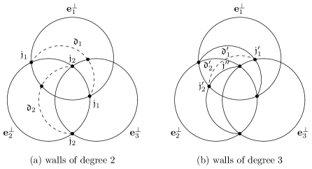
Figure 9: Construction of CSD of type $A_{3}$. A filled circle $\bullet$ represents a perpendicular joint. A dashed arc represents an attached wall of a given degree.

At degree $1$, there are three incoming walls $\mathbf{w}_{e_{i}}$ ($i=1,2,3$) as the initial input. Correspondingly, we have three circles representing their supports $\mathbf{e}_{i}^{\perp}$. Note that the inside and the outside of each circle $\mathbf{e}_{i}^{\perp}$ corresponds to the half spaces

$$\mathcal{H}_{i}^{>0}:=\{z\in M_{\mathbb{R}}\mid\langle e_{i},z\rangle>0\},\quad\mathcal{H}_{i}^{<0}:=\{z\in M_{\mathbb{R}}\mid\langle e_{i},z\rangle<0\},$$ (0.5.48)

respectively.

Now, we construct walls of degree $2$. We have two perpendicular joints $\mathfrak{j}_{1}=\mathbf{e}_{1}^{\perp}\cap\mathbf{e}_{2}^{\perp}=\mathbb{R}\mathbf{e}_{3}$, $\mathfrak{j}_{2}=\mathbf{e}_{2}^{\perp}\cap\mathbf{e}_{3}^{\perp}=\mathbb{R}\mathbf{e}_{1}$ to take care of, and the other joint $\mathfrak{j}_{3}=\mathbf{e}_{1}^{\perp}\cap\mathbf{e}_{3}^{\perp}=\mathbb{R}\mathbf{e}_{2}$ is parallel. Note that (only) these joints intersect the unit circle $S^{2}$ twice in $M_{\mathbb{R}}$. Therefore, there are two points representing each joint in the figure. First, consider the joint $\mathfrak{j}_{1}$. Since $\{\mathbf{e}_{2},\mathbf{e}_{1}\}=1$, the attached wall is

$$\mathbf{w}_{1}=(\mathfrak{d}_{1},\Psi[(1,1,0)])_{(1,1,0)},$$ (0.5.49)

$$\mathfrak{d}_{1}:=\sigma(\mathfrak{j}_{1},-p^{*}((1,1,0)))=\sigma((0,0,1),(0,0,-1),(1,-1,-1)).$$ (0.5.50)

where we note that $-p^{*}(\mathbf{n})=-B\mathbf{n}$. Since $\mathfrak{d}_{1}$ is in the “fourth quadrant”, it is inside the circle $\mathbf{e}_{1}^{\perp}$ and outside the circle $\mathbf{e}_{2}^{\perp}$ except for the boundary. It is depicted in the dashed arc in Figure 9 (a). Similarly, for the joint $\mathfrak{j}_{2}$, we have $\{\mathbf{e}_{3},\mathbf{e}_{2}\}=1$, and the attached wall is

$$\mathbf{w}_{1}=(\mathfrak{d}_{2},\Psi[(0,1,1)])_{(0,1,1)},$$ (0.5.51)

$$\mathfrak{d}_{2}:=\sigma(\mathfrak{j}_{2},-p^{*}((0,1,1)))=\sigma((1,0,0),(-1,0,0),(1,1,-1)).$$ (0.5.52)

This finishes the degree 2 walls.

Next, we construct walls of degree $3$. All joints that appeared above are already consistent. Thus, we concentrate on the newly created perpendicular joints $\mathfrak{j}^{\prime}_{1}=\mathfrak{d}_{1}\cap\mathbf{e}_{3}^{\perp}=\mathbb{R}_{\geq 0}(1,-1,0)$ and $\mathfrak{j}^{\prime}_{2}=\mathfrak{d}_{2}\cap\mathbf{e}_{1}^{\perp}=\mathbb{R}_{\geq 0}(0,1,-1)$ in Figure 9 (b). First, consider the joint $\mathfrak{j}^{\prime}_{1}$. Since $\{\mathbf{e}_{3},(1,1,0)\}=1$, the attached wall is

$$\mathbf{w}^{\prime}_{1}=(\mathfrak{d}^{\prime}_{1},\Psi[(1,1,1)])_{(1,1,1)},$$ (0.5.53)

$$\mathfrak{d}^{\prime}_{1}:=\sigma(\mathfrak{j}^{\prime}_{1},-p^{*}((1,1,1)))=\sigma((1,-1,0),(1,0,-1)).$$ (0.5.54)

Similarly, for the joint $\mathfrak{j}^{\prime}_{2}$, we have $\{(0,1,1),\mathbf{e}_{1}\}=1$, and the attached wall is

$$\mathbf{w}^{\prime}_{2}=(\mathfrak{d}^{\prime}_{2},\Psi[(1,1,1)])_{(1,1,1)},$$ (0.5.55)

$$\mathfrak{d}^{\prime}_{2}:=\sigma(\mathfrak{j}^{\prime}_{2},-p^{*}((1,1,1)))=\sigma((0,1,-1),(1,0,-1)).$$ (0.5.56)

The supports $\mathfrak{d}^{\prime}_{1}$ and $\mathfrak{d}^{\prime}_{2}$ are in the same hyperplane $(1,1,1)^{\perp}$. Moreover, they satisfy

$$\mathfrak{j}^{\prime\prime}:=\mathfrak{d}^{\prime}_{1}\cap\mathfrak{d}^{\prime}_{2}=\mathbb{R}_{\geq 0}(1,0,-1),\quad\mathfrak{d}^{\prime}_{1}\cup\mathfrak{d}^{\prime}_{2}=\sigma(\mathfrak{j}^{\prime}_{1},\mathfrak{j}^{\prime}_{2}).$$ (0.5.57)

Thus, $\mathfrak{d}^{\prime}_{1}$ and $\mathfrak{d}^{\prime}_{2}$ “shake hands” at $\mathfrak{j}^{\prime\prime}$ to make a cone $\sigma(\mathfrak{j}^{\prime}_{1},\mathfrak{j}^{\prime}_{2})$. (This shake-hands phenomenon is guaranteed to occur due to the consistency proved in Lemma 0.5.16.) Note that the algorithm does not request us to joint $\mathbf{w}^{\prime}_{1}$ and $\mathbf{w}^{\prime}_{2}$ into one wall. The cone $\sigma(\mathfrak{j}^{\prime}_{1},\mathfrak{j}^{\prime}_{2})$ is depicted in the dashed arc in Figure 9 (b). Moreover, we have $\sigma(\mathfrak{j}^{\prime}_{1},\mathfrak{j}^{\prime}_{2})\cap e_{2}^{\perp}=\mathfrak{j}^{\prime\prime}$, and $\{(1,1,1),\mathbf{e}_{2}\}=0$. Thus, the joint $\mathfrak{j}^{\prime\prime}$ is parallel (as it should be because $-p^{*}(1,1,1)\in\mathfrak{j}^{\prime\prime}$ by construction). Therefore, the construction completes. Observe that all normal vectors

$$\mathbf{e}_{1},\ \mathbf{e}_{2},\ \mathbf{e}_{3},\ (1,1,0),\ (0,1,1),\ (1,1,1)$$ (0.5.58)

exhaust the positive roots of the root system of type $A_{3}$.

Remark 0.5.19.

As this is of finite type, $\mathrm{Supp}(\mathfrak{D}_{\mathfrak{s}})$ in Figure 9 (b) coincides with the cluster complex of a cluster pattern of type $A_{3}$ [FZ03a]. We give more accounts in Section 0.6.6. It also coincides with the picture for the picture group of type $A_{3}$ in [IOTW, ITW, IT21], where the picture groups are defined based on the representation theory of (valued) quivers. Moreover, it also coincides with the mutation fan in [Rea14, Rea20b]. The same remark applies to the following examples (b) and (c). The appearance of the positive roots is explained by these theories. Nevertheless, the phenomenon that the pentagon relation reproduces root systems is remarkable and important, and it deserves to be investigated further from this new perspective.

(b). Type $B_{3}$. Consider the case

$$B=\begin{pmatrix}0&-1&0\\ 1&0&-1\\ 0&2&0\end{pmatrix},\quad\delta_{1}=\delta_{2}=1,\ \delta_{3}=2.$$ (0.5.59)

This is again of finite type. The construction is similar to Type $A_{3}$, but it involves joints of type $B_{2}$ in Section 0.2.2 as well. For example, to the perpendicular joint $\mathfrak{j}=\mathbf{e}_{2}^{\perp}\cap\mathbf{e}_{3}^{\perp}$, a wall $\mathbf{w}=(\mathfrak{d},\Psi[(0,1,1)]^{2})_{(0,1,1)}$ of degree 2 and a wall $\mathbf{w}^{\prime}=(\mathfrak{d}^{\prime},\Psi[(0,1,2)])_{(0,1,2)}$ of degree 3 are attached. The details are left to the reader as an exercise. The resulting CSD is depicted in Figure 10 (a). As observed therein, all supports of type $A_{3}$ in the case (a) appear again, and they are indicated by solid arcs. Newly added supports are indicated by dashed arcs, where they have normal vectors $(0,1,2)$, $(1,1,2)$, $(0,2,2)$ from longer to shorter arcs. All normal vectors

$$\mathbf{e}_{1},\ \mathbf{e}_{2},\ \mathbf{e}_{3},\ (1,1,0),\ (0,1,1),\ (1,1,1),\ (0,1,2),\ (1,1,2),\ (1,2,2)$$ (0.5.60)

exhaust the positive roots of the root system of type $B_{3}$ as expected.

Figure 10: Construction of CSDs of types $B_{3}$ and $C_{3}$. The solid arcs are the supports of type $A_{3}$, while the dashed arcs are the additional supports.

(c). Type $C_{3}$. Consider the case

$$B=\begin{pmatrix}0&-1&0\\ 1&0&-2\\ 0&1&0\end{pmatrix},\quad\delta_{1}=\delta_{2}=2,\ \delta_{3}=1.$$ (0.5.61)

This is again of finite type. The construction is similar to type $B_{3}$. However, it involves joints of type $C_{2}$, instead of type $B_{2}$, in Section 0.2.2. Note that this difference affects the configuration of attached walls. Also, for joints of type $A_{2}$ we apply the pentagon relation (0.1.56) with $c=1/2$. The resulting CSD is depicted in Figure 10 (b). Once again, all supports of type $A_{3}$ appear, and they are indicated by solid arcs. Newly added supports are indicated by dashed arcs, where they have normal vectors $(0,2,1)$, $(2,2,1)$, $(1,2,1)$ from longer to shorter arcs. All normal vectors

$$\mathbf{e}_{1},\ \mathbf{e}_{2},\ \mathbf{e}_{3},\ (1,1,0),\ (0,1,1),\ (1,1,1),\ (0,2,1),\ (1,2,1),\ (2,2,1)$$ (0.5.62)

exhaust the positive roots of the root system of type $C_{3}$. Moreover, we see in Figure 10 (a) and (b) that the CSDs of type $B_{3}$ and $C_{3}$ are topologically identical even though the process of the construction and the assignment of normal vectors are different. This agrees with the well-known duality between the cluster patterns of types $B_{r}$ and $C_{r}$ [FZ03a, FZ03b], and a more general result called the synchronicity on cluster patterns in [Nak21]; namely, any pair of cluster patterns with the initial exchange matrices $B$ and $-B^{T}$ share the same structure.

The examples (a)–(c) exhaust all rank 3 CSD of finite type with indecomposable $B$ up to mutation-equivalence in [FZ03a]. We will continue to study examples of rank 3 CSDs of infinite type in Section 0.6.7 after clarifying the chamber structure of CSDs.

Notes

The construction of a CSD in Construction 0.5.14 is a hybrid of the construction by [KS06, §10] and [GS11, §3] presented in [GHKK18, Appendix C.1] and the proof of the positivity in Theorem 0.5.2 in [GHKK18, Appendix C.3]. Algorithm 0.5.7, which is based on the pentagon relation in Proposition 0.1.14, substitutes for the perturbation trick and the change of lattice trick in [GHKK18, Appendix C.3]. Theorem 0.5.17 is implicit in [GHKK18, Appendix C.3].

0.6 Mutation invariance of CSDs

In this section we study the mutation invariance of CSDs, which is important to make the connection with cluster patterns.

0.6.1 Mutations of seed and CSD

Throughout the section, we fix $k\in\{1,\dots,r\}$ arbitrarily.

For any integer $a$, we define

$$[a]_{+}=\begin{cases}a&a\geq 0,\\ 0&a<0.\end{cases}$$ (0.6.1)

We have a useful formula

$$[a]_{+}-[-a]_{+}=a.$$ (0.6.2)

The following notion originates in [FG09, §1.2].

Definition 0.6.1 (Seed mutation).

Let $\mathfrak{s}=(e_{1},\dots,e_{r})$ be a seed for a given fixed data $\Gamma$, and let $k\in\{1,\dots,r\}$. We define a new seed $\mu_{k}(\mathfrak{s})=\mathfrak{s}^{\prime}=(e^{\prime}_{1},\dots,e^{\prime}_{r})$ for $\Gamma$ by

$$e^{\prime}_{i}=\begin{cases}-e_{k}&i=k,\\ e_{i}+[\{\delta_{k}e_{k},e_{i}\}]_{+}e_{k}&i\neq k,\end{cases}$$ (0.6.3)

which is called the mutation of $\mathfrak{s}$ in direction $k$.

Lemma 0.6.2.

The above $\mathfrak{s}^{\prime}$ is indeed a seed for $\Gamma$.

Proof.

The transformation (0.6.3) is written in the following matrix form,

$$(e^{\prime}_{1},\dots,e^{\prime}_{r})=(e_{1},\dots,e_{r})\begin{pmatrix}1&\\ &\ddots\\ [b_{k1}]_{+}&\cdots&-1&\cdots&[b_{kr}]_{+}\\ &&&\ddots\\ &&&&1\end{pmatrix},$$ (0.6.4)

where we recall that $b_{ki}=\{\delta_{k}e_{k},e_{i}\}$. The matrix is unimodular. Thus, $\mathfrak{s}^{\prime}$ is a basis of $N$. Also, the basis $(\delta_{1}e_{1},\dots,\delta_{r}e_{r})$ of $N^{\circ}$ transforms as

$$\delta_{i}e^{\prime}_{i}=\begin{cases}-\delta_{k}e_{k}&i=k,\\ \delta_{i}e_{i}+[\{e_{k},\delta_{i}e_{i}\}]_{+}\delta_{k}e_{k}&i\neq k.\end{cases}$$ (0.6.5)

Then, $(\delta_{1}e^{\prime}_{1},\dots,\delta_{r}e^{\prime}_{r})$ is a basis of $N^{\circ}$ by the same reason as above. ∎

Remark 0.6.3.

The mutation $\mu_{k}$ above is not involutive. Namely, $\mu_{k}(\mathfrak{s}^{\prime})\neq\mathfrak{s}$ in general. Indeed, the inverse of (0.6.3) is given by

$$e_{i}=\begin{cases}-e^{\prime}_{k}&i=k,\\ e^{\prime}_{i}+[\{-\delta_{k}e^{\prime}_{k},e^{\prime}_{i}\}]_{+}e^{\prime}_{k}&i\neq k.\end{cases}$$ (0.6.6)

Even though $\mu_{k}$ is not involutive, it is “involutive” in the following sense.

Lemma 0.6.4.

Let $\mathfrak{s}^{\prime\prime}=\mu_{k}(\mathfrak{s}^{\prime})$. Let $B_{\Gamma,\mathfrak{s}}$ be the matrix in (0.1.4). Then, we have $B_{\Gamma,\mathfrak{s}^{\prime\prime}}=B_{\Gamma,\mathfrak{s}}$. Thus, the associated groups $G_{\Gamma,\mathfrak{s}^{\prime\prime}}$ and $G_{\Gamma,\mathfrak{s}}$ are isomorphic.

Proof.

By (0.6.3), we have

$$e^{\prime\prime}_{i}=\begin{cases}e_{k}&i=k,\\ e_{i}+\{\delta_{k}e_{k},e_{i}\}e_{k}&i\neq k.\end{cases}$$ (0.6.7)

Then, it is easy to check the equality $B_{\Gamma,\mathfrak{s}^{\prime\prime}}=B_{\Gamma,\mathfrak{s}}$. The last claim follows from Proposition 0.1.23. ∎

Under the change of a basis of $N$ from $\mathfrak{s}$ to $\mathfrak{s}^{\prime}$, we have the following coordinate transformation.

Lemma 0.6.5.

For $n=\sum_{i=1}^{r}a_{i}e_{i}\in N$, let $n=\sum_{i=1}^{r}a^{\prime}_{i}e^{\prime}_{i}$. Then, we have

$$a^{\prime}_{i}=\begin{cases}\displaystyle-a_{k}+\sum_{j=1}^{r}[\{\delta_{k}e_{k},e_{j}\}]_{+}a_{j}&i=k,\\ a_{i}&i\neq k.\end{cases}$$ (0.6.8)

Proof.

Let $A$ be the matrix in (0.6.4). Then, $A^{2}=I$ holds. Thus, the column vector $\mathbf{a}=(a_{1},\dots,a_{r})$ transforms by $\mathbf{a}^{\prime}=A\mathbf{a}$. ∎

Below we use the principal $x$-representation in Section 0.4 and its variation. Thus, a wall is expressed by $\mathbf{w}=(\mathfrak{d},g)_{n}=[\mathfrak{d},f]_{n}$ interchangeably as specified in Definition 0.4.10. As a general rule to remember, we apply $p^{*}$ for $\mathfrak{d}$ and $n$, while we apply $\tilde{p}^{*}$ for wall functions $f$.

For any seed $\mathfrak{s}=(e_{1},\dots,e_{r})$ and $k\in\{1,\dots,r\}$, we define linear maps

$$\begin{matrix}S_{k}=S_{k,\mathfrak{s}}:&M_{\mathbb{R}}&\rightarrow&M_{\mathbb{R}}\\ &z&\mapsto&z+\langle\delta_{k}e_{k},z\rangle p^{*}(e_{k}),\end{matrix}$$ (0.6.9)

$$\begin{matrix}\tilde{S}_{k}=\tilde{S}_{k,\mathfrak{s}}:&\tilde{M}^{\circ}&\rightarrow&\tilde{M}^{\circ}\\ &\tilde{m}&\mapsto&\tilde{m}+\langle\delta_{k}e_{k},m\rangle\tilde{p}^{*}(e_{k}),\end{matrix}$$ (0.6.10)

$$\begin{matrix}S_{k}^{*}=S_{k,\mathfrak{s}}^{*}:&N&\rightarrow&N\\ &n&\mapsto&n+\{\delta_{k}e_{k},n\}e_{k},\end{matrix}$$ (0.6.11)

where we continue to use the notation $\tilde{m}=m+n^{\prime}$ ($m\in M^{\circ}$, $n^{\prime}\in N$). They are dual to each other in the following sense.

Lemma 0.6.6.

(a). The following equalities hold.

$$\langle S_{k}^{*}(n),S_{k}(z)\rangle =\langle n,z\rangle,$$ (0.6.12)

$$\langle S_{k}^{*}(n),\tilde{S}_{k}(\tilde{m})\rangle =\langle n,\tilde{m}\rangle=\langle n,m\rangle,$$ (0.6.13)

$$S_{k}(p^{*}(n)) =p^{*}(S_{k}^{*}(n)),$$ (0.6.14)

$$\tilde{S}_{k}(\tilde{p}^{*}(n)) =\tilde{p}^{*}(S_{k}^{*}(n)).$$ (0.6.15)

(b). We have

$$S_{k}^{*}(\delta_{i}e_{i})=\begin{cases}\delta_{k}e_{k}&i=k,\\ \delta_{i}e_{i}+\{e_{k},\delta_{i}e_{i}\}\delta_{k}e_{k}&i\neq k.\end{cases}$$ (0.6.16)

In particular, $S_{k}^{*}$ preserves $N^{\circ}$.

(c). For any $n\in N$, we have $n\in N^{\circ}$ if and only if $S^{*}_{k}(n)\in N^{\circ}$.

(d). Let $\delta(n)$ $(n\in N)$ be the normalization factor in Definition 0.1.18. Then, we have

$$\delta(S^{*}_{k}(n))=\delta(n).$$ (0.6.17)

Proof.

(a). We have

$$\begin{split}\langle S_{k}^{*}(n),S_{k}(z)\rangle&=\langle n+\{\delta_{k}e_{k},n\}e_{k},z+\langle\delta_{k}e_{k},z\rangle p^{*}(e_{k})\rangle\\ &=\langle n,z\rangle+\langle\delta_{k}e_{k},z\rangle\{n,e_{k}\}+\{\delta_{k}e_{k},n\}\langle e_{k},z\rangle\\ &=\langle n,z\rangle.\end{split}$$ (0.6.18)

$$\begin{split}\langle S_{k}^{*}(n),\tilde{S}_{k}(\tilde{m})\rangle&=\langle n+\{\delta_{k}e_{k},n\}e_{k},\tilde{m}+\langle\delta_{k}e_{k},m\rangle\tilde{p}^{*}(e_{k})\rangle\\ &=\langle n,\tilde{m}\rangle+\langle\delta_{k}e_{k},m\rangle\{n,e_{k}\}+\{\delta_{k}e_{k},n\}\langle e_{k},\tilde{m}\rangle\\ &=\langle n,\tilde{m}\rangle=\langle n,m\rangle.\end{split}$$ (0.6.19)

$$\begin{split}S_{k}(p^{*}(n))&=p^{*}(n)+\langle\delta_{k}e_{k},p^{*}(n)\rangle p^{*}(e_{k})\\ &=p^{*}(n+\{\delta_{k}e_{k},n\}e_{k})=p^{*}(S_{k}^{*}(n)).\end{split}$$ (0.6.20)

$$\begin{split}\tilde{S}_{k}(\tilde{p}^{*}(n))&=\tilde{p}^{*}(n)+\langle\delta_{k}e_{k},\tilde{p}^{*}(n)\rangle\tilde{p}^{*}(e_{k})\\ &=\tilde{p}^{*}(n+\{\delta_{k}e_{k},n\}e_{k})=\tilde{p}^{*}(S_{k}^{*}(n)).\end{split}$$ (0.6.21)

(b). This is clear by (0.6.11).

(c). The only-if-part follows from (b). The inverse of $S_{k}^{*}$ is given by

$$S_{k}^{*}{}^{-1}:N\rightarrow N,\quad n\mapsto n-\{\delta_{k}e_{k},n\}e_{k},$$ (0.6.22)

which also preserves $N^{\circ}$. Thus, the if-part also holds.

(d). This follows from (c). ∎

We define the half spaces of $M_{\mathbb{R}}$

$$\mathcal{H}_{k}^{+} =\mathcal{H}_{k,\mathfrak{s}}^{+}:=\{z\in M_{\mathbb{R}}\mid\langle e_{k},z\rangle\geq 0\},$$ (0.6.23)

$$\mathcal{H}_{k}^{-} =\mathcal{H}_{k,\mathfrak{s}}^{-}:=\{z\in M_{\mathbb{R}}\mid\langle e_{k},z\rangle\leq 0\}.$$ (0.6.24)

Then, we define a piecewise-linear transformation

$$\begin{matrix}T_{k}=T_{k,\mathfrak{s}}:&M_{\mathbb{R}}&\rightarrow&M_{\mathbb{R}}\\ &z&\mapsto&z+[\langle\delta_{k}e_{k},z\rangle]_{+}p^{*}(e_{k})=\begin{cases}S_{k}(z)&z\in\mathcal{H}_{k}^{+},\\ z&z\in\mathcal{H}_{k}^{-}.\end{cases}\end{matrix}$$ (0.6.25)

Definition 0.6.7 (Mutation of CSD).

Let $\mathfrak{D}_{\mathfrak{s}}$ be the CSD for a seed $\mathfrak{s}$ in Construction 0.5.14, thus, satisfying the properties in Proposition 0.5.18. Any wall of $\mathfrak{D}_{\mathfrak{s}}$ has the form

$$(\mathfrak{d},g)_{n}=\ (\mathfrak{d},\Psi[tn]^{s\delta(tn)})_{n}=[\mathfrak{d},(1+x^{\tilde{p}^{*}(tn)})^{s}]_{n}.$$ (0.6.26)

Then, we define

$$S_{k}(\mathfrak{d},g)_{n}:= \ (S_{k}(\mathfrak{d}),\Psi[S_{k}^{*}(tn)]^{s\delta(S_{k}^{*}(tn))})_{S_{k}^{*}(n)}$$ (0.6.27)

$$= \ [S_{k}(\mathfrak{d}),(1+x^{\tilde{S}_{k}(\tilde{p}^{*}(tn))})^{s}]_{S_{k}^{*}(n)}.$$ (0.6.28)

Note that for $n\in N^{+}$, $S_{k}^{*}(n)$ does not necessarily belong to $N^{+}$. However, we temporarily ignore this fact. For each $k\in\{1,\dots,r\}$, let $T_{k}(\mathfrak{D}_{\mathfrak{s}})$ be a collection of “walls” obtained from $\mathfrak{D}_{\mathfrak{s}}$ as follows:

(a). For each wall $\mathbf{w}=(\mathfrak{d},g)_{n}$ of $\mathfrak{D}_{\mathfrak{s}}$ other than $\mathbf{w}_{e_{k}}=(e_{k}^{\perp},\Psi[e_{k}]^{\delta_{k}})_{e_{k}}$, let $\mathfrak{d}_{+}=\mathfrak{d}\cap\mathcal{H}_{k}^{+}$, and $\mathfrak{d}_{-}=\mathfrak{d}\cap\mathcal{H}_{k}^{-}$. We split the wall $\mathbf{w}$ into two walls

$$\mathbf{w}_{+}=(\mathfrak{d}_{+},g)_{n},\quad\mathbf{w}_{-}=(\mathfrak{d}_{-},g)_{n},$$ (0.6.29)

where, if one of $\mathfrak{d}_{+}$ and $\mathfrak{d}_{-}$ is codimension more than $1$, we throw that part away. Then, we replace $\mathbf{w}_{+}$ with a new wall $S_{k}(\mathbf{w}_{+})$ in (0.6.27), while we leave $\mathbf{w}_{-}$ as it is.

(b). Replace $\mathbf{w}_{e_{k}}$ with $\mathbf{w}_{e^{\prime}_{k}}=(e^{\prime}_{k}{}^{\perp},\Psi[e^{\prime}_{k}]^{\delta_{k}})_{e^{\prime}_{k}}$. (Clearly, $e^{\prime}_{k}=-e_{k}\not\in N^{+}$.)

We call $T_{k}(\mathfrak{D}_{\mathfrak{s}})$ the mutation of $\mathfrak{D}_{\mathfrak{s}}$ in direction $k$.

By construction, we have

$$\mathrm{Supp}(T_{k}(\mathfrak{D}_{\mathfrak{s}}))=T_{k}(\mathrm{Supp}(\mathfrak{D}_{\mathfrak{s}})).$$ (0.6.30)

Let $n=\sum_{i=1}^{r}a_{i}e_{i}\in N_{\mathfrak{s}}^{+}$ be the normal vector of any wall in $\mathfrak{D}_{\mathfrak{s}}$. Then, by Lemma 0.6.6, the normal vector $n^{\prime}$ of the corresponding wall in $T_{k}(\mathfrak{D}_{\mathfrak{s}})$ defined above is given by

$$n^{\prime}=\sum_{i=1}^{r}b_{i}e_{i}=\begin{cases}-e_{k}&n=e_{k}\\ n+\{\delta_{k}e_{k},n\}e_{k}.&\text{$n$ is the normal vector of $\mathfrak{d}_{+}$},\\ n&\text{$n$ is the normal vector of $\mathfrak{d}_{-}$}.\end{cases}$$ (0.6.31)

Lemma 0.6.8.

Let $n^{\prime}$ be as above. Then, under the change of the coordinate transformation $n^{\prime}=\sum_{i=1}^{r}b_{i}e_{i}=\sum_{i=1}^{r}b^{\prime}_{i}e^{\prime}_{i}$, we have $b^{\prime}_{i}=a_{i}$ for $i\neq k$, while

$$b^{\prime}_{k}=\begin{cases}1&n=e_{k},\\ \displaystyle-a_{k}+\sum_{j=1}^{r}[\mp\{\delta_{k}e_{k},e_{j}\}]_{+}a_{j}&\text{$n$ is the normal vector of $\mathfrak{d}_{\pm}$}.\end{cases}$$ (0.6.32)

Proof.

This follows from (0.6.31) and Lemma 0.6.5, where we use (0.6.2) for the second case. ∎

The goal of this section to prove the following theorem, which is the second fundamental result on cluster scattering diagrams.

Theorem 0.6.9 (Mutation invariance of CSD [GHKK18, Theorem 1.24]).

The collection of walls $T_{k}(\mathfrak{D}_{\mathfrak{s}})$ is a consistent scattering diagram for the seed $\mathfrak{s}^{\prime}=\mu_{k}(\mathfrak{s})$. Moreover, $T_{k}(\mathfrak{D}_{\mathfrak{s}})$ is equivalent to a CSD $\mathfrak{D}_{\mathfrak{s}^{\prime}}$ for $\mathfrak{s}^{\prime}$.

We see in (0.6.32) that $b^{\prime}_{k}<0$ may occur. Therefore, for $T_{k}(\mathfrak{D}_{\mathfrak{s}})$ to be a scattering diagram for $\mathfrak{s}^{\prime}$, $g_{z}(\mathfrak{D}_{\mathfrak{s}})=\mathrm{id}$ should hold if $z$ is on a wall of $\mathfrak{D}_{\mathfrak{s}}$ such that $b^{\prime}_{k}<0$. This property is nontrivial, and so far we have no direct proof. (In the rank 2 case, however, we can directly prove it. See Example 0.6.22.) Below we follow the strategy by [GHKK18] to avoid this difficulty. The main idea of [GHKK18] is that we temporarily extend the notion of scattering diagrams by accepting the walls with $b^{\prime}_{k}<0$, then prove the uniqueness property of a CSD $\mathfrak{D}_{\mathfrak{s}^{\prime}}$ up to equivalence among such extended scattering diagrams.

0.6.2 Extended structure group

As mentioned above, following the strategy by [GHKK18], we temporarily loosen the condition $n\in N_{\mathrm{pr}}^{+}$ for the normal vector $n$ of a wall. We define

$$\overline{N}^{+}=\overline{N}_{k,\mathfrak{s}}^{+}:=\biggl{\{}\sum_{i=1}^{r}a_{i}e_{i}\mid a_{i}\in\mathbb{Z}_{\geq 0}\text{\ for $i\neq k$},\ a_{k}\in\mathbb{Z},\ \sum_{\scriptstyle i=1\atop\scriptstyle i\neq k}^{n}a_{i}>0\biggr{\}}.$$ (0.6.33)

In other words, we allow negative coefficients of $e_{k}$ in $n$, while we exclude $n=je_{k}$ ($j\in\mathbb{Z}$). Let $\overline{N}_{\mathrm{pr}}^{+}$ be the set of all primitive elements in $\overline{N}^{+}$.

Lemma 0.6.10.

The following facts hold:

(a). $e_{k}\not\in\overline{N}_{\mathrm{pr}}^{+}$.

(b). For $n\in N_{\mathrm{pr}}^{+}$ with $n\neq e_{k}$, we have $n,S^{*}_{k}(n)\in\overline{N}_{\mathrm{pr}}^{+}$.

Proof.

The only nontrivial claim is that $S^{*}_{k}(n)$ is primitive in (b). If it is not, $S^{*}_{k}(n)=jn^{\prime}$ for some $j\in\mathbb{Z}_{>1}$ and $n^{\prime}\in N$. Then, applying $S_{k}^{*}{}^{-1}$ in (0.6.22), we see that $n=S_{k}^{*}{}^{-1}(jn^{\prime})=jS_{k}^{*}{}^{-1}(n^{\prime})$ is not primitive. ∎

We define a degree function

$$\begin{matrix}\overline{\deg}:&\overline{N}^{+}&\rightarrow&\mathbb{Z}_{>0}\\ &\displaystyle\sum_{i=1}^{r}a_{i}e_{i}&\mapsto&\displaystyle\sum_{\scriptstyle i=1\atop\scriptstyle i\neq k}^{r}a_{i}.\end{matrix}$$ (0.6.34)

Define an $\overline{N}^{+}$-graded Lie algebra $\overline{\mathfrak{g}}$,

$$\overline{\mathfrak{g}}=\bigoplus_{n\in\overline{N}^{+}}\mathfrak{g}_{n},$$ (0.6.35)

which is parallel to $\mathfrak{g}$ in (0.1.17). Then, we repeat the construction of $\widehat{g}$ and $G$ in Section 0.1, where $N^{+}$ and $\deg(n)$ therein are replaced with $\overline{N}^{+}$ and $\overline{\deg}(n)$. Note that the corresponding Lie algebras $\overline{\mathfrak{g}}^{\leq\ell}$ are still nilpotent. Therefore, the construction works, and we obtain the completion $\widehat{\overline{\mathfrak{g}}}$ and the corresponding exponential group $\overline{G}$. The reason to exclude $e_{k}$ from $\overline{N}^{+}$ is now clear, because it is incompatible with the completion of $\overline{\mathfrak{g}}$. We call $\overline{G}$ the extended structure group for $\mathfrak{D}_{\mathfrak{s}}$ and $k$.

This, however, is not yet enough for our purpose. Let $G(\Psi[e_{k}])$ be the group freely generated by $\Psi[e_{k}]$. Since $\Psi[e_{k}]\not\in\overline{G}$, the product of $\Psi[e_{k}]$ and elements of $\overline{G}$ is not defined in $\overline{G}$. Instead of further extending $\overline{G}$, we extend the algebra $\mathbbm{k}[[\tilde{P}]]$ so that both $G(\Psi[e_{k}])$ and $\overline{G}$ act faithfully on it.

First, we define a monoid $\overline{P}\subset\tilde{M}^{\circ}$ as follows:

• $\overline{P}=\overline{\sigma}\cap\tilde{M}^{\circ}$, where $\overline{\sigma}$ is a $2r$-dimensional (not strongly convex) cone in $\tilde{M}_{\mathbb{R}}$ such that $\overline{\sigma}\cap(-\overline{\sigma})=\mathbb{R}\tilde{p}^{*}(e_{k})$.

• $\tilde{p}^{*}(e_{i}),\cdots,\tilde{p}^{*}(e_{r})\in\overline{P}$.

We may take $\tilde{P}$ in Section 0.4.2 as a submonoid of $\overline{P}$ in the positive side of $\tilde{p}^{*}(e_{k})$. Let $\mathbbm{k}[\overline{P}]$ be the monoid ring of $\overline{P}$ over $\mathbbm{k}$. Then, the group of units of $\overline{P}$ is given by $\overline{P}^{\times}=\overline{P}\cap\mathbb{R}\tilde{p}^{*}(e_{k})$. Let $\overline{J}$ be the maximal ideal of $\mathbbm{k}[\overline{P}]$ generated by $\overline{P}\setminus\overline{P}^{\times}$, and let ${\mathbbm{k}[[\overline{P}]]}$ be the completion with respect to $\overline{J}$. Furthermore, we consider the localization $R_{k}:={\mathbbm{k}[[\overline{P}]]}_{f[e_{k}]}$ of ${\mathbbm{k}[[\overline{P}]]}$ by $f[e_{k}]=1+x^{\tilde{p}^{*}(e_{k})}$. Namely, any element $f\in R_{k}$ is written as

$$f=\sum_{\tilde{m}\in\overline{P}}b_{\tilde{m}}(1+x^{\tilde{p}^{*}(e_{k})})^{-a_{\tilde{m}}}x^{\tilde{m}}\quad(a_{\tilde{m}}\in\mathbb{Z}_{\geq 0},\ b_{\tilde{m}}\in\mathbbm{k}),$$ (0.6.36)

where in the infinite sum there are only finitely many $j\in\mathbb{Z}$ such that $b_{\tilde{m}+j\tilde{p}^{*}(e_{k})}\neq 0$ for each $\tilde{m}\in\overline{P}$. We define the action of $\Psi[n]\in\overline{G}$ ($n\in\overline{N}^{+}$) and $\Psi[e_{k}]\in G(\Psi[e_{k}])$ on $R_{k}$ in the usual way as

$$\begin{split}&\Psi[n](f)=\sum_{\tilde{m}\in\overline{P}}b_{\tilde{m}}(1+x^{\tilde{p}^{*}(e_{k})}(1+x^{\tilde{p}^{*}(n)})^{\langle n,\tilde{p}^{*}(e_{k})\rangle})^{-a_{\tilde{m}}}x^{\tilde{m}}(1+x^{\tilde{p}^{*}(n)})^{\langle n,m\rangle}\\ &\quad=\sum_{\tilde{m}\in\overline{P}}b_{\tilde{m}}(1+x^{\tilde{p}^{*}(e_{k})})^{-a_{\tilde{m}}}\biggl{(}1+x^{\tilde{p}^{*}(e_{k})}\frac{(1+x^{\tilde{p}^{*}(n)})^{\langle n,\tilde{p}^{*}(e_{k})\rangle}-1}{1+x^{\tilde{p}^{*}(e_{k})}}\biggr{)}^{-a_{\tilde{m}}}\\ &\qquad\qquad\quad\times x^{\tilde{m}}(1+x^{\tilde{p}^{*}(n)})^{\langle n,m\rangle},\end{split}$$ (0.6.37)

$$\Psi[e_{k}](f)=\sum_{\tilde{m}\in\overline{P}}b_{\tilde{m}}(1+x^{\tilde{p}^{*}(e_{k})})^{-a_{\tilde{m}}}x^{\tilde{m}}(1+x^{\tilde{p}^{*}(e_{k})})^{\langle e_{k},m\rangle}.$$ (0.6.38)

The right hand sides are in $R_{k}$. Moreover, the actions are faithful as Proposition 0.1.8. Thus, we have the following result.

Lemma 0.6.11.

Both groups $G(\Psi[e_{k}])$ and $\overline{G}$ act faithfully as automorphisms of $R_{k}$. In particular, the product of $\Psi[e_{k}]$ and $g\in\overline{G}$ is defined in $\mathrm{Aut}(R_{k})$.

The wall elements $\Psi[e_{k}]^{\pm 1}$ appear only for the consistency relation around a joint $\mathfrak{j}\in e_{k}^{\perp}$. Moreover, the consistency relation has the form

$$g_{1}\Psi[e_{k}]^{\pm\delta_{k}}g_{2}\Psi[e_{k}]^{\mp\delta_{k}}=\mathrm{id}\quad(g_{1},g_{2}\in\overline{G}_{\mathfrak{j}}),$$ (0.6.39)

where $G_{\mathfrak{j}}$ is the one in the following lemma. Then, the lemma tells that the consistency relation essentially reduces to the one in $\overline{G}$.

Lemma 0.6.12 ([GHKK18, Lemma C.8]).

Let $n\in\overline{N}_{\mathrm{pr}}^{+}$ and $\mathfrak{j}=e_{k}^{\perp}\cap n^{\perp}$. Let $N_{\mathfrak{j}}$ be the one in (0.5.31), and let $\overline{N}_{\mathfrak{j},\mathrm{pr}}^{+}:=N_{\mathfrak{j}}\cap\overline{N}_{\mathrm{pr}}^{+}$. Let $\overline{G}_{\mathfrak{j}}$ be the subgroup of $\overline{G}$ generated by the parallel subgroups $\overline{G}_{n}^{\parallel}$ $(n\in\overline{N}_{\mathfrak{j},\mathrm{pr}}^{+})$. Then, we have

$$\Psi[e_{k}]^{\delta_{k}}\overline{G}_{\mathfrak{j}}\Psi[e_{k}]^{-\delta_{k}}\subset\overline{G}_{\mathfrak{j}},\quad\mbox{if $\{e_{k},n\}\geq 0$},$$ (0.6.40)

$$\Psi[e_{k}]^{-\delta_{k}}\overline{G}_{\mathfrak{j}}\Psi[e_{k}]^{\delta_{k}}\subset\overline{G}_{\mathfrak{j}},\quad\mbox{if $\{e_{k},n\}\leq 0$}.$$ (0.6.41)

Proof.

This is clear if $\{e_{k},n\}=0$. Suppose that $\{e_{k},n\}\neq 0$. Then, we obtain the same formula in Proposition 0.1.24 (a) by working with the action on $R_{k}$. The claim immediately follows from it. ∎

For the seed $\mathfrak{s}^{\prime}=\mu_{k}(\mathfrak{s})=(e^{\prime}_{1},\dots,e^{\prime}_{r})$, we repeat the same construction as above. Then, despite the asymmetry of the mutation in Remark 0.6.3, the following result holds, where ^′ indicates the corresponding ones for $\mathfrak{s}^{\prime}$:

Lemma 0.6.13.

$$\overline{N}^{+}=\overline{N}^{\prime}{}^{+},\quad\overline{\mathfrak{g}}=\overline{\mathfrak{g}}^{\prime},\quad\overline{G}=\overline{G}^{\prime}.$$ (0.6.42)

Moreover, $\overline{P}$ serves as $\overline{P}^{\prime}$ for $\mathfrak{s}^{\prime}$ so that

$${\mathbbm{k}[[\overline{P}]]}={\mathbbm{k}[[\overline{P}^{\prime}]]},\quad R_{k}=R^{\prime}_{k}.$$ (0.6.43)

Proof.

For example, the equality $\overline{N}^{+}=\overline{N}^{\prime}{}^{+}$ follows from (0.6.3) and (0.6.33). The last equality in (0.6.43) follows from the identity

$$1+x^{\tilde{p}^{*}(e_{k})}=x^{-\tilde{p}^{*}(e^{\prime}_{k})}(1+x^{\tilde{p}^{*}(e^{\prime}_{k})}).$$ (0.6.44)

∎

0.6.3 Extended scattering diagrams

Definition 0.6.14 (Extended scattering diagram).

For a seed $\mathfrak{s}$ and $k\in\{1,\dots,r\}$, an extended scattering diagram $\overline{\mathfrak{D}}$ for $(\mathfrak{s},k)$ is a collection of walls satisfying the following properties:

• A wall is either $\mathbf{w}_{e_{k}}=(e_{k}^{\perp},\Psi[e_{k}]^{\delta_{k}})_{e_{k}}$, or $\mathbf{w}=(\mathfrak{d},g)_{n}$ with $n\in\overline{N}^{+}_{\mathrm{pr}}$, $\mathfrak{d}\subset n^{\perp}$, $g\in\overline{G}_{n}^{\parallel}$, where $\mathfrak{d}$ is a cone of codimension 1 as usual. (In particular, $n\neq e_{k}$.)

• It satisfies the finiteness condition with respect to $\overline{G}$ and $\overline{\deg}$ for walls other than $\mathbf{w}_{e_{k}}$.

• There is at most one $\mathbf{w}_{e_{k}}$.

Thanks to Lemma 0.6.11, for any admissible curve $\gamma$ in $\overline{\mathfrak{D}}$, the path-ordered product $\mathfrak{p}_{\gamma,\overline{\mathfrak{D}}}$ is defined in $\mathrm{Aut}(R_{k})$ in the same way as before. Thus, the equivalence and the consistency of extended scattering diagrams and other related notions are defined in the same way as before. (In particular, the consistency condition around a joint $\mathfrak{j}\subset e_{k}^{\perp}$ makes sense in $\overline{G}$ thanks to Lemma 0.6.12.)

Remark 0.6.15.

In [GHKK18] the distinguished wall $\mathbf{w}_{e_{k}}$ is excluded from walls, and called the slab.

Lemma 0.6.16.

(a). Let $\mathfrak{D}_{\mathfrak{s}}$ be the CSD constructed in Construction 0.5.14. Then, $\mathfrak{D}_{\mathfrak{s}}$ is a consistent extended scattering diagram for $(\mathfrak{s},k)$.

(b). For the same CSD $\mathfrak{D}_{\mathfrak{s}}$ as above, the mutation $T_{k}(\mathfrak{D}_{\mathfrak{s}})$ is an extended scattering diagram for $(\mathfrak{s}^{\prime},k)$, where $\mathfrak{s}^{\prime}=\mu_{k}(\mathfrak{s})$.

Proof.

(a). For any wall of $\mathfrak{D}_{\mathfrak{s}}$ other than $\mathbf{w}_{e_{k}}$, its normal vector $n\in N_{\mathrm{pr}}^{+}$ is not $e_{k}$ by Proposition 0.5.18. Thus, $n$ belongs to $n\in\overline{N}^{+}_{\mathrm{pr}}$ by Lemma 0.6.10 (b).

Next, we show that $\mathfrak{D}_{\mathfrak{s}}$ satisfies the finiteness condition with respect to $\overline{G}$. This is not trivial, and it is equivalent to the following claim:

Claim. For each $n\in N^{+}$ with $n-e_{k}\not\in N^{+}$, there are only finitely many $j\in\mathbb{Z}_{>0}$ such that $\Psi[n+je_{k}]^{s\delta(n+je_{k})}$ is a wall element of $\mathfrak{D}_{\mathfrak{s}}$.

Let us prove Claim by the induction on $\ell=\overline{\deg}(n)$. Let $\ell=1$, namely, $n=e_{i}$ ($i\neq k$). Then, by Construction 0.5.14, such walls are created only from the perpendicular joint $\mathfrak{j}\subset e_{k}^{\perp}\cap e_{i}^{\perp}$ with an anti-ordered product of $\Psi[e_{i}]^{\delta_{i}}$ and $\Psi[e_{k}]^{\delta_{k}}$. By Proposition 0.1.24 (b), $j$ is bounded as

$$j\leq|\{\delta_{k}e_{k},e_{i}\}|.$$ (0.6.45)

Suppose that Claim holds up to $\ell$. Let $\overline{\deg}(n)={\ell}+1$. Then, a wall element of the form $\Psi[n+je_{k}]^{s\delta(n+je_{k})}$ is created in the following two ways:

• It is created from a perpendicular joint $\mathfrak{j}\not\subset e_{k}^{\perp}$ with an anti-ordered product of $\Psi[n^{\prime}+j^{\prime}e_{k}]$’s with $\overline{\deg}(n^{\prime})\leq\ell$.

• It is created from a perpendicular joint $\mathfrak{j}\subset e_{k}^{\perp}\cap n^{\perp}$ with an anti-ordered product of $\Psi[e_{k}]$ and $\Psi[n+j^{\prime}e_{k}]$, where the latter is created in (a).

There are only finitely many such walls by the induction assumption and Proposition 0.1.24 (b). Thus, Claim holds for ${\ell}+1$. Therefore, $\mathfrak{D}_{\mathfrak{s}}$ is an extended scattering diagram for $(\mathfrak{s},k)$.

Finally, we show the consistency of $\mathfrak{D}_{\mathfrak{s}}$ as an extended scattering diagram for $(\mathfrak{s},k)$. Recall that any wall element $\Psi[n]^{s\delta(n)}$ of $\mathfrak{D}_{\mathfrak{s}}$ also acts on $R_{k}$. Thus, for any admissible loop $\gamma$, the consistency relation $\mathfrak{p}_{\gamma,\mathfrak{D}_{\mathfrak{s}}}=\mathrm{id}$ along $\gamma$ holds in $\mathrm{Aut}(R_{k})$, where the path-ordered product is defined in the limit with respect to $\deg$. Let us temporally write the path-ordered products along $\gamma$ defined in the limit with respect to $\deg$ and $\overline{\deg}$ as $\mathfrak{p}_{\gamma}$ and $\overline{\mathfrak{p}}_{\gamma}$, respectively. Then, it is enough to prove the equality

$$\mathfrak{p}_{\gamma}=\overline{\mathfrak{p}}_{\gamma}.$$ (0.6.46)

For any integer $\ell>0$, let $C_{\ell}$ be the largest $j$ for $n$ with $\overline{\deg}(n)=\ell$ in Claim above. Then, the following inequalities hold for any $n\in N^{+}$ (the first inequality is trivial):

$$\overline{\deg}(n)\leq\deg(n)\leq\overline{\deg}(n)+C_{\overline{\deg}(n)}.$$ (0.6.47)

Thus, the limit $\ell=\deg(n)\rightarrow\infty$ implies the limit $\overline{\ell}=\overline{\deg}(n)\rightarrow\infty$, and vice versa. Thus, we have the equality (0.6.46). Therefore, $\mathfrak{D}_{\mathfrak{s}}$ is consistent as an extended scattering diagram for $(\mathfrak{s},k)$.

(b). For any wall of $T_{k}(\mathfrak{D}_{\mathfrak{s}})$ other than $\mathbf{w}_{e_{k}}$, its normal vector $S^{*}_{k}(n)$ belongs to $\overline{N}^{+}_{\mathrm{pr}}$ by Lemma 0.6.10 (b). The finiteness condition with respect to $\overline{G}$ follows from the finiteness condition of $\mathfrak{D}_{\mathfrak{s}}$, because $\overline{\deg}(S_{k}^{*}(n))=\overline{\deg}(n)$. Thus, $T_{k}(\mathfrak{D}_{\mathfrak{s}})$ is an extended scattering diagram for $(\mathfrak{s}^{\prime},k)$. ∎

We will soon show that $T_{k}(\mathfrak{D}_{\mathfrak{s}})$ is also consistent as an extended scattering diagram for $(\mathfrak{s}^{\prime},k)$. We first prove the following uniqueness theorem, which is a key of the strategy by [GHKK18]. The claim is parallel to Theorem 0.3.10 (b), but it will be proved by a different argument.

Proposition 0.6.17 (Cf. [GHKK18, Theorem 1.28]).

Let $\mathrm{In}_{\mathfrak{s}}$ be the one in (0.3.55). Then, any consistent extended scattering diagram $\overline{\mathfrak{D}}$ for $(\mathfrak{s},k)$ with

$$\overline{\mathfrak{D}}_{\mathrm{in}}=\mathrm{In}_{\mathfrak{s}}$$ (0.6.48)

is equivalent to a CSD $\mathfrak{D}_{\mathfrak{s}}$ as an extended scattering diagram.

Proof.

Any CSD $\mathfrak{D}_{\mathfrak{s}}$ satisfies the condition (0.6.48) by Lemma 0.6.16 and Definition 0.3.11. Thus, we prove the following more general claim.

Claim. Two consistent extended scattering diagrams $\overline{\mathfrak{D}}$, $\overline{\mathfrak{D}}^{\prime}$ satisfying the condition (0.6.48) are equivalent.

Suppose that both $\overline{\mathfrak{D}}$ and $\overline{\mathfrak{D}}^{\prime}$ satisfy the condition (0.6.48). Let $\overline{\mathfrak{C}}=\overline{\mathfrak{D}}^{\prime}-\overline{\mathfrak{D}}.$ be an extended scattering diagram defined in the same way as in the proof of Lemma 0.5.16. Namely, take all walls of $\overline{\mathfrak{D}}$, invert all wall elements, add all walls of $\overline{\mathfrak{D}}^{\prime}$, and eliminate all incoming walls because they cancel each other. Then, we have the following properties:

• $\overline{\mathfrak{D}}\sqcup\overline{\mathfrak{C}}$ and $\overline{\mathfrak{D}}^{\prime}$ are equivalent.

• All walls of $\overline{\mathfrak{C}}$ are outgoing.

• All walls of $\overline{\mathfrak{C}}$ have normal vectors other than $e_{k}$.

Now we prove that, for any $n\in\overline{N}_{\mathrm{pr}}^{+}$,

$$\pi_{\ell}(g_{z}(\overline{\mathfrak{C}}))=\mathrm{id}$$ (0.6.49)

holds for any general $z\in n^{\perp}$. We prove it by the induction on $\ell$. Let $\overline{\mathfrak{C}}_{\ell}$ be the reduction of $\overline{\mathfrak{C}}$ at $\ell$. We note the following:

• A parallel result to Lemma 0.3.6 holds for $\overline{G}$.

Figure 11: Admissible loop $\gamma$ in the proof of Proposition 0.6.17.

First, consider the case $\ell=1$. Let us fix $n\in(\overline{N}_{\mathrm{pr}}^{+})^{\leq 1}$, namely, $n=e_{i}+je_{k}$ ($i\neq k)$ for some $j\in\mathbb{Z}$. We consider the case $\{e_{k},n\}\geq 0$. (We work with all such $n$ simultaneously.) We first note that $p^{*}(n)\in\mathcal{H}_{k}^{+}$ and the claim (0.6.49) holds for $\ell=1$ in some neighborhood of $p^{*}(n)$ due to the absence of any incoming wall. Let $z_{1}$ and $z_{2}$ be any general points in $n^{\perp}$. We take an admissible loop $\gamma$ intersecting $n^{\perp}$ transversally only at $z_{1}$ and $z_{2}$. Let $\mathfrak{j}=n^{\perp}\cap e_{k}^{\perp}$. First, suppose that $\mathfrak{j}$ is not inside the loop $\gamma$. Then, every nontrivial element appearing in the products $\mathfrak{p}_{\gamma,\overline{\mathfrak{D}}_{1}}$ and $\mathfrak{p}_{\gamma,\overline{\mathfrak{D}}^{\prime}_{1}}$ belong to $\overline{G}$. Since $\overline{G}^{\leq 1}$ is abelian and $\overline{\mathfrak{D}}$ and $\overline{\mathfrak{D}}^{\prime}$ are consistent, we have

$$\pi_{1}(\mathfrak{p}_{\gamma,\overline{\mathfrak{C}}_{1}})=\pi_{1}(\mathfrak{p}_{\gamma,\overline{\mathfrak{D}}^{\prime}_{1}})\pi_{1}(\mathfrak{p}_{\gamma,\overline{\mathfrak{D}}_{1}}^{-1})=\mathrm{id}.$$ (0.6.50)

Then, by the decomposition of $\overline{G}^{\leq 1}$, which is parallel to Lemma 0.3.6, we have

$$\pi_{1}(g_{z_{1}}(\overline{\mathfrak{C}}))=\pi_{1}(g_{z_{2}}(\overline{\mathfrak{C}})).$$ (0.6.51)

It follows that $\pi_{1}(g_{z}(\overline{\mathfrak{C}}))=\mathrm{id}$ holds in $\mathrm{Int}(\mathcal{H}_{k}^{+})$, while $\pi_{1}(g_{z}(\overline{\mathfrak{C}}))$ is constant in $\mathrm{Int}(\mathcal{H}_{k}^{-})$.

Next, suppose that $\mathfrak{j}$ is inside the loop $\gamma$. One can choose $z_{1}\in n^{\perp}\cap\mathrm{Int}(\mathcal{H}_{k}^{+})$ and $z_{2}\in n^{\perp}\cap\mathrm{Int}(\mathcal{H}_{k}^{-})$ sufficiently close to each other so that $\gamma$ intersects only walls whose normal vectors are in $\overline{N}_{\mathfrak{j},\mathrm{pr}}^{+}$ of Lemma 0.6.12. See Figure 11. It follows from the result just obtained above that $\pi_{1}(g_{z_{1}}(\overline{\mathfrak{C}}))=\mathrm{id}$ on $n^{\perp}\cap\mathrm{Int}(\mathcal{H}_{k}^{+})$. Also, any other $n^{\prime}{}^{\perp}$ $(n^{\prime}\in\overline{N}_{\mathfrak{j},\mathrm{pr}}^{+})$ containing $\mathfrak{j}$ also satisfies $\{e_{k},n^{\prime}\}>0$. It follows that the factor $\Psi[e_{k}]^{\delta_{k}}C\Psi[e_{k}]^{-\delta_{k}}\in\overline{G}$ in $\mathfrak{p}_{\gamma,\overline{\mathfrak{D}}_{1}}$ and $\mathfrak{p}_{\gamma,\overline{\mathfrak{D}}^{\prime}_{1}}$ coming from the region $\mathcal{H}_{k}^{+}$ coincide modulo $\overline{G}^{>1}$. Thus, we have (0.6.50) again, and we obtain (0.6.51). Therefore, we conclude that (0.6.49) holds for $\ell=1$. The other case $\{e_{k},n\}\leq 0$ is similar by exchanging $\mathcal{H}_{k}^{+}$ and $\mathcal{H}_{k}^{-}$.

Next, suppose that (0.6.49) holds up to $\ell$ for any general $z\in M_{\mathbb{R}}$. Let us fix $n\in(\overline{N}_{\mathrm{pr}}^{+})^{\ell+1}$. We take an admissible loop $\gamma$ in a similar way to the above. Then, by the induction assumption, all factors of $\pi_{\ell+1}(\mathfrak{p}_{\gamma,\overline{\mathfrak{C}}_{\ell+1}})$ belongs to $\mathrm{Ker}\,\pi_{\ell+1,\ell}$, which is abelian as in Lemma 0.3.6. Then, by repeating the same argument as $\ell=1$, we have

$$\pi_{\ell+1}(\mathfrak{p}_{\gamma,\overline{\mathfrak{C}}_{\ell+1}})=\pi_{\ell+1}(\mathfrak{p}_{\gamma,\overline{\mathfrak{D}}^{\prime}_{\ell+1}})\pi_{\ell+1}(\mathfrak{p}_{\gamma,\overline{\mathfrak{D}}_{\ell+1}}^{-1})=\mathrm{id}.$$ (0.6.52)

Then, again by the decomposition of $\mathrm{Ker}\,\pi_{\ell+1,\ell}$, which is parallel to Lemma 0.3.6, we conclude that (0.6.49) holds for $\ell+1$. ∎

0.6.4 Proof of mutation invariance of CSDs

Let us complete the proof of Theorem 0.6.9. We have already seen in Lemma 0.6.16 that $T_{k}(\mathfrak{D}_{\mathfrak{s}})$ is an extended scattering diagram for $(\mathfrak{s}^{\prime},k)$.

We first prove the consistency of $T_{k}(\mathfrak{D}_{\mathfrak{s}})$ as an extended scattering diagram for $(\mathfrak{s}^{\prime},k)$. Let us introduce the following algebra automorphism of $R_{k}=R^{\prime}_{k}$,

$$\begin{matrix}\tilde{S}_{k}=\tilde{S}_{k,\mathfrak{s}}:&R_{k}&\rightarrow&R_{k}\\ &x^{\tilde{m}}&\mapsto&x^{\tilde{S}_{k}(\tilde{m})}=x^{\tilde{m}+\langle\delta_{k}e_{k},m\rangle\tilde{p}^{*}(e_{k})}\quad(\tilde{m}\in\overline{P}),\\ &(1+x^{\tilde{p}^{*}(e_{k})})^{-1}&\mapsto&(1+x^{\tilde{p}^{*}(e_{k})})^{-1}.\end{matrix}$$ (0.6.53)

Lemma 0.6.18.

The following equalities hold as an algebra automorphism of $R_{k}$:

$$\Psi[S^{*}_{k}(n)]\circ\tilde{S}_{k} =\tilde{S}_{k}\circ\Psi[n]\quad(n\in{N}^{+}),$$ (0.6.54)

$$\Psi[e^{\prime}_{k}]^{\delta_{k}} =\tilde{S}_{k}\circ\Psi[e_{k}]^{-\delta_{k}}.$$ (0.6.55)

Proof.

Here, we consider the action only on $x^{\tilde{m}}$. We have

$$\begin{split}(\Psi[S^{*}_{k}(n)]\circ\tilde{S}_{k})(x^{\tilde{m}})&=\Psi[S^{*}_{k}(n)](x^{\tilde{S}_{k}(\tilde{m})})\\ &=x^{\tilde{S}_{k}(\tilde{m})}\tilde{S}_{k}(f[n])^{\langle S^{*}_{k}(n),{\tilde{S}_{k}(\tilde{m})}\rangle}\\ &=\tilde{S}_{k}(x^{\tilde{m}}f[n]^{\langle n,m\rangle})\\ &=(\tilde{S}_{k}\circ\Psi[n])(x^{\tilde{m}}),\end{split}$$ (0.6.56)

where we used Lemma 0.6.6 (a) and (d). Also, we have

$$\begin{split}\Psi[e^{\prime}_{k}]^{\delta_{k}}(x^{\tilde{m}})&=x^{\tilde{m}}(1+x^{\tilde{p}^{*}(e^{\prime}_{k})})^{\langle\delta_{k}e^{\prime}_{k},m\rangle}\\ &=x^{\tilde{m}}(1+x^{-\tilde{p}^{*}(e_{k})})^{-\langle\delta_{k}e_{k},m\rangle}\\ &=x^{\tilde{m}+\langle\delta_{k}e_{k},m\rangle\tilde{p}^{*}(e_{k})}(1+x^{\tilde{p}^{*}(e_{k})})^{-\langle\delta_{k}e_{k},m\rangle}\\ &=\tilde{S}_{k}(x^{\tilde{m}}(1+x^{\tilde{p}^{*}(e_{k})})^{-\langle\delta_{k}e_{k},m\rangle})\\ &=(\tilde{S}_{k}\circ\Psi[e_{k}]^{-\delta_{k}})(x^{\tilde{m}}).\end{split}$$ (0.6.57)

The action on $(1+x^{\tilde{p}^{*}(e_{k})})^{-1}$ is similar and easier. ∎

Lemma 0.6.19.

$T_{k}(\mathfrak{D}_{\mathfrak{s}})$ is a consistent extended scattering diagram for $(\mathfrak{s}^{\prime},k)$.

Figure 12: Admissible loop $\gamma$ in the proof of Lemma 0.6.19.

Proof.

It is enough to prove the consistency as an extended scattering diagram for $(\mathfrak{s}^{\prime},k)$. In view of Lemma 0.2.14, it is enough to show that $\mathfrak{p}_{\gamma,T_{k}(\mathfrak{D}_{\mathfrak{s}})}=\mathrm{id}$ for any admissible loop $\gamma$. If $\gamma$ is entirely in $\mathcal{H}_{k}^{-}$, the claim follows from the consistency of $\mathfrak{D}_{\mathfrak{s}}$ as an extended scattering diagram for $(\mathfrak{s},k)$ in Lemma 0.6.16 (a). If $\gamma$ is entirely in $\mathcal{H}_{k}^{+}$, the claim follows from the consistency of $\mathfrak{D}_{\mathfrak{s}}$ and (0.6.54). Therefore, it is enough to consider the case where $\gamma$ crosses the hyperplane $e_{k}^{\perp}$ as in Figure 12, where $z_{0}$ is the base point of $\gamma$. Then, from the consistency of $\mathfrak{D}_{\mathfrak{s}}$, we have

$$\mathfrak{p}_{\gamma,\mathfrak{D}_{\mathfrak{s}}}=g_{+}\circ\Psi[e_{k}]^{-\delta_{k}}\circ g_{-}\circ\Psi[e_{k}]^{\delta_{k}}=\mathrm{id},$$ (0.6.58)

where $g_{\pm}$ is the contribution from each half space $\mathcal{H}_{k}^{\pm}$. Then, by the definition of $T_{k}(\mathfrak{D}_{\mathfrak{s}})$ and Lemma 0.6.18,

$$\begin{split}\mathfrak{p}_{\gamma,T_{k}(\mathfrak{D}_{\mathfrak{s}})}&=(\tilde{S}_{k}\circ g_{+}\circ\tilde{S}_{k}^{-1})\circ\Psi[e^{\prime}_{k}]^{\delta_{k}}\circ g_{-}\circ\Psi[e^{\prime}_{k}]^{-\delta_{k}}\\ &=\tilde{S}_{k}\circ(g_{+}\circ\Psi[e_{k}]^{-\delta_{k}}\circ g_{-}\circ\Psi[e_{k}]^{\delta_{k}})\circ\tilde{S}_{k}^{-1}\\ &=\mathrm{id}.\end{split}$$ (0.6.59)

∎

Next we prove the following property.

Lemma 0.6.20.

$T_{k}(\mathfrak{D}_{\mathfrak{s}})$ is equivalent to an extended scattering diagram $\overline{\mathfrak{D}}$ for $(\mathfrak{s}^{\prime},k)$ with

$$\overline{\mathfrak{D}}_{\mathrm{in}}=\mathrm{In}_{\mathfrak{s}^{\prime}},$$ (0.6.60)

where $\mathfrak{s}^{\prime}=\mu_{k}(\mathfrak{s})$.

Proof.

Let us write $\mathbf{w}^{\prime}_{i}:=\mathbf{w}_{e^{\prime}_{i}}$ for simplicity. For the sake of convenience, we restate here what should be proved.

Claim. $T_{k}(\mathfrak{D}_{\mathfrak{s}})$ is equivalent to an extended scattering diagram $\overline{\mathfrak{D}}$ for $(\mathfrak{s}^{\prime},k)$ satisfying the following properties:

• $\overline{\mathfrak{D}}$ contains a unique wall $\mathbf{w}^{\prime}_{k}=(e^{\prime}_{k}{}^{\perp},\Psi[e^{\prime}_{k}]^{\delta_{k}})_{e^{\prime}_{k}}$.

• For any $i\neq k$, $\overline{\mathfrak{D}}$ contains a unique wall $\mathbf{w}^{\prime}_{i}=(e^{\prime}_{i}{}^{\perp},\Psi[e^{\prime}_{i}]^{\delta_{i}})_{e^{\prime}_{i}}$.

• All other walls in $\overline{\mathfrak{D}}$ are outgoing.

The property (i) holds for $T_{k}(\mathfrak{D}_{\mathfrak{s}})$ by the construction. So, let us consider the properties (ii) and (iii). We note that, by the construction of $T_{k}(\mathfrak{D}_{\mathfrak{s}})$ in Definition 0.6.7, a wall $S_{k}(\mathbf{w}_{+})$ is incoming if and only if $\mathbf{w}_{+}$ is incoming. Thus, any incoming wall in $T_{k}(\mathfrak{D}_{\mathfrak{s}})$ other than $\mathbf{w}^{\prime}_{k}$ only comes from $\mathbf{w}_{i,+}=((e_{i}{}^{\perp})_{+},\Psi[e_{i}]^{\delta_{i}})_{e_{i}}$ or $\mathbf{w}_{i,-}=((e_{i}{}^{\perp})_{-},\Psi[e_{i}]^{\delta_{i}})_{e_{i}}$ $(i\neq k)$. For each $i\neq k$, we consider three cases.

Case 1. $\{\delta_{k}e_{k},e_{i}\}>0$. We have $p^{*}(e_{i})\in\mathcal{H}_{k}^{+}$. Thus, $\mathbf{w}_{i,+}$ is an incoming wall. Also, $S_{k}^{*}(e_{i})=e_{i}+\{\delta_{k}e_{k},e_{i}\}e_{k}=e^{\prime}_{i}$. Therefore, we have an incoming wall in $T_{k}(\mathfrak{D}_{\mathfrak{s}})$,

$$S_{k}(\mathbf{w}_{i,+})=((e^{\prime}_{i}{}^{\perp})_{-},\Psi[e^{\prime}_{i}]^{\delta_{i}})_{e^{\prime}_{i}}=\mathbf{w}^{\prime}_{i,-},$$ (0.6.61)

where the sign $\pm$ of $(e^{\prime}_{i}{}^{\perp})_{\pm}$ is with respect to $e^{\prime}_{k}=-e_{k}$. Then, up to equivalence, it is extended to $\mathbf{w}^{\prime}_{i}$ by adding outgoing walls.

Case 2. $\{\delta_{k}e_{k},e_{i}\}<0$. We have $p^{*}(e_{i})\in\mathcal{H}_{k}^{-}$. Thus, $\mathbf{w}_{i,-}$ is an incoming wall. Also, $e_{i}=e^{\prime}_{i}$. Therefore, we have an incoming wall in $T_{k}(\mathfrak{D}_{\mathfrak{s}})$,

$$\mathbf{w}_{i,-}=((e^{\prime}_{i}{}^{\perp})_{+},\Psi[e^{\prime}_{i}]^{\delta_{i}})_{e^{\prime}_{i}}=\mathbf{w}^{\prime}_{i,+}.$$ (0.6.62)

Again, up to equivalence, it is extended to $\mathbf{w}^{\prime}_{i}$ by adding outgoing walls.

Case 3. $\{\delta_{k}e_{k},e_{i}\}=0$. We have $p^{*}(e_{i})\in\mathcal{H}_{k}^{+}\cap\mathcal{H}_{k}^{-}$. Thus, $\mathbf{w}_{i,+}$ and $\mathbf{w}_{i,-}$ are both incoming walls, where $p^{*}(e_{i})$ is at the boundary of both walls $\mathbf{w}_{i,\pm}$. Also, $S_{k}^{*}(e_{i})=e^{\prime}_{i}$. Therefore, we have incoming walls $\mathbf{w}_{i,+}=\mathbf{w}^{\prime}_{i,-}$ and $\mathbf{w}_{i,-}=\mathbf{w}^{\prime}_{i,+}$ in $T_{k}(\mathfrak{D}_{\mathfrak{s}})$. Then, joining them back again, we have $\mathbf{w}^{\prime}_{i}$.

It is clear that the resulting extended scattering diagram $\overline{\mathfrak{D}}$ satisfies all desired properties. ∎

By Lemmas 0.6.19 and 0.6.20, up to equivalence, $T_{k}(\mathfrak{D}_{\mathfrak{s}})$ satisfies the assumption of $\overline{\mathfrak{D}}$ in Proposition 0.6.17 (by replacing $\mathfrak{s}$ therein with $\mathfrak{s}^{\prime}$). Thus, we conclude that $T_{k}(\mathfrak{D}_{\mathfrak{s}})$ is equivalent to $\mathfrak{D}_{\mathfrak{s}^{\prime}}$ as an extended scattering diagram for $(\mathfrak{s}^{\prime},k)$. Moreover, since our choice of $\mathfrak{D}_{\mathfrak{s}}$ is with minimal support by Proposition 0.5.18, so is $T_{k}(\mathfrak{D}_{\mathfrak{s}})$. Thus, we have

$$\mathrm{Supp}(T_{k}(\mathfrak{D}_{\mathfrak{s}}))=\mathrm{Supp}(\mathfrak{D}_{\mathfrak{s}^{\prime}}).$$ (0.6.63)

This implies that $T_{k}(\mathfrak{D}_{\mathfrak{s}})$ is actually an ordinary scattering diagram for $\mathfrak{s}^{\prime}$, and that it is equivalent to $\mathfrak{D}_{\mathfrak{s}^{\prime}}$ as an ordinary scattering diagram for $\mathfrak{s}^{\prime}$. This completes the proof of Theorem 0.6.9.

0.6.5 Admissible region

In view of the remark after Theorem 0.6.9, we have the following corollary of Theorem 0.6.9.

Corollary 0.6.21.

Let $\mathfrak{D}_{\mathfrak{s}}$ be a CSD for $\mathfrak{s}$. Let $n=\sum_{i=1}^{r}a_{i}e_{i}\in N_{\mathrm{pr}}^{+}$ such that $n\neq e_{1},\dots,e_{r}$, and let $z$ be any general point in $n^{\perp}$. For each $k=1,\dots,r$, we define

$$b^{\prime}_{k}=\begin{cases}-a_{k}+\sum_{j=1}^{r}[-\{\delta_{k}e_{k},e_{j}\}]_{+}a_{j}&z\in\mathcal{H}_{k}^{+},\\ -a_{k}+\sum_{j=1}^{r}[\{\delta_{k}e_{k},e_{j}\}]_{+}a_{j}&z\in\mathcal{H}_{k}^{-}.\end{cases}$$ (0.6.64)

Then, we have

$$g_{z}(\mathfrak{D}_{\mathfrak{s}})\neq\mathrm{id}\quad\Longrightarrow\quad\text{$b^{\prime}_{k}\geq 0$ for any $k$.}$$ (0.6.65)

It is an interesting problem to give a direct proof of this property and also to extend it to other classes of consistent scattering diagrams.

Let us call the region of $z\in M_{\mathbb{R}}$ that satisfies the condition $b^{\prime}_{k}\geq 0$ for any $k$ the admissible region for a CSD $\mathfrak{D}_{\mathfrak{s}}$, where nontrivial outgoing walls are allowed.

Figure 13: Admissible region for a CSD of rank 2.

Example 0.6.22.

Let us explicitly write down the condition (0.6.65) for the rank 2 CSDs in Sections 0.2.2 and 0.3.5. For $\{e_{2},e_{1}\}=0$, no $n\neq e_{1},e_{2}$ is allowed. This agrees with the CSD of type $A_{1}\times A_{1}$ therein. For $\{e_{2},e_{1}\}=1$, the quantities in (0.6.64) are given as

$$b^{\prime}_{1}=\begin{cases}-a_{1}+\delta_{1}a_{2}&z\in\mathcal{H}_{1}^{+},\\ -a_{1}&z\in\mathcal{H}_{1}^{-}.\end{cases}\quad b^{\prime}_{2}=\begin{cases}-a_{2}&z\in\mathcal{H}_{2}^{+},\\ -a_{2}+\delta_{2}a_{1}&z\in\mathcal{H}_{2}^{-},\end{cases}$$ (0.6.66)

where $a_{1},a_{2}\neq 0$. Then, the condition $b^{\prime}_{k}\geq 0$ ($k=1,2$) is equivalent to the condition

$$z\in\mathcal{H}_{1}^{+}\cap\mathcal{H}_{2}^{-},\quad\frac{1}{\delta_{1}}\leq\frac{a_{2}}{a_{1}}\leq\delta_{2}.$$ (0.6.67)

The first condition is equivalent to that a wall is outgoing, and the second condition follows from the formula (0.1.75). Therefore, we directly verified the property (0.6.65) in the rank 2 case. Let $\mathbf{z}=(z_{1},z_{2})\in\mathbb{R}^{2}$ be the point corresponding to $z\in M_{\mathbb{R}}$. Then, by (0.2.12), we have

$$\delta_{1}^{-1}a_{1}z_{1}+\delta_{2}^{-1}a_{2}z_{2}=0.$$ (0.6.68)

Thus, the condition (0.6.67) is rewritten as

$$z_{1}\geq 0,\quad z_{2}\leq 0,\quad-\delta_{2}\leq\frac{z_{2}}{z_{1}}\leq-\frac{1}{\delta_{1}}.$$ (0.6.69)

The admissible region is depicted in Figure 13.

0.6.6 Chamber structure, $G$-fan, and cluster complex

There is an important consequence of the mutation invariance of CSDs.

Suppose that $\mathfrak{D}_{\mathfrak{s}}$ is a CSD with minimal support. We first give few remarks:

• By Lemma 0.2.18, the interior $\mathrm{Int}(\mathcal{C}^{+}_{\mathfrak{s}})$ of the positive orthant $\mathcal{C}^{+}_{\mathfrak{s}}$ is a chamber of $\mathrm{Supp}(\mathfrak{D}_{\mathfrak{s}})$, namely, it is a connected component of $M_{\mathbb{R}}\setminus\mathrm{Supp}(\mathfrak{D}_{\mathfrak{s}})$. Also, since $\mathrm{Int}(\mathcal{C}^{+}_{\mathfrak{s}})$ is an open set, its boundary belongs to $\mathrm{Supp}(\mathfrak{D}_{\mathfrak{s}})$.

• For $\mathfrak{s}^{\prime}=\mu_{k}(\mathfrak{s})$, we define a cone in $M_{\mathbb{R}}$ of full dimension by

  $$\mathcal{C}^{\mathfrak{s}}_{\mathfrak{s}^{\prime}}:=T_{k,\mathfrak{s}}^{-1}(\mathcal{C}^{+}_{\mathfrak{s}^{\prime}}).$$ (0.6.70)

  Since $\mathrm{Int}(\mathcal{C}^{+}_{\mathfrak{s}^{\prime}})$ is a chamber of $\mathrm{Supp}(\mathfrak{D}_{\mathfrak{s}^{\prime}})$, $\mathrm{Int}(\mathcal{C}^{\mathfrak{s}}_{\mathfrak{s}^{\prime}})$ is a chamber of $\mathrm{Supp}(\mathfrak{D}_{\mathfrak{s}})$ by (0.6.30). More explicitly, $\mathcal{C}^{\mathfrak{s}}_{\mathfrak{s}^{\prime}}$ is the cone defined by, for $i=k$,

  $$\langle e^{\prime}_{k},T_{k}(z)\rangle=\langle-e_{k},z+\langle\delta_{k}e_{k},z\rangle p^{*}(e_{k})\rangle=-\langle e_{k},z\rangle\geq 0,$$ (0.6.71)

  and, for $i\neq k$, by (0.6.71),

  $$\begin{split}\langle e^{\prime}_{i},T_{k}(z)\rangle&=\langle e_{i}+[\{\delta_{k}e_{k},e_{i}\}]_{+}e_{k},z+[\langle\delta_{k}e_{k},z\rangle]_{+}p^{*}(e_{k})\rangle\\ &=\langle e_{i},z\rangle+[\{\delta_{k}e_{k},e_{i}\}]_{+}\langle e_{k},z\rangle\geq 0.\end{split}$$ (0.6.72)

  Thus, the cone $\mathcal{C}^{\mathfrak{s}}_{\mathfrak{s}^{\prime}}$ is adjacent to $\mathcal{C}_{\mathfrak{s}}^{+}$ with a common boundary in $e_{k}^{\perp}$.

• Let $\sigma$ be a face of $\mathcal{C}^{\mathfrak{s}}_{\mathfrak{s}^{\prime}}$ of codimension 1 with the normal vector $n$. Let $z\in\sigma$ be general. Then, $g_{z}(\mathfrak{D}_{\mathfrak{s}})$ is obtained by the pull-back of $g_{T_{k}(z)}(\mathfrak{D}_{\mathfrak{s}^{\prime}})=\Psi[e^{\prime}_{i}]^{\delta_{i}}$ by $T_{k}$. Thus, we have

  $$g_{z}(\mathfrak{D}_{\mathfrak{s}})=\Psi[n]^{\delta(n)}.$$ (0.6.73)

  Moreover, $\delta(n)=\delta_{i}$ for some $i\in\{1,\dots,r\}$.

We repeat the above argument for a sequence of mutations of seeds.

Definition 0.6.23 ($G$-cone/$G$-chamber).

Suppose that $\mathfrak{D}_{\mathfrak{s}}$ is a CSD with minimal support. We consider any sequence of mutations of seeds

$$\mathfrak{s}=\mathfrak{s}_{0}\buildrel\mu_{k_{0}}\over{\mapsto}\mathfrak{s}_{1}\buildrel\mu_{k_{2}}\over{\mapsto}\cdots\buildrel\mu_{k_{i-1}}\over{\mapsto}\mathfrak{s}_{i}.$$ (0.6.74)

We define a cone in $M_{\mathbb{R}}$ by

$$\mathcal{C}^{\mathfrak{s}}_{\mathfrak{s}_{i}}:=(T_{k_{0},\mathfrak{s}_{0}}^{-1}\circ\cdots\circ T_{k_{i-1},\mathfrak{s}_{i-1}}^{-1})(\mathcal{C}^{+}_{\mathfrak{s}_{i}}).$$ (0.6.75)

As a special case $i=0$, we set $\mathcal{C}^{\mathfrak{s}}_{\mathfrak{s}}:=\mathcal{C}^{+}_{\mathfrak{s}}$. Then, $\mathrm{Int}(\mathcal{C}^{\mathfrak{s}}_{\mathfrak{s}_{i}})$ is a chamber of $\mathrm{Supp}(\mathfrak{D}_{\mathfrak{s}})$. We call $\mathcal{C}^{\mathfrak{s}}_{\mathfrak{s}_{i}}$ and $\mathrm{Int}(\mathcal{C}^{\mathfrak{s}}_{\mathfrak{s}_{i}})$ a $G$-cone and a $G$-chamber of $\mathfrak{D}_{\mathfrak{s}}$. (In [GHKK18], $\mathcal{C}^{\mathfrak{s}}_{\mathfrak{s}_{i}}$ is called a cluster chamber.)

Let $\mathbb{T}_{r}$ be the $r$-regular tree wth edges labelled by $1$, …, $r$ such that all edges emanating from each vertex $t$ of $\mathbb{T}_{r}$ have different labels. We abuse the notation $\mathbb{T}_{r}$ for the set of all vertices of $\mathbb{T}_{r}$. We fix the initial vertex $t_{0}\in\mathbb{T}_{r}$ arbitrarily. Then, we attach $\mathcal{C}^{+}_{\mathfrak{s}}$ to $t_{0}$. Also, we attach $\mathcal{C}^{\mathfrak{s}}_{\mathfrak{s}_{i}}$ in (0.6.75) to $t_{i}$, where $t_{0}$ and $t_{i}$ are sequentially connected with edges labelled by $k_{0}$, …, $k_{i-1}$. Thus, the $G$-cones of $\mathfrak{D}_{\mathfrak{s}}$ are parametrized by $\mathbb{T}_{r}$, though this parametrization is not necessarily one-to-one. Then, under the identification $M_{\mathbb{R}}\simeq\mathbb{R}^{r}$, $f_{i}\mapsto\mathbf{e}_{i}$, any $G$-cone $\mathcal{C}^{\mathfrak{s}}_{\mathfrak{s}_{i}}$ is identified with the cone $\sigma(G^{t_{0}}_{t_{i}})$ spanned by the column vectors (the $g$-vectors) of the $G$-matrix $G^{t_{0}}_{t_{i}}$ in [FZ07] for the corresponding cluster pattern. The collection of $G$-cones $\sigma(G^{t_{0}}_{t})$ ($t\in\mathbb{T}_{r}$) and their faces constitutes a fan $\Delta(\mathbf{G}^{t_{0}})$ (the $G$-fan). Moreover, as a simplicial complex, the $G$-fan $\Delta(\mathbf{G}^{t_{0}})$ is isomorphic to the cluster complex in [FZ03a]. See Part II for details.

By repeatedly applying the result (0.6.73), we have the following property.

Proposition 0.6.24.

Let $\sigma$ be a face of a $G$-cone $\mathcal{C}^{\mathfrak{s}}_{\mathfrak{s}_{i}}$ of codimension 1 with the normal vector $n\in N_{\mathrm{pr}}^{+}$. Then, for any general $z\in\sigma$, we have

$$g_{z}(\mathfrak{D}_{\mathfrak{s}})=\Psi[n]^{\delta(n)}.$$ (0.6.76)

Moreover, $\delta(n)=\delta_{i}$ for some $i\in\{1,\dots,r\}$.

The above result implies that, in Theorem 0.5.2, for the walls that are faces of $G$-cones, only $s=t=1$ occurs.

Example 0.6.25.

(a). Let $\mathfrak{D}_{\mathfrak{s}}$ be any CSD of finite type with rank 2 or 3 in Sections 0.2.2 and 0.3.5. Then, the $G$-cones fill up the entire ambient space $\mathbb{R}^{r}$. In other words, $\mathrm{Supp}(\mathfrak{D}_{\mathfrak{s}})$ is naturally identified with the $G$-fan $\Delta(\mathbf{G}^{t_{0}})$ of the corresponding cluster pattern. In particular, the property (0.6.76) holds for any wall of $\mathfrak{D}_{\mathfrak{s}}$.

(b). Let $\mathfrak{D}_{\mathfrak{s}}$ be the CSD of type $A_{1}^{(1)}$ in Section 0.3.5. Then, the $G$-cones fill up the set $\mathbb{R}^{2}\setminus\mathbb{R}_{>0}(1,-1)$. In other words, $\mathrm{Supp}(\mathfrak{D}_{\mathfrak{s}})\setminus\mathbb{R}_{>0}(1,-1)$ in $\mathbb{R}^{2}\setminus\mathbb{R}_{\geq 0}(1,-1)$ is naturally identified with the $G$-fan $\Delta(\mathbf{G}^{t_{0}})$ of the corresponding cluster pattern. In particular, the property (0.6.76) holds for any wall in $\mathrm{Supp}(\mathfrak{D}_{\mathfrak{s}})\setminus\mathbb{R}_{>0}(1,-1)$. On the other hand, the wall in (0.3.69) is unreachable by cluster mutations (i.e., mutations in the sense of cluster algebras). The $A_{2}^{(2)}$ case is similar. For the non-affine type of rank 2 in Section 0.3.5, replace $\mathbb{R}_{>0}(1,-1)$ with the Badlands $\sigma(\mathbf{v}_{+},\mathbf{v}_{-})\setminus\{0\}$ therein, which is also unreachable by cluster mutations.

0.6.7 Rank 3 examples: infinite type

Let us continue to give examples of rank 3 CSDs based on Construction 0.5.14. Here we consider the CSDs of infinite type, which are further separated into affine and non-affine types. We use the same convention in Section 0.5.4 to present rank 3 CSDs.

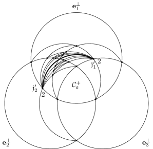
Figure 14: CSD of type $A_{2}^{(1)}$. The thick arc is unreachable by cluster mutations.

(a). Type $A_{2}^{(1)}$. As a prototypical example of affine type, we consider the following case

$$B=\begin{pmatrix}0&-1&-1\\ 1&0&-1\\ 1&1&0\end{pmatrix},\quad\delta_{1}=\delta_{2}=\delta_{3}=1.$$ (0.6.77)

As a new feature compared with the finite type, we have perpendicular joints of type $A_{1}^{(1)}$ in Section 0.3.5, which are given by $\mathfrak{j}^{\prime}_{1}\subset(1,1,0)^{\perp}\cap\mathbf{e}_{3}^{\perp}$ and $\mathfrak{j}^{\prime}_{2}\subset(0,1,1)^{\perp}\cap\mathbf{e}_{1}^{\perp}$ in Figure 14. Indeed, we have

$$\{\mathbf{e}_{3},(1,1,0)\}=\{(0,1,1),\mathbf{e}_{1}\}=2.$$ (0.6.78)

We put this number 2 in the figure in the position of incoming direction, so that outgoing walls appear in the opposite direction. These joints $\mathfrak{j}^{\prime}_{1}$ and $\mathfrak{j}^{\prime}_{2}$ are connected by walls with the common normal vector $(1,1,1)$, and their wall elements are given by $\Psi[(1,1,1)]^{2}$, $\Psi[(2,2,2)]$, $\Psi[(4,4,4)]^{1/2}$, …, based on the result the CSD of type $A_{1}^{(1)}$ in Section 0.3.5. The union of their supports is the cone $\sigma(\mathfrak{j}^{\prime}_{1},\mathfrak{j}^{\prime}_{2})$, and it is represented by a thick arc in Figure 14. It corresponds to the unreachable wall of type $A_{1}^{(1)}$ with the normal vector $(1,1)$ in Example 0.5.14 (b). Note that $\mathfrak{j}^{\prime}_{1}$ and $\mathfrak{j}^{\prime}_{2}$ are directly connected only by $\sigma(\mathfrak{j}^{\prime}_{1},\mathfrak{j}^{\prime}_{2})$, because a hyperplane containing $\mathfrak{j}^{\prime}_{1}$ and $\mathfrak{j}^{\prime}_{2}$ in $\mathbb{R}^{3}$ is unique. Consequently, $\mathfrak{j}^{\prime}_{1}$ and $\mathfrak{j}^{\prime}_{2}$ “alternately” create new walls, and they pile up as shown in the figure. We see that those walls with normal vectors

$$(2,1,1),\ (2,2,1),\ (3,2,2),\ (3,3,2),\ \dots$$ (0.6.79)

converge to the thick arc from above in the figure. Similarly, those walls with normal vectors

$$(1,1,2),\ (1,2,2),\ (2,2,3),\ (3,2,2),\ \dots$$ (0.6.80)

converges to the thick arc from below. This agrees with the well-known results on the cluster patterns of type $A_{2}^{(1)}$ by [FZ02] and [CI12]. We conclude that the $G$-cones fill up the region $\mathbb{R}^{3}\setminus(\sigma(\mathfrak{j}^{\prime}_{1},\mathfrak{j}^{\prime}_{2})\setminus\{0\})$. In other words, $\mathrm{Supp}(\mathfrak{D}_{\mathfrak{s}})\setminus(\sigma(\mathfrak{j}^{\prime}_{1},\mathfrak{j}^{\prime}_{2})\setminus\{0\})$ in $\mathbb{R}^{3}\setminus(\sigma(\mathfrak{j}^{\prime}_{1},\mathfrak{j}^{\prime}_{2})\setminus\{0\})$ is naturally identified with the $G$-fan $\Delta(\mathbf{G}^{t_{0}})$ of the corresponding cluster pattern. The walls in $\sigma(\mathfrak{j}^{\prime}_{1},\mathfrak{j}^{\prime}_{2})$ is unreachable by cluster mutations.

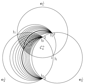
Figure 15: Example of rank 3 CSD of non-affine type. The close-up of the shaded region is given in Figure 16.

(b). Non-affine type. As a prototypical example of non-affine type, we consider the following case

$$B=\begin{pmatrix}0&-1&0\\ 1&0&-2\\ 0&2&0\end{pmatrix},\quad\delta_{1}=\delta_{2}=\delta_{3}=1.$$ (0.6.81)

The CSD has the remarkable fractal nature. This nature is simply originated in the fractal structure of the underlying $r$-regular tree $\mathbb{T}_{r}$ ($r\geq 3$) for the corresponding cluster complex, and it has been observed in some figures in the literature (e.g., [FG16, NC13]) for the so-called Markov quiver. This implies that it is impossible to draw a precise picture in principle. Thus, we change the strategy as follows:

• We set the goal to obtain a reasonably clear picture of the Badlands of rank 3.

• We abandon to faithfully follow Construction 0.5.14 by uniformly increasing the degree $\delta(n)$ of a newly attached wall element $\Psi[n]$. Rather, we do the mixture of Construction 0.5.14 and “cluster mutation approach”. Namely, having Construction 0.5.14 in mind, we increase the region of $G$-cones in the scattering diagram. Since the Badlands happens to be the complement of the $G$-fan in this example, the shape of the Badlands will gradually emerge by this procedure.

• While proceeding, we carefully choose added walls so that both local and global structures of the Badlands are better visible. (For example, we ignored some wall with degree 12, while we added a new wall of degree 245.)

• Due to the complexity we double-checked the result with a computer program for computing $c$-vectors of the cluster pattern. More specifically, we used SageMath 9.4 with Cluster Algebras package by D. Rupel and S. Stella.

The resulting CSD is depicted in Figures 15 and 16.

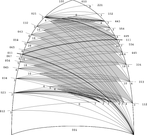
Figure 16: Uncompleted picture of the Badlands of rank 3. This is the close-up of the shaded region in Figure 15

Figures 15 gives the big picture of the CSD. Let $\mathcal{R}=\mathcal{H}_{1}^{>0}\cap\mathcal{H}_{2}^{>0}\cap\mathcal{H}_{3}^{<0}$, which corresponds to the shaded region in Figure 15. Outside the region $\mathcal{R}$, the structure of the CSD is clearly presented in the figure, where there are actually infinitely many walls converging to the unreachable walls attached to joints of type $A_{1}^{(1)}$ represented by two thick arcs. There is no more additional wall outside $\mathcal{R}$.

The close-up of the region $\mathcal{R}$ is given in Figure 16. This is where the Badlands and its fractal nature appear. Here are remarks and observations:

• A three-digit number such as 032 represents the normal vector (0,3,2) of a wall crossing the boundary of the region $\mathcal{R}$.

• A number such as 4 at a joint in $n_{1}^{\perp}\cap n_{2}^{\perp}$ represents $|\{n_{1},n_{2}\}|=4$. It is put in the position of incoming direction, so that outgoing walls appear in the opposite direction as in the previous case.

• A thick arc represents the supports of walls attached to a joint of type $A_{1}^{(1)}$ that is unreachable by cluster mutations. They consist of the “backbone” of the total shaded region (explained below). Six thick arcs are presented here, but in the limit $\ell\rightarrow\infty$ there will be infinitely many ones added in the top and bottom parts of the back-born. However, they will be so small and tightly aligned that they are not visible in this page size anyway.

• An unshaded triangle is already completed under the algorithm, and it is a $G$-cone. Meanwhile, a shaded triangle or quadrilateral is not completed yet. Thus, when the degree $\ell$ increases, the corners are sharpened and new corners appear. In other words, the total shaded region reduces, and the complexity of the boundary increases.

• By the above comments and the picture presented in Figure 16, it is already clear that in the limit $\ell\rightarrow\infty$ the total shaded region (in $\mathbb{R}^{3}$) converges to some connected closed domain, say $\mathcal{B}$. It is also characterized as the unreachable region by cluster mutations. The boundary of $\mathcal{B}$ is a fractal. Moreover, if the density conjecture on the Badlands of rank 2 in Section 0.3.5 holds, the set $\mathcal{B}$ is also densely filled with nontrivial walls. Thus, we call $\mathcal{B}$ the Badlands of this CSD.

Some other examples of rank 3 CSD of infinite type are found in [Mul16, Rea]. It seems that there are several patterns for non-affine infinite type CSDs even for the rank 3 case, and to classify them is an interesting problem.

Notes

Most results are taken from [GHKK18, §1.3, Appendix C.2] with added/modified proofs. In particular, the proof of Lemma 0.6.16 is significantly simplified from the one of [GHKK18, Theorem 1.28] by based on Construction 0.5.14 and Proposition 0.1.24 (b).

0.7 Broken lines and theta functions

In this section we introduce broken lines and theta functions for scattering diagrams. We prove the positivity of coefficients of theta functions for cluster scattering diagrams.

0.7.1 Broken lines and theta functions

In this section we again use the principal $x$-representation for wall elements. For notational simplicity, for any $\tilde{m}_{i}\in\tilde{M}^{\circ}=M^{\circ}\oplus N$, let $m_{i}$ denote the $M^{\circ}$-component of $\tilde{m}_{i}$. Namely, $\tilde{m}_{i}=m_{i}+n_{i}$ ($m_{i}\in M^{\circ}$, $n_{i}\in N$) for some $n_{i}$. We recall that $\langle n,\tilde{m}_{i}\rangle=\langle n,m_{i}\rangle$ holds for any $n\in N$ by (0.4.6).

Definition 0.7.1 (Broken line).

Let $\mathfrak{D}$ be any scattering diagram for a given initial seed $\mathfrak{s}$. Let $\tilde{m}_{0}\in\tilde{M}^{\circ}\setminus\{0\}$ and $Q\in M_{\mathbb{R}}\setminus\mathrm{Supp}(\mathfrak{D})$. A broken line for $\tilde{m}_{0}$ with endpoint $Q$ is a piecewise-linear curve $\gamma:(-\infty,0]\rightarrow M_{\mathbb{R}}\setminus\mathrm{Sing}(\mathfrak{D})$ satisfying the following properties:

• The endpoint $\gamma(0)$ is $Q$.

• The initial velocity $\gamma^{\prime}(t)$ in $t\rightarrow-\infty$ is $-m_{0}$.

• The curve $\gamma$ bends and change velocity only when it intersects walls of $\mathfrak{D}$. (It can cross walls also without bending and changing velocity.) Moreover, when $\gamma$ bends, it always crosses walls, not reflects at them.

More conditions follow below. Suppose that $\gamma$ bends $J\geq 0$ times. Let $t_{1}<t_{2}<\cdots<t_{J}<0$ be the points (“time”) of the parameter $t$ for $\gamma(t)$ when $\gamma$ bends. (It may cross multiple walls with a common normal vector at each time $t_{j}$.) We set $t_{0}=-\infty$ and $t_{J+1}=0$. Thus, $\gamma$ is linear and with constant velocity in each interval $I_{j}=(t_{j},t_{j+1})$ ($j=0,\dots,J$). As an extreme case, for $J=0$, the curve $\gamma$ is a half line ending at $Q$ with constant velocity $-m_{0}$. To each interval $I_{j}$, we attach a monomial $c_{j}x^{\tilde{m}_{j}}\in\mathbbm{k}[\tilde{M}^{\circ}]$ recursively as follows:

• To the initial interval $I_{0}$, the monomial $x^{\tilde{m}_{0}}$ is attached, where $\tilde{m}_{0}$ is the given data.

• For $j\geq 1$, let $\gamma_{j}$ be a segment of $\gamma$ for the interval $(t_{j}-\delta,t_{j}+\delta)$ with sufficiently small $\delta>0$ such that $\gamma_{j}$ crosses walls only at $t_{j}$. Then, $c_{j}x^{\tilde{m}_{j}}$ is a monomial in $\mathfrak{p}_{\gamma_{j},\mathfrak{D}}(c_{j-1}x^{\tilde{m}_{j-1}})$, where $\mathfrak{p}_{\gamma_{j},\mathfrak{D}}$ acts as the principal $x$-representation. See (0.7.5) for more explicit description.

Finally, the velocity of $\gamma$ in the interval $I_{j}$ is given as follows:

• The velocity $\gamma^{\prime}(t)$ in the interval $I_{j}$ is given by $-m_{j}$, where $c_{j}x^{\tilde{m}_{j}}$ is the attached monomial. This agrees with the conditions (2) and (4).

This completes the definition of a broken line. We then attach a monomial in $\mathbbm{k}[\tilde{M}^{\circ}]$ to each broken line $\gamma$ by

$$c_{\gamma}x^{\tilde{m}_{\gamma}}:=c_{J}x^{\tilde{m}_{J}}.$$ (0.7.1)

Several remarks are in order.

(a). At $t_{j}$, the velocity changes from $-m_{j}$ to $-m_{j+1}=-m_{j}-k_{j}p^{*}(n_{j})$, where $n_{j}$ is the common normal vector of the walls at $t_{j}$, and $k_{j}$ is some positive integer. Since $p^{*}(n_{j})\in n_{j}^{\perp}$, the broken line always crosses walls, not reflects nor stops at them as stated in the condition (3).

(b). In particular, we have $\tilde{m}_{j}=\tilde{m}_{0}+\sum_{i=1}^{r}a_{i}\tilde{p}^{*}(e_{i})$ $(a_{i}\in\mathbb{Z}_{\geq 0})$.

(c). For $\tilde{m}^{\prime}=\tilde{m}_{0}+\sum_{i=1}^{r}a_{i}\tilde{p}^{*}(e_{i})$, we define the degree $\deg_{\tilde{m}_{0}}(\tilde{m}^{\prime})$ by

$$\deg_{\tilde{m}_{0}}(\tilde{m}^{\prime}):=\sum_{i=1}^{r}a_{i}.$$ (0.7.2)

Then, by (a), we have

$$\deg_{\tilde{m}_{0}}(\tilde{m}_{0})=0<\deg_{\tilde{m}_{0}}(\tilde{m}_{1})<\cdots<\deg_{\tilde{m}_{0}}(\tilde{m}_{J})=\deg_{\tilde{m}_{0}}(\tilde{m}_{\gamma}).$$ (0.7.3)

(d). For the segment $\gamma_{j}$ in the condition (5), suppose that $\gamma_{j}$ crosses walls $[\mathfrak{d}_{\lambda},f_{{\lambda}}]_{n_{j}}$ $(\lambda\in\Lambda_{j}$) at $t_{j}$. Note that $\gamma^{\prime}=-m_{j-1}$ just before $\gamma$ crosses these walls. Then, the intersection signs in (0.2.6) are given by

$$\epsilon_{j}=\begin{cases}1&\langle n_{j},m_{j-1}\rangle>0,\\ -1&\langle n_{j},m_{j-1}\rangle<0.\\ \end{cases}$$ (0.7.4)

Thus, $\epsilon_{j}\langle n_{j},m_{j-1}\rangle=|\langle n_{j},m_{j-1}\rangle|$. Therefore, by Definition 0.2.6, we have

$$\mathfrak{p}_{\gamma_{j},\mathfrak{D}}(c_{j-1}x^{\tilde{m}_{j-1}})=c_{j-1}x^{\tilde{m}_{j-1}}\prod_{\lambda\in\Lambda_{j}}f_{{\lambda}}^{|\langle\delta(n_{j})n_{j},m_{j-1}\rangle|}.$$ (0.7.5)

It is crucial that there is no division by $f_{{\lambda}}$ in this expression for the forthcoming positivity of theta functions.

Definition 0.7.2 (General position).

We say that $Q\in M_{\mathbb{R}}\setminus\mathrm{Supp}(\mathfrak{D})$ is in general position if for each $\ell>0$ there is some neighborhood $U_{\ell}$ of $Q$ such that, for the reduction $\mathfrak{D}_{\ell}$, any broken line for $Q^{\prime}\in U_{\ell}$ converges to a broken line for $Q$ in the limit $Q^{\prime}\rightarrow Q$. (Namely, no broken line crosses $\mathrm{Sing}(\mathfrak{D}_{\ell})$ in the limit.)

Below we always and implicitly assume that $Q$ is in general position.

Definition 0.7.3 (Theta function).

Under the same assumption and notations in Definition 0.7.1, the theta function $\vartheta_{Q,\tilde{m}_{0}}$ for $\tilde{m}_{0}$ with endpoint $Q$ is defined by

$$\vartheta_{Q,\tilde{m}_{0}}:=\sum_{\gamma\in B(Q,\tilde{m}_{0})}c_{\gamma}x^{\tilde{m}_{\gamma}},$$ (0.7.6)

where $B(Q,\tilde{m}_{0})$ is the set of all broken lines for $\tilde{m}_{0}$ with endpoint $Q$. We also set

$$\vartheta_{Q,0}=1.$$ (0.7.7)

The function $\vartheta_{Q,\tilde{m}_{0}}$ only depends on the equivalence class of $\mathfrak{D}$, though the condition for $Q$ to be in general position depends on the choice of a representative of $\mathfrak{D}$.

Lemma 0.7.4 ([GHKK18, Proposition 3.4]).

For any scattering diagram $\mathfrak{D}$, we have

$$\vartheta_{Q,\tilde{m}_{0}}\in x^{\tilde{m}_{0}}\mathbbm{k}[[\tilde{P}]].$$ (0.7.8)

Proof.

By Remark (b), each term $c_{\gamma}x^{\tilde{m}_{\gamma}}$ belongs to $x^{\tilde{m}_{0}}\mathbbm{k}[[\tilde{P}]]$. Thus, it is enough to show that, for a given $\tilde{m}^{\prime}\in\tilde{m}_{0}+\tilde{P}$, there are only finitely many $\gamma$ such that $\tilde{m}_{\gamma}=\tilde{m}^{\prime}$. We note the following facts:

• By the constraint (0.7.3), such $\gamma$ bends at most $\deg_{\tilde{m}_{0}}(\tilde{m}^{\prime})$ times.

• The walls of $\mathfrak{D}$ that contribute to $\tilde{m}^{\prime}$ belongs to the reduction $\mathfrak{D}_{\ell}$ at $\ell=\deg_{\tilde{m}_{0}}(\tilde{m}^{\prime})$, which has only finitely many walls.

• At each bending there are only finitely many possibilities of bending.

Therefore, there are only finitely many possibilities of such $\gamma$. ∎

Proposition 0.7.5 ([GHKK18, Proposition 3.8]).

Let $\mathfrak{D}$ be any scattering diagram for a given seed $\mathfrak{s}$, and let $\mathcal{C}^{+}_{\mathfrak{s}}$ be the positive orthant in (0.2.40). For $\tilde{m}_{0}\in\tilde{M}^{\circ}$, suppose that $m_{0}\in\mathcal{C}^{+}_{\mathfrak{s}}\cap M^{\circ}$. Also, suppose that $Q\in\mathrm{Int}(\mathcal{C}^{+}_{\mathfrak{s}})$. Then, we have

$$\vartheta_{Q,\tilde{m}_{0}}=x^{\tilde{m}_{0}}.$$ (0.7.9)

Proof.

We may assume that $\tilde{m}_{0}\neq 0$. It is clear that $Q+\mathbb{R}_{\geq 0}m_{0}$ is a broken line for $\tilde{m}_{0}$ with end point $Q$, and it does not intersect any walls of $\mathfrak{D}_{\mathfrak{s}}$; therefore, the associated monomial is $x^{\tilde{m}_{0}}$. We claim that under the condition there is no broken line $\gamma$ with bending. Suppose that such $\gamma$ exists. We use the notation in Definition 0.7.1. For each break point $t_{j}$ therein, let $n_{j}\in N^{+}$ be a unique (not necessarily primitive) element such that $\gamma$ intersects walls in $n_{j}^{\perp}$ at $t_{j}$ and that the velocity of $\gamma$ is shifted by $-p^{*}(n_{j})$. Let $L_{j}$ be the segment of $\gamma$ for the interval $I_{j}$. Then, we claim the following:

$$L_{j}\subset H_{j}^{-}:=\biggl{\{}z\in M_{\mathbb{R}}\biggm{|}\biggl{\langle}\sum_{i=1}^{j}n_{i},z\biggr{\rangle}\leq 0\biggr{\}}\quad(j=1,\dots,J).$$ (0.7.10)

We show it by the induction on $j$. This is true for $j=1$, because the support of the wall crossed by $\gamma$ at $t_{1}$ is in $n_{1}^{\perp}$, and $\gamma$ is in $\mathcal{C}^{+}_{\mathfrak{s}}$ for $t\rightarrow-\infty$. Now suppose that (0.7.10) hold up to $j$. Then, we have $\langle\sum_{i=1}^{j}n_{i},\gamma(t_{j+1})\rangle\leq 0$. Also, $\langle n_{j+1},\gamma(t_{j+1})\rangle=0$. Thus, $\gamma(t_{j+1})\in H_{j+1}^{-}$. Moreover, the new velocity vector $\gamma^{\prime}_{j+1}=-m_{0}-\sum_{i=1}^{j+1}p^{*}(n_{i})$ satisfies the inequality

$$\begin{split}\biggl{\langle}\sum_{i=1}^{j+1}n_{i},\gamma^{\prime}_{j+1}\biggr{\rangle}&=\biggl{\langle}\sum_{i=1}^{j+1}n_{i},-m_{0}\biggr{\rangle}+\biggl{\{}\sum_{i=1}^{j+1}n_{i},\sum_{i=1}^{j+1}n_{i}\biggr{\}}\\ &=\biggl{\langle}\sum_{i=1}^{j+1}n_{i},-m_{0}\biggr{\rangle}\leq 0.\end{split}$$ (0.7.11)

Thus, the fact (0.7.10) holds for $j+1$. Since $\mathrm{Int}(\mathcal{C}^{+}_{\mathfrak{s}})\cap H_{j}^{-}=\emptyset$, $\gamma$ cannot reach $Q\in\mathrm{Int}(\mathcal{C}^{+}_{\mathfrak{s}})$. ∎

0.7.2 Transitivity on theta functions

Now we assume that $\mathfrak{D}$ is consistent.

Proposition 0.7.6 ([CPS, Lemma 4.9]).

Let $\mathfrak{D}$ be a consistent scattering diagram. Let $\tilde{m}_{0}\in\tilde{M}^{\circ}$ and $Q,\,Q^{\prime}\in M_{\mathbb{R}}\setminus\mathrm{Supp}(\mathfrak{D})$. Then, for any admissible curve $\gamma$ from $Q$ to $Q^{\prime}$, we have

$$\vartheta_{Q^{\prime},\tilde{m}_{0}}=\mathfrak{p}_{\gamma,\mathfrak{D}}(\vartheta_{Q,\tilde{m}_{0}}).$$ (0.7.12)

The rest of this subsection is devoted to prove this proposition. We may assume that $\tilde{m}_{0}\neq 0$.

Let $J$ be the maximal ideal of $\mathbbm{k}[[\tilde{P}]]$ generated by $\tilde{P}\setminus\{0\}$.

Lemma 0.7.7 ([CPS, Lemma 4.7]).

Let $\mathfrak{D}_{\ell}$ be the reduction of $\mathfrak{D}$ at $\ell$. Suppose that $Q$ and $Q^{\prime}$ are in the same chamber of $\mathrm{Supp}(\mathfrak{D}_{\ell})$. Then, we have the equality

$$\vartheta_{Q,\tilde{m}_{0}}\equiv\vartheta_{Q^{\prime},\tilde{m}_{0}}\mod x^{\tilde{m}_{0}}J^{\ell+1}.$$ (0.7.13)

Proof.

Since we consider $\vartheta_{Q,\tilde{m}_{0}}$ only modulo $x^{\tilde{m}_{0}}J^{\ell+1}$, one can replace $\mathfrak{D}$ with $\mathfrak{D}_{\ell}$ to calculate $\vartheta_{Q,\tilde{m}_{0}}$. First, suppose that $Q$ and $Q^{\prime}$ are connected by a curve $\beta$ in the same chamber such that any point on $\beta$ is in general position for $\mathfrak{D}_{\ell}$. Then, each broken line with endpoint $Q$ continuously deformed to a broken line with endpoint $Q^{\prime}$. Therefore, the theta function is unchanged.

Suppose that there is no such curve between $Q$ and $Q^{\prime}$. Let us consider the special case where $Q$ and $Q^{\prime}$ are connected by a curve $\beta$ in the same chamber such that there is a unique point $Q_{0}$ on $\beta$ that is not in general position. (The general case reduces to this case.) Then, there is at least one broken line $\gamma$ with endpoint $Q$ such that, in the limit $Q\rightarrow Q_{0}$, the broken line intersects with some boundary $\partial\mathfrak{d}$ or joint $\mathfrak{j}=\mathfrak{d}_{1}\cap\mathfrak{d}_{2}$ of $\mathfrak{D}_{\ell}$.

Figure 17: Broken lines in the proof of Lemma 0.7.7.

First, let us consider the case $\mathfrak{j}$. See Figure 17 (a). Suppose that $\gamma$ crosses the walls that contain the joint $\mathfrak{j}$ with the incoming attached monomial $c_{\mathrm{in}}x^{\tilde{m}_{\mathrm{in}}}$ and the outgoing attached monomial $c_{\mathrm{out}}x^{\tilde{m}_{\mathrm{out}}}$. There may be several broken lines $\gamma_{1}=\gamma$, …, $\gamma_{p}$ with endpoint $Q$ such that their bending patterns differ from $\gamma$ only inside these walls. They have the common incoming attached monomial $c_{\mathrm{in}}x^{\tilde{m}_{\mathrm{in}}}$ and the common exponent $\tilde{m}_{\mathrm{out}}$ for the outgoing attached monomials. Then, all these broken lines have a common limit for $Q\rightarrow Q_{0}$. Let $\gamma_{A}$ be the half of a small loop around $\mathfrak{j}$, which is on the same side of $\mathfrak{j}$ with $\gamma_{i}$’s as in Figure 17 (a). Then, the sum of the outgoing attached monomials for $\gamma_{1}$, …, $\gamma_{p}$ is exactly the terms of the monomials in $\mathfrak{p}_{\gamma_{A},\mathfrak{D}_{\ell}}(c_{\mathrm{in}}x^{\tilde{m}_{\mathrm{in}}})$ with exponents $x^{\tilde{m}_{\mathrm{out}}}$. We repeat the same argument to the opposite side of $\mathfrak{j}$ with the opposite half $\gamma_{B}$ of the small loop around $\mathfrak{j}$. Then, by the consistency of $\mathfrak{D}$, we have

$$\mathfrak{p}_{\gamma_{A},\mathfrak{D}_{\ell}}(c_{\mathrm{in}}x^{\tilde{m}_{\mathrm{in}}})\equiv\mathfrak{p}_{\gamma_{B},\mathfrak{D}_{\ell}}(c_{\mathrm{in}}x^{\tilde{m}_{\mathrm{in}}})\mod x^{\tilde{m}_{0}}J^{\ell+1}.$$ (0.7.14)

Thus, passing through $Q_{0}$ does not change $\vartheta_{Q,\tilde{m}_{0}}$ modulo $x^{\tilde{m}_{0}}J^{\ell+1}$. Therefore, we obtain the equality (0.7.13).

Next, we consider the remaining case $\partial\mathfrak{d}$. See Figure 17 (b). We may concentrate on a face $\mathfrak{c}$ of $\mathfrak{d}$ of codimension 2 such that $\mathfrak{c}$ is not a joint. Then, $\mathfrak{c}$ is contained in some walls of $\mathfrak{D}_{\ell}$ with the common normal vector $n$. In this case, for each broken line for $Q$, there is a unique broken line for $Q^{\prime}$ with the same attached incoming and outgoing monomial modulo $x^{\tilde{m}_{0}}J^{\ell+1}$, thanks to the consistency of $\mathfrak{D}$. Thus, passing through $Q_{0}$ does not change $\vartheta_{Q,\tilde{m}_{0}}$ modulo $x^{\tilde{m}_{0}}J^{\ell+1}$. ∎

Lemma 0.7.8 ([CPS, Lemma 4.8]).

Suppose that $Q$ and $Q^{\prime}$ are in different chambers of $\mathrm{Supp}(\mathfrak{D}_{\ell})$. Then, for any admissible curve $\gamma$ from $Q$ to $Q^{\prime}$, we have

$$\vartheta_{Q^{\prime},\tilde{m}_{0}}\equiv\mathfrak{p}_{\gamma,\mathfrak{D}_{\ell}}(\vartheta_{Q,\tilde{m}_{0}})\mod x^{\tilde{m}_{0}}J^{\ell+1}.$$ (0.7.15)

Proof.

We may assume that $Q$ and $Q^{\prime}$ are in adjacent chambers of $\mathrm{Supp}(\mathfrak{D}_{\ell})$, since the general case follows from this case by composing the automorphisms $\mathfrak{p}_{\gamma,\mathfrak{D}_{\ell}}$. Let $n\in N_{\mathrm{pr}}^{+}$ be the normal vector of the walls separating $Q$ and $Q^{\prime}$. We decompose

$$\vartheta_{Q,\tilde{m}_{0}}=\sum_{\tilde{m}\in\tilde{M}^{\circ}}c_{\tilde{m}}x^{\tilde{m}}=\vartheta_{+}+\vartheta_{0}+\vartheta_{-},$$ (0.7.16)

$$\vartheta_{+}=\sum_{\scriptstyle\tilde{m}\in\tilde{M}^{\circ}\atop\scriptstyle\langle n,m\rangle>0}c_{\tilde{m}}x^{\tilde{m}},\quad\vartheta_{0}=\sum_{\scriptstyle\tilde{m}\in\tilde{M}^{\circ}\atop\scriptstyle\langle n,m\rangle=0}c_{\tilde{m}}x^{\tilde{m}},\quad\vartheta_{-}=\sum_{\scriptstyle\tilde{m}\in\tilde{M}^{\circ}\atop\scriptstyle\langle n,m\rangle<0}c_{\tilde{m}}x^{\tilde{m}}.$$ (0.7.17)

Also, we decompose $\vartheta_{Q^{\prime},\tilde{m}_{0}}=\vartheta^{\prime}_{+}+\vartheta^{\prime}_{0}+\vartheta^{\prime}_{-}$ in the same way. Thanks to Lemma 0.7.7, we may take $Q$ and $Q^{\prime}$ to be very close to the wall and also move parallel to the wall inside each chamber as we like. Without loosing generality, one can assume that $\langle n,Q\rangle>0$ and $\langle n,Q^{\prime}\rangle<0$.

Figure 18: Broken lines in the proof of Lemma 0.7.8.

(i). $\vartheta_{+}$ and $\vartheta^{\prime}_{+}$. For any exponent $\tilde{m}$ of $\vartheta^{\prime}_{+}$, $\langle n,m\rangle>0$ holds. Then, any broken line for $\vartheta^{\prime}_{+}$ is obtained by extending a broken line for $\vartheta_{+}$. See Figure 18. Thus, we have

$$\vartheta_{+}^{\prime}\equiv\mathfrak{p}_{\gamma,\mathfrak{D}_{\ell}}(\vartheta_{+})\mod x^{\tilde{m}_{0}}J^{\ell+1}.$$ (0.7.18)

(ii). $\vartheta_{-}$ and $\vartheta^{\prime}_{-}$. The situation is opposite, and we have

$$\vartheta_{-}\equiv\mathfrak{p}_{\gamma,\mathfrak{D}_{\ell}}^{-1}(\vartheta^{\prime}_{-})\mod x^{\tilde{m}_{0}}J^{\ell+1}.$$ (0.7.19)

(iii). $\vartheta_{0}$ and $\vartheta^{\prime}_{0}$. The broken lines for both do not cross the walls separating $Q$ and $Q^{\prime}$ in the final step. Then, the proof of Lemma 0.7.7 applies to $\vartheta_{0}$ and $\vartheta^{\prime}_{0}$, and we have

$$\vartheta_{0}^{\prime}\equiv\vartheta_{0}\equiv\mathfrak{p}_{\gamma,\mathfrak{D}_{\ell}}(\vartheta_{0})\mod x^{\tilde{m}_{0}}J^{\ell+1}.$$ (0.7.20)

We can unify the above three equalities into a single one

$$\vartheta_{Q^{\prime},\tilde{m}_{0}}\equiv\mathfrak{p}_{\gamma,\mathfrak{D}_{\ell}}(\vartheta_{Q,\tilde{m}_{0}})\mod x^{\tilde{m}_{0}}J^{\ell+1}$$ (0.7.21)

as desired. ∎

Since $\ell$ is arbitrary in (0.7.15), we have the desired equality (0.7.12). This completes the proof of Proposition 0.7.6.

0.7.3 Positivity and mutation invariance of theta functions

Now let us specialize to a CSD $\mathfrak{D}_{\mathfrak{s}}$ for a given seed $\mathfrak{s}$.

We have the following fundamental result on the positivity of theta functions for a CSD.

Theorem 0.7.9 (Positivity of theta functions [GHKK18, Theorem 1.13 & Remark 3.2]).

For a CSD $\mathfrak{D}_{\mathfrak{s}}$, every theta function $\vartheta_{Q,\tilde{m}_{0}}\in x^{\tilde{m}_{0}}\mathbbm{k}[[\tilde{P}]]$ has only positive integer coefficients.

Proof.

We choose a positive realization of $\mathfrak{D}_{\mathfrak{s}}$ in Theorem 0.5.2, so that every wall function $f[tn]^{s}$ of $\mathfrak{D}_{\mathfrak{s}}$ has only positive integer coefficients. Then, the product in the right hand side of (0.7.5) has also only positive integer coefficients. Thus, $c_{\gamma}$ in (0.7.1) is a positive integer. Therefore, the theta function defined by (0.7.6) has only positive integer coefficients. ∎

In the rest, let us present the mutation invariance of theta functions of a CSD and its consequences. Let us define a piecewise-linear transformation in parallel to $T_{k}$ in (0.6.25),

$$\begin{matrix}\tilde{T}_{k}=\tilde{T}_{k,\mathfrak{s}}:&\tilde{M}^{\circ}&\rightarrow&\tilde{M}^{\circ}\\ &\tilde{m}&\mapsto&\tilde{m}+[\langle\delta_{k}e_{k},m\rangle]_{+}\tilde{p}^{*}(e_{k})=\begin{cases}\tilde{S}_{k}(\tilde{m})&m\in\mathcal{H}_{k}^{+},\\ \tilde{m}&m\in\mathcal{H}_{k}^{-},\end{cases}\end{matrix}$$ (0.7.22)

where $\tilde{S}_{k}(\tilde{m})$ is the one in (0.6.10).

Proposition 0.7.10 ([GHKK18, Proposition 3.6]).

For a given seed $\mathfrak{s}$, let $\mathfrak{s}^{\prime}=\mu_{k}(\mathfrak{s})$ be the mutation of $\mathfrak{s}$ in direction $k$.

(a). There is a one-to-one correspondence between the broken lines for $\tilde{m}_{0}$ with endpoint $Q$ with respect to a CSD $\mathfrak{D}_{\mathfrak{s}}$ and the broken lines for $\tilde{T}_{k}(\tilde{m}_{0})$ with endpoint $T_{k}(Q)$ with respect to a CSD $\mathfrak{D}_{\mathfrak{s}^{\prime}}=T_{k}(\mathfrak{D}_{\mathfrak{s}})$. The locus of the line is transformed by the piecewise-linear map $T_{k}$ in (0.6.25).

(b). (Mutation invariance of theta functions.) The theta function $\vartheta^{\mathfrak{s}}_{Q,\tilde{m}_{0}}$ with respect to $\mathfrak{D}_{\mathfrak{s}}$ and the one $\vartheta^{\mathfrak{s}^{\prime}}_{Q,\tilde{m}_{0}}$ with respect to $\mathfrak{D}_{\mathfrak{s}^{\prime}}$ are related by

$$\vartheta^{\mathfrak{s}^{\prime}}_{T_{k}(Q),\tilde{T}_{k}(\tilde{m}_{0})}=\begin{cases}\tilde{S}_{k}(\vartheta_{Q,\tilde{m}_{0}}^{\mathfrak{s}})&Q\in\mathcal{H}_{k}^{+},\\ \vartheta_{Q,\tilde{m}_{0}}^{\mathfrak{s}}&Q\in\mathcal{H}_{k}^{-}.\end{cases}$$ (0.7.23)

where $\mathcal{H}_{k}^{\pm}$ is the one in (0.6.23), and $\tilde{S}_{k}$ acts on the exponents of $x$ in $\vartheta_{Q,\tilde{m}_{0}}^{\mathfrak{s}}$.

Proof.

(a). In $\mathcal{H}_{k}^{-}$ the walls and broken lines are unchanged, while in $\mathcal{H}_{k}^{+}$ the walls and broken lines are transformed by the linear map $S_{k}$. Thus, the rule for broken lines are preserved in each $\mathcal{H}_{k}^{\pm}$. Therefore, we only need to check the rule when a broken line crosses the wall $\mathbf{w}_{e_{k}}=[e_{k}^{\perp},1+x^{\tilde{p}^{*}(e_{k})}]_{e_{k}}$.

Case (1). Suppose that a broken line $\gamma$ with respect to $\mathfrak{D}_{\mathfrak{s}}$ crosses $e_{k}^{\perp}$ from $\mathcal{H}_{k}^{-}$ with attached monomial $cx^{\tilde{m}}$. Then, $\langle e_{k},-m\rangle>0$. After crossing $e_{k}^{\perp}$, the new attached monomial is a term in $cx^{\tilde{m}}(1+x^{\tilde{p}^{*}(e_{k})})^{|\langle\delta_{k}e_{k},m\rangle|}$. Applying $\tilde{S}_{k}$, it transforms to a term in

$$\begin{split}&\quad\ cx^{\tilde{m}+\langle\delta_{k}e_{k},m\rangle\tilde{p}^{*}(e_{k})}(1+x^{\tilde{p}^{*}(e_{k})})^{|\langle\delta_{k}e_{k},m\rangle|}\\ &=cx^{\tilde{m}-|\langle\delta_{k}e_{k},m\rangle|\tilde{p}^{*}(e_{k})}(1+x^{\tilde{p}^{*}(e_{k})})^{|\langle\delta_{k}e_{k},m\rangle|}\\ &=cx^{\tilde{m}}(1+x^{\tilde{p}^{*}(e^{\prime}_{k})})^{|\langle\delta_{k}e^{\prime}_{k},m\rangle|}.\end{split}$$ (0.7.24)

This is the rule for a broken line with respect to $T_{k}(\mathfrak{D}_{\mathfrak{s}})$.

Case (2). Suppose that a broken line $\gamma$ with respect to $\mathfrak{D}_{\mathfrak{s}}$ crosses $e_{k}^{\perp}$ from $\mathcal{H}_{k}^{+}$ with attached monomial $cx^{\tilde{m}}$. Then, $\langle e_{k},-m\rangle<0$. After crossing $e_{k}^{\perp}$, the new attached monomial is a term in $cx^{\tilde{m}}(1+x^{\tilde{p}^{*}(e_{k})})^{|\langle\delta_{k}e_{k},m\rangle|}$, which is rewritten as

$$cx^{\tilde{m}+\langle\delta_{k}e_{k},m\rangle\tilde{p}^{*}(e_{k})}(1+x^{\tilde{p}^{*}(e^{\prime}_{k})})^{|\langle\delta_{k}e^{\prime}_{k},m\rangle|}.$$ (0.7.25)

Since the attached monomial for the incoming segment is transformed from $cx^{\tilde{m}}$ to $cx^{\tilde{m}+\langle\delta_{k}e_{k},m\rangle\tilde{p}^{*}(e_{k})}$, this is the correct rule for a broken line with respect to $T_{k}(\mathfrak{D}_{\mathfrak{s}})$.

(b). Let $\gamma$ be a broken line with respect to $\mathfrak{D}_{\mathfrak{s}}$, and let $\gamma^{\prime}=T_{k}(\gamma)$ be the corresponding broken line with respect to $\mathfrak{D}_{\mathfrak{s}^{\prime}}$. Let $c_{\gamma}x^{\tilde{m}_{\gamma}}$ and $c^{\prime}_{\gamma}x^{\tilde{m}^{\prime}_{\gamma}}$ be the monomials attached with $\gamma$ and $\gamma^{\prime}$, respectively. Then, by (a), we have

$$c^{\prime}_{\gamma}x^{\tilde{m}^{\prime}_{\gamma}}=\begin{cases}c_{\gamma}x^{\tilde{S}_{k}(\tilde{m}_{\gamma})}&Q\in\mathcal{H}_{k}^{+},\\ c_{\gamma}x^{\tilde{m}_{\gamma}}&Q\in\mathcal{H}_{k}^{-}.\end{cases}$$ (0.7.26)

Thus, we have (0.7.23). ∎

We have the following corollary of Propositions 0.7.5 and 0.7.10.

Corollary 0.7.11 ([GHKK18, Corollary 3.9]).

Let $\mathfrak{D}_{\mathfrak{s}}$ be a CSD, and let $\mathcal{C}^{\mathfrak{s}}_{\mathfrak{s}_{i}}$ be the $G$-cone in (0.6.75). For $\tilde{m}_{0}\in\tilde{M}^{\circ}$, suppose that $m_{0}\in\mathcal{C}^{\mathfrak{s}}_{\mathfrak{s}_{i}}\cap M^{\circ}$. Also, suppose that $Q\in\mathrm{Int}(\mathcal{C}^{\mathfrak{s}}_{\mathfrak{s}_{i}})$. Then, we have

$$\vartheta_{Q,\tilde{m}_{0}}=x^{\tilde{m}_{0}}.$$ (0.7.27)

Proof.

By (0.6.75),

$$\mathcal{C}^{+}_{\mathfrak{s}_{i}}=(T_{k_{i-1},\mathfrak{s}_{i-1}}\circ\cdots\circ T_{k_{0},\mathfrak{s}_{0}})(\mathcal{C}^{\mathfrak{s}}_{\mathfrak{s}_{i}}).$$ (0.7.28)

Let $T:=T_{k_{i-1},\mathfrak{s}_{i-1}}\circ\cdots\circ T_{k_{0},\mathfrak{s}_{0}}$ and $\tilde{T}:=\tilde{T}_{k_{i-1},\mathfrak{s}_{i-1}}\circ\cdots\circ\tilde{T}_{k_{0},\mathfrak{s}_{0}}$. Let $S:M_{\mathbb{R}}\rightarrow M_{\mathbb{R}}$ be the linear map that locally coincides with $T$ on the cone $\mathcal{C}^{\mathfrak{s}}_{\mathfrak{s}_{i}}$. Let $\tilde{T}$ and $\tilde{S}$ be the corresponding maps for $\tilde{M}^{\circ}\rightarrow\tilde{M}^{\circ}$. Then, applying (0.7.23) repeatedly, we obtain

$$\vartheta^{\mathfrak{s}_{i}}_{T(Q),\tilde{T}(\tilde{m}_{0})}=\tilde{S}(\vartheta_{Q,\tilde{m}_{0}}),$$ (0.7.29)

where $\tilde{S}$ acts on the exponents of $x$. Meanwhile, $\vartheta^{\mathfrak{s}_{i}}_{T(Q),\tilde{T}(\tilde{m}_{0})}=x^{\tilde{T}(\tilde{m}_{0})}$ by Proposition 0.7.5. Thus, we have $\vartheta_{Q,\tilde{m}_{0}}=x^{\tilde{m}_{0}}$. ∎

Combining Proposition 0.7.6 and Corollary 0.7.11, we have another fundamental theorem on theta functions for a CSD.

Theorem 0.7.12 ([GHKK18, Theorem 4.9]).

Let $\mathfrak{D}_{\mathfrak{s}}$ be a CSD, and let $\mathcal{C}^{\mathfrak{s}}_{\mathfrak{s}_{i}}$ be the $G$-cone in (0.6.75). For $\tilde{m}_{0}\in\tilde{M}^{\circ}$, suppose that $m_{0}\in\mathcal{C}^{\mathfrak{s}}_{\mathfrak{s}_{i}}\cap M^{\circ}$. Also, suppose that $Q\in\mathrm{Int}(\mathcal{C}_{\mathfrak{s}}^{+})$. Then, for any admissible curve $\gamma$ from any point in $\mathrm{Int}(\mathcal{C}^{\mathfrak{s}}_{\mathfrak{s}_{i}})$ to $Q$, we have

$$\vartheta_{Q,\tilde{m}_{0}}=\mathfrak{p}_{\gamma,\mathfrak{D}_{\mathfrak{s}}}(x^{\tilde{m}_{0}}).$$ (0.7.30)

To conclude, let us describe the relation between theta functions and cluster variables ($x$-variables) for the corresponding cluster pattern with principal coefficients in [FZ07]. See Section 6 of Part II for a detailed account.

As explained briefly in Section 0.6.6, each $G$-cone $\mathcal{C}^{\mathfrak{s}}_{\mathfrak{s}_{i}}$ in (0.6.75) is identified with a cone spanned by the $g$-vectors $\mathbf{g}_{1;t}$, …, $\mathbf{g}_{r;t}$ of the $G$-matrix $G^{t_{0}}_{t}$ for some $t\in\mathbb{T}_{r}$. Let $\mathbf{x}_{t}=(x_{1;t},\dots,x_{r;t})$ be the cluster at $t$ for the corresponding cluster pattern with principal coefficients. By the celebrated Laurent phenomenon by [FZ02], any cluster variables $x_{i;t}$ ($i=1$, …, $r$) are expressed as a Laurent polynomial in the initial cluster variables $\mathbf{x}_{t_{0}}=\mathbf{x}=(x_{1},\dots,x_{r})$ and the initial principal coefficients $\mathbf{y}_{t_{0}}=\mathbf{y}=(y_{1},\dots,y_{r})$, where negative exponents appear only for variables $x_{i}$. We identify $x^{\tilde{m}}$ ($\tilde{m}\in\tilde{M}^{\circ}$) with the above variables as $x^{f_{i}}=x_{i}$ and $x^{e_{i}}=y_{i}$. See (0.1.7). We note that

$$x^{\tilde{p}^{*}(e_{i})}=y_{i}\prod_{j=1}^{r}x_{j}^{b_{ji}}$$ (0.7.31)

are the $\hat{y}$-variables $\hat{y}_{i}$ in [FZ07]. Under this identification, it follows from Theorem 0.7.12 that the cluster variables $x_{i;t}$ are identified with (a part of) theta functions as

$$x_{i;t}=\vartheta_{Q,\mathbf{g}_{i;t}},$$ (0.7.32)

where the RHS is the one given in (0.7.30).

Notes

All results are taken from [GHKK18, §3, §4] and [CPS, §4] adapted to the present formulation of scattering diagrams.

.8 Source code of Ordering Algorithm

For the reader’s convenience we present a source code of Ordering Algorithm (Algorithm 0.5.7) written for SageMath 9.4 . It is an almost direct translation of Algorithm 0.5.7, and no effort is made for the efficiency and sophistication. (If any minor or major bug is found, please let us know.)

The following examples explain how to use it on Sage Notebook.

Example .8.1.

(a). Let us order the product $\Psi[e_{2}]^{5}\Psi[e_{1}]^{3}$ modulo $G^{>5}$.

In:
order(5,[[0,1,5],[1,0,3]])
Out:
[[1, 0, 3],
 [3, 1, 5],
 [2, 1, 15],
 [3, 2, 125],
 [1, 1, 15],
 [2, 2, 60],
 [2, 3, 270],
 [1, 2, 30],
 [1, 3, 30],
 [1, 4, 15],
 [0, 1, 5]]

(b). One can order any (not necessarily anti-ordered) product with factors of the form $\Psi[tn]^{s/t}$ $(n\in N_{\mathrm{pr}}^{+},\ s,t\in\mathbb{Z}_{>0})$ as specified in Algorithm 0.5.7.

In:
order(6,[[0,1,1],[1,2,1],[2,1,1],[2,2,1/2],[1,0,2]])
Out:
[[1, 0, 2],
 [4, 1, 1],
 [3, 1, 2],
 [2, 1, 2],
 [4, 2, 19],
 [3, 2, 16],
 [1, 1, 2],
 [2, 2, 13/2],
 [3, 3, 33],
 [2, 3, 10],
 [1, 2, 1],
 [2, 4, 9/2],
 [1, 3, 1],
 [0, 1, 1]]

Enjoy exploring the Badlands!

Source code of Ordering Algorithm for SageMath 9.4

⬇

1 # Ordering Algorithm for dilogarithm products

2 # written by Tomoki Nakanishi for SageMath 9.4

3 # ver.2021.10.30.b

4 # usage: order(L,C)

5

6def bf(a,b):

7 # bilinear form {a,b} such that {e_2,e_1}=1

8 # a, b: rank 2 integer vectors

9 res = a[1]*b[0]-a[0]*b[1]

10 return res

11

12def check_ordered(C):

13 # check dilog product C is ordered completely

14 # C has factors of [n]^{c}, c>0 any, len(C)>1

15 l = len(C) # l>1

16 for i in range(l-1):

17 if bf(C[i][:2],C[i+1][:2]) > 0: # if {n’,n}>0

18 return False # not ordered

19 elif bf(C[i][:2],C[i+1][:2]) == 0: # {n’,n}=0

20 if C[i][0]+C[i][1] > C[i+1][0]+C[i+1][1]: # deg(n’)>deg(n)

21 return False # not ordered

22 return True # ordered

23

24def decompose_initial(C):

25 # decompose dilog product C for the main routine (1)

26 # C has factors [tn]^{s/t}

27 res = []

28 l = len(C)

29 for i in range(l):

30 if C[i][2].is_integer() and C[i][2] > 1: # if the power is integer >1

31 for j in range(C[i][2]):

32 res = res+[[C[i][0],C[i][1],1]] # decompose to [tn]’s

33 else:

34 res = res+[C[i]]

35 return res

36

37def decompose(p,C):

38 # decompose dilog product C for subroutine (p), p>1

39 # p>0: integer

40 # C=[n’]^{c’}[n]^{c}) is an p-exchangeable pair

41 res = []

42 c0 = C[0][2] # multiple of 1/p

43 c1 = C[1][2] # multiple of 1/p

44 for i in range(p*c0):

45 res = res+[C[0][:2]+[1/p]] # decompose to [n]^{1/p}

46 for i in range(p*c1):

47 res = res+[C[1][:2]+[1/p]] # decompose to [n]^{1/p}

48 return res

49

50def join(C):

51 # join factors with common [n] in dilog product C

52 # C has factors of [n]^{c}, len(C)>1

53 res = C

54 l = len(res) # l>1

55 flag_joined = False

56 while not flag_joined:

57 l = len(res)

58 for i in range(l-1):

59 if res[i][:2] == res[i+1][:2]:

60 res = res[:i]+[res[i][:2]+[res[i][2]+res[i+1][2]]]+res[i+2:]

61 break

62 if i == l-2: # if this is the last pair, it is joined

63 flag_joined = True

64 return res

65

66def order_p_partial(L,p,C):

67 # order dilog product C up to G^{>L} by p-pentagon (i.e.,{n’,n}=p)

68 # L,p>0: integer

69 # C has factors of [n]^{1/p}, len(C)>1

70 res = C

71 flag_ordered_p = False

72 while not flag_ordered_p: # finish if p-ordered

73 l = len(res) # l>1

74 for i in range(l-1):

75 if bf(res[i][:2],res[i+1][:2]) < 0: # if ordered, do nothing

76 pass

77 elif bf(res[i][:2],res[i+1][:2]) == 0: # if parallel

78 if res[i][0]+res[i][1] > res[i+1][0]+res[i+1][1]:

79 # if deg(left)>deg(right), commute it

80 res = res[:i]+[res[i+1]]+[res[i]]+res[i+2:]

81 break

82 elif bf(res[i][:2],res[i+1][:2]) > 0: # if anti-ordered

83 if res[i][0]+res[i][1]+res[i+1][0]+res[i+1][1] > L:

84 # if deg(n+n’)>L, commute it

85 res = res[:i]+[res[i+1]]+[res[i]]+res[i+2:]

86 break

87 elif bf(res[i][:2],res[i+1][:2]) == p:

88 # else if {n’,n}=p, apply p-pentagon relation

89 if res[i][2] == 1/p and res[i+1][2]== 1/p:

90 res = res[:i]+[res[i+1]]+[[res[i][0]+res[i+1][0],\

91 res[i][1]+res[i+1][1],1/p],res[i]]+res[i+2:]

92 break

93 if i == l-2: # if we reach the last pair, it is p-ordered

94 flag_ordered_p = True

95 return res

96

97def order_p(L,p,C):

98 # subroutine (p); recursively defined

99 # L,p>0: integer

100 # for p=1, C has factors [tn]^{s/t} (n:primitive vector, s,t>0 integers)

101 # for p>1, C has factors of [n]^{1/p}

102 # len(C)>1

103 res = C

104 while not check_ordered(res): # do until completely ordered

105 if p == 1: # only in the main routine (1)

106 res=decompose_initial(res) # decompose to [n]

107 res = order_p_partial(L,p,res) # p-order the product

108 l = len(res) # l>1

109 for i in range(l-1):

110 if bf(res[i][:2],res[i+1][:2]) > 0: # find q-admissible pair

111 q = bf(res[i][:2],res[i+1][:2])

112 Cin = decompose(q,[res[i],res[i+1]]) # decompose to [n]^{1/q}

113 Cout = order_p(L,q,Cin) # go to subroutine (q) (recursively)

114 res = res[:i]+Cout+res[i+2:]

115 break

116 res = join(res)

117 return res

118

119def order(L,C):

120 """␣␣␣␣L:␣integer␣>␣0,␣C:␣list␣of␣[n1,n2,c]

121␣␣␣␣n1,n2:␣integers>=0,␣c:␣rational>0␣such␣that␣c*gcd(n1,n2)=integer>0␣"""

122 # main routine (1)

123 # L>0: integer

124 # C has factors [tn]^{s/t} (n:primitive positive vector, s,t>0 integers)

125 if not (L > 0 and L.is_integer()): # check L

126 return print("the␣first␣argument␣is␣illegal")

127 l = len(C) # l>=1

128 for i in range(l):

129 n1 = C[i][0]

130 n2 = C[i][1]

131 if not (n1.is_integer() and n2.is_integer()\

132 and n1 >= 0 and n2 >= 0 and n1+n2 > 0): # check (n1,n2)

133 return print("the␣second␣argument␣is␣illegal")

134 s = C[i][2]*math.gcd(n1,n2)

135 if not (s > 0 and s.is_integer()): # check c

136 return print("the␣second␣argument␣is␣illegal")

137 if l == 1: # for a single factor, just return

138 return C

139 res = order_p(L,1,C) # enter the main routine (1)

140 return res \end{lstlisting}

141

142

143%%%%%%%%%%%% part 3 %%%%%%%%%%%%%%

144%%%%%%%%%%%%%%%%%%%%%%%%%%%%%

References

- [Bri17] T. Bridgeland, Scattering diagrams, Hall algebras and stability conditions, Algebraic Geometry 4 (2017), 523–561; arXiv:1603.00416 [math.AG].
- [CI12] G Cerulli Irelli, Cluster algebras of type , Algebras and Representation Theory 15 (2012), 977–1021; arXiv:0904.2543 [math.RA].
- [CPS] M. Carl, M. Pumperla, and B. Siebert, A tropical view of Landau-Ginzburg models, preprint, 2010, available at https://www.math.uni-hamburg.de/home/siebert/preprints/LGtrop.pdf.
- [DM21] B. Davison and T. Mandel, Strong positivity for quantum theta bases of quantum cluster algebras, Invent. Math. (2021), published online; arXiv:1910.12915 [math.RT].
- [FG09] V. V. Fock and A. B. Goncharov, Cluster ensembles, quantization and the dilogarithm, Annales Sci. de l’École Norm. Sup. 42 (2009), 865–930; arXiv:math/0311245 [math.AG].
- [FG16] V. Fock and A. Goncharov, Cluster poisson varieties at infinity, Selecta Math. (N.S.) 22 (2016), 2569–2589; arXiv:1104.0407 [math.AG].
- [FZ02] S. Fomin and A. Zelevinsky, Cluster algebras I. Foundations, J. Amer. Math. Soc. 15 (2002), 497–529 (electronic); arXiv:math/0104151 [math.RT].
- [FZ03a] , Cluster algebras II. Finite type classification, Invent. Math. 154 (2003), 63–121; arXiv:math/0208229 [math.RA].
- [FZ03b] , Y-systems and generalized associahedra, Ann. of Math. 158 (2003), 977–1018; arXiv:hep–th/0111053.
- [FZ07] , Cluster algebras IV. Coefficients, Compositio Mathematica 143 (2007), 112–164; arXiv:math/0602259 [math.RT].
- [GHK15] M. Gross, P. Hacking, and S. Keel, Birational geometry of cluster algebras, Algebr. Geom. 2 (2015), 137–175; arXiv:math/1309.2573.
- [GHKK18] M. Gross, P. Hacking, S. Keel, and M. Kontsevich, Canonical bases for cluster algebras, J. Amer. Math. Soc. 31 (2018), 497–608; arXiv:1411.1394 [math.AG].
- [GPS10] M. Gross, R. Pandharipande, and B. Siebert, The tropical vertex, Duke Math. J. (2010), no. 153, 297 – 362; arXiv:0902.0779 [math.AG].
- [Gro11] M. Gross, Tropical geometry and mirror symmetry, CBMS Regional Conf. Ser. in Math., no. 114, Amer. Math. Soc., 2011.
- [GS11] M. Gross and B. Siebert, From affine geometry to complex geometry, Annals of Math. 174 (2011), 95–138; arXiv:math/0703822.
- [IOTW] K. Igusa, K. Orr, G. Todorov, and J. Weyman, Modulated semi-invariants, arXiv:1507.03051 [math.RT].
- [IT21] K Igusa and G. Todorov, Picture groups and maximal green sequences, Electronic Research Archive 29 (2021), 3031–3068; arXiv:2007.14584 [math.RT].
- [ITW] K. Igusa, G. Todorov, and J. Weyman, Picture groups of finite type and cohomology in type , arXiv:1609.02636 [math.RT].
- [Jac79] N. Jacobson, Lie algebras, Dover Publications, New York, 1979.
- [KS06] M. Kontsevich and Y. Soibelman, Affine structures and non-Archimedean analytic spaces, Prog. Math. 244 (2006), 321–385; arXiv:math/0406564.
- [KS08] , Stability structures, motivic Donaldson-Thomas invariants and cluster transformations, 2008, arXiv:0811.2435 [math.AG].
- [KS14] , Wall-crossing structures in Donaldson-Thomas invariants, integrable systems and mirror symmetry, Homological mirror symmetry and tropical geometry, Lect. Notes Unione Ital., vol. 15, Springer, 2014, pp. 197–308; arXiv:1303.3253 [math.AG].
- [Lew81] L. Lewin, Polylogarithms and associated functions, North-Holland, Amsterdam, 1981.
- [Mag54] W. Magnus, On the exponential solution of differential equations for a linear operator, Commun. Pure Appl. Math. 7 (1954), 649–673.
- [Mat21] K. Matsushita, Consistency relations of rank 2 cluster scattering diagrams of affine type and the pentagon relation, 2021, arXiv:2112.04743 [math.QA].
- [Mul16] G. Muller, The existence of a maximal green sequence is not invariant under quiver mutation, Electron. J. Combin. 23 (2016), #P2.47, 23 pages; arXiv:1503.04675.
- [Nak21] T. Nakanishi, Synchronicity phenomenon in cluster patterns, J. London Math. Soc. 103 (2021), 1120–1152; arXiv:1906.12036 [math.RA].
- [NC13] A. Nájera Chávez, On the c-vectors and g-vectors of the Markov cluster algebra, Séminaire Lontharingien de Combinatoire 69 (2013), B29d;arXiv:1112.2357.
- [Rea] N. Reading, Dominance phenomena: mutation, scattering, and cluster algebras, arXiv:1802.10107 [math.CO].
- [Rea14] , Universal geometric cluster algebras, Mathematische Zeitschrift 277 (2014), 499–547; arXiv:1209.3987.
- [Rea20a] , A combinatorial approach to scattering diagrams, Algebraic Combinatorics 3 (2020), 603–636; arXiv:1806.05094 [math.CO].
- [Rea20b] , Scattering fans, Int. Math. Res. Notices 23 (2020), 9640–9673; arXiv:1712.06968.
- [Rei09] M. Reineke, Poisson automorphisms and quiver moduli, J. Inst. Math. Jussieu 9 (2009), 653–667, arXiv:0804.3214 [math.RT].
Index
- admissible curve Definition 0.2.5
- admissible region §0.6.5
- -equivalent Definition 0.1.22
- Badlands §0.3.5, 5th item
- Baker-Campbell-Hausdorff (BCH) formula §0.1.2
- broken line Definition 0.7.1
- chamber item (a).
- cluster element Definition 0.3.13
- cluster scattering diagram (CSD) Definition 0.3.11
-
cone Definition 0.2.1
- convex rational polyhedral Definition 0.2.1