Bayesian optimization of distributed neurodynamical controller models for spatial navigation
Abstract
Dynamical systems models for controlling multi-agent swarms have demonstrated potential advances toward resilient and decentralized spatial navigation algorithms. The bottom-up mechanisms of spatial self-organization in such models can produce complex or chaotic behaviors. For example, we previously introduced the NeuroSwarms controller, in which agent-based interactions were modeled by analogy to neuronal network interactions, including spatial attractor dynamics and temporal phase-synchronization, that have been theorized to operate within the hippocampal place-cell circuits of navigating rodents. While this complexity may drive emergent navigational capabilities, it also precludes linear analyses of stability, controllability, and performance that are used to study conventional swarming models. Further, tuning dynamical controllers by hand or grid search is often inadequate due to the potential complexity of objectives, dimensionality of model dynamics and parameters, and computational costs of continuous-time simulation-based sampling. Here, we present a generalizable framework for tuning dynamical controller models of autonomous multi-agent systems based on Bayesian Optimization (BayesOpt). Our approach utilizes a task-dependent objective function to train Gaussian Processes as surrogate models to achieve adaptive and efficient exploration of a dynamical controller model’s parameter space. We demonstrate this approach by applying an objective function for NeuroSwarms behaviors that cooperatively localize and capture spatially distributed rewards under time pressure. We generalized task performance to new environments by combining objective scores for simulations in geometrically distinct arenas for each sample point. To validate search performance, we compared high-dimensional clustering for high- vs. low-likelihood parameter points by visualizing surrogate-model trajectories in Uniform Manifold Approximation and Projection (UMAP) embeddings. Our findings show that adaptive, sample-efficient evaluation of the self-organizing behavioral capacities of complex systems, including dynamical swarm controllers, can accelerate the translation of neuroscientific theory to applied domains.
keywords:
Bayesian Optimization , active learning , multi-agent swarming , phase synchronization , dynamical systems , spatial navigation[apl]organization=The Johns Hopkins University/Applied Physics Laboratory, city=Laurel, postcode=20723, state=MD, country=USA
[kavli]organization=Kavli Neuroscience Discovery Institute, Johns Hopkins University, city=Baltimore, postcode=21218, state=VA, country=USA
[jhmi]organization=Department of Biomedical Engineering, Johns Hopkins University School of Medicine, city=Baltimore, postcode=21205, state=MD, country=USA
1 Introduction
Roboticists have long turned to biological inspiration, including swarming behaviors like flocking and schooling [1], to address the problem of decentralized control and coordination of autonomous multi-agent groups [2, 3, 4, 5, 6, 7]. However, the general problem of how to analyze such swarming models has become relevant due to the increasing prevalence of dynamical systems simulations in computational studies of multi-agent interactions [8]. The field of artificial intelligence (AI) has shown impressive success by applying a minimal set of brain-inspired concepts to connectionist learning models [9]; however, continuing to advance this biological inspiration, e.g., by integrating temporal features of complex brain dynamics, faces both tremendous uncertainty and potential reward [10]. Thus, progress on critical questions necessary to advance multiple domains from robotics to AI may depend on methods for efficient computational characterization of complex dynamics in models across multiple scales. More principled and interpretable methods are needed that minimize the computational costs and automate the analysis of models of nonlinear many-agent interactions.
BayesOpt is a probabilistic modeling framework for adaptive, sample-efficient optimization (e.g., expectation maximization) and evaluation (e.g., active learning) of model parameter spaces. In this framework, model performance is quantified by a task-dependent objective function and the sampling trajectory is guided by an acquisition function that proposes the next sample point based on a surrogate model. The surrogate model is typically implemented as a GP that spans some parameter subspace of interest with multivariate normal distributions [11, 12], the means and variances of which are updated with each sample evaluation to reflect the expected values and uncertainty, respectively, of the underlying model’s performance. Recent BayesOpt studies have demonstrated acceleration of hyperparameter tuning and optimization of evolutionary algorithms, massively multi-modal functions, and other complex models [13, 14, 15] and applications in robotic control [16, 17, 18]. However, as parameter size grows, the computational cost of the matrix inversions required to calculate updated GP parameters increases exponentially and eventually outweighs the gains in adaptive search efficiency provided by computing the acquisition function over the surrogate model to advance the sample trajectory [11]. This limitation on model dimensionality does not in general prohibit analysis of complex dynamics, particularly in systems of homogeneous particles, but it would reasonably detract the feasibility of BayesOpt for modeling systems with nontrivial heterogeneity in agent/particle behaviors. Within that moderate limit on model complexity, BayesOpt may facilitate adaptive and efficient computational exploration of dynamical parameter spaces, resulting in the illumination of the reachable landscape of possible system behaviors.
The collective behavioral states of some swarming models, including ‘swarmalators’ based on oscillatory phase-coupled spatial interactions [19, 20], is tractable to linear analysis of stability, density, and clustering properties [21, 22, 23] independent of computer simulation-based evaluation However, for the potentially unbounded class of dynamical systems that preclude such analysis due to nonlinearity, stochasticity, or other features, the time and cost budgets to conduct system identification, active learning, and/or optimization based on computational simulation-based samples are limiting factors in translation to engineered designs in applied domains. Further, emergent collective behaviors such as swarming outstrip the limitations of conventional agent-based task learning approaches including optimal policy selection under reinforcement learning (RL). Thus, sample-efficient strategies are required. Our previous paper [24] introduced the NeuroSwarms framework to demonstrate high-level emergent navigational behavior in a brain-inspired multi-agent metacontroller model. The number of dynamical parameters in this model provided sufficient complexity to preclude analytic solutions and hand-tuning to assess and optimize global behaviors of the system. NeuroSwarms behaviors included decentralized swarming and distributed goal-approach navigation in simulated environmental arenas with irregular, complex, and/or fragmented geometry. However, due to the computational infeasibility of typical numerical optimization methods described above, these findings [24] were based on extensive manual parameter tuning, search, and exploration of qualitative NeuroSwarms behaviors. Here we show how neurodynamical controller models with emergent properties can be characterized and optimized using BayesOpt with GP surrogate models.
2 Theoretical Background of Neuroswarms
In computational neuroscience, previously unachievable insights into theoretical mechanisms may be enabled by defining objective functions that efficiently discover and characterize the complex behaviors that emerge in high-dimensional neural systems. We demonstrate a method for efficiently exploring the parameter space of complex swarming behaviors as guided by an objective function that measures cooperative foraging.
Distributed control and cooperation of multi-agent systems has been a challenging problem within the fields of Robotics and Artificial Intelligence, encouraging exploration of neuroscience-inspired paradigms. Based on recent discoveries in neuroscience [25, 26], [24] developed a novel theory for the control of self-organized multi-agent systems within a two-dimensional environment simulating responses to homogeneous data streams based on visual cues. This framework, coined NeuroSwarms, was intended for autonomous swarm control driven by synaptic learning rules that treat multi-agent groups analogically to neural network models of spatial cognitive circuits in rodents. This work exemplifies how theoretical neuroscience, including self-organizing attractor [27] and synchronization dynamics [25, 28], can be leveraged to emergently control complex systems of spatially distributed and decentralized artificial agents. NeuroSwarms employs phase-based organization inspired by the oscillatory state of hippocampal neurons with respect to the theta rhythm (5–12 Hz) that is continuously active when rats engage in spatial tasks [29]. Generalized phase codes such as the allocentric modulation of phaser cells [25] or the idiothetic modulation of networks of velocity-controlled oscillators [28, 30] were hypothesized to provide a minimal, resilient, and efficient basis for a distributed tractable computation framework.
The key realization is that each agent () can be represented with a spatial neuron (e.g., place cell or phaser cell that code for location) within the cognitive map of the rodent’s brain. The strength of the synaptic connections () between spatial cells determines the preferred distances between neural agents (), expressed as:
| (1) |
Therefore, changes in agent positions during swarming is directly represented as changes in synaptic weights between agents ( is a spatial constant). For agents, new increments of spatial location of agents () defined as:
| (2) |
can be translated to corresponding new positions in the environment for mutually visible agent-pairs (), in relation to the difference between preferred and actual () neural agent distances. With this insight, [24] extended a conventional swarming formalism with the addition of Hebbian learning to derive NeuroSwarms, demonstrating for the first time that swarming is network-based learning.
3 Methods
The complete NeuroSwarmsmodel is described in detail in [24] given by equations 3-24. This model contains of 23 parameters in total, most of which can be held constant across multiple environments. The 9 () tunable parameters are described in Table 1 (and additional constants listed in Table 2 in the Appendix), which require delicate tuning to properly balance the swarming and reward capture mechanics of NeuroSwarms. There is no closed-form solution to this dynamical system and, conversely, there are too many parameters to efficiently search using naive computational methods, such as grid search. Thus we investigated several adaptive optimization methods under the umbrella of BayesOpt.
| Parameter | Range | Description |
|---|---|---|
| Swarm interaction spatial scale | ||
| Swarm connections learning rate | ||
| Reward connections learning rate | ||
| Reward interaction spatial scale | ||
| Baseline oscillatory frequency | ||
| Max increase in oscillatory frequency | ||
| Swarming inputs time constant | ||
| Reward inputs time constant | ||
| Sensory-cue inputs time constant |
3.1 Bayesian Optimization
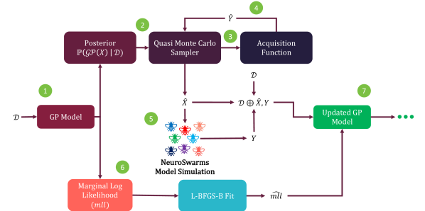
BayesOpt is a technique that allows for the construction and sequential optimization of surrogate models to represent the objective performance of more complex models [31, 32, 33]. Optimizing surrogate models can be beneficial in scenarios where executing a complex model is slow and/or computationally expensive. These surrogate models can be deployed to predict the performance of the underlying complex model at untested parameter values without actually running it. Figure 1(a) illustrates the BayesOpt process we use to optimize the NeuroSwarms model.
Specifically, in our work we explore a category of BayesOpt surrogate models called GP models [11, 35, 36]. GP models are probabilistic parametric models that learn to estimate objective performance from limited observations [12]. GP models iteratively learn a probabilistic mapping from input parameter points to the desired output objective function value ( in the case of our scalar objective) expressed as [37, 38]. GP models estimate this mapping by assuming the complex model is distributed according to a GP:
| (3) |
where and are the mean and covariance kernel on , and is set of training points used to seed the GP model. The posterior distribution of candidate set , where is the number of candidate points, conditioned on data is a multivariate normal .
The other key component of the BayesOpt process is an acquisition function, which is used to navigate the underlying complex model’s parameter space. Acquisition functions define a strategy to manage the trade-off between exploring the parameter space and exploiting promising regions of the parameter space that yielded improvement in previous samples [39]. The acquisition function’s parameters are optimized by evaluating it on . Formally, an arbitrary acquisition function () can be expressed as follows:
| (4) |
where is the utility function and is a composite objective function [40]. However, analytical expressions are not always available for arbitrary or , which is why MC integration is used to approximate the expectation through sampling , resulting in:
| (5) |
The approximated acquisition function uses number of MC samples used to approximate . We experiment with a pair of MC acquisition functions q-Expected Improvement (qEI) and Noisy q-Expected Improvement (qNoisyEI), compared against random search. qEI can be expressed as:
| (6) |
where batches are sampled from the joint posterior, whereby the improvement over the current best observed objective function value (), assuming noiseless observations, is calculated for each sample, and the maximum is taken for each batch and averaged across the number of MC samples. As in the acquisition approximation, , qEI approximates the posterior with .
Similarly, qNoisyEI [41] operates on the same principle of averaging the maximum improvement for batches of samples, except it does not assume noiseless observations such as being the best objective function value. Instead,
| (7) |
where , is an approximation of the posterior distribution of previously observed parameters .
3.2 Objective Function
We introduce an objective function to evaluate the performance of a multi-agent model (e.g. NeuroSwarms) in time-optimal cooperative reward capture. The objective function quantifies how quickly the swarm of agents can forage and collectively capture all the rewards in a given environment. Let be the number of cooperatively captured rewards where a reward is captured if at any time-step at least number of agents were simultaneously colocated within a defined radius from the reward. This objective function can be expressed as a loss,
| (8) |
which is updated at each time-step, where is the total number of time steps, until all rewards have been captured. The swarm is encouraged to complete the task quickly since grows for each time-step needed to capture all the rewards. If the swarm is not able to capture all the rewards in the environment, will be set to the maximum number of time-steps allowed for the simulation and the loss will only reduce for each . Objective values range from , with the theoretical best value at zero.
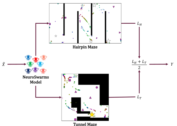
When evaluating NeuroSwarms simulation performance for a given set of parameters, generalizable performance is also taken into account. Each simulation constitutes a play-through of the Hairpin and Tunnel mazes (see Figure 1(b)) where the objective performance is and , respectively. Thus, the overall performance, , of candidate set parameters is calculated as the average:
| (9) |
3.3 GP Surrogate Training
We use the BayesOpt software framework BoTorch [38] to implement the overall BayesOpt process described in Figure 1(a). The training process starts by taking an initial set of training examples is used to initialize the GP model. The resulting posterior distribution is then sampled using a batched quasi-MC sampler, where an acquisition function determines the set of future candidate NeuroSwarms parameters based on the perceived utility for each set of parameters. The sampled parameters are bounded by the range limits outlined in Table 1. Next, the set of future candidate NeuroSwarms parameters undergo a NeuroSwarms model simulation which results in a NeuroSwarms performance evaluation . Afterwards, the pair and are incorporated into which will be used to initialize the GP model in the next optimization step. The GP model is optimized by first computing its marginal log likelihood -acting as a loss function- applied to and then fitting the hyperparameters of the GP model using the limited memory Broyden–Fletcher–Goldfarb–Shannon algorithm. The fitting process also results in an updated marginal log likelihood used for the next optimization step. The whole optimization process is repeated for epochs, where is determined by satisfactory convergence.
Training examples and NeuroSwarms model simulations are formed by running simulations according to Figure 1(b), where a set of randomly chosen parameters (in this case represented by ) are used to initialize the NeuroSwarms model and a unique simulation is performed on the hairpin and tunnel mazes separately. NeuroSwarms model performance is evaluated for each environment according to Equation 8 to encourage cooperative foraging, which is then averaged to produce the generalized foraging performance . Simulations are conducted on two unique mazes to evaluate how well the results in NeuroSwarms model performance that generalizes across environments.
3.4 Convergence Metrics
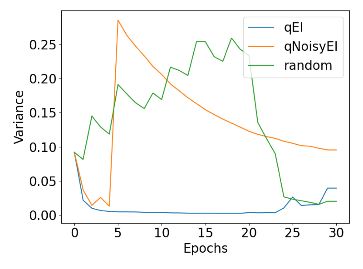
In order to understand when GP model optimization has converged to a satisfactory conclusion we use two convergence metrics. One evaluation criteria would be the maximum posterior variance for the epoch compared with all previous epochs, which can be expressed as follows:
| (10) |
This stopping criteria suggests that when the GP model’s posterior variance is no longer increasing when compared to previous training iterations, then training should stop because the GP model is having minimal change which is undesirable. Dissimilarity is another metric that couples well with the maximum posterior variance because it measures the lack of change in the selection of future candidate parameters when compared to previously simulated parameters . Dissimilarity is defined as:
| (11) |
When a given GP model’s dissimilarity approaches zero the set of parameters from a given epoch is most similar to the set of parameters selected by the acquisition function on the last epoch of training. In order to prevent division by zero, we choose to take the maximum of the product of norms and a constant . Overall, the two convergence metrics evaluate the change of the GP model in terms of its posterior variance or MC sampled , which correspond to improvement in the descriptive capability of the GP model’s posterior. Moreover, a descriptive GP model posterior is essential to understanding the performance of NeuroSwarms parameters in parameter space.
3.5 Visualizing The Parameter Space
Estimating the performance of NeuroSwarms on a set of parameters via a GP model is useful, but understanding which parameters to choose is equally important. Providing a method of visualizing performance across the parameter space facilitates understanding the impact of regions of the parameter space on performance. A visualization tool can allow for the discovery of pockets of high performing parameter sets that solve the foraging problem in unique ways. Since the multivariate norms are entangled in dependencies between all parameters, we turn to UMAP [42] to embed the high dimensional parameter space manifold into a 2D representation. The low dimensional representation is trained to spatially cluster the parameter space such that size sets of parameters are grouped together if they are similar numerical values, and are pushed apart if they are numerically distant from each other. This results in a simple visual representation of where each point can be colored by the corresponding or any of the corresponding parameter values associated with said point. We use this visual tool to qualitatively evaluate the performance of the GP model in approximating the NeuroSwarms model’s performance by selecting a point in UMAP space that has high performance (large ) and matching that point to each of the corresponding parameter values from the parameter set ().
4 Results and Discussion
We present experiments illustrating the use of Bayesian Optimization to tune the parameters of a neuroscience-inspired swarming model, NeuroSwarms [24], tasked with cooperatively capturing multiple rewards in a maze. We train and optimize surrogate GP models to explore and characterize the parameter space of the swarming model using a series of acquisition functions. Then we demonstrate how non-linear dimensionality reduction via UMAP [42] can be used to visualize the parameter space and aid in identifying and selecting a set of parameters that are likely to result in strong model performance. Last, we qualitatively evaluate the performance of selected parameters at generalizing across two distinct environments.
4.1 Gaussian Process Model Training
Manually tuning swarming models, such as NeuroSwarms, can be challenging as small variations in the interdependent parameters (, see Table 1) can dramatically impact model behavior. An optimal set of parameters that allows the NeuroSwarms model to perform successfully on two distinct environments may not be limited to a single set of parameters or may not exist, thus we propose exploring the parameter space in a sample efficient manner using a GP surrogate model. We utilize a MC-based acquisition function to sample the parameter space and optimize the GP model’s predictive performance compared with actual NeuroSwarms simulation results.
An overview of the GP model training process is depicted in Figure 1(a). We optimize GP models on two environments: a hairpin and a tunnel maze (see Figure 1(b)) in order to find dynamical regimes with efficient foraging dynamics.
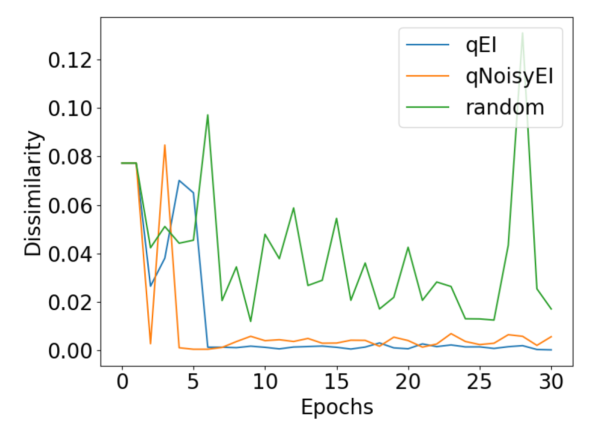
We started the training process of four GP models with an initial set of 24 sets of randomly selected parameters and corresponding simulation results (). Each of the three GP models had one of four acquisition functions that was used to explore the parameter space: expected improvement (qEI), noisy expected improvement (qNoisyEI), and random sampling. GP modeling and training was implemented using the BoTorch [38] framework. Each GP model with a corresponding acquisition function was optimized with MC samples over epochs. All the acquisition functions, except for random, were verified as having converged by the end of the training process using the dissimilarity and posterior variance metrics. Figure 2(a) illustrates that the non-random acquisition function GP models were able to reach near zero dissimilarity during training. Similarly, the posterior distribution’s maximum variance for each of the GP models had reached convergence by the end of the training duration. We stopped training once convergence had been reached to avoid incurring unnecessary simulation computational costs.
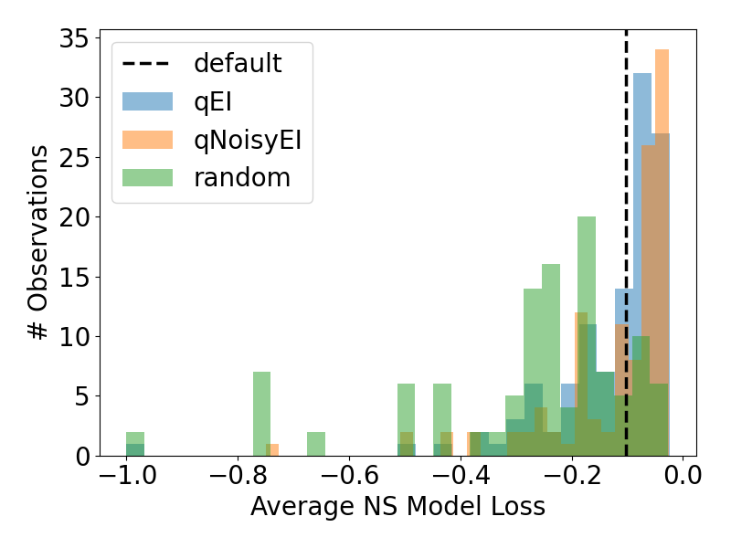
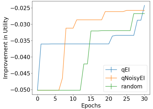
Next, we evaluated how effective each GP model’s acquisition function was at finding regions of the parameter space that maximize the NeuroSwarms objective function. The histogram in Figure 3(a) shows that the qEI and qNoisyEI acquisition function-based GP models were able to locate the most parameter sets that resulted in a high performance NeuroSwarms simulations (closest to 0 are best). For comparison, random parameter selection and the default set of parameters (indicated as default in Figure 3(a)) from Monaco et al. (2020) [24] were both out-performed by the qEI and qNoisyEI acquisition functions-based GP models. The GP models were optimized over fewer parameters with fewer degrees of freedom and still outperformed the default manually tuned parameters. While our objective was to explore the parameter space and not necessarily to find the optimal set of parameters, qEI and qNoisyEI acquisition functions operate on expected improvement in utility which resulted in the most utility improvement when exploring the parameter space over the training process, as depicted in Figure 3(b).
4.2 Qualitative Evaluation
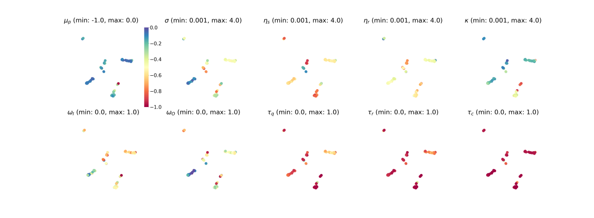
Utilizing the results of the Bayesian optimization process requires a visual representation of the parameter space. Representing an -dimensional parameter space can be challenging, so we elected to use a dimensionality reduction and visualization method called UMAP [42]. UMAP allows the -dimensional parameter space to be reduced to two dimensions, which can then be easily visualized. As illustrated in the top left plot in Figure 4, we were able to assign a color to each low dimensional representation dot based on the corresponding utility value obtained from the GP models’ posterior distribution’s mean value at said position in the parameter space. Similarly, we generated plots for each of the parameters, where points in parameter space were colored based on the corresponding value of said parameter. As a result, we were able to create a visual representation where the highest utility (posterior mean) set of points could be identified as a group, and then individually using the other parallel plots.
Given that the GP model corresponding to the qEI acquisition function had the largest improvement in utility during the training process according to Figure 3(b) and consistently identified high performance sets of parameters (see Figure 3(a)), we used its depiction of the parameter space for further analysis. Figure 4 illustrates that the qEI GP model identified two clusters of sets of parameters that have the highest utility. From the posterior mean plot, we selected one point from the bottom left cluster and we matched it with the same corresponding position in each of the individual parameter plots below. The color bar was then used to identify the numerical value for all parameters, which were then assigned to the NeuroSwarms model for evaluation. In summary, instead of hand tuning on each environment, the BayesOpt process is an illustration of how we simultaneously tuned all parameters for all environments.
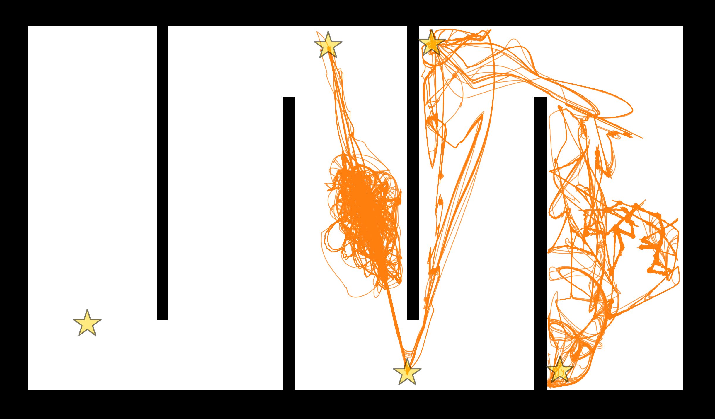
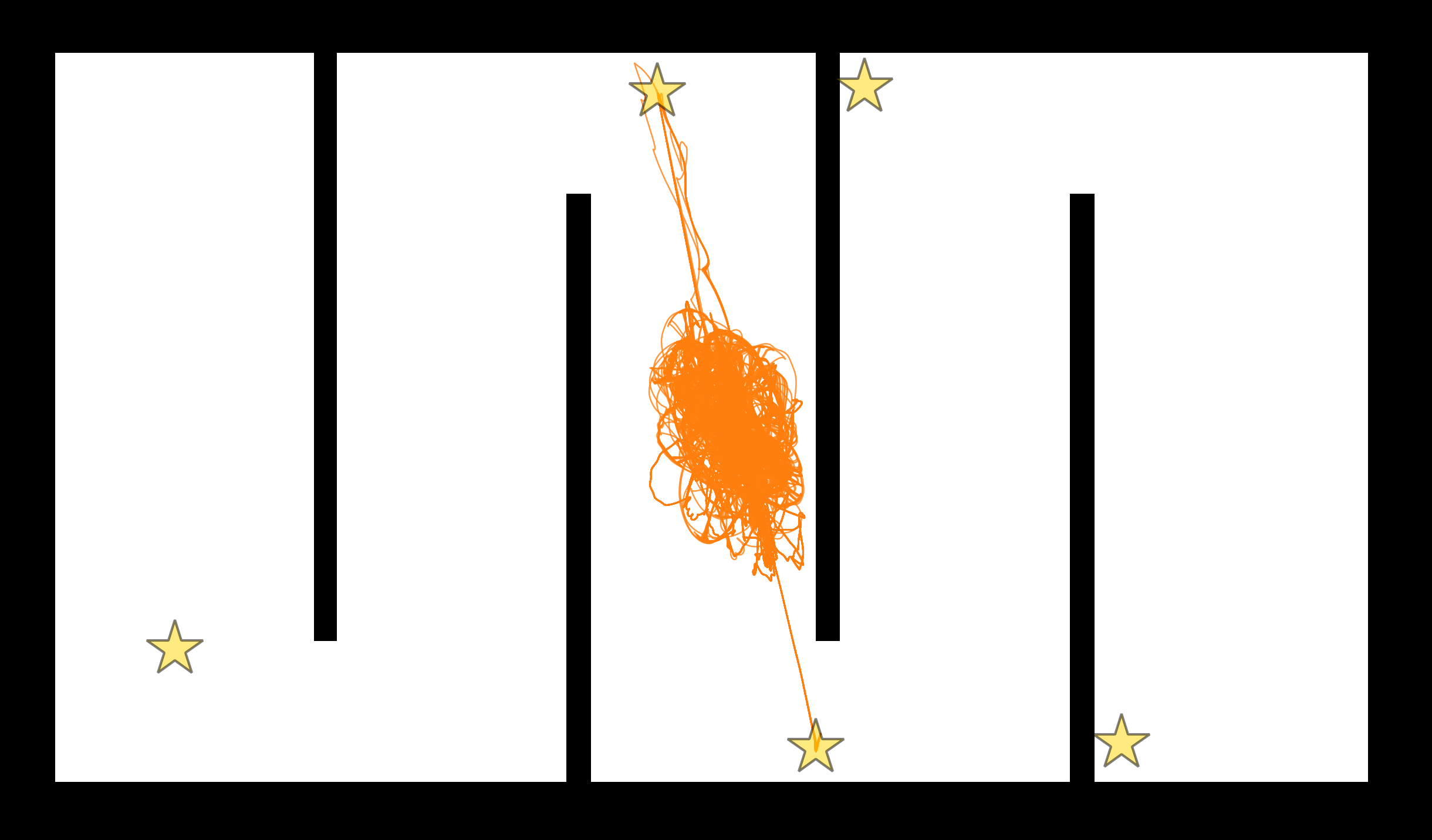
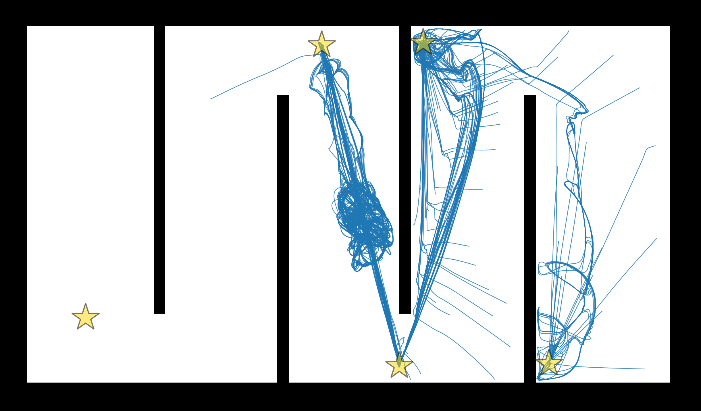
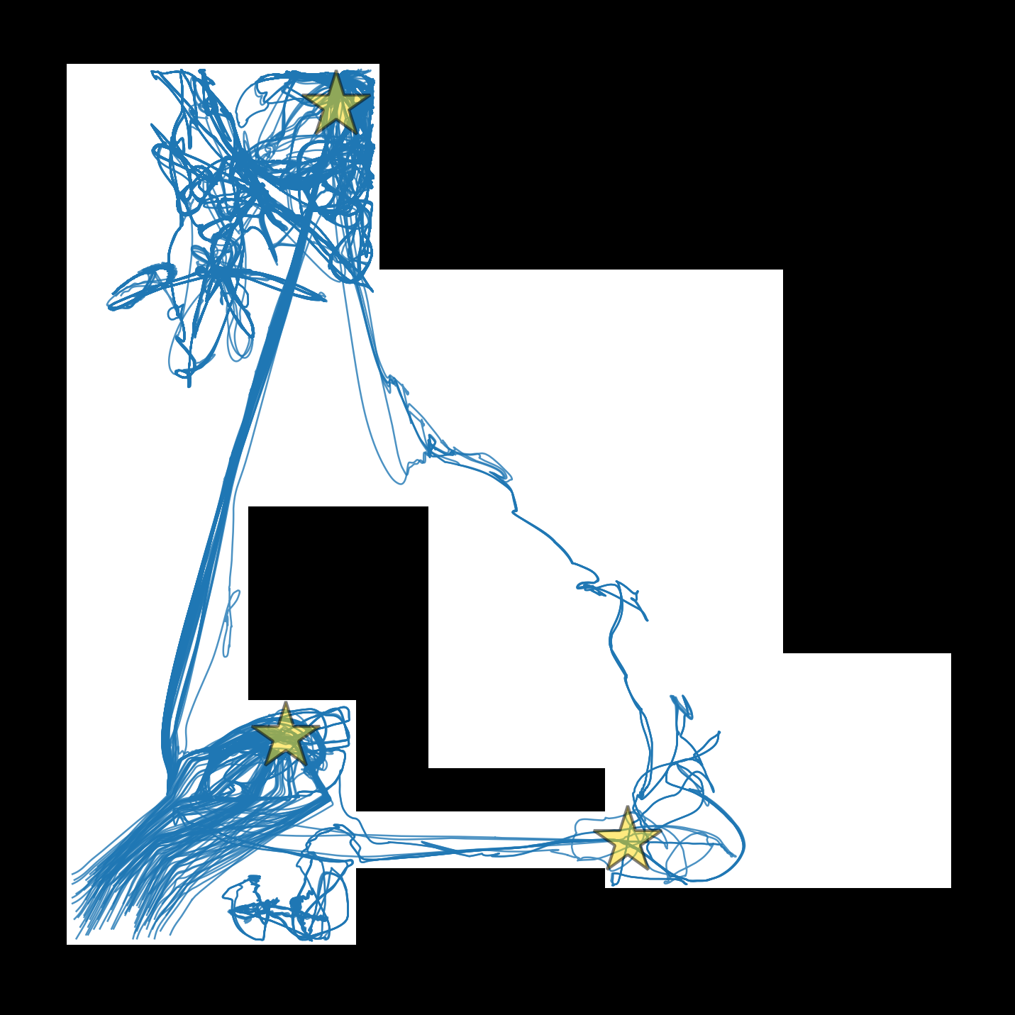
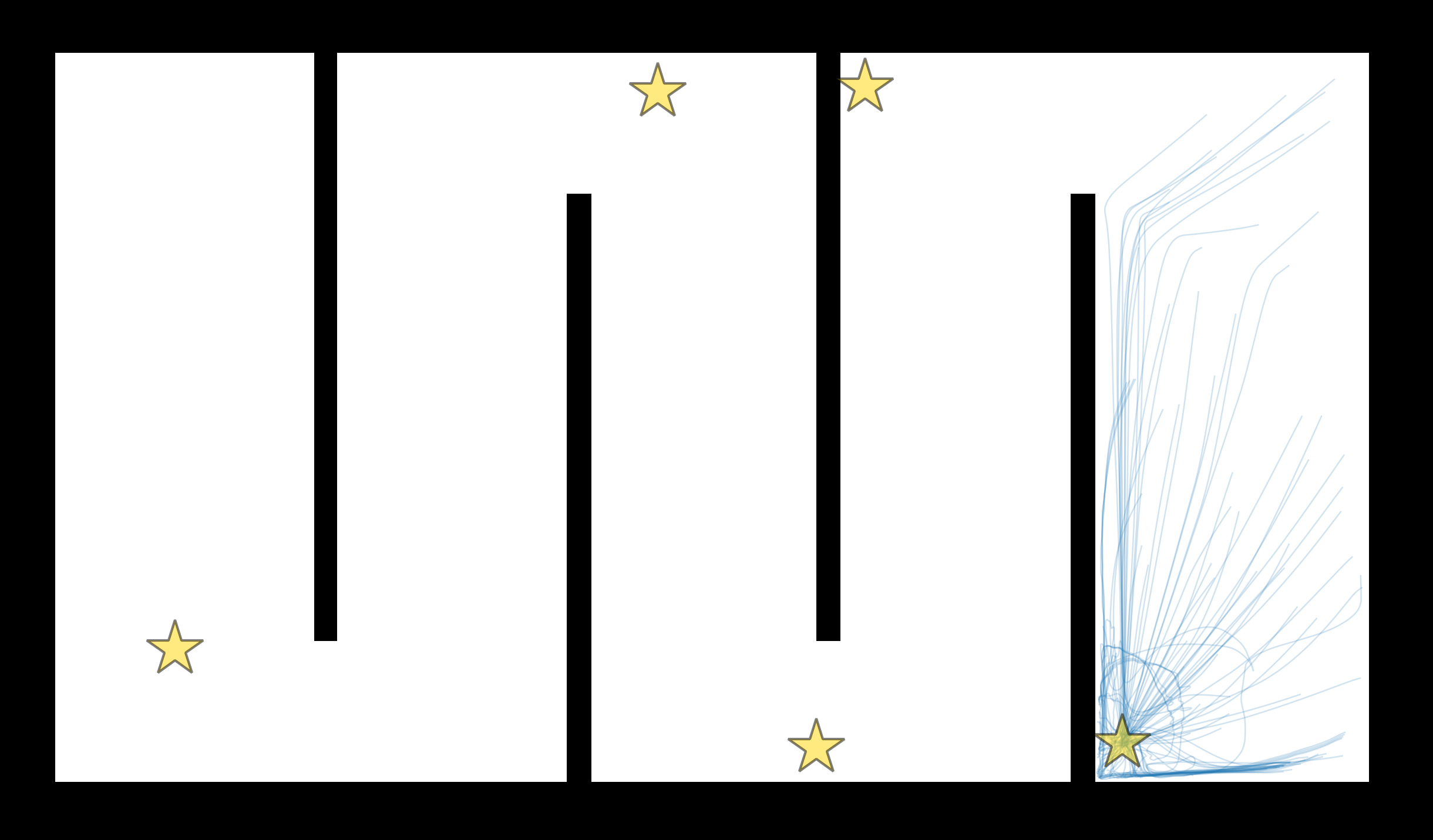
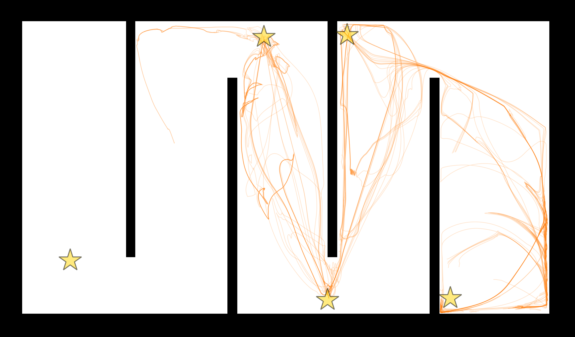
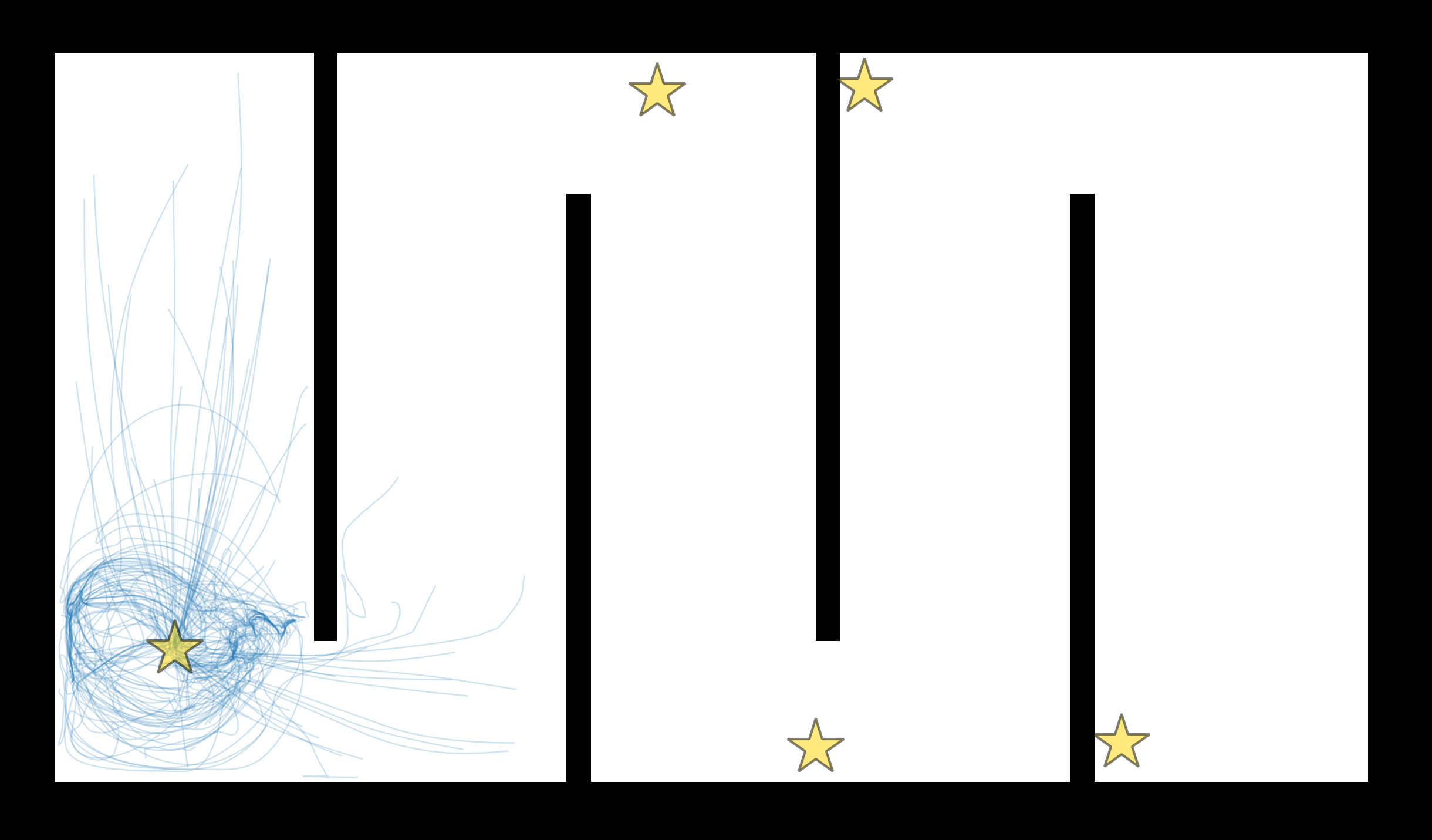
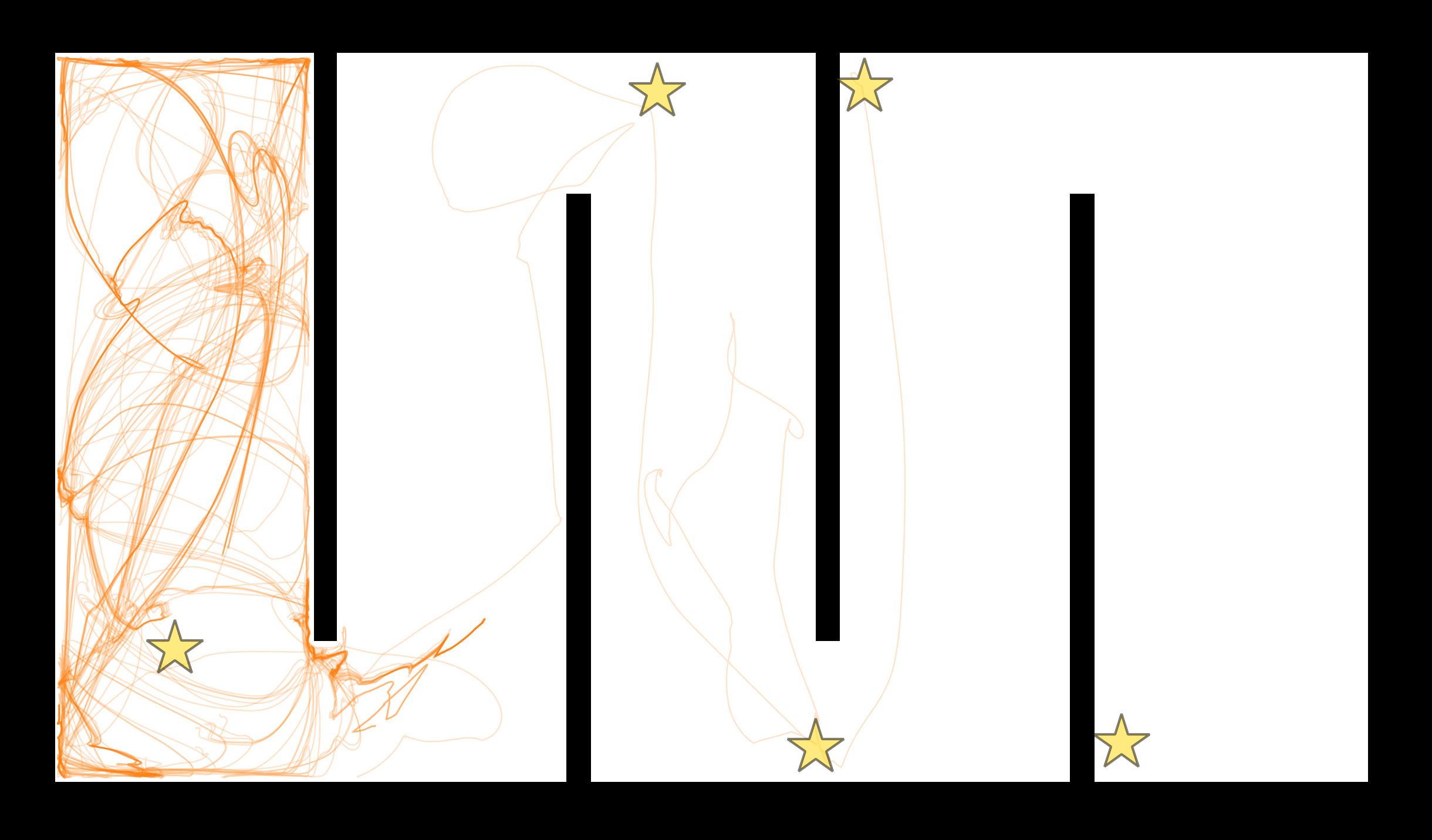
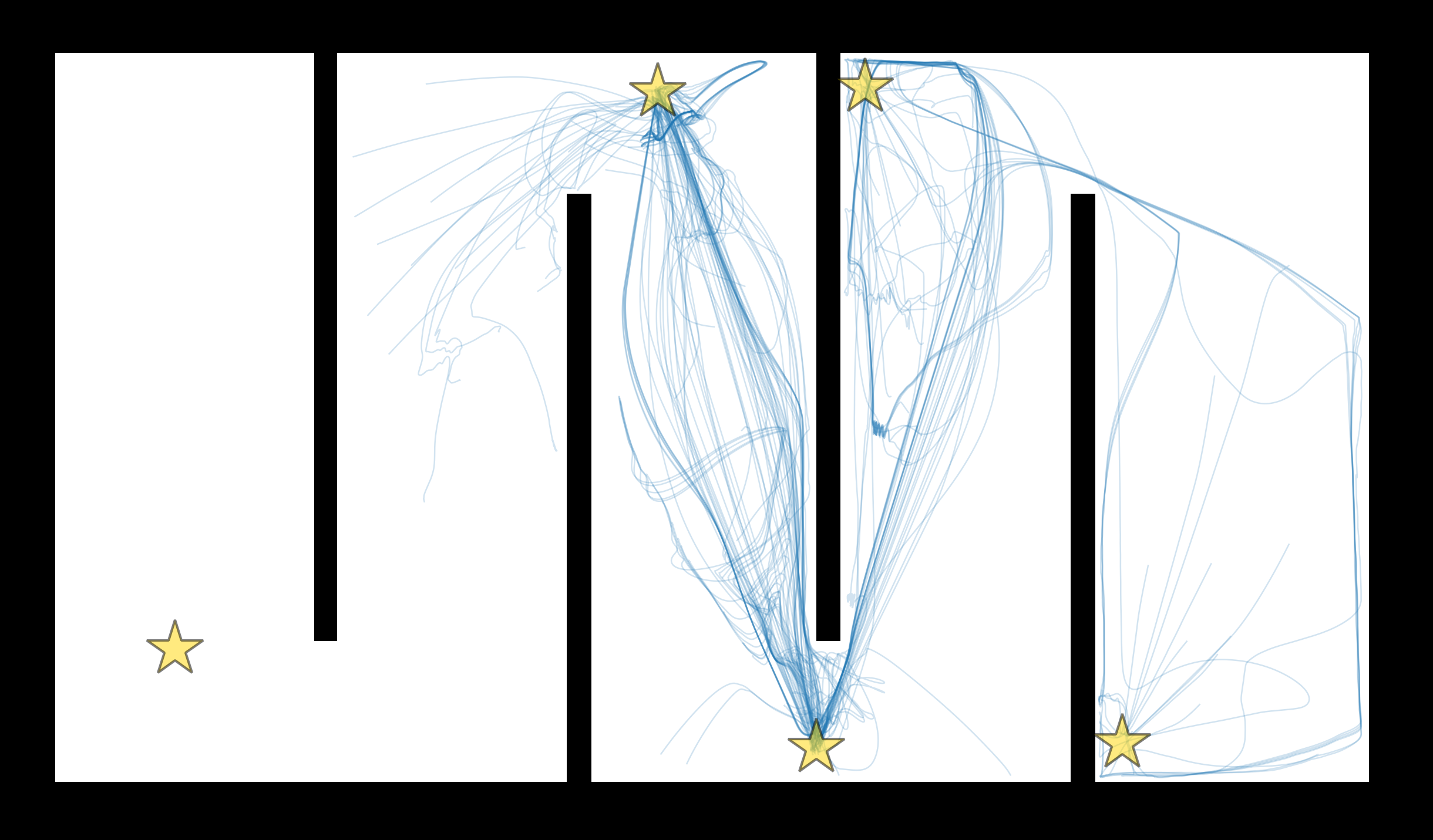
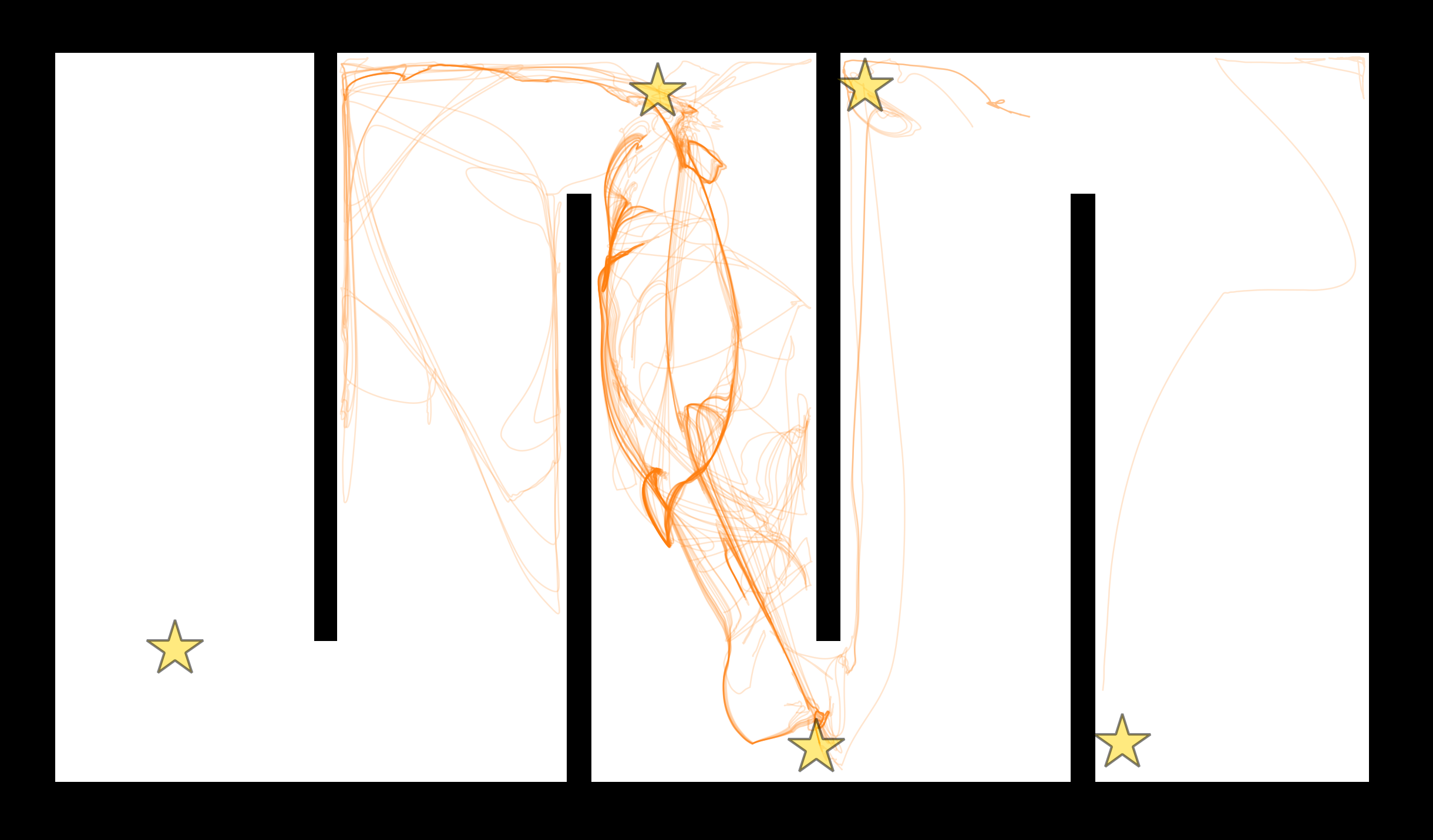
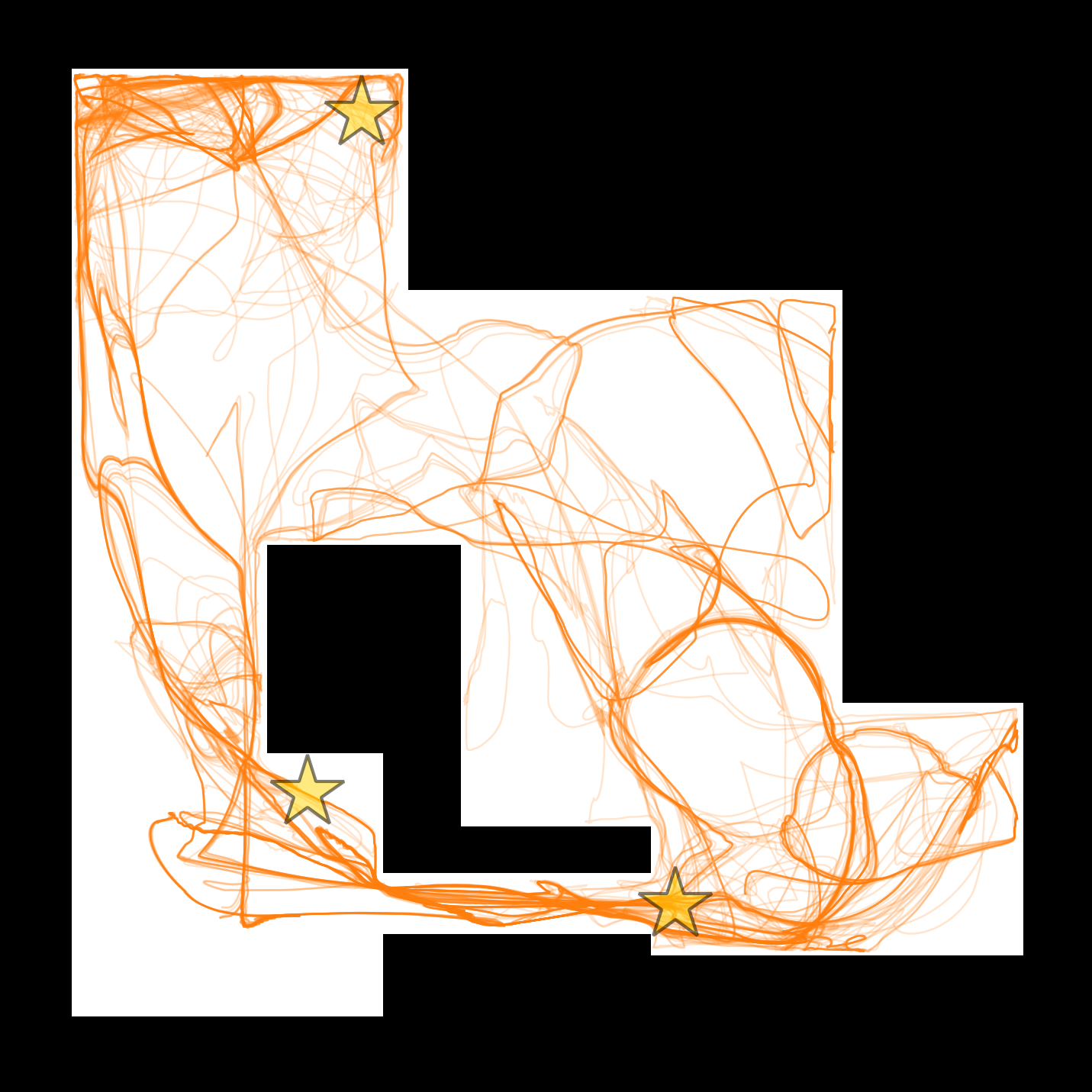
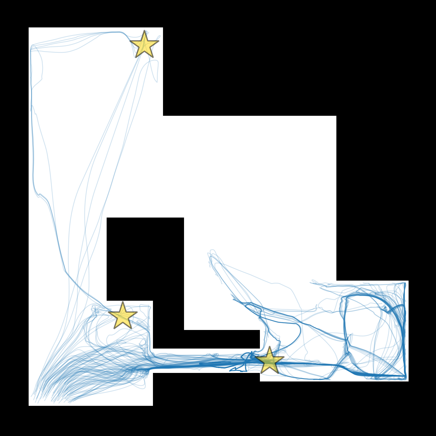
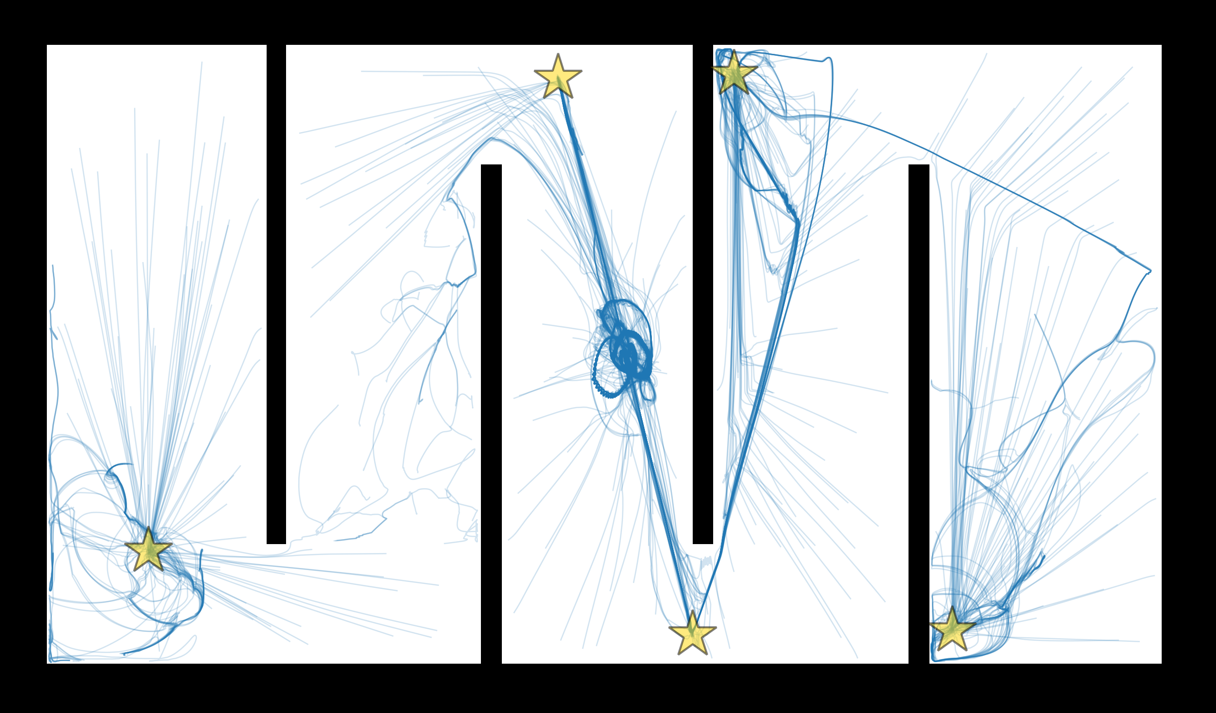
Next, simulations were conducted using the BayesOpt-tuned NeuroSwarms model on both the hairpin and tunnel environments. Trajectory trace plots were generated for the hairpin environment simulation, as depicted in Figure 5. Trajectory traces in blue depict each agent’s movement throughout the simulation up to the point of cooperative capture of a given reward, where only agents that contributed to cooperative capture of said reward were depicted. Orange trajectory traces reflect the behavior of the same set of agents, after the reward had been captured. The transition from swarm goal directed dynamics (in blue) to exploratory swarming (in orange) are best illustrated in Figures 5(e) and 5(f). A portion of the swarm collectively collapse on the 3rd reward and then after capturing the reward immediately disperse to look for other rewards and agents. Agents commence exploring after capturing a reward because NeuroSwarms does not have a global communication system between agents, meaning that agents are not aware if other agents have identified rewards on the other side of the map, occluded by the hairpin walls.
A key feature of our optimization process is the use of an objective function to indirectly evaluate swarm performance at cooperatively foraging and capturing rewards in a distributed manner, but not to directly modify the mechanics of the underlying swarming model. This feature allows the objective function to evaluate swarm on collective social mechanisms, such as distributed cooperation, but the agents of the model can be entirely individualistic. In the case of NeuroSwarms each agent wants to capture all 5 rewards of the hairpin environment, even if other agents have already captured said reward. Figures 5(i) and 5(j) illustrate this scenario, where reward 2 is the last reward to be captured (top center-left), meaning that collectively the swarm has cooperatively captured all 5 rewards. However, since the agents are individually trying to capture all 5 rewards and they have not done so at 25.38s, some agents are shown in Figure 5(j) going back to capture rewards 5 (bottom center) and 1 (top center right).
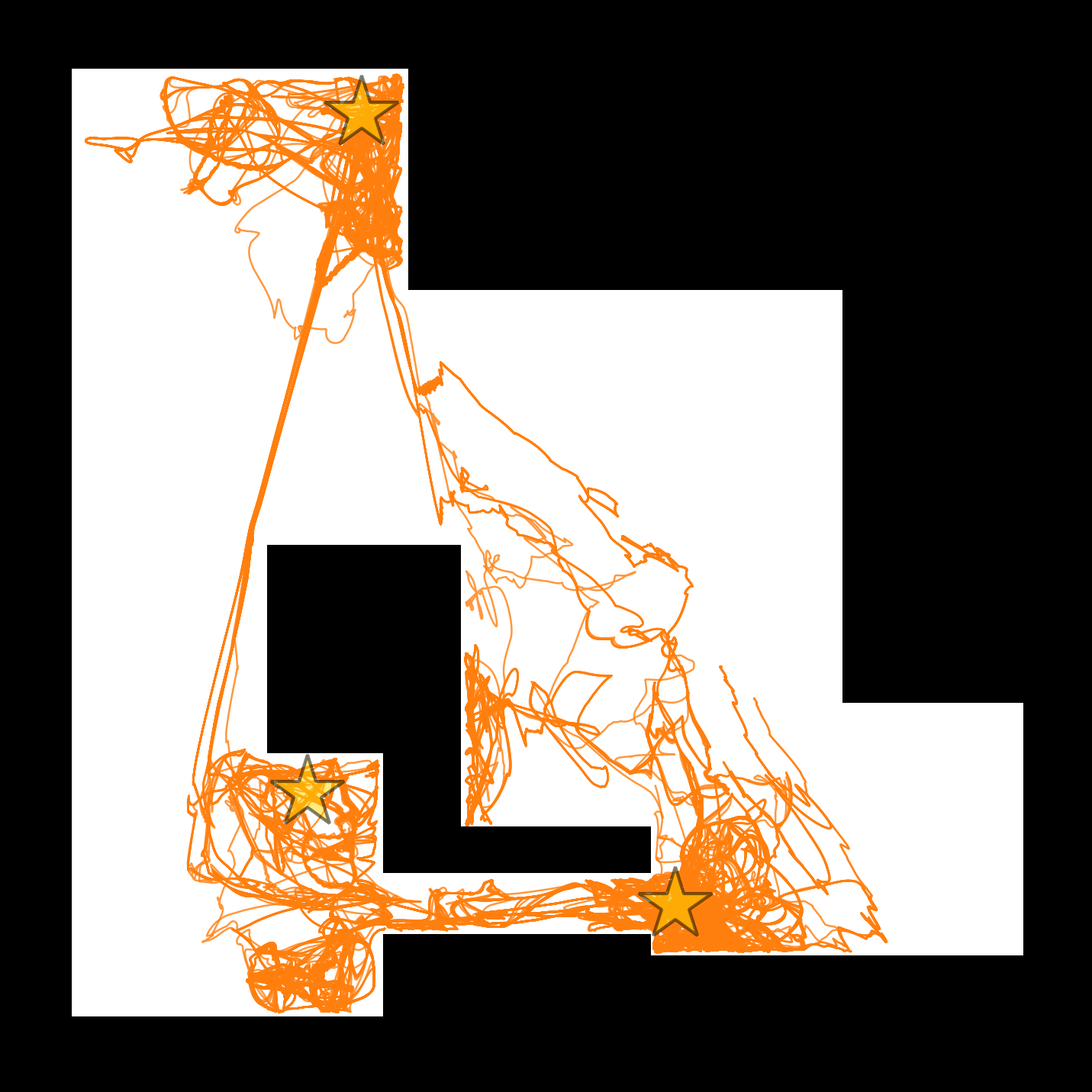
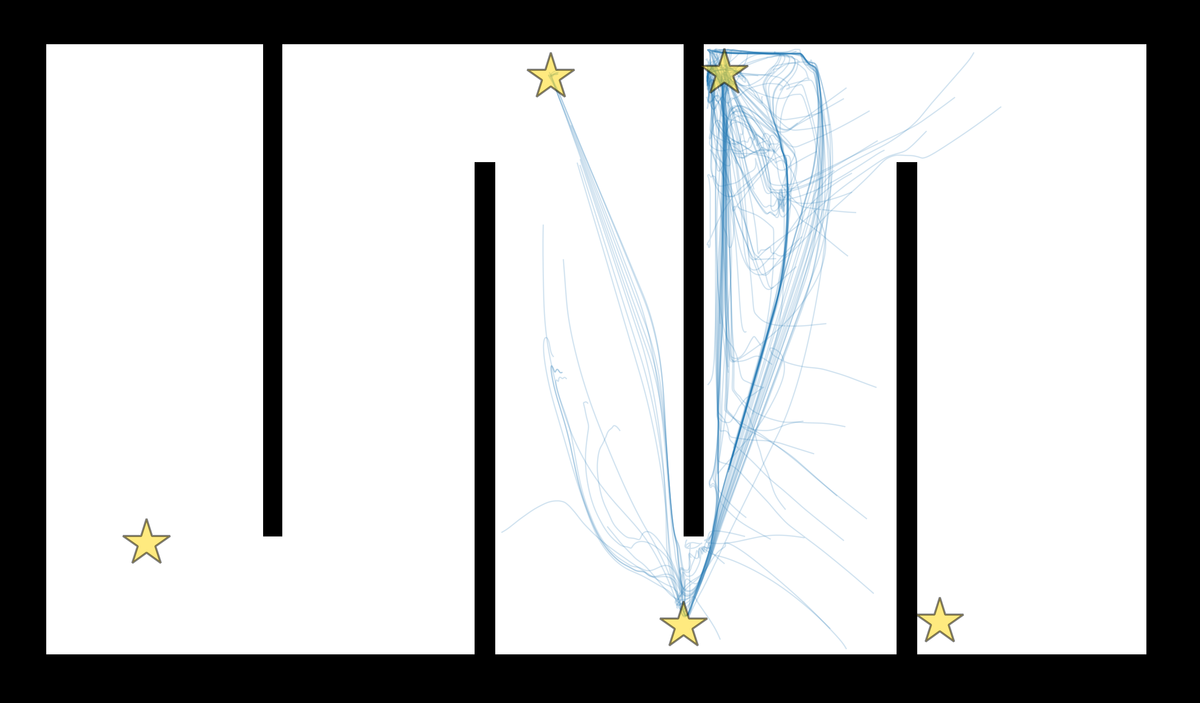
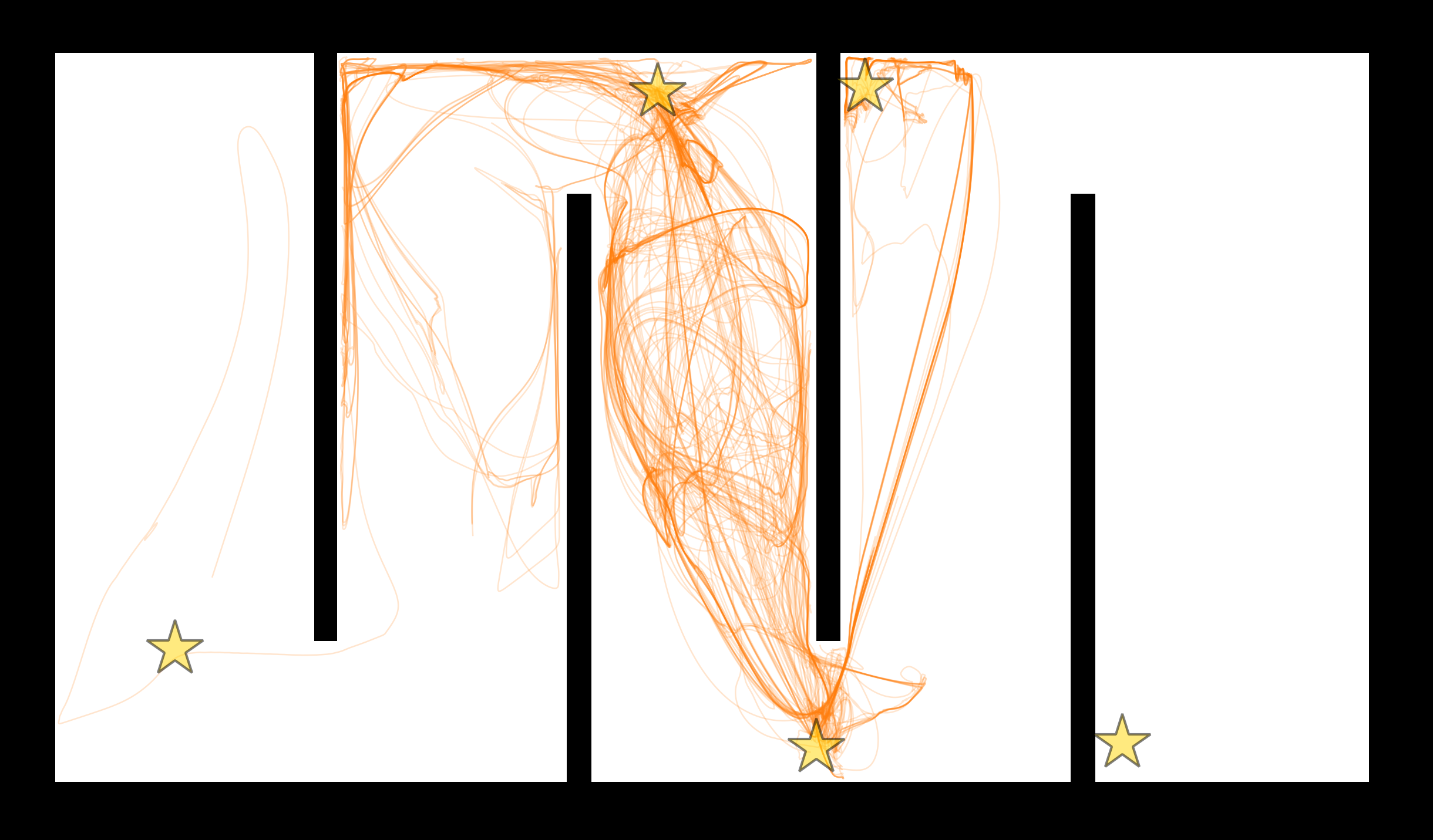
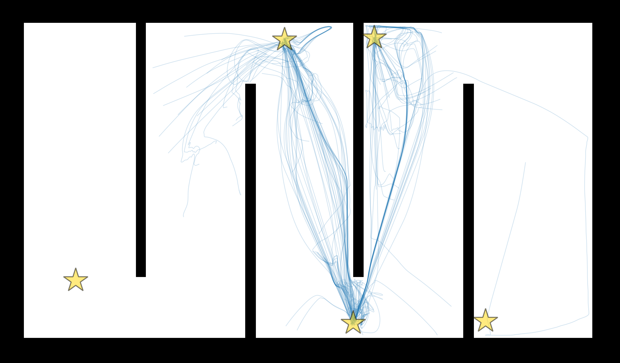
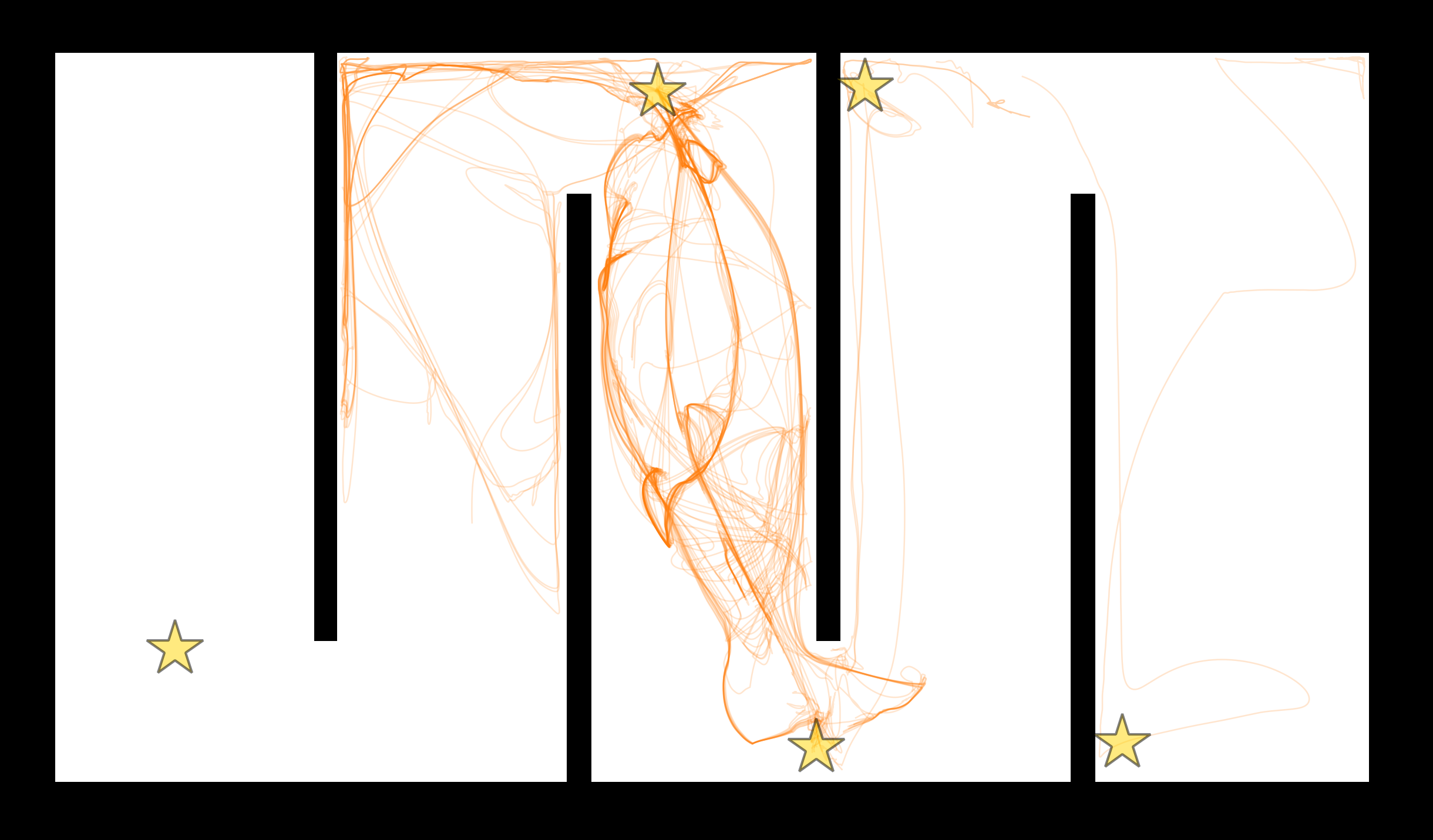
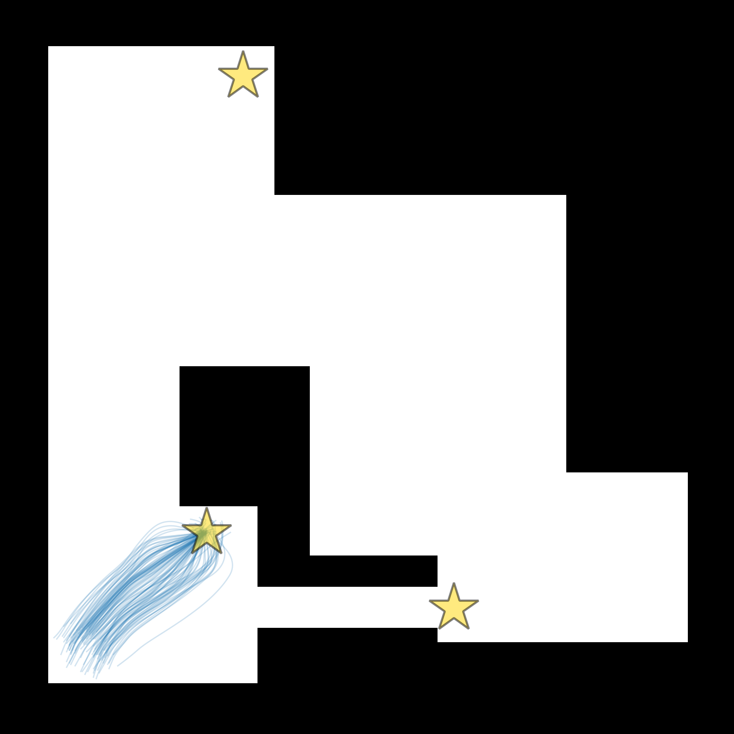
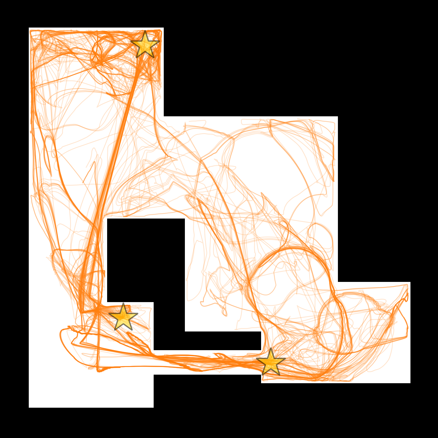
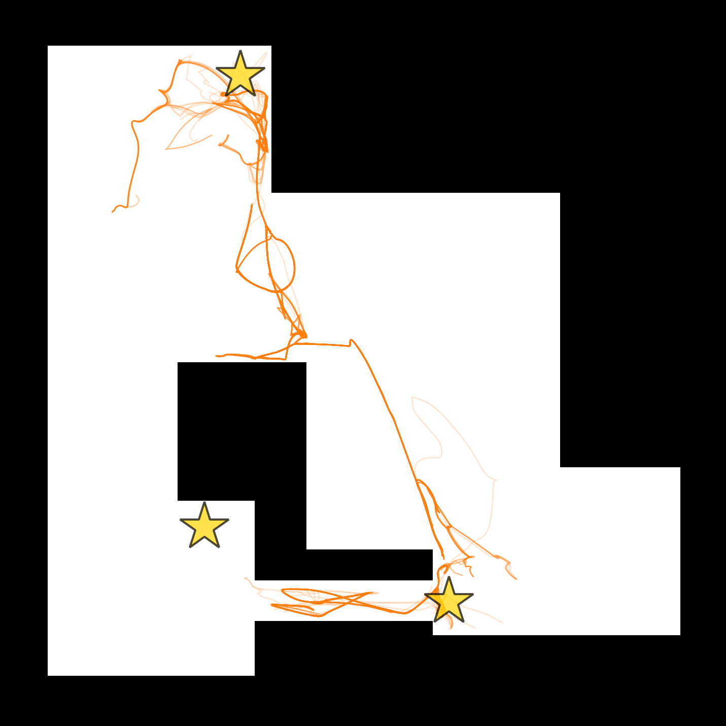
The tunnel environment, shown in Figure 6, provides a scenario whereby the swarm must distribute in order to forage. Unlike the hairpin environment which uniformly at random spawns agents across the entire environment, the tunnel environment spawns all agents in the bottom left corner. As a result, the entire swarm collectively captured a single reward (reward 2 in Figure 6(a) and then had to immediately bifurcate in order to successfully capture the remaining two rewards, see Figures 6(c) and 6(e). This scenario illustrates the success of the parameter optimization process in selecting parameters that encourage flexible swarming that allows a swarm to work in unison and then dissolve in order to seek further rewards. A challenging feature of the tunnel environment is that reward 3 (bottom right) is visible from the spawn position (bottom left) and closer than reward 2, yet has limited accessibility due to the constricting tunnel. Reward 2, on the other hand, is easily accessible yet further away and somewhat occluded after agents transition to reward 1’s (bottom left) position. The substantially faster capture time of reward 1 (5.46s) vs reward 2’s much slower 31.78s illustrates that the parameter choice indirectly prioritized ease of exploration over efficiency in reward capture. Moreover, comparing the before (blue) and after (orange) capture of each of the rewards we identified that agents began to use the large opening in the center of the map only once enough agents had reached the bottom right corner of the map. This phenomenon characterizes the parameter choice as encouraging exploration only once the sub-swarm reaches sufficient membership.

4.3 Exploring Future Parameter Space
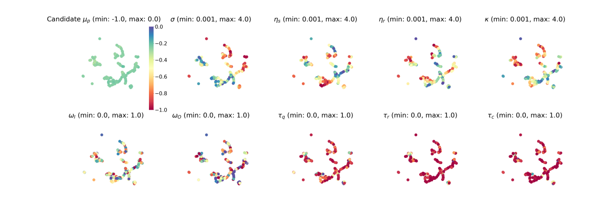
An additional benefit to intelligently exploring the parameter space with acquisition functions is that these trained acquisition functions can then be used to predict the performance of unsimulated regions of the parameter space. In Figure 7 we depict 500 samples from the parameter space chosen by the qEI acquisition function. The samples were evaluated using the trained GP model’s posterior distribution corresponding to the qEI acquisition function. The posterior means (shown in the top left plot) are similar for most points since the qEI acquisition function is targeting regions of the parameter space that are the most likely to produce improvement, which results in samples that are perceived to produce a high objective value (near 0). Following a similar procedure to Subsection 4.2, we selected a set of candidate points from this qEI explored parameter space and simulated the set of parameters on the hairpin and tunnel environments.
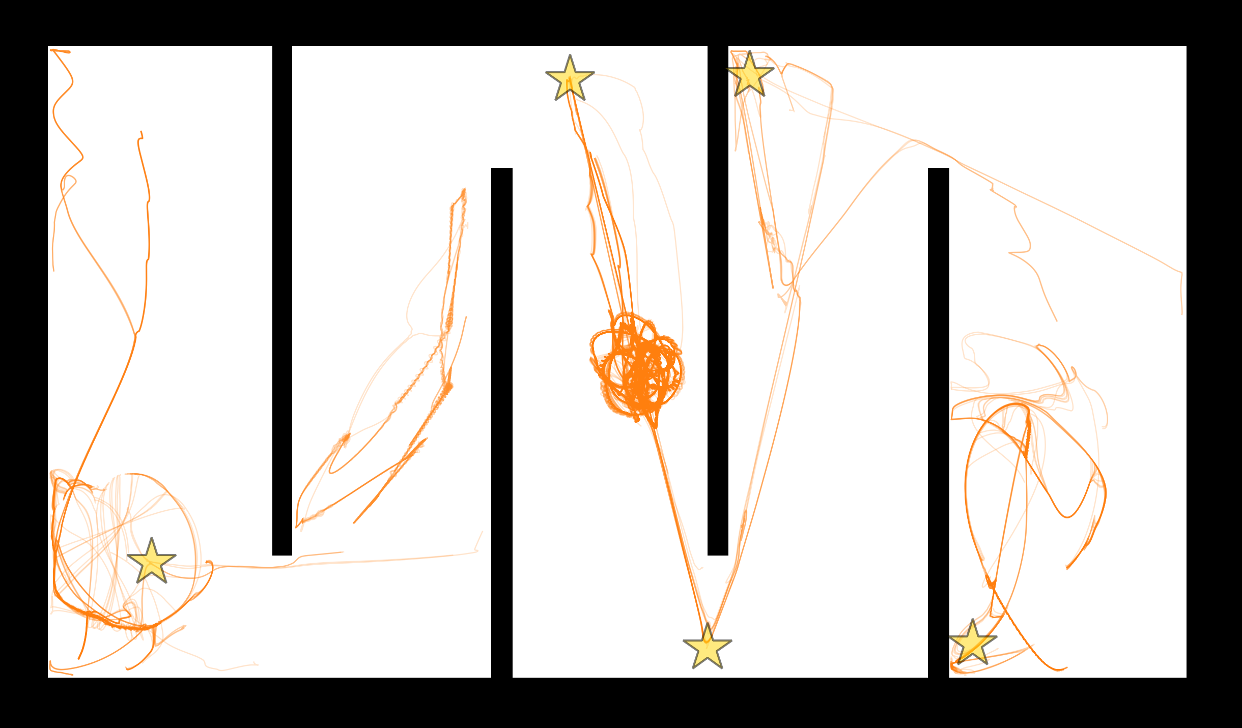

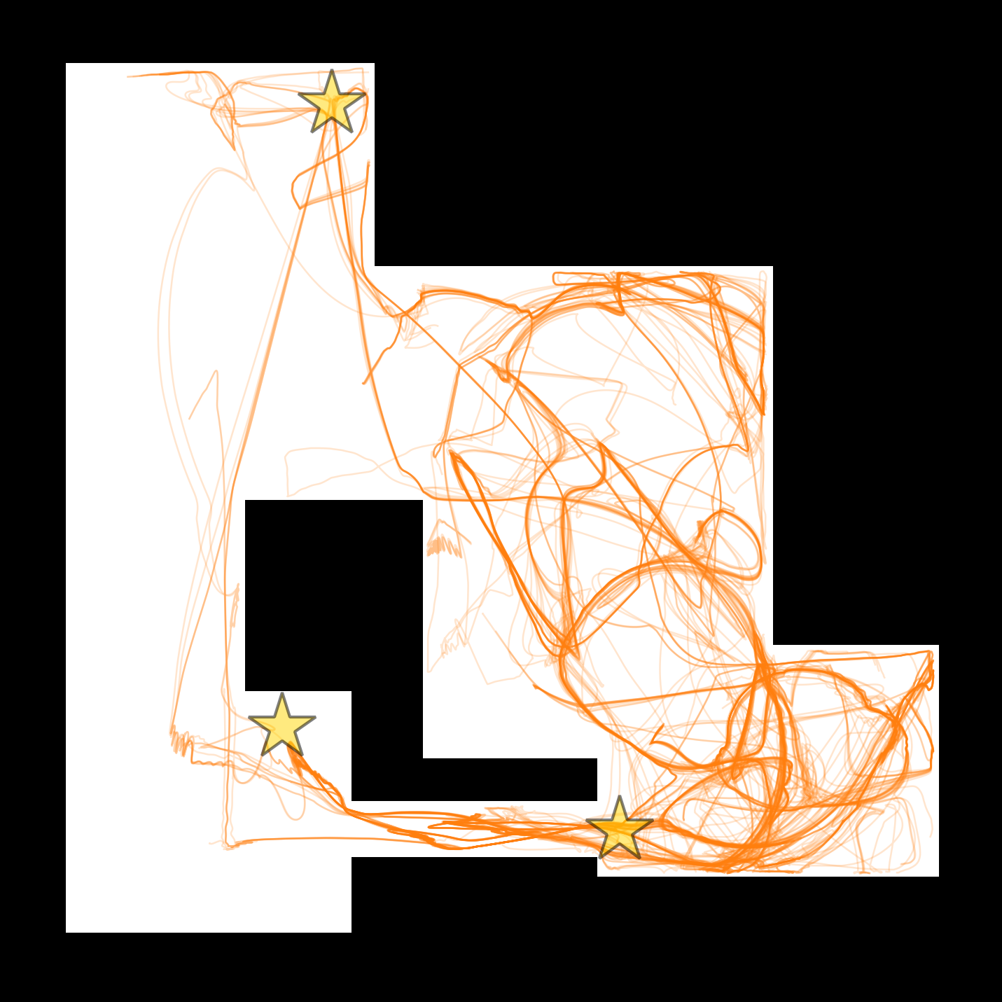
We selected a set of parameters that were predicted to be high performing according to the GP model’s posterior mean and that contained unique selections rarely seen in the parameter space. In particular, we were able to find a combination of parameters where , which is rare since small time constants allow for faster responses which are optimal for fast reward capture. The and the parameters corresponding to exploration were also not at extremes but instead were mid range values. Last, and were not in direct contrast with one another, but were both mid-range values which may be sub-optimal since agents will learn with respect to inter-agent dynamics and reward response will be less impactful. Figure 8 shows trajectory traces of all agents before and after all rewards were cooperatively captured by the swarm on the hairpin and tunnel environments. While all rewards were successfully cooperatively captured by the swarm, as the GP model posterior predicted, the selected set of parameters resulted in slower reward capture. The traceplots show slower (47.44s for hairpin and 66.96s for tunnel) reward capture on both environments compared with the more optimal parameter choice shown in Figures 5 and 6 (25.38s for hairpin 31.78s for tunnel). The slower reward capture is likely attributed to the larger and , which result in slower recurrent and reward updates. However, the swarm exhibited more deliberate cooperation with substantially less erratic exploratory behavior which coincides with neither or being set to the upper limit. In the case where energy consumption related to movement was taken into account, this slower set of parameters would be advantageous as it exhibited effective cooperation with minimal unnecessary exploration.
5 Conclusion
Neuroscience-inspired learning and control methods have become of increasing interest in the domains of Robotics and Artificial Intelligence, in particular for multi-agent control. Here, we presented a method of exploring and visualizing the parameter space of a multi-agent model in a sample efficient manner using BayesOpt. We introduced an objective function for quantifying emergent cooperative foraging for a multi-agent model with no inherent goal-directed cooperative mechanics. Using this objective function, our trained GP model was able to correctly predict the performance of the complex NeuroSwarms model on the task of cooperative foraging across two distinct environments and without simulation on (9) tunable parameters. Training the surrogate GP model was facilitated by directed exploration of the parameter space of the underlying complex model through the use of the qEI or qNoisyEI acquisition functions. The qEI acquisition function was shown to direct exploration towards parameter sets that maximized utility, even over hand-tuned default parameters. Through the use of UMAP [42] we demonstrated a means to visualizing an -dimensional parameter space to identify and select high performing sets of parameters. Lastly, we illustrated the capability of our approach to successfully identify sets of parameters that generalize across environments through evaluation on two environments using the same set of parameters. Overall, our approach serves as a framework by which parameters of complex multi-agent models can be explored and selected to maximize cooperative foraging and reward capture.
In future work, we will consider exploring objective functions that are agnostic to the characteristics of environments (e.g. rewards). Instead, we postulate that the variation of swarm spatial structure can serve as means to evaluate the level of cooperation of a swarm in meeting the goals of an environment, without knowledge of the goals themselves. Such an objective function could extend the flexibility of our approach to operate in any environment and to tasks that exhibit difficult to quantify goals.
6 Acknowledgments
This work was supported by NSF award NCS/FO 1835279 to GMH, KZ, KMS, and JDM; JHU/APL internal research and development awards to AH, GMH, and KMS; and the JHU/Kavli Neuroscience Discovery Institute and JHU/APL Innovation and Collaboration Janney Program provided additional support to GMH.
References
- [1] I. D. Couzin, Collective cognition in animal groups, Trends in Cognitive Sciences 13 (1) (2009) 36–43.
- [2] G. Beni, From swarm intelligence to swarm robotics, in: International Workshop on Swarm Robotics, Springer, 2004, pp. 1–9.
- [3] E. Şahin, Swarm robotics: From sources of inspiration to domains of application, in: International workshop on swarm robotics, Springer, 2004, pp. 10–20.
- [4] M. Brambilla, E. Ferrante, M. Birattari, M. Dorigo, Swarm robotics: a review from the swarm engineering perspective, Swarm Intelligence 7 (1) (2013) 1–41.
- [5] L. Bayındır, A review of swarm robotics tasks, Neurocomputing 172 (2016) 292–321.
- [6] K. Hasselmann, F. Robert, M. Birattari, Automatic design of communication-based behaviors for robot swarms, in: International Conference on Swarm Intelligence, Springer, 2018, pp. 16–29.
- [7] D. S. Brown, R. Turner, O. Hennigh, S. Loscalzo, Discovery and exploration of novel swarm behaviors given limited robot capabilities, in: Distributed Autonomous Robotic Systems, Springer, 2018, pp. 447–460.
- [8] M. Coppola, G. C. de Croon, Optimization of swarm behavior assisted by an automatic local proof for a pattern formation task, in: International Conference on Swarm Intelligence, Springer, 2018, pp. 123–134.
- [9] Y. LeCun, Y. Bengio, G. Hinton, Deep learning, Nature 521 (7553) (2015) 436–444.
- [10] J. D. Monaco, K. Rajan, G. M. Hwang, A brain basis of dynamical intelligence for AI and computational neuroscience (2021). arXiv:2105.07284.
- [11] C. E. Rasmussen, Gaussian Processes in Machine Learning, in: Summer school on machine learning, Springer, 2003, pp. 63–71.
- [12] J. Snoek, H. Larochelle, R. P. Adams, Practical Bayesian Optimization of Machine Learning Algorithms, in: F. Pereira, C. Burges, L. Bottou, K. Weinberger (Eds.), Advances in Neural Information Processing Systems 25, Curran Associates, Inc., 2012, pp. 2951–2959.
- [13] I. Roman, J. Ceberio, A. Mendiburu, J. A. Lozano, Bayesian optimization for parameter tuning in evolutionary algorithms, in: 2016 IEEE Congress on Evolutionary Computation (CEC), IEEE, 2016, pp. 4839–4845.
- [14] V. Nguyen, Bayesian optimization for accelerating hyper-parameter tuning, in: 2019 IEEE Second International Conference on Artificial Intelligence and Knowledge Engineering (AIKE), IEEE, 2019, pp. 302–305.
- [15] I. Roman, A. Mendiburu, R. Santana, J. A. Lozano, Bayesian Optimization approaches for massively multi-modal problems, in: International Conference on Learning and Intelligent Optimization, Springer, 2019, pp. 383–397.
- [16] E. Kieffer, M. Rosalie, G. Danoy, P. Bouvry, Bayesian Optimization to enhance coverage performance of a swarm of UAV with chaotic dynamics (2018).
- [17] A. Rai, R. Antonova, F. Meier, C. G. Atkeson, Using simulation to improve sample-efficiency of Bayesian optimization for bipedal robots, The Journal of Machine Learning Research 20 (1) (2019) 1844–1867.
- [18] F. Berkenkamp, A. Krause, A. P. Schoellig, Bayesian optimization with safety constraints: safe and automatic parameter tuning in robotics, Machine Learning (2021) 1–35.
- [19] K. P. O’Keeffe, H. Hong, S. H. Strogatz, Oscillators that sync and swarm, Nature communications 8 (1) (2017) 1504.
- [20] K. O’Keeffe, C. Bettstetter, A review of swarmalators and their potential in bio-inspired computing, in: Proc.SPIE, Vol. 10982, 2019.
- [21] M. Iwasa, K. Iida, D. Tanaka, Hierarchical cluster structures in a one-dimensional swarm oscillator model, Phys Rev E Stat Nonlin Soft Matter Phys 81 (4 Pt 2) (2010) 046220.
- [22] M. Iwasa, D. Tanaka, Dimensionality of clusters in a swarm oscillator model, Phys Rev E Stat Nonlin Soft Matter Phys 81 (6 Pt 2) (2010) 066214.
- [23] K. O’Keeffe, S. Ceron, K. Petersen, Collective behaviour of swarmalators on a 1D ring (2021). arXiv:2108.06901.
- [24] J. D. Monaco, G. M. Hwang, K. M. Schultz, K. Zhang, Cognitive swarming in complex environments with attractor dynamics and oscillatory computing, Biological cybernetics 114 (2) (2020) 269–284.
- [25] J. D. Monaco, R. M. De Guzman, H. T. Blair, K. Zhang, Spatial synchronization codes from coupled rate-phase neurons, PLoS computational biology 15 (1) (2019) e1006741.
- [26] J. D. Monaco, G. M. Hwang, K. M. Schultz, K. Zhang, Cognitive swarming: an approach from the theoretical neuroscience of hippocampal function, in: Micro-and Nanotechnology Sensors, Systems, and Applications XI, Vol. 10982, International Society for Optics and Photonics, 2019, p. 109822D.
- [27] K. Zhang, Representation of spatial orientation by the intrinsic dynamics of the head-direction cell ensemble: a theory, Journal of Neuroscience 16 (6) (1996) 2112–2126.
- [28] J. D. Monaco, J. J. Knierim, K. Zhang, Sensory feedback, error correction, and remapping in a multiple oscillator model of place-cell activity, Frontiers in Computational Neuroscience 5 (2011) 39.
- [29] G. Buzsáki, Theta rhythm of navigation: link between path integration and landmark navigation, episodic and semantic memory, Hippocampus 15 (7) (2005) 827–840.
- [30] H. T. Blair, A. Wu, J. Cong, Oscillatory neurocomputing with ring attractors: a network architecture for mapping locations in space onto patterns of neural synchrony, Philosophical Transactions of the Royal Society B: Biological Sciences 369 (1635) (2014) 20120526.
- [31] A. O’Hagan, Curve fitting and optimal design for prediction, Journal of the Royal Statistical Society: Series B (Methodological) 40 (1) (1978) 1–24.
- [32] D. R. Jones, M. Schonlau, W. J. Welch, Efficient global optimization of expensive black-box functions, Journal of Global optimization 13 (4) (1998) 455–492.
- [33] M. A. Osborne, Bayesian Gaussian processes for sequential prediction, optimisation and quadrature, Ph.D. thesis, Oxford University, UK (2010).
- [34] C. Zhu, R. H. Byrd, P. Lu, J. Nocedal, Algorithm 778: L-bfgs-b: Fortran subroutines for large-scale bound-constrained optimization, ACM Transactions on Mathematical Software (TOMS) 23 (4) (1997) 550–560.
- [35] C. K. Williams, Prediction with Gaussian processes: From linear regression to linear prediction and beyond, in: Learning in graphical models, Springer, 1998, pp. 599–621.
- [36] D. J. MacKay, Gaussian processes-a replacement for supervised neural networks? (1997).
- [37] K. Krauth, E. V. Bonilla, K. Cutajar, M. Filippone, AutoGP: Exploring the capabilities and limitations of Gaussian process models, arXiv preprint arXiv:1610.05392 (2016).
- [38] M. Balandat, B. Karrer, D. R. Jiang, S. Daulton, B. Letham, A. G. Wilson, E. Bakshy, BoTorch: A Framework for Efficient Monte-Carlo Bayesian Optimization, in: Advances in Neural Information Processing Systems 33, 2020.
- [39] B. Shahriari, K. Swersky, Z. Wang, R. P. Adams, N. De Freitas, Taking the human out of the loop: A review of Bayesian optimization, Proceedings of the IEEE 104 (1) (2015) 148–175.
- [40] J. T. Wilson, F. Hutter, M. P. Deisenroth, Maximizing acquisition functions for Bayesian optimization, arXiv preprint arXiv:1805.10196 (2018).
- [41] B. Letham, B. Karrer, G. Ottoni, E. Bakshy, et al., Constrained Bayesian optimization with noisy experiments, Bayesian Analysis 14 (2) (2019) 495–519.
- [42] L. McInnes, J. Healy, J. Melville, UMAP: Uniform Manifold Approximation and Projection for Dimension Reduction, arXiv preprint arXiv:1802.03426 (2018).
In this section we provide additional technical details on parameters not investigated and observations on the default set of parameters.
Appendix A Constants
Model parameters held constant and used by all NeuroSwarms models are described in Table 2. Additionally, the BayesOpt process across all three acquisition functions included the following constants: 256 MC samples, 30 training epochs with a batch size of 3, and 8 initial training examples to initialize the GP model.
| Parameter | Range | Description |
|---|---|---|
| Number of agents | ||
| Simulation integration time step in | ||
| Duration | Simulation duration in | |
| Maximum kinetic energy in | ||
| Momentum coefficient in | ||
| Swarming inputs gain | ||
| Reward inputs gain | ||
| Sensory cue inputs gain | ||
| Reward contact radius for capture |
Appendix B Default Parameters
In Section 4, we identified that the default set of parameters from Monaco et al. (2020) [24] did not perform as well as the acquisition functions-based GP models. We showed, in Figure 3(a), the superior objective function loss performance of the qEI and qNoisyEI the acquisition functions-based GP models over the default parameters. To further illustrate this discrepancy in fast reward capture performance, we ran a simulation using the set of parameters from Monaco et al. (2020) specific to the hairpin environment, shown as trajectory plots in Figure 9, and then repeated this process for the tunnel environment (see Figure 10).
The manually-tuned default parameters poor objective function loss performance can be attributed to the default swarm’s slow reward-capture. The qEI-tuned swarms was able to capture all five rewards on the hairpin environment in 25.38s, as shown in Figure 5(i), where as the sluggish manually-tuned default swarm, shown in Figure 9(i), took 41.02s. The default parameters favor very high levels of reward exploration with a , but low spatial exploration () and equally low inter-agent dynamics and reward response (). This combination of parameters encourages exploration but poor cooperation, which drastically increased the time-to-capture for all five rewards. This slow reward capture behavior is further exacerbated on the tunnel environment, shown in Figure 10(e), where the default parameter swarm took 175.42s to capture all three rewards. For comparison, the qEI-tuned swarm was able to capture all three rewards, see Figure 6(e), faster than the default swarm could capture two rewards (34.88s from Figure 10(c)). Furthermore, a 175.42s all reward capture time is not even permitted for any of the GP-based methods as training criteria cuts off simulations at 120s. If maximum simulation time limits were imposed on the default model, it would have only capture two of the three rewards. Overall, these results illustrated the importance of utilizing automated parameter tuning approaches like BayesOpt for parameter optimization instead of depending on default parameters used by prior works.