Abstract

This paper considers the problem of estimating high dimensional Laplacian constrained precision matrices by minimizing Stein’s loss. We obtain a necessary and sufficient condition for existence of this estimator, that consists on checking whether a certain data dependent graph is connected. We also prove consistency in the high dimensional setting under the symmetrized Stein loss. We show that the error rate does not depend on the graph sparsity, or other type of structure, and that Laplacian constraints are sufficient for high dimensional consistency. Our proofs exploit properties of graph Laplacians, the matrix tree theorem, and a characterization of the proposed estimator based on effective graph resistances. We validate our theoretical claims with numerical experiments.

1 Introduction

Graph based algorithms are becoming increasingly popular in application domains where unstructured and irregular data are pervasive, including signal and image processing (Shuman et al., 2013; Ortega et al., 2018), and machine learning (Von Luxburg, 2007; Bronstein et al., 2017).

In graph based data analysis, observations are located at the nodes (or vertices), while the graph structure and edge weights represent affinity relations between the nodes. A fundamental problem is estimation of graph structure and edge weights from nodal observations. Earlier approaches were based on sparse inverse covariance matrix estimation (Dempster, 1972; Lauritzen, 1996; Friedman et al., 2008; Rothman et al., 2008). More recently, there has been growing interest in estimating Laplacian constrained inverse covariance (precision) matrices (Lake and Tenenbaum, 2010; Slawski and Hein, 2015; Egilmez et al., 2017; Dong et al., 2019; Mateos et al., 2019; Tugnait, 2021). This approach can benefit from developed statistical and graph theories. For example, in the Gaussian case, the entries of the precision matrix correspond to partial correlations (Lauritzen, 1996), while additionally, the spectral decomposition of the Laplacian can be interpreted as a Fourier basis for signals on graphs (Shuman et al., 2013; Ortega et al., 2018; Ortega, 2022).

In this work, we consider undirected graphs with $p$ nodes, and study estimation of the combinatorial graph Laplacian (CGL) matrix from signals $\{{\bf x}_{1},\cdots,{\bf x}_{n}\}\subset{\mathbb{R}}^{p}$, via the CGL estimator (CGLE):

$$\widehat{{\bf L}}=\operatorname*{arg\,min}_{{\bf L}\in{\cal L}_{p}({\cal E})}-\log{\hbox{det}}^{\dagger}\left({\bf L}\right)+\operatorname*{tr}({\bf L}{\bf S}).$$ (1)

Here ${\cal L}_{p}({\cal E})$ is the set of CGL matrices of connected graphs with edge set contained in ${\cal E}$, the product of non zero eigenvalues is denoted by ${\hbox{det}}^{\dagger}$, and ${\bf S}\coloneqq n^{-1}\sum_{i=1}^{n}{\bf x}_{i}{\bf x}_{i}^{\top}$ is the sample covariance matrix. When the signals $\{{\bf x}_{i}\}$ are i.i.d., with zero mean and population covariance matrix $\hbox{\boldmath$\Sigma$}^{\star}=({\bf L}^{\star})^{\dagger}$, (1) is the maximum likelihood estimator of a Gaussian Markov random field with Laplacian constrained precision matrix (L-GMRF) (Lauritzen, 1996; Egilmez et al., 2017; Ying et al., 2020). This estimator also promotes smooth signal representations, essential for signal processing and learning on graphs (Dong et al., 2020; Hu et al., 2021).

In applications such as portfolio selection and gene expression analysis (Cai et al., 2011; Agrawal et al., 2019), the dimension $p$ can be much larger than the sample size $n$. Hence, estimators that perform well and are consistent in this regime have become increasingly attractive. Traditional precision matrix estimation exploited sparsity to achieve high dimensional consistency, and guarantee existence of the precision matrix estimator (Cai et al., 2011; Rothman et al., 2008). It has been shown that when Laplacian constraints are used, various Laplacian estimators exist under milder conditions (Slawski and Hein, 2015; Ying et al., 2021). Consistency in the high dimensional setting has been proven for the generalized graph Laplacian estimator (Soloff et al., 2020), without sparsity assumptions. While for the CGLE case, available results assume graph sparsity (Rabbat, 2017; Ying et al., 2020, 2021).

In this paper we study existence and high dimensional consistency of the CGLE. Our contributions can be summarized as follows:

• We obtain a necessary and sufficient condition for existence of the CGLE (Theorem 1). This condition reduces to checking whether a certain data dependent graph is connected.

• We prove that the CGLE is consistent in the high dimensional setting ($p>n$) under the symmetrized Stein loss (Stein, 1975; Ledoit and Wolf, 2018) with a rate ${\cal O}(\sqrt{\log(p)/n})$ (Theorem 3).

• We prove that tree structured graphs can be estimated at the faster rate ${\cal O}(\log(p)/n)$ (Theorem 4).

Our proofs are relatively simpler than recent works studying existence of the CGLE, and consistency in the Frobenius norm (Ying et al., 2020, 2021). An essential part of our analysis is based on a characterization of the CGLE by Pavez and Ortega (2019) that uses effective graph resistances and the matrix tree theorem (Klein and Randić, 1993; Xiao and Gutman, 2003; Ellens et al., 2011). Unlike other Laplacian and (inverse) covariance estimators that require some structural assumption such as sparsity, bounded degree, or bandable structures to achieve high dimensional consistency (Cai et al., 2016; Rabbat, 2017; Ying et al., 2020, 2021), our results are able to achieve the rate ${\cal O}(\sqrt{\log(p)/n})$ by exploiting properties of CGL matrices and using the symmetrized Stein loss, without requiring other types of graph structure.

The rest of the paper is organized as follows. In Section 2 we review related work. We introduce notation, and some graph theoretic concepts in Section 3. Our results about existence and consistency are presented in Sections 4 and 5, respectively. We finalize with numerical experiments in Section 6, and conclusions in Section 7.

Table 1: Comparison of key parameters for estimation of Laplacian constrained precision matrices. GGL are the matrices $\{\hbox{\boldmath$\Theta$}\succ 0$, $\theta_{ij}\leq 0,~{}\forall i\neq j\}$. The sample correlation and distant coefficients are $\hat{\rho}_{ij}=S_{ij}/\sqrt{S_{ii}S_{jj}}$, and $h_{ij}=S_{ii}+S_{jj}-2S_{ij}$ respectively. $\rho$ and $\hat{\rho}$ are the largest population and sample correlation coefficients respectively, thus $\rho=\max_{i\neq j}\Sigma^{\star}_{ij}/\sqrt{\Sigma^{\star}_{ii}\Sigma^{\star}_{jj}}$, and $\hat{\rho}=\max_{i\neq j}\hat{\rho}_{ij}$.

Estimator	Existence condition	Optimal weights	Convergence rate
GGL	$\hat{\rho}<1$ (Slawski and Hein, 2015)	$|\hat{\theta}_{ij}|\leq\frac{|S_{ij}|/S_{ii}S_{jj}}{1-\hat{\rho}^{2}_{ij}}$ (Appendix A)	$\frac{1}{1-\rho}\sqrt{\frac{\log(p)}{n}}$ (Soloff et al., 2020)
CGL	$\min_{(i,j)\in{\cal E}}h_{ij}>0$ (Th. 1)	$\hat{w}_{ij}\leq\frac{1}{h_{ij}}$ (Pavez and Ortega, 2019)	$\sqrt{\frac{\log(p)}{n}}$ (Th. 3)

2 Related work

Inverse covariance estimators.

The CGLE is closely related to sparse inverse covariance matrix estimators of the form:

$$\min_{\hbox{\boldmath$\Theta$}\in{\cal S}}-\log{\hbox{det}}(\hbox{\boldmath$\Theta$})+\operatorname*{tr}(\hbox{\boldmath$\Theta$}{\bf S})+\alpha\|\hbox{\boldmath$\Theta$}\|_{1}.$$ (2)

When ${\cal S}$ is the set of symmetric positive definite matrices and $\alpha=0$, (2) is the maximum likelihood estimator (MLE) of the inverse covariance matrix under a Gaussian distribution (Dempster, 1972). When $\alpha>0$, this estimator is known as graphical lasso (Friedman et al., 2008). It was recently proposed to solve (2) for matrices with non positive off diagonal entries, i.e., ${\cal S}$ is the set of M-matrices, also known as generalized graph Laplacians (GGL). The unregularized case ($\alpha=0$ ) was first studied by Slawski and Hein (2015) and the $\ell_{1}$ regularized ($\alpha>0$) by Egilmez et al. (2017); Pavez et al. (2018). The estimator (1) was first proposed by Egilmez et al. (2017). Since then, several algorithms and extensions for estimating CGL matrices have been proposed (Hassan-Moghaddam et al., 2016; Moghaddam and Jovanovic, 2017; Rabbat, 2017; Egilmez et al., 2018; Pavez and Ortega, 2019; Zhao et al., 2019; Kumar et al., 2020).

Existence.

The Gaussian MLE does not exist when $n<p$, unless additional sparsity constraints are imposed on $\Theta$, in which case, existence is guaranteed for $\tau\leq n<p$, for some $\tau>0$ that depends on the graph structure (Uhler, 2012). The graphical lasso always exists for every $n\geq 1$, however note that using this estimator is only reasonable when sparsity is required. In contrast, the generalized graph Laplacian estimator (GGLE) and the CGLE exist with probability one, as long as $n\geq 2$ under mild conditions on the data distribution (Slawski and Hein, 2015; Ying et al., 2021). In particular, the CGLE exists with high probability when ${\cal E}$ is the complete graph and the data follows a Laplacian Gaussian Markov random field distribution (Ying et al., 2021). Unlike previous work, we obtain a necessary and sufficient condition for existence of the CGLE for the more general case that includes edge constraints.

Consistency and regularization.

It is well known that for many optimization problems, adding $\ell_{1}$ regularization produces sparse solutions. In particular, as the regularization parameter $\alpha$ is increased, the regularized MLE solution (2) becomes more sparse, for both the graphical Lasso (Witten et al., 2011; Mazumder and Hastie, 2012; Hsieh et al., 2012) and GGL (Pavez et al., 2018; Lauritzen et al., 2019) estimators. The opposite is observed when an $\ell_{1}$ norm term with large regularization parameter is added to the CGLE , in which case the graph becomes more dense (Ying et al., 2020). Various non convex alternatives to the $\ell_{1}$ norm have been proposed to overcome this issue and obtain sparse graphs (Ying et al., 2020; Koyakumaru et al., 2021; Zhang et al., 2020; Ying et al., 2021). Besides aiding with existence, sparse regularization can help proving consistency of (inverse) covariance estimators in high dimensions (Rothman et al., 2008; Cai et al., 2011). In contrast, sparsity or other types of structure, are not necessary for consistency, even in high dimensions when GGL (Soloff et al., 2020) or CGL (Theorem 3) constraints are used.

Comparison with the GGL estimator.

Given that the CGL matrix is just a GGL whose rows sum to zero (i.e., ${\bf L}\cdot\mathbf{1=0}$), the reader may ask if there are meaningful differences between the GGL and CGL estimators. From a graph theoretic perspective, the CGL is the most widely studied graph matrix, and the relation between its spectral and vertex domain properties are better understood. On the other hand, GGL matrices provide a richer parameter space (Egilmez et al., 2017). The GGL and CGL estimators also have very different properties. In Table 1 we list some of these differences. For instance, the behaviour of the GGLE is completely characterized by correlation coefficients between pairs of nodes, while the CGLE is characterized by node distances. Lu et al. (2018) gives examples illustrating differences between GGLE and CGLE on tree structured graphs. Another major difference between both estimators is their interaction with $\ell_{1}$ regularization. While the GGLE becomes sparse as the regularization increases (Pavez et al., 2018), the CGLE becomes more dense (Ying et al., 2020).

3 Preliminaries

We denote scalars, vectors and matrices using lower case, lower case bold, and upper case bold fonts, respectively, e.g.., $a,{\bf b},{\bf C}$. For vectors $\|{\bf b}\|_{q}$ denotes the $\ell_{q}$ norm. The set of integers $\{1,2,\cdots,q\}$ is often denoted by $[q]$. Variables denoted with hat, e.g., $\hat{a},\hat{{\bf b}},\widehat{{\bf C}}$ correspond to estimated quantities, while the use of $\star$, indicates a population quantity, e.g., ${a}^{\star},{{\bf b}}^{\star},{{\bf C}}^{\star}$. For matrices, ${\bf A}^{-1}$ indicates inverse, while ${\bf A}^{\dagger}$ is the Moore-Penrose pseudo inverse.

A graph ${\cal G}=({\cal V},{\cal E},\mathbf{W})$ is a triplet consisting of a node set $\mathcal{V}=\{1,\cdots,p\}$, an edge set $\mathcal{E}\subset\mathcal{V}\times\mathcal{V}$, and edge weights stored in the matrix ${\bf W}$. Individual edges will be denoted by $e=(i,j)\in\mathcal{E}$, and their corresponding edge weight by $w_{e}$ or $w_{ij}$ depending on the context. We consider undirected graphs with positive weights, so the weight matrix $\mathbf{W}=(w_{ij})$ is symmetric and non negative, and $w_{ij}=w_{ji}>0$ if and only if $e=(i,j)\in\mathcal{E}$, in this case $(j,i)$ is not on the edge set. We also denote by ${\bf w}=[w_{e_{1}},\cdots,w_{e_{m}}]^{\top}$ the $m$ dimensional vector containing the edge weights, where $e_{i}\in{\cal E}$. The degree of a node $i$ is defined as $d_{i}=\sum_{j}w_{ij}$, and the degree matrix is $\mathbf{D}={\hbox{diag}}([d_{1},d_{2},\cdots,d_{p}])$. We denote the edge vector $\mathbf{g}_{e}\in\mathbb{R}^{p}$, which has entries $\mathbf{g}_{e}(i)=1$, $\mathbf{g}_{e}(j)=-1$, and zero otherwise. The incidence matrix is defined as $\mathbf{\Xi}=[\mathbf{g}_{e_{1}},\mathbf{g}_{e_{2}},\cdots,\mathbf{g}_{e_{m}}]$, and the CGL matrix of ${\cal G}$ is

$$\mathbf{L}\coloneqq\mathbf{D-W}=\mathbf{\Xi{\hbox{diag}}(w)\Xi^{\top}}=\sum_{e\in{\cal E}}w_{e}{\bf g}_{e}{\bf g}_{e}^{\top}.$$ (3)

The CGL is symmetric and positive semi-definite, with eigenvalues $0=\lambda_{1}({\bf L})\leq\lambda_{2}({\bf L})\leq\cdots\leq\lambda_{p}({\bf L})$. For connected graphs, $\lambda_{2}({\bf L})$ is always positive (Fiedler, 1973). Let ${\bf J}_{p}$ be is the all ones $p\times p$ matrix. The following statements are equivalent to a graph being connected: 1) $\lambda_{2}({\bf L})>0$, 2) $\operatorname*{{rank}}({\bf L})=p-1$, 3) the matrix ${\bf L}+(1/p){\bf J}_{p}$ is positive definite, and 4) ${\hbox{det}}^{\dagger}({\bf L})={\hbox{det}}({\bf L}+(1/p){\bf J}_{p})>0$. The set of CGL matrices of connected graphs with edge set contained in ${\cal E}$ is denoted by

$${\cal L}_{p}({\cal E})=\left\{{\bf L}:{\bf L}=\sum_{e\in{\cal E}}w_{e}{\bf g}_{e}{\bf g}_{e}^{\top},{\bf w}\geq\mathbf{0},\lambda_{2}({\bf L})>0\right\}.$$ (4)

The effective resistance of edge $e=(i,j)$ is defined as

$$r_{e}={\bf g}_{e}^{\top}{\bf L}^{\dagger}{\bf g}_{e}={\bf g}_{e}^{\top}({\bf L}+({1}/{p}){\bf J}_{p})^{-1}{\bf g}_{e}.$$ (5)

Note that when $\hbox{\boldmath$\Sigma$}={\bf L}^{\dagger}$, we also have $r_{e}=\Sigma_{ii}+\Sigma_{jj}-2\Sigma_{ij}$. The effective resistance forms a metric on the graph. For any pair of vertices $r_{ij}=0$ when $i=j$, and $r_{ij}>0$ for any $i\neq j$ when the graph is connected. Also, they obey two triangular inequalities, namely, for any triple of nodes $i,j,k$, $r_{ij}\leq r_{ik}+r_{kj}$, and $\sqrt{r_{ij}}\leq\sqrt{r_{ik}}+\sqrt{r_{kj}}$ (Klein and Randić, 1993; Xiao and Gutman, 2003; Ellens et al., 2011).

4 Existence

Because the CGLE in (1) is defined using maximum likelihood, we can define a variation of Stein’s loss for CGL matrices of connected graphs. Let ${\bf L}$ and ${\bf L}^{\star}$ be the CGL of connected graphs, Stein’s loss is given by

$$\ell^{s}({\bf L},{\bf L}^{\star})\coloneqq$$

$$\frac{\left(\operatorname*{tr}({\bf L}({\bf L}^{\star})^{\dagger})-\log{\hbox{det}}^{\dagger}({\bf L})+\log{\hbox{det}}^{\dagger}({\bf L}^{\star})\right)}{p-1}-1.$$

Since CGL matrices of connected graphs have rank $p-1$, instead of normalizing by $p$ as it is done for full rank matrices (Stein, 1975; Ledoit and Wolf, 2018; Soloff et al., 2020), we normalize by $p-1$. With this notation, (1) is equivalent to

$$\min_{{\bf L}}\ell^{s}({\bf L},{\bf S}^{\dagger})\textnormal{ s.t. }{\bf L}\in{\cal L}_{p}({\cal E}).$$ (6)

Stein’s loss is non negative when both arguments belong to ${\cal L}_{p}({\cal E})$, and $\ell^{s}({\bf L}_{1},{\bf L}_{2})=0$ if and only if ${\bf L}_{1}={\bf L}_{2}$. However, since ${\bf S}^{\dagger}\notin{\cal L}_{p}({\cal E})$, the objective function $\ell^{s}({\bf L},{\bf S}^{\dagger})$ might be unbounded below, and $\eqref{eq_optimal_proposed}$ may not have a solution. Consider the undirected graph

$${\cal E}_{\exists}=\left\{(i,j):\frac{1}{n}\sum_{k=1}^{n}({\bf x}_{k}(i)-{\bf x}_{k}(j))^{2}>0\right\},$$ (7)

where ${\bf x}_{k}(i)$ is the $i$th entry of ${\bf x}_{k}$.

Theorem 1.

The CGLE exists if and only if ${\cal E}_{\exists}$ is connected and ${\cal E}\subset{\cal E}_{\exists}$.

Note that when the $\{{\bf x}_{i}\}$ follow a L-GMRF distribution, the graph ${\cal E}_{\exists}$ is connected with probability one as long as $n\geq 1$, thus Theorem 1 by Ying et al. (2021) is a special case of Theorem 1.

Pavez and Ortega (2019) showed that the optimal edge weights of the CGLE satisfy $\hat{w}_{e}\leq 1/h_{e},\textnormal{ for all }e\in{\cal E}$, where we define

$$h_{e}=\frac{1}{n}\sum_{k=1}^{n}({\bf x}_{k}(i)-{\bf x}_{k}(j))^{2}.$$ (8)

Essentially, the condition that ${\cal E}\subset{\cal E}_{\exists}$ and ${\cal E}_{\exists}$ is connected, guarantees that the edge weights are bounded.

4.1 Proof of Theorem 1

The proof relies on some properties of CGL matrices. Let ${\cal G}=({\cal V},{\cal E},{\bf W})$ be a connected graph, then the weight of a spanning tree ${\cal T}\subset{\cal E}$, and the weight of a graph ${\cal G}$ with CGL matrix ${\bf L}$, are defined as

$$\Omega({\bf L}_{{\cal T}})\coloneqq\prod_{e\in{\cal T}}w_{e},~{}\textnormal{ and }~{}\Omega({\bf L})\coloneqq\sum_{{\cal T}\subset{\cal E}}\Omega({\bf L}_{{\cal T}}),$$ (9)

respectively. For unweighted graphs (all $w_{e}=1$), trees have unit weight, therefore the weight of a graph is the number of its spanning trees, denoted by $\Omega({\cal E})$. The matrix-tree theorem relates the number of spanning trees to the determinant of ${\bf L}$.

Theorem 2.

The number of spanning trees satisfies

$$\Omega({\bf L})=(1/p){\hbox{det}}\left(\mathbf{L}+({1}/{p})\mathbf{J}_{p}\right).$$ (10)

By using effective resistances and the matrix tree Theorem, we can prove Theorem 1 using simple arguments. We divide the proof in two parts, one for each direction of the equivalence.

Part 1: First we assume that the CGLE, denoted by $\widehat{{\bf L}}$, exists. This requires the edge set ${\cal E}$ to be connected. If ${\cal E}$ is not connected, $\Omega(\widehat{{\bf L}})=0$, and (1) is unfeasible. Also, $\widehat{{\bf L}}$ satisfies the KKT optimality conditions (Pavez and Ortega, 2019), which state that for all $e\in{\cal E}$:

$$-\hat{r}_{e}+h_{e}-\hat{\lambda}_{e} =0,$$ (11)

$$\hat{w}_{e}\hat{\lambda}_{e} =0,$$ (12)

$$\hat{w}_{e},~{}\hat{\lambda}_{e} \geq 0,$$ (13)

where $\hat{r}_{e}$ and $\hat{w}_{e}$ are the optimal effective resistance and weight of edge $e$ respectively, and $\hat{\lambda}_{e}$ is a Lagrange multiplier. Since the solution $\widehat{{\bf L}}$ must correspond to a connected graph, the effective resistances $\hat{r}_{e}>0$ for $e\in[p]^{2}$, thus in particular for every $e\in{\cal E}$, $\hat{r}_{e}=h_{e}-\hat{\lambda}_{e}>0$. Therefore $h_{e}>\hat{\lambda}_{e}\geq 0$ for every $e\in{\cal E}$, which implies that ${\cal E}\subset{\cal E}_{\exists}$. Since ${\cal E}$ is connected, then ${\cal E}_{\exists}$ must also be connected.

Part 2: We adapt the proof of Theorem 1 in Ying et al. (2021). The main difference is that the edge set of $\widehat{{\bf L}}$ is contained in ${\cal E}\subset{\cal E}_{\exists}$. Hence, we need to prove that the objective function is lower bounded when ${\cal E}_{\exists}$ is connected, instead of assuming that ${\cal E}_{\exists}$ is the complete graph. We also use the matrix tree Theorem, which results in a much shorter proof. We start by bounding the log determinant term. Let ${\cal E},{\cal E}_{\exists}$ be connected graphs and ${\cal E}\subset{\cal E}_{\exists}$. Denote the maximum weight by $\|{\bf w}\|_{\infty}=\max_{e\in{\cal E}}w_{e}$, then we have the inequalities

$$\sum_{{\cal T}\subset{\cal E}}\Omega({\bf L}_{{\cal T}})$$

$$\leq\sum_{{\cal T}\subset{\cal E}}\|{\bf w}\|_{\infty}^{p-1}=\|{\bf w}\|_{\infty}^{p-1}\Omega({\cal E})\leq\|{\bf w}\|_{1}^{p-1}\Omega({\cal E}).$$

Using the matrix tree Theorem,

$$\log{\hbox{det}}\left({\bf L}+\frac{1}{p}{\bf J}_{p}\right)\leq\log(p\Omega({\cal E}))+(p-1)\log(\|{\bf w}\|_{1}).$$

To bound the linear term we use $\operatorname*{tr}({\bf L}{\bf S})=\sum_{e\in{\cal E}}w_{e}h_{e}\geq\underline{h}\|{\bf w}\|_{1}$, where $\underline{h}=\min_{e\in{\cal E}}h_{e}$. Combining both inequalities, we have

$$\ell^{s}({\bf L},{\bf S}^{\dagger})\geq-\log(\|{\bf w}\|_{1})+\frac{\underline{h}}{p-1}\|{\bf w}\|_{1}+C,$$ (14)

where $C$ is a constant that does not depend on ${\bf w}$. The hypothesis ${\cal E}\subset{\cal E}_{\exists}$ implies that $\underline{h}>0$. Then, the expression in the right hand side of (14) is minimized when $\|{\bf w}\|_{1}=(p-1)/\underline{h}$, and since $\underline{h}>0$,

$$\ell^{s}({\bf L},{\bf S}^{\dagger})\geq\log(\underline{h})-\log(p-1)+1+C>-\infty.$$ (15)

5 Consistency

We study consistency in the symmetrized Stein loss:

$$L^{ss}({\bf L}_{1},{\bf L}_{2}) \coloneqq\frac{\ell^{s}({\bf L}_{1},{\bf L}_{2})+\ell^{s}({\bf L}_{2},{\bf L}_{1})}{2}$$ (16)

$$=\frac{\operatorname*{tr}\left(({\bf L}_{1}-{\bf L}_{2})({\bf L}_{2}^{\dagger}-{\bf L}_{1}^{\dagger})\right)}{2(p-1)}.$$ (17)

Note that consistency in the symmetrized loss, immediately implies consistency in the non-symmetric loss, since $\ell^{s}({\bf L}_{1},{\bf L}_{2})\leq 2L^{ss}({\bf L}_{1},{\bf L}_{2})$. The symmetrized Stein loss for positive definite matrices gives equal treatment to estimation of the precision and covariance matrices (Stein, 1975; Ledoit and Wolf, 2018; Soloff et al., 2020). For CGL matrices, the proposed symmetrized loss is invariant to pseudo inversion, since $L^{ss}({\bf L}_{1},{\bf L}_{2})=L^{ss}({\bf L}_{1}^{\dagger},{\bf L}_{2}^{\dagger})$. In addition, the symmetrized Stein loss for CGL matrices gives equal treatment to the edge weights and effective resistances, since we can alternatively write

$$L^{ss}({\bf L}_{1},{\bf L}_{2})=\sum_{\mathclap{e\in{\cal E}_{1}\cup{\cal E}_{2}}}\frac{(w_{1,e}-w_{2,e})(r_{2,e}-r_{1,e})}{2(p-1)}.$$ (18)

where ${\cal E}_{i}$, $w_{i,e}$ and $r_{i,e}$ are the edge set, edge weights, and effective resistances of ${\bf L}_{i}$, respectively.

We make some assumptions over the data distribution, standard in the covariance estimation literature (Vershynin, 2018; Bunea and Xiao, 2015; Lounici, 2014).

Assumption 1.

Let ${\bf X}=[{\bf x}_{1},\cdots{\bf x}_{n}]$.

1. The columns of ${\bf X}$ are zero mean i.i.d. copies of the vector ${\bf x}$ with covariance matrix $\hbox{\boldmath$\Sigma$}^{\star}=({\bf L}^{\star})^{\dagger}$, where ${\bf L}^{\star}$ is the CGL of a connected graph ${\cal G}^{\star}=({\cal V},{\cal E}^{\star})$, with edge weights $w_{e}^{\star}$ for $e\in{\cal E}^{\star}$.

2. ${\bf x}$ is a sub-Gaussian vector, so there is constant $c_{0}$ so that for all ${\bf u}$, then ${\mathbb{E}}[|{\bf u}^{\top}{\bf x}|^{r}]^{1/r}\leq c_{0}\|{\bf u}^{\top}{\bf x}\|_{\Psi_{2}}\sqrt{r}$

3. There is a constant $c_{1}$ so that for all ${\bf u}$, then $\|{\bf u}^{\top}{\bf x}\|^{2}_{\Psi_{2}}\leq{\mathbb{E}}[({\bf u}^{\top}{\bf x})^{2}]/c_{1}$.

Here $\|\cdot\|_{\Psi_{2}}$ denotes the sub-Gaussian norm (Vershynin, 2018). Now we are in position to state our main result.

Theorem 3.

Let ${\bf X}$ satisfy Assumption 1. If ${\cal E}^{\star}\subset{\cal E}\subset{\cal E}_{\exists}$, and $n\geq c^{\prime}\log(p)$, then

$$\operatorname*{\mathbb{P}}\left(L^{ss}(\widehat{{\bf L}},{\bf L}^{\star})\leq C^{\prime}\sqrt{\frac{\log(p)}{n}}\right)\geq 1-2/p^{2},$$ (19)

for some universal constants $c^{\prime},C^{\prime}$ that depend only on Assumption 1.

Theorem 3 provides consistency as long as $\log(p)={\cal O}(n)$. In particular, we can consider the setting when $p,n\rightarrow\infty$ and $\frac{p}{n}\rightarrow\eta>0$, where we have that

$$L^{ss}(\widehat{{\bf L}},{\bf L}^{\star})\rightarrow 0$$ (20)

with probability one.

Similar error rates have appeared in other studies. Rabbat (2017) proposed an estimator for the CGL that is robust to noise, and obtained a convergence rate in entry wise maximum norm in the order ${\cal O}(s\sqrt{log(p)/n})$, where $s$ is the graph sparsity. Ying et al. (2020) proposed a non convex CGL estimator that attains a rate ${\cal O}(\sqrt{s\log(p)/n})$ in Frobenius norm. More recently Ying et al. (2021) proposed an adaptive estimator attaining upper and lower bounds, also for the Frobenious norm, in the order of ${\cal O}(\sqrt{d\log(p)/n})$, where $d$ is the maximum unweighted degree. In these papers, the parameters $d$, and $s$ depend on the graph structure, and may scale with the dimension. Note that while these bounds appear similar to our bound from Theorem 3 they are not comparable, since these papers studied consistency using matrix norms, while in this work we used the symmetrized Stein loss.

Recently, Soloff et al. (2020) proved consistency of the GGLE in the symmetrized Stein loss, with rate ${\cal O}((1-\rho)^{-1}\sqrt{\log(p)/n})$, where $\rho=\max_{i\neq j}\Sigma^{\star}_{ij}/\sqrt{\Sigma^{\star}_{ii}\Sigma^{\star}_{jj}}$. For the GGLE, when $\rho\approx 1$ the error bound diverges. In contrast with previous works, when using the symmetrized Stein loss to measure consistency of the CGLE estimator (1), we showed that the set ${\cal L}_{p}({\cal E})$ provides sufficient regularization to achieve consistency in high dimensions with rate ${\cal O}(\sqrt{\log(p)/n})$. Moreover, this rate does not depend on the graph structure or population parameters such as $\rho$, $d$ or $s$, that may scale with the dimension.

When the population CGL ${\bf L}^{\star}$ is a tree with known edge set ${\cal E}^{\star}$, the edge weights can be estimated with a faster convergence rate.

Theorem 4.

Let ${\bf X}$ satisfy Assumption 1. If ${\cal E}^{\star}$ is a tree and ${\cal E}^{\star}={\cal E}\subset{\cal E}_{\exists}$, for $n\geq c^{\prime\prime}\log(p)$, we have that

$$\operatorname*{\mathbb{P}}\left(L^{ss}(\widehat{{\bf L}},{\bf L}^{\star})\leq C^{\prime\prime}\frac{\log(p)}{n}\right)\geq 1-2/p^{2},$$ (21)

for some universal constants $c^{\prime\prime},C^{\prime\prime}$ depending only on Assumption 1.

The boosted ${\cal O}(\log(p)/n)$ rate is possible because the population edge set is known, which allows us to exploit some results from Pavez and Ortega (2019); Lu et al. (2018) for trees. It still remains an open question whether the rate from Theorem 3 can be improved by using knowledge about the graph topology. In the next subsections we present the proofs of Theorem 3 and Theorem 4, and discuss potential paths for improvements.

(a)

(b)

(c)

(d)

Figure 1: Graph types used in experiments. Figures 1(a) and 1(b) correspond to trees, a path with $p=3$ nodes, and a star with $p=9$ nodes, respectively. Figure 1(c) depicts a regular grid graph with maximum degree $4$, and $p=9$ nodes. Figure 1(d) is the complete graph with $p=5$ nodes.

(a) Path

(b) Star

(c) Grid

(d) Complete

Figure 2: Convergence of the symmetrized Stein loss for various graph types as a function of $n/log(p)$.

(a) Path

(b) Star

(c) Grid

(d) Complete

Figure 3: Convergence of the symmetrized Stein loss for various graph types as a function of $n/p$.

(a) Path

(b) Star

(c) Grid

Figure 4: Comparison of edge constrained (C) and unconstrained (U) CGLE. Plots show convergence of the symmetrized Stein loss for various graph types as a function of $n/p$.

5.1 Proof of Theorem 3

We first derive a fundamental inequality for $L^{ss}$. Let

$$\Delta({\cal E})\coloneqq\max_{e\in{\cal E}}\left|1-\frac{h_{e}}{r_{e}^{\star}}\right|,$$ (22)

where $h_{e}$ is defined in (8), and $r^{\star}_{e}$ is the effective resistance of the population Laplacian ${\bf L}^{\star}$. The first part of the proof establishes the following inequality for $L^{ss}$.

Proposition 1.

The symmetrized Stein loss satisfies

$$L^{ss}(\widehat{{\bf L}},{\bf L}^{\star})\leq\Delta({\cal E})(3/2+L^{ss}(\widehat{{\bf L}},{\bf L}^{\star})).$$ (23)

Proposition 1 is the key element of the proof, since conditioned on the event $\Delta({\cal E})<1/2$, it implies

$$L^{ss}(\widehat{{\bf L}},{\bf L}^{\star})\leq 3\Delta({\cal E}).$$ (24)

The fact that the quantity $\Delta({\cal E})$ is normalized, results in the graph independent bound from Theorem 3.

For the second part of the proof, we bound $\Delta({\cal E})$ using a concentration inequality by Jankova and Van De Geer (2015). The required result is presented in Lemma 2 which can be found in Appendix B. From Lemma 2, we have that $\Delta({\cal E})\leq 4C\sqrt{2\log(p)/n}<1/2$ with probability at least $1-1/p^{2}$, whenever

$$n\geq(64C^{2}\vee 1)2\log(p),$$ (25)

where $C$ is a constant that depends on Assumption 1. Combining this last display with (24) results in

$$L^{ss}(\widehat{{\bf L}},{\bf L}^{\star})\leq 3\Delta({\cal E})\leq 12C\sqrt{\frac{2\log(p)}{n}}.$$ (26)

Remark 1.

Proposition 1 resembles a bound obtained by Soloff et al. (2020) for the symmetrized Stein loss between GGL matrices. In their case, however there is an additional constant $(1-\rho)^{-1}$ (see Table 1) that depends on the population covariance matrix, and diverges as $\rho\rightarrow 1$. In our case we are able to avoid such type of constants by exploiting properties of CGL matrices that are not shared by GGL matrices, namely the identity (18).

Now we prove Proposition 1. Using (18), we have that

$$L^{ss}(\widehat{{\bf L}},{\bf L}^{\star})=\frac{1}{2(p-1)}\sum_{e\in{\cal E}}(\hat{w}_{e}-w_{e}^{\star})(r_{e}^{\star}-\hat{r}_{e}).$$ (27)

We bound the sum in (27) using the KKT conditions,

$$\sum_{e\in{\cal E}}(\hat{w}_{e}-w_{e}^{\star})(r_{e}^{\star}-\hat{r}_{e})$$

$$=\sum_{e\in{\cal E}}(\hat{w}_{e}-w_{e}^{\star})(r_{e}^{\star}-h_{e})+\sum_{e\in{\cal E}}(\hat{w}_{e}-w_{e}^{\star})(h_{e}-\hat{r}_{e})$$

$$=\sum_{e\in{\cal E}}(\hat{w}_{e}-w_{e}^{\star})(r_{e}^{\star}-h_{e})-\sum_{e\in{\cal E}}w_{e}^{\star}(h_{e}-\hat{r}_{e})$$

$$\leq\sum_{e\in{\cal E}}(\hat{w}_{e}-w_{e}^{\star})(r_{e}^{\star}-h_{e}).$$ (28)

In the second equality we combine (11) and (12), and use $\hat{w}_{e}(h_{e}-\hat{r}_{e})=0$. The inequality (28) is obtained after combining (11) and (13) producing $(h_{e}-\hat{r}_{e})\geq 0$. For connected graphs, all effective resistances are positive, thus each term in the sum can be normalized, and (28) can be rewritten as

$$\sum_{e\in{\cal E}}(\hat{w}_{e}r_{e}^{\star}-w_{e}^{\star}r_{e}^{\star})\left(1-\frac{h_{e}}{r_{e}^{\star}}\right).$$ (29)

Then we have the following sequence of inequalities

$$\eqref{eq_sstein_inequality1} \leq\max_{e\in{\cal E}}\left|1-\frac{h_{e}}{r_{e}^{\star}}\right|\sum_{e\in{\cal E}}|\hat{w}_{e}r_{e}^{\star}-w_{e}^{\star}r_{e}^{\star}|$$ (30)

$$\leq\Delta({\cal E})\sum_{e\in{\cal E}}(\hat{w}_{e}r_{e}^{\star}+w_{e}^{\star}r_{e}^{\star})$$ (31)

The second inequality above uses (22), and the triangular inequality. Since for any connected graph $p-1=\operatorname*{tr}({\bf L}{\bf L}^{\dagger})=\sum_{e\in{\cal E}}w_{e}r_{e}$, and $\operatorname*{tr}(\widehat{{\bf L}}\hbox{\boldmath$\Sigma$}^{\star})=\sum_{e\in{\cal E}}\hat{w}_{e}r^{\star}_{e}$, we have that $\sum_{e\in{\cal E}}(\hat{w}_{e}r_{e}^{\star}+w_{e}^{\star}r_{e}^{\star})=\operatorname*{tr}(\widehat{{\bf L}}\hbox{\boldmath$\Sigma$}^{\star})+p-1$, thus

$$2(p-1)L^{ss}(\widehat{{\bf L}},{\bf L}^{\star})\leq\Delta({\cal E})(\operatorname*{tr}(\widehat{{\bf L}}\hbox{\boldmath$\Sigma$}^{\star})+p-1)$$ (32)

We conclude by applying $\operatorname*{tr}(\widehat{{\bf L}}\hbox{\boldmath$\Sigma$}^{\star})\leq 2(p-1)(1+L^{ss}(\widehat{{\bf L}},{\bf L}^{\star}))$, which is a direct consequence of (17), and the fact that $\operatorname*{tr}({\bf L}^{\star}(\widehat{{\bf L}})^{\dagger})\geq 0$.

Remark 2.

In the proof of Proposition 1, when we go from (30) to (31) with the triangular inequality, a the term $\sum_{e\in{\cal E}}|\hat{w}_{e}r_{e}^{\star}-w_{e}^{\star}r_{e}^{\star}|$ that vanishes to zero as $n\rightarrow\infty$, is bounded by another term $\sum_{e\in{\cal E}}(\hat{w}_{e}r_{e}^{\star}+w_{e}^{\star}r_{e}^{\star})$ that converges to a positive constant. Therefore, if the bound from (31) can be improved, then the gap between Theorem 3 and Theorem 4 may be reduced.

5.2 Proof of Theorem 4

For trees, the effective resistances on the edge set are the inverse of the edge weighs, thus $r_{e}=1/w_{e}$ for $e\in{\cal E}$. The CGLE for a tree with edge set ${\cal E}$ also has a closed form solution (Lu et al., 2018) given by $\hat{w}_{e}=1/h_{e}$ for each $e\in{\cal E}$, which implies that $\hat{r}_{e}=h_{e}$ for $e\in{\cal E}$. Using these identities, the symmetrized Stein loss has an alternative expression given by:

$$L^{ss}(\widehat{{\bf L}},{\bf L}^{\star})=\frac{1}{2(p-1)}\sum_{e\in{\cal E}}\hat{w}_{e}r_{e}^{\star}\left(\frac{\hat{r}_{e}-r_{e}^{\star}}{r_{e}^{\star}}\right)^{2}.$$ (33)

Following a similar procedure as in the proof of Proposition 1, we can derive the inequality

$$L^{ss}(\widehat{{\bf L}},{\bf L}^{\star})\leq\Delta^{2}({\cal E})(1+L^{ss}(\widehat{{\bf L}},{\bf L}^{\star})).$$ (34)

Conditioned on the event $\Delta^{2}({\cal E})<1/2$, the above inequality implies

$$L^{ss}(\widehat{{\bf L}},{\bf L}^{\star})\leq 2\Delta^{2}({\cal E}).$$ (35)

The proof is concluded by applying a concentration inequality to $\Delta({\cal E})$, similar to the proof of Theorem 3. Details are provided in Appendix C.

6 Experiments

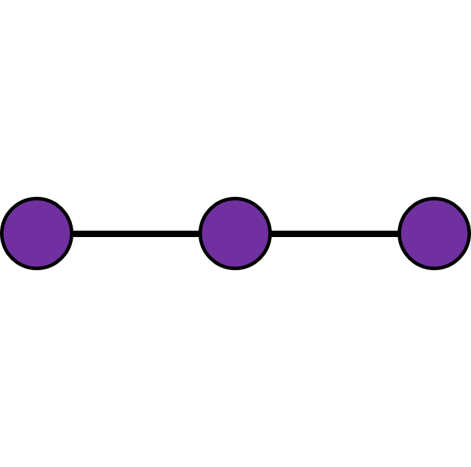
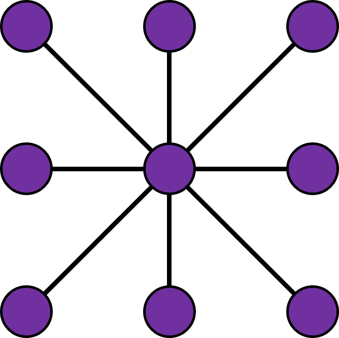
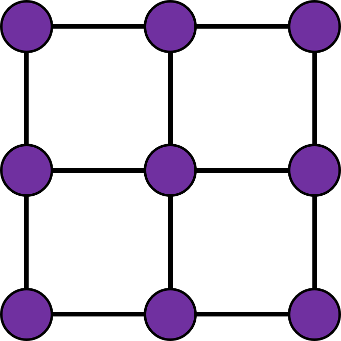
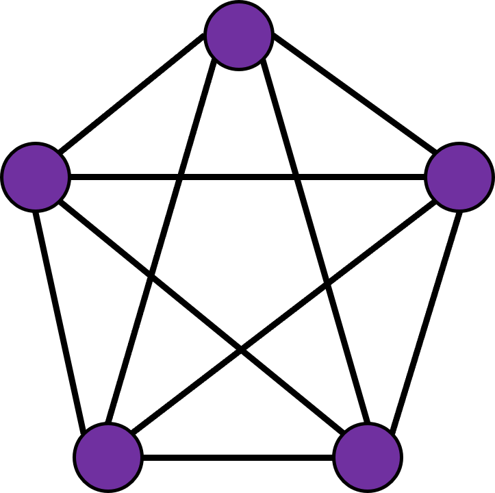
In this section we perform numerical simulations to validate our theoretical results. We consider $4$ different types of graph that can be easily generated with an arbitrary number of nodes $p$. In 1(a) and 1(b) we depict two types of trees, a path graph with $p=3$ nodes, and a star graph with $p=9$ nodes, respectively. We will also consider a $\sqrt{p}\times\sqrt{p}$ grid graph (Figure 1(c)), with maximum degree equal to $4$, and the complete graph (1(d)). Since the path and star graphs are trees, they have $p-1$ edges. The $\sqrt{p}\times\sqrt{p}$ grid graph has $2\sqrt{p}(\sqrt{p}-1)$ edges. The complete graph has $p(p-1)/2$ edges. For the path, star and complete graphs we set $p\in\{100,225,375,500\}$, and for the grid graph we set $p\in\{100,225,361,484\}$, since we require $\sqrt{p}$ to be integer. All graphs have edge weights $w^{\star}_{e}=1$.

For each graph type and dimension $p$, we construct the CGL matrix ${\bf L}^{\star}$, and generate $T=100$ data matrices ${\bf X}$ of size $p\times 500$, with i.i.d. Gaussian columns, zero mean and covariance matrix $({\bf L}^{\star})^{\dagger}$.

6.1 Estimation without topology constraints

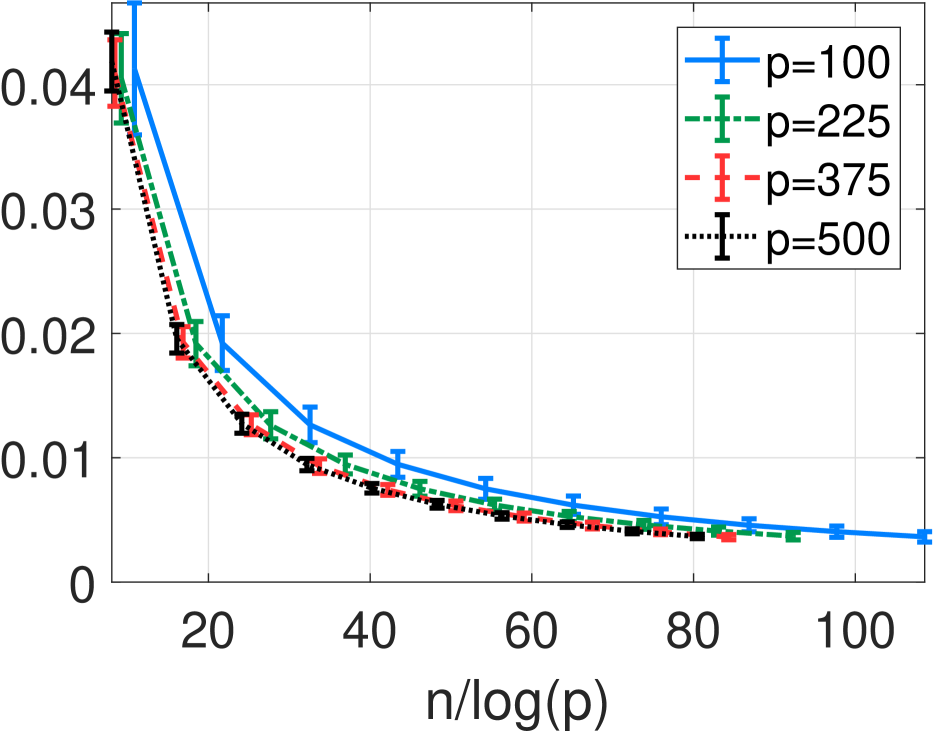
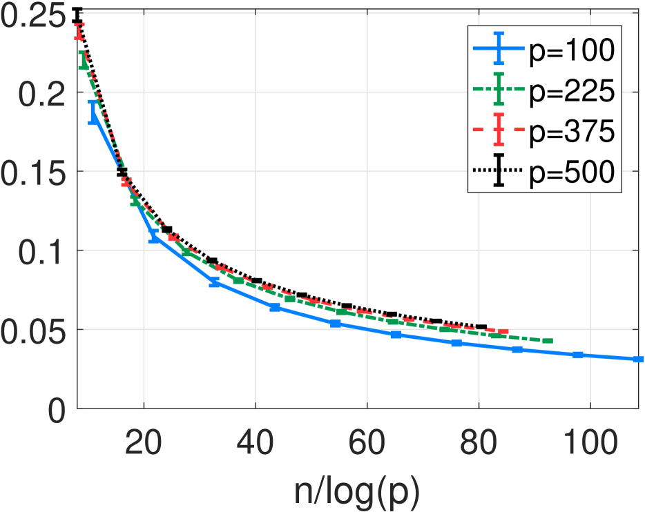
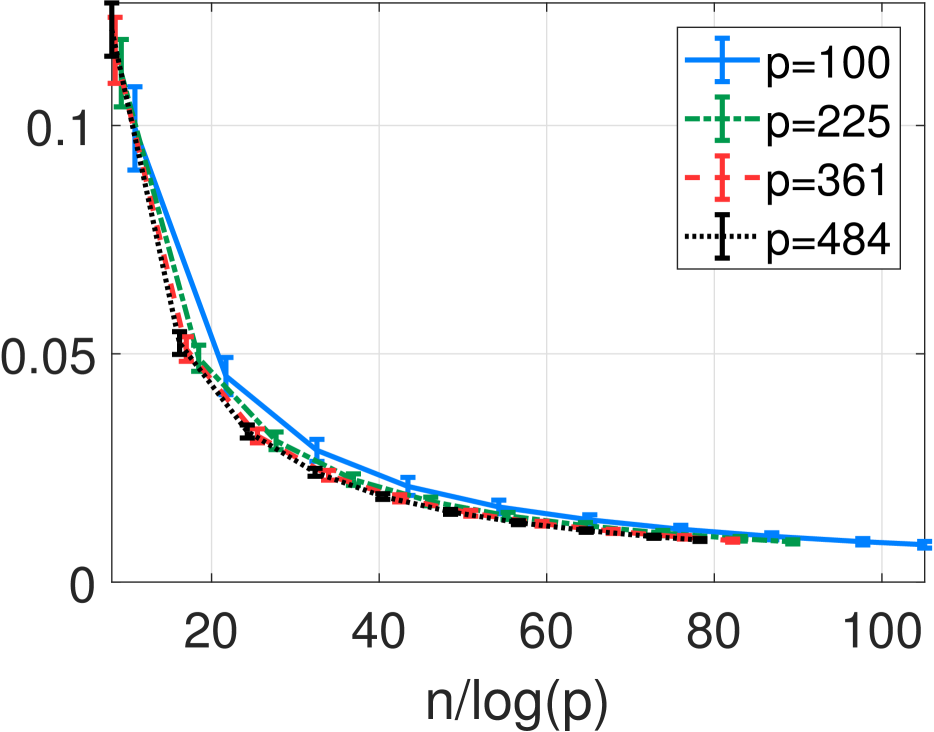
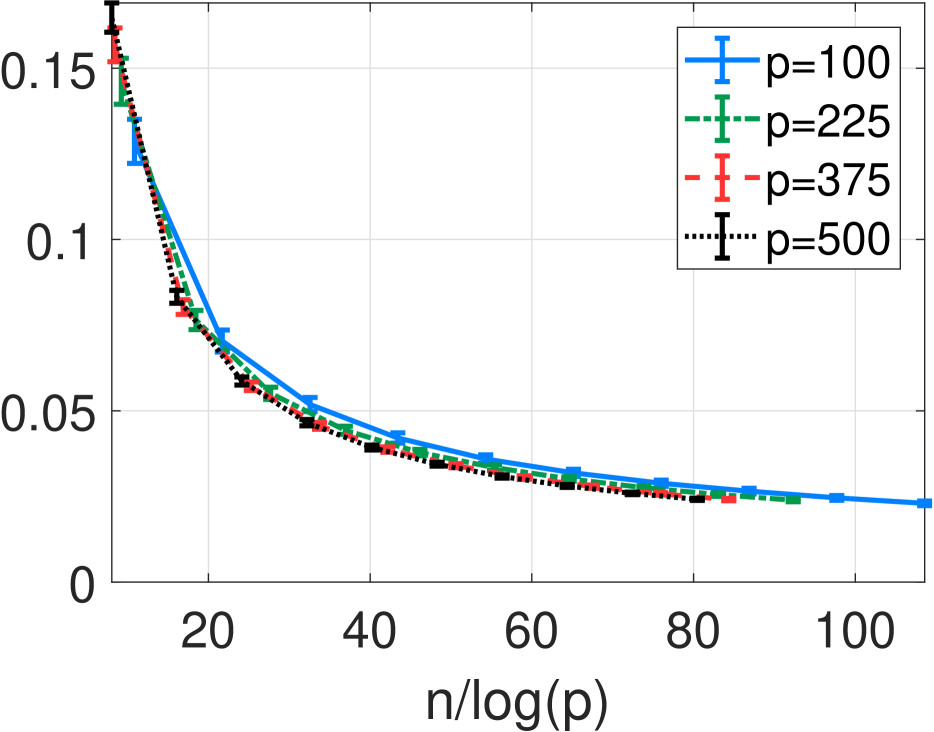
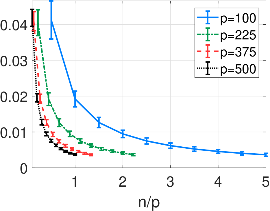
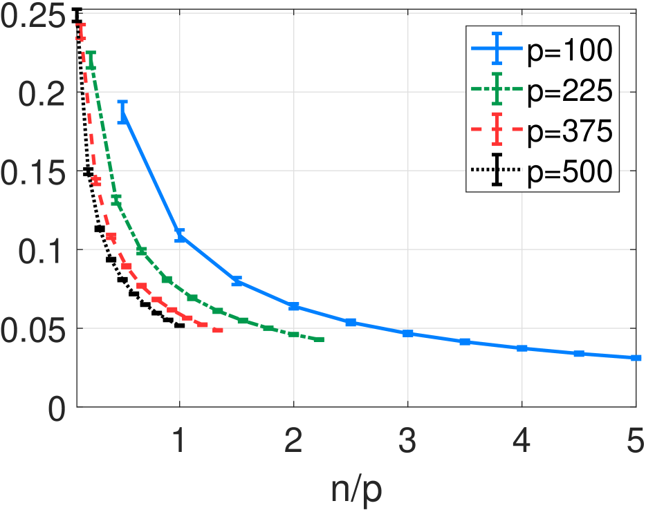
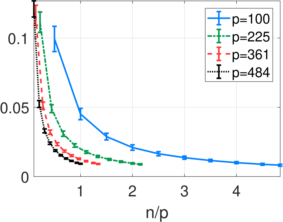
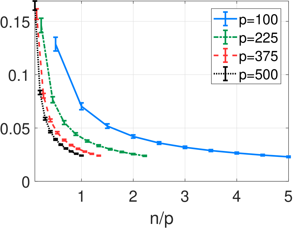
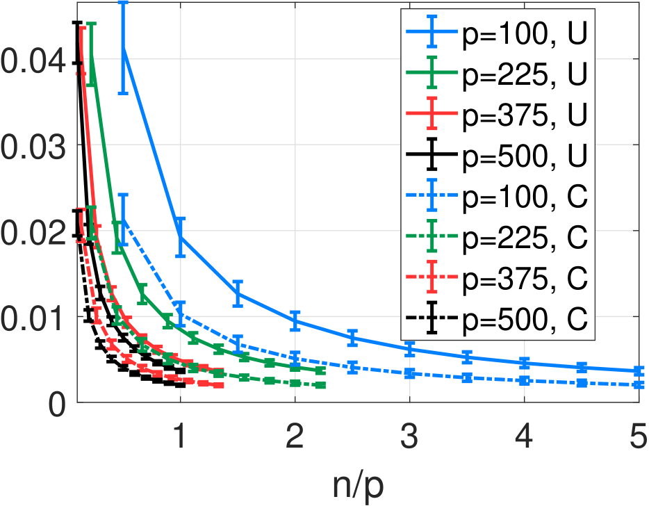
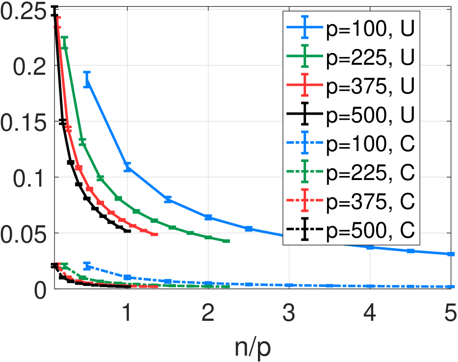
First we evaluate the performance of the CGLE when the constraint edge set is the complete graph, hence, there is no prior information about the true graph topology. We take several values of of $n\in[50,500]$, compute the sample covariance matrix and calculate the CGLE using the coordinate descent algorithm proposed by Pavez and Ortega (2019)(https://github.com/STAC-USC/graph_learning_CombLap), using their default parameters. For each graph, and pair $(p,n)$ we repeat the experiment $T$ times. In Figure 2 we show the average values of $L^{ss}$, with error bars of $1$ standard deviation, as a function of $n/\log(p)$. Note that for each graph type, all curves clump together, in agreement with the weak dependence on the dimension predicted by Theorem 3. In Figure 3, we show the same data as in Figure 2, but now as a function of $n/p$. We observe that for all graph types, and for each value of $n/p$, the symmetrized Stein loss approaches zero faster in higher dimensions, as predicted in (20).

6.2 Estimation with topology constraints

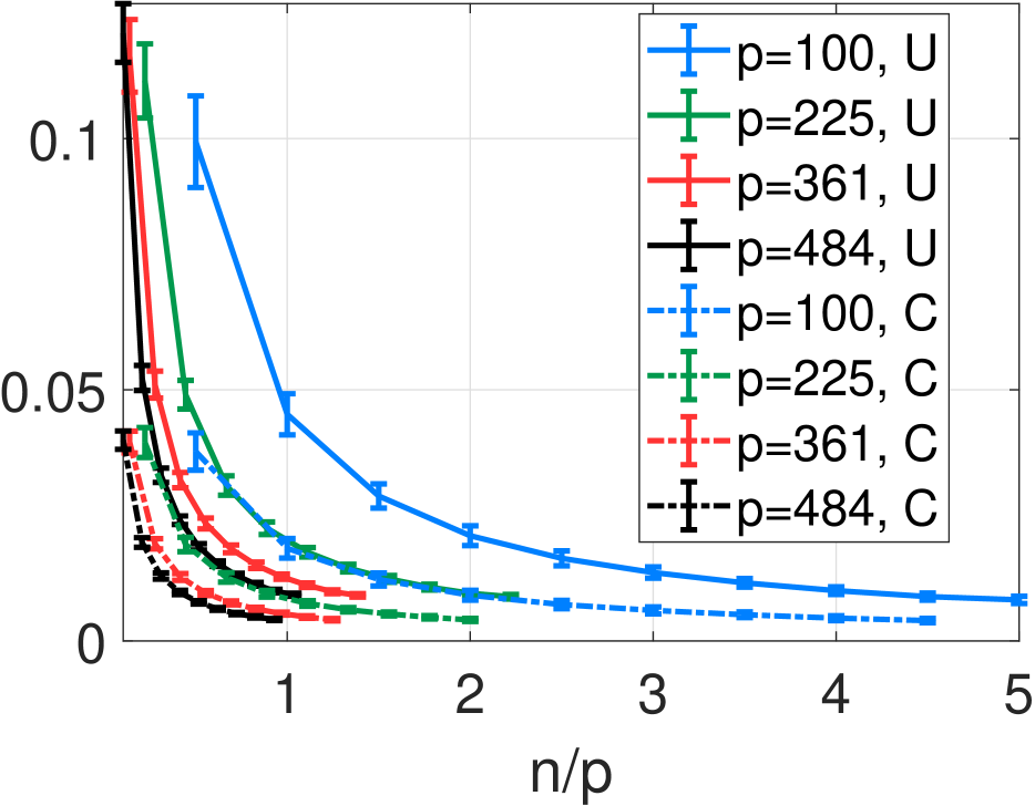
We compare the CGLE with and without knowledge of the true graph topology ${\cal E}^{\star}$. We only consider the sparse graphs (path, star and grid). Figure 4 displays the symmetrized Stein loss as a function of $n/p$. For all graphs, and all pairs $(n,p)$, graph structure constraints reduces the loss. In the unconstrained case (solid lines in Figure 4), the star graph has the highest loss, and takes longer to converge, while the path graph is the fastest. Once the tree constraint is added, the path and star graphs have similar fast convergence behavior. This similitude may be attributed to the values taken by the effective resistances of edges and non edges. For the path, $r^{\star}_{e}=1$ for edges, while is takes values between $2$ and $p-1$ for non edges. For the grid graph, the edge effective resistances are smaller than $1$, while the non edge resistances can be much larger. For the star graph, the edge resistances are equal to $1$, while all the non edge resistances are equal to $2$. When $n$ is smaller, it is more likely that a edge and non edge resistances are similar for the star graph, than for the path and grid graphs, resulting more difficult to obtain an accurate estimation of the CGL, and distinguish between edges and non edges.

7 Conclusion

In this paper we proved that the combinatorial graph Laplacian estimator with edge constraints exists, if and only if, a certain data dependent graph is connected. We proposed the symmetrized Stein loss for CGL matrices of connected graphs. We showed that the CGLE is consistent under this loss, even in high dimensions. Unlike previous consistency results for various graph Laplacian estimators, our proof does not require (non) convex regularization, sparsity, or other type of structure. For tree structured graphs, when the graph topology is known, we can achieve consistency at a faster rate. Interesting directions for future work include improvements to the error bounds that exploit the graph structure to narrow the gap between the convergence rates from Theorem 3 and Theorem 4, analysis of other estimators for the CGL using the symmetrized Stein loss, and determining optimal convergence rates and matching lower bounds.

Acknowledgements

The author thanks Antonio Ortega for useful discussions. This work was funded by NSF under grants CCF-1410009 and CCF-2009032.

 

Supplementary Material:
Laplacian Constrained Precision Matrix Estimation: Existence and High Dimensional Consistency

 

Appendix A Bounds on edge weights of GGLE

Consider the GGL estimation problem, with $\alpha\geq 0$

$$\min_{\Theta_{ij}\leq 0,i\neq j}-\log{\hbox{det}}(\hbox{\boldmath$\Theta$})+\operatorname*{tr}(\hbox{\boldmath$\Theta$}{\bf S})+\alpha\sum_{i\neq j}|\Theta_{ij}|.$$ (36)

Let ${\bf K}={\bf S}+\alpha({\bf I}-\mathbf{1}\mathbf{1}^{\top})$, and $\hbox{\boldmath$\Lambda$}=(\lambda_{ij})$ with $\lambda_{ii}=0$ for all $i$. The KKT optimality conditions are

$$-\hbox{\boldmath$\Theta$}^{-1}+\mathbf{K}+\mathbf{\Lambda} =0$$ (37)

$$\lambda_{ij}\Theta_{ij} =0,~{}\forall i\neq j$$ (38)

$$\Theta_{ij} \leq 0,~{}\forall i\neq j$$ (39)

$$\lambda_{ij} \geq 0,~{}\forall i\neq j$$ (40)

$$\Theta \succ 0.$$ (41)

Consider the set ${\cal S}=\{i,j\}$. We can rewrite (37) for the sub-matrices indexed by ${\cal S}$, thus

$$(\hbox{\boldmath$\Theta$}^{-1})_{{\cal S},{\cal S}}={\bf K}_{{\cal S},{\cal S}}+\hbox{\boldmath$\Lambda$}_{{\cal S},{\cal S}}.$$ (42)

Using the Schur complement we have that

$$\hbox{\boldmath$\Theta$}_{{\cal S},{\cal S}}-\hbox{\boldmath$\Theta$}_{{\cal S},{\cal S}^{c}}(\hbox{\boldmath$\Theta$}_{{\cal S}^{c},{\cal S}^{c}})^{-1}\hbox{\boldmath$\Theta$}_{{\cal S}^{c},{\cal S}}=({\bf K}_{{\cal S},{\cal S}}+\hbox{\boldmath$\Lambda$}_{{\cal S},{\cal S}})^{-1}.$$ (43)

Since $\hbox{\boldmath$\Theta$}_{{\cal S}^{c},{\cal S}^{c}}$ is a GGL matrix, its inverse is non negative, thus the matrix $\hbox{\boldmath$\Theta$}_{{\cal S},{\cal S}^{c}}(\hbox{\boldmath$\Theta$}_{{\cal S}^{c},{\cal S}^{c}})^{-1}\hbox{\boldmath$\Theta$}_{{\cal S}^{c},{\cal S}}$ is also non negative (entrywise), and

$$\hbox{\boldmath$\Theta$}_{{\cal S},{\cal S}}\geq({\bf K}_{{\cal S},{\cal S}}+\hbox{\boldmath$\Lambda$}_{{\cal S},{\cal S}})^{-1}.$$ (44)

Since ${\bf K}_{{\cal S},{\cal S}}+\hbox{\boldmath$\Lambda$}_{{\cal S},{\cal S}}$ is a $2\times 2$ matrix, we can compute its inverse in closed form, leading to the inequality

$$\Theta_{ij}\geq\frac{-(K_{ij}+\lambda_{ij})}{K_{ii}K_{jj}-(K_{ij}+\lambda_{ij})^{2}}.$$ (45)

When $\Theta_{ij}<0$, we have that $\lambda_{ij}=0$, and $K_{ij}\geq 0$, thus

$$|\Theta_{ij}|\leq\frac{K_{ij}}{K_{ii}K_{jj}-K_{ij}^{2}}.$$ (46)

The inequality of Table 1 follows after taking $\alpha=0$ and normalizing by $S_{ii}S_{jj}$.

Appendix B Auxiliary lemmas

Lemma 1.

Let each column of ${\bf X}$ be independent identically distributed, and satisfying Assumption 1, then for all $t>0$,

$$\operatorname*{\mathbb{P}}(\Delta({\cal E})>C(t+\sqrt{2t}))\leq 2|{\cal E}|\exp(-nt),$$ (47)

For some universal constant $C$ depending on Assumption 1.

Proof.

We write ${\bf g}_{e}^{\top}(\hbox{\boldmath$\Sigma$}^{\star}-{\bf S}){\bf g}_{e}=r_{e}^{\star}-h_{e}$, and apply Lemma 6 from Jankova and Van De Geer (2015), then for all $t>0$

$$\operatorname*{\mathbb{P}}(|{\bf g}_{e}^{\top}({\bf S}-\hbox{\boldmath$\Sigma$}^{\star}){\bf g}_{e}|>Cr_{e}^{\star}(t+\sqrt{2t}))\leq 2\exp(-nt).$$ (48)

We conclude by taking an union bound. ∎

Lemma 2.

Under the assumptions of Lemma 1, fix $\epsilon>0$, if

$$n\geq(16C^{2}\epsilon^{-2}\vee 1)2\log(p)$$ (49)

then $\Delta({\cal E})\leq\epsilon$ with probability at least $1-2p^{-2}$.

Proof.

Set $t=4\log(p)/n$, and since $|{\cal E}|\leq p^{2}$, from Lemma 1 we have that

$$\Delta({\cal E})\leq 2C\left(\frac{2\log(p)}{n}+\sqrt{\frac{2\log(p)}{n}}\right),$$ (50)

with probability at least $1-2p^{-2}$. We need to pick $n$, so that the RHS of (50) is below $\epsilon$. First note that since $n\geq 2\log(p)$, then the RHS of (50) obeys

$$\Delta({\cal E})\leq 4C\sqrt{\frac{2\log(p)}{n}}.$$ (51)

The desired claim follows since $n\geq 32C^{2}\epsilon^{-2}\log(p)$. ∎

Appendix C Proof of Theorem 4

$$L^{ss}(\widehat{{\bf L}},{\bf L}^{\star}) \leq\frac{\Delta({\cal E})^{2}}{2(p-1)}\sum_{e\in{\cal E}}\hat{w}_{e}r_{e}^{\star}\leq\Delta({\cal E})^{2}(1+L^{ss}(\widehat{{\bf L}},{\bf L}^{\star})).$$ (52)

The last display uses the relation $\sum_{e\in{\cal E}}\hat{w}_{e}r_{e}^{\star}=\operatorname*{tr}(\widehat{{\bf L}}\hbox{\boldmath$\Sigma$}^{\star})\leq 2(p-1)(1+L^{ss}(\widehat{{\bf L}},{\bf L}^{\star}))$, as in the proof of Theorem 3. We can use Lemma 1, and since the graph is a tree, ${\cal E}\leq p$, thus

$$\operatorname*{\mathbb{P}}(\Delta({\cal E})>C(t+\sqrt{2t}))\leq 2p\exp(-nt).$$ (53)

If we pick $t=3\log(p)/n$, we have that with probability at least $1-2/p^{2}$,

$$\Delta({\cal E})\leq C\left(\frac{3\log(p)}{n}+\sqrt{\frac{6\log(p)}{n}}\right).$$ (54)

Now for any $\epsilon>0$, if $n\geq 3(8C^{2}\epsilon^{-1}\vee 1)\log(p)$, then with probability greater than $1-2/p^{2}$

$$\Delta({\cal E})\leq 2C\sqrt{\frac{6\log(p)}{n}}\leq\epsilon.$$ (55)

Now picking $\epsilon^{2}=1/2$, from (52) we obtain

$$L^{ss}(\widehat{{\bf L}},{\bf L}^{\star})\leq 2\Delta({\cal E})^{2}\leq 48C^{2}\frac{\log(p)}{n}.$$ (56)

References

- Agrawal et al. (2019) R. Agrawal, U. Roy, and C. Uhler. Covariance matrix estimation under total positivity for portfolio selection. arXiv preprint arXiv:1909.04222, 2019.
- Bronstein et al. (2017) M. M. Bronstein, J. Bruna, Y. LeCun, A. Szlam, and P. Vandergheynst. Geometric deep learning: going beyond euclidean data. IEEE Signal Processing Magazine, 34(4):18–42, 2017.
- Bunea and Xiao (2015) F. Bunea and L. Xiao. On the sample covariance matrix estimator of reduced effective rank population matrices, with applications to fpca. Bernoulli, 21(2):1200–1230, 2015.
- Cai et al. (2011) T. Cai, W. Liu, and X. Luo. A constrained l1 minimization approach to sparse precision matrix estimation. Journal of the American Statistical Association, 106(494):594–607, 2011.
- Cai et al. (2016) T. T. Cai, Z. Ren, and H. H. Zhou. Estimating structured high-dimensional covariance and precision matrices: Optimal rates and adaptive estimation. Electronic Journal of Statistics, 10(1):1–59, 2016.
- Dempster (1972) A. P. Dempster. Covariance selection. Biometrics, pages 157–175, 1972.
- Dong et al. (2019) X. Dong, D. Thanou, M. Rabbat, and P. Frossard. Learning graphs from data: A signal representation perspective. IEEE Signal Processing Magazine, 36(3):44–63, 2019.
- Dong et al. (2020) X. Dong, D. Thanou, L. Toni, M. Bronstein, and P. Frossard. Graph signal processing for machine learning: A review and new perspectives. IEEE Signal Processing Magazine, 37(6):117–127, 2020.
- Egilmez et al. (2017) H. E. Egilmez, E. Pavez, and A. Ortega. Graph learning from data under laplacian and structural constraints. IEEE Journal of Selected Topics in Signal Processing, 11(6):825–841, 2017.
- Egilmez et al. (2018) H. E. Egilmez, E. Pavez, and A. Ortega. Graph learning from filtered signals: Graph system and diffusion kernel identification. IEEE Transactions on Signal and Information Processing over Networks, 5(2):360–374, 2018.
- Ellens et al. (2011) W. Ellens, F. Spieksma, P. Van Mieghem, A. Jamakovic, and R. Kooij. Effective graph resistance. Linear algebra and its applications, 435(10):2491–2506, 2011.
- Fiedler (1973) M. Fiedler. Algebraic connectivity of graphs. Czechoslovak mathematical journal, 23(2):298–305, 1973.
- Friedman et al. (2008) J. Friedman, T. Hastie, and R. Tibshirani. Sparse inverse covariance estimation with the graphical lasso. Biostatistics, 9(3):432–441, 2008.
- Hassan-Moghaddam et al. (2016) S. Hassan-Moghaddam, N. K. Dhingra, and M. R. Jovanović. Topology identification of undirected consensus networks via sparse inverse covariance estimation. In Decision and Control (CDC), 2016 IEEE 55th Conference on, pages 4624–4629. IEEE, 2016.
- Hsieh et al. (2012) C.-J. Hsieh, A. Banerjee, I. Dhillon, and P. Ravikumar. A divide-and-conquer method for sparse inverse covariance estimation. Advances in Neural Information Processing Systems, 25:2330–2338, 2012.
- Hu et al. (2021) W. Hu, J. Pang, X. Liu, D. Tian, C.-W. Lin, and A. Vetro. Graph signal processing for geometric data and beyond: Theory and applications. IEEE Transactions on Multimedia, 2021.
- Jankova and Van De Geer (2015) J. Jankova and S. Van De Geer. Confidence intervals for high-dimensional inverse covariance estimation. Electronic Journal of Statistics, 9(1):1205–1229, 2015.
- Klein and Randić (1993) D. J. Klein and M. Randić. Resistance distance. Journal of mathematical chemistry, 12(1):81–95, 1993.
- Koyakumaru et al. (2021) T. Koyakumaru, M. Yukawa, E. Pavez, and A. Ortega. A graph learning algorithm based on gaussian markov random fields and minimax concave penalty. In ICASSP 2021-2021 IEEE International Conference on Acoustics, Speech and Signal Processing (ICASSP), pages 5410–5414. IEEE, 2021.
- Kumar et al. (2020) S. Kumar, J. Ying, J. d. M. Cardoso, and D. P. Palomar. A unified framework for structured graph learning via spectral constraints. Journal of Machine Learning Research, 21(22):1–60, 2020.
- Lake and Tenenbaum (2010) B. Lake and J. Tenenbaum. Discovering structure by learning sparse graphs. In Proceedings of the 32nd Annual Conference of the Cognitive Science Society, 2010.
- Lauritzen et al. (2019) S. Lauritzen, C. Uhler, and P. Zwiernik. Maximum likelihood estimation in gaussian models under total positivity. The Annals of Statistics, 47(4):1835–1863, 2019.
- Lauritzen (1996) S. L. Lauritzen. Graphical models, volume 17. Clarendon Press, 1996.
- Ledoit and Wolf (2018) O. Ledoit and M. Wolf. Optimal estimation of a large-dimensional covariance matrix under stein’s loss. Bernoulli, 24(4B):3791–3832, 2018.
- Lounici (2014) K. Lounici. High-dimensional covariance matrix estimation with missing observations. Bernoulli, 20(3):1029–1058, 2014.
- Lu et al. (2018) K.-S. Lu, E. Pavez, and A. Ortega. On learning laplacians of tree structured graphs. In 2018 IEEE Data Science Workshop (DSW), pages 205–209. IEEE, 2018.
- Mateos et al. (2019) G. Mateos, S. Segarra, A. G. Marques, and A. Ribeiro. Connecting the dots: Identifying network structure via graph signal processing. IEEE Signal Processing Magazine, 36(3):16–43, 2019.
- Mazumder and Hastie (2012) R. Mazumder and T. Hastie. Exact covariance thresholding into connected components for large-scale graphical lasso. The Journal of Machine Learning Research, 13(1):781–794, 2012.
- Moghaddam and Jovanovic (2017) S. H. Moghaddam and M. R. Jovanovic. Topology design for stochastically-forced consensus networks. IEEE Transactions on Control of Network Systems, 2017.
- Ortega (2022) A. Ortega. Introduction to Graph Signal Processing. Cambridge University Press, 2022.
- Ortega et al. (2018) A. Ortega, P. Frossard, J. Kovačević, J. M. Moura, and P. Vandergheynst. Graph signal processing: Overview, challenges, and applications. Proceedings of the IEEE, 106(5):808–828, 2018.
- Pavez and Ortega (2019) E. Pavez and A. Ortega. An efficient algorithm for graph laplacian optimization based on effective resistances. In 2019 53rd Asilomar Conference on Signals, Systems, and Computers, pages 51–55. IEEE, 2019.
- Pavez et al. (2018) E. Pavez, H. E. Egilmez, and A. Ortega. Learning graphs with monotone topology properties and multiple connected components. IEEE Transactions on Signal Processing, 66(9):2399–2413, 2018.
- Rabbat (2017) M. G. Rabbat. Inferring sparse graphs from smooth signals with theoretical guarantees. In 2017 IEEE International Conference on Acoustics, Speech and Signal Processing (ICASSP), pages 6533–6537. IEEE, 2017.
- Rothman et al. (2008) A. J. Rothman, P. J. Bickel, E. Levina, and J. Zhu. Sparse permutation invariant covariance estimation. Electronic Journal of Statistics, 2:494–515, 2008.
- Shuman et al. (2013) D. I. Shuman, S. K. Narang, P. Frossard, A. Ortega, and P. Vandergheynst. The emerging field of signal processing on graphs: Extending high-dimensional data analysis to networks and other irregular domains. IEEE signal processing magazine, 30(3):83–98, 2013.
- Slawski and Hein (2015) M. Slawski and M. Hein. Estimation of positive definite m-matrices and structure learning for attractive gaussian markov random fields. Linear Algebra and its Applications, 473:145–179, 2015.
- Soloff et al. (2020) J. A. Soloff, A. Guntuboyina, and M. I. Jordan. Covariance estimation with nonnegative partial correlations. arXiv preprint arXiv:2007.15252, 2020.
- Stein (1975) C. Stein. Estimation of a covariance matrix. In 39th Annual Meeting IMS, Atlanta, GA, 1975, 1975.
- Tugnait (2021) J. K. Tugnait. Sparse graph learning under laplacian-related constraints. IEEE Access, 9:151067–151079, 2021.
- Uhler (2012) C. Uhler. Geometry of maximum likelihood estimation in gaussian graphical models. The Annals of Statistics, 40(1):238–261, 2012.
- Vershynin (2018) R. Vershynin. High-dimensional probability: An introduction with applications in data science, volume 47. Cambridge university press, 2018.
- Von Luxburg (2007) U. Von Luxburg. A tutorial on spectral clustering. Statistics and computing, 17(4):395–416, 2007.
- Witten et al. (2011) D. M. Witten, J. H. Friedman, and N. Simon. New insights and faster computations for the graphical lasso. Journal of Computational and Graphical Statistics, 20(4):892–900, 2011.
- Xiao and Gutman (2003) W. Xiao and I. Gutman. Resistance distance and laplacian spectrum. Theoretical chemistry accounts, 110(4):284–289, 2003.
- Ying et al. (2020) J. Ying, J. V. de Miranda Cardoso, and D. Palomar. Nonconvex sparse graph learning under laplacian constrained graphical model. Advances in Neural Information Processing Systems, 33, 2020.
- Ying et al. (2021) J. Ying, J. M. Cardoso, and D. Palomar. Minimax estimation of laplacian constrained precision matrices. In International Conference on Artificial Intelligence and Statistics, pages 3736–3744. PMLR, 2021.
- Zhang et al. (2020) Y. Zhang, K.-C. Toh, and D. Sun. Learning graph laplacian with mcp. arXiv preprint arXiv:2010.11559, 2020.
- Zhao et al. (2019) L. Zhao, Y. Wang, S. Kumar, and D. P. Palomar. Optimization algorithms for graph laplacian estimation via admm and mm. IEEE Transactions on Signal Processing, 67(16):4231–4244, 2019.