RRFT: A Rank-Based Resource Aware Fault Tolerant Strategy for Cloud Platforms

Abstract

The applications that are deployed in the cloud to provide services to the users encompass a large number of interconnected dependent cloud components. Multiple identical components are scheduled to run concurrently in order to handle unexpected failures and provide uninterrupted service to the end user, which introduces resource overhead problem for the cloud service provider. Furthermore such resource-intensive fault tolerant strategies bring extra monetary overhead to the cloud service provider and eventually to the cloud users. In order to address these issues, a novel fault tolerant strategy based on the significance level of each component is developed. The communication topology among the application components, their historical performance, failure rate, failure impact on other components, dependencies among them, etc., are used to rank those application components to further decide on the importance of one component over others. Based on the rank, a Markov Decision Process (MDP) model is presented to determine the number of replicas that varies from one component to another. A rigorous performance evaluation is carried out using some of the most common practically useful metrics such as, recovery time upon a fault, average number of components needed, number of parallel components successfully executed, etc., to quote a few, with similar component ranking and fault tolerant strategies. Simulation results demonstrate that the proposed algorithm reduces the required number of virtual and physical machines by approximately 10% and 4.2%, respectively, compared to other similar algorithms.

1 Introduction

Huge amount of physical servers connected through very high network bandwidth is the backbone of cloud computing environment. The pay-as-you-go model of cloud computing provides the flexibility for users to access physical servers on rented basis from cloud service provider (CSP). The resources are provided through different service models such Software as a Service (SaaS), Platform as a Service (PaaS), and Infrastructure as a Service (IaaS) [1, 2]. For example, Microsoft Office 365 is implemented in SaaS model to provide the MS office software through the web.

The applications that are specifically designed to deploy in the cloud are referred to as cloud applications. Such applications are accessed remotely through multiple web pages [3]. Network bandwidth plays an important role in providing the software functionalities to the users. In order to simplify the cloud application at the development stage, the entire cloud application is divided into multiple small applications, known as cloud component. A cloud application component is a part of the software package or a module that encapsulates a set of interrelated functions or tasks. For example, in document editing cloud applications, the module that is responsible for saving and exporting the document in a specific format can be considered as one cloud component. Each cloud component receives a set of inputs and executes a set of predefined operations and provides the output to either the user or to other dependent components. In the case of ATM services provided by the banks to its customer, reading the ATM card, communicating the desired remote database, printing the receipt, etc., can be considered as different dependent components.

On the other hand, fault tolerance is becoming an important issue for the cloud research community. The CSP may experience unexpected failure at any time while providing the service through efficient scheduling mechanisms [4]. A fault may occur at the hardware level due to a power outage or at the software level [5], which may occur due to the ambiguous input to the cloud application. Different mechanisms have been proposed in recent years to prevent and handle the pre-failure and post-failure situations. Authors in [6] present an extensive survey on fault tolerant architectures in cloud computing.

Different fault tolerant mechanisms that are available in the research community are recovery block, N-version programming, parallel, and VM-restart [7]. In order to prevent unexpected failure, the applications are executed on multiple cloud servers. In the recovery block fault tolerant mechanism, applications are executed sequentially for a certain number of time until the desired output is obtained. In contrast, the application is scheduled to execute on multiple cloud servers concurrently in parallel fault tolerant strategy until the first output is obtained [8]. Taking software bugs into consideration, multiple equivalent applications are scheduled to run concurrently on multiple cloud servers. All outputs are then compared and the most similar output is provided to the user. As the failure may occur at the virtual machine or cloud servers level, restarting the virtual machine itself is one of the most popular and simple fault tolerant strategies. In fault tolerance strategies, a large number of resources are wasted, where multiple VMs are engaged for a single component, especially for long-running jobs [9]. Among all fault tolerant strategies, the time required to finish execution of the cloud application and the amount of resource required are inversely proportional to each other. In recovery block fault tolerant strategy, the time required to finish the execution of application successfully is more than that of the parallel fault tolerant strategy and vice-versa.

Efficient fault tolerant strategies are mainly either time-driven or resource-driven. In case of time-driven strategies, the applications are executed multiple times until the required result is obtained. However, in the case of resource-driven, multiple identical applications or similar applications are executed by allocating more resources. Based on the critical level of the application, the CSP needs to provide sufficient amount of resource or time. If the application is time-constrained, CSP needs to provide more resource for parallel execution of the identical applications and ensure that the application is finished on time. However, if the application is cost-constrained, the CSP provide minimum but sufficient amount of memory to the application to execute and obtain the result. In such cases, the CSP executes the applications only upon failure. However, in the former case, irrespective of the correctness of the result, the CSP needs to allocate more than the required amount of memory.

In the current research era, a huge number of complex, time-consuming algorithms are designed to carry out specific operations such as DNA sequencing in bioinformatics involve very complex algorithms. As the current research is heading toward simplifying the human life, the cloud applications are becoming more complex and large in terms of the number of cloud components involved in the corresponding applications. Components that are involved in one cloud application are interconnected and dependent on each other. Despite numerous advantages provided by the cloud platforms, CSPs experience unexpected failures in providing the services, which are the major research issues. By connecting the unexpected failure issues to a large number of complex inter-dependent cloud components, it is observed that a single failure of any cloud component may lead to the failure of the entire cloud application [10]. Failure of cloud applications has a great impact on QoS which affects the decision to take the cloud service from a particular CSP [3]. On the other hand, providing service with a higher degree of fault tolerance is a resource-intensive job for cloud service providers, which further introduces extra monetary overhead to the CSP and eventually to the cloud users.

1.1 Motivation

The large cloud applications are mainly consisting of a large number of interconnected components, where each component is responsible for providing separate functionality. However, the user may experience interruption due to unexpected error or fault in the cloud application during service period, which incurs huge monetary cost to the cloud user as well as to the cloud service provider.

Cloud application may encounter faults due to several reasons such as software bugs, erroneous input data, hardware failures, etc. A fault may bring down the whole cloud application or multiple components. For example, failure of the components that pre-process the incoming raw CCTV footage could hamper the whole real-time security system in a cloud-based smart city solution. On the other hand, some components are responsible for sending the processed and compressed CCTV footage to the storage servers for the backup purpose. Failure of such components would not affect the real-time security system. This paper mainly considers such cloud applications. In general, at any particular time, a subset of components is active providing services to the users. It is assumed that components are associated with different priorities based on the functionalities. Applying fault tolerant mechanisms to the whole cloud application or all components without considering the functionality of each component could be resource-intensive job and therefore would be expensive.

The faults are handled by mainly two kinds of strategies: replication and re-execution. In the replication strategy, multiple identical components are scheduled to run concurrently, which is a resource-intensive strategy. In the re-execution strategy, the same component is executed again only if the component failed while providing the services. This strategy eliminates the additional resource demand. However, this introduces additional time as the component may need to start from either the beginning or from the last saved restore point.

Besides, the problem of providing a huge amount of resources to the cloud application, the placement of the backup component plays a vital role in providing an efficient fault tolerance strategy. Primary components communicate among each other while providing the service to the user. Furthermore, to provide uninterrupted service by tolerating a higher degree of faults, primary components communicate with their backup components in case of a replication strategy. Upon failure of the primary component, one of the backup components will act as the new primary component and interact with other primary components. The network latency between the primary and the backup component may affect the QoS, which infers the importance of placement of both components. Here, placement of the component refers to the selection of a physical machine for deploying the component. It is essential to consider the communication or the placement of the backup components as a major factor while designing the fault tolerant strategy. Further, it is also not recommended to apply the re-execution strategy onto all the components in order to save the resources and minimize the service cost, as this would incur higher degradation of service quality. The aforementioned scenarios of providing efficient fault tolerant service by reducing the total amount of required resource without compromising the service quality and placement of component onto suitable PM motivates us to propose an efficient fault tolerant mechanism.

As it is clearly mentioned in Section 1.1, providing fault tolerant service to cloud application that consists of a very large number of cloud components is resource-intensive, in this paper, we attempt to propose a novel resource-aware strategy that provides fault tolerant services to the significant selective components instead of the whole application. Thus we focus on the design, analysis and evaluation of certain important metrics and experimenting with any real-life application is beyond the scope of this work and serves as an immediate extension, as discussed in Section 7.

The rest of this paper is organized as follows. The related literature survey is presented in Section 2. The concerned problem is formulated in Section 3. The proposed solution that includes the determination of most significant component followed by the fault tolerant algorithm is presented in Section 4. The proposed optimization policy for the total numbers of replicas is presented in Section 5. Performance evaluation and concluding remarks are made in Section 6 and 7, respectively.

2 Related Works

An intensive survey and comparison of the different fault tolerant architectures are presented in [11, 12, 6]. It is emphasized that despite numerous advantage of cloud computing such as reduction of costs, efficient resource utilization [13], leveraging the efficiency and compatibility of software, increasing the storage capacity, etc., immature fault tolerant mechanism plays an important role affecting the decision to adopt cloud computing environment. The survey in [6] classifies the fault tolerance architecture into proactive and reactive architecture. The fault tolerance techniques are applied in different stages of cloud computing, such as in scheduling [14, 15, 16, 17], resource allocation [18, 19], to improve the reliability [20], placement of virtual network function in cloud network [21] etc.

In the scenario of mobile cloud computing, where the entire computation or the part of the computation payload is offloaded to powerful cloud servers, authors in [22] address the offloading problem by taking the portability of mobile device and connectivity issues of the mobile network into consideration. The fault tolerant based offloading mechanism is designed based on the genetic algorithm. Despite numerous advantages of genetic algorithms, the time-consuming process may provide the extra computation overhead to the mobile device, and eventually this may lead to the failure of proposed offloading mechanism. Similar to [10], authors in [23] apply a similar concept to provide fault tolerant service to different component of a cloud application. The rank of a cloud component depends on the reliability properties such as failure rate and failure impact. The fault tolerant strategies are applied to the components based on the reliability, response time, and resource cost. However, it is observed that the component with higher failure rate and failure impact in some component DAG topology are given lower rank value, which contradicts the proposed ranking concept.

Authors in [15] proposed the hybrid task scheduling mechanism offering the fault tolerant service by integrating the tradition backup and checkpoint technology and classifying the tasks and VMs. However, the proposed scheduling strategy allocates the resources among all tasks specifically for the backup purpose without investigating the importance of the tasks. As a result, the resource required is very high in order to implement the proposed scheduling mechanism. Similarly, in [18], the proposed fault tolerant mechanism allocates maximum amount of resource to the tasks, which is a resource-intensive strategy for the cloud service provider. Similarly, authors in [24] formulate the cost-effective fault tolerant strategies in providing services to the multiple tenants in cloud. The major pitfall of the proposed fault tolerant strategy is that the historical behavior of each service is not taken into account, which could have given insight behavior of each service in terms of the failure probabilities.

In order to handle the post-fault events, it is very much essential to detect the fault in every physical server with no delay, as described in [25]. Here, the authors proposed a recovery block’s acceptance test based fault detection scheme for component-based cloud computing environment. The proposed fault detection scheme is dedicated to only software faults, transient hardware faults, and response-time failures. However, the proposed idea does not address the issue of power failure that may cause the failures of the entire server.

Though cloud provider guarantees the resource demand, however, in the data center performance anomalies or failure of expected performance is an upcoming issue, which arises due to sharing of physical resources and multi-tenancy as discussed in [19]. To debug the application failure, distinguishing the faults with global and local impact is essential, as in [19]. Such classifications of faults provide power to the system administrators and the application developer to understand and diagnose the root cause of the failure. Authors in [26], extend the fault classification work as in [19] for automatic fault diagnosis of web applications in cloud computing. Fluctuating workload, management of large-scale application, and modeling the behavior of complex application are some of the major factors that possess greater challenges in fault diagnosis of web applications. The behavior of access patterns is analyzed using correlation analysis, which is used further to detect the faults. However, finding the correlation between the workload and the application may lead to a time-consuming process as the frequency arrival of the application to the cloud service provider is very high.

Authors in [27] proposed fault tolerant enabled storage and processing of data in mobile cloud taking energy consumption as a major parameter into consideration. As running an application needs processing and storage capabilities, authors address the issue of selecting a suitable node that is a mobile device or a cloud, for processing and data storage by following k-out-of-n computing approach. Here, $k$ and $n$ determine the degree of reliability. However, the proposed scheme does not address the issues generated due to the mobility of peer mobile nodes.

Authors in [10] propose the ranking of the cloud components in order to find out the significant component. A cloud application comprises a set of components represented as a directed acyclic graph. The ranking of the cloud component depends on the number of components present in the cloud application and the number of components that invoke the corresponding component. As a cloud application is responsible for providing certain services that are consisting of a large number of components, it is a hectic job to provide the critical status to each component. Further, it is not clear, which component should be given what kind of fault tolerant service.

The major upcoming issue in resource allocation is to distribute the resources among different users with zero faults or higher degrees of fault tolerance, as discussed in [28]. Authors in [28] propose a fault and power-aware reliable resource allocation scheme that emphasizes the failure of request occurs due to fluctuation in power consumption by the requests. However, calculating the power consumption while scheduling both data and compute intensive requests is a cumbersome task.

Handling faults that occur during the execution of real-time tasks in cloud environment requires an efficient fault tolerant mechanism, as demonstrated in [29]. Though the proposed elastic resource provisioning mechanism based on primary-backup model improves the resource utilization in the context of fault tolerant, the faults that occur at the physical server level cannot be handled by the proposed scheduling algorithms. Authors in [30] have proposed similar fault tolerant scientific work-flow scheduling algorithm considering the spot and on-demand instances on the cloud.

3 Problem formulation

Unlike the applications running in conventional personal computers, applications that are deployed in the cloud computing environment and are accessed remotely through the web are known as cloud applications. These applications are often collections of multiple dependent or independent components known as cloud components. In the proposed scenario, each component can either be in an active or inactive state. The active state of a component refers to a state in which the cloud component is engaged in providing services to the cloud user directly or indirectly, which is inactive otherwise. At any given time $t$, a component is said to be an active component if the same component is in the active state. Let, $n$ number of active components from a total of $N$ number of components, the relationship between $n$ and $N$ can be written as $1\leq n\leq N$.

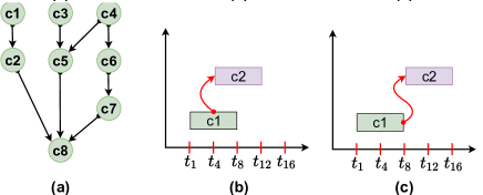
A component is said to be dependent if it requires the output or the intermediate result of another component. A Directed Acyclic Graph (DAG) is used as a mathematical tool to represent the dependencies among the active components. One vertex in the DAG represents one active component. An edge represents the dependency of one component over another one. For example, Figure 1(a) shows the dependencies of eight components, where component $c2$ depends on the output of the intermediate results of the component $c1$, and $c5$ requires the output or intermediate results of component $c3$ and $c4$ and so on.

Based on the dependencies, a dependent component cannot start its execution before the execution of the preceding component. Figure 1(b) and 1(c) illustrate this situation. In Figure 1(b), component $c2$ may start its execution after receiving the intermediate result from component $c1$, whereas, in Figure 1(c), component $c2$ starts its execution after receiving the final output from component $c1$. However, it is assumed that a dependent component may finish its execution before or after the execution of the preceding component. As shown in Figure 1, component $c2$ may finish its execution before component $c1$ finishes its execution. It is also assumed that a vertex cannot be isolated. In other words, each component must be connected to at least one other component. Among active components, multiple components can be executed concurrently at any given instant of time. For example, component $c2$, $c5$, and $c6$ can be scheduled to run concurrently as no dependency exists among themselves.

Multiple cloud applications are hosted by cloud service providers, where a vast number of cloud components are involved in providing the service to the cloud users. The cloud application is considered as the input in this research article. Based on the functionality, cloud components are compared and different weights can be assigned to each component in order to calculate their importance level. For example, in ATM withdrawal system, different components are responsible for different operations such as components for cash dispatching, receipt printing, communicating remote database, etc. In such a scenario, the importance level for the component responsible for remote database communication is higher than the component that is responsible for printing the withdrawal receipt. The component with higher importance level, i.e., higher weight is considered as the most significant component. Formally, a component is said to be the most significant cloud component, if it is sufficiently important to be worthy of providing the fault tolerant service. The most significant cloud components are determined programmatically.

In this work, mainly two aspects of fault tolerant services are focused. Firstly, providing an efficient mechanism to rank components thereby determining the most significant cloud components and secondly, apply a fault tolerant mechanism to the cloud components based on their ranks so that the dedicated resources required to provide fault tolerant service can be minimized. Let us take an example to illustrate the latter aspect. Let, $A$, $B$, and $C$ be the three components that are running concurrently with a maximum degree of fault tolerance of $4$. The degree of fault tolerance indicates the number of faults that can be tolerated. We assume that one VM is used to host exactly one component. Considering the number of components and the maximum degree of fault tolerance, we can conclude that a total of $15$ VMs are required to run $A$, $B$, and $C$ and their corresponding replicated components concurrently. Let the importance level of component $A$ be ranked as ”High”, component $B$ be as ”Medium”, and $C$ be ranked as ”Low”. It is this importance of a component that translates to its rank value in our proposed algorithm. With such knowledge regarding the importance of each component and the corresponding failure probability, the resources can be distributed unevenly among all components for fault tolerant service. $6$ VMs can be assigned to component $A$, $4$ VMs can be assigned to component $B$, and $2$ VMs can be assigned to component $C$ for fault tolerant service. As a result, a total of $12$ VMs can be used to provide the fault tolerant service. Further, the degree of fault tolerant can be increased for the components with higher importance level. As discussed in this example, the number of faults of component $A$ that can be tolerated is increased to $6$.

The above example illustrates the goal of this paper, where a fault tolerant strategy needs to be developed that should rank the cloud components and employ a component-specific fault tolerant strategy based on the rank. The following section discussed in detail the procedure to rank the components and the fault tolerant strategy.

Figure 1: An example of DAG

4 The fault tolerant strategy

We believe that providing fault tolerant service to cloud application that consists of huge number of cloud components is resource-intensive and hence inefficient in terms of monetary cost. In order to address this issue, we propose a novel Rank based Resource-aware Fault Tolerant (RRFT) strategy, which provides fault tolerant services to selected significant components instead of the whole application. The proposed RRFT solution has two stages. Firstly, determining the most significant component and secondly, providing the fault tolerant service to each component based on their rank value, which indicates the importance of the component.

4.1 Determination of most significant component

Here, the components of a cloud application are represented as a DAG with no isolated vertex. In other words, at any given time, each component must be connected to at least one other component. We use the group relationship model as a mathematical tool followed by the probabilistic approach in order to find the most significant cloud components of an application. The goal of using group relationship model is to derive the dependency of one active component on all others that belong to the same cloud application. Let, $A$ be the cloud application to which the fault tolerant service needs to be applied. $G=(C,E)$ is the DAG of the set of components $C$ that belongs to cloud application $A$. $E$ represents the dependencies among the components present in $C$. The set $C$ consists of $N$ components, represented by $c_{i},1\leq i\leq N$. Let, $G_{t}^{a}=(C_{t}^{a},E_{t}^{a})$ be the DAG of set of active cloud components $C_{t}^{a}$ and their dependencies $E_{t}^{a}$ of the application $A$ at time $t$. $C_{t}^{a}=\{\hat{c}_{1},\hat{c}_{2},\dots,\hat{c}_{n}\}$ consists of $n$ number of active components. The relation between the sets $C_{t}^{a}$ and $C$ can be written as $C_{t}^{a}\subseteq C$ at any given time $t$.

The DAG $G_{t}^{a}$ can be transformed to the adjacency matrix $\tau_{t}$ as given below.

$$\tau_{t}=[v_{ij}],\quad 1\leq i\leq n,\ 1\leq j\leq n$$ (1)

Where,

$$v_{ij}=\left\{\begin{array}[]{ll}1&\text{if the component }j\text{ depends on component }i;\\ 0&\text{if there is no dependency of component }i\text{ on }j;\\ 0&\text{if }i=j\end{array}\right.$$

The adjacency matrix is derived by looking at the edge set $E_{t}^{a}$ that contains the value ${1,0}$. The adjacency matrix is used to calculate the dependency of component $i$ over component $j$, where, $i\neq j,\forall j\in C_{t}^{a}$. The dependencies that are present in edge set $E_{t}^{a}$ are called one-hop dependency. In order to derive the multi-hop dependencies among components, the distance matrix $\tau_{t}^{d}$ is calculated from the adjacency matrix $\tau_{t}$ as derived below.

$$\tau_{t}^{d}=\begin{bmatrix}d_{11}&d_{12}&\dots&d_{1n}\\ d_{21}&d_{22}&\dots&d_{2n}\\ \vdots&\vdots&\ddots&\vdots\\ d_{n1}&d_{n2}&\dots&d_{nn}\end{bmatrix}$$ (2)

Where,

$$d_{ij}=\left\{\begin{array}[]{ll}d_{ij}&\text{minimum number of intermediate }\\ &\text{components or minimum number of}\\ &\text{ hops from component }i\text{ to }j.\\ 0&\text{If there is no path from component }i\text{ to }j.\\ 0&\text{If }i=j.\end{array}\right.$$ (8)

$$for\quad 1\leq i\leq n,\ 1\leq j\leq n$$

The significant value of an active component $\hat{c}_{j},1\leq j\leq n,$ can be derived by calculating the column sum of distance matrix $\tau_{t}^{d}$. Mathematically,

$$\Psi(\hat{c}_{j})=\sum_{i=1}^{n}{d_{ij}},d_{ij}\in\tau_{t}^{d},1\leq i\leq n,1\leq j\leq n$$ (9)

The component with minimum significant value $\Psi(\hat{c}_{j})$ is considered the most influential component. This is due to the fact that several components depend on the output of such components. For instance, the components $c2,c5,c6,c7,$ and $c8$ depend on the output of the components $c1,c3,$ and $c4$ as shown in Figure 1. Hence, the components $c1,c3,$ and $c4$ could be considered as the most influential components. This indicates that The failure of such component has an impact on a maximum number of other components and therefore has a higher impact on the whole cloud application. The significant value of an active component is further used in the calculation of failure impact of the respective component. The failure impact of one component $F(\hat{c}_{i})$ is calculated as the sum of the significant values of the components $\hat{c}_{j},1\leq j\leq n,i\neq j$ that satisfies the conditions $d_{ij}>0$. Mathematically,

$$F(\hat{c}_{i})=\sum_{j=1}^{n}{\Psi(\hat{c}_{j})},\quad i\neq j,d_{ij}>0,1\leq i\leq n$$ (10)

Along with the failure impact, the historical performance is also taken into account to calculate the accumulated failure impact of a component, $\ddot{F}(\hat{c}_{i})$. The failure rate of a component is represented as $\lambda(\hat{c}_{i}),\forall\hat{c}_{i}\in C_{t}^{a}$. The value of failure rate and failure impact as calculated in Equation 10, is multiplied in order to obtain the value of $\ddot{F}(\hat{c}_{i})$, as in Equation 11.

$$\ddot{F}(\hat{c}_{i})=\lambda(\hat{c}_{i})*F(\hat{c}_{i}),\quad\forall\hat{c}_{i}\in C_{t}^{a}$$ (11)

Furthermore, the information regarding the failure probability $P(\hat{c}_{i})$ of a component $\hat{c}_{i},\forall\hat{c}_{i}\in C_{t}^{a}$ is essential in order to determine the most significant component. It is assumed that the component $\hat{c}_{i}$ will remain active for $h_{i}$ time units and failure of the components follow the Poisson distribution [31]. Considering the aforementioned information, the failure probability of a component can be calculated as follows.

$$P(\hat{c}_{i})=\frac{\lambda(\hat{c}_{i})*h_{i}}{e^{\lambda(\hat{c}_{i})*h_{i}}}$$ (12)

Here, it is assumed that $h_{i}$ is known. However, the average of $h_{i}$ can be taken into account, if the active time duration $h_{i}$ of component $\hat{c}_{i}$ is unknown. The average active time duration can be calculated by taking the ratio of total active time and number of time the component $\hat{c}_{i}$ becomes active from inactive state. Taking the value of accumulated failure impact as given in Equation 11, and failure probability as derived in Equation 12, the most significant value of each component is calculated as derived below.

$$\Omega(\hat{c}_{i})=\ddot{F}(\hat{c}_{i})*P(\hat{c}_{i}),\quad\forall\hat{c}_{i}\in C_{t}^{a}$$ (13)

As the complexity of developing cloud application increases, the complexity of monitoring the behavior of each component’s execution and providing the fault tolerant services also increases. The most significant value of a component is not enough to determine whether the component should be given higher priority while providing the fault tolerant service. The most significant value $\Omega(\hat{c}_{i})$ depends on various factors such as the number of times the component failed over its active time duration, number of dependent components, etc. However, the calculation of $\Omega(\hat{c}_{i})$ does not consider the fact that a single failure of any component may lead to the failure of the whole cloud application.

In order to address this issue, the conventional joint probability distribution approach is applied. The historical information regarding the failure of the cloud application due to failure of a specific component can be obtained from the performance history of each component and the cloud application. Let, $f_{i}$ be the total number of times component $\hat{c}_{i}$ failed. Further, let $f_{i}^{s}$ be the total number of times the whole cloud application is failed due to the failure of component $\hat{c}_{i}$. Using the value of $f_{i}$ and $f_{i}^{s}$, the mean application failure due to the failure of component $\hat{c}_{i}$, $\lambda_{i}^{s}$, can be derived as follows.

$$\lambda_{i}^{s}=\frac{f_{i}^{s}}{f_{i}},\quad 1\leq i\leq n$$ (14)

Using Equation 14 and Equation 12, the cloud application failure probability due to the failure of component $\hat{c}_{i}$, $\ddot{P}(\hat{c}_{i}|A)$ can be derived as

$$\ddot{P}(\hat{c}_{i}|A)=P(\hat{c}_{i})\left[\frac{1}{x!}(\lambda_{i}^{s}h_{i})^{x}e^{-\lambda_{i}^{s}h_{i}}\right]$$ (15)

where, $h_{i}$ is the time duration of the active component $\hat{c}_{i}$. It is assumed that the failure of the components follows Poisson distribution. By putting the value of $x=1$ and the value of $P(\hat{c}_{i})$ in Equation 12, the Equation 15 can be re-written as

$$\ddot{P}(\hat{c}_{i}|A)=\left[\frac{\lambda(\hat{c}_{i})h_{i}}{e^{\lambda(\hat{c}_{i})h_{i}}}\right]*\left[\frac{\lambda_{i}^{s}h_{i}}{e^{\lambda_{i}^{s}h_{i}}}\right]$$

$$=\frac{(h_{i})^{2}\lambda_{i}^{s}\lambda(\hat{c}_{i})}{e^{h_{i}(\lambda(\hat{c}_{i})+\lambda_{i}^{s})}}$$ (16)

$\Omega(\hat{c}_{i})$	$\ddot{P}(\hat{c}_{i}|A)$
$\hat{c}_{2}=0.115$	$\hat{c}_{3}=0.922$
$\hat{c}_{4}=0.0674$	$\hat{c}_{2}=0.617$
$\hat{c}_{1}=0.023$	$\hat{c}_{4}=0.514$
$\hat{c}_{3}=0.008$	$\hat{c}_{1}=0.455$
(a)

Rank ($\beta_{i}$)	Component ($\hat{c}_{i}$)
$\beta_{2}=\beta_{3}=1$	$\hat{c}_{2},\hat{c}_{3}$
$\beta_{4}=2$	$\hat{c}_{4}$
$\beta_{1}=3$	$\hat{c}_{1}$
(b)

TABLE I: An example of ranking the component

Considering the values calculated in Equation 13 and 4.1, components are sorted individually. For the sake of better understanding on how $\Omega(\hat{c}_{i})$ (Equation 13) and $\ddot{P}(\hat{c}_{i}|A)$ (Equation 4.1) values are used to rank all the components, an example is given in Table I. It is assumed that the values given in Table I(a) are already calculated. The first column contains the value of $\Omega(\hat{c}_{i})$, which represents the most significant value of each active component. The second column contains the cloud application failure probability due to the failure of each component. The value in the first column ($\Omega(\hat{c}_{i})$) and second column ($\ddot{P}(\hat{c}_{i}|A)$) are independent of each other. Based on the value of $\Omega(\hat{c}_{i})$ and $\ddot{P}(\hat{c}_{i}|A)$, four components, $\hat{c}_{1},\hat{c}_{2},\hat{c}_{3},\text{ and }\hat{c}_{4}$ are sorted separately in descending order, as shown in Table I(a). In both sorted list, component $\hat{c}_{2},\text{ and }\hat{c}_{3}$ are at the top, and hence assigned with the rank value $\beta_{2}=\beta_{3}=1$, where the notations $\beta_{2}$ and $\beta_{3}$ represent the rank of component $\hat{c}_{2}$ and $\hat{c}_{3}$, respectively. Rank value $2$ is assigned to the component $\hat{c}_{4}$ (i.e. $\beta_{4}=2$). Here, as component $\hat{c}_{2}$ is already assigned with rank value $1$, another rank value cannot be assigned. Similarly, rank values are assigned to other components, as given in Table I(b). It is observed that the rank value of two components can be the same and must be treated equally while providing the fault tolerant services. Component with small rank value is treated as the higher priority component and hence, maximum resource should be assigned to those components in order to tolerate the higher degree of faults.

4.2 Fault tolerant service: Hybrid k*

With the given component list and corresponding ranks, our goal is to provide fault tolerant service consuming minimum amount of resources to each component based on their rank. As discussed earlier, the service provided by the CSP may encounter unexpected interruption due to the failure of the component itself, the corresponding VM, or the failure of corresponding physical machine. Replication is one of the most popular fundamental methods to handle the faults. In the case of failure, identical components are scheduled to run either concurrently or sequentially. For example, two identical components, $\hat{r}_{1}^{1}$ and $\hat{r}_{1}^{2}$ can be created from the active component $\hat{c}_{1}$. Those identical components can be scheduled in two ways. Firstly, both identical components can be scheduled on different VMs or the VM, where the active component $\hat{c}_{1}$ is scheduled. So, any fault that occurs on any one component can be tolerated, as the results can be obtained from other components, which are running concurrently. Secondly, the components can be scheduled to run sequentially. If one component is failed to provide the result, the other identical component can be scheduled to run. In both parallel and sequential execution, the requirement of resource and time is a trade-off. The amount of resource required to run the identical components in parallel order is more than the resource required to schedule the identical components in sequential order. However, the time required in parallel execution is less than that of the sequential one.

While providing the fault tolerant service, two major factors need to be taken into account: (a) number of replicas or identical instances of the primary component, (b) the order of execution of the replica components. Considering those two factors, an efficient resource aware fault tolerant mechanism, called Hybrid k* is proposed in this paper. As the name hybrid suggests, the order of the execution of main or primary component and its corresponding replica components vary among all active components. For example, for one cloud application, the execution order of one component, say $\hat{c}_{1}$, and its replica components are parallel, whereas the execution order of another component, says $\hat{c}_{2}$, and its replica components are sequential. On the other hand, k* indicates the number of replicas $k$ for all active components at any particular time varies.

Let, $\hat{r}_{i}^{j}$ be the $j^{th}$ replica component of $\hat{c}_{i}$. Furthermore, in general, the cloud applications are associated with a hard deadline. To meet the deadline and to provide a higher degree of fault tolerance, the replica components must run concurrently. The amount of resources can be minimized by scheduling less significant replica components in sequential manner. It is very challenging task to determine the order of execution of the replica component. Let, $\Theta_{i}^{p}$ be the boolean variable to indicate if the replicas of primary component $\hat{c}_{i}$ are running concurrently.

$$\Theta_{i}^{p}=\left\{\begin{array}[]{ll}1&\text{if the replicas of primary component }\hat{c}_{i}\\ &\text{are scheduled to run concurrently};\\ 0&\text{Otherwise }\end{array}\right.$$

Similarly, $\Theta_{i}^{s}$ is the boolean variable that indicates if the replicas of the primary component $\hat{c}_{i}$ run sequentially. Mathematically,

$$\Theta_{i}^{s}=\left\{\begin{array}[]{ll}1&\text{if the replicas of primary component}\hat{c}_{i}\\ &\text{are scheduled to run sequentially};\\ 0&\text{Otherwise}\end{array}\right.$$

Considering the goal to minimize the required resources, the multi-criteria objective function for scheduling parallel executions of the replicas would be as follows.

$$\min P=\left[\begin{array}[]{ll}k_{i}*R_{i}^{x}\\ P(\hat{c}_{i})^{k_{i}}\end{array}\right]$$ (17)

Where, the term $k_{i}$ represents the number of replicas used to provide the fault tolerant service to the primary component $\hat{c}_{i}$. $R_{i}^{x}$ is the amount of resources of type $x$ required by the component $\hat{c}_{i}$. The resource type $x$ can either be CPU or memory. Hence, the objectives in Equation 17 can be summarized as follows. Firstly, to minimize the amount of resources required by the primary and corresponding replica components. Secondly, to minimize the failure probability of the component $\hat{c}_{i}$.

Similarly, considering the minimization of the time, the multi-criteria objective function for scheduling sequential executions of the replicas would be as follows.

$$\min S=\left[\begin{array}[]{ll}k_{i}*\bigtriangleup_{i}\\ P(\hat{c}_{i})^{k_{i}}\end{array}\right]$$ (18)

Where, $\bigtriangleup_{i}$ represents the time required to start a replica of component $\hat{c}_{i}$ on its failure. In sequential execution, the total amount of resources required by the primary and all the replica components is equal to the amount of resource required by only the primary component. By minimizing the value of $k_{i}$, the extra required time can be minimized.

Two major parameters, i.e., permissible failure probability $(\bigtriangledown)$ and threshold on number of replica components $(\mu)$ are introduced to allow minimum fairness in providing fault tolerant service among components. Permissible failure probability of a component $\hat{c}_{i}$, represented by $\bigtriangledown$, indicates the minimum failure probability allowed for any primary or replica component not to create further replicas.

Combining the objective functions mentioned in Equation 17 and 18, the objective function to minimize resource requirements and the time can be derived as follows:

Objective

$$\min\acute{d}_{i}=\Theta_{i}^{p}\left[\begin{array}[]{l}k_{i}*R_{i}^{x}\\ P(\hat{c}_{i})^{k_{i}}\end{array}\right]+\Theta_{i}^{s}\left[\begin{array}[]{l}k_{i}*\bigtriangleup_{i}\\ P(\hat{c}_{i})^{k_{i}}\end{array}\right],\forall\hat{c}_{i}\in C_{t}^{a}$$ (19)

The objective function mentioned in Equation 19 of all active components at time $t$ can further be derived to formulate the objective function of the cloud application $A$ as follows:

$$\min\breve{A}=\left[\begin{array}[]{l}\acute{d}_{1}\quad\acute{d}_{2}\quad\acute{d}_{3}\ldots\quad\acute{d}_{n}\end{array}\right]^{T}$$ (20)

Constraints:

$$\text{if }\beta_{i}<\beta_{j},\quad\Theta_{i}^{p}\leq\Theta_{j}^{p},\text{ or }\Theta_{i}^{s}\geq\Theta_{j}^{s}$$ (21)

$$\text{if }\beta_{i}=\beta_{j},\quad\Theta_{i}^{p}=\Theta_{j}^{p},\text{ or }\Theta_{i}^{s}=\Theta_{j}^{s}$$ (22)

$$\Theta_{i}^{p}+\Theta_{i}^{s}=1,1\leq i\leq n$$ (23)

$$P(\hat{c}_{i})^{k_{i}}<\bigtriangledown$$ (24)

$$k_{i}\geq\mu$$ (25)

$$1\leq i\leq n,1\leq j\leq n,i\neq j$$ (26)

1. Constraint (21) ensures that the replicas of a higher-ranked component must be scheduled to run concurrently in order to meet the deadline of the components. Further, the rank of the component, whose replicas are scheduled to run in sequential order, must be less than the rank of the component, whose replicas are scheduled to run in parallel order.

2. Constraint (22) ensures that replicas of the components with the same ranks must be scheduled to run either in parallel or in sequential order. The replicas cannot be scheduled to execute in a different order.

3. Constraint (23) ensures that the replicas of a component $\hat{c}_{i}$ are running in either parallel or sequential order.

4. According to Constraint (24), the number of replicas must be determined in such a way that the failure probability with $k_{i}$ number of replicas must be less than the threshold value decided by the cloud service provider.

5. We believe that component having failure probability less than $\bigtriangledown$ and with no replica may fail unexpectedly. To avoid such situations, we deduced constraint (25), which ensures that a minimum number of replicas decided by the objective function must be greater than or equal to the threshold value $\mu$. However, the value of $\mu$ should be decided by the cloud service provider by observing either the historical information or through a dedicated mechanism.

In this paper, the primary components with higher rank are given highest priority to schedule their backup components in a parallel manner. Mathematically,

$$\Theta_{i}^{p}=1,\forall\hat{c}_{i},\beta_{i}>\beta_{j},1\leq j\leq n,i\neq j$$ (27)

For a sequence of components $\hat{c}_{1},\hat{c}_{2},\dots,\hat{c}_{n}$, let the rank of the components be $\beta_{1}>\beta_{2},\dots,\beta_{n}$. The rank of a component is directly proportional to $P(\hat{c}_{i}),\lambda_{i}^{s},\ddot{F}(\hat{c}_{i}),\ddot{P}(\hat{c}_{i}|A)$ etc. This infers that failure of a component $\hat{c}_{i}$ with rank $\beta_{i}$ would have higher impact on the entire application as compared to the failure of a component $\hat{c}_{i-1}$ with rank $\beta_{i-1}$, if $\beta_{i}>\beta_{i-1}$. In order to reduce the failure impact of both the components $\hat{c}_{i}$ and $\hat{c}_{i-1}$, the backup components can be scheduled to run in a concurrent manner. However, this would bring additional resource overhead and the cost for providing fault tolerant service. In order to restrict the amount of resources to be used for fault tolerant service and the cost or in the case of limited resource availability, one of the components needs to be given higher priority to use the limited resources. In such scenarios, it is essential to give higher priority to component $\hat{c}_{i}$ over $\hat{c}_{i-1}$ as $\beta_{i}>\beta_{i-1}$. This approach can be extended and applied to all the component sequence given above. Hence, for the above component sequence, with given $\hat{c}_{i}$ and its rank $\beta_{i}$, if execution order is parallel, then for all the components $\hat{c}_{1},\hat{c}_{2},\dots\hat{c}_{i}$, the execution order of the corresponding back up components must be parallel.

4.3 Component placement

The data center consists of a huge number of physical machines connected in fat tree topology. Upon arrival of a cloud application, the cloud service provider carries out specific procedures and selects the suitable physical machines for hosting the incoming cloud applications. In the proposed scenario, the placement of cloud component refers to the selection of suitable physical machines (PMs) for hosting the cloud components. Multiple cloud components are mostly involved in interacting with each other to exchange the intermediate results among them. The primary components are replicated to provide higher degree of fault tolerant services. The replica components are placed either onto the same or different PMs. Upon failure of one primary component, other primary components are connected to one of the replica components of the failed primary component. Placement of the replica onto a PM that is far away from other components leads to performance degradation. Further, failure of a PM may have a greater impact on the cloud application, if multiple primary and replica components are placed onto the same PM. This motivates us to propose a placement protocol to reduce the impact of a PM failure on the specific cloud application.

In order to achieve the goal of reducing the impact of PM failure, the placement of components (primary and replicas) must follow the rules discussed below.

Rule 1: One component on one PM.

$$\sum_{i=1}^{n}{\kappa(S_{j},\hat{c}_{i})},\quad\forall\hat{c}_{i}\in C_{t}^{a}$$ (28)

Where $\kappa$ is the boolean variable indicating if the component $\hat{c}_{i}$ is scheduled to run in a PM $S_{j}$. Mathematically,

$$\kappa(S_{j},\hat{c}_{i})=\left\{\begin{array}[]{ll}1&\text{if component }\hat{c}_{i}\text{ is placed onto PM }S_{j};\\ 0&\text{Otherwise; }\end{array}\right.$$

According to the rule mentioned above, there is no restriction on allocating multiple components from one cloud application on single PM. Failure at PM level leads to the failure of all virtual machines running on that PM and therefore, it leads to the failure of multiple primary components. Spreading the primary components among all available PMs will reduce the impact of a single PM.

Rule 2: Replica component must be in different PM than that of the PM of respective primary component.

$$\omega(\hat{r}_{i}^{j})\neq\omega(\hat{c}_{i}),\quad 1\leq i\leq n,1\leq j\leq k_{i}$$ (29)

$\omega(\hat{c}_{i})$ represents the PM, where the component $\hat{c}_{i}$ is placed. The replica component $\hat{r}_{i}^{j}$ and its corresponding primary component $\hat{c}_{i}$ cannot be scheduled to run in the same PM. As discussed earlier, the failure of a PM leads to the failure of all virtual machines running on that PM and hence, the failure of all primary and replica components. The replica component must be available to provide the uninterrupted service in case of failure of primary components, which can only be done by assigning different PMs for all the replicas of a single primary component.

Rule 3: No multiple replica from single primary component onto same PM.

$$\omega(\hat{r}_{i}^{j})\neq\omega(\hat{r}_{i}^{u}),\quad 1\leq j\leq k_{i},1\leq u\leq k_{i},j\neq u$$ (30)

Similar to Rule 2, in order to reduce the impact of PM failure onto single cloud application, the failure of single PM must have the impact on utmost one component and hence, multiple replicas cannot be scheduled onto single PM.

Rule 4: Primary and the replica components must be in the same pod. Pod in a data center generally refers to a small container with multiple physical machines and one access switch. To minimize the recovery time of a components’ execution from any failure, the backup component must be placed with minimum distance from the location of primary component, but in different PM.

4.4 RRFT Algorithm

Considering the components’ rank as discussed in Section 4.1, k* number of backup components and the corresponding order of execution of the components as discussed in Section 4.2, and the placement of the components as discussed in Section 4.3, we propose Rank-based Resource aware Fault Tolerant (RRFT) strategy for cloud application, which analyzes the characteristics of each component and determines the fault tolerance strategy. The details of the proposed RRFT is presented in Algorithm 1.

Input: Set of $n$ active components in DAG form.

1 Calculate the distance matrix $\tau_{t}^{d}$ for all components using Equation 2;

2 Calculate the failure impact $F(\hat{c}_{i})$ for all components using Equation 10;

3

4Calculate accumulated Failure Impact $\ddot{F}(\hat{c}_{i})$ using Equation 11;

5

6Obtain the failure probability $P(\hat{c}_{i})$ of all components ;

7

8Calculate the most significant value $\omega(\hat{c}_{i})$ of all components using Equation 13 ;

9

10Calculate $\ddot{P}(\hat{c}_{i}|A)$ using Equation 4.1 ;

11

12Rank the active components based on the value calculated in Step-1 and 1 ;

13

14$CT=$ sort all active components based on their rank calculated in Step - 1;

/* Determine number of components and the execution order. */

15

16foreach Component $c$ in $CT$ do

17       Determine the number of backup components and their corresponding order of execution using Equation 20 ;

18      

19 end foreach

/* Placement of all active and backup components. */

20 foreach Component $c$ in $CT$ do

21       Choose suitable PM by following rules mentioned in Section 4.3;

22      

23 end foreach

Algorithm 1 Rank-based Resource aware Fault Tolerant algorithm

As discussed earlier, the cloud application consisting of a set of active components is the input to the RRFT algorithm. Each component is analyzed and is ranked based on the dependencies among each other, as given in Line 1 to 1. In order to rank the components, the distance matrix of all the components is calculated as given in Line 1. The distance matrix is further used to calculate the failure impact of all components as given in Line 1. The failure impact of a component indicates the impact of one component failure onto the other one. For example, the failure of the root component has the highest impact onto all other components, whereas, the failure of a leaf component at the bottom level of the DAG has no impact onto other components. The failure impact and the failure rate of the component are used to calculate the accumulated failure impact of the components as given in Equation 11, which is further used to calculate the most significant value of each component, as given in Line 1. In order to calculate the most significant value, the failure probability is used. It is assumed that the failure rate of the components is known to the cloud provider from the historical data. It is observed that the failure of a single component may lead to the failure of the entire cloud application. Such historical information can be used to predict the probability of application failure due to the component’s failure, as calculated in Line 1. The components are ranked as given in Line 1 based on the value calculated in Line 1 and 1.

A component’s rank indicates its importance over other components. Following the ranking of the component, the number of backup components required by each primary component is determined, as given in Line 1. Besides, determining the number of components, the order of execution is also determined. The order of execution of the backup components can either be parallel or sequential. The backups of the components with higher rank are scheduled to run in parallel, whereas the order of execution of the backup components of the components with lower rank is scheduled to run in sequential manner. It is also essential to place the components onto suitable physical machines. Placement refers to creating the VMs with the corresponding components onto the suitable physical machines. The placement of the backup components is determined in Line 1.

5 Total number of replica optimization

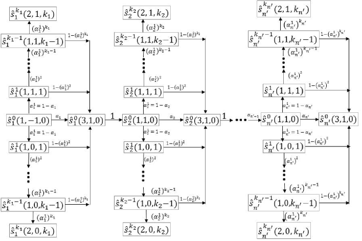
In order to determine the number of replicas for each primary active component as discussed in Section 4.2, we formulate the problem using discrete-time three-dimensional Markov Decision Process (MDP) model as depicted in Figure 2. MDP models are useful when the whole system is a discrete-time stochastic control process. It is also applied in addressing different research challenges of cloud computing such as resource management [32], QoS [33], resource and service failure management [34], etc. As we need to make the decision on the type and number of replicas for each component, which is dynamic in nature due to the respective failure probability, it is highly essential to model the problem with a tool that can take the fully observable states of this controlled systems into consideration.

Based on the failure probability of a component, the number of states is decided. A state represents either a primary or a backup component. A component with higher failure probability may have a larger number of states that may run either in parallel or sequential manner. The MDP can be represented as 3-tuple $\{\hat{S},U,\hat{\alpha}\}$, where $\hat{S}$ represents the state space, $U$ represents the action set that needs to be performed in every state, and $\hat{\alpha}$ represents the set of transition probabilities between two adjacent states.

Figure 2: Proposed Markov decision process model

5.1 State space

As discussed earlier, the state of a component represents the execution order of either a primary component or a backup component, which may run either in parallel or sequential order. In the proposed MDP model, the state of a component $\hat{c}_{i},1\leq i\leq n$ is represented as $\hat{s}_{i}^{j}(\ddot{c}_{i}^{j},\ddot{o}_{i}^{j},\ddot{b}_{i}^{j})$. $\hat{S}$ is the set of states for all primary and backup components. A state captures three essential information. Those are (a) the status of the component, (b) order of execution of corresponding components, and (c) number of backup components. Here, the value of superscript $j$ is dynamic and the maximum value of $j$ for each component may vary depending on the failure probability of the component. Value of $j=0$ represents that the state is for the primary component. However, value of $j\geq 1$ indicates that the state is for a backup component. For example, state $\hat{s}_{1}^{0}$ represents the primary component of component $\hat{c}_{1}$, whereas the state $\hat{s}_{1}^{2}$ represents the $2^{nd}$ backup component of the component $\hat{c}_{1}$. The status of an active component $\hat{c}_{i}$ could be running, rejected or finished, which is represented as $\ddot{c}_{i}^{j}$. Mathematically,

$$\ddot{c}_{i}^{j}=\left\{\begin{array}[]{ll}1&\text{If component }\hat{c}_{i}\text{ is in running state.};\\ 2&\text{If component }\hat{c}_{i}\text{ is rejected.};\\ 3&\text{If component }\hat{c}_{i}\text{ is finished its execution.};\end{array}\right.$$ (31)

The order of execution of a replica component is represented as $\ddot{o}_{i}^{j}$ of the active component $\hat{c}_{i}$. Mathematically, the value of $\ddot{o}_{i}^{j}$ can be written as follows.

$$\ddot{o}_{i}^{j}=\left\{\begin{array}[]{ll}0&\text{If the replica components are scheduled to run }\\ &\text{concurrently.}\\ 1&\text{If the replica components are scheduled to run }\\ &\text{sequentially.}\\ -1&\text{Otherwise.}\end{array}\right.$$ (32)

The order of execution $\ddot{o}_{i}^{j}$ for the order component is -1. For example, the value of $\ddot{o}_{i}^{j}$ of the components $c_{1},c3,$ and $c4$ in Figure 1 is $-1$. This indicates that such primary active components need to be scheduled at the very beginning and do not depend on any other components. The replica components can be scheduled to run concurrently, represented by 0, or sequentially, represented by 1, as shown in Figure  2. However, as discussed earlier, the execution order of replica components of the primary components must follow the Constraint 21. In other words, replicas of higher-ranked primary component must be scheduled to execute concurrently and the replicas of lower-ranked primary component must be scheduled to run sequentially.

Eventually, the number of replica components is considered as the third dimension of a state. The number of replicas of the component $\hat{c}_{i}$ is represented as $\ddot{b}_{i}^{j}$. For example, the state $\hat{s}_{2}^{2}(1,1,2)$ indicates that two replicas of the component $\hat{c}_{2}$ are scheduled to run sequentially.

5.2 Action space

The set of actions that is available at every state is represented as $U$. Any one of the three actions can be taken at each state, such as (a) Create new backup denoted as $u_{1}$, (b) Reject the component, denoted as $u_{2}$, and (c) Execute the component, denoted as $u_{3}$. Based on the failure probability of the components, actions are applied to the states. For example, applying the action $u_{3}$ with the success probability $\alpha_{1}$ onto the state $\hat{s}_{1}^{0}(1,-1,0)$, the resultant state would be $\hat{S}_{1}^{0}(3,1,0)$. Similarly, applying the action $u_{1}$ onto the state $\hat{S}_{1}^{0}(1,-1,0)$, the resultant state would be $\hat{S}_{1}^{1}(1,0,1)$.

5.3 State transition probability

It is assumed that $\alpha_{i}$ be the success probability of the primary active component $\hat{c}_{i},1\leq i\leq n$ with no corresponding replica components. Mathematically, the transition probability from the state $\hat{s}_{i}^{0}(1,\ddot{o}_{i}^{0},0)$ to $\hat{s}_{i}^{0}(3,1,0)$ with the action $u_{3}$ is $\alpha_{i}$.

$$Pr(\hat{s}_{i}^{0}(3,1,0)|\hat{s}_{i}^{0}(1,\ddot{o}_{i}^{0},0),u_{3})=\alpha_{i},\quad 1\leq i\leq n$$ (33)

From Equation 33, it can be derived that the failure probability of the component $\hat{c}_{i}$. In order to reduce the failure probability of a component, multiple replicas can be scheduled to run either in parallel or sequential order. Hence, the probability of creating the initial replica can be calculated as $1-\alpha_{i}$. Mathematically,

$$\alpha_{i}^{1}=Pr(\hat{s}_{i}^{1}(1,\ddot{o}_{i},1)|\hat{s}_{i}^{0}(1,\ddot{o}_{i}^{0},0),u_{1})=1-\alpha_{i},\quad 1\leq i\leq n$$ (34)

Here, $\alpha_{i}^{1}$ represents the transition probability from the state $\hat{s}_{i}^{0}$ to the state $\hat{s}_{i}^{1}$. In general, the notation $\alpha_{i}^{j}$ represents the transition probability from the state $\hat{s}_{i}^{j-1}$ to the state $\hat{s}_{i}^{j},1\leq j$. As discussed earlier in Section 4.2, $\bigtriangledown$ is defined as the minimum permissible failure probability. The number of replica components depend on the value of $\bigtriangledown$. The condition to apply the action $u_{1}$ onto any state can be written as follows.

$$Pr(\hat{s}_{i}^{j+1}(1,\ddot{o}_{i}^{j},\ddot{b}_{i}^{j+1})|\hat{s}_{i}^{j}(1,\ddot{o}_{i}^{j},\ddot{b}_{i}^{j}),u_{1})>\bigtriangledown$$ (35)

In other words, a new replica component (i.e. to state $\hat{s}_{i}^{j+1}(1,\ddot{o}_{i}^{j},\ddot{b}_{i}^{j+1})$) needs to be created (from the state $\hat{s}_{i}^{j}(1,\ddot{o}_{i}^{j},\ddot{b}_{i}^{j})$) of the component $\hat{c}_{i}$, by applying the action $u_{1}$, if the failure probability of the component is greater than $\bigtriangledown$.

From Equation 34 and 35, and with the given value of $\ddot{o}_{i}^{j}$, the order of execution of the replicas of the primary active component $\hat{c}_{i}$, the number of replica components can be determined from the following relation.

$$(1-\alpha_{i})^{k_{i}}\leq\bigtriangledown$$ (36)

Where, $k_{i}$ is the number of replica components of the primary active component $\hat{c}_{i}$. Further, using Equation 36, the value of $k_{i}$ can be derived as follows.

$$(1-\alpha_{i})^{k_{i}}\leq\bigtriangledown$$

$$\qquad\Longrightarrow k_{i}*log(1-\alpha_{i})\leq log(\bigtriangledown)$$

$$\qquad\Longrightarrow k_{i}=\lceil log_{(1-\alpha_{i})}(\bigtriangledown)\rceil$$ (37)

In the following subsection, we will present a numerical example to illustrate the workings of our proposed MDP.

5.4 Markov model example

Figure 3: An example of proposed MDP model

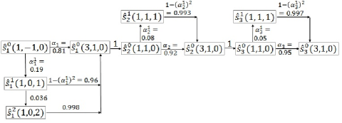
In order to illustrate the proposed MDP model presented in Figure 2, let us assume a cloud application with three components $\hat{c}_{1},\hat{c}_{2},$ and $\hat{c}_{3}$. Component $\hat{c}_{2}$ and $\hat{c}_{3}$ depends on $\hat{c}_{1}$ and $\hat{c}_{2}$, respectively. The initial state for component $\hat{c}_{1}$ can be written as $\hat{s}_{1}^{0}(\ddot{c}_{1}^{0}=1,\ddot{o}_{1}^{0}=-1,\ddot{b}_{1}^{0}=0)$. Similarly, for the component $\hat{c}_{2}$ and $\hat{c}_{3}$, the states can be written as $\hat{s}_{2}^{0}(1,1,0)$ and $\hat{s}_{3}^{0}(1,1,0)$, respectively. The value of $\ddot{o}_{2}^{0}$ and $\ddot{o}_{3}^{0}$ for component $\hat{c}_{2}$ and $\hat{c}_{3}$ is 1 as both components run sequentially after the component $\hat{c}_{1}$. Let, the failure probability of the component $\hat{c}_{1},\hat{c}_{2},$ and $\hat{c}_{3}$ be $0.19,0.08,$ and $0.05$, respectively, and the value of minimum permissible failure probability $\bigtriangledown$ be $0.007$.

For the above scenario, the MDP is presented in Figure 3. In Figure 3, the transition probability from the state $\hat{s}_{1}^{0}(1,-1,0)$ to state $\hat{s}_{1}^{1}(1,0,1)$ is $0.19$. State $\hat{s}_{1}^{1}(1,0,1)$ represents the first backup component of the primary component $\hat{c}_{1}$ and is scheduled to run in parallel. The failure probability of the first backup component is calculated to be $0.036$, which is still greater than the permissible failure probability $\bigtriangledown=0.007$. As a result, the second backup component is created and is represented as the state $\hat{s}_{1}^{2}(1,0,2)$. Since, the failure probability of the state $\hat{s}_{1}^{2}(1,0,2)$ is calculated to be $0.002$, which is less than $\bigtriangledown$, no further backup component is created. Similarly, the failure probability of the component $\hat{c}_{2}$ is $0.08$, which is greater than the value of $\bigtriangledown$. In order to reduce the failure probability, another backup component $\hat{s}_{2}^{1}(1,1,1)$ is created, which is scheduled to run in a sequential manner. The state $\hat{s}_{3}^{0}(3,1,0)$ represents that the component $\hat{c}_{3}$ has finished its execution.

5.5 Policy optimization

Using the proposed Three-dimensional MDP model as discussed above, we optimize the policy of determining the total number of replica components for all primary active components. Mathematically,

$$Minimize\text{ }K=\sum_{i=1}^{n}k_{i},\qquad 1\leq i\leq n$$ (38)

where, $K$ is the sum of number of replica components for all primary active components. In order to optimize the value of $K$, it is necessary to minimize the value of $k_{i}$ for each component. However, the policy must follow the constraint mentioned in Constraint 21. In other words, replicas of the component with the highest rank must be scheduled to run in parallel and the replicas of the component with lower rank must be scheduled to execute in sequential manner. This will support our belief that most significant components must finish their execution with higher degree of fault tolerant without violating the deadline. On the other hand, replicas of the lower rank components are allowed to take longer time in case of any failure as the failure of lower rank components has a trivial impact on other components.

6 Performance Evaluation

In order to evaluate the performance of the proposed RRFT strategy, the proposed component ranking and placement scheme is implemented on MATLAB platform. The cloud applications are generated randomly and are presented in matrix array. The cloud applications with varied numbers of components are generated using different probabilistic approaches such as arrival of cloud application from users that follows the Poisson distribution. We compare our component ranking method against two popular ranking algorithms, i.e., FTCloud [10] and ROCloud [23]. In FTCloud, component invocation structure and invocation frequencies parameters are used to rank the most significant components. Another version of the algorithm combines the application designer knowledge to find the critical and non-critical component and the system structure to rank the cloud components. On the other hand, the algorithm proposed in ROCloud uses failure rate and the failure impact as the reliability properties of the components. The extended version of ROCloud considers the hybrid applications, which consists of components that can be migrated to the public cloud and some components that can be scheduled to run in private cloud.

Further, the proposed component placement algorithm is evaluated and compared with random placement method. The cloud application is presented in DAG, which indicates that the adjacency matrix does not contain any circle. The failure rate of the components follows Poisson distribution in the simulation. The active time of the components is assumed to be known, which is assigned randomly in the simulation. In order to reduce the impact of a single failure of a physical machine, one PM is assigned to host one component from one cloud application. The number of components in each cloud application is randomly distributed, ranging from $4$ through $16$. In such scenarios, the minimum number of required PMs will range from $4$ through $20$. The probability that two components are connected could range from $0.5$ through $0.8$. The memory and CPU resource requirement of the components follows the random distribution ranging from $1000MB$ through $2000MB$ and from $1$ through $4$, respectively. Similarly, the memory and CPU capacity of the PMs are distributed randomly, ranging from $16000MB$ to $32000$ and $16$ to $32$, respectively. Taking above-mentioned performance matrix, following simulation results are obtained.

6.1 Simulation Results

Figure 4: Number of required VMs.

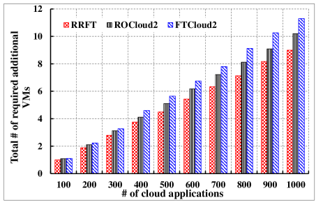
The performance of the proposed scheme is compared with ROCloud2 and FTCloud2 algorithm, as discussed before. The comparison results are shown in Figure 4 and 5. The results shown in Figure 4 reveal the total number of VMs required for a certain number of cloud applications. The number of cloud application varies from $100$ to $1000$. It is observed from the simulation result that the total number of VMs required for $100$ cloud applications is $996$, $1090$, and $1107$ for the proposed RRFT algorithm, ROCloud2, and FTCloud2 algorithms, respectively. However, the number increases to $9010,10205,$ and $11317$ for $1000$ numbers of cloud applications in case of RRFT, ROCloud2, and FTCloud2 algorithms, respectively. This shows approximately a 10% reduction in the required number of VMs when the number of cloud applications is 1000. It is expected that the RRFT algorithm would give similar result even after deploying more than 1000 cloud applications. In the simulation setup, the number of components per cloud application ranges from $4$ to $16$.

Figure 5: Number of required PMs.

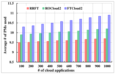
Similarly, the number of PMs used to host a certain number of cloud applications is shown in Figure 5. The value along Y-axis shows the average number of PMs used to host certain number of cloud applications. For example, the average number of PMs used to execute $100$ numbers of cloud applications is $9.5$ in the case of proposed RRFT algorithm. However, in case of ROCloud2 and FTCloud2 algorithm, the average number of PMs used is $9.9$ and $10.3$, respectively, which is at least 4.2% more than that of RRFT algorithm. The required number of PMs increases to $9.7,10.2,$ and $10.9$ for $1000$ number of cloud applications while executing the RRFT, ROCloud2, and FTCloud algorithm, respectively.

Figure 6: Number of VMs required under different order of execution of components.

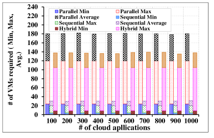
Under the proposed scheme, the components are scheduled to run under both parallel and sequential orders. The components that are more likely to fail are scheduled to run in a parallel manner along with their corresponding backup components. In other words, the higher-rank backup components are scheduled to run in parallel manner and rest of the components are scheduled to run in the sequential manner. The effects of order of executions of the backup components on amount of resource requirement and the recovery time are shown in Figure 6 and 7. Figure 6 shows the effect of the execution order of backup components onto the number of required VMs. In the simulation, $5$ backup components are scheduled for each component in case of parallel and sequential order of execution. It is found that for $100$ cloud applications, each consisting of $4$ to $16$ number of components, a minimum of $24$, maximum of $96$, and an average of $51.11$ numbers of VMs required per application, when the backup components are scheduled to run in concurrent manner. However, the number of VMs falls to an average of $10.22$ numbers of VMs, when all the backup components are scheduled to run in sequential manner. The minimum and maximum numbers of VMs required in sequential manner are $4$ and $16$, respectively, which is equal to the minimum and maximum number of components present in a cloud application. In hybrid mode, the additional requirement of resources in terms of number of VMs is higher than that of the sequential order but lesser than that of the parallel order as backup components are scheduled to run in both parallel and sequential mode. The minimum, maximum, and the average number of VMs required for $100$ numbers of cloud applications are $9,96,$ and $32.57$. In the simulation setup, the backup components of at least one component are scheduled to run in concurrent manner, and hence a minimum of $9$ numbers of VMs is required for the proposed hybrid order of VM execution.

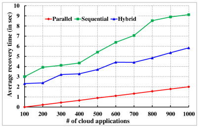
The order of execution also has an impact on recovery time. The recovery time is defined as the time required to recover the service from the corresponding component failure. In case of the parallel execution of the backup components, the recovery time is very less, which ranges from $0$ to $2$ seconds for the number of components ranging from $100$ to $1000$, as shown in Figure 7. However, in case of sequential execution of backup components, the recovery time is very high as one component needs to restart from the very beginning of its failure. The recovery time for sequential execution of the backup components ranges from $3sec$ to $9.12sec$ for $100$ components to $1000$ components. According to the proposed algorithm, the order of execution of backup components is hybrid. Hence, it is observed that the recovery time for same number of components ranges from approximately $2.3sec$ to $5.84sec$.

Figure 7: Recovery time under different order of execution of components.

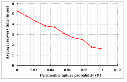
The impacts of permissible failure probability $(\bigtriangledown)$ on the additional resource requirement and recovery time are investigated and the results are presented in Figure 8 and 9. The backup components are created based on the value of $(\bigtriangledown)$. Backup components are not created for components with the failure probability less than $(\bigtriangledown)$. Hence, the component with higher value of $(\bigtriangledown)$ requires more number of backup components. This is also reflected in the simulation result presented in Figure 8.

Figure 8: The impact of permissible failure probability on resource requirement.

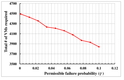
The amount of required resources decreases when the value of $(\bigtriangledown)$ increases as discussed in Figure 8. Hence, it is obvious that the recovery time would decrease with the increase in permissible failure probability $(\bigtriangledown)$. The value of $(\bigtriangledown)$ ranges from $0.001$ to $0.1$. It is observed that the recovery time also decreases from approximately $5.25sec$ to $1.6sec$, when the value of $(\bigtriangledown)$ increases. The results in Figure 8 and 9 are obtained by keeping the number of cloud components to $500$.

Figure 9: The impact of permissible failure probability on recovery time.

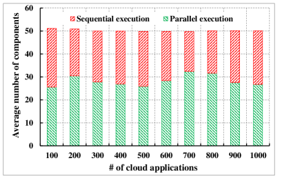
In the proposed Hybrid k* fault tolerant strategy, the backup components are scheduled to run in both parallel and sequential order. Further, the number of backup components also varies based on the value of $\bigtriangledown$. In Figure 10, average number of components along Y-axis refers to as the sum of number of primary and backup components. For $100$ number of cloud applications, the average number of backup components scheduled to run in parallel and sequential order is $25.59$ and $25.51$, respectively. However, when the number of cloud application increases to $1000$, the average number of backup components running in parallel and sequential order is $26.76$ and $23.30$, respectively. It is observed that the number of backup components running in parallel and sequential order are almost similar. Here, the number of primary components for each cloud application ranges from $4$ to $15$, with an average of $10$.

Figure 10: Number of parallel and sequential backup components.

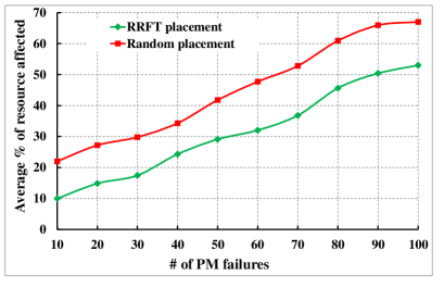
Considering the placement strategy as one of the performance metrics, the effect of random placement and the proposed component placement scheme onto the impact of PM failures are compared and presented in Figure 11. A single PM failure may bring down multiple primary and backup components. The number of PM failures ranges from $10$ to $100$. The average percentage of resource affected is calculated by obtaining the ratio of number of VMs failed and the total number of VM currently allocated to each cloud application. During the simulation, the number of cloud applications is set to be $1000$. When the components are placed onto random physical machines, it is observed that the percentage of the resource affected is very high as compared to that of the proposed component placement scheme. The percentage of resource affected ranges from $22\%$ to $67\%$, when the components are placed randomly. However, the percentage of resource failure ranges between $10\%$ to $53\%$ when the components are placed by following the proposed component placement scheme, which is at least 20% lesser over the random placement of the component.

Figure 11: The impact of PM failures onto the allocated virtual resources.

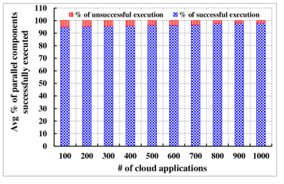
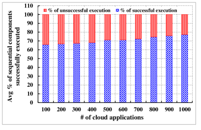
As a subset of the backup components is scheduled to run in parallel order, it is essential to examine if those backup components are executed successfully. The percentage of backup components that are running concurrently and have finished their execution successfully is presented in Figure 12. In other words, the values in Y-axis represents the percentage of concurrently scheduled backup components that are executed successfully and unsuccessfully. It is observed from the simulation results that the percentage of backup components executed successfully ranges between $95\%$ to $98\%$, when the number of cloud components ranges between $100$ and $1000$. Hence, the percentage of components that are unable to finish the execution ranges from $5\%$ to $2\%$.

Figure 12: Percentage of parallel backup components successfully executed.

Similarly, the percentage of backup components that are scheduled to run in sequential order and are executed successfully is examined and presented in Figure 13. It is observed that approximately $66\%$ of the backup components are successfully executed when the number of cloud components is $100$. The percentage increases to approximately $78\%$, when the number of cloud components increases to $1000$. We can conclude here that with an increase in the number of cloud components, the percentage of failure execution of sequentially scheduled backup components decreases. However, the percentage value along Y-axis will remain saturated when the number of cloud application increases further.

Figure 13: Percentage of sequential backup components successfully executed.

7 Conclusions and Future works

In this paper, we addressed an important problem of providing fault tolerant services to the cloud components based on their ranking. As providing fault tolerant services could be resource-intensive, our objective was to minimize the amount of additional resources required to provide the fault tolerant services. It is assumed that the cloud applications comprise multiple cloud components. The significance or importance level of all cloud components with respect to a particular cloud application is different. Hence, we first proposed a mechanism to find out the most significant component, based on which ranking of the component is done. Following the ranking mechanism, Hybrid k* fault tolerant strategy is proposed with the objective to provide the maximum degree of fault tolerant to the components with higher rank values and to provide minimum amount of additional resources to the components with lower rank values. Besides, a component placement strategy is proposed with the objective to find a suitable PM for each primary and backup component. The objective of proposing the component placement strategy is also to reduce the impact of single PM failure onto single cloud application.

The proposed scheme is evaluated with the similar component ranking and fault tolerance strategies. It is observed that the proposed RRFT algorithm reduced the required number of VMs and PMs by approximately 10% and 4.2%, respectively. With the proposed placement strategy, the percentage of virtual resource affected due to failure of a PM is found to be at least 20% lesser than that of random placement strategy. However, extending the current version of the algorithm by considering other parameters such as makespan, user priority, cost of each components etc. and experimenting the extended version of the proposed algorithm in real environment would be the part of our future works as it is hard to build a simulated environment with exact configuration of real environment. In addition to this, we will also divert our focus to investigate the difference in characteristics of VMs and containers and make the proposed algorithm more applicable to the micro-service and container-based cloud application.

Chinmaya Kumar Dehury Chinmaya Kumar Dehury received bachelor degree from Sambalpur University, India, in June 2009 and MCA degree from Biju Pattnaik University of Technology, India, in June 2013. He received the PhD Degree in the department of Computer Science and Information Engineering, Chang Gung University, Taiwan. He is currently a Lecturer of Distributed System, member of Mobile & Cloud Lab in the Institute of Computer Science, University of Tartu, Estonia. His research interests include scheduling, resource management and fault tolerance problems of Cloud and fog Computing, and the application of artificial intelligence in cloud management. He is a member, IEEE, and also reviewer to several journals and conferences, such as IEEE TPDS, IEEE JSAC, Wiley Software: Practice and Experience, etc.

Prasan Kumar Sahoo Prasan Kumar Sahoo received the B.Sc. degree in physics (with Honors), the M.Sc. degree in mathematics both from Utkal University, Bhubaneswar, India, in 1987 and 1994, respectively. He received the M.Tech. degree in computer science from the Indian Institute of Technology (IIT), Kharagpur, India, in 2000, the first Ph.D. degree in mathematics from Utkal University, in 2002, and the second Ph.D. degree in computer science and information engineering from the National Central University, Taiwan, in 2009. He is currently a Professor in the Department of Computer Science and Information Engineering, Chang Gung University, Taiwan. He was an Adjunct Associate Researcher in the Department of Cardiology and was an Adjunct Researcher in the Division of Colon and Rectum Cancer, Chang Gung Memorial Hospital, Linkou, Taiwan. Currently, he is an Adjunct Researcher in the Department of Neurology, Chang Gung Memorial Hospital, Linkou, Taiwan . He has worked as an Associate Professor in the Department of Information Management, Vanung University, Taiwan, from 2007 to 2011. He was a Visiting Associate Professor in the Department of Computer Science, Universite Claude Bernard Lyon 1, Villeurbanne, France. His current research interests include artificial intelligence, big data analytic, cloud computing, and IoT. He is an Editorial Board Member of Journal of Network and Computer Applications, International Journal of Vehicle Information and Communication Systems and was Lead Guest Editor, special issue of Electronics journal. He has worked as the Program Committee Member of several IEEE and ACM conferences and is a senior member, IEEE.

Bharadwaj Veeravalli Bharadwaj Veeravalli received his BSc degree in Physics, from Madurai-Kamaraj University, India, in 1987, the Master’s degree in Electrical Communication Engineering from the Indian Institute of Science, Bangalore, India in 1991, and the PhD degree from the Department of Aerospace Engineering, Indian Institute of Science, Bangalore, India, in 1994. He received gold medals for his bachelor degree overall performance and for an outstanding PhD thesis (IISc, Bangalore India) in the years 1987 and 1994, respectively. He is currently with the Department of Electrical and Computer Engineering, Communications and Information Engineering (CIE) division, at The National University of Singapore, Singapore, as a tenured Associate Professor. His main stream research interests include cloud/grid/cluster computing (big data processing, analytics and resource allocation), scheduling in parallel and distributed systems, Cybersecurity, and multimedia computing. He is one of the earliest researchers in the field of Divisible Load Theory (DLT). He is currently serving the editorial board of IEEE Transactions on Parallel and Distributed Systems as an associate editor. He is a senior member of the IEEE and the IEEE-CS.

References

- [1] S. Ghazouani and Y. Slimani, “A survey on cloud service description,” Journal of Network and Computer Applications, vol. 91, pp. 61 – 74, 2017.
- [2] C. K. Dehury and P. K. Sahoo, “DYVINE: Fitness-Based Dynamic Virtual Network Embedding in Cloud Computing,” IEEE Journal on Selected Areas in Communications, vol. 37, no. 5, pp. 1029–1045, May 2019.
- [3] Y. Ding, G. Yao, and K. Hao, “Fault-tolerant elastic scheduling algorithm for workflow in cloud systems,” Information Sciences, vol. 393, pp. 47 – 65, 2017.
- [4] I. Gog, M. Schwarzkopf, A. Gleave, R. N. M. Watson, and S. Hand, “Firmament: Fast, centralized cluster scheduling at scale,” in Proceedings of the 12th USENIX Conference on Operating Systems Design and Implementation, ser. OSDI’16. USA: USENIX Association, 2016, p. 99–115.
- [5] G. Yao, Y. Ding, and K. Hao, “Using imbalance characteristic for fault-tolerant workflow scheduling in cloud systems,” IEEE Transactions on Parallel and Distributed Systems, vol. PP, no. 99, pp. 1–1, 2017.
- [6] M. N. Cheraghlou, A. Khadem-Zadeh, and M. Haghparast, “A survey of fault tolerance architecture in cloud computing,” Journal of Network and Computer Applications, vol. 61, pp. 81–92, 2016.
- [7] P. He, X. Zhao, C. Tan, Z. Zheng, and Y. Yuan, “Evaluation and optimization of the mixed redundancy strategy in cloud-based systems,” China Communications, vol. 13, no. 9, pp. 237–248, Sept 2016.
- [8] M. Amoon, “Adaptive framework for reliable cloud computing environment,” IEEE Access, vol. 4, pp. 9469–9478, 2016.
- [9] W. Chen, R. F. da Silva, E. Deelman, and T. Fahringer, “Dynamic and fault-tolerant clustering for scientific workflows,” IEEE Transactions on Cloud Computing, vol. 4, no. 1, pp. 49–62, Jan 2016.
- [10] Z. Zheng, T. C. Zhou, M. R. Lyu, and I. King, “Component ranking for fault-tolerant cloud applications,” IEEE Transactions on Services Computing, vol. 5, no. 4, pp. 540–550, 2012.
- [11] P. Kumari and P. Kaur, “A survey of fault tolerance in cloud computing,” Journal of King Saud University - Computer and Information Sciences, 2018.
- [12] M. Hasan and M. S. Goraya, “Fault tolerance in cloud computing environment: A systematic survey,” Computers in Industry, vol. 99, pp. 156–172, 2018.
- [13] P. K. Sahoo, C. K. Dehury, and B. Veeravalli, “Lvrm: On the design of efficient link based virtual resource management algorithm for cloud platforms,” IEEE Transactions on Parallel and Distributed Systems, vol. 29, no. 4, pp. 887–900, April 2018.
- [14] G. Fan, L. Chen, H. Yu, and D. Liu, “Modeling and analyzing dynamic fault-tolerant strategy for deadline constrained task scheduling in cloud computing,” IEEE Transactions on Systems, Man, and Cybernetics: Systems, vol. 50, no. 4, pp. 1260–1274, April 2020.
- [15] H. Han, W. Bao, X. Zhu, X. Feng, and W. Zhou, “Fault-tolerant scheduling for hybrid real-time tasks based on cpb model in cloud,” IEEE Access, vol. 6, pp. 18 616–18 629, 2018.
- [16] A. R. Setlur, S. J. Nirmala, H. S. Singh, and S. Khoriya, “An efficient fault tolerant workflow scheduling approach using replication heuristics and checkpointing in the cloud,” Journal of Parallel and Distributed Computing, vol. 136, pp. 14 – 28, 2020.
- [17] G. Yao, Y. Ding, and K. Hao, “Using imbalance characteristic for fault-tolerant workflow scheduling in cloud systems,” IEEE Transactions on Parallel and Distributed Systems, vol. 28, no. 12, pp. 3671–3683, 2017.
- [18] Z. Wang, L. Gao, Y. Gu, Y. Bao, and G. Yu, “A fault-tolerant framework for asynchronous iterative computations in cloud environments,” IEEE Transactions on Parallel and Distributed Systems, vol. 29, no. 8, pp. 1678–1692, Aug 2018.
- [19] D. J. Dean, H. Nguyen, P. Wang, X. Gu, A. Sailer, and A. Kochut, “Perfcompass: Online performance anomaly fault localization and inference in infrastructure-as-a-service clouds,” IEEE Transactions on Parallel and Distributed Systems, vol. 27, no. 6, pp. 1742–1755, 2016.
- [20] B. Ray, A. Saha, S. Khatua, and S. Roy, “Proactive fault-tolerance technique to enhance reliability of cloud service in cloud federation environment,” IEEE Transactions on Cloud Computing, pp. 1–1, 2020.
- [21] G. Yuan, Z. Xu, B. Yang, W. Liang, W. K. Chai, D. Tuncer, A. Galis, G. Pavlou, and G. Wu, “Fault tolerant placement of stateful vnfs and dynamic fault recovery in cloud networks,” Computer Networks, vol. 166, p. 106953, 2020.
- [22] S. Deng, L. Huang, J. Taheri, and A. Y. Zomaya, “Computation offloading for service workflow in mobile cloud computing,” IEEE Transactions on Parallel and Distributed Systems, vol. 26, no. 12, pp. 3317–3329, 2015.
- [23] W. Qiu, Z. Zheng, X. Wang, X. Yang, and M. R. Lyu, “Reliability-based design optimization for cloud migration,” IEEE Transactions on Services Computing, vol. 7, no. 2, pp. 223–236, 2014.
- [24] Y. Wang, Q. He, D. Ye, and Y. Yang, “Formulating criticality-based cost-effective fault tolerance strategies for multi-tenant service-based systems,” IEEE Transactions on Software Engineering, vol. 44, no. 3, pp. 291–307, March 2018.
- [25] M. Smara, M. Aliouat, A.-S. K. Pathan, and Z. Aliouat, “Acceptance test for fault detection in component-based cloud computing and systems,” Future Generation Computer Systems, 2016.
- [26] T. Wang, W. Zhang, C. Ye, J. Wei, H. Zhong, and T. Huang, “Fd4c: Automatic fault diagnosis framework for web applications in cloud computing,” IEEE Transactions on Systems, Man, and Cybernetics: Systems, vol. 46, no. 1, pp. 61–75, 2016.
- [27] C.-A. Chen, M. Won, R. Stoleru, and G. G. Xie, “Energy-efficient fault-tolerant data storage and processing in mobile cloud,” IEEE Transactions on cloud computing, vol. 3, no. 1, pp. 28–41, 2015.
- [28] P. Gupta and S. Ghrera, “Power and fault aware reliable resource allocation for cloud infrastructure,” Procedia Computer Science, vol. 78, pp. 457–463, 2016.
- [29] J. Wang, W. Bao, X. Zhu, L. T. Yang, and Y. Xiang, “Festal: fault-tolerant elastic scheduling algorithm for real-time tasks in virtualized clouds,” IEEE Transactions on Computers, vol. 64, no. 9, pp. 2545–2558, 2015.
- [30] K. Vinay and S. M. D. Kumar, “Fault-tolerant scheduling for scientific workflows in cloud environments,” in 2017 IEEE 7th International Advance Computing Conference (IACC), Jan 2017, pp. 150–155.
- [31] R. T. Anderson, “Reliability design handbook,” RELIABILITY ANALYSIS CENTER GRIFFISS AFB NY, Tech. Rep., 1976.
- [32] M. Shifrin, R. Mitrany, E. Biton, and O. Gurewitz, “Vm scaling and load balancing via cost optimal mdp solution,” IEEE Transactions on Cloud Computing, pp. 1–1, 2020.
- [33] H. Liang, X. Wen, Y. Liu, H. Zhang, L. Zhang, and L. Wang, “Logistics-involved qos-aware service composition in cloud manufacturing with deep reinforcement learning,” Robotics and Computer-Integrated Manufacturing, vol. 67, p. 101991, 2021.
- [34] C. Li, Y. Wang, Y. Chen, and Y. Luo, “Energy-efficient fault-tolerant replica management policy with deadline and budget constraints in edge-cloud environment,” Journal of Network and Computer Applications, vol. 143, pp. 152–166, 2019.
![[Uncaptioned image]](/html/2111.00579/assets/x14.png) |