Density of Bloch states inside a one dimensional photonic crystal

Abstract

The density of Bloch electromagnetic states inside a one dimensional photonic crystal (1D PC) is formulated based on its dispersion relations. The formulation applied to any anisotropic medium with known dispersion relations and iso-frequency surfaces. Using a practical 1D PC parameters in the visible range, the density of Bloch states for different modes are calculated.

Introduction

The density of electromagnetic modes/states (DOS) is an important quantity in statistical physics. It is often used as the degeneracy function for the energy levels in thermal radiation studies such as Planck’s blackbody radiation [1, 2]. Consider the distribution of photons inside a large cavity in thermal equilibrium with a solid matter at temperature T (a.k.a. cloud of photons). The solid matter provides the mechanism to convert photons energies (i.e. annihilate and create them) according to the temperature. Since photons are bosons, the number of photons at each energy level ($\varepsilon_{i}=\hbar\omega$) follows Bose-Einstein distribution as [3]

$$n_{i}=\frac{g_{i}}{e^{-\alpha-\beta\varepsilon_{i}}-1}$$ (1)

where $g_{i}$ and $n_{i}$ are the degeneracy and photon number of each energy level ($\varepsilon_{i}$), respectively. Equation (1) is obtained by maximizing the number of micro-states in the system (see [3]). The constants $\alpha$ and $\beta$ are determined by enforcing the conditions $\sum n_{i}=N,$ and $\sum\varepsilon_{i}n_{i}=U$ where $N$ and $U$ are the total number and energy of bosons, respectively. The later condition leads to $\beta=\frac{1}{k_{B}T}$ where $k_{B}$ is Boltzmann’s constant, and the former does not apply to photons, as they can be created and annihilated bythe solid matter. This leads to setting $\alpha=0$. The modes degeneracy, $g_{i},$ is where the DOS is required. If there is no photons reflection at the surface of the thermal radiator (i.e. an ideal black body,) the DOS inside the thermal radiator is essentially the same as its ambient medium.

Alternatively, we could explain thermal emission by considering the distribution of emitters inside a matter at temperature T, and relate it to the radiational modes. An example of such methods is briefly reviewed in the appendix, for self-consistency.

If the emitting body is a 1D PC, the DOS consists of two contributions: Bloch states which can propagate and depart a finite-size 1D PC, and the wave-guided states which trap photons inside the 1D PC (mostly within higher permittivity layers). A complete analysis of these states is performed in [4] based on Green’s tensor approach. However, the density of Bloch states ($\mathrm{DOS_{Bloch}}$) can be calculated, exactly, using their dispersion relations in the 1D PC. This is the parameter which, depending on the geometry, can be used directly or indirectly as the degeneracy function in thermal emission from 1D PCs.

$\mathrm{DOS}_{\mathrm{Bloch}}\left(\omega\right)$ inside a 1D PC

We start by formulating the DOS inside a medium with known dispersion relations, and general non-spherical iso-frequency surfaces. The conventional method of calculating the DOS is to consider a large rectangular cavity with size L in all dimensions, filled with the medium, and with periodic boundary conditions on its walls. Eigen solutions of the harmonic electromagnetic wave equation, at frequency $\omega,$ in such geometry are modes in the form

$$F_{mnl}=C_{mnl}^{p}e^{-i\omega t}e^{i\left(\frac{2\pi m}{L}x+\frac{2\pi n}{L}y+\frac{2\pi l}{L}z\right)}$$ (2)

where $F_{mnl}$ is an electric (magnetic) field component of the mode and $C_{mnl}^{p}$ is its associated coefficient (which has both frequency and geometry dependences.) The superscript $p$ in $C_{mnl}^{p}$ denotes the mode’s polarization and can take two values (any two orthogonal polarizations is correct, but transverse electric and transverse magnetic modes along a cartesian coordinate axis are commonly chosen.) The values in the triplet $\left(m,n,l\right)$ can be any positive integer number subject to an equation obtained from the eigen value problem

$$f\left(\frac{2\pi m}{L},\frac{2\pi n}{L},\frac{2\pi l}{L},\omega\right)=0,$$ (3)

Equation (3) is known as the dispersion equation after defining and replacing the wave-vectors as

$$\left(k_{x},k_{y},k_{z}\right)=\left(\frac{2\pi m}{L},\frac{2\pi n}{L},\frac{2\pi l}{L}\right).$$ (4)

In case of an isotropic homogenous material, equation (3) becomes $\left(\frac{2\pi m}{L}\right)^{2}+\left(\frac{2\pi n}{L}\right)^{2}+\left(\frac{2\pi l}{L}\right)^{2}=k_{0}^{2}\varepsilon_{r}\mu_{r}$. The density of electromagnetic modes, $\mathrm{DOS}\left(\omega\right),$ is defined as the spectral density of the modes per cavity volume. That is, $\mathrm{DOS}\left(\omega\right)d\omega$ is the number of supported modes per volume in the interval $\left[\omega,\omega+d\omega\right]$,

$$\mathrm{DOS}\left(\omega\right)d\omega=\underset{\left\{\left(m,n,l\right):f\left(\frac{2\pi m}{L},\frac{2\pi n}{L},\frac{2\pi l}{L},\omega<\omega^{\prime}\leq\omega+d\omega\right)=0\right\}}{\sum\frac{2}{L^{3}}}$$ (5)

where the factor of 2 accounts for the two possible orthogonal polarizations per mode. We used the notation $\left\{x:p\left(x\right)\right\}$ which refers to the set of $x$ for which $p\left(x\right)$ is true. We may write (5) as

$$\mathrm{DOS}\left(\omega\right)d\omega=\underset{\left\{\left(m,n,l\right):f\left(\frac{2\pi m}{L},\frac{2\pi n}{L},\frac{2\pi l}{L},\omega<\omega^{\prime}\leq\omega+d\omega\right)=0\right\}}{\sum\frac{2}{L^{3}}\triangle m\triangle n\triangle l}$$ (6)

since $m,n,$ and $l$ are all integers, that is $\triangle m=\triangle n=\triangle l=1.$ Replacing (4) in (6) and converting the summation to the integration (since L is large) gives

$$\mathrm{DOS}\left(\omega\right)d\omega=\frac{2}{\left(2\pi\right)^{3}}\underset{\left\{\left(k_{x},k_{y},k_{z}\right):f\left(k_{x},k_{y},k_{z},,\omega<\omega^{\prime}\leq\omega+d\omega\right)=0\right\}}{\iiintop dV_{k}}$$ (7)

where $dV_{k}=dk_{x}dk_{y}dk_{z}$ is the volume differential in k- space. The integration in (7) is a volume (three-fold) integration between the two 3D surfaces in k- space, satisfying dispersion equation (3) at $\omega$ and $\omega+d\omega$, respectively. These surfaces are also known as the iso-frequency surfaces. Solution of equation (7) gives the DOS. Equation (7) holds regardless of the shape of the iso-frequency surfaces, and can be used directly for simple surfaces. For example, since the iso-frequency surfaces of a homogeneous isotropic space are spherical, using $k_{x}^{2}+k_{y}^{2}+k_{z}^{2}=k^{2}$ in (7) gives

$$\mathrm{DOS}\left(\omega\right)d\omega=\frac{2}{\left(2\pi\right)^{3}}\intop_{\frac{\omega}{c}\sqrt{\varepsilon_{r}\mu_{r}}}^{\frac{\left(\omega+d\omega\right)}{c}\sqrt{\varepsilon_{r}\mu_{r}}}\intop_{0}^{\pi}\intop_{0}^{2\pi}k^{2}sin\theta d\varphi d\theta dk$$ (8)

which after simple manipulation leads to the known equation $\mathrm{DOS}\left(\omega\right)=\frac{\omega^{2}\left(\mu_{r}\varepsilon_{r}\right)^{3/2}}{\pi^{2}c^{3}}.$

We may prepare (7) further for an arbitrary iso-frequency surface in k-space. This preparation becomes useful in finding $\mathrm{DOS_{Bloch}}\left(\omega\right)$ in photonic crystals and other non-trivial and anisotropic materials such as hyperbolic metamaterials where iso-frequency surfaces’ shapes depend on the frequency. For example, Fig. 1 shows the iso-frequency surfaces of a 1D PC at two nearby frequencies.

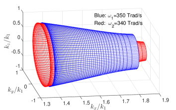
Figure 1: The iso-frequency surfaces of a 1D PC (TE modes) at two different frequencies normalized to $k_{1}=\omega\sqrt{\mu_{0}\varepsilon_{0}\varepsilon_{1}}.$ Parameters of the 1D PC are $T_{1}=300\>nm,$ $T_{2}=700\>nm,$ $\varepsilon_{1}=2.1,$ $\varepsilon_{2}=11.9.$

Each of the iso-frequency surfaces in (7) (and in Fig. 1) can be parametrized using two independent parameters $\theta$ and $\varphi$ as

$$S\left(\omega\right):\>\left(k_{x}\left(\theta,\varphi\right),k_{y}\left(\theta,\varphi\right),k_{z}\left(\theta,\varphi\right)\right)$$ (9)

where $\left(k_{x},k_{y},k_{z}\right)$ represents a vector in k-space. In general, the choice of parameters $\theta$ and $\varphi$ is arbitrary and depends on the shape of the iso-frequency surface. However, it is convenient to choose $\theta$ and $\varphi$ as spherical coordinate’s polar and azimuthal angles for 1D PCs. The surface differential for such arbitrary surface is

$$dA=\left\|t_{\theta}\times t_{\varphi}\right\|d\theta d\varphi$$ (10)

where $t_{\theta}$, $t_{\varphi}$ are tangential vectors to the surface as

$$t_{\theta}=\left(\frac{\partial k_{x}\left(\theta,\varphi\right)}{\partial\theta},\frac{\partial k_{y}\left(\theta,\varphi\right)}{\partial\theta},\frac{\partial k_{z}\left(\theta,\varphi\right)}{\partial\theta}\right),$$ (11)

$$t_{\varphi}=\left(\frac{\partial k_{x}\left(\theta,\varphi\right)}{\partial\varphi},\frac{\partial k_{y}\left(\theta,\varphi\right)}{\partial\varphi},\frac{\partial k_{z}\left(\theta,\varphi\right)}{\partial\varphi}\right),$$ (12)

and $\left\|.\right\|$ and $\times$ are the vector $L^{2}$ norm the external vector product, respectively. Since $t_{\theta}\times t_{\varphi}$ is a vector normal to the surface, the volume differential between the two iso-frequency surfaces at $\omega$ and $\omega+d\omega$ is

$$dV=\left|\left(S\left(\omega+d\omega\right)-S\left(\omega\right)\right).\left(t_{\theta}\times t_{\varphi}\right)d\theta d\varphi\right|,$$ (13)

which simplifies to

$$dV=\left|\left(\frac{\partial k_{x}}{\partial\omega},\frac{\partial k_{y}}{\partial\omega},\frac{\partial k_{z}}{\partial\omega}\right).\left(t_{\theta}\times t_{\varphi}\right)d\theta d\varphi d\omega\right|.$$ (14)

Note the $\left|.\right|$ operator is necessary in the volume calculations (since the volume between the two surfaces is independent of their order). Replacing (14) into (7) gives

$$\mathrm{DOS}\left(\omega\right)=\frac{2}{\left(2\pi\right)^{3}}\varoiintop_{S}\left|\left(\frac{\partial k_{x}}{\partial\omega},\frac{\partial k_{y}}{\partial\omega},\frac{\partial k_{z}}{\partial\omega}\right).\left(t_{\theta}\times t_{\varphi}\right)\right|d\theta d\varphi$$ (15)

which can be used for any iso-frequency surface provided that it can be parametrized. As a simple example, the spherical iso-frequency surfaces of a non-magnetic ($\mu_{r}=1$) homogeneous isotropic medium can be parametrized as

$$S:\>\left(\frac{\omega\sqrt{\varepsilon_{r}}}{c}sin\theta cos\varphi,\frac{\omega\sqrt{\varepsilon_{r}}}{c}sin\theta sin\varphi,\frac{\omega\sqrt{\varepsilon_{r}}}{c}cos\theta\right)$$ (16)

which easily leads to the expected result $\mathrm{DOS}\left(\omega\right)=\frac{\omega^{2}\varepsilon_{r}^{3/2}}{\pi^{2}c^{3}}.$

In a non-magnetic 1D PC, the dispersion relation is [5, 6]

$$k_{x}=\frac{1}{T_{1}+T_{2}}cos^{-1}\left(cos\left(k_{x1}T_{1}\right)cos\left(k_{x2}T_{2}\right)-\quad\right.$$ (17)

$$\qquad\qquad\left.0.5\left(\frac{p_{2}}{p_{1}}+\frac{p_{1}}{p_{2}}\right)sin\left(k_{x2}d_{2}\right)sin\left(k_{x1}d_{1}\right)\right),$$

where

$$k_{xi}=\sqrt{k_{i}^{2}-k_{y}^{2}-k_{z}^{2}};\;\quad p_{i}=\begin{cases}\begin{array}[]{c}\frac{k_{xi}}{\omega\mu_{0}}\\ \frac{\omega\varepsilon_{0}\varepsilon_{i}}{k_{xi}}\end{array}&\begin{array}[]{c}TE\\ TM\end{array}\end{cases},$$ (18)

and transverse electric (TE) and magnetic (TM) modes are defined with respect to the y-z plane (interface plane).

The iso-frequency surface of the 1D PC can be parametrized as

$$S\left(\theta,\varphi\right):\>k_{x}\left(\omega,\theta\right),\frac{\omega}{c}\sqrt{\varepsilon_{1}}cos\theta sin\varphi,\frac{\omega}{c}\sqrt{\varepsilon_{1}}cos\theta cos\varphi$$ (19)

where $(\theta,\varphi)$ are defined inside the material with the lower permittivity ($\varepsilon_{1}$) because the tangential wave-vector, $\sqrt{k_{y}^{2}+k_{z}^{2}}$, inside the PC cannot exceed $\frac{\omega}{c}\sqrt{\varepsilon_{min}}.$ The tangential vectors to the iso-frequency surface are

$$t_{\theta}:\>\left(\frac{dk_{x}\left(\omega,\theta\right)}{d\theta},-\frac{\omega}{c}\sqrt{\varepsilon_{1}}sin\theta sin\varphi,-\frac{\omega}{c}\sqrt{\varepsilon_{1}}sin\theta cos\varphi\right),$$ (20)

$$t_{\varphi}:\>\left(0,\frac{\omega}{c}\sqrt{\varepsilon_{1}}cos\theta cos\varphi,-\frac{\omega}{c}\sqrt{\varepsilon_{1}}cos\theta sin\varphi\right).$$ (21)

Using (15), (20), and (21), it is straight forward to show the density of Bloch states for TE and TM modes are

$$\mathrm{DOS}_{\mathrm{Bloch}}^{i}\left(\omega\right)=\frac{\omega\varepsilon_{1}}{4c^{2}\pi^{2}}\intop_{0}^{\pi}\left|\left(cos\theta\frac{\partial k_{x}^{i}\left(\omega,\theta\right)}{\partial\theta}+\omega sin\theta\frac{\partial k_{x}^{i}\left(\omega,\theta\right)}{\partial\omega}\right)cos\theta\right|d\theta,$$ (22)

where $i=\mathrm{TE}\>\mathrm{or}\>\mathrm{TM}$. Equation (22) can be solved, as is, using commercially available solvers and no further analytical expansion is necessary. However, special care should be given to the calculation of $k_{x}$ using (17) as it passes through different Riemann sheets, as will be further discussed later.

As an example, Fig. 2 shows the density of Bloch states inside a 1D PC with parameters $\varepsilon_{1}=11.9$, $\varepsilon_{2}=2.1$, $T_{1}=300\,\mathrm{nm}$, and $T_{2}=700\,\mathrm{nm}$. It also includes $\mathrm{DOS}$ of an isotropic homogeneous material with $\varepsilon_{1}=2.1$. Note that Bloch wave’s tangential wave-vector inside a 1D PC is always limited by the material with the lower permittivity (i.e. $\varepsilon_{1}$). The $\mathrm{DOS_{Bloch}}$ in Fig. 2 shows some dirivative discontinuities which are at frequencies near the band edges of TM or TE modes. Some of these local peaks exceed the DOS of an unbounded $\varepsilon_{1}$ region.

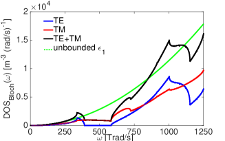
Figure 2: The Bloch density of states in the 1D PC. The DOS of an isotropic homogenous $\varepsilon_{1}=2.1$ medium is also shown as a reference.

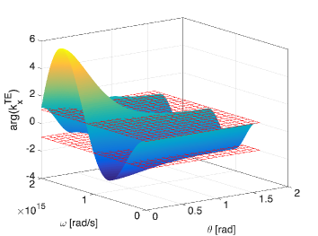
(a)

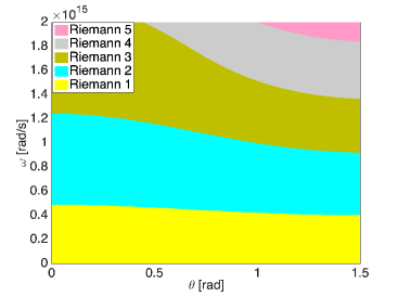
(b)

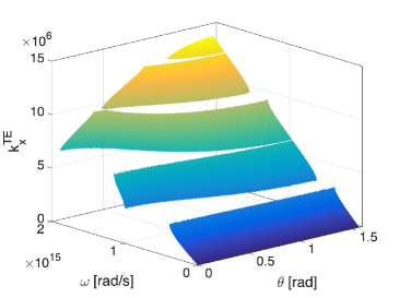
(c)

Figure 3: a) argument of $cos^{-1}$ in 17 for TE modes. Flat surfaces (red) at $\pm 1$ are added as a reference, b) regions with different Riemann sheets, and c) $k_{x}^{TE}$ after removing regions with imaginary $k_{x}^{TE}$ (band-gaps). The 1D PC parameters are $d_{1}=300\>nm,$ $d_{2}=700\>nm,$ $\varepsilon_{1}=11.9,$ $\varepsilon_{2}=2.1.$

Note that the inverse cosine function in (17) is a multi-valued function with branch cuts on positive and negative sides of the real axis ( $[-\infty,-1]$ and $[1,+\infty]$ segments). Every pass of the inverse cosine argument across a branch cut requires considering a different (appropriate) Riemann sheet. The argument of the $cos^{-1}$ function in (17) for TE modes of the 1D PC example discussed here is shown in Fig. (3). The crossing points of this function through branch cuts are where its $\frac{\partial}{\partial\omega}\left(.\right)=0.$ This leads to the Riemann sheet assignment shown in Fig. 5 (b) so that

$$cos^{-1}\left(x\right)=\begin{cases}\begin{array}[]{c}\left(n-1\right)\pi+\mathrm{P.V.}\\ n\pi-\mathrm{P.V.}\end{array}&\begin{array}[]{c}\mathrm{@Riemann}\;n,\quad\mathrm{for\>}\mathrm{odd\>n}\\ @\mathrm{Riemann}\;n,\quad\mathrm{for\>}\mathrm{even\>n}\end{array}\end{cases}$$ (23)

where P.V. is the principal value of $cos^{-1}\left(x\right)$ as $0\leq P.V.\leq\pi.$ The resulting $k_{x}^{TE}$ is also shown in Fig. 3.

Conclusion

The density of Bloch states inside a 1D PC was formulated based on its dispersion relations for both TE and TM modes. The quantities were calculated for a practical 1D PC in the visible range.

Appendix

The ratio of the radiation to absorption, $F\left(\omega,T\right),$ is considered to be a universal function for all solid matters based on Kirchhoff’s law (controversies regarding Kirchhoff’s law are beyond the purpose of this paper, see [7, 8] for details.) There are several methods to obtain $F\left(\omega,T\right),$ a.k.a. the black body radiation spectrum, inside a black body cavity. They all lead to

$$F\left(\omega,T\right)=\rho\left(\omega\right)U\left(\omega,T\right)$$ (24)

where $F\left(\omega,T\right)$ is considered to be a continuous function of $\omega$ with the unit of joules per frequency per volume ($\frac{J}{m^{3}Hz}$), and $U$ is the average total energy of the oscillators inside the black body (or photons in the cavity). In the state of thermal equilibrium, $U$ can be obtained either using the equipartition theorem in classical statistical mechanics ($U=kT,$ where $k$ is Boltzmann’s constant) leading to Rayleigh-Jeans distribution, or using Plank’s energy quantization arguments leading to

$$U=\hbar\omega/\left(exp(\frac{\hbar\omega}{kT})-1\right).$$ (25)

One of the most intuitive methods to obtain $\rho\left(\omega\right)$ in (24) (for isotropic homogeneous materials) is to count the supported electromagnetic modes inside the resonator in the interval $\left[\omega,\omega+d\omega\right]$, as we did in the main text. It can also be obtained from the emission by classical resonators into an unbounded isotropic medium (modeling a very large cavity) as follows [9]. Consider a particle with mass $m$ and charge $e$ acted upon by an elastic restoring force $-m\omega_{0}^{2}z$ and an external electric field of $E_{z}\left(t\right).$ For simplicity, assume the particle only moves in one dimension ($z$). Newton’s equation of motion for such particle is

$$\ddot{z}+\omega_{0}^{2}z=\frac{e}{m}E_{z}\left(t\right)+\frac{e}{m}E_{RR}\left(t\right)$$ (26)

where $E_{RR}\left(t\right)$ is the reaction electric field originated from the moving particle itself, and can be shown to be $E_{RR}\left(t\right)=\frac{2e}{3c^{3}}\dddot{z}\left(t\right).$ If the particle is inside a large rectangular cavity (with size L), the energy absorption rate by the particle oscillating with frequency $\omega_{0}$ from a cavity resonant mode at frequency $\omega$ is

$$\dot{W_{A}}=\frac{e^{2}}{2m}\frac{\gamma\omega^{4}E_{z}^{2}\left(\omega\right)}{\left(\omega^{2}-\omega_{0}^{2}\right)^{2}+\gamma^{2}\omega^{6}};\quad\gamma=\frac{2e^{2}}{3mc^{3}}$$ (27)

where $E_{z}\left(\omega\right)$ is the $z-$directed electric field associated with the electromagnetic mode, and $c$ is the speed of ($z-$polarized) light in the medium. If the radiation has a continuous broadband spectrum, with the (z-directed electric field) energy density of $F_{z}\left(\omega,T\right)d\omega=E_{z}^{2}\left(\omega\right)/\left(8\pi\right)$ in the interval $\left[\omega,\omega+d\omega\right]$, it can be shown that [9]

$$\dot{W_{A}}=\frac{4\pi e^{2}}{m}\intop_{\omega}\frac{\gamma F_{z}\left(\omega,T\right)d\omega}{\left(1-\omega_{0}^{2}/\omega^{2}\right)^{2}+\gamma^{2}\omega^{2}}.$$ (28)

For the frequencies of interest in thermal emissions, $\gamma\omega\ll 1$. If $F\left(\omega,T\right)$ is not sharply peaked, we may simplify (28) as

$$\dot{W_{A}}=\frac{4\pi e^{2}\gamma F_{z}\left(\omega_{0},T\right)}{m}\intop_{\omega}\frac{d\omega}{4\omega_{0}^{-2}\left(\omega-\omega_{0}\right)^{2}+\gamma^{2}\omega_{o}^{2}}$$ (29)

$$\qquad=\frac{4\pi e^{2}\gamma F_{z}\left(\omega_{0},T\right)}{m}\frac{\omega_{0}^{2}}{4}\frac{2\pi}{\gamma\omega_{0}^{2}}.$$

The energy emission rate of the oscillating charge is

$$\dot{W_{E}}=\frac{2e^{2}\omega_{0}^{2}}{3mc^{3}}U$$ (30)

where $c$ is the speed of light in vacuum, and $U$ is the average total oscillator energy. In the state of thermal equilibrium between the radiational energy and the matter, (30) and (29) should be equal, leading to

$$F\left(\omega_{0},T\right)=\frac{\omega_{0}^{2}}{\pi^{2}c^{3}}U,$$ (31)

where $F_{x}\left(\omega_{0},T\right)=F_{y}\left(\omega_{0},T\right)=F_{z}\left(\omega_{0},T\right)=F\left(\omega_{0},T\right)/3$ is used. Similar to the resonator mode counting method, (31) gives

$$\rho\left(\omega\right)=\frac{\omega^{2}}{\pi^{2}c^{3}}.$$ (32)

Also, equations (24), (25), and (32) provide the well-known Plank’s emission spectrum inside a blackbody cavity filled with an isotropic homogeneous material.

This method of obtaining $\rho\left(\omega\right)$ provides insight into how radiators inside the matter (e.g. blackbody) couple to the electromagnetic modes in common situations (leading to Plank’s radiation spectrum). Two critical assumptions which simplified (28) to (29) are 1) radiation spectrum, $F_{z}\left(\omega,T\right),$ does not have any sharp peaks, and 2) the resonators’ coupling to the radiation is sharply peaked around their natural frequency, $\omega_{0}.$ This assumption also implicitly requires linearity of the material. Only with these assumptions we obtained the same $\rho\left(\omega\right)$ as using the other, more fundamental, methods such as BE distribution of photons in the cavity in thermal equilibrium. It appears that (28) is a good starting point to study the thermal emission from non-linear (or any other uncommon) material.

References

• [1] G. Kirchhoff, “On the relation between the radiating and absorbing powers of different bodies for light and heat,” The London, Edinburgh, and Dublin Philosophical Magazine and Journal of Science, vol. 20, no. 130, pp. 1–21, 1860.
• [2] M. Planck, The theory of heat radiation.   Courier Corporation, 2013.
• [3] Reichl, Linda E. "A modern course in statistical physics." (1999): 1285-1287.
• [4] E. Forati, “Spontaneous emission rate and the density of states inside a one dimensional photonic crystal,” xx-arxiv, 2021.
• [5] L. Qi and C. Liu, “Complex band structures of 1d anisotropic graphene photonic crystal,” Photonics Research, vol. 5, no. 6, pp. 543–551, 2017.
• [6] J. Joannopoulos, R. Meade, and J. Winn, “Photonic crystals,” Molding the flow of light, 1995.
• [7] P.-M. Robitaille, “Kirchhoff’s law of thermal emission: 150 years,” Progr. Phys, vol. 4, pp. 3–13, 2009.
• [8] P.-M. Robitaille, “On the validity of Kirchhoff’s law of thermal emission,” IEEE transactions on plasma science, vol. 31, no. 6, pp. 1263–1267, 2003.
• [9] P. W. Milonni, The quantum vacuum: an introduction to quantum electrodynamics.   Academic press, 2013.