On The Absolute Constant in
Hanson-Wright Inequality

Abstract

We revisit and slightly modify the proof of the Gaussian Hanson-Wright inequality where we keep track of the absolute constant in its formulation.

In this short report we investigate the following concentration of measure inequality which is a special case of the Hanson-Wright inequality [1, 2]:

Theorem 1 (Gaussian Hanson-Wright Inequality).

Let $\underline{\boldsymbol{x}}\sim N(0,I_{n})$ be a standard Gaussian vector of length $n$. If $A$ is a nonzero $n\times n$ matrix, then

$$\Pr\big{(}|\underline{\boldsymbol{x}}^{T}A\underline{\boldsymbol{x}}-\mathbb{E}[\underline{\boldsymbol{x}}^{T}A\underline{\boldsymbol{x}}]|\geq a\big{)}\leq 2\exp\Big{(}-\kappa\min\Big{\{}\frac{a^{2}}{\|A\|_{2}^{2}},\frac{a}{\|A\|}\Big{\}}\Big{)},$$ (1)

for every $a>0$ where $\kappa$ is an absolute constant that does not depend on $n$, $A$ and $a$.

Here, $\|A\|_{2}$ is the Hilbert-Schmidt norm of $A$ defined by

$$\|A\|_{2}:=(\mathrm{tr}(A^{T}A))^{\frac{1}{2}}$$

and $\|A\|$ is the operator norm of $A$ given by

$$\|A\|:=\max_{\|\underline{x}\|_{2}\leq 1}\|A\underline{x}\|_{2}=(\lambda_{\max}(A^{T}A))^{\frac{1}{2}},$$

where $\lambda_{\max}(M)$ denotes the largest eigenvalue of a matrix $M$.

The largest value for $\kappa$ in (1) is unknown. Even a lower bound on $\kappa$ is not reported in the literature. The following proposition presents a value for $\kappa$ in the special case where the matrix $A$ in (1) is a real symmetric matrix:

Proposition 1.

For every $0<r<1$ define

$$\xi_{r}:=\sum_{k=0}^{\infty}\frac{r^{k}}{k+2}.$$ (2)

If the matrix $A$ in (1) is real symmetric, then one can let

$$\kappa=\frac{1}{4}\max_{0<r<1}\min\Big{\{}r,\frac{1}{2\xi_{r}}\Big{\}}.$$ (3)

Proof.

See the Appendix. ∎

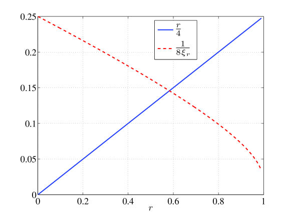
Figure 1: Plots of $\frac{r}{4}$ and $\frac{1}{8\xi_{r}}$ in terms of $0<r<1$. We see that $\min\{r,\frac{1}{2\xi_{r}}\}$ is maximized for $r\approx 0.583$ and its maximum value is approximately $0.1457$.

Fig. 1 shows plots of $\frac{r}{4}$ and $\frac{1}{8\xi_{r}}$ in terms of $0<r<1$. We see that $\frac{1}{4}\min\{r,\frac{1}{2\xi_{r}}\}\approx 0.1457$.

Appendix; Proof of Proposition 1

Since $A$ is real symmetric, we can write $A=U^{T}\Lambda U$ where $U$ is an orthogonal matrix and $\Lambda$ is a diagonal matrix with real diagonal entries $\lambda_{1},\cdots,\lambda_{n}$. Define $\boldsymbol{y}:=U\boldsymbol{x}$. Then $\boldsymbol{y}\sim\mathrm{N}(0,I_{n})$, $\boldsymbol{x}^{T}A\boldsymbol{x}=\sum_{i=1}^{n}\lambda_{i}\boldsymbol{y}_{i}^{2}$ and $\mathbb{E}[\boldsymbol{x}^{T}A\boldsymbol{x}]=\sum_{i=1}^{n}\lambda_{i}$. Fix $0<r<1$ and let

$$0<t\leq\frac{r}{2\max_{i}|\lambda_{i}|}$$ (4)

Applying Markov’s inequality [3],

$$\Pr(\boldsymbol{x}^{T}A\boldsymbol{x}-\mathbb{E}[\boldsymbol{x}^{T}A\boldsymbol{x}]>a) \leq e^{-ta}\prod_{i=1}^{n}\mathbb{E}[e^{t\lambda_{i}(\boldsymbol{y}_{i}^{2}-1)}]$$ (5)

$$= e^{-ta}\prod_{i=1}^{n}\mathbb{E}[e^{t\lambda_{i}(\boldsymbol{y}_{i}^{2}-1)}]$$

$$= e^{-ta}\prod_{i=1}^{n}\frac{e^{-t\lambda_{i}}}{\sqrt{1-2t\lambda_{i}}},$$

where the last step is due to $|t\lambda_{i}|<\frac{1}{2}$ and the fact that $\mathbb{E}[e^{s\boldsymbol{y}^{2}}]=(1-2s)^{-\frac{1}{2}}$ for any $s<\frac{1}{2}$ and $\boldsymbol{y}\sim\mathrm{N}(0,1)$. Let us write

$$\frac{1}{\sqrt{1-2t\lambda_{i}}} = e^{-\frac{1}{2}\ln(1-2t\lambda_{i})}$$ (6)

$$= e^{\frac{1}{2}\sum_{k=1}^{\infty}\frac{(2t\lambda_{i})^{k}}{k}}$$

$$= e^{t\lambda_{i}}e^{2t^{2}\lambda_{i}^{2}\sum_{k=0}^{\infty}\frac{(2t\lambda_{i})^{k}}{k+2}}$$

$$\leq e^{t\lambda_{i}}e^{2t^{2}\xi_{r}\lambda_{i}^{2}},$$

where the second step is due to $-\ln(1-x)=\sum_{k=1}^{\infty}\frac{x^{k}}{k}$ for any $|x|<1$, the last step is due to $2t|\lambda_{i}|\leq r$ and $\xi_{r}$ is defined in (2). By (5) and (6),

$$\Pr(\boldsymbol{x}^{T}A\boldsymbol{x}-\mathbb{E}[\boldsymbol{x}^{T}A\boldsymbol{x}]>a)\leq\exp\Big{(}-ta+2t^{2}\xi_{r}\sum_{i=1}^{n}\lambda_{i}^{2}\Big{)}.$$ (7)

Minimizing $-ta+2t^{2}\xi_{r}\sum_{i=1}^{n}\lambda^{2}_{i}$ in terms of $t$ subject to the constraint in (4), we get

$$t=\min\Big{\{}\frac{a}{4\xi_{r}\sum_{i=1}^{n}\lambda_{i}^{2}},\frac{r}{2\max_{i}|\lambda_{i}|}\Big{\}}.$$ (8)

If $\frac{r}{2\max_{i}|\lambda_{i}|}\leq\frac{a}{4\xi_{r}\sum_{i=1}^{n}\lambda_{i}^{2}}$, then $t=\frac{r}{2\max_{i}|\lambda_{i}|}$ and simple algebra shows that

$$-ta+2t^{2}\xi_{r}\sum_{i=1}^{n}\lambda_{i}^{2}\leq-\frac{ra}{4\max_{i}|\lambda_{i}|}.$$ (9)

If $\frac{r}{2\max_{i}|\lambda_{i}|}>\frac{a}{4\xi_{r}\sum_{i=1}^{n}\lambda_{i}^{2}}$, then $t=\frac{a}{4\xi_{r}\sum_{i=1}^{n}\lambda_{i}^{2}}$ and we get

$$-ta+2t^{2}\xi_{r}\sum_{i=1}^{n}\lambda^{2}_{i}=-\frac{a^{2}}{8\xi_{r}\sum_{i}\lambda_{i}^{2}}.$$ (10)

By (7), (9) and (10) and after replacing $\max_{i}|\lambda_{i}|$ and $\sum_{i=1}^{n}\lambda_{i}^{2}$ by $\|A\|$ and $\|A\|_{2}^{2}$, respectively,

$$\Pr(\boldsymbol{x}^{T}A\boldsymbol{x}-\mathbb{E}[\boldsymbol{x}^{T}A\boldsymbol{x}]>a)\leq\exp\Big{(}-\min\Big{\{}\frac{a^{2}}{8\xi_{r}\|A\|_{2}^{2}},\frac{ra}{4\|A\|}\Big{\}}\Big{)}.$$ (11)

Replacing the matrix $A$ by $-A$ and following the same lines of reasoning, we see that $\Pr(\boldsymbol{x}^{T}A\boldsymbol{x}-\mathbb{E}[\boldsymbol{x}^{T}A\boldsymbol{x}]<-a)$ is bounded from above by the same expression on the right side of (11). Hence,

$$\Pr(|\boldsymbol{x}^{T}A\boldsymbol{x}-\mathbb{E}[\boldsymbol{x}^{T}A\boldsymbol{x}]|>a) \leq 2\exp\Big{(}-\min\Big{\{}\frac{a^{2}}{8\xi_{r}\|A\|_{2}^{2}},\frac{ra}{4\|A\|}\Big{\}}\Big{)}$$ (12)

$$\leq 2\exp\Big{(}-\frac{1}{4}\min\Big{\{}r,\frac{1}{2\xi_{r}}\Big{\}}\min\Big{\{}\frac{a^{2}}{\|A\|_{2}^{2}},\frac{a}{\|A\|}\Big{\}}\Big{)}.$$

The upper bound in (12) holds for every $0<r<1$. Minimizing this bound over $r$, we get

$$\Pr(|\boldsymbol{x}^{T}A\boldsymbol{x}-\mathbb{E}[\boldsymbol{x}^{T}A\boldsymbol{x}]|>a)\leq 2\exp\Big{(}-\kappa\min\Big{\{}\frac{a^{2}}{\|A\|_{2}^{2}},\frac{a}{\|A\|}\Big{\}}\Big{)},$$ (13)

where $\kappa=\frac{1}{4}\max_{0<r<1}\min\big{\{}r,\frac{1}{2\xi_{r}}\big{\}}$.

References

• [1] D.Β L.Β Hanson and F.Β T.Β Wright, β€œA bound on tail probabilities for quadratic forms in independent random variables”, The Annals of Math. Statistics, vol.Β 42, no.Β 3, pp.Β 1079-1083, 1971.
• [2] M.Β Rudelson and R.Β Vershynin, β€œHanson-Wright inequality and sub-gaussian concentration”, Electronic Commun. in Probability, vol.Β 18, no.Β 82, pp.Β 1-9, 2013.
• [3] R. M. Dudley, β€œReal analysis and probability”, Cambridge University Press, 2002.
• [4] R.Β A.Β Horn and C.Β R.Β Johnson, β€œMatrix Analysis (2nd edition)”, Cambridge University Press, 2013.