Multidimensional self-trapping in linear and nonlinear potentials

Abstract

Solitons are typically stable objects in diverse one-dimensional (1D) models, but their straightforward extensions to 2D and 3D settings tend to be unstable. In particular, the ubiquitous nonlinear Schrödinger (NLS) equation with the cubic self-focusing, which is also widely known as the Gross-Pitaevskii (GP) equation in the theory of Bose-Einstein condensates (BECs), creates only unstable 2D and 3D solitons, because the same equation gives rise to destructive effects in the form of the critical and supercritical wave collapse in the 2D and 3D cases, respectively. This chapter offers, first, a review of physically relevant settings which, nevertheless, make it possible to create stable 2D and 3D solitons, including ones with embedded vorticity. The main stabilization schemes considered here are: (i) competing (e.g., cubic-quintic) and saturable nonlinearities; (2) linear and nonlinear trapping potentials; (3) the Lee-Huang-Yang correction to the mean-field BEC dynamics, leading to the formation of robust quantum droplets; (4) spin-orbit-coupling (SOC) effects in binary BEC; (5) emulation of SOC in nonlinear optical waveguides, including $\mathcal{PT}$-symmetric ones. Further, the chapter presents a detailed summary of results which demonstrate the creation of stable 2D and 3D solitons by the schemes based on the usual linear trapping potentials or effective nonlinear ones, which may be induced by means of spatial modulation of the local nonlinearity strength. The latter setting is especially promising, making it possible to use self-defocusing media, with the local nonlinearity strength growing fast enough from the center to periphery, for the creation of a great variety of stable multidimensional modes. In addition to fundamental states and vortex rings, the respective 3D modes may be hopfions, i.e., twisted vortex rings which carry two indpednent topological charges. Many results for the multidimensional solitons have been obtained, in such settings, not only in a numerical form, but also by means of analytical methods, such as the variational and Thomas-Fermi approximation.

Acronyms

1D – one-dimensional

2D – two-dimensional

3D – three-dimensional

a.r. – aspect ratio

b.c. – boundary condition(s)

BdG – Bogoliubov – de Gennes (linearized equations for perturbations around stationary solutions of GP/NLS equations)

BEC – Bose-Einstein condensate

CQ – cubic-quintic (nonlinearity))

CW – continuous wave

FR – Feshbach resonance

GP – Gross-Pitaevskii (equation)

GVD – group-velocity dispersion

HO – harmonic-oscillator (potential)

HV – hidden vorticity

IST inverse-scattering transform (the method for solving integrable nonlinear partial differential equations)

LHY – Lee-Huang-Yang (correction to the MF theory)

MF – mean-field (approximation)

NLS – nonlinear Schrödinger (equation))

OL – optical lattice

PDE – partial differential equation

PhR – photorefractive (optical material)

$\mathcal{PT}$ – parity-time (symmetry)

QD – quantum droplet

TF – Thomas-Fermi (approximation)

TS – Townes soliton

VA – variational approximation

VK – Vakhitov-Kolokolov (stability criterion)

XPM – cross-phase modulation

I Introduction: The objective of this chapter

Solitons, alias solitary waves, are self-trapped (localized) objects existing in a great variety of physical media, due to the interplay of basic linear properties, such as dispersion and/or diffraction, and nonlinearity which represents self-attraction of matter or fields that fill the media (Kivshar and Agrawal, 2003; Dauxois and Peyrard, 2006). Parallel to the development of experimental research of solitons in a large number of physical realizations, a great deal of work has been performed on theoretical models producing solitons (as it usually happens, the progress in the theoretical work was much faster). The theory has been developing in two related but distinct directions: on the one hand, elaboration of mathematical models of diverse physical setups, in which the concept of solitons is relevant, and, on the other hand, mathematical investigation of these and many other models (Zakharov et al., 1980; Ablowitz and Segur, 1981; Calogero and Degasperis, 1982; Newell, 1985; Takhtadjian and Faddeev, 1986; Yang, 2010). Actually, some models were introduced on the basis of their mathematical interest, rather than being directly suggested by physical realizations.

The concept of solitons and self-trapping had appeared in one-dimensional (1D) settings. Up to this day, an absolute majority of experimental and theoretical/mathematical studies of solitons have been performed in effectively 1D setups, and in the framework of 1D nonlinear partial differential equations (PDEs). The development of the studies for two- and three-dimensional (2D and 3D) systems, aimed at prediction and experimental creation of multidimensional solitons, is a fascinating possibility. However, a fundamental obstacle which strongly impedes the progress in this direction is the problem of stability of 2D and 3D solitons (Malomed et al., 2005 and 2016; Malomed, 2016; Mihalache, 2017; Kartashov et al., 2019; Malomed, 2019). In most cases, 1D solitons appear as fully stable solutions of the underlying PDEs, and they are readily observed as stable objects in the experiment. On the other hand, the ubiquitous NLS equation with the cubic self-focusing nonlinearity creates only unstable solitons in 2D and 3D spaces, because precisely the same equations gives rise to the phenomena of the wave collapse (alias blowup), i.e., spontaneous formation of singularities in finite times, starting from regular localized (soliton-like) inputs. The collapse governed by the cubic NLS equation is critical in the 2D geometry, i.e., it sets in if the integral norm of the input exceeds a certain critical value; otherwise, the input spreads out. In 3D, the same equation gives rise to the supercritical collapse, for which the threshold value of the norm is zero, i.e., the formation of the singularity may be initiated by the input with an arbitrarily small norm. In either case, the possibility of the collapse makes the formally existing 2D and 3D soliton solutions of the NLS equation completely unstable.

For this reason, the cardinal direction in the work on the vast area of self-trapping in the multidimensional geometry has been elaboration of physically relevant setups in which 3D and 3D solitons may be stabilized (Malomed et al., 2005 and 2016; Malomed, 2016; Mihalache, 2017; Kartashov et al., 2019; Malomed, 2019). One of promising directions is the use of trapping potentials. First of all, this may be a straightforward linear potential, such as the parabolic (alias harmonic-oscillator (OH) one). A more sophisticated option is the use of self-repulsive nonlinearity with a spatially modulate strength of the local interaction. While, in the uniform space, the self-repulsion obviously cannot give rise to self-trapping, it can readily support a remarkable variety of stable 1D, 2D, and 3D localized states (quasi-solitons), provided that the local strength of the self-repulsion in the space of dimension $D$ grows fast enough from the center to periphery (faster than $r^{D}$, where $r$ is the radial coordinate), as was first proposed by Borovkova et al. (2011a,2011b) and later developed in many other works, see below. The latter setup may be considered as one with an effective nonlinear potential.

The objective of this chapter is to provide a summary of theoretical results obtained on this topic, including a review of diverse methods elaborated for the stabilization of multidimensional solitons in systems of the NLS type, and a detailed account of theoretical results predicting stable 2D and 3D solitons in the framework of the NLS equation including linear or nonlinear potentials. The presentation is arranged as follows. To provide the necessary introduction to the general topic, Section II recapitulates basic results which were firmly established in studies of integrable and non-integrable versions of the one-dimensional NLS equations. Section III leads the reader from 1D to the multidimensional world. In particular, it introduces a concept of the Townes solitons (TSs), which are unstable, by themselves, are closely related to various stabilization schemes, and outlines the fundamental problem of the instability of NLS solitons in the multidimensional space. Section IV provides a summary of basic stabilization schemes, elaborated for the 2D and 3D solitons in systems of the NLS types. Sections V and VI summarize essential predictions for the existence of stable fundamental solitons, as well as topologically structured ones, such as 2D and 3D vortex rings and 3D hopfions (twisted vortex rings), in models including, respectively, linear or nonlinear potentials as the stabilizing factor. Section VII concludes the chapter.

II The one-dimensional NLS (nonlinear Schrödinger) equation – a universal model of classical and semi-classical physics

II.1 The general setting

The great amount of work performed on PDEs modeling the wave propagation in 1D dispersive nonlinear media had led, roughly 50 years ago, to the discovery of several celebrated equations, which are fundamentally important as universal models of the theory of nonlinear waves. These equations share the unique property of integrability, which was revealed with the help of the mathematical technique known as the inverse-scattering transform (IST). Three most important items in the list of classical integrable PDEs are the Korteweg - de Vries (KdV), sine-Gordon (SG), and nonlinear Schrödinger (NLS) equations. Methods for solving these equations and results produced by those methods are summarized, in full detail, in several well-known books (Zakharov et al., 1980; Ablowitz and Segur, 1981; Calogero and Degasperis, 1982; Newell, 1985; Takhtadjian and Faddeev, 1986; Rogers and Schief, 2002; Yang. 2010).

The NLS equation plays the central role in the present chapter. In 1D, its scaled form is commonly known:

$$i\psi_{z}+\frac{1}{2}\psi_{xx}\pm|\psi|^{2}\psi-U(x)\psi=0.$$ (1)

This equation is commonly used as the model for the propagation of light, with local amplitude $\psi\left(x,z\right)$ of the electromagnetic field, in planar optical waveguides with transverse coordinate $x$ and propagation distance $z$ (Kivshar and Agrawal, 2003). In this case, term $\psi_{xx}$ represents the paraxial diffraction, the cubic term with the top or bottom signs corresponds, respectively, to the self-focusing or defocusing Kerr nonlinearity in the waveguiding material, and $-U(x)$ is proportional to the local variation of the underlying refractive index, $\delta n\left(x\right)$. On the other hand, Eq. (2.1) with $z$ replaced by scaled time $t$ is well known as the semi-classical Gross-Pitaevskii (GP) equation for the mean-field wave function, $\psi\left(x,t\right)$, of a Bose-Einstein condensate (BEC) of ultracold bosonic atoms loaded into a tightly built cigar-shaped trapping potential, which effectively eliminates the transverse coordinates ($y$ and $z$), allowing BEC to evolve in time along the axial direction, $x$ (Pitaevskii and Stringari, 2003). In this case, the top and bottom signs in front of the cubic term in Eq. (2.1) imply, respectively, attractive and repulsive interactions between atoms in the ultracold gas, and a real axial potential, $U(x)$, is an essential ingredient of experimental setups. The potential which is often used in the experiment represents the harmonic oscillator (HO),

$$U_{\mathrm{OH}}(x)=\left(\Omega^{2}/2\right)x^{2}.$$ (2)

Equation (2.1) for the complex wave function $\psi(x)$ corresponds to the Hamiltonian, which is considered as a functional of $\psi(x)$ and $\psi^{\ast}(x)$, where $\ast$ stands for the complex conjugate function:

$$H=\int_{-\infty}^{+\infty}\left[\frac{1}{2}\left|\psi_{x}\right|^{2}+U(x)|\psi|^{2}\mp\frac{1}{2}|\psi|^{4}\right]dx.$$ (3)

The NLS equation can be written in terms of the Hamiltonian in the standard form (Takhtadjian and Faddeev, 1986),

$$\frac{\partial\psi}{\partial z}=-i\frac{\delta H}{\delta\psi^{\ast}},$$ (4)

where $\delta/\delta\psi^{\ast}$ stands for variational (Freché) derivative, and the application of the derivative makes use of the identities $\left|\psi(x)\right|^{2}\equiv\psi(x)\psi^{\ast}(x)$ and $\left|\psi_{x}\right|^{2}\equiv\psi_{x}\psi_{x}^{\ast}$. In the presence of real potential $U(x)$, the non-integrable equation (2.1) conserves two dynamical invariants: the total norm (alias the integral power, in terms of the optical realization),

$$N=\int_{-\infty}^{+\infty}\left|\psi(x)\right|^{2}dx,$$ (5)

and the Hamiltonian.

II.2 The integrable NLS equation

NLS equation (2.1) is integrable in the free space, with $U(x)=0$ (it is also integrable in the case of a linear potential, $U(x)=Cx$, as this potential may be eliminated from Eq. (2.1) by means of a gauge transformation (Chen and Liu, 1976)). In the case of the top sign in front of the cubic term (the self-focusing), the family of bright-soliton solutions to this equation, with arbitrary amplitude $\eta$ and velocity $c$, is commonly known since it was obtained in the same classical work of Zakharov and Shabat (1971), in which the integrability of Eq. (2.1) with $U(x)=0$ was discovered:

$$\psi_{\mathrm{sol}}^{\mathrm{(1D)}}\left(x,t\right)=\eta~{}\mathrm{sech}\left(\eta(x-cz)\right)\exp\left(icx+ik_{\mathrm{sol}}z\right).$$ (6)

Here, the soliton’s propagation constant is

$$k_{\mathrm{sol}}=\frac{1}{2}\left(\eta^{2}-c^{2}\right).$$ (7)

In terms of the above-mentioned optics realization, this solution produces a spatial (stripe) soliton, $c$ actually being not the velocity, but the slope of soliton’s stripe in the $\left(x,z\right)$ plane. The profile of soliton (2.6) with $\eta=1$ and $c=0$ is displayed in Fig. 1(a).

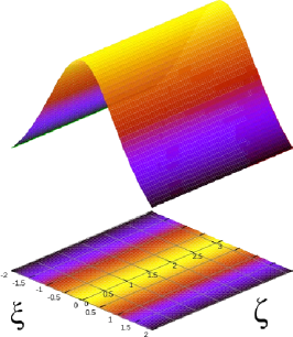
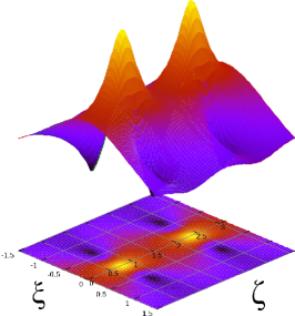
Figure 1: (a) The profile of the absolute value of the wave field, $\left|\psi\left(x\equiv\xi,z\equiv\zeta\right)\right|$, and its projection onto the $\left(\xi,\zeta\right)$ plane, which represents the fundamental bright-soliton solution (2.6) with $\eta=1$ and $c=0$. (b) The same for the second-order breather (two-soliton), which is produced by input (2.10) with $\mathcal{N}=2$ (source: Wikipedia, creator: Alessio Damato, https://commons.wikimedia.org/wiki/File:Soliton_1st_order.svg#filelinks).

The free-space NLS equation (not necessarily Eq. (2.1), but also ones with a more general nonlinearity, which are not integrable) conserves the total momentum,

$$P=i\int_{-\infty}^{+\infty}\psi\psi_{x}^{\ast}dx.$$ (8)

Integrable systems, such as Eq. (2.1) with $U(x)=0$, conserve an infinite set of higher-order dynamical invariants, in addition to the three lowest ones, $N$, $P$, and $H$, but they do not have a straightforward physical meaning. For the fundamental bright-soliton solution (2.6), values of the basic conserved quantities are

$$N_{\mathrm{sol}}=2\eta,P_{\mathrm{sol}}=2c\eta,H_{\mathrm{sol}}=-\frac{1}{3}\eta^{3}+\eta c^{2}.$$ (9)

The integrability of the NLS equation makes it possible to construct exact solutions for collisions of solitons moving with different velocities (or different spatial slopes, in terms of the spatial-domain light propagation in the planar waveguide), $c_{1}$ and $c_{2}$. A well-known result is that the collisions are fully elastic, i.e., the solitons reappear from the collisions with precisely the same shapes, amplitudes, and velocities which they had originally. The only effect produced by the collision is the shift of both solitons along coordinate $x$, and a shift of their intrinsic phases. In particular, solitons with equal amplitudes $\eta$, colliding with velocities $\pm c$, shift in the direction of their motion by $\Delta x=\pm\eta^{-1}\ln\left(1+4\eta^{2}/c^{2}\right)$.

Another important manifestation of the integrability of the NLS equation (2.1) in the free space ($U(x)=0$) with the top sign was discovered by Satsuma and Yajima (1974): the IST technique gives rise to highly nontrivial exact solutions in the form of $\mathcal{N}$-solitons, produced by the initial condition

$$\psi(x,z=0)=\mathcal{N}\,\mathrm{sech}\,x$$ (10)

with integer $\mathcal{N}$. These states may be considered as nonlinear superpositions of $\mathcal{N}$ solitons with amplitudes $\eta=\left\{1,3,...,2\mathcal{N}-1\right\}$. Although the binding energy of such $\mathcal{N}$-soliton complexes is exactly equal to zero, the solitons stay together, forming an oscillatory state, which is often called a breather. This solution can be written in a relatively simple form for $\mathcal{N}=2$:

$$\psi_{\mathrm{two-sol}}\left(x,t\right)=4e^{iz/2}\frac{\cosh\left(3x\right)+3e^{4iz}\cosh x}{\cosh\left(4x\right)+4\cosh\left(2x\right)+3\cos\left(4z\right)}.$$ (11)

As shown in Fig. 1(b), the two-soliton breather, given by Eq. (2.11), periodically oscillates between broad and narrow shapes, the latter one featuring a single central peak and two small side peaks. For $\mathcal{N}=3$ in Eq. (2.10), the analytical form of the resulting three-soliton solution is cumbersome, while its spatiotemporal evolution, displayed in Fig. 2(a), along with the respective Fourier transform in Fig. 2(b), exhibit a new feature, in comparison with the two-soliton breather: the central peak periodically splits in two, which then recombine back. Only very recently such a third-order soliton (breather) was observed experimentally in BEC (Luo et al., 2020).

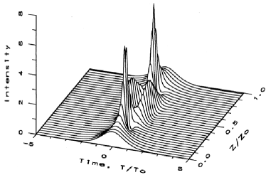
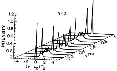
Figure 2: The profile of the local intensity of the wave field, $\left|\psi\right|^{2}$, in the coordinate domain (a), and the intensity of its Fourier transform (b), for the three-soliton (third-order breather), generated by input (2.10) with $\mathcal{N}=3$. Note that the central peak of the breather periodically splits in two secondary peaks, which then recombine back into the single one. The evolution variable is denoted $z$, corresponding to the propagation distance in fiber optics (source: the book by Agrawal (2013).

The input in the form given by Eq. (2.10) is relevant in the general case too, when $\mathcal{N}$ is not an integer. In this case, an explicit solution for $\psi\left(x,t\right)$ is not available, but the respective set of scattering data, in terms of the IST method, was also found in an exact form by Satsuma and Yajima (1974). The set contains a higher-order soliton (breather) of order $\mathcal{N}_{\mathrm{sol}}=\left[\mathcal{N}+1/2\right]$ (with $\left[...\right]$ standing for the integer part), “contaminated” by a dispersive radiation component. In particular, input (2.10) with $1/2<\mathcal{N}<3/2$ creates the output containing exactly one soliton (2.6) mixed with the radiation field.

The NLS equation (2.1) with $U(x)=0$ and the bottom sign in front of the cubic term, which represents the self-defocusing nonlinearity, gives rise to dark solitons, supported by the continuous-wave (CW) background with nonzero intensity $\left|\psi\right|^{2}\equiv n_{0}$ at $|x|\rightarrow\infty$. In terms of optics, dark solitons represent a dark spot on top of the uniformly lit backdrop:

$$\psi_{\mathrm{dark}}\left(x,z\right)=\exp\left(in_{0}z\right)\left\{\sqrt{n_{0}-c^{2}}\tanh\left(\sqrt{n_{0}-c^{2}}\left(x-cz\right)\right)+ic\right\}.$$ (12)

In the case of $c=0$, the dark-soliton’s field (2.6’) vanishes at $x=0$. The solution with positive or negative speed $c$, subject to constraint $|c|<\sqrt{n_{0}}$, represents the dark soliton moving across the background with this speed (moving dark solitons are usually called gray solitons).

Both the bright and dark solitons are completely stable solutions of the respective NLS equation (2.1). In particular, their stability agrees with the necessary (but, generally speaking, not sufficient) condition for the stability of solitons supported by the self-attractive nonlinearity, known as the Vakhitov-Kolokolov (VK) stability criterion (Vakhitov and Kolokolov, 1973; this fundamentally significant criterion is considered in detail in reviews of Bergé (1998) and Zakharov and Kuznetsov (2012), and in the book of Fibich (2015)). The VK criterion is written for the norm of the soliton family, considered as a function of the chemical potential:

$$dN/dk>0.$$ (13)

Indeed, it is obvious that the NLS-soliton’s norm, given by Eq. (2.9), if considered as a function of the chemical potential as per Eq. (2.7), i.e., $N_{\mathrm{sol}}=2\sqrt{2k_{\mathrm{sol}}}$ satisfies condition (2.12). Here, this point is considered for the zero soliton’s velocity, $c=0$, because the velocity does not affect the stability of solutions of Galilean-invariant equations, Eq. (2.1) with $U(x)=0$ being one of them. Indeed, any quiescent solution of Eq. (2.1) generates a family of moving ones, with velocity $c$, by means of the Galilean boost:

$$\psi\left(x,z\right)_{c\neq 0}=\psi\left(x,z\right)_{c=0}\left(x-cz,z\right)\exp\left(icx+\frac{i}{2}c^{2}z\right).$$ (14)

Moreover, the bright soliton realizes the ground state of the NLS-based setup, i.e., it is the state with the lowest value of Hamiltonian (2.3) for fixed norm (2.5) (Zakharov and Kuznetsov, 2012). The simplest way to arrive at this conclusion is to consider an ansatz for the stationary wave function,

$$\left|\psi(x)\right|=A^{2}\,\mathrm{sech}\left(x/W\right),$$ (15)

with amplitude $A$ and width $W$. The norm (2.5) of the ansatz is

$$N=2A^{2}W.$$ (16)

Then, following the principle of the variational approximation (VA) (Anderson and Bonnedal, 1979; Anderson, 1983; Malomed, 2002), one calculates the value of Hamiltonian (2.3) for the ansatz (2.14), with $A^{2}$ expressed in terms of $N$ as per Eq. (2.15):

$$H_{\mathrm{ans}}=\frac{1}{6}\left(\frac{N}{W^{2}}-\frac{N^{2}}{W}\right).$$ (17)

Finally, the minimization of this expression identifies the width of the ground state, $W=2/N$, which exactly corresponds to the exact bright-soliton solution (2.6).

II.3 An example of exact solitons in a non-integrable NLS equation with the delta-functional trapping potential

To gain insight into families of NLS solitons in a non-integrable version of the NLS equation, on can Eq. (2.1), with trapping potential $U(x)=-\varepsilon\delta(x)$, in which rescaling makes it possible to fix $\varepsilon=1$, both signs in front of the nonlinear term, and, moreover, with a more general power of the nonlinearity, viz., $2\sigma+1$:

$$i\psi_{z}+\frac{1}{2}\psi_{xx}\pm|\psi|^{2\sigma+1}\psi+\delta(x)\psi=0.$$ (18)

It is easy to find exact solutions for solitons pinned to the trapping center (Wang, Malomed, and Yan, 2019):

$$\psi(x)=e^{ikz}\left[\sqrt{k(\sigma+1)}\,\mathrm{sech}\left(\sigma\sqrt{2k}\,(|x|+\xi)\right)\right]^{1/\sigma},$$ (19)

with a real positive constant

$$\xi=\left(2\sigma\sqrt{2k}\right)^{-1}\ln\left(\frac{\sqrt{2k}+1}{\sqrt{2k}-1}\right).$$ (20)

The squared amplitude of the pinned soliton is

$$A^{2}(\sigma,k)\equiv\left|\psi(x=0)\right|^{2}=\left[\left(1+\sigma\right)\left(k-1/2\right)\right]^{1/\sigma}.$$ (21)

It follows from Eqs. (2.18) and (2.19) that the solutions exist with the propagation constant exceeding a cutoff value,

$$k>k_{\mathrm{cutoff}}\equiv 1/2,$$ (22)

the amplitude vanishing at $k\rightarrow 1/2$.

The norm of solution (2.19) can be explicitly calculated for the cubic nonlinearity, with $\sigma=1$,

$$N_{\sigma=1}(k)=2\left(\sqrt{2k}-1\right),$$ (23)

and for the quintic nonlinearity, with $\sigma=2$:

$$N_{\sigma=2}(k)=\sqrt{\frac{3}{2}}\left[\pi-2\tan^{-1}\left(\sqrt{\frac{\sqrt{2k}+1}{\sqrt{2k}-1}}\right)\right].$$ (24)

Note that the norm given by Eq. (2.21) for $\sigma=1$ diverges at $k\rightarrow\infty$, while in the case of $\sigma=2$, which is the critical one in the 1D setting, the value given by Eq. (2.22) at $k\rightarrow\infty$ is finite:

$$N_{\sigma=2}(k\rightarrow\infty)=\sqrt{3}\pi\left(2\sqrt{2}\right)^{-1}\approx 1.92.$$ (25)

Accordingly, there is a discontinuity in the dependence of $N_{\sigma}(k\rightarrow\infty)$ on $\sigma$. First, it diverges in the subcritical case, $\sigma<2$ – in particular, as

$$N_{\sigma<2}(k)\approx\sqrt{3}\pi\left(2\sqrt{2}\right)^{-1}k^{\left(2-\sigma\right)/4}$$ (26)

for $0<2-\sigma\ll 2$. Next, it takes the final value (2.23) in the critical case, $\sigma=2$. Finally, $N(k\rightarrow\infty)$ decays $\sim k^{-(\sigma-2)/4}$ in the supercritical case, $\sigma>2$.

Dependences $N(k)$ for $\sigma\leq 2$, including the explicitly found ones, given by Eqs. (2.21) and (2.22), satisfy the VK criterion (2.12) at all values of $k>1/2$, at which the solitons exist. In full agreement with the prediction of the criterion, all soliton families (2.17) are fully stable at $\sigma\leq 2$ (Wang, Malomed, and Yan, 2019). In the supercritical case, $\sigma>2$, the family (2.17) satisfies the VK criterion in a finite interval of the propagation constant, which can be explicitly found for $0<\sigma-2\ll 1$:

$$\frac{1}{2}<k<k_{\mathrm{cr}}(\sigma)\approx\frac{8}{\left(\pi(\sigma-2)\right)^{2}}.$$ (27)

A narrow stability interval exists even in the limit of $\sigma\gg 2$, with $k_{\mathrm{cr}}(\sigma)-1/2\approx 1/\sigma$. In terms of the norm, the stability interval has a finite size too,

$$0<N<N_{\max}(\sigma)\equiv N_{\sigma}\left(k=k_{\mathrm{cr}}(\sigma)\right).$$ (28)

In particular, $N_{\max}\left(\sigma=2\right)$ is given by Eq. (2.23), and with the growth of $\sigma$, $N_{\max}(\sigma$) monotonously decreases towards $N_{\max}\left(\sigma\rightarrow\infty\right)=1$.

At $\sigma>2$ and $k>k_{\mathrm{cr}}(\sigma)$, the pinned solitons are unstable. These results, produced by means of the numerical solution of the stationary version of Eq. (2.16) with the upper sign, are summarized in Fig. 3).

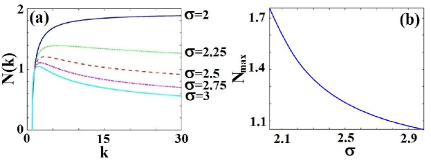
Figure 3: (a) The dependence of norm $N_{\sigma}(k)$ on propagation constant $k$, numerically computed from Eq. (2.16) with the top sign in front o the nonlinear term, for $\sigma=2$, and supercritical values, $\sigma=\ 2.25,\,2.5,\,2.75,\,3$. According to the VK criterion, the stability interval is one with $dN/dk>0$. (b) The maximum norm of the pinned solitons, defined as per Eq. (2.26), versus $\sigma$  in the supercritical interval, $2<\sigma\leq 3$. The figure is borrowed from the paper by Wang, Malomed, and Yan (2019).

In addition to that, it is possible to produce a family of exact solutions for solitons pinned to the attractive delta-functional potential in the case of the self-repulsive nonlinearity, corresponding to the top sign in Eq. (2.16) (Wang, Malomed, and Yan, 2019):

$$\psi_{\mathrm{defoc}}(x)=e^{-kz}\left\{\sqrt{k(\sigma+1)}/\sinh\left[\sigma\sqrt{2k}\,(|x|+\xi)\right]\right\}^{1/\sigma},$$ (29)

with

$$\xi=\frac{1}{2\sigma\sqrt{2k}}\ln\left(\frac{1+\sqrt{2k}}{1-\sqrt{2k}}\right),$$ (30)

and the squared amplitude

$$A^{2}(\sigma,k)\equiv\left|\psi_{\mathrm{defoc}}(x)\right|^{2}=\left[\left(1+\sigma\right)\left(1/2-k\right)\right]^{1/\sigma},$$ (31)

cf. the solution given by Eqs. (2.17) - (2.19). As it follows from Eqs. (2.28), the existence region for the localized modes pinned by the attractive delta-functional potential embedded in the defocusing medium is $k<k_{\mathrm{cutoff}}\equiv 1/2$, which is exactly opposite to that in the case of the self-focusing, cf. Eq. (2.20). As for the $N(k)$ dependence for these solutions, it takes a simple form in the case of the cubic self-repulsion, $\sigma=1$:

$$N_{\mathrm{defoc}}(\sigma=1,k)=2\left(1-\sqrt{2k}\right),$$ (32)

cf. dependence (2.21) for $\sigma=1$ in the case of the cubic self-attraction.

For localized states supported by self-repulsive nonlinearity, the VK criterion, as the necessary stability condition, is replaced by the anti-VK criterion, with the opposite sign (Sakaguchi and Malomed, 2010):

$$dN/dk<0,$$ (33)

cf. Eq. (2.12). The consideration demonstrates that the solutions given by Eqs. (2.27) and (2.28) satisfy the anti-VK criterion at all values of $\sigma$ and $k$ (see, e.g., Eq. (2.30)). Accordingly, the full stability analysis has demonstrated that all these solutions are indeed stable (Wang, Malomed, and Yan, 2019).

III The exit to the multidimensional world

III.1 Two-dimensional Townes solitons (TSs)

While there are important setups which make it possible to introduce physically relevant 1D systems, as briefly mentioned above, the real world is three-dimensional, and, in some cases, quasi-two-dimensional. This obvious fact strongly suggests to consider 3D and 2D solitons in nonlinear optics, BEC, plasmas, and other nonlinear physical media.

The simplest relevant model which admits direct extension from 1D to 3D and 2D is the cubic NLS/GP equation (in fact, as mentioned above, its 1D version (2.1) was derived by the inverse reduction, 3D $\rightarrow$ 1D):

$$i\psi_{t}+\frac{1}{2}\nabla^{2}\psi\pm|\psi|^{2}\psi-U(r)\psi=0,$$ (34)

where $\nabla^{2}$ is the 3D or 2D Laplacian, the top and bottom signs in front of the cubic term again correspond to the attractive and repulsive nonlinearity, respectively, and the trapping potential, if any, is assumed to be isotropic, depending on the radial coordinate,

$$r=\sqrt{x^{2}+y^{2}+z^{2}}$$ (35)

(or $r=\sqrt{x^{2}+y^{2}}$ in 2D). The Hamiltonian corresponding to Eq. (3.1) is

$$H=\frac{1}{2}\int\left(|\nabla\psi|^{2}-|\psi|^{4}\right)d^{D}x,$$ (36)

where $\int d^{D}x$ stands for the integration in the 3D or 2D space.

Equation (3.1) is written as the GP equation for the three-dimensional BEC. In the realization of the NLS equation as the spatiotemporal propagation equation in optics, the evolutional variable $t$ in Eq. (3.1) is replaced (as in Eq. (2.1)) by the propagation distance, $z$, while one of transverse coordinates is replaced by the local time, $\tau\equiv t-x/V_{\mathrm{gr}}$ (Kivshar and Agrawal, 2003), while two other spatial variables, $\left(x,y\right)$, keep the meaning of the transverse coordinates in the bulk optical waveguide.

In the multidimensional form, the GP/NLS equation (3.1) is always non-integrable. Powerful numerical methods have been developed for the solution of equations of this type, see reviews by Bao, Jaksch, and Markowich, 2003; Muruganandam and Adhikari, 2009; Vudragović et al., 2012; Bao and Cai, 2013. In particular, the ground state of many settings modeled by the GP equation can be looked for by means of the imaginary-time-integration (alias gradient-flow) method (Bao and Du, 2004). In spite of the complexity of the multidimensional nonlinear GP/NLS equations, in many cases analytical methods, such as the variational and Thomas-Fermi (TF) approximations, can be applied efficiently to these models, as shown, in particular, in sections V and VI of this chapter. In exceptional cases, exact analytical solutions can be found too (see, e.g., Eq. (6.15) below).

Fundamental (isotropic) localized solutions of Eq. (3.1) are looked for in the usual form,

$$\psi\left(r,t\right)=e^{-i\mu t}\phi(r),$$ (37)

where $\mu<0$ is a real chemical potential in the case of BEC ($-\mu$ is the propagation constant in the optics model), $r$ is the radial coordinate, and real function $\phi(r)$ obeys the equation

$$\mu\phi+\frac{1}{2}\left(\frac{d^{2}\phi}{dr^{2}}+\frac{D-1}{r}\frac{d\phi}{dr}\right)+\phi^{3}=0,$$ (38)

where $D=2$ or $3$ is the spatial dimension. Obviously, localized solutions of Eq. (3.5) have the asymptotic form

$$\phi(r)\sim r^{-(D-1)/2}\exp\left(-\sqrt{-2\mu}r\right).$$ (39)

Furthermore, in the 2D case the ansatz

$$\psi\left(r,\theta,t\right)=e^{-i\mu t+iS\theta}\phi_{S}(r),$$ (40)

where $\theta$ is the azimuthal coordinate, gives rise to 2D solitons with embedded integer vorticity (alias the winding number) $S=\pm 1,\pm 2$, … (Kruglov and Vlasov, 1985; Kruglov et al., 1988). In this case, Eq. (3.5) for real function $\phi_{S}(r)$ is replaced by

$$\mu\phi_{S}+\frac{1}{2}\left(\frac{d^{2}\phi_{S}}{dr^{2}}+\frac{1}{r}\frac{d\phi_{S}}{dr}-\frac{S^{2}}{r^{2}}\phi_{S}\right)+\phi_{S}^{3}=0.$$ (41)

The asymptotic form of relevant solutions to Eq. (3.8) at $r\rightarrow 0$ is obvious too:

$$\phi_{S}(r)\sim r^{|S|}.$$ (42)

The presence of the inner hole in the middle of the soliton, represented by Eq. (3.9), lends the vortex solitons an annular (ring-like) shape (see Fig. 13 below, which shows the hole in a 3D soliton with embedded vorticity).

The stationary equations (3.5) and (3.8) are invariant with respect to the conformal transformation,

$$\tilde{\mu}=l^{-2}\mu,\tilde{r}=lr,\tilde{\phi}=l^{-1}\phi,$$ (43)

which entails rescaling of the integral norm,

$$\tilde{N}=l^{D-2}N\equiv l^{D-2}\int|\psi|^{2}d^{D}x,$$ (44)

where $l$ is an arbitrary scaling factor. Thus, the norm of the 2D solitons with any vorticity $S$ is invariant with respect to the conformal transformation – in other words, for the soliton family with given $|S|$, the norm takes a single value, which does not depend on $\mu$.

In particular, for the 2D fundamental ($S=0$) NLS solitons, which are often called Townes solitons (TSs), which were first theoretically considered by Chiao, Garmire, and Townes (1964), this universal value is

$$N_{\mathrm{TS}}\approx 5.85.$$ (45)

An analytical approximation for the same value was elaborated by Desaix, Anderson, and Lisak (1991), who used the VA based on the Gaussian ansatz:

$$\left(N_{\mathrm{TS}}\right)_{\mathrm{VA}}=2\pi,$$ (46)

thus the relative inaccuracy of the VA is $\approx 7\%$. A numerically found plot of the TS is shown (in the Cartesian coordinates) in Fig. 4(a).

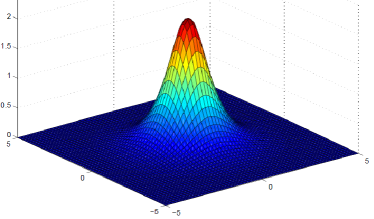
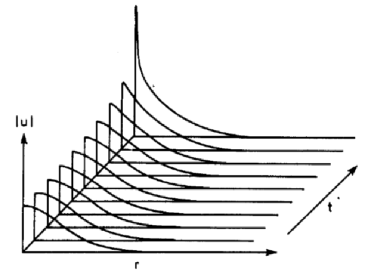
Figure 4: (a) A numerically found spatial profile of the two-dimensional TS (Townes soliton). (b) Development of the TS’s collapse shown in a radial cross-section (source: https://www2.mathematik.uni-halle.de/dohnal/SOLIT_WAVES/NLS_blowup.pdf).

As a matter of fact, the TSs were introduced by Chiao, Garmire, and Townes (1964) as the first example of solitons ever considered in optics (under the name of the “self-trapped optical beam”, as this happened before the term “soliton” was coined by Zabusky and Kruskal (1965)). However, the TSs are problematic objects, because they are subject to intrinsic instability, as shown below (nevertheless, weakly unstable TSs were recently created and observed in BEC, see Fig. 5 below).

The same argument which leads to Eqs. (3.11) and (3.12), i.e., the conclusion that the norm of the fundamental TSs does not depend on their size (or chemical potential), applies to the TSs with embedded vorticity, which were introduced, as mentioned above by Kruglov and Vlasov (1985), and Kruglov et al. (1988). At $S\geq 1$, the constant value of the norm grows nearly linearly with $S$, see an approximate analytical result for that, given below by Eq. (5.11).

III.2 Similarities: one- and three-dimensional Townes solitons (TSs)

It is relevant to mention that TSs can be defined in 1D as well as (Abdullaev and Salerno, 2005), as solutions to the 1D NLS equation with the self-attractive quintic term:

$$i\psi_{t}+\frac{1}{2}\psi_{xx}+|\psi|^{4}\psi=0,$$ (47)

with Hamiltonian

$$H=\int_{-\infty}^{+\infty}\left(\frac{1}{2}\left|\psi_{x}\right|^{2}-\frac{1}{3}|\psi|^{6}\right)dx,$$ (48)

cf. Eqs. (2.3) and (3.3). It admits a family of exact solutions in the form of

$$\psi_{\mathrm{TS}}^{\mathrm{(1D)}}=e^{-i\mu t}\frac{\left(-3/2\mu\right)^{1/4}}{\sqrt{\cosh\left(2\sqrt{-\mu}x\right)}},$$ (49)

which exist for all $\mu<0$. Actually, this solution coincides with the one given by Eq. (2.17) with $\xi=0$ (i.e., in the absence of the $\delta(x)$ term in Eq. (2.16)), in the case of $\sigma=2$, which was determined as the critical one in the above consideration.

As well as their 2D counterparts, the entire family of these TSs has the single value of the norm, which is identical to the one given above by Eq. (2.23). Recall that the solitons produced by the same equation including the $\delta$-functional potential term, i.e., solutions of Eq. (2.16) with the top sign in front of the nonlinear term with $\sigma=2$, which are given by expressions (2.16) and (2.17), are completely stable. On the contrary to that, all solitons (3.16) are unstable. It is relevant to mention that the substitution of solution (3.16) in expression (3.15) shows that the value of the Hamiltonian (energy) for the entire family of the one-dimensional TSs is exactly equal to zero:

$$H_{\mathrm{TS}}^{\mathrm{(1D)}}\equiv\int_{-\infty}^{+\infty}\left(\frac{1}{2}\left|\frac{\partial\psi_{\mathrm{TS}}^{\mathrm{(1D)}}}{\partial x}\right|^{2}-\frac{1}{3}\left|\psi_{\mathrm{TS}}^{\mathrm{(1D)}}\right|^{6}\right)dx=0.$$ (50)

The same property is true for the two-dimensional TSs: the value of the 2D Hamiltonian (3.3) for is zero for all the TSs belonging to the 2D family.

III.3 The basic difficulty: instability of 2D and 3D solitons

One-dimensional solitons appear, basically, as stable solutions of the corresponding PDEs – in particular, all fundamental soliton solutions of the integrable KdV, NLS, and SG equations are stable. The above-mentioned $\mathcal{N}$-soliton compound solutions of the NLS equation (breathers), such as the one given for $\mathcal{N}=2$ by Eq. (2.11), are subject to slowly growing instability against splitting in free solitons, which is possible because, as mentioned above, the binding energy of the compound is zero.

The situation is dramatically different in the multidimensional settings, because the 2D and 3D NLS/GP equations give rise to the above-mentioned collapse, i.e., the appearance of a singularity in the solution (infinite amplitude) after a finite evolution time. For the 2D equation (3.1) with the cubic self-focusing in the free space ($U=0$), the occurrence of the collapse is a consequence of the virial theorem established by Vlasov, Petrishchev, and Talanov (1971), in the form of a corollary following from Eq. (3.1):

$$\frac{d^{2}}{dt^{2}}\left(N\left\langle r^{2}\right\rangle\right)\equiv\frac{d^{2}}{dt^{2}}\int\int r^{2}|\psi|^{2}dxdy=2H,$$ (51)

where $H$ is Hamiltonian (3.3),

$$N=\int\int\left|\psi\left(x,y\right)\right|^{2}dxdy$$ (52)

is the 2D norm, and $\left\langle r^{2}\right\rangle$ is the mean value of the squared radius of the localized configuration of the wave function. Because $N$ and $H$ are dynamical invariants (constants), a solution to Eq. (3.18) gives

$$\left\langle r^{2}\right\rangle(t)=\left\langle r^{2}\right\rangle(t=0)+Ct+\left(H/N\right)t^{2},$$ (53)

with a constant $C$. Thus, $\left\langle r^{2}\right\rangle$ vanishes $\sim\left(t_{\mathrm{cr}}-t\right)$ at some critical moment of time, $t_{\mathrm{cr}}$, for $H<0$. The conservation of the norm suggests that, simultaneously, the amplitude of the field diverges as $\left|\psi\right|_{\max}\sim\left(t_{\mathrm{cr}}-t\right)^{-1/2}$. The vanishing of the mean squared radius at this moment implies the emergence of the singularity. The shape of the collapsing state is asymptotically close to that of the TS with $\mu\sim-\left(t_{\mathrm{cr}}-t\right)^{-1}$ (Fibich, 2015).

On the other hand, for $H>0$ the same solution (3.20) implies that $\left\langle r^{2}\right\rangle$ diverges at $t\rightarrow\infty$, i.e., the localized configuration spreads out (decays). Actually, the TS solution corresponds, as mentioned above, to $H=0$ (cf. Eq. (3.17) for the one-dimensional TSs), thus the TS is a separatrix between the collapsing and decaying solutions. In any dynamical system, the separatrix is obviously unstable against small perturbations. A typical example of the instability of a TS in direct simulations, leading to the onset of the collapse, is shown in Fig. 4(b).

The asymptotic stage of the supercritical collapse, governed by the 3D version of Eq. (3.1) with the top sign in front of the cubic term and $U=0$, is somewhat different, featuring $\left\langle r^{2}\right\rangle\sim\left(t_{\mathrm{cr}}-t\right)^{4/5}$ and $\left|\psi\right|_{\max}\sim\left(t_{\mathrm{cr}}-t\right)^{-3/5}$. These conclusion can be obtained in an analytical form by means of the VA (Zakharov and Kuznetsov, 2012).

The norm of the TS, given by Eq. (3.12), is a critical (threshold) value necessary for the onset of the collapse in the framework of the 2D version of Eq. (3.1). For this reason, it is named, as mention above, the critical collapse (Zakharov and Kuznetsov, 2012). On the contrary, in the 3D version of Eq. (3.1) the threshold value is zero (which was also mention above), i.e., the collapse may be initiated by an input with an arbitrarily small norm, for which reason it is called the supercritical collapse. Another aspect of this issue is that the collapse in the 2D equation (3.1) always includes a finite norm, $N>N_{\mathrm{TS}}$, therefore it is also called strong collapse (Zakharov and Kuznetsov, 2012). On the other hand, the supercritical collapse governed by the 3D equation (3.1) is called weak collapse because, having no finite threshold in terms of the norm, it may involve a small share of the total norm, while the rest will be thrown away in the course of the blowup.

The analysis similar to that based on Eqs. (3.18) and (3.20), which aims to predict the possibility of the collapse, can be developed in a less rigorous but more general form, which applies to the NLS equation in the space of dimension $D$ with the self-attraction term of an arbitrary power (not necessarily cubic):

$$i\psi_{t}+\frac{1}{2}\nabla^{2}\psi+|\psi|^{2\sigma+1}\psi=0,$$ (54)

the cubic term in Eq. (3.1) corresponding to $\sigma=1$, cf. Eq. (2.16). This equation conserves the norm,

$$N=\int\left|\psi\right|d^{D}x,$$ (55)

and the Hamiltonian,

$$H_{\sigma}=\int\left(\frac{1}{2}|\nabla\psi|^{2}-\frac{1}{\sigma+1}|\psi|^{2\sigma+2}\right)d^{D}x\equiv H_{\mathrm{grad}}+H_{\mathrm{self-focusing}},$$ (56)

cf. Eq. (2.101). Then, following Zakharov and Kuznetsov (2012), one considers a localized isotropic configuration of field $\psi$, with amplitude $A$ and size (radius) $R$. An obvious estimate for the norm is

$$N\sim A^{2}R^{D}.$$ (57)

Similarly, the gradient and self-focusing terms in Hamiltonian (3.23) are estimated as follows, eliminating $A^{2}$ in favor of $N$ by means of Eq. (2.116):

$$H_{\mathrm{grad}}\sim NR^{-2},H_{\mathrm{self-focusing}}\sim-N^{(\sigma+1)/2}R^{-(\sigma-1)D/2}.~{}$$ (58)

The collapse, i.e., catastrophic shrinkage of the state towards $R\rightarrow 0$, takes place if the consideration of $R\rightarrow 0$ for fixed $N$ reveals that $H(R\rightarrow 0)\rightarrow-\infty$ (in other words, the system’s ground state formally corresponds to $H=-\infty$). The comparison of the two terms in Eq. (3.24) readily demonstrates that the unconditional (i.e., supercritical) collapse occurs if $\left|H_{\mathrm{self-focusing}}\right|$ diverges at $R\rightarrow 0$ faster than $H_{\mathrm{grad}}$, which means

$$\sigma D>2.$$ (59)

In the critical case, which corresponds to

$$\sigma D=2$$ (60)

(in particular, Eq. (3.26) holds for the 2D cubic ($\sigma=2$) NLS equation), both terms in Eq. (3.24) feature the same scaling at $R\rightarrow 0$, the critical collapse taking place if $N$ exceeds a certain threshold value, as shown above for the cases of $\sigma=1$ and $D=2$, as well as $\sigma=2$ and $D=1$.

The same scaling arguments make it possible to establish a relation between the norm and chemical potential of multidimensional solitons generated by Eq. (3.21):

$$N\sim(-\mu)^{\left(2-\sigma D\right)/\left(2\sigma\right)}.$$ (61)

This dependence makes it possible to apply the above-mentioned VK criterion. In the present notation, it takes the form of

$$dN/d\mu<0,$$ (62)

cf. Eq. (2.12). Obviously, the VK criterion, if applied to relation (3.27), predicts instability precisely in the case when condition (3.25) holds.

Still more vulnerable to the instability are ring-shaped vortex solitons, such as 2D ones constructed as per Eqs. (3.7) and (3.8). For them, in the presence of the critical collapse, the “most dangerous” (fastest growing) instability mode is not the self-shrinkage driven by the collapse, but spontaneous fission of the ring into a set of fragments.

The general approach to the study of stability is based on the consideration of small perturbations added to the underlying stationary solution. As an appropriate example, one can take 2D vortex solitons of Eq. (3.1), in the form of expression (3.7). The perturbed solution is looked for, in the polar coordinates, as

$$\psi\left(r,\theta,t\right)=e^{-i\mu t+iS\theta}\left\{\phi_{S}(r)+\varepsilon\left[e^{iL\theta+\Gamma t}u(r)+e^{-iL\theta+i\Gamma^{\ast}t}v^{\ast}(r)\right]\right\},$$ (63)

where $\varepsilon$ is an infinitesimal amplitude of the perturbation, integer $L$ is its azimuthal index, complex functions $u(r)$ and $v(r)$ represent the perturbation eigenmode, and $\Gamma$, which may be complex too, is the eigenvalue. The substitution of ansatz (3.29) in Eq. (3.1) (with $U=0$ and the top sign in front of the cubic term) and linearization with respect to $\varepsilon$ leads to a system of the Bogoliubov - de Gennes (BdG) equations,

$$\left(i\Gamma+\mu\right)u+\frac{1}{2}\left(\frac{d^{2}u}{dr^{2}}+\frac{1}{r}\frac{du}{dr}-\frac{\left(S+L\right)^{2}}{r^{2}}u\right)+\phi_{S}^{2}(r)\left(2u+v\right)=0,$$ (64)

$$\left(-i\Gamma+\mu\right)v+\frac{1}{2}\left(\frac{d^{2}v}{dr^{2}}+\frac{1}{r}\frac{dv}{dr}-\frac{\left(S-L\right)^{2}}{r^{2}}v\right)+\phi_{S}^{2}(r)\left(2v+u\right)=0,$$ (65)

which should be solved numerically, with boundary conditions (b.c.) $\left\{u(r),v(r)\right\}\rightarrow 0$ at $r\rightarrow\infty$ and

$$u\sim r^{\left|S+L\right|},v\sim r^{\left|S-L\right|}~{}\mathrm{at}~{}r\rightarrow 0.$$ (66)

The underlying solution is stable if all eigenvalues $\Gamma$ have zero real parts. In the particular example corresponding to Eqs. (3.30)-(3.32), all the vortex solitons are unstable, but the derivation of the BdG equation outlined here sets a pattern for the derivation in other models, which may produce stable solutions, as shown below.

As concerns the 2D TSs with $S=0$, produced by the cubic NLS equation (3.1), the system of BdG equations (3.30) and (3.31) does not give rise to unstable eigenvalues for them. In fact, the collapse-driven instability of the TS is subexponential, being accounted for by a pair of zero eigenvalues (this fact explains the initially very slow growth of the instability observed in Fig. 4(b)), while the splitting instability of vortex-ring solitons carrying $S\neq 0$ is accounted for by a finite exponential instability growth rate, with $\mathrm{Re}\left(\Gamma\right)\neq 0$.

The VK criterion, given by Eq. (3.28), is related to the stability eigenvalues: if the criterion holds, the spectrum does not contain purely real eigenvalues $\Gamma>0$; however, the criterion ignores the possibility of the existence of complex eigenvalues with $\mathrm{Re}\left(\Gamma\right)>0$ and $\mathrm{Im}\left(\Gamma\right)\neq 0$. In particular, the instability of the solitons in region (3.25), driven by the supercritical collapse, is accounted for by a real positive $\Gamma$, therefore it is detected by the VK criterion. On the other hand, as it is shown below, the splitting instability of vortex rings is dominated by complex eigenvalues, hence it is ignored by the criterion.

III.4 The experimental situation: observation of weakly unstable Townes solitons (TSs) in Bose-Einstein condensates (BECs)

The fact that the instability of the TSs is weak, as outlined above, makes it possible to create them in experiments. Very recently, such results were reported in BEC. First, TSs composed of $\simeq 15\times 10^{3}$ atoms of cesium were successfully made and observed by Chen and Hung (2020) in an effectively two-dimensional setup, under the action of strong confinement applied in the third direction. This result was achieved by means of the quenching method, i.e., switch of the nonlinearity sign from repulsion to attraction by means of the Feshbach resonance (FR), i.e., the possibility to alter the strength and sign of the effective interaction between atoms in BEC, with the help of uniform dc magnetic field (Pollack et al., 2009; Bauer and Lettner, 2009; Chin et al., 2010; Tojo et al., 2010). The FR allows one to switch the sign of the interaction from repulsion to attraction, thus initiating the creation of solitons. The observed profile of the TS was close to the one produced by the numerical solution of Eq. (3.8) (see Fig. 4(a)). In fact, the experiment reported in that work produced not a single TS, but a set of them with different sizes, produced by the modulational instability of a self-attractive condensate with a smooth distribution of the density.

In a subsequent experiment, Chen and Hung (2021) have demonstrated that the profiles and sizes of individual TSs indeed obey the above-mentioned scaling invariance, see Eqs. (3.10) and (3.11). Furthermore, it was observed that non-negligible long-range dipole-dipole interactions between atoms in the same BEC of cesium does not break the scaling invariance. The latter finding may be explained by the analysis performed by Sakaguchi and Malomed (2011), who had demonstrated that, in the “additional” mean-field (MF) approximation, which considers the interaction of the magnetic dipole momentum of an individual atom with magnetostatic field created by the distribution of the momentum density of all other atoms in the condensates, amounts to a renormalization of the effective strength of the contact interaction, represented by the cubic term in Eq. (3.1). Namely, the scattering length of the contact interactions, $a_{s}$, to which the cubic coefficient is proportional in the unscaled form of the GP equation (Pitaevskii and Stringari, 2003), is replaced by

$$a_{s}\rightarrow\left(a_{s}\right)_{\mathrm{eff}}\equiv a_{s}+md^{2}/\hbar^{2},$$ (67)

where $d$ is the dipole momentum, and $m$ is the atomic mass (in fact, this relation was derived for a gas of particles (small molecules) carrying an electric dipole moment, but the result for the magnetic moments is essentially the same).

Other recent experimental results demonstrating the creation of observable TSs were reported by Bakkali-Hassani et al. (2021). They used a mixture of two atomic states in ⁸⁷Rb. It is known that, in this species, the FR cannot switch the interaction sign from repulsion to attraction. Instead, the effectively two-dimensional experimental setup used a relatively small number of atoms in one state, $\sim 1000$, embedded into a gas composed of a much larger number of atoms in the second state. The respective system of scaled 2D GP equations for wave functions of the two components, $\psi_{1,2}$, is (cf. Eq. (3.1))

$$i\left(\psi_{1}\right)_{t}+\frac{1}{2}\nabla^{2}\psi_{1}+\left(g_{11}|\psi_{1}|^{2}+g_{12}|\psi_{2}|^{2}\right)\psi_{1}=0,$$ (68)

$$i\left(\psi_{2}\right)_{t}+\frac{1}{2}\nabla^{2}\psi_{2}+\left(g_{22}|\psi_{2}|^{2}+g_{21}|\psi_{1}|^{2}\right)\psi_{2}=0,$$ (69)

where $g_{11,22}$ and $g_{12}\equiv g_{21}$ are, respectively, positive coefficients accounting for the self-repulsion of each component and cross-repulsion between them (the equality of $g_{12}$ and $g_{21}$ is an obvious symmetry property of the system). While no direct attractive interactions are possible in this case, the well-known condition,

$$g_{11}g_{22}<g_{12}^{2}$$ (70)

makes the binary BEC immiscible (Mineev, 1967; Timmermans, 1998). This condition can be imposed in binary condensates of ⁸⁷Rb atoms, as demonstrated experimentally by Tojo et al. (2010). Effectively, this implies that the minority component features immiscibility-induced self-attraction, which makes it possible to create a TS, on top of the majority background with a nonzero density. The experimentally observed 2D density plot demonstrating the creation of the TS, and its radial profile, compared to the numerical solution of Eq. (2.103), are displayed in Fig. 5. The existence of the well-established TS was observed on the time scale $\sim 50$ ms. Other experimental runs reported by Bakkali-Hassani et al. (2021) demonstrate, as well, slow decay of the TSs and the start of their collapsing.

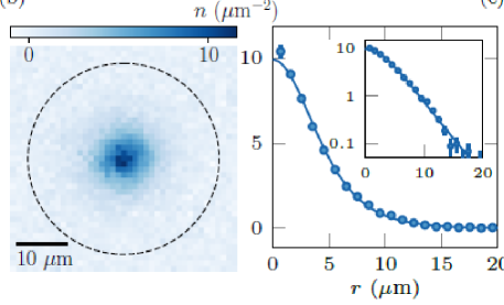
Figure 5: Left: the experimentally observed density distribution in a quasi-stable TS (Townes soliton) created in a minority component of a binary condensate of ⁸⁷Rb atoms, embedded in a majority background. The effective self-attraction in the minority component, which is necessary to build the TS, is induced by the immiscibility of the binary system. Right: the experimentally observed radial profile of the same TS (the chain of dots), fitted to the respective numerical solution of Eq. (3.5). The inset shows the same data on the semilog scale, highlighting the exponentially decaying structure of the TS’s tails (source: Bakkali-Hassani et al., 2021).

IV The central issue: stabilization schemes for multidimensional solitons

IV.1 Scalar (single-component) models in free space (no external potential)

The simplest possibility to arrest the onset of the collapse, and thus stabilize multidimensional fundamental solitons, is to introduce 2D and 3D versions of the NLS equation with the cubic-quintic (CQ) nonlinearity, i.e.,

$$i\psi_{t}+\frac{1}{2}\nabla^{2}\psi+|\psi|^{2}\psi-|\psi|^{4}\psi=0,$$ (71)

where all coefficients may be set equal to $\pm 1$ by means of obvious rescaling. The 2D version of Eq. (4.1) can be implemented in optics, considering the light propagation in a bulk waveguide filled by a dielectric material whose intrinsic optical nonlinearity may be accurately approximated by the combination of the cubic self-focusing and quintic defocusing, such as liquid carbon disulfide (Tominaga and Yoshihara, 1995; Kong et al., 2009; Edilson et al., 2013).

The same CQ nonlinearity in optics can be also realized in colloidal suspensions of metallic nanoparticles (Reyna and de Araújo, 2017). In the latter case, the size and concentration of the particles may be used as parameters controlling actual values of coefficients in front of the cubic and quintic terms in the counterpart of Eq. (4.1), written in the original physical units (before the rescaling is applied to cast the NLS equation in the form Eq. (4.1)). Furthermore, in a particular region of values of the control parameters, the colloid may feature the effective optical nonlinearity including a septimal (seventh-order) term too. In the appropriately scaled form, the cubic-quintic-septimal generalization of Eq. (4.1) takes the form of

$$i\psi_{t}+\frac{1}{2}\nabla^{2}\psi+\sigma_{3}|\psi|^{2}\psi-\sigma_{5}|\psi|^{4}\psi-|\psi|^{6}\psi=0,$$ (72)

where it is assumed that the highest septimal term is self-defocusing (to prevent the onset of the collapse), while the coefficients in front of the cubic and quintic ones, $\sigma_{3}$ and $\sigma_{5}$, may have any sign. In fact, the rescaling makes it possible to set $\sigma_{5}=\pm 1$ (unless $\sigma_{5}=0$), keeping $\sigma_{3}$ as an irreducible parameter which is allowed to take any positive or negative real value. Furthermore, Reyna and de Araújo (2014) had experimentally demonstrated a regime in which the competing nonlinearities are represented by the quintic and septimal terms, while the cubic one nearly vanishes ($\sigma_{3}\approx 0$).

Similar nonlinearities of the CQ type occur in other optical media too, including chalcogenide glasses, with a chemical composition different from usual optical silica (Boudebs et al., 2003), organic materials (stilbazolium derivatives, as shown experimentally by Zhan et al., 2002), and cold atomic gases (Greenberg and Gauthier, 2012). Furthermore, it was demonstrated by Reshef et al. (2017) that the CQ nonlinearity is a generic feature of optical systems with a low linear refractive index (they play an important role in modern photonics, known as “epsilon-near-zero” media, see reviews by Liberal and Engheta (2017), and Niu et al. (2018)). It is also relevant to mention that artificial CQ nonlinearity can be constructed by means of the cascading mechanism, which induces a higher-order effective nonlinearity as a chain of lower-order ones (Dolgaleva, Shin, and Boyd, 2009).

The addition of the defocusing cubic term represents an effect of saturation of the underlying cubic self-focusing. In other cases, the saturation is adequately modeled by the NLS equation with rational, rather than polynomial, nonlinearity:

$$i\psi_{t}+\frac{1}{2}\nabla^{2}\psi+\frac{|\psi|^{2}}{1+|\psi|^{2}}\psi=0.$$ (73)

This equation was introduced by Anderson and Bonnedal (1979) for the propagation of laser beams in plasmas. Essentially the same type of the saturation finds important realizations in optics as a model for the propagation of light beams in semiconductor-doped glasses (Rossignol et al, 1987; Coutaz and Kull, 1991), as well as for beams with extraordinary polarization in photorefractive (PhR) crystals (Segev et al., 1992; Efremidis et al. 2002). Note that, by means of transformation $\psi=\exp\left(it\right)\tilde{\psi}$, Eq. (4.3) can be written in another form, which is often used too:

$$i\tilde{\psi}_{t}+\frac{1}{2}\nabla^{2}\tilde{\psi}-\frac{1}{1+|\tilde{\psi}|^{2}}\tilde{\psi}=0.$$ (74)

A very essential difference of the saturable nonlinearity, as it is written in Eqs. (4.3) or (4.4), from the CQ term in Eq. (4.1) is the fact that the saturable nonlinearity may stabilize only fundamental 2D solitons, while their counterparts with embedded vorticity remain completely unstable against spontaneous splitting (Firth and Skryabin, 1997). On the contrary, the combination of the cubic self-focusing and quintic defocusing can stabilize 2D solitons with any integer value of embedded vorticity (winding number) $S$ (Quiroga-Texeiro and Michinel, 1997; Malomed, Crasovan, and Mihalache, 2002; Davydova and Yakimenko, 2004), although for $S\geq 3$ the stability region becomes very narrow, see Eq. (4.14) below (Pego and Warchall, 2002). Solutions for vortex solitons are looked for by means of the same substitution as written above in Eq. (3.7), which leads to the following radial equation for the stationary wave amplitude:

$$\mu\phi_{S}+\frac{1}{2}\left(\frac{d^{2}\phi_{S}}{dr^{2}}+\frac{1}{r}\frac{d\phi_{S}}{dr}-\frac{S^{2}}{r^{2}}\phi_{S}\right)+\phi_{S}^{3}-\phi_{S}^{5}=0,$$ (75)

cf. Eq. (3.8). The stability of these states is investigated by taking perturbed solutions in the same form (3.29) as introduced above. Then, the linearization leads to the system of equations for small perturbations, of the BdG type, which is a straightforward extension of Eqs. (3.30) and (3.31):

$$\left(i\Gamma+\mu\right)u+\frac{1}{2}\left(\frac{d^{2}u}{dr^{2}}+\frac{1}{r}\frac{du}{dr}-\frac{\left(S+L\right)^{2}}{r^{2}}u\right)$$

$$+\phi_{S}^{2}(r)\left(2u+v\right)-\phi_{S}^{4}\left(3u+2v\right)=0,$$ (4.6)

$$\left(-i\Gamma+\mu\right)v+\frac{1}{2}\left(\frac{d^{2}v}{dr^{2}}+\frac{1}{r}\frac{dv}{dr}-\frac{\left(S-L\right)^{2}}{r^{2}}v\right)$$

$$+\phi_{S}^{2}(r)\left(2v+u\right)-\phi_{S}^{4}\left(2u+3v\right)=0.$$ (4.7)

Equations (4.6) and (4.7) should be supplemented, as above, by b.c. (3.32).

The NLS equation with the saturable quintic self-focusing (without cubic terms),

$$i\psi_{t}+\frac{1}{2}\nabla^{2}\psi+\frac{|\psi|^{4}}{1+|\psi|^{4}}\psi=0,$$ (76)

cf. Eq. (4.3), may be a relevant model as well, applying, in a certain parameter region, to the light propagation in a waveguide filled with liquid carbon disulfide (Reyna et al., 2016).

In all these realizations of the NLS equation with the polynomial (in particular, CQ) or saturable nonlinearity in optics, $t$ is actually the propagation distance (usually denoted $z$, in that context), and the relevant realization is two-dimensional, with transverse coordinates $\left(x,y\right)$ in the bulk waveguides modeled by these equations. The full 3D realization would make it necessary to consider the spatiotemporal propagation in the same waveguides, which is far from implementation in experiments.

IV.2 The wave field in the trapping potential

Another generic possibility to stabilize 2D and 3D solitons against the collapse driven by the cubic self-focusing, and to partly stabilize vortex solitons against the splitting instability, is to add a trapping potential to the multidimensional NLS/GP equation. The usually considered potential is a straightforward multidimensional extension of the one-dimensional HO potential (2.2). Thus, in the 3D case, Eq. (3.1) is replaced by

$$i\psi_{t}+\frac{1}{2}\nabla^{2}\psi+|\psi|^{2}\psi-\frac{1}{2}\left[\Omega_{x,y}^{2}\left(x^{2}+y^{2}\right)+\Omega_{z}^{2}z^{2}\right]\psi=0.$$ (77)

This form of the HO potential implies a possibility of its anisotropy, with $\Omega_{z}^{2}\neq$ $\Omega_{x,y}^{2}$, which keeps the axial symmetry in the $\left(x,y\right)$ plane (this is the usual situation which takes place in experiments (Pitaevskii and Stringari, 2003)), but breaks the spherical symmetry. In principle, one may also consider a fully anisotropic potential, with $\Omega_{x}^{2}\neq\Omega_{y}^{2}$. In optics, the NLS equation may be three-dimensional, modeling the spatiotemporal propagation of light in the bulk waveguide, but the trapping potential may only be two-dimensional, which corresponds to $\Omega_{z}=0$ in Eq. (4.10), as the potential cannot be a quadratic function of time.

Stationary solutions of Eq. (4.10), with vorticity $S$, are naturally looked for, in cylindrical coordinates,

$$\left\{\rho\equiv\sqrt{x^{2}+y^{2}},\theta,z\right\}$$ (78)

as a 3D version of ansatz (3.7):

$$\psi=e^{-i\mu t+iS\theta}\phi_{S}\left(\rho,z\right),$$ (79)

with real function $\phi_{S}$ satisfying equation

$$\mu\phi_{S}+\frac{1}{2}\left(\frac{d^{2}\phi_{S}}{d\rho^{2}}+\frac{1}{\rho}\frac{d\phi_{S}}{d\rho}-\frac{S^{2}}{\rho^{2}}\phi_{S}+\frac{d^{2}\phi_{S}}{dz^{2}}\right)+\phi_{S}^{3}$$

$$-\frac{1}{2}\left(\Omega_{x,y}^{2}\rho^{2}+\Omega_{z}^{2}z^{2}\right)\phi_{S}=0.$$ (4.12)

The NLS/GP equation (4.9) with the axially symmetric but spherically asymmetric trapping potential conserves three dynamical invariants, viz., the norm (see also Eq. (3.22))

$$N=\int\int\int dxdydz\left|\psi\left(x,y,z,t\right)\right|^{2},$$ (80)

$z$-component of the angular momentum,

$$M_{z}=-i\int\int\int dxdydz\psi^{\ast}\left(x\frac{\partial\psi}{\partial y}-y\frac{\partial\psi}{\partial x}\right)\equiv-i\int_{0}^{\infty}\rho d\rho\int_{0}^{2\pi}d\theta\int_{-\infty}^{+\infty}dz\psi^{\ast}\frac{\partial\psi}{\partial\theta}$$ (81)

(it is written here in terms of both the Cartesian coordinates and cylindrical ones, defined as per Eq. (4.10)), and the Hamiltonian (cf. Eq. (3.3)):

$$H=\frac{1}{2}\int\int\int dxdydz\left\{\left|\nabla\psi\right|^{2}-|\psi|^{4}+\left[\Omega_{x,y}^{2}\left(x^{2}+y^{2}\right)+\Omega_{z}^{2}z^{2}\right]|\psi|^{2}\right\}.$$ (82)

In the case when the HO potential is isotropic, with $\Omega_{x,y}^{2}=\Omega_{z}^{2}$, Eq. (4.9) conserves not only the $z$-component (4.14), but the full vectorial angular momentum,

$$\mathbf{M}=-i\int\int\int dxdydz\psi^{\ast}\left(\mathbf{r}\times\nabla\right)\psi.$$ (83)

In the general form, the stability of the stationary states is addressed by looking for a perturbed solution of Eq. (4.10), in the cylindrical coordinates, as

$$\psi\left(r,\theta,z,t\right)=e^{-i\mu t+iS\theta}\left\{\phi_{S}(\rho,z)+\varepsilon\left[e^{iL\theta+\Gamma t}u(\rho,z)+e^{-iL\theta+i\Gamma^{\ast}t}v^{\ast}(\rho,z)\right]\right\},$$ (84)

which is a straightforward extension of the 2D ansatz (3.29). The substitution of this in Eq. (4.9) and linearization with respect to the small amplitude $\varepsilon$ of the perturbation leads to the corresponding system of the BdG equations,

$$\left(i\Gamma+\mu\right)u+\frac{1}{2}\left[\frac{d^{2}u}{d\rho^{2}}+\frac{1}{\rho}\frac{du}{d\rho}-\frac{\left(S+L\right)^{2}}{\rho^{2}}u+\frac{d^{2}u}{dz^{2}}\right]$$

$$+\phi_{S}^{2}(\rho,z)\left(2u+v\right)-\frac{1}{2}\left(\Omega_{x,y}^{2}\rho^{2}+\Omega_{z}^{2}z^{2}\right)u=0,$$ (4.18)

$$\left(-i\Gamma+\mu\right)v+\frac{1}{2}\left[\frac{d^{2}v}{dr^{2}}+\frac{1}{r}\frac{dv}{dr}-\frac{\left(S-L\right)^{2}}{r^{2}}v+\frac{d^{2}v}{dz^{2}}\right]$$

$$+\phi_{S}^{2}(\rho,z)\left(2v+u\right)-\frac{1}{2}\left(\Omega_{x,y}^{2}\rho^{2}+\Omega_{z}^{2}z^{2}\right)v=0,$$ (4.19)

cf. Eqs. (3.30), (3.31) and (4.6), (4.7). Equations (4.18) and (4.19) should be solved numerically, subject to b.c.

$$u\sim\rho^{\left|S+L\right|},v\sim\rho^{\left|S-L\right|}~{}\mathrm{at}~{}\rho\rightarrow 0,$$ (85)

cf. Eq. (3.32).

IV.3 Spatially periodic potentials

Optical-lattice (OL) potentials, which may be induced, as interference patterns, by pairs of counter-propagating laser beams illuminating the BEC, provide a versatile toolbox for experimental and theoretical studies of atomic condensates (Brazhnyi and Konotop, 2004; Morsch and Oberthaler, 2006; Lewenstein, Sanpera, and Ahufinger, 2012; Dutta et al., 2015). The general 3D form of the OL potential is

$$U\left(x,y,z\right)=-\left[\left(V_{0}\right)_{x}\cos\left(\frac{2\pi}{L_{x}}x\right)+\left(V_{0}\right)_{y}\cos\left(\frac{2\pi}{L_{y}}y\right)+\left(V_{0}\right)_{z}\cos\left(\frac{2\pi}{L_{z}}z\right)\right],$$ (86)

where different amplitudes $\left(V_{0}\right)_{x,y,z}$ and periods $L_{x,y,z}$ imply a possibility to consider anisotropic lattice potentials, and the respective NLS/GP equation is written as

$$i\psi_{t}+\frac{1}{2}\nabla^{2}\psi+|\psi|^{2}\psi+U\left(x,y,z\right)\psi=0.$$ (87)

The 3D lattice potential is sufficient to stabilize both fundamental and vortex solitons. In particular, although the periodic potential breaks the spatial isotropy, the soliton’s vorticity (alias the winding number) may be unambiguously defined in this case too (Baizakov, Malomed, and Salerno, 2003; Yang and Musslimani, 2003).

The 2D reduction of the three-dimensional OL potential (4.21) is obvious. An essential finding is that the quasi-2D lattice potential in the 3D space, i.e., potential (4.21) with $\left(V_{0}\right)_{z}=0$, is sufficient for the stabilization of fully three-dimensional solitons; similarly, the quasi-1D potential, with only $\left(V_{0}\right)_{x}\neq 0$, is sufficient for the stabilization of 2D solitons, although the quasi-1D lattice cannot stabilize full 3D solitons (Baizakov, Malomed, and Salerno, 2004; Mihalache et al., 2004a; Leblond, Malomed, and Mihalache, 2007).

Another relevant form of the OL potential in the 2D space (as well as a quasi-2D potential in 3D) is a radial lattice. The corresponding 2D NLS/GP equation takes the form of

$$i\psi_{t}+\frac{1}{2}\nabla^{2}\psi+|\psi|^{2}\psi-V\left(\rho\equiv\sqrt{x^{2}+y^{2}}\right)\psi=0,$$ (88)

where the radial potential was considered in various forms – in particular, as

$$V_{\mathrm{Bessel}}(\rho)=-V_{0}J_{0}(\rho/a),$$ (89)

with Bessel function $J_{0}(\rho/a)$, by Kartashov, Vysloukh, and Torner (2004), and as the radially periodic potential,

$$V_{\cos}(\rho)=-V_{0}\cos\left(2k\rho\right),$$ (90)

(cf. Eq. (2.62)) by Baizakov, Malomed, and Salerno (2006).

In optics, the underlying NLS equation may be three- or two-dimensional, for the spatiotemporal or spatial-domain propagation, respectively, The effective periodic potential, representing the photonic-crystal structure in this equation (including its 3D version) may be solely two-dimensional, corresponding to the spatially-periodic modulation of the local refractive index in the transverse plane (see books by Joannopoulos et al. (2008), Skorobogatiy and Yang (2009), and Yang (2010)).

A powerful method, which has made it possible to create many species of 2D optical solitons in PhR materials (see the review by Lederer et al. 2008), was proposed and implemented by Efremidis et al. (2002, 2003). It makes use of the fact that the light with ordinary polarization propagates linearly in PhR crystals, hence interference of laser beams with such polarization can be used to induce an effective (virtual) lattice pattern in the bulk material, while light with the extraordinary polarization, illuminating the same material, is subject to the action of strong saturable nonlinearity (Segev et al., 1992). The result includes self-focusing of the extraordinarily-polarized probe beam (as in Eq. (4.4)) and the XPM-mediated action of the virtual lattice potential, which is optically induced by the interference pattern in the ordinary polarization. The effective 2D equation for the spatial-domain propagation of the probe field $u$ is (Efremidis et al. (2002, 2003))

$$iu_{z}+\frac{1}{2}\left(u_{xx}+u_{zz}\right)-\frac{E_{0}u}{1+|u|^{2}+U_{0}\left[\cos\left(2\pi x/L_{x}\right)+\cos\left(2\pi y/L_{y}\right)\right]},$$ (91)

where $z$ is the propagation constant, $\left(x,y\right)$ are the transverse coordinates, $U_{0}$ is the strength of the virtual lattice potential, and $E_{0}$ is the dc electric field which induces the saturable nonlinearity (self-focusing and defocusing for $E_{0}>0$ and $E_{0}<0$, respectively). Thus, Eq. (4.26) introduces a 2D model similar to one based on Eqs. (4.22) and (4.21), but with a more complex structure. Note that the lowest-order expansion of Eq. (4.26) for small $|u|^{2}$ and $U_{0}$ reduces to the 2D version of Eq. (4.22).

The above models with lattice potentials, based on Eqs. (4.22) and (4.23), are written with the self-focusing (self-attractive) sign in front of the cubic term. In realization provided by optical media, this is virtually always the case. In BEC, the opposite, self-repulsive nonlinearity, is more typical, corresponding to natural repulsive interactions between atoms in the BEC, although the sign may be switched to the attraction by means of FR. In the case of the self-repulsive nonlinearity, 2D and 3D self-trapped states can be created, with the help of the OL potential, as gap solitons. Further, stable 2D gap solitons with intrinsic vorticity were constructed by Sakaguchi and Malomed (2004), see examples in Fig. 6.

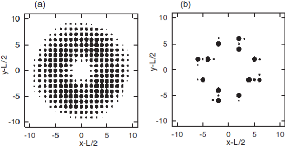
Figure 6: Typical examples of stable 2D gap solitons with embedded vorticity $S=2$, produced by the two-dimensional NLS/GP equation with a lattice potential (the 2D version of potential (4.21)) and self-repulsive cubic nonlinearity. Panels (a) and (b) display density distributions in loosely- and tightly bound vortex gap solitons, respectively (source: Sakaguchi and Malomed, 2004b).

IV.4 Nonlinear trapping potentials

Potentials based on attractive nonlinearities

Quite interesting predictions for the creation of stable multidimensional soliton-like (self-trapped) states were reported using the NLS/GP equation with effective nonlinear potentials induced by local modulation of the coefficient in front of the cubic term in the equation. The general form of the equation is

$$i\psi_{t}+\frac{1}{2}\nabla^{2}\psi+g(x,y,z)|\psi|^{2}\psi=0.$$ (92)

Following the terminology used since long ago in solid-state physics (Harrison, 1966), such settings are sometimes referred to as pseudopotentials. In optics, 1D and 2D versions of this model can be realized in media with spatially inhomogeneous distributions of density of resonant dopants, which affect the local strength of the self-focusing (Hukride, Runde, and Kip, 2003). In BEC, Eq. (4.27) can be implemented in the space of any dimension by means of FR with the local strength controlled by a spatially inhomogeneous dc magnetic field (Ghanbari et al., 2006; Bauer et al., 2009) or by an appropriately patterned optical field, which also can also control the FR (Yamazaki et al., 2010; Clark et al., 2015).

Many theoretical and experimental results obtained for solitons supported by spatially periodic nonlinear potentials, as well as by combinations of nonlinear and linear lattices, were summarized in a review by Kartashov, Malomed, and Torner (2011). A majority of these results pertain to 1D setups. 2D nonlinear lattices can support stability of solitons against the collapse under special conditions, such as a necessity to use nonlinear potentials with sharp edges. Examples of 2D settings of the latter type were elaborated, in particular, for the 2D version of Eq. (4.27) with radial modulation profiles in the form of an annulus (Sakaguchi and Malomed, 2006) or step-wise structure (Sakaguchi and Malomed, 2012), i.e.,

$$i\psi_{t}+\frac{1}{2}\nabla^{2}\psi+g(r)|\psi|^{2}\psi=0,$$ (93)

with, respectively,

$$g_{\mathrm{annulus}}(r)=\begin{array}[]{c}1,~{}\mathrm{at~{}}r_{\min}<r<r_{\max},\\ 0,~{}\mathrm{at~{}}r<r_{\min}~{}\mathrm{and}~{}r>r_{\max},\end{array}$$ (94)

or

$$g_{\mathrm{step}}(r)=\begin{array}[]{c}1,~{}\mathrm{at~{}}r<r_{\max},\\ 1-\Delta g,~{}\mathrm{at~{}}r>r_{\max},\end{array}$$ (95)

where constraint $0<\Delta g<1$ is imposed. The modulation profile (4.29) maintains stable 2D solitons, provided that the annulus is not too narrow, viz., for $r_{\min}/r_{\max}<0.47$, while profile (4.30) provides stability of 2D solitons in an interval $\Delta N$ of the norm around its TS value (3.12) which scales $\sim\Delta g$ for $\Delta g\ll 1$.

Potentials based on the repulsive nonlinearity

A different option for the creation of highly stable self-trapped states was proposed by Borovkova et al. (2011a,b). It is based on Eq. (4.28) with the self-defocusing (repulsive) nonlinearity, $g(r)<0$, whose local strength, $\left|g(r)\right|$, diverges at $r\rightarrow\infty$ as

$$g(r\rightarrow\infty)\approx-g_{0}r^{\alpha},$$ (96)

with positive constant $g_{0}$ (Borovkova et al. 2011a), or faster – in particular, as an anti-Gaussian, i.e.,

$$g(r\rightarrow\infty)\approx-g_{0}\exp\left(r^{2}/r_{0}^{2}\right)$$ (97)

(Borovkova et al. 2011b). The corresponding stationary 3D and 2D solutions with chemical potential $\mu>0$ are looked for as

$$\psi_{\mathrm{3D}}=e^{-i\mu t}\phi(r),\psi_{\mathrm{2D}}=e^{-i\mu t+iS\theta}\phi(r),$$ (98)

where $S=0,1,2,...$ is vorticity, $S=0$ corresponding to the ground state (fundamental stationary solution). The substitution of ansatz (4.33), with dimension $D=3$ or $2$, in Eq. (4.28) leads to the respective stationary equation,

$$\mu\phi+\frac{1}{2}\left(\frac{d^{2}\phi}{dr^{2}}+\frac{D-1}{r}\frac{d\phi}{dr}-\frac{S^{2}}{r^{2}}\phi\right)+g(r)\phi^{3}$$ (99)

(term $S^{2}/r^{2}$ appears here only in the 2D case).

Although the nonlinearity in Eq. (4.28) is self-repulsive at all values of $r$, the fact that the repulsion is stronger at large $r$ suggest a possibility to produce self-trapped states. This possibility is clearly confirmed by the TF approximation, which neglects derivatives in Eq. (4.34) and thus yields the following approximate solution of this equation:

$$\phi_{\mathrm{TF}}^{2}(r)=\left\{\begin{array}[]{c}\left(\mu-S^{2}r^{-2}\right)/\left|g(r)\right|,~{}\mathrm{at}~{}r>S/\sqrt{\mu},\\ 0,~{}\mathrm{at}~{}r<S/\sqrt{\mu}\end{array}\right.$$ (100)

(obviously, this approximation makes sense only for $\mu>0$). The “inner hole” in the 2D version of this expression at $r<S/\sqrt{\mu}$ (with $S\geq 1$) is a known artifact of the TF approximation (see a review by Fetter (2009)), while the actual solution has the usual asymptotic form at $r\rightarrow 0$, namely, $\phi(r)\approx\mathrm{const}\cdot r^{|S|}$. The applicability condition for the TF approximation is

$$\left(dg/dr\right)^{2}\ll\mu g^{2},$$ (101)

which, in particular, always holds at large $r$ for $g(r)$ given by Eq. (4.31).

A necessary condition for the self-trapping is the convergence of the total norm corresponding to the TF approximation,

$$N_{\mathrm{TF}}=2\pi(D-1)\int_{0}^{\infty}\phi_{\mathrm{TF}}^{2}(r)r^{D-1}dr.$$ (102)

Thus, for $g(r)$ with the power-law asymptotic form (4.31), the integral in Eq. (4.37) converges for $\alpha>D$, as well as for $g(r)$ with the anti-Gaussian asymptotic form (4.32).

For $g(r)$ with $\alpha<D$ in Eq. (4.31), it was demonstrated by Zeng and Malomed (2017) that 2D solutions of Eq. (4.34), as well as their 1D counterparts (they are produced by Eq. (4.34) with $D=1$, $S=0$, and $r$ replaced by $x$, while $r$ is replaced by $|x|$ in Eq. (4.31)), are meaningful too. They include localized continuous waves (CWs), globally approximated by the TF expression (4.35) with $S=0$, as well as localized dark vortices in 2D, and localized dark solitons in 1D (including bound states of dark solitons). These are modes of such types created on top of the weakly localized CWs. They feature nontrivial stability boundaries in the respective parameter spaces (in particular, bound states of localized dark solitons are weakly unstable, while localized dark vortices with $S=2$ may be stable).

IV.5 The Gross-Pitaevskii (GP) equation with Lee-Huang-Yang (LHY) corrections for quantum droplets (QDs)

The 3D model

The recent progress in both theoretical and experimental work with multidimensional soliton-like (self-trapped) objects has been greatly advanced by the advent of the concept of QDs, proposed by Petrov (2015). It offers a practically feasible possibility to suppress the collapse in 3D and 2D binary (two-component) BEC with attractive interactions, thus making it possible to create stable self-trapped “droplets”, which are usually not called solitons, but are quite similar states. Actually, the term “droplet” is adopted because the condensate density in them cannot exceed a certain maximum value, making this quantum state of matter effectively incompressible, similar to fluids.

In terms of the theory, the analysis of Petrov (2015) led to the 3D GP equation with an extra quartic term suppressing the onset of the collapse driven by the usual cubic self-attraction. The extra term is induced by the Lee-Hung-Yang effect (Lee, Huang, and Yang, 1957), which represents an effective correction induced by quantum fluctuations around the MF (mean-filed) states described by the GP equation.

To derive the LHY correction, one starts with the energy density of the binary BEC in the MF approximation:

$$\mathcal{E}_{\mathrm{MF}}=\frac{1}{2}g_{11}n_{1}^{2}+\frac{1}{2}g_{22}n_{2}^{2}+g_{12}n_{1}n_{2},$$ (103)

where $g_{11,22}>0$, and $g_{12}<0$ are coupling constants which determine, respectively, the strengths of the self-repulsive interaction between atoms in the same species (component), and cross-attraction between atoms belonging to different species, while $n_{1,2}$ are atomic densities of the two species. The combination of the intra-component repulsion and cross-component attraction makes the binary condensate obviously miscible. In the MF approximation, the collapse occurs if the cross-attraction is effectively stronger than the self-repulsion, which means

$$-g_{12}>\sqrt{g_{11}g_{22}}.$$ (104)

In the experiments of Cabrera et al. (2018), Cheiney et al. (2018), and Semeghini et al. (2018), the two species were realized as atomic states of ³⁹K, viz., $\left|F,m_{F}\right\rangle=\left|1,-1\right\rangle$ and $\left|1,0\right\rangle$, where $F$ and $m_{F}$ stand, respectively, for the total angular momentum of the potassium atom and its $z$-component. In this case, scattering lengths $a_{s}$ of repulsive collisions are the same for both species, suggesting to define

$$g_{11}=g_{22}\equiv g=4\pi\hbar^{2}m/a_{s},$$ (105)

while the inter-species attraction is controlled by means of FR.

The LHY correction to the energy density (4.38) was derived by Petrov (2015) as a contribution from the zero-point energy of the Bogoliubov excitations around the MF state with equal densities of the mixed components, $n_{1}=n_{2}\equiv n$:

$$\mathcal{E}_{\mathrm{LHY}}=\frac{128}{30\sqrt{\pi}}gn^{2}\sqrt{na_{s}^{3}},$$ (106)

where $m$ is the atomic mass. In a dilute condensate, the LHY term (4.41), $\sim n^{5/2}$ is, generally, much smaller than the MF ones, $\sim n^{2}$ , in Eq. (4.38), hence the LHY correction is negligible, as one might expect. However, when FR is used to tune $g_{12}$ so that it is close to the equilibrium point, $g_{12}=-g$ (see Eq. (4.39)), at which the MF self-repulsion is nearly balanced by a slightly stronger cross-attraction between the components, the LHY term becomes essential. Thus, one can define the parameter of the weak residual MF attraction,

$$0<-\delta g\equiv-\left(g_{12}+g\right)\ll g.$$ (107)

The final result is the LHY-corrected GP equation in 3D for equal wave functions $\psi$ of both components, derived by Petrov (2015) in the following scaled form:

$$i\psi_{t}+\frac{1}{2}\nabla^{2}\psi+3|\psi|^{2}\psi-\frac{5}{2}|\psi|^{3}\psi,$$ (108)

cf. the usual GP equation (4.27). Here, the quartic self-repulsive term, $\left(5/2\right)|\psi|^{3}\psi$, represents the LHY correction which prevents the onset of the collapse.

The derivation of the LHY-amended GP was revised by Hu and Liu (2020), who have taken into regard the pairing field. Finite-temperature effects, which can essentially change the structure and stability of QDs were considered in detail by Wang, Liu, and Hu (2021).

It is relevant to mention that, in addition to theoretically predicted (Petrov, 2015) and experimentally demonstrated (Cabrera et al., 2018, Cheiney et al., 2018, and Semeghini et al., 2018) fundamental QD states, their stable counterparts with embedded vorticity $S=1$ and $2$ were predicted too (Kartashov et al., 2018).

Lower dimensions: 2D and 1D

Under the action of extremely tight confinement applied in direction ($z$), reduction of the 3D equation (4.43) to a 2D model was carried out by Petrov and Astrakharchik (2016). In this case, the energy density of the binary BEC with equal densities $n$ of the two components becomes

$$\mathcal{E}_{\mathrm{2D}}=\frac{8\pi n^{2}}{\ln^{2}(\left|a_{12}\right|/a_{s})}\left[\ln\left(\frac{n}{\left(n_{0}\right)_{\mathrm{2D}}}\right)-1\right],$$ (109)

where $a_{s}>0$ is the same as in Eq. (4.40), $a_{12}<0$ is the scattering length corresponding of the the attractive inter-species interaction, and the reference density is

$$\left(n_{0}\right)_{\mathrm{2D}}=\left(2\pi\right)^{-1}\exp\left(-2\gamma-3/2\right)\left(a_{s}\left|a_{12}\right|\right)^{-1}\ln(\left|a_{12}\right|/a_{s})$$ (110)

($\gamma\approx 0.5772$ is the Euler’s constant), cf. Eqs. (4.38) and (4.41) in the 3D situation. The corresponding 2D LHY-amended GPE for equal wave functions of both components is

$$i\partial_{t}\psi=-\frac{1}{2}\nabla^{2}\psi+\frac{8\pi}{\text{ln}^{{\large 2}}(\left|a_{{\large 12}}\right|/a_{{\large s}})}\ln\left(\frac{|\psi|^{{\Large 2}}}{\sqrt{e}\left(n_{{\Large 0}}\right)_{\mathrm{2D}}}\right)|\psi|^{2}\psi.$$ (111)

For the theoretical analysis, it is convenient to cast this equation in the following scaled form:

$$i\partial_{t}\psi=-\frac{1}{2}\nabla^{2}\psi+\ln\left(|\psi|^{2}\right)|\psi|^{2}\psi.$$ (112)

The increase of density from $|\psi|^{2}<1$ to $|\psi|^{2}>1$ leads to the change of the sign of the logarithmic factor in Eq. (4.45). As a result, the cubic term in this equation is self-focusing at $|\psi|^{2}<1$, maintaining the formation of QDs, and defocusing at $|\psi|^{2}>1$, thus arresting the transition to the collapse, and securing the stability of 2D QDs. Furthermore, Eq. (4.45) gives rise to stable QDs with embedded vorticity $S$ – at least, up to $S=5$ (Li et al., 2018).

For the 1D setting with extremely tight confinement in the two transverse directions, the analysis performed by Petrov and Astrakharchik (2016) yields the following effective energy density:

$$\mathcal{E}_{\mathrm{1D}}=\delta g\cdot n^{2}-\frac{4\sqrt{2}}{3\pi}(gn)^{3/2},$$ (113)

cf. Eqs. (4.38), (4.41), and (4.44), where $\delta g$ and $g$ are the same coefficients as in Eqs. (4.40) and (4.42) The respective LHY-amended GP equation features a combination of the usual MF cubic nonlinearity and a quadratic term, representing the LHY correction in the 1D setting:

$$i\partial_{t}\psi=-(1/2)\partial_{xx}\psi+\delta g\cdot|\psi|^{2}\psi-(\sqrt{2}/\pi)g^{3/2}|\psi|\psi.$$ (114)

Note that the LHY-induced quadratic term is self-focusing in Eq. (4.47), on the contrary to the defocusing sign of the quartic term in the 3D equation (4.43). Because the most interesting results for QDs are obtained in the case of the competition between the residual MF term and the LHY-induced correction, in the 1D case the relevant situation is one with $\delta g>0$, when the residual MF self-interaction is repulsive, in contrast with the residual self-attraction adopted in the 3D setting, as mentioned above.

The effectively 2D and 1D description outlined above is valid for extremely strong transverse confinement, with the characteristic size $l_{\mathrm{confinement}}\ll l_{\mathrm{healing}}\sim 30$ nm, where $l_{\mathrm{healing}}$ is the healing length in the BEC for experimentally relevant settings, such as those realized in the experimental works by Cabrera et al. (2018), Cheiney et al. (2018), and Semeghini et al (2018). In reality, the values of $l_{\mathrm{confinement}}$ in the experiment is $\gtrsim 0.5$ $\mathrm{\mu}$m. For this reason, the dimension crossover $\mathrm{3D\rightarrow 2D}$ requires a more careful consideration. In particular, for a relatively loosely confined (“thick”) quasi-2D layer of BEC it may be relevant to consider the 2D version of Eq. (4.43), keeping the quartic LHY term (Shamriz, Chen, and Malomed, 2020a). Detailed consideration of the dimension reductions, $\mathrm{3D\rightarrow 2D}$ and $\mathrm{3D\rightarrow 1D}$, beyond the first approximation presented by Petrov and Astrakharchik, was elaborated by Zin et al. (2018), Ilg et al. (2018), and Lavoine and Bourdel (2021).

IV.6 Spinor (two-component) BEC models

IV.6.1 Spin-orbit-coupled BEC in two dimensions

Ultracold atomic gases in the BEC state are often used as testbeds for emulating, in a simple clean form, various effects known in complex settings of condensed matter physics (Lewenstein, Sanpera, and Ahufinger, 2012; Hauke et al., 2012). One of important effects emulated by binary BECs is the spin-orbit coupling (SOC), originally discovered in semiconductors, as the weakly-relativistic interaction of the spin of moving electrons with the electrostatic field of the ionic lattice (Dresselhaus, 1955; Bychkov and Rashba, 1984). Although the true spin of bosonic atoms, used for this purpose, is zero, the spinor wave function of electrons may be mapped into the two-component wave function of the condensate, thus realizing pseudospin $1/2$ (Lin, Jiménez-García, and Spielman, 2011; Galitski and Spielman, 2013). While most experimental work on this topic addressed effectively 1D settings, the realization of the SOC in the 2D binary BEC was reported too, by Wu et al. (2016). The 2D and 3D realizations are obviously necessary for the creation of multidimensional solitons.

In the MF approximation, the system of effectively two-dimensional GP equations for the two-component wave function, $\left(\psi_{+},\psi_{-}\right)$, can be written as follows (Zhang, Mao, and Zhang, 2012; Sakaguchi et al., 2018):

$$i\frac{\partial\psi_{+}}{\partial t}=-\frac{1}{2}\nabla^{2}\psi_{+}+\left(\lambda_{R}\widehat{D}^{[-]}\psi_{-}-i\lambda_{D}\widehat{D}^{[+]}\psi_{-}\right)-(|\psi_{+}|^{2}+\gamma|\psi_{-}|^{2})\psi_{+}-\Omega\psi_{+},$$ (115)

$$i\frac{\partial\psi_{-}}{\partial t}=-\frac{1}{2}\nabla^{2}\psi_{-}-\left(\lambda\widehat{{}_{R}D}^{[+]}\psi_{+}+i\lambda_{D}\widehat{D}^{[-]}\psi_{+}\right)-(|\psi_{-}|^{2}+\gamma|\psi_{+}|^{2})\psi_{-}+\Omega\psi_{-},$$ (116)

where linear operators

$$\widehat{D}^{[\pm]}\equiv\partial/\partial x\pm i\partial/\partial y$$ (117)

represent SOC of the Rashba and Dresselhaus types, with real strengths $\lambda_{R}$ and $\lambda_{D}$, respectively. Thus, the SOC terms linearly couple two components of the pseudospinor wave function, in Eqs. (4.48) and (4.49), by means of the first spatial derivatives.

The last terms in these equations, with real $\Omega$, represent the Zeeman splitting between the components (if it is present), and the signs in front of the cubic terms, including the cross-nonlinear ones, with $\gamma>0$, correspond to attractive interactions between atoms in the condensate. In this case, the system of Eqs. (4.48) and (4.49) gives rise to 2D solitons which may be stable states realizing the system’s ground state in the 2D setting with cubic attraction (Sakaguchi, Li, and Malomed, 2014). Prior to the publication of the latter result, it was commonly believed that NLS equations with cubic self-attraction can never create stable solitons in 2D settings.

A relevant characteristic of the SOC system (4.48)-(4.50) is the linear dispersion relation for its plane-wave solutions with 2D wave vector $\mathbf{k=}\left(k_{x},k_{y}\right)$,

$$\psi_{\pm}\sim\exp\left(i\mathbf{k}\cdot\mathbf{r}-i\omega t\right).$$ (118)

The substitution of ansatz (4.51) in the linearized version of Eqs. (4.48) and (4.49) yields two branches of the dispersion relation:

$$\omega=\frac{1}{2}k^{2}\pm\sqrt{(\lambda_{R}^{2}+\lambda_{D}^{2})k^{2}+4\lambda_{R}\lambda_{D}k_{x}k_{y}+\Omega^{2}},$$ (119)

which is anisotropic in the plane of $\left(k_{x},k_{y}\right)$. In the special case of

$$\lambda_{D}=\pm\lambda_{R}\equiv\lambda,$$ (120)

which was actually realized by Lin, Jiménez-Garcia and Spielman (2011) in the first experimental demonstration of the SOC in binary BEC, the pseudospin-dependent (second) term in right-hand side of Eq. (4.52) becomes effectively one-dimensional, as it contains a single wave-vector component, either $\left(k_{x}+k_{y}\right)$ or $\left(k_{x}-k_{y}\right)$:

$$\omega=\frac{1}{2}k^{2}\pm\sqrt{2\lambda^{2}(k_{x}\pm k_{y})^{2}+\Omega^{2}}.$$ (121)

The 2D model with a quasi-1D form of SOC, which is actually tantamount to the system of Eqs. (4.48) and (4.49), was recently considered by Kartashov et al. (2020). The respective system is written as

$$\left[i\partial_{t}+\frac{1}{2}\nabla^{2}+i\lambda\sigma_{x}\partial_{x}+\left(\begin{array}[]{cc}\left|\psi_{+}\right|^{2}+\gamma|\psi_{-}|^{2}&0\\ 0&\left|\psi_{-}\right|^{2}+\gamma|\psi_{+}|^{2}\end{array}\right)+\Omega\sigma_{z}\right]\Psi,$$ (122)

where the pseudospinor weave functions is define as $\Phi=\left\{\psi_{+},\psi_{-}\right\}$, $\sigma_{x}$ and $\sigma_{z}$ being the usual Pauli matrices.

The branch of dispersion relation (4.52) with the bottom sign in front of the pseudospin-dependent term splits the axis of $\omega$ into a semi-infinite band, $\omega>\omega_{\min}$, where the branch takes it values, and a semi-infinite spectral gap, $\omega<\omega_{\min}$, where the plane-wave solutions (4.51) of the linearized system of Eqs. (4.48) and (4.49) do not exist. In particular, in the case of $\lambda_{D}=0$ and $\lambda_{R}\equiv\lambda$, or vice versa, the boundary of the semi-infinite gap is

$$\omega_{\min}=\left\{\begin{array}[]{c}-(1/2)\left(\lambda^{2}+\Omega^{2}/\lambda^{2}\right),~{}\mathrm{if}~{}|\Omega|<\lambda^{2},\\ -|\Omega|,~{}\mathrm{if}~{}|\Omega|>\lambda^{2}.\end{array}\right.$$ (123)

The full nonlinear system of Eqs. (4.48) and (4.49) conserves the total norm,

$$N=\iint(|\psi_{+}|^{2}+|\psi_{-}|^{2})dxdy\equiv N_{+}+N_{-},$$ (124)

which is proportional to the number of atoms in the condensate, the vectorial momentum (which is conserved in spite of the absence of the Galilean invariance),

$$\mathbf{P}=i\iint(\psi_{+}^{\ast}\nabla\psi_{+}+\psi_{-}^{\ast}\nabla\psi_{-})dxdy,$$ (125)

cf. Eq. (2.18), and the energy,

$$E=E_{\mathrm{kin}}+E_{\mathrm{int}}+E_{\mathrm{pseudospin}}+E_{\mathrm{Zeeman}},$$ (126)

which includes kinetic, interaction, pseudospin, and Zeeman terms:

$$E_{\mathrm{kin}}=\frac{1}{2}\iint\left(|\nabla\psi_{+}|^{2}+|\nabla\psi_{-}|^{2}\right)dxdy,$$ (127)

$$E_{\mathrm{int}}=-\frac{1}{2}\iint\left[\left(|\psi_{+}|^{4}+|\psi_{-}|^{4}\right)+2\gamma|\psi_{+}|^{2}|\psi_{-}|^{2}\right]dxdy,$$ (128)

$$E_{\mathrm{pseudospin}}=\iint\left[\psi_{+}^{\ast}\left(\lambda_{R}\widehat{D}^{[-]}-i\lambda_{D}\widehat{D}^{[+]}\right)\psi_{-}-\psi_{-}^{\ast}\left(\lambda_{R}\widehat{D}^{[+]}+i\lambda_{D}\widehat{D}^{[-]}\right)\psi_{+}\right]dxdy,$$ (129)

$$E_{\mathrm{Zeeman}}=-\Omega\iint\left(|\psi_{+}|^{2}-|\psi_{-}|^{2}\right)dxdy.$$ (130)

The comparison of Eqs. (4.48) and (4.49) with the underlying system of the GP equations, written in physical units, shows that the unit length in Eqs. (4.48) and (4.49) typically corresponds to the spatial scale $\sim 1$ $\mathrm{\mu}$m. Further, assuming typical values of the transverse confinement length (in the third direction) $\simeq 3$ $\mathrm{\mu}$m and the scattering length of the interatomic attraction $\sim-0.1$ nm, one concludes that $N=1$ in the scaled notation is tantamount to $\simeq 3\times 10^{3}$ atoms in the condensate. In addition to that, a characteristic strength $\Omega=1$ of the Zeeman splitting in Eqs. (4.48) and (4.49) translates, in physical units, to strengths between $2\pi\times 100$ Hz and $2\pi\times 1$ KHz (Sakaguchi et al., 2018).

A system of three (rather than two) coupled GP equations in 2D, with the interaction between the three components mediated by linear SOC terms, was addressed by Adhikari (2021). These components form a spinor wave function with spin $1$. A similar system of GP equations for the three-component spinor wave function in 3D was studies by Gautam and Adhikari (2018).

The reduced two-dimensional system with strong spin-orbit coupling and a finite spectral bandgap

The system of Eqs. (4.48) and (4.49) can be essentially simplified, still keeping the ability to produce stable 2D solitons, in the limit case when the presence of strong SOC makes it possible to neglect the kinetic energy in comparison to it, see Eqs. (4.59) and (4.61). In other words, in this case one may drop terms $\sim\nabla^{2}$ in Eqs. (4.48) and (4.49) (Li et al. 2017; Sakaguchi and Malomed, 2018). Following the latter works, the respective 2D system is considered with $\lambda_{D}=0$ and, eventually, setting $\lambda_{R}=1$ by means of rescaling:

$$i\frac{\partial\psi_{+}}{\partial t}=\left(\frac{\partial\psi_{-}}{\partial x}-i\frac{\partial\psi_{-}}{\partial y}\right)-(|\psi_{+}|^{2}+\gamma|\psi_{-}|^{2})\psi_{+}-\Omega\psi_{+},$$ (131)

$$i\frac{\partial\psi_{-}}{\partial t}=-\left(\frac{\partial\psi_{+}}{\partial x}+i\frac{\partial\psi_{+}}{\partial y}\right)-(\gamma|\psi_{+}|^{2}+|\psi_{-}|^{2})\psi_{-}+\Omega\psi_{-}.$$ (132)

Then, looking for plane-wave solutions to the linearized version of Eqs. (4.64) and (4.65) as

$$\psi_{\pm}\sim\exp\left(ipx+iqy-i\omega t\right)$$ (133)

(cf. Eq. (4.51)) one obtains two branches of the dispersion relation,

$$\omega=\pm\sqrt{\Omega^{2}+p^{2}+q^{2}},$$ (134)

as shown in Fig. 7. Unlike its counterpart (4.52) produced by the full system of Eqs. (4.48) and (4.49), this spectrum features not a semi-infinite bandgap, but, instead, an obvious finite bandgap,

$$|\omega|<|\Omega|,$$ (135)

in which stable 2D gap solitons can be found as solutions to the full system of nonlinear equations (4.52) and (4.53) (Sakaguchi and Malomed, 2018).

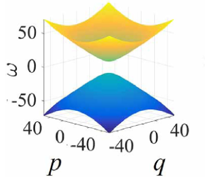
Figure 7: The spectrum (4.66), produced by the linearization of the simplified SOC equations (4.63) and (4.64), plotted for $\Omega=10$, The spectrum clearly displays the presence of the finite bandgap (4.67) (source: Li et al. (2017)).

Actually, branches of the full spectrum (4.52) cover (eliminate) the finite bandgap (4.67), but this happens at very large values of $k$. This fact implies that, in the framework of the full system, the gap solitons will start decay through emission of radiation, but the emission rate will be exponentially small.

IV.7 Nonlinear optical couplers emulating the spin-orbit coupling (SOC)

IV.7.1 A spatiotemporal coupler emulating SOC in two dimensions

In the spirit of possibilities to emulate matter-wave phenomenology by means of optics and vice versa, a realization of the stabilization mechanism for 2D optical solitons, operating similar to that in Eqs. (4.48), (4.49) and (4.55), was proposed by Kartashov et al. (2015). The model is based on the consideration of the spatiotemporal propagation of light in a dual-core planar waveguide (coupler) with the Kerr nonlinearity acting in each core. In this case, amplitudes of the electromagnetic waves in the two cores of the coupler, $q_{1}$ and $q_{2}$, form a pseudospinor wave function which obeys the following system of equations.

$$i\frac{\partial q_{1}}{\partial\xi}=-\frac{1}{2}\left(\frac{\partial^{2}}{\partial\eta^{2}}+\frac{\partial^{2}}{\partial\tau^{2}}\right)q_{1}-\left|q_{1}\right|^{2}q_{1}-\left(C+i\delta\frac{\partial}{\partial\tau}\right)q_{2}-\beta q_{1},$$ (136)

$$i\frac{\partial q_{2}}{\partial\xi}=-\frac{1}{2}\left(\frac{\partial^{2}}{\partial\eta^{2}}+\frac{\partial^{2}}{\partial\tau^{2}}\right)q_{2}-\left|q_{2}\right|^{2}q_{2}-\left(C+i\delta\frac{\partial}{\partial\tau}\right)q_{1}+\beta q_{2},$$ (137)

Here $\xi$ is the scaled propagation distance, $\eta$ are $\tau$ are, respectively, the transverse and temporal coordinates, the group-velocity-dispersion (GVD) coefficient (assuming the anomalous sign of the GVD), effective diffraction coefficient, and Kerr coefficients are scaled to be $1$, $C$ is the real coupling coefficient, $\delta$ accounts for the temporal dispersion of the coupling, and $\beta$ determines the phase-velocity mismatch between the cores. This system is similar to Eq. (4.55), with the SOC terms represented by the first derivatives acting on the single coordinate, $\tau$, which is sufficient for the stabilization of spatiotemporal solitons in this system (solitons which feature self-trapping in both temporal and spatial directions in optical media are often called “light bullets”, as was first proposed by Silberberg (1990)). As concerns the dispersion relation for the linearized system of Eqs. (4.69) and (4.70), the respective plane-wave solutions are sought for as

$$q_{1,2}\sim\exp\left(ik\eta-i\omega\tau+ib\xi\right),$$ (138)

cf. Eqs. (4.51) and (4.66). The result is the relation between the real propagation constant $b$, transverse wavenumber $k$ and frequency $\omega$:

$$b=-\frac{1}{2}\left(k^{2}+\omega^{2}\right)\pm\sqrt{(C+\delta\cdot\omega)^{2}+\beta^{2}},$$ (139)

which is similar to Eq. (4.54).

IV.7.2 The parity-time ($\mathcal{PT}$) symmetric SOC-emulating optical-coupler model

Another possibility for the emulation of 2D SOC by means of spatiotemporal propagation of optical waves in planar dual-core couplers with the Kerr nonlinearity was elaborated by Sakaguchi and Malomed (2016). That setting makes it possible to combine SOC, nonlinearity, and the effect known as parity-time ($\mathcal{PT}$) symmetry.

Settings featuring the $\mathcal{PT}$ symmetry may be considered as ones designed at the border between conservative and dissipative systems. This concept had appeared in quantum mechanics as a possibility to realize non-Hermitian Hamiltonians which, nevertheless, produce purely real spectra of energy eigenvalues (see a review of the topic by Bender (2007), and a book by Moiseyev (2011)). The basic idea is to construct a Hamiltonian which includes a complex potential $U(\mathbf{r})$, whose real and imaginary parts are, respectively, even and odd functions of coordinates, $\mathbf{r=}\{x,y,z\}$:

$$U(\mathbf{r})=U_{\mathrm{even}}(\mathbf{r})+iU_{\mathrm{odd}}(\mathbf{r}),$$ (140)

hence the potential satisfies the symmetry condition

$$U(-\mathbf{r})=U^{\ast}(\mathbf{r})$$ (141)

(recall $\ast$ stands for the complex conjugate). A well-known examples is the 1D potential,

$$U(x)=U_{0}x^{2}\left(ix\right)^{\varepsilon},$$ (142)

which, with $U_{0}>0$ and real $\varepsilon$, obviously satisfies condition (4.74). It is known that each eigenvalue of the HO potential, to which potential (4.75) reduces at $\varepsilon=0$, continues, at all values $\varepsilon>0$, as a real positive eigenvalue, monotonously increasing with the growth of $\varepsilon$. On the other hand, at $\varepsilon<0$ the $\mathcal{PT}$ symmetry suffers breaking through a chain of bifurcations at which pairs of adjacent eigenvalues collide and become complex (unphysical) with the increase of $|\varepsilon|$. The last surviving eigenvalue is one originating at $\varepsilon=0$ from the HO’s ground state. The complex potential (4.75) gives rise to no real eigenvalues at $\varepsilon<-1$.

While experimental realization of the $\mathcal{PT}$ symmetry in quantum mechanics is a challenge, it can be readily emulated in optics, as reviewed by Makris et al. (2011). Indeed, the paraxial light propagation in the spatial domain obeys the equation of the Schrödinger type for local amplitude $u(z,x)$ of the electromagnetic field. In the planar waveguide, its scaled form is

$$i\frac{\partial u}{\partial z}+\frac{1}{2}\frac{\partial^{2}u}{\partial x^{2}}-U_{\mathrm{even}}(x)u=iU_{\mathrm{odd}}(x)u,$$ (143)

where an even real function $-U_{\mathrm{even}}(x)$ represents a spatially even modulation of the local refractive index, while an odd real function $U_{\mathrm{odd}}(x)$ represents a globally balanced distribution of local gain ($U_{\mathrm{odd}}(x)>0$) and loss ($U_{\mathrm{odd}}(x)<0$). This setup was used by Rüter et al. (2010) in the experimental realization of the $\mathcal{PT}$ symmetry in optics. Although the model represented by Eq. (4.76) is a dissipative one, it shares basic properties, such as the possibility of generating a purely real spectrum of eigenvalues, with conservative systems.

While the concept of the $\mathcal{PT}$ symmetry is a linear one, its realization in optics suggests to combine it with the Kerr nonlinearity of optical media. This possibility opens the way to creation of a large variety of $\mathcal{PT}$-symmetric solitons (see reviews by Konotop, Yang, and Zezyulin, 2016, and Suchkov et al. 2016).

The blend of SOC and $\mathcal{PT}$ symmetry, proposed Sakaguchi and Malomed (2016), is based on the use of a dual-core waveguide (coupler). This setup is natural, as couplers provide optical platforms for the emulation of both the SOC (see Eqs. (4.69), (4.70)) and $\mathcal{PT}$ symmetry, provided that the two cores of the coupler carry mutually balanced gain and loss (Driben and Malomed, 2011; Alexeeva et al., 2012). The $\mathcal{PT}$-symmetric coupler may be designed in the 2D form as well (Burlak and Malomed, 2013).

The “blended” model is based on the following system of NLS equations for amplitudes $u_{1}$ and $u_{2}$ of the electromagnetic waves in the coupled cores:

$$i\left(u_{1}\right)_{z}+\frac{1}{2}\left[\left(u_{1}\right)_{tt}+\left(u_{1}\right)_{xx}\right]-\delta\cdot\left(u_{2}\right)_{x}+u_{2}+\left|u_{1}\right|^{2}u_{1}=i\Gamma u_{1},$$ (144)

$$i\left(u_{2}\right)_{z}+\frac{1}{2}\left[\left(u_{2}\right)_{tt}+\left(u_{2}\right)_{xx}\right]+\delta\cdot\left(u_{1}\right)_{x}+u_{1}+\left|u_{2}\right|^{2}u_{2}=-i\Gamma u_{2}.$$ (145)

Here, $z$ is the propagation distance, $x$ and $t$ are the transverse and temporal coordinates, assuming the anomalous GVD, real $\Gamma>0$ represents real gain and loss coefficients in the two cores, while the coefficients of the Kerr nonlinearity, paraxial diffraction, and inter-core coupling are scaled to be $1$. Unlike Eqs. (4.69) and (4.70), this system does not include dispersion of the coupling, while the pseudo-SOC terms $\mp\delta\cdot\left(U_{2,1}\right)_{x}$ account for “skewness” of the coupling in the transverse direction, assuming that the layer separating the guiding cores has an oblique structure, as schematically shown in Fig. 8: roughly speaking, light couples point $x$ in the top core to point $x+\delta$ in the bottom one.

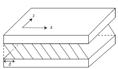
Figure 8: A scheme of the planar coupler with an oblique layer between the guiding cores, which realizes the model based on Eqs. (4.77) and (4.78). Amplitudes of the electromagnetic waves in the top and bottom cores are $u_{2}$ and $u_{1}$, respectively. Slanted lines designate the skew of the intermediate layer, measured by transverse shift $\delta$ (source: Sakaguchi and Malomed, 2016).

The dispersion relation for the plane-wave solutions of the linearized version of Eqs. (4.77) and (4.78), looked for as

$$u_{1,2}\sim\exp\left(ikx-i\omega t+ibz\right)$$ (146)

(cf. Eq. (4.71)), is

$$\left(b+\frac{1}{2}\omega^{2}+\frac{1}{2}k^{2}\right)^{2}=1-\Gamma^{2}+\left(\delta\cdot k\right)^{2},$$ (147)

cf. Eq. (4.72). This dispersion relation demonstrates that the $\mathcal{PT}$ symmetry holds at $\Gamma\leq 1$, i.e., under the condition that the gain-loss coefficient is smaller than the inter-core coupling constant, which is scaled to be $1$. Further consideration of Eq. (4.80) demonstrates that it gives rise to solutions for propagation constant $b$ taking values in the semi-infinite band:

$$b<b_{\max}\equiv\left\{\begin{array}[]{c}(1/2)\left[\delta^{2}+\left(1-\Gamma^{2}\right)\delta^{-2}\right],~{}\mathrm{at}~{}~{}\delta^{2}>\sqrt{1-\Gamma^{2}},\\ \sqrt{1-\Gamma^{2}},~{}\mathrm{at}~{}~{}\delta^{2}<\sqrt{1-\Gamma^{2}}.\end{array}\right.$$ (148)

Accordingly, solitons may exist in the remaining semi-infinite bandgap, i.e., at $b>b_{\max}$ (Sakaguchi and Malomed, 2016).

IV.7.3 Stabilization of 1D solitons in the SOC-emulating skewed coupler with the quintic self-focusing

A similar, although effectively one-dimensional, scheme, based on the dual-core system with the skewed coupling between the cores and the quintic self-focusing carried by the cores, was elaborated by Shamriz, Chen, and Malomed (2020b). As mentioned above, the quintic self-focusing plays the special role in 1D equations of the NLS type, leading to the critical collapse in that case. Accordingly, the one-dimensional pseudo-SOC makes it possible to suppress the critical collapse driven by the quintic self-attraction, and thus stabilize solitons in the system.

The corresponding system of coupled one-dimensional NLS equations is

$$iu_{z}+\frac{1}{2}u_{xx}+|u|^{4}u+v-\delta\cdot v_{x}=0,$$ (149)

$$iv_{z}+\frac{1}{2}v_{xx}+|v|^{4}v+u+\delta\cdot u_{x}=0,$$ (150)

where $\delta$ has the same meaning as in Eqs. (4.77) and (4.78). Looking for solutions to the linearized system of Eqs. (4.83) and (4.84) as

$$\left\{u,v\right\}\sim\exp\left(ikz+iqx\right),$$ (151)

one derives the dispersion relation between the propagation constant ($k$) and transverse wavenumber, $q$:

$$k=-(1/2)q^{2}\pm\sqrt{1+\delta^{2}q^{2}}.$$ (152)

The spectrum determined by Eq. (4.85) includes bandgaps, i.e., intervals of $k$ in which the linear plane waves do not exist, hence they may be populated by solitons, in the framework of the full nonlinear system. In the case of $\delta^{2}>1$ (when the pseudo-SOC is strong enough), it is the semi-infinite main bandgap,

$$k>k_{\max}\equiv\frac{\delta^{4}+1}{2\delta^{2}}.$$ (153)

Formal values of $q$ in the main bandgap are complex, hence solitons populating it have oscillatory tails.

In the case of $\delta^{2}<1$, there is an additional finite annex bandgap, adjacent to the main one:

$$1<k<\frac{\delta^{4}+1}{2\delta^{2}}.$$ (154)

In the annex bandgap, formal values of $q$ are purely imaginary, hence the respective solitons have tails monotonously decaying at $|x|\rightarrow\infty$. Further details can be found in the paper by Shamriz, Chen, and Malomed (2020b)

IV.8 Three-dimensional SOC systems

The most ambitious objective of the work with systems of GP equations incorporating SOC terms is to use such terms to predict a possibility of the stabilization of 3D solitons. This problem was addressed by Zhang et al. (2015) in the work which made use of the scaled GP system, including SOC of the Weyl type and the attractive cubic nonlinearity, written for the two-component pseudospinor wave function $\Psi=\left\{\psi_{+},\psi_{-}\right\}$:

$$\left[i\partial_{t}+\frac{1}{2}\nabla^{2}+i\lambda\nabla{\small\cdot}{\bm{\sigma}}+\left(\begin{array}[]{cc}|\psi_{+}|^{2}+\eta|\psi_{-}|^{2}&0\\ 0&|\psi_{-}|^{2}+\eta|\psi_{+}|^{2}\end{array}\right)\right]\Psi=0.$$ (155)

Here $\lambda$ is the SOC coefficient, $\mathbf{\sigma}=\left\{\sigma_{x},\sigma_{y},\sigma_{z}\right\}$ is the vector of the Pauli matrices, and the coefficient of the cubic self-attraction is scaled to be $1$, while $\eta$ is the relative strength of the cross-attraction between the components of the wave function. The energy corresponding Eq. (4.88) is written as

$$E=E_{\mathrm{kin}}+E_{\mathrm{int}}+E_{\mathrm{pseudospin}}~{},\,$$ (156)

$$E_{\mathrm{kin}}=\frac{1}{2}\int\int\int\left|\nabla\Psi\right|^{2}dxdydz,~{}$$ (157)

$$E_{\mathrm{int}}=-\frac{1}{2}\int\int\int\left(|\psi_{+}|^{4}+|\psi_{-}|^{4}+2\eta|\psi_{+}\psi_{-}|^{2}\right)dxdydz\,,$$ (158)

$$E_{\mathrm{pseudospin}}=-i\lambda\int\int\int\Psi^{{\dagger}}\left(\nabla{\small\cdot}{\bm{\sigma}}\right)\Psi dxdydz,$$ (159)

cf. Eqs. (4.59) – (4.63).

While the system represented by Eqs. (4.88) - (4.92) is a fully three-dimensional one, it was demonstrated by Sherman et al. (2020) that 3D solitons may be stabilized by SOC terms which, by themselves, are two-dimensional, including only derivatives $\partial_{x}$ and $\partial_{y}$. The respective system of 3D GP equations for the two-component wave function with the quasi-2D SOC terms is

$$\left[i\partial_{t}+\frac{1}{2}\nabla^{2}+i\sum_{j=x,y}\lambda_{j}\sigma_{j}\partial_{j}+\left(\begin{array}[]{cc}\left|\psi_{+}\right|^{2}+\gamma|\psi_{-}|^{2}&0\\ 0&\left|\psi_{-}\right|^{2}+\gamma|\psi_{+}|^{2}\end{array}\right)+\Omega\sigma_{z}\right]\Psi,$$ (160)

where real coefficients $\lambda_{x}$ and $\lambda_{y}$ represent the SOC strengths. The 3D GP system (4.93) is a straightforward generalization of its 2D counterpart written above in the form of Eq. (4.55), which provides for the stabilization of 2D solitons by means of the quasi-1D SOC terms.

In the 2D setting, the addition of the SOC terms to the system of GP equations with the cubic attraction makes it possible to create absolutely stable solitons, which play the role of the otherwise missing ground state of the system (Sakaguchi, Li, and Malomed, 2014). The difference of the 3D systems with SOC terms, such as (4.88) and (4.93), is that they can maintain metastable solitons, while the true ground state remains missing in the system, as the cubic attraction is too strong (supercritical, as mentioned above) in the 3D case.

V Stabilization of 3D and 2D fundamental solitons and vortices by linear trapping potentials

V.1 The formulation of the problem

In the appropriately normalized form, the three-dimensional GP equation for the mean-field wave function $\psi$ of the self-attracting BEC trapped in the axisymmetric (but not necessarily fully isotropic) HO potential, with the scaled planar and axial strengths $1$ and $\Omega^{2}$, is obtained from Eq. (4.9):

$$i\psi_{t}+\frac{1}{2}\nabla^{2}\psi+|\psi|^{2}\psi-\frac{1}{2}\left[\left(x^{2}+y^{2}\right)+\Omega^{2}z^{2}\right]\psi=0.$$ (161)

Coefficient $\Omega$ determines the aspect ratio between the trapping lengths imposed by the HO potential in the $\left(x,y\right)$ plane and long the $z$ axis:

$$\mathrm{a.r.}\equiv\sqrt{\Omega}$$ (162)

The 2D version of Eq. (5.1) corresponds to dropping coordinate $z$ in Eq. (5.1). Actually, the 2D limit corresponds to very strong confinement of the BEC along $z$, with $\mathrm{a.r.}\rightarrow\infty$, imposed by $\Omega^{2}\rightarrow\infty$. The opposite limit, with $\mathrm{a.r.}\rightarrow 0$, corresponds to $\Omega^{2}\rightarrow 0$. Up to rescaling, it represents “tubular” quasi-one-dimensional solitons with embedded vorticity, maintained by a cigar-shaped (strongly prolate) trap, which are stable states (Salasnich, Malomed and Toigo, 2007).

It is relevant to mention that, while the trapping magnetic, optical, or combined potentials indeed had the HO (parabolic) form in a majority of experimental works with ultracold gases, the creation of a 3D confining optical potential $U(r)$ in the form approximated by the infinitely deep spherical box, with

$$U_{\mathrm{box}}\left(r\equiv\sqrt{x^{2}+y^{2}+z^{2}}\right)=\left\{\begin{array}[]{c}0,r<r_{0},\\ +\infty,r>r_{0},\end{array}\right.$$ (163)

was reported by Gaunt et al. (2013) and Navon et al. (2013). A 2D version of the box potential (5.3) was created and used by Hueck et al. (2018).

Equation (5.1) conserves the energy,

$$E=\frac{1}{2}\int\int\int\left[\left(\left|\psi_{x}\right|^{2}+\left|\psi_{y}\right|^{2}+\left|\psi_{z}\right|^{2}\right)+(x^{2}+y^{2}+\Omega^{2}z^{2})|\psi|^{2}-|\psi|^{4}\right]dxdydz,$$ (164)

along with the norm and $z$-component of the angular momentum, which are defined, respectively, as per Eqs. (4.13) and (4.14). In cylindrical coordinates $\left(r,\theta,z\right)$, defined as per Eq. (4.10), stationary states of Eq. (5.1), with chemical potential $\mu$ and integer vorticity $S$, are looked for as

$$\psi=R(r,z)\exp\left(iS\theta-i\mu t\right),$$ (165)

(cf. Eq. (4.11)), with real function $R(r,z)$ satisfying the stationary equation,

$$\frac{\partial^{2}R}{\partial r^{2}}+\frac{1}{r}\frac{\partial R}{\partial r}+\frac{\partial^{2}R}{\partial z^{2}}+\left(2\mu-\frac{S^{2}}{r^{2}}-r^{2}-\Omega^{2}z^{2}\right)R-2R^{3}=0,$$ (166)

cf. Eq. (4.12). The 2D version of Eq. (5.6) is obtained by dropping terms $\partial^{2}R/\partial z^{2}$ and $-\Omega^{2}z^{2}R$.

Stability of the numerically found stationary solutions is inspected through computation of eigenvalues $\lambda$ of small perturbations, introduced by looking for solutions to Eq. (5.1) in the form of

$$\psi(x,y,z,t)=[R(r,z)+u(r,z)\exp(\lambda t+iL\theta)+v^{\ast}(r,z)\exp(\lambda^{\ast}t-iL\theta)]\exp\left(iS\theta-i\mu t\right),$$ (167)

where $\left(u,v\right)$ are eigenmodes of infinitesimal perturbations with integer values of azimuthal index $L$, and $\ast$ stands, as above, for the complex conjugate. The substitution of ansatz (5.7) in Eq. (5.1) and linearization with respect to the perturbations leads to the system of BdG equations,

$$\left(i\lambda+\mu\right)u+\frac{1}{2}\left[\frac{\partial^{2}}{\partial r^{2}}+\frac{1}{r}\frac{\partial}{\partial r}+\frac{\partial^{2}}{\partial z^{2}}-\frac{(S+L)^{2}}{r^{2}}u-r^{2}-\Omega^{2}z^{2}\right]u+R^{2}(v+2u)=0,$$ (168)

$$\left(-i\lambda+\mu\right)v+\frac{1}{2}\left[\frac{\partial^{2}}{\partial r^{2}}+\frac{1}{r}\frac{\partial}{\partial r}+\frac{\partial^{2}}{\partial z^{2}}-\frac{(S-L)^{2}}{r^{2}}v-r^{2}-\Omega^{2}z^{2}\right]v+R^{2}(u+2v)=0,$$ (169)

which have to be solved with b.c. demanding that $u(r)$ and $v(r)$ decay exponentially at $r\rightarrow\infty$ and $\left|z\right|\rightarrow\infty$, and decay as $r^{\left|S\pm L\right|}$ at $r\rightarrow 0$.

In physical units, assuming a weak isotropic trap with frequency $2\pi\times 10$ Hz, into which a gas of ⁷Li atoms is loaded (for this atomic species, the application of FR makes it possible to induce the attractive interactions, with scattering length $a_{s}\simeq-0.1$ nm (Bradley et al. 1995)), a typical radius of the vortex is $\sim 10$ $\mathrm{\mu}$m, a characteristic time scale is $\sim 0.1$ s, and a typical number of atoms in a stable vortex, $\sim 10^{5}$, corresponds to values $\sim 10$ of the dimensionless norm.

V.2 Stability of 2D fundamental solitons and vortices

Systematic results for the existence and stability of 2D solitons (fundamental and vortical ones), produced by numerical solutions of the 2D versions of Eqs. (5.1), (5.6), and (5.8), were reported by Mihalache et al. (2006) and Carr and Clark (2006), following an earlier work by Alexander and Bergé (2002). Families of solutions, with $S=0$ (the fundamental solitons) and $S=1$ and $2$ (the solitons with embedded vorticity), in the form of dependences of their chemical potentials on the 2D norm,

$$N_{\mathrm{2D}}=\int\int\left|\psi\left(x,y\right)\right|^{2}dxdy\equiv 2\pi\int_{0}^{\infty}R^{2}(r)rdr$$ (170)

(see Eq. (5.5)), are displayed in the left panel of Fig. 9, which also indicates their stability. In the limit of $\mu\rightarrow-\infty$, the norm of the fundamental solitons is approaching the TS value, $N_{\mathrm{TS}}\approx 5.85$ (see Eq. (3.12)). For $S=1$ and $S=2$, the respective limit values correspond to the TSs with embedded vorticity, which were introduced (actually, as unstable states) by Kruglov and Vlasov (1985), and Kruglov et al. (1988). In particular, for the TS with $S=1$, this value is

$$N_{\mathrm{TS}}^{(S=1)}\approx 24.1.$$ (171)

It was demonstrated by Qin, Dong, and Malomed (2016) that, for all $S\geq 1$, the TS norm is accurately predicted by formula

$$N_{\mathrm{TS}}^{(S)}\approx 4\sqrt{3}\pi S$$ (172)

(in particular, for $S=1$ Eq. (5.11) yields $N_{\mathrm{TS}}^{(S=1)}\approx\allowbreak 21.8$, with a relative difference $\approx 9.5\%$ from numerical value (5.10)). The fact that the norm of all solitons approaches the TS value in the limit of $\mu\rightarrow-\infty$ is explained by the circumstance that the width of these solitons shrinks $\sim 1/\sqrt{-\mu}$, and for very narrow solitons the effect of the trapping potential becomes negligible, i.e., they may be indeed considered as TSs in the free space.

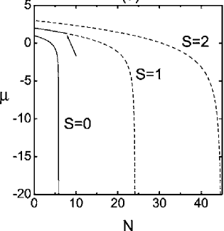
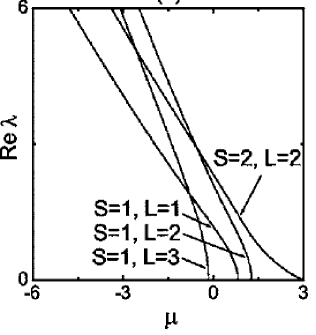
Figure 9: The left panel: dependence $\mu(N)$ of the chemical potential of 2D solitons trapped in the HO potential (see Eqs. (5.1) and (5.6)), with embedded vorticity $S=0,1,2$, on their norm, defined as per Eq. (5.9) ($S=0$ pertains to the fundamental solitons). Continuous and dashed lines represent stable and unstable (sub)families. The solitons with $S=0$ and $S=2$ are, severally, completely stable and unstable. For the family with $S=1$, the tilted arrow indicates the boundary between stable ($N<7.79$) and unstable ($7.79<N<N_{\mathrm{TS}}^{(S=1)}\approx 24.1$) subfamilies. The right panel displays dependences of the instability growth rates, $\mathrm{Re}\lambda$, on $\mu$ for the same families, as obtained from numerical solution of the 2D version of Eqs. (5.8). The curves are labeled by integer azimuthal index $L$ of the perturbation eigenmode, defined as per Eq. (5.7) (source: Mihalache et al., 2006).

Further, Fig. 9 demonstrates that the family of the fundamental solitons is entirely stable, in agreement with the prediction of the VK criterion, $d\mu/dN<0$, which obviously holds for all branches shown in the left panel of Fig. 9. Thus, even an arbitrarily weak trapping potential makes the family of the fundamental TSs, which is fully unstable in the free space, a completely stable one. This finding is explained by the fact that, a seen in Fig. 9, the trap lifts the above-mentioned norm degeneracy of the TSs in the free space. As a results, all the solitons drop their norms to values below the collapse threshold, $N<N_{\mathrm{TS}}$, making the onset of the collapse impossible.

For the family of the trapped solitons with $S=1$, the VK criterion is not sufficient for securing their stability. The point is that this criterion indeed protects the vortex states against collapsing, but not against spontaneous splitting into fragments. The instability spectrum, i.e., dependences of the instability growth rate on the chemical potential $\mu$ of the vortex solitons with $S=1$ and $2$, is displayed in the right panel of Fig. 9. The plot is produced by numerical solution of the two-dimensional variant of BdG equations (5.8). As a result, it is found that the solitons with $S=1$ are stable in the interval of norms

$$0<N<N_{\mathrm{crit}}^{(S=1)}\approx 7.79\approx 0.32N_{\mathrm{TS}}^{(S=1)}$$ (173)

(cf. Eq. (5.10)). In the remaining part of their existence region, viz., at

$$7.79<N<24.1,$$ (174)

the solitons with $S=1$ are unstable against splitting, in accordance with the fact that the dominant instability mode in Fig. 9 corresponds to $L=2$ in Eq. (5.7). Instability growth rates which account for the splitting instability are complex ones. Accordingly, they form a quartet of the form

$$\lambda_{1,2,3,4}=\pm\mathrm{Re}(\lambda)\pm i\mathrm{Im}(\lambda),$$ (175)

with two independent signs $\pm$, which represent the so-called Hamiltonian-Hopf bifurcation (van der Meer, 1990). In terms of the chemical potential, the stability region (5.12) corresponds to

$$\mu_{\mathrm{crit}}\approx 1.276<\mu<\mu_{\max}\equiv 2.$$ (176)

Here, $\mu_{\max}=1+S$ is commonly known quantum-mechanical energy eigenvalue of the 2D isotropic HO potential, which correspond to the limit of $N\rightarrow 0$, i.e., to Eq. (5.1) replaced by its linearized version.

The numerical analysis demonstrates that irreversible splitting of the unstable vortex solitons into fragments actually takes place in a part of region (5.12), namely,

$$10.30<N<N_{\mathrm{TS}}^{(S=1)}\approx 24.1.$$ (177)

Because the norm of the fragments produced by the splitting of the vortex in interval (5.16) exceeds the above-mentioned TS norm for the fundamental soliton, $N_{\mathrm{TS}}^{(S=0)}\approx 5.85$ (see Eq. (3.12)), each fragment eventually develops the intrinsic collapse. On the other hand, in the narrower interval,

$$7.79<N<10.30,$$ (178)

which occupies $\approx 10\%$ of the existence region, $0<N<$ $N_{\mathrm{TS}}^{(S=1)}\approx 24.1$, the norm of the fragments falls below the collapse threshold. For this reason, unstable vortex solitons with the norm falling in interval (5.17) periodically splits in two fragments and recombines back, as shown in Fig. 10. The corresponding dynamical pattern keeps its vorticity, while the relative loss of its norm in the course of the evolution from $t=0$ to $t=240$ is $\approx 1.9\times 10^{-3}$, which corroborates the robustness of the pattern.

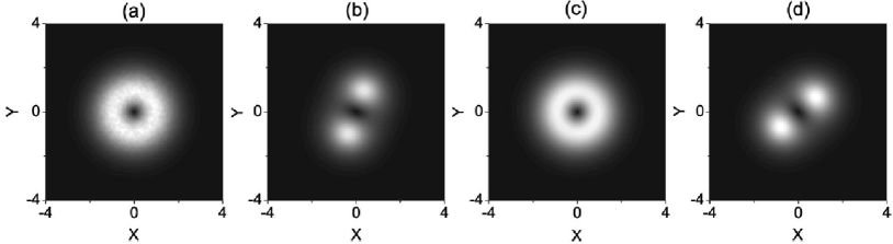
Figure 10: Density profiles of the 2D solitons with vorticity $S=1$ trapped in the HO potential, with initial norm $N=8.476$, which belongs to interval (5.16). In this case, simulations of Eq. (5.1), starting from a numerically exact solution of stationary equation (5.6) with $\mu=1.2$, give rise to a periodic sequence of splittings and recombinations. Shown here are the density prfiles as $t=0$ (a), $t=100$ (b), $t=140$ (c), and $t=180$ (d) (source: Mihalache et al., 2006).

All the vortex solitons with $S\geq 2$ are completely unstable solutions, in the framework of Eq. (5.1) with the self-attractive cubic nonlinearity. Indeed, the entire existence region for these states, $\mu\leq 3$, is covered, in the right panel of Fig. 46, by the splitting-instability branch corresponding to $L=2$.

V.3 Variational and numerical results for 3D fundamental and vortical solitons trapped in the HO potential

Results for 3D fundamental (zero-vorticity) solitons, produced by numerical solution of Eqs. (5.6) and (5.8), are quite simple. They are presented in Fig. 11 by means of $\mu(N)$ curves (similar to the 2D situation, shown in Fig. 9) for three values of the anisotropy parameter, $\Omega=10$, $1$, and $0.1$, which correspond, respectively, to the oblate, spherically isotropic, and prolate trapping potential in Eq. (5.1). As well as in the 2D case, the stability of the fundamental solitons exactly obeys the VK criterion (the negative slope), $d\mu/dN<0$; however, unlike the 2D situation, the $\mu(N)$ curves in Fig. 11 contain segments with negative and positive slopes, only the former ones being stable. The norm of the soliton family attains it maximum at the point where the two segments connect.

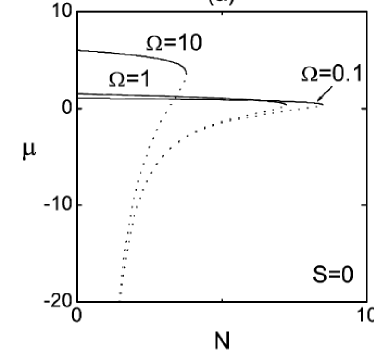
Figure 11: Dependences of the chemical potential on the norm for families of 3D fundamental (zero-vorticity) solitons, produced by the numerical solution of Eq. (5.6) for three different values of the HO-trap parameter $\Omega$. Solid and dashed segments of the curves represent, respectively, stable and unstable soliton subfamilies, in exact agreement with the VK stability criterion, $d\mu/dN<0$ (source: Malomed et al., 2007).

Families of 3D vortex solutions to Eq. (5.6) were found in a numerical form by Adhikari (2001), and stability eigenvalues for some vortices with $S=1$ were computed by Saito and Ueda (2002). A rather accurate analytical approximation for these families is provided by the variational method, which was developed by Malomed et al. (2007). To apply the VA to Eq. (5.6), note that this equation can be derived from the Lagrangian,

$$L=\int_{0}^{\infty}rdr\int_{0}^{+\infty}dz\left[R_{z}^{2}+R_{r}^{2}+\left(\frac{S}{r}\right)^{2}R^{2}-2\mu R^{2}+\left(r^{2}+\Omega^{2}z^{2}\right)R^{2}-R^{4}\right].$$ (179)

A natural 3D ansatz for vortex states with integer winding number $S\geq 0$ is (cf. Eq. (4.32))

$$R(r,z)=Ar^{S}\exp\left[-r^{2}/\left(2\rho^{2}\right)-z^{2}/\left(2h^{2}\right)\right],$$ (180)

where $A,\rho$, and $h$ are free parameters. The 3D norm (4.13) of this ansatz is

$$N=\left(\pi^{3/2}S!\right)M,~{}M\equiv A^{2}\rho^{4}h,$$ (181)

and the substitution of the ansatz in Lagrangian (5.18) yields the corresponding effective Lagrangian (written here for $S=1$, as all the states with $S\geq 2$ are completely unstable):

$$L_{\mathrm{eff}}=\frac{\sqrt{\pi}}{8}M\left(-4\mu+\frac{1}{h^{2}}+\frac{4}{\rho^{2}}+4\rho^{2}+\Omega^{2}h^{2}-\frac{M}{2\sqrt{2}\rho^{2}h}\right).$$ (182)

Then, values of variational parameters $A$, $h$, and $\rho$ in ansatz (5.19) are predicted by the Euler-Lagrange equations,

$$\partial L_{\mathrm{eff}}/\partial\left(A,h,\rho\right)=0.$$ (183)

In particular, the last equation in system (5.22) takes a simple form,

$$M=8\sqrt{2}h\left(1-\rho^{4}\right),$$ (184)

which predicts that the vortex state may only exist if it is narrow enough in the radial direction, with $\rho<1$, which is a natural consequence of the presence of the trapping potential.

The results for the vortex solitons with $S=1$ are displayed by means of $\mu(N)$ curves, along with their counterparts produced by the numerical solution of Eq. (5.6), in the left panel of Fig. 49. It is seen that the VA, based on ansatz (5.19), provides sufficiently accurate predictions, in comparison to the numerical findings, at all values of the anisotropy parameter $\Omega$.

The stability of the vortex-soliton families with $S=1$ was identified from the numerical solution of the BdG equations (5.8). The results show in the right panel of Fig. 12 that, similar to the 2D case (cf. Fig. 46), the VK criterion is only necessary but not sufficient for the stability of the vortex modes, as it determines the stability only against the collapse, which is represented by real eigenvalues $\lambda$, but not against the splitting, which is accounted for by a quartet of complex eigenvalues, in the general form given by Eq. (5.14). It is worthy to note that the stability interval of the norm is much wider for the prolate trap (with $\Omega=0.1$), $0<N<N_{\max}\approx 20.347$, and for the isotropic one (with $\Omega=1$), $0<N<N_{\max}\approx 15.023$, than for the oblate trap with $\Omega=10$, for which the stability interval is $0<N<N_{\max}\approx 5.947$.

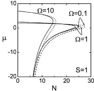
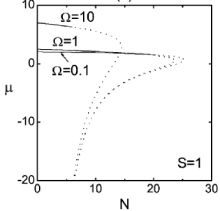
Figure 12: The left panel: dependences $\mu(N)$ for 3D solitons with embedded vorticity $S=1$, as predicted by the VA based on ansatz (5.19) and Euler-Lagrange equations (5.21)-(5.23) (dashed lines), and as obtained from the numerical solution of Eq. (5.6) (solid lines). The dependences are presented for three values of the anisotropy parameter $\Omega$. The right panel: the same numerically produced $\mu(N)$ curves, separated into stable (solid) and unstable (dashed) segments, as predicted by the numerical solution of the BdG equations (5.8) (source: Malomed et al., 2007).

The predictions for the stability of the 3D solitons produced by the solution of the BdG equations (5.8) were completely confirmed by direct simulations of Eq. (5.1) for perturbed evolution (Malomed et al., 2007). In particular, the robustness of stable vortices with $S=1$ is illustrated by Fig. 13, which demonstrates that the stable donut-shaped vortex soliton is able to absorb strong disturbance and restore its unperturbed shape.

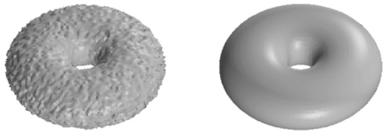
Figure 13: Self-cleaning of a stable 3D vortex soliton (“donut”) with $S=1$ in the isotropic model ($\Omega=1$ in Eq. (5.1)) after the application of a random initial perturbation at the amplitude level of $10\%$. The left and right panels display, respectively, the shape of the perturbed vortex at the initial moment, $t=0$, and at $t=120$. The unperturbed vortex soliton has chemical potential $\mu=2$ and norm $N=12.55$ (source: Malomed et al., 2007).

V.4 Stable 2D two-component solitons with hidden vorticity

Proceeding to the consideration of two-component systems under the action of the self-attractive nonlinearity and trapping potential, it is straightforward to investigate stability of vortex solitons with equal wave functions of both components (Yakimenko, Zaliznyak, and Lashkin, 2009). A more intriguing possibility is to seek for stable two-component solitons with HV (hidden vorticity), which are built of components carrying opposite winding numbers, $S_{1,2}=\pm S$ (Brtka, Gammal, and Malomed, 2010).

In this case, the system of nonlinearly coupled GP equations for wave functions $\psi_{1,2}$ of the two components is

$$i\frac{\partial\psi_{1}}{\partial t}=\left[-\frac{1}{2}\left(\frac{\partial^{2}}{\partial x^{2}}+\frac{\partial^{2}}{\partial y^{2}}\right)-\left(|\psi_{1}|^{2}+\beta\left|\psi_{2}\right|^{2}\right)+\frac{1}{2}\left(x^{2}+y^{2}\right)\right]\psi_{1},$$ (185a)

$$i\frac{\partial\psi_{2}}{\partial t}=\left[-\frac{1}{2}\left(\frac{\partial^{2}}{\partial x^{2}}+\frac{\partial^{2}}{\partial y^{2}}\right)-\left(|\psi_{2}|^{2}+\beta\left|\psi_{1}\right|^{2}\right)+\frac{1}{2}\left(x^{2}+y^{2}\right)\right]\psi_{2},$$ (186)

The system is assumed to be fully symmetric, with strengths of the self-attraction in each component and HO potential scaled to be $1$, like in the single-component GP equation (5.1), while $\beta$, that may be both positive and negative, is the relative strength of the interaction between the components (attraction for $\beta>0$ and repulsion for $\beta<0$). In this notation, the collapse threshold for the norm of each component of the symmetric ($\psi_{1}=\psi_{2}$) soliton with $S_{1,2}=\pm 1$ follows from Eq. (5.10):

$$N_{\mathrm{TS}}^{(S=\pm 1)}\approx 24.1\left(1+\beta\right)^{-1}.$$ (187)

HV states are stationary solutions of Eqs. (5.24), written in the polar coordinates as

$$\psi_{1}=\exp\left(-i\mu t+iS\theta\right)\phi(r),\psi_{2}=\exp\left(-i\mu t-iS\theta\right)\phi(r),$$ (188)

with $S\geq 1$ and real function $\phi(r)$ determined by the same radial equation as in the case of the state with the explicit vorticity (i.e., with identical phase terms $S\theta$ in both components, rather than $\pm S\theta$ in Eq. (5.26)):

$$\mu\phi=-\frac{1}{2}\left(\frac{d^{2}\phi}{dr^{2}}+\frac{1}{r}\frac{d\phi}{dr}-\frac{S^{2}}{r^{2}}-r^{2}\right)-\left(1+\beta\right)\phi^{3}.$$ (189)

While the density profile of the HV modes is the same as of the usual 2D vortex solitons, up to obvious rescaling $\phi\rightarrow\left(1+\beta\right)^{-1/2}\phi$ (provided that $\beta>-1$), the stability is different. To address this point, a perturbed HV solution is looked for as

$$\psi_{1,2}(r,t)=[R(r)+u_{1,2}(r)\exp\left(\lambda t+iL\theta\right)+v_{1,2}^{\ast}(r)\exp\left(\lambda^{\ast}t-iL\theta\right)]\exp\left(-i\mu t\pm iS\theta\right),$$ (190)

where $+S$ and $-S$ correspond to $\psi_{1}$ and $\psi_{2}$, respectively, and $L$ is an integer azimuthal index, cf. Eq. (5.7). The substitution of this expression in Eqs. (5.24) and the linearization with respect to small perturbations $\left(u_{1,2},v_{1,2}\right)$ leads to the respective BdG equations. Then, the numerical solution of the BdG equations produces the stability chart for $S=1$, displayed in Fig. 14, in which the stability area for the HV states is shown in the plane of $\left(N,\beta\right)$ ($N$ is defined as the norm of one component). For $S\geq 2$, all the HV states are completely unstable.

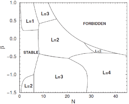
Figure 14: The stability chart for the HV (hidden-vorticity) 2D solitons with $S_{1,2}=\pm 1$ (see Eq. (5.26)) in the plane of $\left(N,\beta\right)$, produced by the numerical solution of Eqs. (5.24) and the respective BdG equations for small perturbations. Here $N$ is the norm of one component of the unperturbed state (the total norm is $2N$). In domains labeled by different values of $L$ the HV states are unstable against perturbation modes with the respective value of azimuthal index $L$, see Eq. (5.28). In the “forbidden” area, bounded by curve $N\approx 24.1/\left(1+\beta\right)$ (see Eq. (5.25)), vortex solitons with $S=1$ do not exist (source: Brtka, Gammal, and Malomed 2010).

In other parts of the plane displayed in Fig. 14, instability domains dominated by perturbation eigenmodes with different values of azimuthal index $L$ are identified, as per the results of Brtka, Gammal, and Malomed (2010). It is worthy to note an essential difference from the instability for the usual vortex solitons which, as shown above in Fig. 9, is always dominated by the perturbation eigenmode with $L=2$, hence the unstable vortex spontaneously splits in two fragments (Fig. 10). Figure 14 demonstrates that the eigenmode with $L=2$ remains dominant for the HV solitons at, roughly speaking, $|\beta|<0.5$; on the other hand, $L=1$, $3$ and $4$ may be the azimuthal indices of the leading perturbation eigenmode at $|\beta|>0.5$. When, in particular, the leading unstable perturbation has $L=1$, it does not split the HV soliton. Instead, the weak instability slowly deforms it into a rotating crescent-shaped mode, as shown in Fig. 52 (eventually, this mode implodes under the action of the intrinsic collapse).

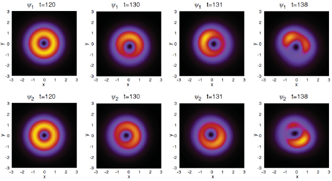
Figure 15: The slowly developing instability of the HV soliton in the case when the dominant perturbation eigenmode has azimuthal index $L=1$ (see Fig. 14). The top and bottom rows of panels display the distribution of the densities in two components of the HV state at indicated moments of time, as produced by simulations of Eqs. (5.24) with $\beta=0.5$. The unperturbed HV soliton has the norm (in each component) $N=7.5$ and chemical potential $\mu=0.83$ (source: Brtka, Gammal, and Malomed 2010).

On the other hand, the instability corresponding to the dominant eigenmodes with $L=3$ or $4$ splits the HV soliton into three or four fragments, respectively (later, the fragments are destroyed by the intrinsic collapse). In particular, the instability dominated by $L=4$ is very strong, leading to fast splitting of the HV soliton, as shown in Fig. 16.

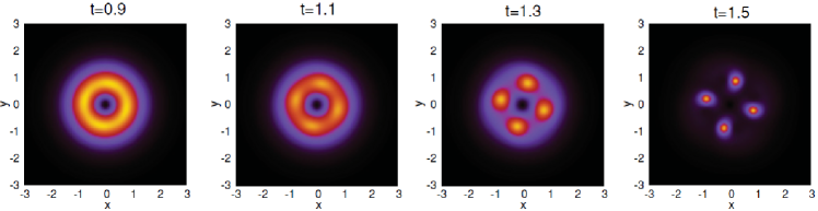
Figure 16: The rapidly developing instability of the HV soliton in the case when the dominant perturbation eigenmode has azimuthal index $L=4$ (see Fig. 14). The set of panels display identical distributions of the density in both components at indicated moments of time. The results were produced by simulations of Eq. (5.24) with $\beta=-0.5$. The unperturbed HV soliton has the norm (in each component) $N=34.1$ and chemical potential $\mu=-0.2$ (source: Brtka, Gammal, and Malomed 2010).

VI Nonlinear trapping potentials

The trapping potentials considered in the previous chapter provide the traditional method for maintaining and stabilizing localized states, which, by itself, applies independently of the presence of nonlinearity in the system. Nonlinear potentials, induced by spatial modulation of the local strength of the cubic or other nonlinearity, offer a completely different method for the creation of self-trapped states (quasi-solitons). An efficient implementation of the latter method was proposed by Borovkova et al. (2011a,b), in the form of the self-repulsive cubic term with the coefficient growing fast enough from the center to periphery, as per Eqs. (4.28) and (4.31) or (4.32). This scheme offers options for the creation of various localized states that would not exist or would be unstable without the use of nonlinear potentials. Although experimental realization of the scheme has not yet been reported, many possibilities of its use have been explored theoretically. In particular, an essential asset of the theoretical work in this direction is that, although it is naturally based on numerical methods, many important results may be obtained in an analytical form, approximately or exactly.

VI.1 The basic setting

The basic model providing self-trapping of various 2D and 3D modes in the effective nonlinear trapping potential is (Borovkova et al. (2011a,b)),

$$i\psi_{t}+\frac{1}{2}\nabla^{2}\psi-\sigma(r)|\psi|^{2}\psi=0,$$ (191)

where $r$ is the radial coordinate in the 2D or 3D space in which Eq. (6.1) is written, and the local self-defocusing coefficient, $\sigma(r)>0$, grows from the center ($r=0$) to periphery ($r\rightarrow\infty$). This equation conserves the total norm defined as per Eq. (4.13),

$$N_{\mathrm{3D}}=\int\int\int dxdydz\left|\psi\right|^{2},N_{\mathrm{2D}}=\int\int dxdy\left|\psi\right|^{2},$$ (192)

the Hamiltonian (cf. Eq. (4.15)),

$$H_{\mathrm{3D}}=\frac{1}{2}\int\int\int dxdydz\left[\left|\nabla\psi\right|^{2}+\sigma(r)|\psi|^{4}\right]$$ (193)

(or its counterpart in the 2D case), and the vectorial angular momentum, given above by Eq. (4.16). In the 2D case, the norm, Hamiltonian, and $z$-component of the angular momentum are produced by obvious reduction of the 3D expressions.

Stationary states with real chemical potential $\mu$ are sought for as solutions to Eq. (6.1) in the form of

$$\psi\left(r,t\right)=\exp\left(-i\mu t\right)w(\mathbf{r}),$$ (194)

where $\mathbf{r}$ is the set of coordinates in the respective 2D or 3D space, and function $w$ (generally, a complex one) satisfies the stationary equation,

$$\mu w+\frac{1}{2}\nabla^{2}w-\sigma(\mathbf{r})|w|^{2}w=0.$$ (195)

The fundamental condition necessary for the existence of physically relevant self-trapped states produced by Eq. (6.5) is the convergence at $r\rightarrow\infty$ of the integral expression (6.2) which defines the norm of the state. In particular, if $\sigma(r)$ grows asymptotically at $r\rightarrow\infty$ as

$$\sigma_{\mathrm{asympt}}(r)=\sigma_{0}r^{\alpha}$$ (196)

with $\sigma_{0}>0$ and $\alpha>0$, it is easy to identify the convergence condition by means of the TF approximation, which neglects term $(1/2)\nabla^{2}w$ in Eq. (6.4) (a rigorous justification of the application of the TF to models of the present type was developed by Malomed and Pelinovsky (2015)). In this approximation, the solution is obvious,

$$\left(|w|^{2}\right)_{\mathrm{TF}}=\mu/\sigma(r)$$ (197)

(it exists for $\mu>0$), and the substitution of this in Eq. (6.2) immediately shows that the integral converges under the condition

$$\alpha>D.$$ (198)

In fact, condition (6.8) secures the self-trapping for localized modes of all types, i.e., not only fundamental ones, but also states with an intrinsic structure, such as embedded vorticity (Borovkova et al. (2011a)). It is relevant to mention that the same condition also secures the convergence of the integral which defines Hamiltonian (6.3).

In the model with the asymptotic form (6.6) of the spatially modulated local nonlinearity, the asymptotic solution including the term given by Eq. (6.7) and the first post-TF correction, produced by term $(1/2)\nabla^{2}w$ at $r\rightarrow\infty$, is

$$w_{\mathrm{TF-corrected}}(r)\approx\sqrt{\frac{\mu}{\sigma_{0}}}r^{-\alpha/2}+\frac{1}{4\sqrt{\mu\sigma_{0}}}\left[\frac{\alpha}{2}\left(\frac{\alpha}{2}-\left(D-2\right)\right)-m^{2}\right]r^{-\alpha/2-2}$$ (199)

(the term $\sim m^{2}$ appears in the 2D case, representing the effect of the vorticity with integer winding number $m$, see Eq. (6.11) below).

Expression (6.9) shows that the TF approximation yields the asymptotically exact expression for the soliton’s tail at $r\rightarrow\infty$, as the first correction to it is negligibly small, hence the convergence condition, given by Eq. (6.8), is always correct. Further, it is relevant to stress that stationary equation (6.5) with the nonlinearity-modulation profile (6.6) is nonlinearizable: while the solution’s tail decays at $r\rightarrow\infty$, its asymptotic form, determined by the TF approximation (6.7) and (6.9), cannot be found from the linearization of Eq. (6.5), unlike the usual situation for nonlinear equations in the free space.

VI.2 Typical examples of the self-trapped modes

Basic results illustrating the realization of the concept of the effective nonlinear trapping potential were reported by Borovkova et al. (2011a), who considered 2D version of Eq. (6.1) with

$$\sigma(r)=1+r^{\alpha},$$ (200)

whose asymptotic form complies with expression (6.6) (the 1D version of the model was also considered in that work). Along with the fundamental 2D solitons, their counterparts with embedded vorticity $m$ were considered too, with Eqs. (6.4) and (6.5) replaced by

$$\psi\left(r,t\right)=\exp\left(-i\mu t+im\theta\right)w(r),$$ (201)

$$\mu w+\frac{1}{2}\left(\frac{d^{2}w}{dr^{2}}+\frac{1}{r}\frac{dw}{dr}-\frac{m^{2}}{r^{2}}w\right)-\left(1+r^{\alpha}\right)w^{3}=0,$$ (202)

where $\theta$ is the angular coordinate. In this case, the substitution of the TF approximation (6.6), with $\sigma(r)$ taken as per Eq. (6.10), yields the prediction for the total norm of the fundamental ($m=0$) solitons, which is relevant for all dimensions, $D=1$, $2$, and $3$:

$$N_{\mathrm{TF}}=\frac{2\pi^{D}\mu}{\alpha\sin\left(\pi D/\alpha\right)}.$$ (203)

In particular, this expression provides the convergent norm precisely under condition (6.8).

Typical examples of radial profiles of stationary states, produced by the numerical solution of Eq. (6.12) with $m=0$, $1$, and $2$, are displayed in Fig. 17, and families of the respective solution families, characterized by dependences $N(\mu)$ and $N(\alpha$), are shown in Fig. 55. The latter plot includes the TF prediction (6.13) for $m=0$, showing that the TF approximation is quite accurate at all values of $\alpha$. Note also that the linear dependence of $N_{\mathrm{TF}}$ on $\mu$, predicted by Eq. (6.13), is in perfect agreement with the linear line for $m=0$ in Fig. 18(a).

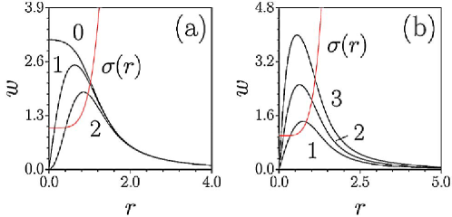
Figure 17: (a) Radial profiles of self-trapped solutions produced by the numerical solution of Eq. (6.12) with $\alpha=5$ and a fixed chemical potential, $\mu=10$, for vorticities $m=0$, $m=1$, and $m=2$. (b) Vortex states for $\alpha=5$, $m=1$ and $\mu=5$, $10$, and $20$ (curves 1, 2, and 3, respectively). The red curve shows the respective nonlinearity-modulation profile, defined as per Eq. (6.10) (source: Borovkova et al., 2011a).

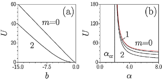
Figure 18: (a) The norm of 2D self-trapped states (denoted $U$, instead of $N$) produced by the numerical solution of Eq. (6.12), vs. the chemical potential (denoted $-b$, instead of $\mu$), for $\alpha=5$ and two values of the vorticity, $m=0$ and $2$. (b) Dependences of the 2D norm on power $\alpha$ from Eq. (6.10) for a fixed chemical potential, $\mu=10$, and three values of the vorticity: $m=0$, $1$, and $2$. Value $\alpha_{\mathrm{cr}}=2$ is determined by Eq. (6.7), with the norm diverging at $\alpha\geq\alpha_{\mathrm{cr}}$. The red curve shows the analytical prediction for $m=0$ produced by the TF approximation in the form of Eq. (6.13) (source: Borovkova et al., 2011a).

VI.3 Stability of the self-trapped states

Stability of the 2D self-trapped states produced by Eq. (6.12) against small perturbations was investigated by Borovkova et al. (2011(a)) by means of the numerical solution of the respective BdG equations, cf. Eqs. (5.8). As a result, it was concluded that the entire family of fundamental solitons, with $m=0$, is stable, in accordance with the fact that the respective $N(\mu)$ dependence in Fig. 18(a) obeys the anti-VK criterion, $dN/d\mu>0$, which is a necessary stability condition for families of localized states supported by the self-repulsive nonlinearity (on the contrary to the opposite VK criterion per se, in the case of self-attraction), as shown by Sakaguchi and Malomed (2010). In the notation adopted Fig. 6.2(a), the anti-VK criterion means $dU/db<0$.

Unlike the fundamental self-trapped states, ones with embedded vorticity tend to be vulnerable to instability, their stabilization being possible for sufficiently steep nonlinearity-modulation profiles in Eq. (6.10); in particular, the entire family of the vortices with $m=1$ was found by Borovkova et al. (2011a) to be completely stable at $\alpha\geq 8$, being only partly stable at smaller $\alpha$ (e.g., for $-\mu>30$ at $\alpha=5$).

Direct simulations demonstrate that instability of the vortex mode with $m=1$ expels the vortex’ pivot from the central position, and drives its drift towards periphery. As shown in Fig. 19(a), the pivot eventually vanishes in the peripheral area. The angular momentum of the original vortex state is also ousted to the periphery where, in actual numerical simulations, it is eliminated by a numerical absorber providing stability of the numerical scheme. In the case when a double vortex with $m=2$ is unstable, small perturbations may split it in two unitary vortices, one staying as a stable one with $m=1$ at the center, while the other one spontaneously drifting to the periphery, where it vanishes eventually. The latter scenario of the instability development is shown in Fig. 19(b).

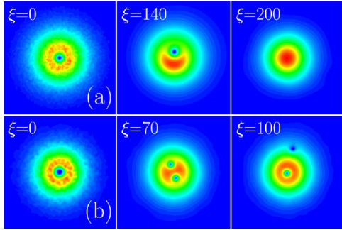
Figure 19: (a) The development of the drift instability of the vortex state with $m=1$ and $\mu=3$, produced by simulations of Eq. (6.1) with the nonlinearity-modulation profile (6.10), where $\alpha=3.5$. Colors denote values of the local density, $\left|\psi\left(x,y,t\right)\right|^{2}$, with variable $t$ replaced by $\xi$. (b) The same for the splitting-drift instability of the double vortex, with $m=2$, $\mu=20$, and $\alpha=4$ (source: Borovkova et al., 2011a).

VI.4 Exact, approximate, and numerical results for the anti-Gaussian spatial-modulation profile

VI.4.1 The formulation and analytical findings

Stronger results for self-trapped states supported by the spatial modulation of the cubic repulsive term were reported by Borovkova et al. (2011b) in the framework of Eq. (6.1) with a very steep (anti-Gaussian) modulation profile (cf. the algebraic one in Eq. (6.10)):

$$\sigma(r)=\exp\left(\alpha r^{2}\right).$$ (204)

Note that the scaling invariance of Eq. (6.1) with $\sigma(r)$ taken as per Eq. (6.14) implies that the solutions actually depend not separately on $\alpha$ and $\mu$, but solely on the ratio, $\mu/\alpha$.

A remarkable finding is that the 2D version of Eqs. (6.1) and (6.5) with $\sigma(r)$ taken as per Eq. (6.14) admits a particular exact solution for the self-trapped mode with embedded vorticity $m=1$:

$$\psi=\frac{\alpha}{\sqrt{2}}r\exp\left(-i\mu t+i\theta-\frac{\alpha}{2}r^{2}\right),\mu=2\alpha$$ (205)

(the exact solution is available for the single value of $\mu$, as written in Eq. (6.15)). As concerns the asymptotic form of the solution’s tail at $r\rightarrow\infty$, it is determined by the balance of the cubic and gradient terms in Eq. (6.5):

$$w(r)=\left[\frac{\alpha}{\sqrt{2}}r+\frac{2\mu-\alpha\left(D+2\right)}{2\sqrt{2}\alpha r}+\mathcal{O}\left(\frac{1}{r^{3}}\right)\right]\exp\left(-\alpha r^{2}/2\right).$$ (206)

This asymptotic solution is a universal one, as, apart from the correction $\mathcal{O}\left(1/r^{3}\right)$, it does not depend on $\mu$, nor on the presence of embedded vorticity $m$, and only the correction $\sim 1/r$ depends on the spatial dimension, $D$. Vanishing of the latter term in the case of $D=2$, $\mu=2\alpha~{}$agrees with the existence of the exact solution given by Eq. (6.15).

Similar to the case of modulation profile (6.10), the one represented by Eq. (6.14) makes equation (6.5) nonlinearizable, as the tail solution (6.16), although it vanishes at $r\rightarrow\infty$, cannot be found in the correct form, unless the nonlinear term is kept in the analysis. On the other hand, the approximation leading to Eq. (6.16) is different from the TF approximation, which was used above to derive expression (6.9), as the gradient term is negligible in the latter case.

In any spatial dimension $D$, fundamental solitons (with $m=0$) produced by Eqs. (6.5) and (6.14) can be very accurately approximated by the variational method. To this end, one notes that the 2D ($D=2$) or 3D ($D=3$) Lagrangian of Eq. (6.5) with real field $w(r)$ is

$$L_{w}=\frac{1}{2}\int_{0}^{\infty}\left[\mu w^{2}-\frac{1}{2}\left(\frac{dw}{dr}\right)^{2}-\frac{1}{2}\sigma(r)w^{4}\right]r^{D-1}dr.$$ (207)

A natural ansatz approximating the fundamental soliton is

$$w(r)=A\exp\left(-\frac{\alpha}{2}r^{2}\right),$$ (208)

with the norm

$$N=\left(\pi/\alpha\right)^{D/2}A^{2},$$ (209)

where amplitude $A$ is a free variational parameter.

The substitution of ansatz (6.18) in Lagrangian (6.29) yields the following effective Lagrangian, in which $A^{2}$ is expressed in terms of $N$, by means of relation (6.19):

$$L_{\mathrm{2D}}=\frac{1}{4\pi}\left(\mu-\frac{\alpha}{2}\right)N-\frac{\alpha}{8\pi^{2}}N^{2},$$ (210)

$$L_{\mathrm{3D}}=\frac{1}{8\pi}\left(\mu-\frac{3\alpha}{4}\right)N-\frac{\alpha^{3/2}}{16\pi^{5/2}}N^{2}.$$ (211)

Finally, the Euler-Lagrange equation, $\partial L/\partial N=0$, predicts the following relation between the norm and chemical potential:

$$N=\left(\pi/\alpha\right)^{D/2}\left(\mu-D\alpha/4\right).$$ (212)

Numerically found dependences $N(\alpha)$ for the fundamental solitons are indistinguishable from the VA prediction (6.21), in both cases $D=2$ and $3$ (Borovkova et al. 2011b).

A two-component extension of Eqs. (6.1), in the form of

$$i\left(\psi_{1,2}\right)_{t}+\frac{1}{2}\nabla^{2}\psi_{1,2}-\sigma(r)\left(|\psi_{1,2}|^{2}+C\left|\psi_{2,1}^{2}\right|\right)\psi=0,$$ (213)

with an XPM coefficient $C>0$, was elaborated by Kartashov et al. (2011).

VI.4.2 Vortices and rotary structures

Shapes of fundamental and vortical self-trapped modes created by the anti-Gaussian modulation profile (6.14) are quite similar to those shown above in Fig. 17 for profile (6.10). However, results for the stability of vortices are different: unlike the above model, where vortices even with the lowest winding number, $m=1$, tend to be unstable, see Fig. 56(a), all the 2D vortex states supported by the anti-Gaussian profile (6.14) are completely stable, as well as all the fundamental modes in all dimensions (Borovkova et al., 2011b). Alternation of stability and instability commences from $m=2$, as shown in Fig. 20. In case the vortex modes with $m=3$ and $3$ are unstable, they do not start drift to $r\rightarrow\infty$, unlike what is shown above in Fig. 19(a); instead, they spontaneously split in robust rotating sets of two or three unitary vortices, as seen in Fig. 21.

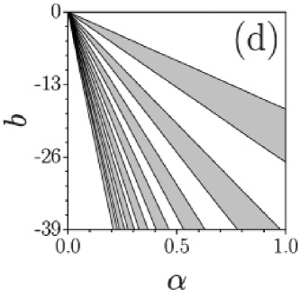
Figure 20: Self-trapped vortex modes with $m=2$, generated by Eqs. (6.1) and (6.14), are stable and unstable in white and shaded sectors of the parametric plane $\left(\alpha,b\equiv b\equiv-\mu\right)$. Note that the scaling invariance of the underlying equation implies that all boundaries of the stability sectors are strict straight lines, $\mu/\alpha=\mathrm{const}$, as seen in the figure (source: Borovkova et al., 2011b).

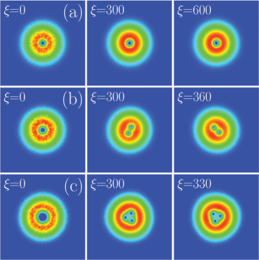
Figure 21: (a) Relaxation to the stationary state of a perturbed stable vortex solution of Eqs. (6.1) and (6.17) with $m=2$ and $\mu=17$. (b) Spontaneous splitting of an unstable vortex with $m=2$ and $\mu=11$ into a steadily rotating pair of unitary vortices. (c) The splitting of the unstable vortex with $m=3$ and $\mu=9$ into a rotating triplet of unitary vortices. In this figure $\xi\equiv t$ (source: Borovkova et al., 2011b).

The same 2D model, based on Eq. (6.1) with the modulation profile given by Eq. (6.14), also supports stable rotational motion of a single vortex with the pivot shifted off the center, as well of clusters composed of several vortices (Kartashov et al., 2017). The respective GP equation, written in the reference frame rotating with angular velocity $\omega$, is written as

$$i\psi_{t}+\frac{1}{2}\nabla^{2}\psi+i\omega\left(x\frac{\partial}{\partial y}-y\frac{\partial}{\partial x}\right)\psi-\sigma(r)|\psi|^{2}\psi=0.$$ (214)

($\omega>0$ corresponds to the counter-clockwise rotation).

A snapshot of the density distribution in a stable vortex moving along a circular trajectory is displayed in Fig. 22(a). Further, separated vortex and antivortex, with winding numbers $\pm 1$, may form a non-rotating dipole, as shown in Fig. 22(b), and a non-rotating quadrupole built of alternating vortices and antivortices is shown in Fig. 22(d) (generally speaking, vortex dipoles and quadrupoles are subject to weak instability in the absence of rotation (Möttönen et al., 2005)). In the usual confined BEC, vortex-antivortex dipoles were experimentally created by Freilich et al. (2010).

When the vortex dipole is unstable, its evolution may expel one vortex to periphery, where it eventually disappears, while the remaining antivortex falls onto the center, thus converting the unstable dipole into a stable stationary vortex with the unitary topological charge. This instability-development scenario resembles the one displayed above in Fig. 19(b). The application of the rotation ($\omega\neq 0$ in Eq. (6.23)) helps to stabilize vortex-antivortex clusters. Simultaneously, Figs. 22(c), (e), and (f) demonstrate that dipoles, quadrupoles, and sextupoles (a set of three vortices alternating with three antivortices), which are symmetric complexes in the absence of the rotation, are deformed by the rotation. The deformation is caused by an effective Coriolis force acting with opposite signs on individual vortices and antivortices. In particular, Fig. 22(c) shows that this force pushes the vortex and antivortex, belonging to the dipole, towards $r=0$ and $r\rightarrow\infty$, respectively, and Fig. 22(f) shows that the sextupole, which has a symmetric hexagonal shape at $\omega=0$, is deformed into a triangular structure. Finally, if $\omega$ is too large, the fast rotation destroys the clusters.

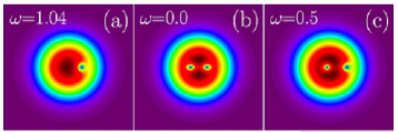
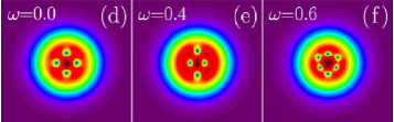
Figure 22: (a): A snapshot of the density distribution in a 2D vortex with $m=1$ and norm $N=58.4$, which performs orbiting motion in the framework of Eqs. (6.23) and (6.14) with $\alpha=0.5$ and $\omega=1.04$. Panels (b) and (d): the density distribution in stationary spatially symmetric dipole and quadrupole vortex-antivortex clusters, produced by Eqs. Eqs. (6.23) and (6.14) with $\alpha=0.5$, $\omega=0$, and $\mu=10$. (c) and (e): The same clusters stabilized and simultaneously deformed by the rotation. (f) The density distribution in a stable rotating sextupole with $\alpha=0.5$, $\mu=20$, built as a cluster of three vortices alternating with three antivortices. Each panel shows an area in the $\left(x,y\right)$ plane of size $\left(-5,+5\right)$ in each direction (source: Kartashov et al., 2017).

Additional results for 2D and 3D fundamental and vortex solitons were produced by means of numerical methods, in similar models with more sophisticated (specially devised) profiles of the spatial modulation of the strength of the self-repulsive cubic nonlinearity (Tian et al. 2012; Wu et al. 2013). Another direction of the work was the analysis of a similar model with the local quintic self-repulsive nonlinearity (Zeng and Malomed, 2012).

VI.4.3 A discrete 2D model with the exponential nonlinearity-modulation profile

It is relevant to mention that a discrete version of the models considered here was elaborated by Kevrekidis et al. (2015). The corresponding lattice (discrete) NLS equation, with the 2D discrete coordinates $\left(m,n\right)$ is

$$i\frac{d\psi_{mn}}{dt}=-\varepsilon\left(\psi_{m+1,n}+\psi_{m-1.n}+\psi_{m,n+1}+\psi_{m,n-1}-4\psi_{m,n}\right)+\sigma\left(m,n\right)\left|\psi_{m,n}\right|^{2}\psi_{m,n}~{},$$ (215)

cf. Eqs. (2.163) and (6.1), with the exponential profile of the spatial modulation of local nonlinearity,

$$\sigma\left(m,n\right)=\exp\left(2\left(|m|+|n|\right)\right),$$ (216)

cf. Eq. (6.14). Various species of 2D discrete solitons supported by Eqs. (6.24) and (6.25) have been constructed, and their stability has been investigated. Among them were two types of discrete vortex solitons, viz., OS-centered vortex crosses, whose shape is similar to that displayed above in Fig. 24, and IS-centered vortex squares).

VI.5 Gyroscope solitons (vortex tori) in 3D

Full consideration of the structure and dynamics of fundamental and vortical solitons in the 3D version of Eq. (6.1) with the modulation profile defined by Eq. (6.14), where $\alpha=1/2$ is fixed by means of rescaling, was presented by Driben et al. (2014a). The respective stationary equation (6.5) for modes with embedded vorticity $S$, introduced as per Eq. (6.11) with real function $w\left(r,z\right)$, takes the following form, in cylindrical coordinates $\left(r,z\right)$:

$$\mu w=-\frac{1}{2}\left(\frac{\partial^{2}}{\partial r^{2}}+\frac{1}{r}\frac{\partial}{\partial r}-\frac{S^{2}}{r^{2}}\right)w+\exp\left(\frac{1}{2}\left(r^{2}+z^{2}\right)\right)w^{3}.$$ (217)

As shown above, the VA based on Eqs. (6.18), (6.19), and (6.21) with $D=3$ produces a very accurate prediction for the family of fundamental solitons, with $S=0$. For 3D solitons with embedded vorticity $m\geq 1$, the VA is less accurate. However, in this case quite relevant is the TF approximation. Indeed, neglecting the derivative terms in Eq. (6.26), one obtains

$$w_{\mathrm{TF}}^{2}=\begin{array}[]{c}0,~{}\mathrm{at}~{}r^{2}<m^{2}/\left(2\mu\right),\\ \left[\mu-S^{2}/\left(2r^{2}\right)\right]\exp\left(-\frac{1}{2}\left(r^{2}+z^{2}\right)\right),~{}\mathrm{at}~{}r^{2}>S^{2}/\left(2\mu\right).\end{array}$$ (218)

The TF approximation (6.27) produces the norm of the vortex state in the form of

$$N_{\mathrm{TF}}(\mu)=4\left(2\pi\right)^{3/2}\mu\exp\left(-\frac{S^{2}}{4\mu}\right)\int_{0}^{\infty}\frac{e^{-R}RdR}{4R+S^{2}/\mu}$$ (219)

(here, the integral factor should be computed numerically).

Numerically found shapes of typical stable 3D solitons with vorticities $S=0$, $1$, and $2$ are displayed in Fig. 23 (because of their shape, the solitons with $S\neq 0$ are often called vortex tori, alias 3D vortex rings). It was found that all the states with $S=0$ and $S=1$ are stable, while ones with $S=2$ and $3$ feature alternating stability and instability zones. Generic examples of the dynamics of stable and unstable solitons are presented in Fig. 24. It is seen that a stable soliton cleans itself of a strong initial perturbation, while unstable ones with $S=2$ and $3$ spontaneously split in rotating clusters of two and three unitary vortices, respectively.

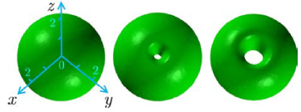
Figure 23: Typical examples of stable 3D self-trapped modes produced by the numerical solution of Eq. (6.26) with $\mu=16$ and $S=0$, norm $N=246.1$ (left), $S=1$, $N=225.2$ (central), and $S=2$, $N=191.7$. The modes are displayed by means of isosuraces, $\left|w\left(x,y,z\right)\right|^{2}=3$ (source: Driben et al., 2014a).

Figure 24: Generic examples of the perturbed dynamics of 3D solitons with embedded vorticity $S=1$ in the top row (a stable vortex torus with $\mu=16$; the plots are shown at $t=0$, $t=230$, $t=310$); $S=2$ in the middle row (an unstable vortex torus with $\mu=13$, shown at $t=0$, $t=230$, $t=310$); and $S=3$ (an unstable vortex torus with $\mu=25$, shown at $t=0$, $t=165$, $t=180$). $N=191.7$. The top and middle rows display density isosurfaces $\left|\psi\left(x,y,z\right)\right|=2.5$, and bottom one displays $\left|\psi\left(x,y,z\right)\right|=3$ (source: Driben et al., 2014a).

Families of the completely stable solitons with $S=0$ and $1$ are characterized by dependences $N(\mu)$ shown in Fig. 25. It is clearly seen that the VA for the fundamental solitons with $S=0$ and the TF approximation for ones with $S=1$ produce the $N(\mu)$ lines which are indistinguishable from their numerically generated counterparts.

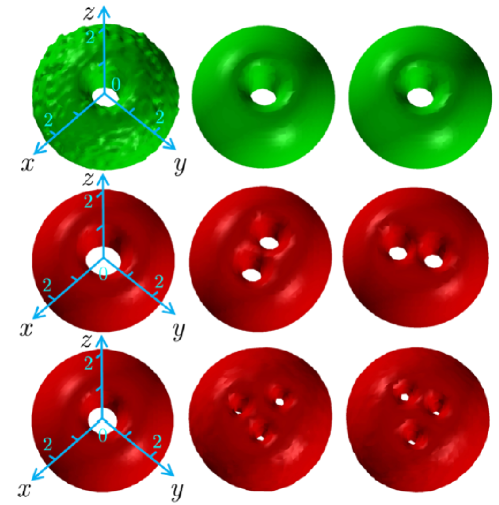
Figure 25: Black lines show the norm of the fundamental solitons (a) and ones with $S=1$ (b) vs. their chemical potential. Chains of green dots represent the VA prediction for the fundamental solitons, given by Eq. (6.21) with $D=3$, and the TF prediction for $S=1$, given by Eq. (6.28). The empty circle in (a) and bold red dot in (b) correspond, respectively, to the left plot in Fig. 60, and the top row in Fig. 24 (source: Driben et al., 2014a).

The stable 3D solitons with embedded vorticity demonstrate macroscopic dynamics resembling that of mechanical gyroscopes. An example if displayed in Fig. 63. To generate it, Eqs. (6.1) and (6.14) with $\alpha=1/2$ was simulated, with the input taken as the stable soliton with $S=1$, shown in Figs. 60 and 61, to which a torque is applied at $t=0$, multiplying the soliton’s wave function by the phase factor

$$T=\exp\left(i\beta z\tanh\left(x/x_{0}\right)\right),$$ (220)

with real $\beta$. This factor adds a nonzero component $M_{y}$ of the angular momentum (see Eq. (4.16)). In particular, if the unperturbed vortex is taken in the form defined by the TF approximation, as per Eqs. (6.11), (6.27), and (6.28), the momentum produced by torque (6.29) is

$$M_{y}=\frac{\beta}{2x_{0}}\left[N-\left(2\pi\right)^{3/2}\left(\mu-\frac{S^{2}}{4}\right)\right],$$ (221)

while the the momentum of the unperturbed vortex soliton is

$$M_{z}=SN.$$ (222)

Then, as it may be expected, the application of the torque to the gyroscope sets it in the state of precession, as shown in Fig. 63. This dynamical regime corresponds to the total angular momentum with components (6.31) and (6.30).

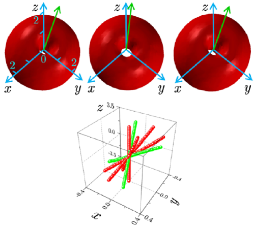
Figure 26: The gyroscopic precession of the 3D vortex soliton (torus) with $S=1$ and $\mu=16$, initiated by the application of torque (6.29) with $\beta=4$ and $x_{0}=5$. The plots are produced by simulations of Eqs. (61.) and (6.14) with $\alpha=1/2$. Three images in the top row correspond to times $t=90$, $90.8$, and $91.5$. Time $\Delta t=1.5$ between the first and third images is equal to the precession period. Green arrows indicate the corresponding orientations of the axle of the precessing gyroscope. The bottom plot shows a set of instantaneous orientations of the axle, the green ones corresponding to those displayed in the top row (source: Driben et al., 2014a).

VI.6 Hopfions: 3D solitons with two independent topological charges

As shown above in Fig. 23, the density distribution in 3D solitons with embedded vorticity $m$ is shaped as a torus (“donut”). An additional possibility is to impose intrinsic twist, characterized by integer number $s$, onto the torus, in an attempts to create self-trapped modes carrying two independent topological charges. States of such a type were originally predicted in the Faddeev-Skyrme model (Faddeev, 1976; Faddeev and Niemi, 1997), based on a set of three real scalar fields. Soliton-like states in that system realize the Hopf map, $R^{3}\rightarrow S^{2}$, therefore they are called hopfions.

In usual settings, the creation of hopfions requires, at the minimum level, two complex components (Sutcliffe and Manton, 2004; Sutcliffe, 2007). A unique possibility offered by the 3D equation (6.1) with the modulation profile (6.14) is to predict single-component stable hopfions (Kartashov et al., 2014). The respective stationary solutions were looked for, in the cylindrical coordinates $\left(r,\theta,z\right)$, as

$$\psi=\exp\left(-i\mu t+im\theta\right)\,w\left(r,z\right),$$ (223)

with complex field $w$ satisfying equation

$$\mu w=-\frac{1}{2}\left(\frac{\partial^{2}}{\partial r^{2}}+\frac{1}{r}\frac{\partial}{\partial r}-\frac{m^{2}}{r^{2}}\right)w+\exp\left(\frac{1}{2}\left(r^{2}+z^{2}\right)\right)|w|^{2}w.$$ (224)

Examples of hopfions with sets of topological numbers $\left(s=1,m=0\right)$, $\left(s=1,m=1\right),$ $\left(s=1,m=1\right)$, and $\left(s=1,m=2\right)$, found as numerical stationary solutions of Eq. (6.1), are shown, from the top to bottom, in the left images of Fig. 27. Solutions with $s>1$ do not exist (note that the solution with $S=0$ and $s=1$, i.e., zero overall vorticity, exists, as shown in the top row of Fig. 27). Further, the evolution of the hopfions, displayed in Fig. 27, demonstrates that all the hopfions with $\left(s=1,m=0\right)$ are stable, ones with $\left(s=m=1\right)$ may be stable or unstable, depending on their chemical potential (or norm), and all the states with $\left(s=1,m\geq 2\right)$ are completely unstable against spontaneous breakup (the results for the hopfions with $s=-1$ are the same).

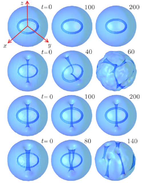
Figure 27: Four rows display, from left to right, the distribution of the density in hopfion stationary solutions of Eq. (6.33), and their evolution, governed by the underlying equations (6.1) and (6.14) (with $\alpha=1/2$). Parameters (twist number $s$ of the intrinsic torus, overall vorticity $m$, and chemical potential $\mu$) are, from the top to bottom: $\left(s=1,m=0,\mu=15\right)$, $\left(s=1,m=1,\mu=16\right)$, $\left(s=1,m=1,\mu=22\right)$, and $\left(s=1,m=2,\mu=22\right)$. Snapshots of the evolving hopfions are taken at moments of time indicated in the figure. In the second row, the density isosurface is drawn as $\left|\psi\left(x,y,z\right)\right|^{2}=0.2$, and in all others is it $\left|\psi\left(x,y,z\right)\right|^{2}=1$ (source: Kartashov et al., 2014).

Shapes of the hopfions displayed in Fig. 27 suggest that the respective solution to Eq. (6.26) may be approximated by the following ansatz, proposed by Kartashov et al. (2014) (assuming $s\geq 0$ and $m\geq 0$):

$$w=A\left[\left(r-R\right)+iz\right]^{s}r^{m}\exp\left[-\frac{1}{2}\left(r^{2}+z^{2}\right)\right].$$ (225)

Here variational parameter $R$ is the radius of the coiled core of the hopfion, at which the field must vanish, in the midplane drawn through $z=0$, due to the presence of the vorticity with winding number $s$ in the cross section of the torus. The norm of this ansatz is

$$N=\left(2\pi\right)^{3/2}A^{2}\left(R^{2}-\sqrt{2\pi}R+3\right).$$ (226)

The Lagrangian of Eq. (6.33) is (cf. Lagrangian (6.17) for the spherically symmetric real field):

$$L_{w}=\int_{0}^{\infty}rdr\int_{-\infty}^{+\infty}dz\left[\left(\mu-\frac{m^{2}}{2r^{2}}\right)|w|^{2}-\frac{1}{2}\left(\left|\frac{\partial w}{\partial r}\right|^{2}+\left|\frac{\partial w}{\partial z}\right|^{2}\right)-\frac{1}{2}\exp\left(\frac{1}{2}\left(r^{2}+z^{2}\right)\right)|w|^{4}\right].$$ (227)

The substitution of ansatz (6.33) in expression (6.36) yields the respective effective Lagrangian, in which $A^{2}$ is replaced by $N$ according to Eq. (6.35). The ensuing Euler-Lagrange equation, $\partial\left(L_{w}\right)_{\mathrm{eff}}/\partial R=0$, leads to a cumbersome but usable equation which determines $R$ as a function of $N$. It takes a rather simple form for “heavy” hopfions, in the limit of $N\rightarrow\infty$ (which may be considered as the TF limit):

$$2\left(4-\pi\right)R_{\infty}^{3}-3\sqrt{2\pi}R_{\infty}^{2}+4(2\pi-3)R_{\infty}=3\sqrt{2\pi}.$$ (228)

A relevant root of Eq. (6.37) is

$$R_{\infty}\approx 1.06.$$ (229)

Numerical and analytical findings for hopfion families are presented in Fig. 28 by means of $R(N)$ dependences, which represent the most relevant property of the states. The figure includes results for the stability, produced by means of both numerical solution of the respective BgG equations and direct simulations of the perturbed evolution in the framework of Eq. (6.1) (in particular, some results of the simulations are displayed in Fig. 28). It is seen that the VA prediction for $R(N)$ becomes very close to its numerical counterpart at $N\gtrsim 100$. Actually, Eq. (6.38) yields an asymptotically exact value of the radius of the coiled core of the hopfion in the limit of $N\rightarrow\infty$. An additional prediction of the VA, which is also very close to the numerical findings, is that the radius of the cross section of the hopfion’s toroidal core shrinks with the increase of $N$ (unlike the asymptotically constant overall radius of the core, given by Eq. (6.38)):

$$\rho_{\mathrm{core}}\approx\left(2\pi^{3}\right)^{1/4}/\sqrt{N}.$$ (230)

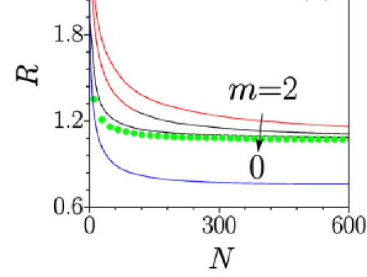
Figure 28: Continuous black and red lines represent dependences of radius $R$ of the coiled axis of the hopfion, along which the wave function vanishes, on its norm, as obtained form the numerical solution of Eq. (6.33). Black and red segments correspond, respectively, to stable and unstable hopfions (the stability boundary splits the solution branch with $s=m=1$ as per Eq. (6.40)). The chain of green dots represents the VA prediction based on ansatz (6.34). The lower blue curve shows the $R(N)$ dependence for a stable hopfion family with $s=1$ and $m=0$, produced by Eq. (6.1) with a smoother spherically isotropic modulation profile, $\sigma(r)=1+r^{6}$, instead of one defined by Eq. (6.14) (source: Kartashov et al., 2014).

As concerns the stability, Fig. 28 demonstrates, as mentioned above, that the hopfions with $s=1,m=0$ are completely stable, the ones with $s=m=1$ are stable at

$$\mu\geq\mu_{\min}\approx 11.2,$$ (231)

and the modes with $s=1,m\geq 2$ are completely unstable.

Finally, the application of torque (6.30), with the axis belonging to the plane of the coiled axis of the hopfion, may readily set the stable hopfion in mechanical rotation around the torque’s axis. An example is displayed in Fig. 29 for the hopfion with $s=1,m=0$.

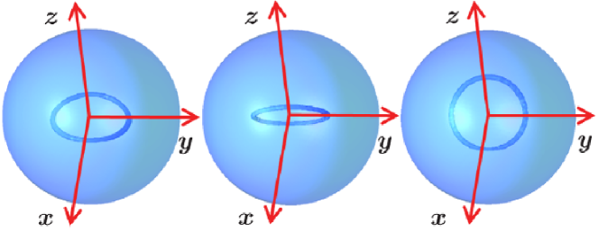
Figure 29: Stable rotation of the hopfion with $s=1,m=0$, initiated by multiplying the stationary wave function by torque factor (6.30) with $\beta=x_{0}=5$. Densities isosurfaces, $\left|\psi\left(x,y,z\right)\right|^{2}=0.2$, are plotted at times $t=141$, $156$, and $177,$ the rotation period being $T\approx 48$ (source: Kartashov et al., 2014).

VI.7 Vortex-antivortex hybrids in the peanut-shaped modulation profile

VI.7.1 Composite modes with opposite vorticities

Another species of unusual 3D self-trapped states is supported by Eq. (6.1) in which the anti-Gaussian isotropic modulation profile (6.14) is replaced by a “peanut”-shaped one, which is stretched along axis $z$ by distance $d$. It was introduced by Driben et al. (1914b) in terms of the cylindrical coordinates:

$$\sigma\left(r,z\right)=\exp\left[\frac{1}{2}\left(r^{2}+\left(|z|-\frac{d}{2}\right)^{2}\right)\right].$$ (232)

If $d$ is large enough, this modulation profile makes it possible to create “hybrid states”, alias composite ones, in the form of vortex tori with opposite winding numbers, $S=\pm 1$, trapped in the top and bottom lobes of the “peanut”. Examples of both the usual vortex mode, with winding numbers $S=1$ in both lobes, i.e., with

$$\psi=e^{iS\theta}w\left(r,z)\right),$$ (233)

and hybrids, with vorticities $\pm 1$ and $\pm 2$, are presented in Fig. 30.

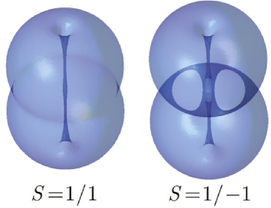
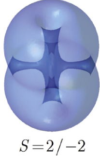
Figure 30: Density profiles of 3D vortex modes supported by Eq. (6.1) with the “peanut”-shaped modulation profile of the local nonlinearity strength, defined as per Eq. (6.41). The profiles are shown by means of isosurfaces $\left|\psi\left(x,y,z\right)\right|^{2}=0.2$. The left panel displays a usual stable vortex state, taken in the form of Eq. (6.42), with equal winding numbers $S=1$ in both lobes of the peanut. The central and right panels represent “hybrids” (composite modes), with opposite vorticities, $S/-S$, in the top and bottom lobes (note the strong breaking of the axial symmetry exhibited by the hybrids). The left and right panels correspond to $d=3$ in Eq. (6.41) and chemical potential $\mu=10$. The central panel corresponds to $d=5$ and $\mu=7$. The usual and hybrid vortex modes with vorticities $1$ and $\pm 1$, shown in the left and central panels, are stable. The hybrid with vorticities $\pm 2$, shown in the right panel, is unstable (source: Driben et al., 2014b).

The hybrid states may be represented by an approximate stationary solution in the following form:

$$\psi=e^{-i\mu t}\left[w_{+}\left(r,z\right)e^{iS\theta}+w_{-}\left(r,z\right)e^{-iS\theta}\right].$$ (234)

The substitution of this ansatz in Eq. (6.1) leads, in the approximation which neglects angular harmonics $\exp\left(\pm 3iS\theta\right)$, to a system of two coupled stationary equations for real functions $w_{\pm}$:

$$\left[\mu+\frac{1}{2}\left(\frac{\partial^{2}}{\partial r^{2}}+\frac{1}{r}\frac{\partial}{\partial r}-\frac{S^{2}}{r^{2}}+\frac{\partial^{2}}{\partial z^{2}}\right)\right]\phi_{\pm}=\sigma\left(r,z\right)\left[2\left(\phi_{\mp}\right)^{2}+\left(\phi_{\pm}\right)^{2}\right]\phi_{\pm},$$ (235)

where $\sigma\left(r,z\right)$ is taken as per Eq. (6.41). Numerical solution of Eqs. (6.44) predicts shapes of the hybrids which are quite close to those produced, as stationary solutions, by full equation (6.1) with the modulation profile (6.41).

The hybrid modes, combining opposite azimuthal harmonics, break the axial symmetry of the resulting states. This can be easily seen looking at ansatz (6.42) in the midplane, $z=0$, where $\phi_{\pm}(r,z=0)$ amount to the single real function, $\phi_{0}(r)$:

$$\left|\psi\left(r,\theta,z=0\right)\right|^{2}=4\phi_{0}^{2}(r)\cos^{2}\left(S\theta\right).$$ (236)

The strong azimuthal pattern exhibited by Eq. (6.45) (it resembles the so-called azimuthon states known in 2D systems (Desyatnikov, Sukhorukov, and Kivshar, 2005)) models the actual structure seen in the middle panel of Fig. 67.

The study of stability of the hybrids was performed by Driben et al. (2014b) by solving the respective BdG equations for small perturbations, and also by means of direct simulations of the perturbed evolution. As a result, it was found that the hybrids with vorticities $\pm 1$ may be stable provided that the stretching parameter $d$ in Eq. (6.41) exceeds a minimum value,

$$d>\left(d_{\min}\right)_{S=+1,-1}\approx 4.$$ (237)

In particular, the hybrids are stable at $\mu<15.8$ (alias $N<394.9$) at $d=4.5$, and at $\mu<13.5$ ($N<329.3$) at $d=5$. The instability of the hybrids at larger values of $\mu$ is explained by the fact that (as shown, in particular, by the TF approximation – see Eq. (6.37)) the increase of $\mu$ makes the localized modes broader, hence the stretching parameter $d$ becomes relatively smaller, failing to produce the stabilization. In direct simulations, those hybrids with $S=\pm 1$ which are unstable develop the instability in the form of corrugation of the mode’s central axis. All hybrids with vorticities $\pm S$ are unstable for $S\geq 2$.

VI.7.2 Fundamental-vortex complexes

The same model, based on Eqs. (6.1) and (6.41), admits dynamical composite modes, in the form of fundamental and vortex states juxtaposed in the bottom and top lobes of the peanut-shaped trapping profile. As shown in Fig. 31, this complex may readily form a state in which the vortex component with $S_{1}=1$ performs completely stable periodic precession on top of the fundamental “base”, with $S_{2}=0$. A broad stability area for the precessing composite states was found provided that $d$ exceeds a minimum value,

$$d>\left(d_{\min}\right)_{S_{1,2}=1,0}\approx 4.8,$$ (238)

cf. Eq. (6.46).

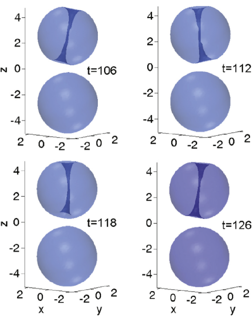
Figure 31: An example of robust periodic precession of a vortex mode with $S=1$ on top of the immobile zero-vorticity one, which are trapped, respectively, in the top and bottom lobes of the “peanut-shaped” structure (6.41) with $d=5$. The initial state was built taking halves of the respective stationary states with $\mu=15$. The motion is displayed by means of density isosurfaces $\left|\psi\left(x,y,z\right)\right|^{2}=1$, produced by simulations of Eq. (6.1). In the present case, the period of the precession is $\approx 20$ (source: Driben et al., 2014b).

VI.8 Weakly localized dark vortices

As mentioned above, the fundamental condition which secures the convergence of the norm of localized modes produced by Eqs. (6.1) and (6.6) is given by Eq. (6.8). If this condition does not hold, Eq. (6) gives rise to weakly localized states with the divergent norm, which may be considered as localized dark solitons (Zeng and Malomed, 2017), as they share the property of the divergence of the norm with dark solitons in usual (free-space) models.

Localized dark solitons were considered by Zeng and Malomed (2017) in the 2D version of Eq. (6.1) with the modulation profile

$$\sigma(r)=r^{\alpha},~{}\alpha\leq 2,$$ (239)

cf. Eq. (6.10). The weakly localized solutions to Eq. (6.1) with vorticity $S$ were looked for, in the polar coordinates, as

$$\psi=\exp\left(-i\mu t+iS\theta\right)w(r),$$ (240)

(essentially the same as Eq. (6.11)), where real function $w(r)$ satisfies the equation

$$\mu w+\frac{1}{2}\left(\frac{d^{2}w}{dr^{2}}+\frac{1}{r}\frac{dw}{dr}-\frac{S^{2}}{r^{2}}w\right)-r^{\alpha}w^{3}=0,$$ (241)

cf. Eq. (6.12). The asymptotic form of the solution at $r\rightarrow\infty$ is

$$w=\sqrt{\mu}r^{-\alpha/2}+\frac{1}{4\sqrt{\mu}}\left(\frac{\alpha^{2}}{4}-S^{2}\right)r^{-\alpha/2-2}+\mathcal{O}\left(r^{-\alpha/2-4}\right),$$ (242)

where the first term is tantamount to the TF approximation, cf. Eq. (6.9). Solutions (6.49) with $S=0$ and $S\neq 0$ may be called, respectively, localized CW states and localized dark vortices.

First, in the case of $\alpha=2$, which corresponds to the boundary between localized dark and bright states, Eq. (6.50) with $S=1$ gives rise to simple exact solutions, for all values $\mu>0$ (although these dark-vortex solutions are unstable, see Fig. 33 below):

$$w(r;\alpha=2;S=1)=\sqrt{\mu}r^{-1}.$$ (243)

Obviously, the divergence of the integral norm of solutions to Eq. (6.50) is logarithmic at $r\rightarrow\infty$.

The dark CW states may be quite accurately approximated by the TF approximation (which corresponds to the first term on the right-hand side of Eq. (6.51)) multiplied by a factor which accounts for vorticity $S\geq 1$:

$$w(r)=\sqrt{\mu}r^{-\alpha/2}\left[\tanh(\lambda r)\right]^{S},$$ (244)

where $\lambda$ is a fitting parameter. Typical radial profiles of the localized dark vortices, along with approximation (6.53), are displayed, for $S=1$ and $2$, in Fig. 32.

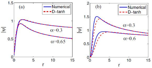
Figure 32: Blue lines show examples of localized dark vortices, produced by the numerical solution of Eq. (6.50) with values of $\alpha$ indicated in the figure, and vorticities $S=1$ (a) and $S=2$ (b). The chemical potential is $\mu=4$ for $\alpha=0.6$ in (b), and $\mu=1.5$ for other solutions. Red dashed lines show the analytical approximation given by Eq. (6.53), with fitting factors $\lambda=1.1$ in (a), and $\lambda=1.5$ in (b). The vortices with $S=1$ shown in (a) are stable, while the double vortices in (b) are weakly unstable (source: Zeng and Malomed, 2017).

Stability of the localized CW states and dark vortices was identified by means of systematic simulations of their perturbed evolution in the framework of the Eq. (6.1). The conclusion is that the CW states are completely stable (actually, they realize the system’s ground state), while all the localized dark vortices with $S\geq 2$ are unstable. The analysis for vortices with $S=1$ produces a nontrivial stability boundary, which is shown in Fig. 33. It shows that the increase of both $\mu$ and $\alpha$ leads to destabilization of the dark vortex. Actually, they may be stable only at

$$\alpha<\alpha_{\max}\approx 0.55,$$ (245)

i.e., if the the dark vortex is sufficiently stretched in the radial direction (as seen from the approximate expression (6.53)).

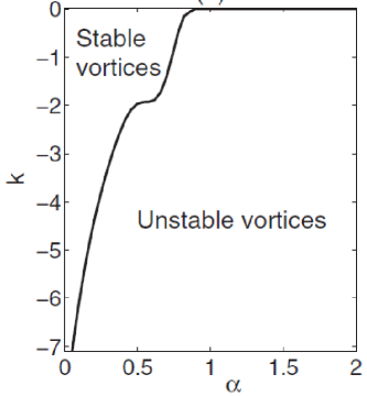
Figure 33: The stability chart for the localized dark vortices with $S=1$, produced by Eq. (6.50). In this plot, notation $k\equiv-\mu$ is used. The vortices are completely unstable at $\alpha>0.55,$ see Eq. (6.54). All the localized dark states with $S=0$ (CW) are completely stable, while all vortices with $S\geq 2$ are unstable (source: Zeng and Malomed, 2017).

VII Conclusion

This chapter produces a systematic summary of theoretical results, both numerical and analytical ones, obtained in numerous works aimed at the search for physically relevant settings which allow one to create stable 2D and 3D solitons, including topological modes with embedded vorticity, as well as complex 3D modes in the form of hopfions, which carry two independent topological charges. Stability is the main challenge in the studies of multidimensional solitons because, on the contrary to diverse 1D settings, in which solitons typically emerge as stable objects, they tend to be strongly unstable in basic 2D and 3D situations. In particular, the ubiquitous NLS (nonlinear Schrödinger) equation with the cubic self-focusing term (essentially the same PDE is known as the GP (Gross-Pitaevskii) equation in the BEC theory) creates only unstable solitons in 2D and 3D spaces alike, because exactly the same equation gives rise to the destructive effects in the form of the critical and supercritical wave collapse in 2D and 3D cases, respectively.

The present chapter is focused on physically relevant multidimensional models of the NLS/GP type. The chapter offers a relatively detailed review of two  basic topics. First, it is a general survey of various schemes which have been elaborated to secure stability of 2D and 3D solitons, including those with embedded vorticity. The main stabilization schemes outlined here are: (i) competing (e.g., cubic-quintic) and saturable nonlinearities; (2) linear and nonlinear trapping potentials; (3) the stabilizing effect provided by the LHY (Lee-Huang-Yang) corrections to the mean-field BEC dynamics, leading to the formation of stable QDs (quantum droplets), including ones with embedded vorticity; (4) SOC (spin-orbit-coupling) effects in two- and three-dimensional binary BEC; and (5) emulation of SOC in nonlinear optical waveguides, including $\mathcal{PT}$-symmetric ones.

The second topic addressed in the chapter is a detailed summary of results which demonstrate the creation of stable 2D and 3D solitons by means of schemes based on the usual linear trapping potentials or effective nonlinear ones. Nonlinear potentials may be induced by means of spatial modulation of the local strength of the nonlinear term. The latter option is especially promising, making it possible to use self-defocusing media, with the local nonlinearity strength growing fast enough from the center to periphery, for the creation of a great variety of multidimensional self-trapped modes. In addition to fundamental quasi-solitons and vortex rings, the 3D modes may be hopfions, i.e., twisted vortex rings. A remarkable fact is that many essential results for the multidimensional solitons can be obtained, in such settings, not only in a numerical form, but also by means of efficient analytical methods, exact and approximate ones. In particular, basic properties of such complex objects as hopfions are accurately predicted by the analytical variational approximation.

The work on the vast topic surveyed in this chapter is far from being completed. Among challenging open problems is, for instance, a possibility to create stable complex 3D structures in the form of two linked rings, each one being a vortex torus or, possibly, a hopfion. The greatest challenge is to implement many theoretical predictions, outlined in the present review, in real physical experiments – especially in BEC and nonlinear optics.

References

- [1] Abdullaev F. Kh. and M. Salerno, “Gap-Townes solitons and localized excitations in low-dimensional Bose-Einstein condensates in optical lattices”, Phys. Rev. A 72, 033617 (2005).
- [2] Ablowitz M. and H. Segur, Solitons and the Inverse Scattering Transform (SIAM, Philadelphia, 1981).
- [3] Adhikari S. K., “Collapse of attractive Bose-Einstein condensed vortex states in a cylindrical trap”, Phys. Rev. E 65, 016703 (2001).
- [4] Adhikari S. K., Multiring, stripe, and superlattice solitons in a spin-orbit-coupled spin-1 condensate, Phys. Rev. A 103, L011301 (2021).
- [5] Alexander T. J. and L. Bergé, “Ground states and vortices of matter-wave condensates and optical guided waves”, Phys. Rev. E 65, 026611 (2002).
- [6] Anderson D., and M. Bonnedal, “Variational approach to nonlinear self-focusing of Gaussian laser beams”, Phys. Fluids 22, 105-109 (1979)
- [7] Anderson D., “Variational approach to nonlinear pulse propagation in optical fibers”, Phys. Rev. A 27, 3135-3144 (1983).
- [8] Baizakov B. B., B. A. Malomed, and M. Salerno, “Multidimensional solitons in periodic potentials”. Europhys. Lett. 63, 642-648 (2003).
- [9] Baizakov B. B., B. A. Malomed, and M. Salerno, “Multidimensional solitons in a low-dimensional periodic potential”, Phys. Rev. A 70, 053613 (2004).
- [10] Baizakov B. B., B. A. Malomed, and M. Salerno, “Matter-wave solitons in radially periodic potentials”, Phys. Rev. E 74, 066615 (2006).
- [11] Bakkali-Hassani B., C. Maury, Y.-Q. Zou, E. Le Cerf, R. Saint-Jalm, P. C. M. Castilho, S. Nascimbene, J. Dalibard, and J. Beugnon, “Realization of a Townes Soliton in a Two-Component Planar Bose Gas”, Phys. Rev. Lett. 127, 023603 (2021).
- [12] Bao W. Z. and Y. Y. Cai, ”Mathematical theory and numerical methods for Bose-Einstein condensation”, Kinetic and Related Models 6, 1-135 (2013).
- [13] Bao W. Z. and Q. Du, “Computing the ground state solution of Bose-Einstein condensates by a normalized gradient flow”, SIAM J. Sci. Comp. 25, 1674-1697 (2004).
- [14] Bao W. Z., D. Jaksch, and P. A. Markowich, “Numerical solution of the Gross-Pitaevskii equation for Bose-Einstein condensation”, J. Comp. Phys. 187, 318-342 (2003).
- [15] Bauer D. M., M. Lettner, C. Vo, G. Rempe, and S. Dürr, “Control of a magnetic Feshbach resonance with laser light”, Nature Phys. 5, 339-342 (2009)
- [16] Bender C. M., “Making sense of non-Hermitian Hamiltonians”, Rep. Prog. Phys. 70, 947-1018 (2007).
- [17] Bergé L., “Wave collapse in physics: principles and applications to light and plasma waves”, Phys. Rep. 303, 259-370 (1998).
- [18] Borovkova O. V., Y. V. Kartashov, B. A. Malomed, and L. Torner, Algebraic bright and vortex solitons in defocusing media, Opt. Lett. 36, 3088-3090 (2011a).
- [19] Borovkova O. V., Y. V. Kartashov, L. Torner, and B. A. Malomed, Bright solitons from defocusing nonlinearities, Phys. Rev. E 84, 035602 (R) (2011b).
- [20] G. Boudebs, S. Cherukulappurath, H. Leblond, J. Troles, F. Smektala, and F. Sanchez, “Experimental and theoretical study of higher-order nonlinearities in chalcogenide glasses”, Opt. Commun. 219, 427-432 (2003).
- [21] Bradley C. C., C. A. Sackett, J. J. Tollett, and R. G. Hulet, “Evidence of Bose-Einstein condensation in an atomic gas with attractive interactions”, Phys. Rev. Lett. 75, 1687-1690 (1995); Erratum: Phys. Rev. Lett. 79, 1170 (1997).
- [22] Brazhnyi V. A. and V. V. Konotop, Theory of nonlinear matter waves in optical lattices, Mod. Phys. Lett. B 18, 627-651 (2004).
- [23] Brtka M., A. Gammal, and B. A. Malomed, “Hidden vorticity in binary Bose-Einstein condensates”, Phys. Rev. A 82, 053610 (2010).
- [24] Burlak G. and B. A. Malomed, “Stability boundary and collisions of two-dimensional solitons in -symmetric couplers with the cubic-quintic nonlinearity”, Phys. Rev. E 88, 062904 (2013).
- [25] Buryak A. V., P. Di Trapani, D. V. Skryabin, and S. Trillo, “Optical solitons due to quadratic nonlinearities: from basic physics to futuristic applications”, Phys. Rep. 370, 63-235 (2002).
- [26] Bychkov Yu. A. and E. I. Rashba, “Oscillatory effects and the magnetic susceptibility of carriers in inversion layers”, J. Phys. C: Solid State Phys. 17, 6039-6045 (1984).
- [27] Cabrera C., L. Tanzi, J. Sanz, B. Naylor, P. Thomas, P. Cheiney, and L. Tarruell, “Quantum liquid droplets in a mixture of Bose-Einstein condensates”, Science 359, 301-304 (2018).
- [28] Calogero F, and A. Degasperis, Spectral Transform and Solitons: Tools to Solve and Investigate Nonlinear Evolution Equations (North-Holland, Amsterdam, 1982).
- [29] Carr L. D. and C. W. Clark, “Vortices in attractive Bose-Einstein condensates in two dimensions”, Phys. Rev. Lett. 97, 010403 (2006).
- [30] Cheiney P., C. R. Cabrera, J. Sanz, B. Naylor, L. Tanzi, and L. Tarruell, “Bright soliton to quantum droplet transition in a mixture of Bose-Einstein condensates”, Phys. Rev. Lett. 120, 135301 (2018).
- [31] Chen C.-A. and C.-L. Hung, “Observation of Universal Quench Dynamics and Townes Soliton Formation from Modulational Instability in Two-Dimensional Bose Gases”, Phys. Rev. Lett. 125, 250401 (2020).
- [32] Chen C.-A. and C.-L. Hung, “Observation of scale invariance in two-dimensional matter-wave Townes solitons”, Phys. Rev. Lett. 127, 023604 (2021).
- [33] Chen H.-H. and C.-H. Liu, “Solitons in nonuniform media”, Phys. Rev. Lett. 37, 693-697 (1976).
- [34] Chiao R. Y., E. Garmire, and C. H. Townes, “Self-trapping of optical beams”, Phys. Rev. Lett. 13, 479-482 (1964).
- [35] Chin C., R. Grimm, P. Julienne, and E. Tiesinga, “Feshbach resonances in ultracold gases”, Rev. Mod. Phys. 82, 1225-1286 (2010).
- [36] Clark L. W., L.-C. Ha, C.-Y. Xu, and C. Chin, “Quantum dynamics with spatiotemporal control of interactions in a stable Bose-Einstein condensate”, Phys. Rev. Lett. 115, 155301 (2015).
- [37] Coutaz J. L. and M. Kull, “Saturation of the nonlinear index of refraction in semiconductor-doped glass”, J. Opt. Soc. Am. B 8, 95-98 (1991).
- [38] Dauxois T. and M. Peyrard, Physics of Solitons (Cambridge University Press, Cambridge, 2006), ISBN 0-521-85421-0.
- [39] Davydova T. A. and A. I. Yakimenko, “Stable multicharged localized optical vortices in cubic–quintic nonlinear media”, J. Optics A: Pure Appl. Opt. 6, S197-S201 (2004).
- [40] D’Errico, C., A. Burchianti, M. Prevedelli, L. Salasnich, F. Ancilotto, M. Modugno, F. Minardi, and C. Fort, “Observation of quantum droplets in a heteronuclear bosonic mixture”, Phys. Rev. Res. 1, 033155 (2019).
- [41] Desaix M., D. Anderson, and M. Lisak, “Variational approach to collapse of optical pulses”, J. Opt. Soc. Am. B 8, 2082-2086 (1991).
- [42] Desyatnikov, A. S., A. A. Sukhorukov, and Y. S. Kivshar, “Azimuthons: Spatially modulated vortex solitons”, Phys. Rev. Lett. 95, 203904 (2005).
- [43] Dolgaleva K., H. Shin, and R. W. Boyd, “Observation of a microscopic cascaded contribution to the fifth-order nonlinear susceptibility”, Phys. Rev. Lett. 103, 113902 (2009).
- [44] Dresselhaus G., “Spin-orbit coupling effects in zinc blende structures”, Phys. Rev. 100, 580-586 (1955).
- [45] Driben R. and B. A. Malomed, “Stability of solitons in parity-time-symmetric couplers”, Opt. Lett. 36, 4323-4325 (2011).
- [46] Driben R., Y. V. Kartashov, B. A. Malomed, T. Meier, and L. Torner, “Soliton gyroscopes in media with spatially growing repulsive nonlinearity”, Phys. Rev. Lett. 112, 020404 (2014a).
- [47] Driben R., Y. Kartashov, B. A. Malomed, T. Meier, and L. Torner, “Three-dimensional hybrid vortex solitons”, New J. Phys. 16, 063035 (2014b).
- [48] Dror N. and B. A. Malomed, “Symmetric and asymmetric solitons and vortices in linearly coupled two-dimensional waveguides with the cubic-quintic nonlinearity”, Physica D 240, 526-541 (2011).
- [49] Duncan D. B., J. C. Eilbeck, H. Feddersen, and J. A. D. Wattis, “Solitons on lattices”, Physica D 68, 1-11 (1993).
- [50] Dutta O., M. Gajda, P. Hauke, M. Lewenstein, D.-S. Luhmann, B. Malomed, T. Sowinski, and J. Zakrzewski, “Non-standard Hubbard models in optical lattices: a review”, Rep. Prog. Phys. 78, 066001 (2015).
- [51] Edilson L., L. Falcão Filho, C. B. de Araújo, G. Boudebs, H. Leblond, and V. Skarka, “Robust two-dimensional spatial solitons in liquid carbon disulfide”, Phys. Rev. Lett. 110, 013901 (2013).
- [52] Efremidis, N. K., J. Hudock, D. N. Christodoulides, J. W. Fleischer, O. Cohen, and M. Segev “Two-dimensional optical lattice solitons,” Phys. Rev. Lett. 91, 213905 (2003).
- [53] Efremidis N. K., Sears S., Christodoulides D. N., Fleischer J. W., and M. Segev, “Discrete solitons in photorefractive optically induced photonic lattices”, Phys. Rev. E 66, 046602 (2002).
- [54] Faddeev L. D., “Some comments on the many-dimensional solitons”, Lett. Math. Phys. 1, 289-293 (1976).
- [55] Faddeev L. D and Niemi A. J., “Knots and particles”, Nature 387, 58-61 (1997).
- [56] Fetter A. L., “Rotating trapped Bose-Einstein condensates”, Rev. Mod. Phys. 81, 657-691 (2009).
- [57] Fibich G., The Nonlinear Schrödinger Equation: Singular Solutions and Optical Collapse (Springer, Heidelberg, 2015).
- [58] Firth W. J. and D. V. Skryabin, “Optical solitons carrying orbital angular momentum”, Phys. Rev. Lett. 79, 2450-2453 (1997).
- [59] Freilich D. V., D. M. Bianchi, A. M. Kaufman, T. K. Langin, and D. S. Hall, “Real-time dynamics of single vortex lines and vortex dipoles in a Bose-Einstein condensate”, Science 329, 1182-1185 (2010).
- [60] Galitski V. and I. B. Spielman, “Spin-orbit coupling in quantum gases”, Nature 494, 49-54 (2013).
- [61] Gaunt A. L., T. F. Schmidutz, I. Gotlibovych, R. P. Smith, and Z. Hadzibabic, “Bose-Einstein condensation of atoms in a uniform potential”, Phys. Rev. Lett. 110, 200406 (2013).
- [62] Gautam S. and S. K. Adhikari, “Three-dimensional vortex-bright solitons in a spin-orbit-coupled spin-1 condensate”, Phys. Rev. A 97, 013629 (2018).
- [63] Ghanbari, S., T. D. Kieu, A. Sidorov, and P. Hannaford, “Permanent magnetic lattices for ultracold atoms and quantum degenerate gases,” J. Phys. B: At. Mol. Opt. Phys. 39, 847-860 (2006).
- [64] Greenberg J. A. and D. J. Gauthier, “High-order optical nonlinearity at low light levels”, EPL 98, 24001 (2012).
- [65] Harrison, W. A., Pseudopotentials in the Theory of Metals (Benjamin, New York, 1966).
- [66] Hauke P., F. M. Cucchietti, L. Tagliacozzo, I. Deutsch, and M. Lewenstein, “Can one trust quantum simulators?”, Rep. Prog. Phys. 75, 082401 (2012).
- [67] Hu H. and X.-J. Liu, “Microscopic derivation of the extended Gross-Pitaevskii equation for quantum droplets in binary Bose mixtures”, Phys. Rev. A 102, 043302 (2020).
- [68] Hueck K., N. Luick, L. Sobirey, J. Siegl, T. Lompe, and H. Moritz, “Two-dimensional homogeneous Fermi gases”, Phys. Rev. Lett. 120, 060402 (2018).
- [69] Hukriede, J., D. Runde, and D. Kip, “Fabrication and application of holographic Bragg gratings in lithium niobate channel waveguides,” J. Phys. D 36, R1 (2003).
- [70] Ilg T., J. Kumlin, L. Santos, and D. S. Petrov, and, H. P. Büchler, “Dimensional crossover for the beyond-mean-field correction in Bose gases”, Phys. Rev. A 98, 051604 (2018).
- [71] Joannopoulos J. D., S. G. Johnson, J. N. Winn, and R. D. Meade, Photonic Crystals: Molding the Flow of Light (Princeton University Press, Princeton, 2008).
- [72] Kartashov Y. V., B. A. Malomed, and L. Torner, “Solitons in nonlinear lattices”, Rev. Mod. Phys. 83, 247-306 (2011).
- [73] Kartashov Y. V., V. A. Vysloukh, L. Torner, and B. A. Malomed, “Self-trapping and splitting of bright vector solitons under inhomogeneous defocusing nonlinearities”, Opt. Lett. 36, 4587-4589 (2011).
- [74] Kartashov Y. V., B. A. Malomed, Y. Shnir, and L. Torner, “Twisted toroidal vortex-solitons in inhomogeneous media with repulsive nonlinearity”, Phys. Rev. Lett. 113, 264101 (2014).
- [75] Kartashov Y. V., B. A. Malomed, V. V. Konotop, V. E. Lobanov, and L. Torner, “Stabilization of solitons in bulk Kerr media by dispersive coupling”, Opt. Lett. 40, 1045-1048 (2015).
- [76] Kartashov Y. V., B. A. Malomed, V. A. Vysloukh, M. R. Belić, and L. Torner, Rotating vortex clusters in media with inhomogeneous defocusing nonlinearity, Opt. Lett. 42, 446-449 (2017).
- [77] Kartashov Y. V., B. A. Malomed, L. Tarruell, and L. Torner, “Three-dimensional droplets of swirling superfluids”, Phys. Rev. A 98, 013612 (2018).
- [78] Kartashov Y., G. Astrakharchik, B. Malomed, and L. Torner, “Frontiers in multidimensional self-trapping of nonlinear fields and matter”, Nature Reviews Phys. 1, 185-197 (2019)
- [79] Kartashov Y. V., L. Torner, M. Modugno, E. Ya. Sherman, B. A. Malomed, and V. V. Konotop, “Multidimensional hybrid Bose-Einstein condensates stabilized by lower-dimensional spin-orbit coupling”, Phys. Rev. Research 2, 013036 (2020).
- [80] Kivshar Y. S and G. P. Agrawal, Optical Solitons: From Fibers to Photonic Crystals (Academic Press, San Diego, 2003).
- [81] Kong D. G., Q. Chang, H. A. Ye, Y. C. Gao, Y. X. Wang, X. R. Zhang, K. Yang, W. Z. Wu, and Y. L. Song, “The fifth-order nonlinearity of CS2”, J. Phys. B: At. Mol. Opt. Phys. 42, 065401 (2009).
- [82] Konotop V. V., J. Yang, and D. A. Zezyulin, “Nonlinear waves in -symmetric systems”, Rev. Mod. Phys. 88, 035002 (2016).
- [83] Kruglov V. I. and R. A. Vlasov, “Spiral self-trapping propagation of optical beams”, Phys. Lett. A 111, 401-404 (1985).
- [84] Kruglov V. I., V. M. Volkov, R. A. Vlasov, and V. V. Drits, “Auto-waveguide propagation and the collapse of spiral light beams in non-linear media,” J. Phys. A: Math. Gen. 21, 4381–4395 (1988).
- [85] Lavoine L. and T. Bourdel, Beyond-mean-field crossover from one dimension to three dimensions in quantum droplets of binary mixtures, Phys. Rev. A 103, 033312 (2021).
- [86] Leblond H., B. A. Malomed, and D. Mihalache, “Three-dimensional vortex solitons in quasi-two-dimensional lattices”, Phys. Rev. E 76, 026604 (2007).
- [87] Lederer F., G. I. Stegeman, D. N. Christodoulides, G. Assanto, M. Segev, and Y. Silberberg, “Discrete solitons in optics”, Phys. Rep. 463, 1-126 (2008).
- [88] Lee T. D., K. Huang, and C. N. Yang, “Eigenvalues and eigenfunctions of a Bose system of hard spheres and its low-temperature properties”, Phys. Rev. 106, 1135-1145 (1957).
- [89] Lewenstein M., A. Sanpera, and V. Ahufinger, Ultracold Atoms in Optical Lattices: Simulating Quantum Many-Body Systems (Oxford: Oxford University Press, 2012)
- [90] Li Y., Y. Liu, Z. Fan, W. Pang, S. Fu, and B. A. Malomed, “Two-dimensional dipolar gap solitons in free space with spin-orbit coupling”, Phys. Rev. A 95, 063613 (2017).
- [91] Li Y., Z. Chen, Z. Luo, C. Huang, H. Tan, W. Pang, and B. A. Malomed, Two-dimensional vortex quantum droplets, Phys. Rev. A 98, 063602 (2018).
- [92] Liberal I. and N. Engheta, “Near-zero refractive index photonics,” Nature Photonics 11, 149-158 (2017).
- [93] Lin Y.-J., K. Jiménez-García, and I. B. Spielman, “Spin-orbit-coupled Bose-Einstein condensates”, Nature 471, 83-86 (2011).
- [94] Luo D., Y. Jin, J. H. V. Nguyen, B. A. Malomed, O. V. Marchukov, V. A. Yurovsky, V. Dunjko, M. Olshanii, and R. G. Hulet, “Creation and characterization of matter-wave breathers”, Phys. Rev. Lett. 125, 183902 (2020).
- [95] Makris, K. G., R. El-Ganainy, D. N. Christodoulides, and Z. H. Musslimani, “ symmetric periodic optical potentials”, Int. J. Theor. Phys. 50, 1019-1041 (2011).
- [96] Malomed B. A., “Variational methods in nonlinear fiber optics and related fields”, Prog. Optics 43, 71-193 (2002); http://www.sciencedirect.com/science/article/pii/S0079663802800269.
- [97] Malomed B. A., “Multidimensional solitons: Well-established results and novel findings”, Eur. Phys. J. Special Topics 225, 2507-2532 (2016).
- [98] Malomed B. A., (INVITED) Vortex solitons: Old results and new perspectives, Physica D 399, 108-137 (2019).
- [99] Malomed B. A., L.-C. Crasovan, and D. Mihalache, “Stability of vortex solitons in the cubic-quintic model”, Physica D 161, 187-201 (2002).
- [100] Malomed, B. A., F. Lederer, D. Mazilu, and D. Mihalache, “On stability of vortices in three-dimensional self-attractive Bose-Einstein condensates”, Phys. Lett. A 361, 336-340 (2007).
- [101] Malomed B. A., D. Mihalache, F. Wise, and L. Torner, “Spatiotemporal optical solitons”, J. Optics B: Quant. Semicl. Opt. 7, R53-R72 (2005).
- [102] Malomed B. A., D. Mihalache, F. Wise, and L. Torner, “Viewpoint: On multidimensional solitons and their legacy in contemporary Atomic, Molecular and Optical physics”, J. Phys. B: At. Mol. Opt. Phys. 49, 170502 (2016).
- [103] Malomed B. A. and D. E. Pelinovsky, “Persistence of the Thomas-Fermi approximation for ground states of the Gross-Pitaevskii equation supported by the nonlinear confinement”, Appl. Math. Lett. 40, 45-48 (2015).
- [104] Manton N. and P. Sutcliffe, Topological Solitons (Cambridge University Press, Cambridge, 2004).
- [105] Mihalache D., D. Mazilu, L.-C. Crasovan, B. A. Malomed, F. Lederer, and L. Torner, “Soliton clusters in three-dimensional media with competing cubic and quintic nonlinearities”, J. Optics B 6, S333-S340 (2004a).
- [106] Mihalache, D. D. Mazilu, F. Lederer, Y. V. Kartashov, L.-C. Crasovan, and L. Torner, “Stable three-dimensional spatiotemporal solitons in a two-dimensional photonic lattice”, Phys. Rev. E 70, 055603(R) (2004b).
- [107] Mihalache D., D. Mazilu, B. A. Malomed, and F. Lederer. Vortex stability in nearly-two-dimensional Bose-Einstein condensates with attraction. Phys. Rev. A 73, 043615 (2006).
- [108] Mihalache D., “Multidimensional localized structures in optical and matter-wave media: A topical survey of recent literature”, Romanian Reports in Physics 69, 403 (2017).
- [109] Mineev V. P., “The theory of the solution of two near-ideal Bose gases”, Zh. Eksp. Teor. Fiz. 67, 263-272 (1974) [English translation: Sov. Phys. – JETP 40, 132-136 (1974)].
- [110] Moiseyev N., Non-Hermitian Quantum Mechanics (Cambridge University Press, Cambridge, 2011).
- [111] O. Morsch and M. Oberthaler, “Dynamics of Bose-Einstein condensates in optical lattices”, Rev. Mod. Phys. 78, 179-212 (2006).
- [112] Möttönen M., S. M. M. Virtanen, T. Isoshima, and M. M. Salomaa, “Stationary vortex clusters in nonrotating Bose-Einstein condensates”, Phys. Rev. A 71, 033626 (2005).
- [113] Muruganandam P. and S. K. Adhikari, “Fortran programs for the time-dependent Gross-Pitaevskii equation in a fully anisotropic trap”, Comp. Phys. Comm. 180, 1888-1912 (2009).
- [114] Navon N., A. L. Gaunt, R. P. Smith, and Z. Hadzibabic, “Critical dynamics of spontaneous symmetry breaking in a homogeneous Bose gas”, Science 347, 167-170 (2015).
- [115] Newell A., Solitons in Mathematics and Physics (SIAM, Philadelphia, 1985).
- [116] Niu X., X. Hu, S. Chu, and Q. Gong, “Epsilon-near-zero photonics: a new platform for integrated devices,” Adv. Opt. Mater. 6, 1701292 (2018).
- [117] Pego R. L. and H. A. Warchall, “Spectrally stable encapsulated vortices for nonlinear Schrödinger equations, J. Nonlinear Sci. 12, 347-394 (2002).
- [118] Petrov D. S., “Quantum mechanical stabilization of a collapsing Bose-Bose mixture. Phys. Rev. Lett. 115, 155302 (2015).
- [119] Petrov D. S. and G. E. Astrakharchik, “Ultradilute low-dimensional liquids”, Phys. Rev. Lett. 117, 100401 (2016).
- [120] Pitaevskii L. P. and S. Stringari, Bose-Einstein Condensation (Oxford University Press, Oxford, 2003).
- [121] Pollack S. E., D. Dries, M. Junker, Y. P. Chen, T. A. Corcovilos, and R. G. Hulet, Extreme Tunability of Interactions in a Li-7 Bose-Einstein Condensate, Phys. Rev. Lett. 102, 090402 (2009).
- [122] Qin J., G. Dong, and B. A. Malomed, “Stable giant vortex annuli in microwave-coupled atomic condensates,” Phys. Rev. A 94, 053611 (2016).
- [123] Quiroga-Teixeiro M. and H. Michinel, “Stable azimuthal stationary state in quintic nonlinear optical media”, J. Opt. Soc. Amer. B 14, 2004-2009 (1997).
- [124] Reshef O., E. Giese, M. Z. Alam, I. de Leon, J. Upham, and R. W. Boyd, “Beyond the perturbative description of the nonlinear optical response of low-index materials”, Opt. Lett. 42, 3225-3228 (2017).
- [125] Reyna A. S. and C. B. de Araújo, “Spatial phase modulation due to quintic and septic nonlinearities in metal colloids”, Opt. Exp. 22, 22456 (2014).
- [126] Reyna A. S., G. Boudebs, B. A. Malomed, and C. B. de Araújo, “Robust self-trapping of vortex beams in a saturable optical medium”, Phys. Rev. A 93, 013840 (2016).
- [127] Rogers C. and W. K. Schief, Bäcklund and Darboux Transformations: Geometry and Modern Applications in Soliton Theory (Cambridge University Press, New York, 2002).
- [128] Saito H. and M. Ueda, “Split instability of a vortex in an attractive Bose-Einstein condensate”, Phys. Rev. Lett. 89, 190402 (2002).
- [129] Sakaguchi H., B. Li, and B. A. Malomed, “Creation of two-dimensional composite solitons in spin-orbit-coupled self-attractive Bose-Einstein condensates in free space”, Phys. Rev. E 89, 032920 (2014).
- [130] Sakaguchi H. and B. A. Malomed, “Two-dimensional loosely and tightly bound solitons in optical lattices and inverted traps”, J. Phys. B 37, 2225-2239 (2004).
- [131] Sakaguchi H. and B. A. Malomed, Two-dimensional solitons in the Gross-Pitaevskii equation with spatially modulated nonlinearity, Phys. Rev. E 73, 026601 (2006).
- [132] Sakaguchi H. and B. A. Malomed, “Solitons in combined linear and nonlinear lattice potentials”, Phys. Rev. A 81, 013624 (2010).
- [133] Sakaguchi H. and B. A. Malomed, Suppression of the quantum-mechanical collapse by repulsive interactions in a quantum gas, Phys. Rev. A 83, 013607 (2011).
- [134] Sakaguchi H. and B. A. Malomed, “Stable two-dimensional solitons supported by radially inhomogeneous self-focusing nonlinearity”, Opt. Lett. 37, 1035-1037 (2012).
- [135] Sakaguchi H. and B. A. Malomed, “One- and two-dimensional solitons in -symmetric systems emulating spin-orbit coupling”, New J. Phys. 18, 105005 (2016).
- [136] Sakaguchi H. and B. A, Malomed, One- and two-dimensional gap solitons in spin-orbit-coupled systems with Zeeman splitting, Phys. Rev. A 97, 013607 (2018).
- [137] Sakaguchi H., B. Li, E. Ya. Sherman, and B. A. Malomed, “Composite solitons in two-dimensional spin-orbit coupled self-attractive Bose-Einstein condensates in free space”, Romanian Reports in Physics 70, 502 (2018).
- [138] Salasnich L., B. A. Malomed, and F. Toigo, “Matter-wave vortices in cigar-shaped and toroidal waveguides”, Phys. Rev. A 76, 063614 (2007).
- [139] Satsuma J. and N. Yajima, “Initial Value Problems of One-Dimensional Self-Modulation of Nonlinear Waves in Dispersive Media”, Suppl. Prog. Theor. Phys. No. 55, 284-306 (1974).
- [140] Segev M., B. Crosignani, A. Yariv, and B. Fischer, “Spatial solitons in photorefractive media”, Phys. Rev. Lett. 68, 923-926 (1992).
- [141] Semeghini G., G. Ferioli, L. Masi, C. Mazzinghi, L. Wolswijk, F. Minardi, M. Modugno, G. Modugno, M. Inguscio, and M. Fattori, “Self-bound quantum droplets of atomic mixtures in free space?”, Phys. Rev. Lett. 120, 235301 (2018).
- [142] Shamriz E., Z. Chen, and B. A. Malomed, Suppression of the quasi-two-dimensional quantum collapse in the attraction field by the Lee-Huang-Yang effect, Phys. Rev. A 101, 063628 (2020a).
- [143] Shamriz E., Z. Chen, and B. A. Malomed, “Stabilization of one-dimensional Townes solitons by spin-orbit coupling in a dual-core system”, Comm. Nonlin. Sci. Numer. Simul. 91, 105412 (2020b).
- [144] Silberberg Y., “Collapse of optical pulses,” Opt. Lett. 15, 1282-1284 (1990).
- [145] M. Skorobogatiy M. and J. Yang, Fundamentals of Photonic Crystal Guiding (Cambridge University Press, Cambridge, 2009).
- [146] P. M. Sutcliffe, “Knots in the Skyrme–Faddeev model”, Proc. R. Soc. A 463, 3001-3020 (2007).
- [147] Takhtadjian L. A. and L. D. Faddeev, The Hamiltonian Approach in the Theory of Solitons (Nauka Publishers, Moscow, 1986).
- [148] Tian Q., L. Wu, Y. Zhang, and J.-F. Zhang, “Vortex solitons in defocusing media with spatially inhomogeneous nonlinearity”, Phys. Rev. E 85, 056603 (2012).
- [149] Tojo S., Y. Taguchi, Y. Masuyama, T. Hayashi, H. Saito, and T. Hirano, “Controlling phase separation of binary Bose-Einstein condensates via mixed-spin-channel Feshbach resonance”, Phys. Rev. A 82, 033609 (2010).
- [150] Tominaga K. and K. Yoshihara, Fifth order optical response of liquid CS2 observed by ultrafast nonresonant six-wave mixing, Phys. Rev. Lett. 74, 3061 (1995).
- [151] Vakhitov N. G. and A. A. Kolokolov, “Stationary solutions of the wave equation in a medium with nonlinearity saturation”, Radiophys. Quantum Electron. 16, 783-789 (1973); https://doi.org/10.1007/BF01031343.
- [152] Vlasov S. N., V. A. Petrishchev, and V. I. Talanov, Izv. Vyssh. Uchebn. Zaved. Radiofiz. 14, 1353 (1971) [English translation: Radiophys. Quantum Electron. 14, 1062 (1971)].
- [153] Vudragović D, I. Vidanović A. Balaž, P. Muruganandam, and S. K. Adhikari, “C programs for solving the time-dependent Gross-Pitaevskii equation in a fully anisotropic trap”, Comp. Phys. Comm. 183, 2021-2025 (2012).
- [154] Wang L., B. A. Malomed, and Z. Yan, “Attraction centers and -symmetric delta-functional dipoles in critical and supercritical self-focusing media”, Phys. Rev. E 99, 052206 (2019).
- [155] Wang J., X.-J. Liu, and H. Hu, “Ultradilute self-bound quantum droplets in Bose–Bose mixtures at finite temperature”, Chi. Phys. B 30, 010306 (2021).
- [156] Wu Y., Q. Xie, H. Zhong, L. Wen, and W. Hai, “Algebraic bright and vortex solitons in self-defocusing media with spatially inhomogeneous nonlinearity”, Phys. Rev. A 87, 055801 (2013).
- [157] Wu Z., L. Zhang, W. Sun, X.-T. Xu, B.-Z. Wang, S.-C. Ji, Y. Deng, S. Chen, X.-J. Liu, and J.-W. Pan, “Realization of two-dimensional spin-orbit coupling for Bose-Einstein condensates”, Science 354, 83-86 (2016).
- [158] Yakimenko A. I., Yu. A. Zaliznyak, and V. M. Lashkin, Two-dimensional nonlinear vector states in Bose-Einstein condensates, Phys. Rev. A 79, 043629 (2009).
- [159] Yamazaki R., S. Taie, S. Sugawa, and Y. Takahashi, “Submicron spatial modulation of an interatomic interaction in a Bose-Einstein condensate”, Phys. Rev. Lett. 105, 050405 (2010).
- [160] Yang J., Nonlinear Waves in Integrable and Nonintegrable Systems (SIAM, Philadelphia, 2010).
- [161] Yang J. and Z. H. Musslimani, “Fundamental and vortex solitons in a two-dimensional optical lattice”, Opt. Lett. 28, 2094-2096 (2003).
- [162] Zakharov V. E. and E. A. Kuznetsov, “Solitons and collapses: two evolution scenarios of nonlinear wave systems”, Physics - Uspekhi 55, 535-556 (2012).
- [163] Zakharov V. E., S. V. Manakov, S. P. Novikov, and L. P. Pitaevskii, Theory of Solitons: The Inverse Problem Method (Nauka Publishers, Moscow, 1980) (English translation: Consultants Bureau, New York, 1984).
- [164] Zakharov V. E. and A. B. Shabat, “Exact Theory of Two-dimensional Self-focusing and One-dimensional Self-modulation of Waves in Nonlinear Media”, Zh. Eksp. Teor. Fiz. 61, 118-134 (1971) [English translation: J. Exp. Theor. Phys. 34, 62-69 (1972)].
- [165] Zeng J. and B. A. Malomed, “Bright solitons in defocusing media with spatial modulation of the quintic nonlinearity”, Phys. Rev. E 86, 036607 (2012).
- [166] Zeng J. and B. A. Malomed, “Localized dark solitons and vortices in defocusing media with spatially inhomogeneous nonlinearity”, Phys. Rev. E 95, 052214 (2017).
- [167] Zhan C., D. Zhang, D. Zhu, D. Wang, Y. Li, D. Li, Z. Lu, L. Zhao, and Y. Nie, “Third- and fifth-order optical nonlinearities in a new stilbazolium derivative”, J. Opt. Soc. Am. B 19, 369-375 (2002).
- [168] Zhang Y.-C., Z.-W. Zhou, B. A. Malomed, and H. Pu, “Stable solitons in three dimensional free space without the ground state: Self-trapped Bose-Einstein condensates with spin-orbit coupling”, Phys. Rev. Lett. 115, 253902 (2015).
- [169] Zin P., M. Pylak, T. Wasak, M. Gajda, and Z. Idziaszek, “Quantum Bose-Bose droplets at a dimensional crossover?”, Phys. Rev. A 98, 051603(R) (2018).