Efficiently Modeling Long Sequences with Structured State Spaces
Abstract
A central goal of sequence modeling is designing a single principled model that can address sequence data across a range of modalities and tasks, particularly on long-range dependencies. Although conventional models including RNNs, CNNs, and Transformers have specialized variants for capturing long dependencies, they still struggle to scale to very long sequences of or more steps. A promising recent approach proposed modeling sequences by simulating the fundamental state space model (SSM) , and showed that for appropriate choices of the state matrix , this system could handle long-range dependencies mathematically and empirically. However, this method has prohibitive computation and memory requirements, rendering it infeasible as a general sequence modeling solution. We propose the Structured State Space sequence model (S4) based on a new parameterization for the SSM, and show that it can be computed much more efficiently than prior approaches while preserving their theoretical strengths. Our technique involves conditioning with a low-rank correction, allowing it to be diagonalized stably and reducing the SSM to the well-studied computation of a Cauchy kernel. S4 achieves strong empirical results across a diverse range of established benchmarks, including (i) 91% accuracy on sequential CIFAR-10 with no data augmentation or auxiliary losses, on par with a larger 2-D ResNet, (ii) substantially closing the gap to Transformers on image and language modeling tasks, while performing generation faster (iii) SoTA on every task from the Long Range Arena benchmark, including solving the challenging Path-X task of length 16k that all prior work fails on, while being as efficient as all competitors.111Code is publicly available at https://github.com/HazyResearch/state-spaces.
1 Introduction
A central problem in sequence modeling is efficiently handling data that contains long-range dependencies (LRDs). Real-world time-series data often requires reasoning over tens of thousands of time steps, while few sequence models address even thousands of time steps. For instance, results from the long-range arena (LRA) benchmark [40] highlight that sequence models today perform poorly on LRD tasks, including one (Path-X) where no model performs better than random guessing.

Since LRDs are perhaps the foremost challenge for sequence models, all standard model families such as continuous-time models (CTMs), RNNs, CNNs, and Transformers include many specialized variants designed to address them. Modern examples include orthogonal and Lipschitz RNNs [1, 13] to combat vanishing gradients, dilated convolutions to increase context size [3, 28], and an increasingly vast family of efficient Transformers that reduce the quadratic dependence on sequence length [22, 8]. Despite being designed for LRDs, these solutions still perform poorly on challenging benchmarks such as LRA [40] or raw audio classification [18].
An alternative approach to LRDs was recently introduced based on the state space model (SSM) (Fig. 1). SSMs are a foundational scientific model used in fields such as control theory, computational neuroscience, and many more, but have not been applicable to deep learning for concrete theoretical reasons. In particular, Gu et al. [18] showed that deep SSMs actually struggle even on simple tasks, but can perform exceptionally well when equipped with special state matrices recently derived to solve a problem of continuous-time memorization [45, 16]. Their Linear State Space Layer (LSSL) conceptually unifies the strengths of CTM, RNN and CNN models, and provides a proof of concept that deep SSMs can address LRDs in principle.
Unfortunately, the LSSL is infeasible to use in practice because of prohibitive computation and memory requirements induced by the state representation. For state dimension and sequence length , computing the latent state requires operations and space – compared to a lower bound for both. Thus for reasonably sized models (e.g. in Gu et al. [18]), the LSSL uses orders of magnitude more memory than comparably-sized RNNs or CNNs. Although theoretically efficient algorithms for the LSSL were proposed, we show that these are numerically unstable. In particular, the special matrix is highly non-normal in the linear algebraic sense, which prevents the application of conventional algorithmic techniques. Consequently, although the LSSL showed that SSMs have strong performance, they are currently computationally impractical as a general sequence modeling solution.
In this work, we introduce the Structured State Space (S4) sequence model based on the SSM that solves the critical computational bottleneck in previous work. Technically, S4 reparameterizes the structured state matrices appearing in Voelker et al. [45], Gu et al. [16] by decomposing them as the sum of a low-rank and normal term. Additionally, instead of expanding the standard SSM in coefficient space, we compute its truncated generating function in frequency space, which can be simplified into a multipole-like evaluation. Combining these two ideas, we show that the low-rank term can be corrected by the Woodbury identity while the normal term can be diagonalized stably, ultimately reducing to a well-studied and theoretically stable Cauchy kernel [29, 30]. This results in computation and memory usage, which is essentially tight for sequence models. Compared to the LSSL, S4 is up to faster with less memory usage, while exceeding the LSSL’s performance empirically.
Empirically, S4 significantly advances the state-of-the-art for LRD. On the LRA benchmark for efficient sequence models, S4 is as fast as all baselines while outperforming them by points on average. S4 is the first model to solve the difficult LRA Path-X task (length-), achieving 88% accuracy compared to 50% random guessing for all prior work. On speech classification with length- sequences, S4 halves the test error () of specialized Speech CNNs – by contrast, all RNN and Transformer baselines fail to learn ( error).
Towards a general-purpose sequence model.
Beyond LRD, a broad goal of machine learning is to develop a single model that can be used across a wide range of problems. Models today are typically specialized to solve problems from a particular domain (e.g. images, audio, text, time-series), and enable a narrow range of capabilities (e.g. efficient training, fast generation, handling irregularly sampled data). This specialization is typically expressed via domain-specific preprocessing, inductive biases, and architectures. Sequence models provide a general framework for solving many of these problems with reduced specialization – e.g. Vision Transformers for image classification with less 2D information [12]. However, most models such as Transformers generally still require substantial specialization per task to achieve high performance.
Deep SSMs in particular have conceptual strengths that suggest they may be promising as a general sequence modeling solution. These strengths include a principled approach to handling LRDs, as well as the ability to move between continuous-time, convolutional, and recurrent model representations, each with distinct capabilities (Fig. 1). Our technical contributions enable SSMs to be applied successfully to a varied set of benchmarks with minimal modification:
-
•
Large-scale generative modeling. On CIFAR-10 density estimation, S4 is competitive with the best autoregressive models ( bits per dim). On WikiText-103 language modeling, S4 substantially closes the gap to Transformers (within perplexity), setting SoTA for attention-free models.
-
•
Fast autoregressive generation. Like RNNs, S4 can use its latent state to perform faster pixel/token generation than standard autoregressive models on CIFAR-10 and WikiText-103.
-
•
Sampling resolution change. Like specialized CTMs, S4 can adapt to changes in time-series sampling frequency without retraining, e.g. at frequency on speech classification.
-
•
Learning with weaker inductive biases. With no architectural changes, S4 surpasses Speech CNNs on speech classification, outperforms the specialized Informer model on time-series forecasting problems, and matches a 2-D ResNet on sequential CIFAR with over accuracy.
2 Background: State Spaces
Sections 2.1, 2.2, 2.4 and 2.3 describe the four properties of SSMs in Fig. 1: the classic continuous-time representation, addressing LRDs with the HiPPO framework, the discrete-time recurrent representation, and the parallelizable convolution representation. In particular, Section 2.4 introduces the SSM convolution kernel , which is the focus of our theoretical contributions in Section 3.
2.1 State Space Models: A Continuous-time Latent State Model
The state space model is defined by the simple equation (1). It maps a 1-D input signal to an -D latent state before projecting to a 1-D output signal .
| (1) | ||||
SSMs are broadly used in many scientific disciplines and related to latent state models such as Hidden Markov Models (HMM). Our goal is to simply use the SSM as a black-box representation in a deep sequence model, where are parameters learned by gradient descent. For the remainder of this paper, we will omit the parameter for exposition (or equivalently, assume ) because the term can be viewed as a skip connection and is easy to compute.
2.2 Addressing Long-Range Dependencies with HiPPO
Prior work found that the basic SSM (1) actually performs very poorly in practice. Intuitively, one explanation is that linear first-order ODEs solve to an exponential function, and thus may suffer from gradients scaling exponentially in the sequence length (i.e., the vanishing/exploding gradients problem [32]). To address this problem, the LSSL leveraged the HiPPO theory of continuous-time memorization [16]. HiPPO specifies a class of certain matrices that when incorporated into (1), allows the state to memorize the history of the input . The most important matrix in this class is defined by equation (2), which we will call the HiPPO matrix. For example, the LSSL found that simply modifying an SSM from a random matrix to equation (2) improved its performance on the sequential MNIST benchmark from to .
| (2) |
2.3 Discrete-time SSM: The Recurrent Representation
To be applied on a discrete input sequence instead of continuous function , (1) must be discretized by a step size that represents the resolution of the input. Conceptually, the inputs can be viewed as sampling an implicit underlying continuous signal , where .
To discretize the continuous-time SSM, we follow prior work in using the bilinear method [43], which converts the state matrix into an approximation . The discrete SSM is
| (3) | ||||||||
Equation (3) is now a sequence-to-sequence map instead of function-to-function. Moreover the state equation is now a recurrence in , allowing the discrete SSM to be computed like an RNN. Concretely, can be viewed as a hidden state with transition matrix .
Notationally, throughout this paper we use to denote discretized SSM matrices defined by (3). Note that these matrices are a function of both as well as a step size ; we suppress this dependence for notational convenience when it is clear.
2.4 Training SSMs: The Convolutional Representation
The recurrent SSM (3) is not practical for training on modern hardware due to its sequentiality. Instead, there is a well-known connection between linear time-invariant (LTI) SSMs such as (1) and continuous convolutions. Correspondingly, (3) can actually be written as a discrete convolution.
For simplicity let the initial state be . Then unrolling (3) explicitly yields
This can be vectorized into a convolution (4) with an explicit formula for the convolution kernel (5).
| (4) |
| (5) |
In other words, equation (4) is a single (non-circular) convolution and can be computed very efficiently with FFTs, provided that is known. However, computing in (5) is non-trivial and is the focus of our technical contributions in Section 3. We call the SSM convolution kernel or filter.
3 Method: Structured State Spaces (S4)
Our technical results focus on developing the S4 parameterization and showing how to efficiently compute all views of the SSM (Section 2): the continuous representation (1), the recurrent representation (3), and the convolutional representation (4).
Section 3.1 motivates our approach, which is based on the linear algebraic concepts of conjugation and diagonalization, and discusses why the naive application of this approach does not work. Section 3.2 gives an overview of the key technical components of our approach and formally defines the S4 parameterization. Section 3.3 sketches the main results, showing that S4 is asymptotically efficient (up to log factors) for sequence models. Proofs are in Appendices B and C.
3.1 Motivation: Diagonalization
The fundamental bottleneck in computing the discrete-time SSM (3) is that it involves repeated matrix multiplication by . For example, computing (5) naively as in the LSSL involves successive multiplications by , requiring operations and space.
To overcome this bottleneck, we use a structural result that allows us to simplify SSMs.
Lemma 3.1.
Conjugation is an equivalence relation on SSMs .
Proof.
Write out the two SSMs with state denoted by and respectively:
After multiplying the right side SSM by , the two SSMs become identical with . Therefore these compute the exact same operator , but with a change of basis by in the state . ∎
Lemma 3.1 motivates putting into a canonical form by conjugation222Note that although we ultimately require , conjugation commutes with discretization so we refer to ., which is ideally more structured and allows faster computation. For example, if were diagonal, the resulting computations become much more tractable. In particular, the desired (equation (4)) would be a Vandermonde product which theoretically only needs arithmetic operations [29].
Unfortunately, the naive application of diagonalization does not work due to numerical issues. Werive the explicit diagonalization for the HiPPO matrix (2) and show it has entries exponentially large in the state size , rendering the diagonalization numerically infeasible (e.g. in Lemma 3.1 would not be computable). We note that Gu et al. [18] proposed a different (unimplemented) algorithm to compute faster than the naive algorithm. In Appendix B, we prove that it is also numerically unstable for related reasons.
Lemma 3.2.
The HiPPO matrix in equation (2) is diagonalized by the matrix . In particular, . Therefore has entries of magnitude up to .
3.2 The S4 Parameterization: Normal Plus Low-Rank
The previous discussion implies that we should only conjugate by well-conditioned matrices . The ideal scenario is when the matrix is diagonalizable by a perfectly conditioned (i.e., unitary) matrix. By the Spectral Theorem of linear algebra, this is exactly the class of normal matrices. However, this class of matrices is restrictive; in particular, it does not contain the HiPPO matrix (2).
We make the observation that although the HiPPO matrix is not normal, it can be decomposed as the sum of a normal and low-rank matrix. However, this is still not useful by itself: unlike a diagonal matrix, powering up this sum (in (5)) is still slow and not easily optimized. We overcome this bottleneck by simultaneously applying three new techniques.
-
•
Instead of computing directly, we compute its spectrum by evaluating its truncated generating function at the roots of unity . can then be found by applying an inverse FFT.
-
•
This generating function is closely related to the matrix resolvent, and now involves a matrix inverse instead of power. The low-rank term can now be corrected by applying the Woodbury identity which reduces in terms of , truly reducing to the diagonal case.
- •
Our techniques apply to any matrix that can be decomposed as Normal Plus Low-Rank (NPLR).
3.3 S4 Algorithms and Computational Complexity
By equation (6), note that NPLR matrices can be conjugated into diagonal plus low-rank (DPLR) form (now over instead of ). Theorems 2 and 3 describe the complexities of SSMs where is in DPLR form. S4 is optimal or near-optimal for both recurrent and convolutional representations.
Theorem 2 (S4 Recurrence).
Given any step size , computing one step of the recurrence (3) can be done in operations where is the state size.
Theorem 2 follows from the fact that the inverse of a DPLR matrix is also DPLR (e.g. also by the Woodbury identity). This implies that the discretized matrix is the product of two DPLR matrices and thus has matrix-vector multiplication. Section C.2 computes in closed DPLR form.
Theorem 3 (S4 Convolution).
Given any step size , computing the SSM convolution filter can be reduced to 4 Cauchy multiplies, requiring only operations and space.
Appendix C, Definition 3 formally defines Cauchy matrices, which are related to rational interpolation problems. Computing with Cauchy matrices is an extremely well-studied problem in numerical analysis, with both fast arithmetic and numerical algorithms based on the famous Fast Multipole Method (FMM) [29, 31, 30]. The computational complexities of these algorithms under various settings are described in Appendix C, Proposition 5.
We reiterate that Theorem 3 is our core technical contribution, and its algorithm is the very motivation of the NPLR S4 parameterization. This algorithm is formally sketched in Algorithm 1.
3.4 Architecture Details of the Deep S4 Layer
Concretely, an S4 layer is parameterized as follows. First initialize a SSM with set to the HiPPO matrix (2). By Lemma 3.1 and Theorem 1, this SSM is unitarily equivalent to some for some diagonal and vectors . These comprise S4’s trainable parameters.
The overall deep neural network (DNN) architecture of S4 is similar to prior work. As defined above, S4 defines a map from , i.e. a 1-D sequence map. Typically, DNNs operate on feature maps of size instead of . S4 handles multiple features by simply defining independent copies of itself, and then mixing the features with a position-wise linear layer for a total of parameters per layer. Nonlinear activation functions are also inserted between these layers. Overall, S4 defines a sequence-to-sequence map of shape (batch size, sequence length, hidden dimension), exactly the same as related sequence models such as Transformers, RNNs, and CNNs.
| Convolution333Refers to global (in the sequence length) and depthwise-separable convolutions, similar to the convolution version of S4. | Recurrence | Attention | S4 | |
| Parameters | ||||
| Training | ||||
| Space | ||||
| Parallel | Yes | No | Yes | Yes |
| Inference |
Note that the core S4 module is a linear transformation, but the addition of non-linear transformations through the depth of the network makes the overall deep SSM non-linear. This is analogous to a vanilla CNN, since convolutional layers are also linear. The broadcasting across hidden features described in this section is also analogous to depthwise-separable convolutions. Thus, the overall deep S4 model is closely related to a depthwise-separable CNN but with global convolution kernels.
Finally, we note that follow-up work found that this version of S4 can sometimes suffer from numerical instabilities when the matrix has eigenvalues on the right half-plane [14]. It introduced a slight change to the NPLR parameterization for S4 from to that corrects this potential problem.
Table 1 compares the complexities of the most common deep sequence modeling mechanisms.
4 Experiments
Section 4.1 benchmarks S4 against the LSSL and efficient Transformer models. Section 4.2 validates S4 on LRDs: the LRA benchmark and raw speech classification. Section 4.3 investigates whether S4 can be used as a general sequence model to perform effectively and efficiently in a wide variety of settings including image classification, image and text generation, and time series forecasting.
4.1 S4 Efficiency Benchmarks
We benchmark that S4 can be trained quickly and efficiently, both compared to the LSSL, as well as efficient Transformer variants designed for long-range sequence modeling. As outlined in Section 3, S4 is theoretically much more efficient than the LSSL, and Fig. 3 confirms that the S4 is orders of magnitude more speed- and memory-efficient for practical layer sizes. In fact, S4’s speed and memory use is competitive with the most efficient Transformer variants benchmarked by Tay et al. [40]—Linear Transformer [22] and Performer [8]—in a parameter-matched setting (Fig. 3, following the protocol of Tay et al. [40]).
| Training Step (ms) | Memory Alloc. (MB) | |||||
| Dim. | 128 | 256 | 512 | 128 | 256 | 512 |
| LSSL | 9.32 | 20.6 | 140.7 | 222.1 | 1685 | 13140 |
| S4 | 4.77 | 3.07 | 4.75 | 5.3 | 12.6 | 33.5 |
| Ratio | ||||||
| Length 1024 | Length 4096 | |||
| Speed | Mem. | Speed | Mem. | |
| Transformer | 1 | 1 | 1 | 1 |
| Performer | 1.23 | 0.43 | 3.79 | 0.086 |
| Linear Trans. | 1.58 | 0.37 | 5.35 | 0.067 |
| S4 | 1.58 | 0.43 | 5.19 | 0.091 |
4.2 Learning Long Range Dependencies
As described in Sections 2.2 and 3.1, S4 uses a principled approach to address LRDs based on the HiPPO theory of continuous-time memorization. Our goal in this section is to validate that S4 achieves high performance on difficult tasks that require long-range reasoning. We focus here on two problems: (i) the Long-Range Arena, a well-known benchmark designed to test efficient sequence models on LRDs, and (ii) a speech classification problem as a real-world test of LRDs.


| Model | ListOps | Text | Retrieval | Image | Pathfinder | Path-X | Avg |
| Transformer | 36.37 | 64.27 | 57.46 | 42.44 | 71.40 | ✗ | 53.66 |
| Reformer | 37.27 | 56.10 | 53.40 | 38.07 | 68.50 | ✗ | 50.56 |
| BigBird | 36.05 | 64.02 | 59.29 | 40.83 | 74.87 | ✗ | 54.17 |
| Linear Trans. | 16.13 | 65.90 | 53.09 | 42.34 | 75.30 | ✗ | 50.46 |
| Performer | 18.01 | 65.40 | 53.82 | 42.77 | 77.05 | ✗ | 51.18 |
| FNet | 35.33 | 65.11 | 59.61 | 38.67 | 77.80 | ✗ | 54.42 |
| Nyströmformer | 37.15 | 65.52 | 79.56 | 41.58 | 70.94 | ✗ | 57.46 |
| Luna-256 | 37.25 | 64.57 | 79.29 | 47.38 | 77.72 | ✗ | 59.37 |
| S4 | 59.60 | 86.82 | 90.90 | 88.65 | 94.20 | 96.35 | 86.09 |
Long Range Arena (LRA). LRA [40] contains tasks with lengths 1K-16K steps, encompassing modalities and objectives that require similarity, structural, and visuospatial reasoning. Table 2 compares S4 against the 11 Transformer variants from Tay et al. [40] as well as follow-up work. S4 substantially advances the SoTA, outperforming all baselines on all tasks and averaging compared to less than for every baseline. Notably, S4 solves the Path-X task, an extremely challenging task that involves reasoning about LRDs over sequences of length . All previous models have failed (i.e. random guessing) due to memory or computation bottlenecks, or simply being unable to learn such long dependencies.
We analyze S4’s performance on Path-X by visualizing its learned representations, in particular 1-D convolution kernels which are the focus of our technical results in Section 3. Fig. 4 shows that S4 learns a variety of filters that display spatially consistent structure and demonstrate awareness of the 2-D nature of the data. In particular, the lower layers learn simple kernels that extract features from just a few rows of local context while ignoring the rest of the image. On the other hand, higher layers aggregate information globally across full columns of the image at varying spatial frequencies. Filters in these higher layers span the entire context ( pixels), confirming S4’s ability to learn LRDs.
| MFCC | Raw | ||
|---|---|---|---|
| Transformer | 90.75 | ✗ | ✗ |
| Performer | 80.85 | 30.77 | 30.68 |
| ODE-RNN | 65.9 | ✗ | ✗ |
| NRDE | 89.8 | 16.49 | 15.12 |
| ExpRNN | 82.13 | 11.6 | 10.8 |
| LipschitzRNN | 88.38 | ✗ | ✗ |
| CKConv | 95.3 | 71.66 | 65.96 |
| WaveGAN-D | ✗ | 96.25 | ✗ |
| LSSL | 93.58 | ✗ | ✗ |
| S4 | 93.96 | 98.32 | 96.30 |
| sMNIST | pMNIST | sCIFAR | |
| Transformer | 98.9 | 97.9 | 62.2 |
| LSTM | 98.9 | 95.11 | 63.01 |
| r-LSTM | 98.4 | 95.2 | 72.2 |
| UR-LSTM | 99.28 | 96.96 | 71.00 |
| UR-GRU | 99.27 | 96.51 | 74.4 |
| HiPPO-RNN | 98.9 | 98.3 | 61.1 |
| LMU-FFT | - | 98.49 | - |
| LipschitzRNN | 99.4 | 96.3 | 64.2 |
| TCN | 99.0 | 97.2 | - |
| TrellisNet | 99.20 | 98.13 | 73.42 |
| CKConv | 99.32 | 98.54 | 63.74 |
| LSSL | 99.53 | 98.76 | 84.65 |
| S4 | 99.63 | 98.70 | 91.13 |
Raw Speech Classification. Speech is a typical real-world time series domain, involving signals sampled from an underlying physical process at high frequency. We perform speech classification using the SC10 subset of the Speech Commands dataset [47] (see Section D.5). While most sequence models for speech rely on extensive preprocessing (e.g. to MFCC features), we classify raw speech (length-) following Romero et al. [35]. S4 achieves accuracy, higher than all baselines that use the shorter MFCC features, and validates that a powerful LRD model is able to extract more information from the raw data and outperform hand-crafted pre-processing. Additionally, we include a baseline CNN specifically designed for raw speech, the discriminator from the WaveGAN model [11], which performs worse than S4 while having more parameters and incorporating many more architectural heuristics (Section D.2).
4.3 S4 as a General Sequence Model
A key goal of sequence modeling research is to develop a single model that can be applied in many domains (e.g. images, audio, text, time-series) with a broad range of capabilities (e.g. efficient training, fast generation, handling irregularly sampled data). As a fundamental scientific model, SSMs are a promising candidate that come with a range of capabilities, and S4’s strong results on LRD benchmarks spanning images, text, and speech are evidence of S4’s potential as a general sequence model. In this section, we focus on understanding this question in more depth by highlighting key strengths of S4 in settings that usually require specialized models. The tasks we focus on (generative modeling, image classification, time-series forecasting) are considered as LRD tasks in the literature, and serve as additional validation that S4 handles LRDs efficiently.
Large-scale generative modeling. We investigate two well-studied image and text benchmarks to validate the scalability, flexibility, and efficiency of S4. These tasks require much larger models than our previous tasks – up to M parameters.
First, CIFAR density estimation is a popular benchmark for autoregressive models, where images are flattened into a sequence of RGB subpixels that are predicted one by one. Fig. 8 shows that with no 2D inductive bias, S4 is competitive with the best models designed for this task.
Second, WikiText-103 is an established benchmark for language modeling, an important task for large-scale sequence models where tokens are predicted sequentially based on past context. Although RNNs were the model of choice for many years, Transformers are now the dominant model in such applications that contain data that is inherently discrete. We show that alternative models to Transformers can still be competitive in these settings. By simply taking a strong Transformer baseline [2] and replacing the self-attention layers, S4 substantially closes the gap to Transformers (within ppl), setting SoTA for attention-free models by over ppl.
Fast autoregressive inference. A prominent limitation of autoregressive models is inference speed (e.g. generation), since they require a pass over the full context for every new sample. Several methods have been specifically crafted to overcome this limitation such as the Linear Transformer, a hybrid Transformer/RNN that switches to a stateful, recurrent view at inference time for speed.
As a stateful model, SSMs automatically have this ability (Fig. 1). By switching to its recurrent representation (Section 2.3), S4 requires constant memory and computation per time step – in contrast to standard autoregressive models which scale in the context length. On both CIFAR-10 and WikiText-103, we report the throughput of various models at generation time, with S4 around faster than a vanilla Transformer on both tasks (details in Section D.3.3).
Sampling resolution change. As a continuous-time model, S4 automatically adapts to data sampled at different rates, a challenging setting for time series with a dedicated line of work [37, 10, 35]. Without re-training, S4 achieves accuracy at the frequency on Speech Commands 10 (Fig. 6), simply by changing its internal step size (Section 2.3).
| Model | bpd | 2D bias | Images / sec |
| Transformer | 3.47 | None | 0.32 () |
| Linear Transf. | 3.40 | None | 17.85 () |
| PixelCNN | 3.14 | 2D conv. | - |
| Row PixelRNN | 3.00 | 2D BiLSTM | - |
| PixelCNN++ | 2.92 | 2D conv. | 19.19 () |
| Image Transf. | 2.90 | 2D local attn. | 0.54 (1.7) |
| PixelSNAIL | 2.85 | 2D conv. + attn. | 0.13 (0.4) |
| Sparse Transf. | 2.80 | 2D sparse attn. | - |
| S4 (base) | 2.92 | None | 20.84 () |
| S4 (large) | 2.85 | None | 3.36 () |
| Model | Params | Test ppl. | Tokens / sec |
| Transformer | 247M | 20.51 | 0.8K () |
| GLU CNN | 229M | 37.2 | - |
| AWD-QRNN | 151M | 33.0 | - |
| LSTM + Hebb. | - | 29.2 | - |
| TrellisNet | 180M | 29.19 | - |
| Dynamic Conv. | 255M | 25.0 | - |
| TaLK Conv. | 240M | 23.3 | - |
| S4 | 249M | 20.95 | 48K () |
| S4 | Informer | LogTrans | Reformer | LSTMa | DeepAR | ARIMA | Prophet | |
|---|---|---|---|---|---|---|---|---|
| MSE MAE | MSE MAE | MSE MAE | MSE MAE | MSE MAE | MSE MAE | MSE MAE | MSE MAE | |
| ETTh1 | 0.116 0.271 | 0.269 0.435 | 0.273 0.463 | 2.112 1.436 | 0.683 0.768 | 0.658 0.707 | 0.659 0.766 | 2.735 3.253 |
| ETTh2 | 0.187 0.358 | 0.277 0.431 | 0.303 0.493 | 2.030 1.721 | 0.640 0.681 | 0.429 0.580 | 2.878 1.044 | 3.355 4.664 |
| ETTm1 | 0.292 0.466 | 0.512 0.644 | 0.598 0.702 | 1.793 1.528 | 1.064 0.873 | 2.437 1.352 | 0.639 0.697 | 2.747 1.174 |
| Weather | 0.245 0.375 | 0.359 0.466 | 0.388 0.499 | 2.087 1.534 | 0.866 0.809 | 0.499 0.596 | 1.062 0.943 | 3.859 1.144 |
| ECL | 0.432 0.497 | 0.582 0.608 | 0.624 0.645 | 7.019 5.105 | 1.545 1.006 | 0.657 0.683 | 1.370 0.982 | 6.901 4.264 |
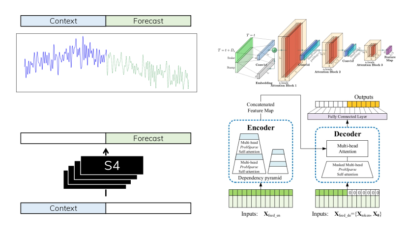
Learning with weaker inductive bias. Beyond our results on speech (Section 4.2), we further validate that S4 can be applied with minimal modifications on two domains that typically require specialized domain-specific preprocessing and architectures. First, we compare S4 to the Informer [50], a new Transformer architecture that uses a complex encoder-decoder designed for time-series forecasting problems. A simple application of S4 that treats forecasting as a masked sequence-to-sequence transformation (Fig. 11) outperforms the Informer and other baselines on settings across forecasting tasks. Notably, S4 is better on the longest setting in each task, e.g. reducing MSE by when forecasting days of weather data (Table 3).
Finally, we evaluate S4 on pixel-level sequential image classification tasks (Fig. 6), popular benchmarks which were originally LRD tests for RNNs [1]. Beyond LRDs, these benchmarks point to a recent effort of the ML community to solve vision problems with reduced domain knowledge, in the spirit of models such as Vision Transformers [12] and MLP-Mixer [41] which involve patch-based models that without 2-D inductive bias. Sequential CIFAR is a particularly challenging dataset where outside of SSMs, all sequence models have a gap of over to a simple 2-D CNN. By contrast, S4 is competitive with a larger ResNet18 (7.9M vs. 11.0M parameters), both with (93.16% vs. 95.62%) or without (91.12% vs. 89.46%) data augmentation. Moreover, it is much more robust to other architectural choices (e.g. 90.46% vs. 79.52% when swapping BatchNorm for LayerNorm).
4.4 SSM Ablations: the Importance of HiPPO
A critical motivation of S4 was the use of the HiPPO matrices to initialize an SSM. We consider several simplifications of S4 to ablate the importance of each of these components, including: (i) how important is the HiPPO initialization? (ii) how important is training the SSM on top of HiPPO? (iii) are the benefits of S4 captured by the NPLR parameterization without HiPPO?
As a simple testbed, all experiments in this section were performed on the sequential CIFAR-10 task, whicih we found transferred well to other settings. Models were constrained to at most 100K trainable parameters and trained with a simple plateau learning rate scheduler and no regularization.
Unconstrained SSMs.
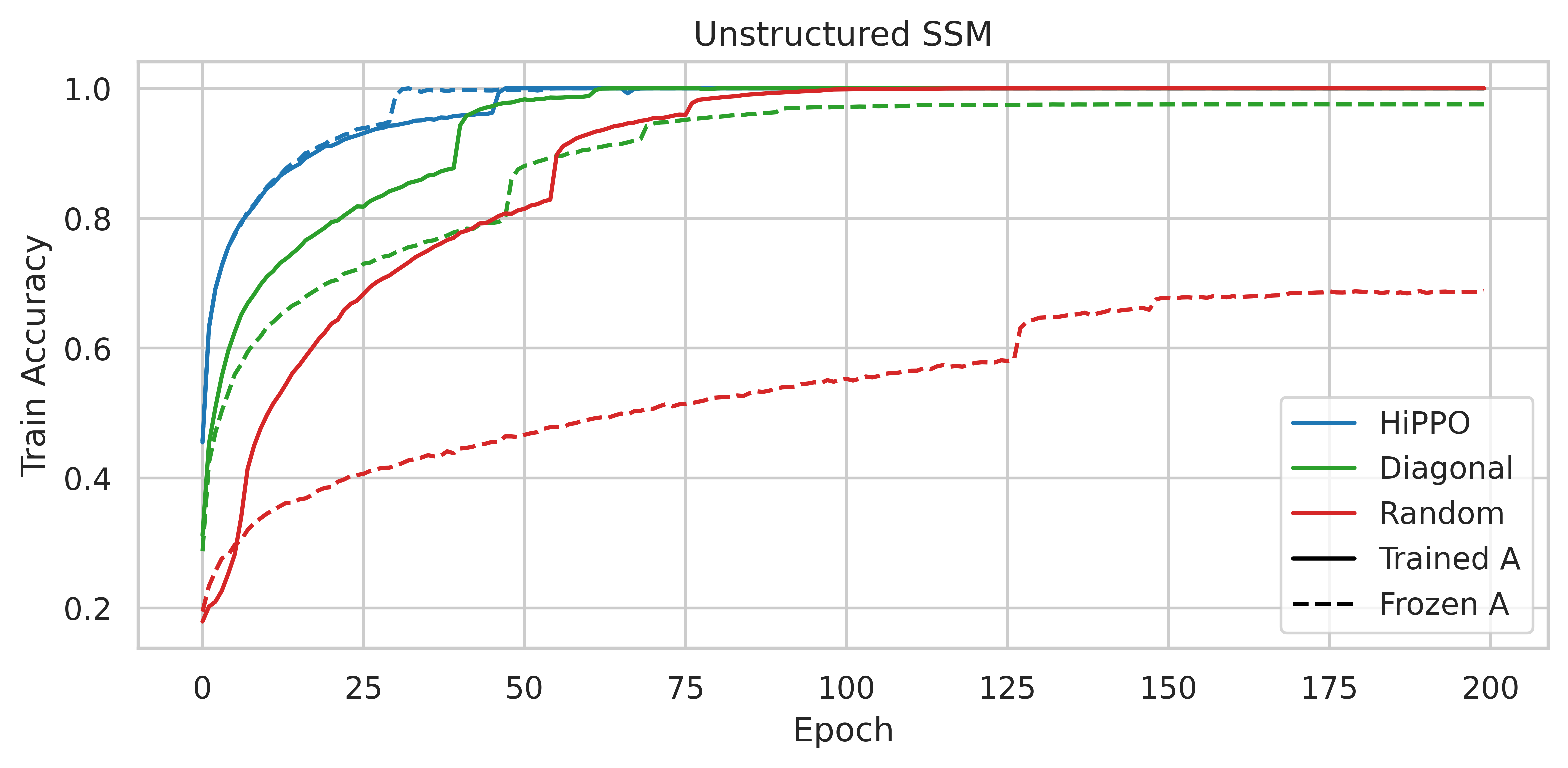
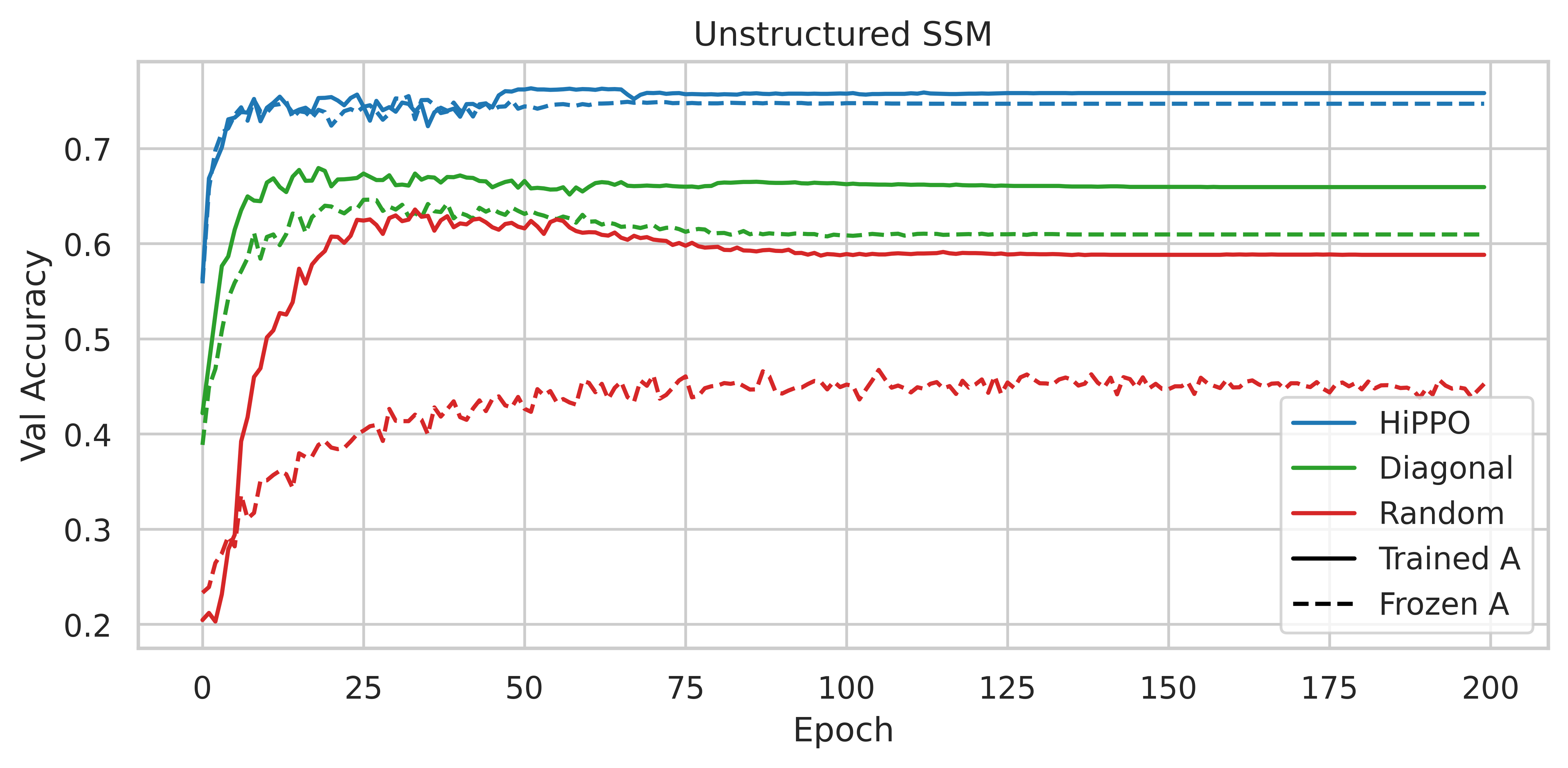
We first investigate generic SSMs with various initializations. We consider a random Gaussian initialization (with variance scaled down until it did not NaN), and the HiPPO initialization. We also consider a random diagonal Gaussian matrix as a potential structured method; parameterizing as a diagonal matrix would allow substantial speedups without going through the complexity of S4’s NPLR parameterization. We consider both freezing the matrix and training it.
Fig. 9 shows both training and validation curves, from which we can make several observations. First, training the SSM improved all methods, particularly the randomly initialized ones. For all methods, training the SSM led to improvements in both training and validation curves.
Second, a large generalization gap exists between the initializations. In particular, note that when is trained, all initializations are able to reach perfect training accuracy. However, their validation accuracies are separated by over .
NPLR SSMs.
The previous experiment validates the importance of HiPPO in SSMs. This was the main motivation of the NPLR algorithm in S4, which utilizes structure of the HiPPO matrix (2) to make SSMs computationally feasible. Fig. 10(a) shows that random NPLR matrices still do not perform well, which validates that S4’s effectiveness primarily comes from the HiPPO initialization, not the NPLR parameterization.
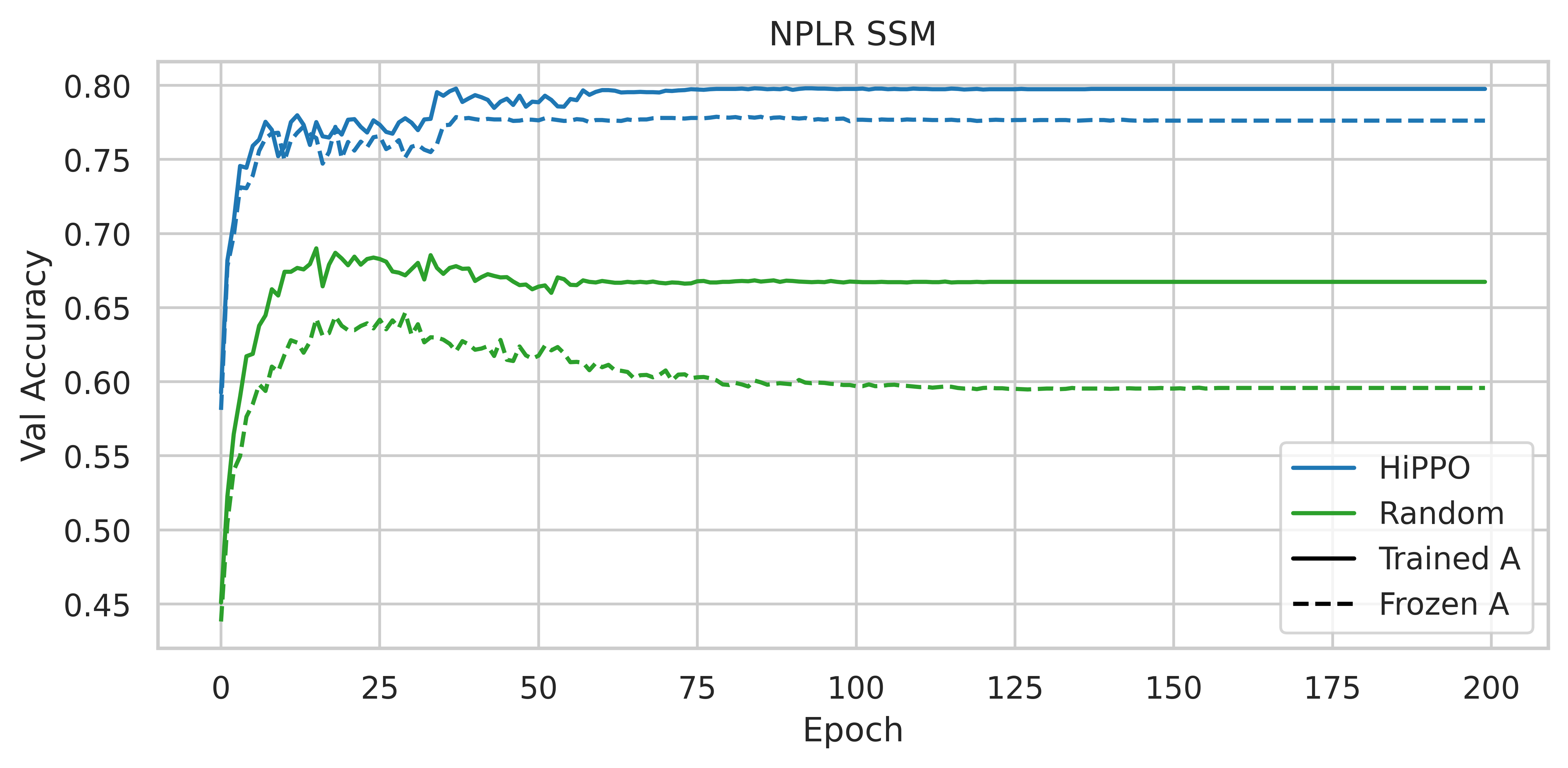
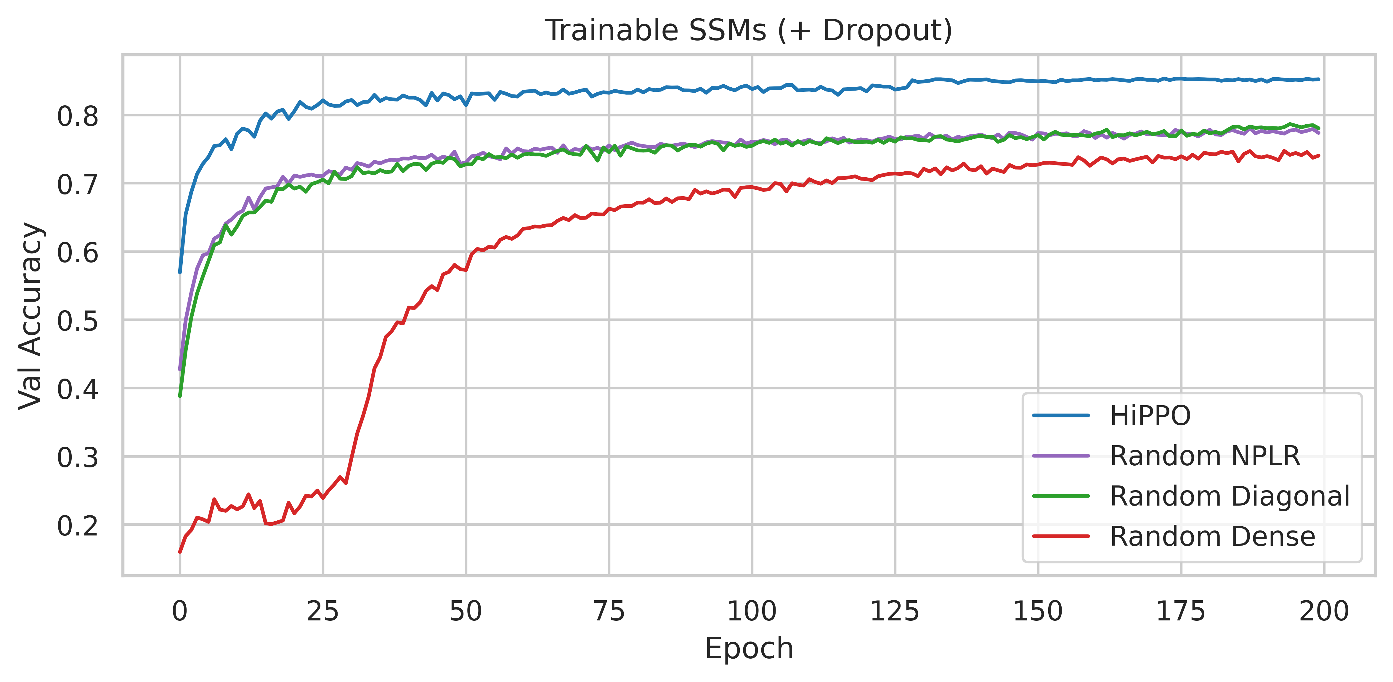
Finally, Fig. 10(b) considers the main ablations considered in this section (with trainable SSMs) and adds minor regularization. With 0.1 Dropout, the same trends still hold, and the HiPPO initialization—in other words, the full S4 method—achieves test accuracy with just 100K parameters.
5 Conclusion
We introduce S4, a sequence model that uses a new parameterization for the state space model’s continuous-time, recurrent, and convolutional views to efficiently model LRDs in a principled manner. Results across established benchmarks evaluating a diverse range of data modalities and model capabilities suggest that S4 has the potential to be an effective general sequence modeling solution.
Acknowledgments
We thank Aditya Grover and Chris Cundy for helpful discussions about earlier versions of the method. We thank Simran Arora, Sabri Eyuboglu, Bibek Paudel, and Nimit Sohoni for valuable feedback on earlier drafts of this work. This work was done with the support of Google Cloud credits under HAI proposals 540994170283 and 578192719349. We gratefully acknowledge the support of NIH under No. U54EB020405 (Mobilize), NSF under Nos. CCF1763315 (Beyond Sparsity), CCF1563078 (Volume to Velocity), and 1937301 (RTML); ONR under No. N000141712266 (Unifying Weak Supervision); ONR N00014-20-1-2480: Understanding and Applying Non-Euclidean Geometry in Machine Learning; N000142012275 (NEPTUNE); the Moore Foundation, NXP, Xilinx, LETI-CEA, Intel, IBM, Microsoft, NEC, Toshiba, TSMC, ARM, Hitachi, BASF, Accenture, Ericsson, Qualcomm, Analog Devices, the Okawa Foundation, American Family Insurance, Google Cloud, Salesforce, Total, the HAI-AWS Cloud Credits for Research program, the Stanford Data Science Initiative (SDSI), and members of the Stanford DAWN project: Facebook, Google, and VMWare. The Mobilize Center is a Biomedical Technology Resource Center, funded by the NIH National Institute of Biomedical Imaging and Bioengineering through Grant P41EB027060. The U.S. Government is authorized to reproduce and distribute reprints for Governmental purposes notwithstanding any copyright notation thereon. Any opinions, findings, and conclusions or recommendations expressed in this material are those of the authors and do not necessarily reflect the views, policies, or endorsements, either expressed or implied, of NIH, ONR, or the U.S. Government.
References
- Arjovsky et al. [2016] Martin Arjovsky, Amar Shah, and Yoshua Bengio. Unitary evolution recurrent neural networks. In The International Conference on Machine Learning (ICML), pages 1120–1128, 2016.
- Baevski and Auli [2018] Alexei Baevski and Michael Auli. Adaptive input representations for neural language modeling. arXiv preprint arXiv:1809.10853, 2018.
- Bai et al. [2018] Shaojie Bai, J Zico Kolter, and Vladlen Koltun. An empirical evaluation of generic convolutional and recurrent networks for sequence modeling. arXiv preprint arXiv:1803.01271, 2018.
- Bai et al. [2019] Shaojie Bai, J Zico Kolter, and Vladlen Koltun. Trellis networks for sequence modeling. In The International Conference on Learning Representations (ICLR), 2019.
- Chang et al. [2017] Shiyu Chang, Yang Zhang, Wei Han, Mo Yu, Xiaoxiao Guo, Wei Tan, Xiaodong Cui, Michael Witbrock, Mark Hasegawa-Johnson, and Thomas S Huang. Dilated recurrent neural networks. In Advances in Neural Information Processing Systems (NeurIPS), 2017.
- Child et al. [2019] Rewon Child, Scott Gray, Alec Radford, and Ilya Sutskever. Generating long sequences with sparse transformers. arXiv preprint arXiv:1904.10509, 2019.
- Chilkuri and Eliasmith [2021] Narsimha Chilkuri and Chris Eliasmith. Parallelizing legendre memory unit training. The International Conference on Machine Learning (ICML), 2021.
- Choromanski et al. [2020] Krzysztof Choromanski, Valerii Likhosherstov, David Dohan, Xingyou Song, Andreea Gane, Tamas Sarlos, Peter Hawkins, Jared Davis, Afroz Mohiuddin, Lukasz Kaiser, et al. Rethinking attention with performers. In The International Conference on Learning Representations (ICLR), 2020.
- Dauphin et al. [2017] Yann N Dauphin, Angela Fan, Michael Auli, and David Grangier. Language modeling with gated convolutional networks. In International conference on machine learning, pages 933–941. PMLR, 2017.
- De Brouwer et al. [2019] Edward De Brouwer, Jaak Simm, Adam Arany, and Yves Moreau. Gru-ode-bayes: Continuous modeling of sporadically-observed time series. In Advances in Neural Information Processing Systems (NeurIPS), 2019.
- Donahue et al. [2019] Chris Donahue, Julian McAuley, and Miller Puckette. Adversarial audio synthesis. In ICLR, 2019.
- Dosovitskiy et al. [2020] Alexey Dosovitskiy, Lucas Beyer, Alexander Kolesnikov, Dirk Weissenborn, Xiaohua Zhai, Thomas Unterthiner, Mostafa Dehghani, Matthias Minderer, Georg Heigold, Sylvain Gelly, et al. An image is worth 16x16 words: Transformers for image recognition at scale. arXiv preprint arXiv:2010.11929, 2020.
- Erichson et al. [2021] N Benjamin Erichson, Omri Azencot, Alejandro Queiruga, Liam Hodgkinson, and Michael W Mahoney. Lipschitz recurrent neural networks. In International Conference on Learning Representations, 2021.
- Goel et al. [2022] Karan Goel, Albert Gu, Chris Donahue, and Christopher Ré. It’s raw! audio generation with state-space models. arXiv preprint arXiv:2202.09729, 2022.
- Golub and Van Loan [2013] Gene H Golub and Charles F Van Loan. Matrix computations, volume 3. JHU press, 2013.
- Gu et al. [2020a] Albert Gu, Tri Dao, Stefano Ermon, Atri Rudra, and Christopher Ré. Hippo: Recurrent memory with optimal polynomial projections. In Advances in Neural Information Processing Systems (NeurIPS), 2020a.
- Gu et al. [2020b] Albert Gu, Caglar Gulcehre, Tom Le Paine, Matt Hoffman, and Razvan Pascanu. Improving the gating mechanism of recurrent neural networks. In The International Conference on Machine Learning (ICML), 2020b.
- Gu et al. [2021] Albert Gu, Isys Johnson, Karan Goel, Khaled Saab, Tri Dao, Atri Rudra, and Christopher Ré. Combining recurrent, convolutional, and continuous-time models with the structured learnable linear state space layer. In Advances in Neural Information Processing Systems (NeurIPS), 2021.
- Gu et al. [2022a] Albert Gu, Ankit Gupta, Karan Goel, and Christopher Ré. On the parameterization and initialization of diagonal state space models. arXiv preprint arXiv:2206.11893, 2022a.
- Gu et al. [2022b] Albert Gu, Isys Johnson, Aman Timalsina, Atri Rudra, and Christopher Ré. How to train your hippo: State space models with generalized basis projections. arXiv preprint arXiv:2206.12037, 2022b.
- Hochreiter and Schmidhuber [1997] Sepp Hochreiter and Jürgen Schmidhuber. Long short-term memory. Neural computation, 9(8):1735–1780, 1997.
- Katharopoulos et al. [2020] Angelos Katharopoulos, Apoorv Vyas, Nikolaos Pappas, and François Fleuret. Transformers are rnns: Fast autoregressive transformers with linear attention. In International Conference on Machine Learning, pages 5156–5165. PMLR, 2020.
- Kidger et al. [2020] Patrick Kidger, James Morrill, James Foster, and Terry Lyons. Neural controlled differential equations for irregular time series. arXiv preprint arXiv:2005.08926, 2020.
- Lezcano-Casado and Martínez-Rubio [2019] Mario Lezcano-Casado and David Martínez-Rubio. Cheap orthogonal constraints in neural networks: A simple parametrization of the orthogonal and unitary group. In The International Conference on Machine Learning (ICML), 2019.
- Li et al. [2018] Shuai Li, Wanqing Li, Chris Cook, Ce Zhu, and Yanbo Gao. Independently recurrent neural network (IndRNN): Building a longer and deeper RNN. In Proceedings of the IEEE Conference on Computer Vision and Pattern Recognition, pages 5457–5466, 2018.
- Lioutas and Guo [2020] Vasileios Lioutas and Yuhong Guo. Time-aware large kernel convolutions. In International Conference on Machine Learning, pages 6172–6183. PMLR, 2020.
- Merity et al. [2018] Stephen Merity, Nitish Shirish Keskar, James Bradbury, and Richard Socher. Scalable language modeling: Wikitext-103 on a single gpu in 12 hours. SysML, 2018.
- Oord et al. [2016] Aaron van den Oord, Sander Dieleman, Heiga Zen, Karen Simonyan, Oriol Vinyals, Alex Graves, Nal Kalchbrenner, Andrew Senior, and Koray Kavukcuoglu. Wavenet: A generative model for raw audio. arXiv preprint arXiv:1609.03499, 2016.
- Pan [2001] Victor Pan. Structured matrices and polynomials: unified superfast algorithms. Springer Science & Business Media, 2001.
- Pan [2017] Victor Pan. Fast approximate computations with cauchy matrices and polynomials. Mathematics of Computation, 86(308):2799–2826, 2017.
- Pan [2015] Victor Y Pan. Transformations of matrix structures work again. Linear Algebra and Its Applications, 465:107–138, 2015.
- Pascanu et al. [2013] Razvan Pascanu, Tomas Mikolov, and Yoshua Bengio. On the difficulty of training recurrent neural networks. In International conference on machine learning, pages 1310–1318, 2013.
- Rae et al. [2018] Jack Rae, Chris Dyer, Peter Dayan, and Timothy Lillicrap. Fast parametric learning with activation memorization. The International Conference on Machine Learning (ICML), 2018.
- Ramachandran et al. [2017] Prajit Ramachandran, Tom Le Paine, Pooya Khorrami, Mohammad Babaeizadeh, Shiyu Chang, Yang Zhang, Mark A Hasegawa-Johnson, Roy H Campbell, and Thomas S Huang. Fast generation for convolutional autoregressive models. arXiv preprint arXiv:1704.06001, 2017.
- Romero et al. [2021] David W Romero, Anna Kuzina, Erik J Bekkers, Jakub M Tomczak, and Mark Hoogendoorn. Ckconv: Continuous kernel convolution for sequential data. arXiv preprint arXiv:2102.02611, 2021.
- Romero et al. [2022] David W Romero, Robert-Jan Bruintjes, Jakub M Tomczak, Erik J Bekkers, Mark Hoogendoorn, and Jan C van Gemert. Flexconv: Continuous kernel convolutions with differentiable kernel sizes. In The International Conference on Learning Representations (ICLR), 2022.
- Rubanova et al. [2019] Yulia Rubanova, Tian Qi Chen, and David K Duvenaud. Latent ordinary differential equations for irregularly-sampled time series. In Advances in Neural Information Processing Systems, pages 5321–5331, 2019.
- Rusch and Mishra [2021] T Konstantin Rusch and Siddhartha Mishra. Unicornn: A recurrent model for learning very long time dependencies. The International Conference on Machine Learning (ICML), 2021.
- Salimans et al. [2017] Tim Salimans, Andrej Karpathy, Xi Chen, and Diederik P Kingma. Pixelcnn++: Improving the pixelcnn with discretized logistic mixture likelihood and other modifications. arXiv preprint arXiv:1701.05517, 2017.
- Tay et al. [2021] Yi Tay, Mostafa Dehghani, Samira Abnar, Yikang Shen, Dara Bahri, Philip Pham, Jinfeng Rao, Liu Yang, Sebastian Ruder, and Donald Metzler. Long range arena : A benchmark for efficient transformers. In International Conference on Learning Representations, 2021. URL https://openreview.net/forum?id=qVyeW-grC2k.
- Tolstikhin et al. [2021] Ilya Tolstikhin, Neil Houlsby, Alexander Kolesnikov, Lucas Beyer, Xiaohua Zhai, Thomas Unterthiner, Jessica Yung, Daniel Keysers, Jakob Uszkoreit, Mario Lucic, et al. Mlp-mixer: An all-mlp architecture for vision. arXiv preprint arXiv:2105.01601, 2021.
- Trinh et al. [2018] Trieu H Trinh, Andrew M Dai, Minh-Thang Luong, and Quoc V Le. Learning longer-term dependencies in RNNs with auxiliary losses. In The International Conference on Machine Learning (ICML), 2018.
- Tustin [1947] Arnold Tustin. A method of analysing the behaviour of linear systems in terms of time series. Journal of the Institution of Electrical Engineers-Part IIA: Automatic Regulators and Servo Mechanisms, 94(1):130–142, 1947.
- Vaswani et al. [2017] Ashish Vaswani, Noam Shazeer, Niki Parmar, Jakob Uszkoreit, Llion Jones, Aidan N. Gomez, Lukasz Kaiser, and Illia Polosukhin. Attention is all you need. In Advances in Neural Information Processing Systems (NeurIPS), 2017.
- Voelker et al. [2019] Aaron Voelker, Ivana Kajić, and Chris Eliasmith. Legendre memory units: Continuous-time representation in recurrent neural networks. In Advances in Neural Information Processing Systems, pages 15544–15553, 2019.
- Voelker [2019] Aaron Russell Voelker. Dynamical systems in spiking neuromorphic hardware. PhD thesis, University of Waterloo, 2019.
- Warden [2018] Pete Warden. Speech commands: A dataset for limited-vocabulary speech recognition. ArXiv, abs/1804.03209, 2018.
- Woodbury [1950] Max A Woodbury. Inverting modified matrices. Memorandum report, 42:106, 1950.
- Wu et al. [2019] Felix Wu, Angela Fan, Alexei Baevski, Yann N Dauphin, and Michael Auli. Pay less attention with lightweight and dynamic convolutions. In The International Conference on Learning Representations (ICLR), 2019.
- Zhou et al. [2021] Haoyi Zhou, Shanghang Zhang, Jieqi Peng, Shuai Zhang, Jianxin Li, Hui Xiong, and Wancai Zhang. Informer: Beyond efficient transformer for long sequence time-series forecasting. In The Thirty-Fifth AAAI Conference on Artificial Intelligence, AAAI 2021, Virtual Conference, volume 35, pages 11106–11115. AAAI Press, 2021.
Appendix A Discussion
Related Work.
Our work is most closely related to a line of work originally motivated by a particular biologically-inspired SSM, which led to mathematical models for addressing LRDs. Voelker [46], Voelker et al. [45] derived a non-trainable SSM motivated from approximating a neuromorphic spiking model, and Chilkuri and Eliasmith [7] showed that it could be sped up at train time with a convolutional view. Gu et al. [16] extended this special case to a general continuous-time function approximation framework with several more special cases of matrices designed for long-range dependencies. However, instead of using a true SSM, all of these works fixed a choice of and built RNNs around it. Most recently, Gu et al. [18] used the full (1) explicitly as a deep SSM model, exploring new conceptual views of SSMs, as well as allowing to be trained. As mentioned in Section 1, their method used a naive instantiation of SSMs that suffered from an additional factor of in memory and in computation.
Beyond this work, our technical contributions (Section 3) on the S4 parameterization and algorithms are applicable to a broader family of SSMs including these investigated in prior works, and our techniques for working with these models may be of independent interest.
Implementation.
The computational core of S4’s training algorithm is the Cauchy kernel discussed in Sections 3.2, 3.3 and C.3. As described in Section C.3 Proposition 5, there are many algorithms for it with differing computational complexities and sophistication. Our current implementation of S4 actually uses the naive algorithm which is easily parallelized on GPUs and has more easily accessible libraries allowing it to be implemented; we leverage the pykeops library for memory-efficient kernel operations. However, this library is a much more general library that may not be optimized for the Cauchy kernels used here, and we believe that a dedicated CUDA implementation can be more efficient. Additionally, as discussed in this work, there are asymptotically faster and numerically stable algorithms for the Cauchy kernel (Proposition 5). However, these algorithms are currently not implemented for GPUs due to a lack of previous applications that require them. We believe that more efficient implementations of these self-contained computational kernels are possible, and that S4 (and SSMs at large) may have significant room for further improvements in efficiency.
Limitations and Future Directions.
In this work, we show that S4 can address a wide variety of data effectively. However, it may not necessarily be the most suitable model for all types of data. For example, Fig. 8 still found a gap compared to Transformers for language modeling. An interesting future direction is exploring combinations of S4 with other sequence models to complement their strengths. We are excited about other directions, including continuing to explore the benefits of S4 on audio data (e.g. pre-training or generation settings), and generalizing HiPPO and S4 to higher-dimensional data for image and video applications.
Appendix B Numerical Instability of LSSL
This section proves the claims made in Section 3.1 about prior work. We first derive the explicit diagonalization of the HiPPO matrix, confirming its instability because of exponentially large entries. We then discuss the proposed theoretically fast algorithm from [18] (Theorem 2) and show that it also involves exponentially large terms and thus cannot be implemented.
B.1 HiPPO Diagonalization
Proof of Lemma 3.2.
The HiPPO matrix (2) is equal, up to sign and conjugation by a diagonal matrix, to
Our goal is to show that this is diagonalized by the matrix
or in other words that columns of this matrix are eigenvectors of .
Concretely, we will show that the -th column of this matrix with elements
is an eigenvector with eigenvalue . In other words we must show that for all indices ,
| (7) |
If , then for all inside the sum, either or . In the first case and in the second case , so both sides of equation (7) are equal to .
It remains to show the case , which proceeds by induction on . Expanding equation (7) using the formula for yields
In the base case , the sum disappears and we are left with , as desired.
Otherwise, the sum for is the same as the sum for but with sign reversed and a few edge terms. The result follows from applying the inductive hypothesis and algebraic simplification:
∎
B.2 Fast but Unstable LSSL Algorithm
Instead of diagonalization, Gu et al. [18, Theorem 2] proposed a sophisticated fast algorithm to compute
This algorithm runs in operations and space. However, we now show that this algorithm is also numerically unstable.
There are several reasons for the instability of this algorithm, but most directly we can pinpoint a particular intermediate quantity that they use.
Definition 1.
The fast LSSL algorithm computes coefficients of , the characteristic polynomial of , as an intermediate computation. Additionally, it computes the coefficients of its inverse, .
We now claim that this quantity is numerically unfeasible. We narrow down to the case when is the identity matrix. Note that this case is actually in some sense the most typical case: when discretizing the continuous-time SSM to discrete-time by a step-size , the discretized transition matrix is brought closer to the identity. For example, with the Euler discretization , we have as the step size .
Lemma B.1.
When , the fast LSSL algorithm requires computing terms exponentially large in .
Proof.
The characteristic polynomial of is
These coefficients have size up to .
The inverse of has even larger coefficients. It can be calculated in closed form by the generalized binomial formula:
Taking this , the largest coefficient is
When this is
already larger than the coefficients of , and only increases as grows. ∎
Appendix C S4 Algorithm Details
This section proves the results of Section 3.3, providing complete details of our efficient algorithms for S4.
Sections C.1, C.2 and C.3 prove Theorems 1, 2 and 3 respectively.
C.1 NPLR Representations of HiPPO Matrices
We first prove Theorem 1, showing that all HiPPO matrices for continuous-time memory fall under the S4 normal plus low-rank (NPLR) representation.
Proof of Theorem 1.
We consider each of the three cases HiPPO-LagT, HiPPO-LegT, and HiPPO-LegS separately. Note that the primary HiPPO matrix defined in this work (equation (2)) is the HiPPO-LegT matrix.
HiPPO-LagT. The HiPPO-LagT matrix is simply
Adding the matrix of all , which is rank 1, yields
This matrix is now skew-symmetric. Skew-symmetric matrices are a particular case of normal matrices with pure-imaginary eigenvalues.
Gu et al. [16] also consider a case of HiPPO corresponding to the generalized Laguerre polynomials that generalizes the above HiPPO-LagT case. In this case, the matrix (up to conjugation by a diagonal matrix) ends up being close to the above matrix, but with a different element on the diagonal. After adding the rank-1 correction, it becomes the above skew-symmetric matrix plus a multiple of the identity. Thus after diagonalization by the same matrix as in the LagT case, it is still reduced to diagonal plus low-rank (DPLR) form, where the diagonal is now pure imaginary plus a real constant.
HiPPO-LegS. We restate the formula from equation (2) for convenience.
Adding to the whole matrix gives
Note that this matrix is not skew-symmetric, but is where is a skew-symmetric matrix. This is diagonalizable by the same unitary matrix that diagonalizes .
HiPPO-LegT.
Up to the diagonal scaling, the LegT matrix is
By adding to this matrix and then the matrix
the matrix becomes
which is skew-symmetric. In fact, this matrix is the inverse of the Chebyshev Jacobi.
An alternative way to see this is as follows. The LegT matrix is the inverse of the matrix
This can obviously be converted to a skew-symmetric matrix by adding a rank 2 term. The inverses of these matrices are also rank-2 differences from each other by the Woodbury identity.
A final form is
This has the advantage that the rank-2 correction is symmetric (like the others), but the normal skew-symmetric matrix is now -quasiseparable instead of -quasiseparable.
∎
C.2 Computing the S4 Recurrent View
We prove Theorem 2 showing the efficiency of the S4 parameterization for computing one step of the recurrent representation (Section 2.3).
Recall that without loss of generality, we can assume that the state matrix is diagonal plus low-rank (DPLR), potentially over . Our goal in this section is to explicitly write out a closed form for the discretized matrix .
Recall from equation (3) that
We first simplify both terms in the definition of independently.
Forward discretization. The first term is essentially the Euler discretization motivated in Section 2.3.
where is defined as the term in the final brackets.
Backward discretization. The second term is known as the Backward Euler’s method. Although this inverse term is normally difficult to deal with, in the DPLR case we can simplify it using Woodbury’s Identity (Proposition 4).
where and is defined as the term in the final brackets. Note that is actually a scalar in the case when the low-rank term has rank .
C.3 Computing the Convolutional View
The most involved part of using SSMs efficiently is computing . This algorithm was sketched in Section 3.2 and is the main motivation for the S4 parameterization. In this section, we define the necessary intermediate quantities and prove the main technical result.
The algorithm for Theorem 3 falls in roughly three stages, leading to Algorithm 1. Assuming has been conjugated into diagonal plus low-rank form, we successively simplify the problem of computing by applying the techniques outlined in Section 3.2.
Remark C.1.
We note that for the remainder of this section, we transpose to be a column vector of shape or instead of matrix or row vector as in (1). In other words the SSM is
| (8) | ||||
This convention is made so that has the same shape as and simplifies the implementation of S4.
Reduction 0: Diagonalization
By Lemma 3.1, we can switch the representation by conjugating with any unitary matrix. For the remainder of this section, we can assume that is (complex) diagonal plus low-rank (DPLR).
Note that unlike diagonal matrices, a DPLR matrix does not lend itself to efficient computation of . The reason is that computes terms which involve powers of the matrix . These are trivially computable when is diagonal, but is no longer possible for even simple modifications to diagonal matrices such as DPLR.
Reduction 1: SSM Generating Function
To address the problem of computing powers of , we introduce another technique. Instead of computing the SSM convolution filter directly, we introduce a generating function on its coefficients and compute evaluations of it.
Definition 2 (SSM Generating Function).
We define the following quantities:
-
•
The SSM convolution function is and the (truncated) SSM filter of length
(9) -
•
The SSM generating function at node is
(10) and the truncated SSM generating function at node is
(11) -
•
The truncated SSM generating function at nodes is
(12)
Intuitively, the generating function essentially converts the SSM convolution filter from the time domain to frequency domain. Importantly, it preserves the same information, and the desired SSM convolution filter can be recovered from evaluations of its generating function.
Lemma C.2.
The SSM function can be computed from the SSM generating function at the roots of unity stably in operations.
Proof.
For convenience define
Note that
Note that this is exactly the same as the Discrete Fourier Transform (DFT):
Therefore can be recovered from with a single inverse DFT, which requires operations with the Fast Fourier Transform (FFT) algorithm. ∎
Reduction 2: Woodbury Correction
The primary motivation of Definition 2 is that it turns powers of into a single inverse of (equation (10)). While DPLR matrices cannot be powered efficiently due to the low-rank term, they can be inverted efficiently by the well-known Woodbury identity.
Proposition 4 (Binomial Inverse Theorem or Woodbury matrix identity [48, 15]).
Over a commutative ring , let and . Suppose and are invertible. Then is invertible and
With this identity, we can convert the SSM generating function on a DPLR matrix into one on just its diagonal component.
Lemma C.3.
Let be a diagonal plus low-rank representation. Then for any root of unity , the truncated generating function satisfies
Proof.
We can now explicitly expand the discretized SSM matrices and back in terms of the original SSM parameters and . Lemma C.4 provides an explicit formula, which allows further simplifying
The last line applies the Woodbury Identity (Proposition 4) where . ∎
The previous proof used the following self-contained result to back out the original SSM matrices from the discretization.
Lemma C.4.
Let be the SSM matrices discretized by the bilinear discretization with step size . Then
Proof.
Recall that the bilinear discretization that we use (equation (3)) is
The result is proved algebraic manipulations.
∎
Note that in the S4 parameterization, instead of constantly computing , we can simply reparameterize our parameters to learn directly instead of , saving a minor computation cost and simplifying the algorithm.
Reduction 3: Cauchy Kernel
We have reduced the original problem of computing to the problem of computing the SSM generating function in the case that is a diagonal matrix. We show that this is exactly the same as a Cauchy kernel, which is a well-studied problem with fast and stable numerical algorithms.
Definition 3.
A Cauchy matrix or kernel on nodes and is
The computation time of a Cauchy matrix-vector product of size is denoted by .
Computing with Cauchy matrices is an extremely well-studied problem in numerical analysis, with both fast arithmetic algorithms and fast numerical algorithms based on the famous Fast Multipole Method (FMM) [29, 31, 30].
Proposition 5 (Cauchy).
A Cauchy kernel requires space, and operation count
Corollary C.5.
Evaluating (defined in Lemma C.3) for any set of nodes , diagonal matrix , and vectors can be computed in operations and space, where is the cost of a Cauchy matrix-vector multiplication.
Proof.
For any fixed , we want to compute . Computing this over all is therefore exactly a Cauchy matrix-vector multiplication. ∎
This completes the proof of Theorem 3. In Algorithm 1, note that the work is dominated by Step 4, which has a constant number of calls to a black-box Cauchy kernel, with complexity given by Proposition 5.
Appendix D Experiment Details and Full Results
This section contains full experimental procedures and extended results and citations for our experimental evaluation in Section 4. Section D.1 corresponds to benchmarking results in Section 4.1, Section D.2 corresponds to LRD experiments (LRA and Speech Commands) in Section 4.2, and Section D.3 corresponds to the general sequence modeling experiments (generation, image classification, forecasting) in Section 4.3.
D.1 Benchmarking
Benchmarks against LSSL
For a given dimension , a single LSSL or S4 layer was constructed with hidden features. For LSSL, the state size was set to as done in [18]. For S4, the state size was set to parameter-match the LSSL, which was a state size of due to differences in the parameterization. Fig. 3 benchmarks a single forward+backward pass of a single layer.
Benchmarks against Efficient Transformers
Following [40], the Transformer models had 4 layers, hidden dimension with heads, query/key/value projection dimension , and batch size , for a total of roughly parameters. The S4 model was parameter tied while keeping the depth and hidden dimension constant (leading to a state size of ).
We note that the relative orderings of these methods can vary depending on the exact hyperparameter settings.
D.2 Long-Range Dependencies
This section includes information for reproducing our experiments on the Long-Range Arena and Speech Commands long-range dependency tasks.
Long Range Arena
| Model | ListOps | Text | Retrieval | Image | Pathfinder | Path-X | Avg |
|---|---|---|---|---|---|---|---|
| Random | 10.00 | 50.00 | 50.00 | 10.00 | 50.00 | 50.00 | 36.67 |
| Transformer | 36.37 | 64.27 | 57.46 | 42.44 | 71.40 | ✗ | 53.66 |
| Local Attention | 15.82 | 52.98 | 53.39 | 41.46 | 66.63 | ✗ | 46.71 |
| Sparse Trans. | 17.07 | 63.58 | 59.59 | 44.24 | 71.71 | ✗ | 51.03 |
| Longformer | 35.63 | 62.85 | 56.89 | 42.22 | 69.71 | ✗ | 52.88 |
| Linformer | 35.70 | 53.94 | 52.27 | 38.56 | 76.34 | ✗ | 51.14 |
| Reformer | 37.27 | 56.10 | 53.40 | 38.07 | 68.50 | ✗ | 50.56 |
| Sinkhorn Trans. | 33.67 | 61.20 | 53.83 | 41.23 | 67.45 | ✗ | 51.23 |
| Synthesizer | 36.99 | 61.68 | 54.67 | 41.61 | 69.45 | ✗ | 52.40 |
| BigBird | 36.05 | 64.02 | 59.29 | 40.83 | 74.87 | ✗ | 54.17 |
| Linear Trans. | 16.13 | 65.90 | 53.09 | 42.34 | 75.30 | ✗ | 50.46 |
| Performer | 18.01 | 65.40 | 53.82 | 42.77 | 77.05 | ✗ | 51.18 |
| FNet | 35.33 | 65.11 | 59.61 | 38.67 | 77.80 | ✗ | 54.42 |
| Nyströmformer | 37.15 | 65.52 | 79.56 | 41.58 | 70.94 | ✗ | 57.46 |
| Luna-256 | 37.25 | 64.57 | 79.29 | 47.38 | 77.72 | ✗ | 59.37 |
| S4 (original) | 58.35 | 76.02 | 87.09 | 87.26 | 86.05 | 88.10 | 80.48 |
| S4 (updated) | 59.60 | 86.82 | 90.90 | 88.65 | 94.20 | 96.35 | 86.09 |
For the S4 model, hyperparameters for all datasets are reported in Table 5. For all datasets, we used the AdamW optimizer with a constant learning rate schedule with decay on validation plateau. However, the learning rate on HiPPO parameters (in particular ) were reduced to a maximum starting LR of , which improves stability since the HiPPO equation is crucial to performance.
The S4 state size was always fixed to .
As S4 is a sequence-to-sequence model with output shape (batch, length, dimension) and LRA tasks are classification, mean pooling along the length dimension was applied after the last layer.
We note that most of these results were trained for far longer than what was necessary to achieve SotA results (e.g., the Image task reaches SotA in 1 epoch). Results often keep improving with longer training times.
Updated results. The above hyperparameters describe the results reported in the original paper, shown in Table 4, which have since been improved. See Section D.5.
Hardware. All models were run on single GPU. Some tasks used an A100 GPU (notably, the Path-X experiments), which has a larger max memory of 40Gb. To reproduce these on smaller GPUs, the batch size can be reduced or gradients can be accumulated for two batches.
| Depth | Features | Norm | Pre-norm | Dropout | LR | Batch Size | Epochs | WD | Patience | |
| ListOps | 6 | 128 | BN | False | 0 | 0.01 | 100 | 50 | 0.01 | 5 |
| Text | 4 | 64 | BN | True | 0 | 0.001 | 50 | 20 | 0 | 5 |
| Retrieval | 6 | 256 | BN | True | 0 | 0.002 | 64 | 20 | 0 | 20 |
| Image | 6 | 512 | LN | False | 0.2 | 0.004 | 50 | 200 | 0.01 | 20 |
| Pathfinder | 6 | 256 | BN | True | 0.1 | 0.004 | 100 | 200 | 0 | 10 |
| Path-X | 6 | 256 | BN | True | 0.0 | 0.0005 | 32 | 100 | 0 | 20 |
| CIFAR-10 | 6 | 1024 | LN | False | 0.25 | 0.01 | 50 | 200 | 0.01 | 20 |
| Speech Commands (MFCC) | 4 | 256 | LN | False | 0.2 | 0.01 | 100 | 50 | 0 | 5 |
| Speech Commands (Raw) | 6 | 128 | BN | True | 0.1 | 0.01 | 20 | 150 | 0 | 10 |
Speech Commands
We provide details of sweeps run for baseline methods run by us—numbers for all others method are taken from Gu et al. [18]. The best hyperparameters used for S4 are included in Table 5.
Transformer [44] For MFCC, we swept the number of model layers , dropout and learning rates . We used attention heads, model dimension , prenorm, positional encodings, and trained for epochs with a batch size of . For Raw, the Transformer model’s memory usage made training impossible.
Performer [8] For MFCC, we swept the number of model layers , dropout and learning rates . We used attention heads, model dimension , prenorm, positional encodings, and trained for epochs with a batch size of . For Raw, we used a model dimension of , attention heads, prenorm, and a batch size of . We reduced the number of model layers to , so the model would fit on the single GPU. We trained for epochs with a learning rate of and no dropout.
ExpRNN [24] For MFCC, we swept hidden sizes and learning rates . Training was run for epochs, with a single layer model using a batch size of . For Raw, we swept hidden sizes and learning rates (however, ExpRNN failed to learn).
LipschitzRNN [13] For MFCC, we swept hidden sizes and learning rates . Training was run for epochs, with a single layer model using a batch size of . For Raw, we found that LipschitzRNN was too slow to train on a single GPU (requiring a full day for epoch of training alone).
WaveGAN Discriminator [11] The WaveGAN-D in Fig. 6 is actually our improved version of the discriminator network from the recent WaveGAN model for speech [11]. This CNN actually did not work well out-of-the-box, and we added several features to help it perform better. The final model is highly specialized compared to our model, and includes:
-
•
Downsampling or pooling between layers, induced by strided convolutions, that decrease the sequence length between layers.
-
•
A global fully-connected output layer; thus the model only works for one input sequence length and does not work on MFCC features or the frequency-shift setting in Fig. 6.
-
•
Batch Normalization is essential, whereas S4 works equally well with either Batch Normalization or Layer Normalization.
-
•
Almost as many parameters as the S4 model (M vs. M).
D.3 General Sequence Modeling
This subsection corresponds to the experiments in Section 4.3. Because of the number of experiments in this section, we use subsubsection dividers for different tasks to make it easier to follow: CIFAR-10 density estimation (Section D.3.1), WikiText-103 language modeling (Section D.3.2), autoregressive generation (Section D.3.3), sequential image classification (Section D.3.4), and time-series forecasting (Section D.3.5).
D.3.1 CIFAR Density Estimation
This task used a different backbone than the rest of our experiments. We used blocks of alternating S4 layers and position-wise feed-forward layers (in the style of Transformer blocks). Each feed-forward intermediate dimension was set to the hidden size of the incoming S4 layer. Similar to Salimans et al. [39], we used a UNet-style backbone consisting of identical blocks followed by a downsampling layer. The downsampling rates were (the 3 chosen because the sequence consists of RGB pixels). The base model had with starting hidden dimension 128, while the large model had with starting hidden dimension 192.
We experimented with both the mixture of logistics from [39] as well as a simpler 256-way categorical loss. We found they were pretty close and ended up using the simpler softmax loss along with using input embeddings.
We used the LAMB optimizer with learning rate 0.005. The base model had no dropout, while the large model had dropout 0.1 before the linear layers inside the S4 and FF blocks.
D.3.2 WikiText-103 Language Modeling
The RNN baselines included in Fig. 8 are the AWD-QRNN [27], an efficient linear gated RNN, and the LSTM + Cache + Hebbian + MbPA [33], the best performing pure RNN in the literature. The CNN baselines are the CNN with GLU activations [9], the TrellisNet [4], Dynamic Convolutions [49], and TaLK Convolutions [26].
The Transformer baseline is [2], which uses Adaptive Inputs with a tied Adaptive Softmax. This model is a standard high-performing Transformer baseline on this benchmark, used for example by Lioutas and Guo [26] and many more.
Our S4 model uses the same Transformer backbone as in [2]. The model consists of 16 blocks of S4 layers alternated with position-wise feedforward layers, with a feature dimension of 1024. Because our S4 layer has around 1/4 the number of parameters as a self-attention layer with the same dimension, we made two modifications to match the parameter count better: (i) we used a GLU activation after the S4 linear layer (Section 3.4) (ii) we used two S4 layers per block. Blocks use Layer Normalization in the pre-norm position. The embedding and softmax layers were the Adaptive Embedding from [2] with standard cutoffs 20000, 40000, 200000.
Evaluation was performed similarly to the basic setting in [2], Table 5, which uses sliding non-overlapping windows. Other settings are reported in [2] that include more context at training and evaluation time and improves the score. Because such evaluation protocols are orthogonal to the basic model, we do not consider them and report the base score from [2] Table 5.
Instead of SGD+Momentum with multiple cosine learning rate annealing cycles, our S4 model was trained with the simpler AdamW optimizer with a single cosine learning rate cycle with a maximum of 800000 steps. The initial learning rate was set to 0.0005. We used 8 A100 GPUs with a batch size of 1 per gpu and context size 8192. We used no gradient clipping and a weight decay of 0.1. Unlike [2] which specified different dropout rates for different parameters, we used a constant dropout rate of 0.25 throughout the network, including before every linear layer and on the residual branches.
D.3.3 Autoregressive Generation Speed
Protocol.
To account for different model sizes and memory requirements for each method, we benchmark generation speed by throughput, measured in images per second (Fig. 8) or tokens per second (Fig. 8). Each model generates images on a single GPU, maximizing batch size to fit in memory. (For CIFAR-10 generation we limited memory to 16Gb, to be more comparable to the Transformer and Linear Transformer results reported from [22].)
Baselines.
The Transformer and Linear Transformer baselines reported in Fig. 8 are the results reported directly from Katharopoulos et al. [22]. Note that the Transformer number is the one in their Appendix, which implements the optimized cached implementation of self-attention.
For all other baseline models, we used open source implementations of the models to benchmark generation speed. For the PixelCNN++, we used the fast cached version by Ramachandran et al. [34], which sped up generation by orders of magnitude from the naive implementation. This code was only available in TensorFlow, which may have slight differences compared to the rest of the baselines which were implemented in PyTorch.
We were unable to run the Sparse Transformer [6] model due to issues with their custom CUDA implementation of the sparse attention kernel, which we were unable to resolve.
The Transformer baseline from Fig. 8 was run using a modified GPT-2 backbone from the HuggingFace repository, configured to recreate the architecture reported in [2]. These numbers are actually slightly favorable to the baseline, as we did not include the timing of the embedding or softmax layers, whereas the number reported for S4 is the full model.
D.3.4 Pixel-Level Sequential Image Classification
Our models were trained with the AdamW optimizer for up to 200 epochs. Hyperparameters for the CIFAR-10 model is reported in Table 5.
For our comparisons against ResNet-18, the main differences between the base models are that S4 uses LayerNorm by default while ResNet uses BatchNorm. The last ablation in Section 4.3 swaps the normalization type, using BatchNorm for S4 and LayerNorm for ResNet, to ablate this architectural difference. The experiments with augmentation take the base model and train with mild data augmentation: horizontal flips and random crops (with symmetric padding).
| Model | sMNIST | pMNIST | sCIFAR |
| Transformer [44, 42] | 98.9 | 97.9 | 62.2 |
| CKConv [35] | 99.32 | 98.54 | 63.74 |
| TrellisNet [4] | 99.20 | 98.13 | 73.42 |
| TCN [3] | 99.0 | 97.2 | - |
| LSTM [21, 17] | 98.9 | 95.11 | 63.01 |
| r-LSTM [42] | 98.4 | 95.2 | 72.2 |
| Dilated GRU [5] | 99.0 | 94.6 | - |
| Dilated RNN [5] | 98.0 | 96.1 | - |
| IndRNN [25] | 99.0 | 96.0 | - |
| expRNN [24] | 98.7 | 96.6 | - |
| UR-LSTM | 99.28 | 96.96 | 71.00 |
| UR-GRU [17] | 99.27 | 96.51 | 74.4 |
| LMU [45] | - | 97.15 | - |
| HiPPO-RNN [16] | 98.9 | 98.3 | 61.1 |
| UNIcoRNN [38] | - | 98.4 | - |
| LMUFFT [7] | - | 98.49 | - |
| LipschitzRNN [13] | 99.4 | 96.3 | 64.2 |
| S4 | 99.63 | 98.70 | 91.13 |
D.3.5 Time Series Forecasting compared to Informer
We include a simple figure (Fig. 11) contrasting the architecture of S4 against that of the Informer [50].
In Fig. 11, the goal is to forecast a contiguous range of future predictions (Green, length ) given a range of past context (Blue, length ). We simply concatenate the entire context with a sequence of masks set to the length of the forecast window. This input is a single sequence of length that is run through the same simple deep S4 model used throughout this work, which maps to an output of length . We then use just the last outputs as the forecasted predictions.
Tables 7 and 8 contain full results on all 50 settings considered by Zhou et al. [50]. S4 sets the best results on 40 out of 50 of these settings.
| Methods | S4 | Informer | Informer† | LogTrans | Reformer | LSTMa | DeepAR | ARIMA | Prophet | |
|---|---|---|---|---|---|---|---|---|---|---|
| Metric | MSE MAE | MSE MAE | MSE MAE | MSE MAE | MSE MAE | MSE MAE | MSE MAE | MSE MAE | MSE MAE | |
| ETTh1 | 24 | 0.061 0.191 | 0.098 0.247 | 0.092 0.246 | 0.103 0.259 | 0.222 0.389 | 0.114 0.272 | 0.107 0.280 | 0.108 0.284 | 0.115 0.275 |
| 48 | 0.079 0.220 | 0.158 0.319 | 0.161 0.322 | 0.167 0.328 | 0.284 0.445 | 0.193 0.358 | 0.162 0.327 | 0.175 0.424 | 0.168 0.330 | |
| 168 | 0.104 0.258 | 0.183 0.346 | 0.187 0.355 | 0.207 0.375 | 1.522 1.191 | 0.236 0.392 | 0.239 0.422 | 0.396 0.504 | 1.224 0.763 | |
| 336 | 0.080 0.229 | 0.222 0.387 | 0.215 0.369 | 0.230 0.398 | 1.860 1.124 | 0.590 0.698 | 0.445 0.552 | 0.468 0.593 | 1.549 1.820 | |
| 720 | 0.116 0.271 | 0.269 0.435 | 0.257 0.421 | 0.273 0.463 | 2.112 1.436 | 0.683 0.768 | 0.658 0.707 | 0.659 0.766 | 2.735 3.253 | |
| ETTh2 | 24 | 0.095 0.234 | 0.093 0.240 | 0.099 0.241 | 0.102 0.255 | 0.263 0.437 | 0.155 0.307 | 0.098 0.263 | 3.554 0.445 | 0.199 0.381 |
| 48 | 0.191 0.346 | 0.155 0.314 | 0.159 0.317 | 0.169 0.348 | 0.458 0.545 | 0.190 0.348 | 0.163 0.341 | 3.190 0.474 | 0.304 0.462 | |
| 168 | 0.167 0.333 | 0.232 0.389 | 0.235 0.390 | 0.246 0.422 | 1.029 0.879 | 0.385 0.514 | 0.255 0.414 | 2.800 0.595 | 2.145 1.068 | |
| 336 | 0.189 0.361 | 0.263 0.417 | 0.258 0.423 | 0.267 0.437 | 1.668 1.228 | 0.558 0.606 | 0.604 0.607 | 2.753 0.738 | 2.096 2.543 | |
| 720 | 0.187 0.358 | 0.277 0.431 | 0.285 0.442 | 0.303 0.493 | 2.030 1.721 | 0.640 0.681 | 0.429 0.580 | 2.878 1.044 | 3.355 4.664 | |
| ETTm1 | 24 | 0.024 0.117 | 0.030 0.137 | 0.034 0.160 | 0.065 0.202 | 0.095 0.228 | 0.121 0.233 | 0.091 0.243 | 0.090 0.206 | 0.120 0.290 |
| 48 | 0.051 0.174 | 0.069 0.203 | 0.066 0.194 | 0.078 0.220 | 0.249 0.390 | 0.305 0.411 | 0.219 0.362 | 0.179 0.306 | 0.133 0.305 | |
| 96 | 0.086 0.229 | 0.194 0.372 | 0.187 0.384 | 0.199 0.386 | 0.920 0.767 | 0.287 0.420 | 0.364 0.496 | 0.272 0.399 | 0.194 0.396 | |
| 288 | 0.160 0.327 | 0.401 0.554 | 0.409 0.548 | 0.411 0.572 | 1.108 1.245 | 0.524 0.584 | 0.948 0.795 | 0.462 0.558 | 0.452 0.574 | |
| 672 | 0.292 0.466 | 0.512 0.644 | 0.519 0.665 | 0.598 0.702 | 1.793 1.528 | 1.064 0.873 | 2.437 1.352 | 0.639 0.697 | 2.747 1.174 | |
| Weather | 24 | 0.125 0.254 | 0.117 0.251 | 0.119 0.256 | 0.136 0.279 | 0.231 0.401 | 0.131 0.254 | 0.128 0.274 | 0.219 0.355 | 0.302 0.433 |
| 48 | 0.181 0.305 | 0.178 0.318 | 0.185 0.316 | 0.206 0.356 | 0.328 0.423 | 0.190 0.334 | 0.203 0.353 | 0.273 0.409 | 0.445 0.536 | |
| 168 | 0.198 0.333 | 0.266 0.398 | 0.269 0.404 | 0.309 0.439 | 0.654 0.634 | 0.341 0.448 | 0.293 0.451 | 0.503 0.599 | 2.441 1.142 | |
| 336 | 0.300 0.417 | 0.297 0.416 | 0.310 0.422 | 0.359 0.484 | 1.792 1.093 | 0.456 0.554 | 0.585 0.644 | 0.728 0.730 | 1.987 2.468 | |
| 720 | 0.245 0.375 | 0.359 0.466 | 0.361 0.471 | 0.388 0.499 | 2.087 1.534 | 0.866 0.809 | 0.499 0.596 | 1.062 0.943 | 3.859 1.144 | |
| ECL | 48 | 0.222 0.350 | 0.239 0.359 | 0.238 0.368 | 0.280 0.429 | 0.971 0.884 | 0.493 0.539 | 0.204 0.357 | 0.879 0.764 | 0.524 0.595 |
| 168 | 0.331 0.421 | 0.447 0.503 | 0.442 0.514 | 0.454 0.529 | 1.671 1.587 | 0.723 0.655 | 0.315 0.436 | 1.032 0.833 | 2.725 1.273 | |
| 336 | 0.328 0.422 | 0.489 0.528 | 0.501 0.552 | 0.514 0.563 | 3.528 2.196 | 1.212 0.898 | 0.414 0.519 | 1.136 0.876 | 2.246 3.077 | |
| 720 | 0.428 0.494 | 0.540 0.571 | 0.543 0.578 | 0.558 0.609 | 4.891 4.047 | 1.511 0.966 | 0.563 0.595 | 1.251 0.933 | 4.243 1.415 | |
| 960 | 0.432 0.497 | 0.582 0.608 | 0.594 0.638 | 0.624 0.645 | 7.019 5.105 | 1.545 1.006 | 0.657 0.683 | 1.370 0.982 | 6.901 4.264 | |
| Count | 22 | 5 | 0 | 0 | 0 | 0 | 2 | 0 | 0 | |
| Methods | S4 | Informer | Informer† | LogTrans | Reformer | LSTMa | LSTnet | ||||||||
|---|---|---|---|---|---|---|---|---|---|---|---|---|---|---|---|
| Metric | MSE | MAE | MSE | MAE | MSE | MAE | MSE | MAE | MSE | MAE | MSE | MAE | MSE | MAE | |
| ETTh1 | 24 | 0.525 | 0.542 | 0.577 | 0.549 | 0.620 | 0.577 | 0.686 | 0.604 | 0.991 | 0.754 | 0.650 | 0.624 | 1.293 | 0.901 |
| 48 | 0.641 | 0.615 | 0.685 | 0.625 | 0.692 | 0.671 | 0.766 | 0.757 | 1.313 | 0.906 | 0.702 | 0.675 | 1.456 | 0.960 | |
| 168 | 0.980 | 0.779 | 0.931 | 0.752 | 0.947 | 0.797 | 1.002 | 0.846 | 1.824 | 1.138 | 1.212 | 0.867 | 1.997 | 1.214 | |
| 336 | 1.407 | 0.910 | 1.128 | 0.873 | 1.094 | 0.813 | 1.362 | 0.952 | 2.117 | 1.280 | 1.424 | 0.994 | 2.655 | 1.369 | |
| 720 | 1.162 | 0.842 | 1.215 | 0.896 | 1.241 | 0.917 | 1.397 | 1.291 | 2.415 | 1.520 | 1.960 | 1.322 | 2.143 | 1.380 | |
| ETTh2 | 24 | 0.871 | 0.736 | 0.720 | 0.665 | 0.753 | 0.727 | 0.828 | 0.750 | 1.531 | 1.613 | 1.143 | 0.813 | 2.742 | 1.457 |
| 48 | 1.240 | 0.867 | 1.457 | 1.001 | 1.461 | 1.077 | 1.806 | 1.034 | 1.871 | 1.735 | 1.671 | 1.221 | 3.567 | 1.687 | |
| 168 | 2.580 | 1.255 | 3.489 | 1.515 | 3.485 | 1.612 | 4.070 | 1.681 | 4.660 | 1.846 | 4.117 | 1.674 | 3.242 | 2.513 | |
| 336 | 1.980 | 1.128 | 2.723 | 1.340 | 2.626 | 1.285 | 3.875 | 1.763 | 4.028 | 1.688 | 3.434 | 1.549 | 2.544 | 2.591 | |
| 720 | 2.650 | 1.340 | 3.467 | 1.473 | 3.548 | 1.495 | 3.913 | 1.552 | 5.381 | 2.015 | 3.963 | 1.788 | 4.625 | 3.709 | |
| ETTm1 | 24 | 0.426 | 0.487 | 0.323 | 0.369 | 0.306 | 0.371 | 0.419 | 0.412 | 0.724 | 0.607 | 0.621 | 0.629 | 1.968 | 1.170 |
| 48 | 0.580 | 0.565 | 0.494 | 0.503 | 0.465 | 0.470 | 0.507 | 0.583 | 1.098 | 0.777 | 1.392 | 0.939 | 1.999 | 1.215 | |
| 96 | 0.699 | 0.649 | 0.678 | 0.614 | 0.681 | 0.612 | 0.768 | 0.792 | 1.433 | 0.945 | 1.339 | 0.913 | 2.762 | 1.542 | |
| 288 | 0.824 | 0.674 | 1.056 | 0.786 | 1.162 | 0.879 | 1.462 | 1.320 | 1.820 | 1.094 | 1.740 | 1.124 | 1.257 | 2.076 | |
| 672 | 0.846 | 0.709 | 1.192 | 0.926 | 1.231 | 1.103 | 1.669 | 1.461 | 2.187 | 1.232 | 2.736 | 1.555 | 1.917 | 2.941 | |
| Weather | 24 | 0.334 | 0.385 | 0.335 | 0.381 | 0.349 | 0.397 | 0.435 | 0.477 | 0.655 | 0.583 | 0.546 | 0.570 | 0.615 | 0.545 |
| 48 | 0.406 | 0.444 | 0.395 | 0.459 | 0.386 | 0.433 | 0.426 | 0.495 | 0.729 | 0.666 | 0.829 | 0.677 | 0.660 | 0.589 | |
| 168 | 0.525 | 0.527 | 0.608 | 0.567 | 0.613 | 0.582 | 0.727 | 0.671 | 1.318 | 0.855 | 1.038 | 0.835 | 0.748 | 0.647 | |
| 336 | 0.531 | 0.539 | 0.702 | 0.620 | 0.707 | 0.634 | 0.754 | 0.670 | 1.930 | 1.167 | 1.657 | 1.059 | 0.782 | 0.683 | |
| 720 | 0.578 | 0.578 | 0.831 | 0.731 | 0.834 | 0.741 | 0.885 | 0.773 | 2.726 | 1.575 | 1.536 | 1.109 | 0.851 | 0.757 | |
| ECL | 48 | 0.255 | 0.352 | 0.344 | 0.393 | 0.334 | 0.399 | 0.355 | 0.418 | 1.404 | 0.999 | 0.486 | 0.572 | 0.369 | 0.445 |
| 168 | 0.283 | 0.373 | 0.368 | 0.424 | 0.353 | 0.420 | 0.368 | 0.432 | 1.515 | 1.069 | 0.574 | 0.602 | 0.394 | 0.476 | |
| 336 | 0.292 | 0.382 | 0.381 | 0.431 | 0.381 | 0.439 | 0.373 | 0.439 | 1.601 | 1.104 | 0.886 | 0.795 | 0.419 | 0.477 | |
| 720 | 0.289 | 0.377 | 0.406 | 0.443 | 0.391 | 0.438 | 0.409 | 0.454 | 2.009 | 1.170 | 1.676 | 1.095 | 0.556 | 0.565 | |
| 960 | 0.299 | 0.387 | 0.460 | 0.548 | 0.492 | 0.550 | 0.477 | 0.589 | 2.141 | 1.387 | 1.591 | 1.128 | 0.605 | 0.599 | |
| Count | 18 | 5 | 6 | 0 | 0 | 0 | 0 | ||||||||
D.4 Visualizations
We visualize the convolutional filter learned by S4 for the Pathfinder and CIFAR-10 tasks in Fig. 12.


D.5 Reproduction
Since the first version of this paper, several experiments have been updated. Please read the corresponding paragraph below before citing LRA or SC results.
Long Range Arena
Follow-ups to this paper expanded the theoretical understanding of S4 while improving some results. The results reported in Table 2 have been updated to results from the papers [19, 20]. More specifically, the method S4-LegS in those works refers to the same model presented in this paper, with the “-LegS” suffix referring to the initialization defined in equation (2). As such, results from the original Table 2 have been directly updated.
The updated results have only minor hyperparameter changes compared to the original results. The original results and hyperparameters are shown in Table 4 (Section D.2). Appendix B of [19] describes the changes in hyperparameters, which are also documented from the experiment configuration files in the publically available code at https://github.com/HazyResearch/state-spaces.
Speech Commands
The Speech Commands (SC) dataset [47] is originally a 35-class dataset of spoken English words. However, this paper was part of a line of work starting with Kidger et al. [23] that has used a smaller 10-class subset of SC [23, 35, 18, 36]. In an effort to avoid dataset fragmentation in the literature, we have since moved to the original dataset. We are now calling this 10-class subset SC10 to distinguish it from the full 35-class SC dataset. To cite S4 as a baseline for Speech Commands, please use Table 11 from [19] instead of Fig. 6 from this paper. In addition to using the full SC dataset, it also provides a number of much stronger baselines than the ones used in this work.
WikiText-103
The original version of this paper used an S4 model with batch size , context size which achieved a validation perplexity of 20.88 and test perplexity of 21.28. It was later retrained with a batch size of and context size which achieved a validation perplexity of 19.69 and test perplexity of 20.95, and a model checkpoint is available in the public repository. The rest of the model is essentially identical, so the results from the original table have been updated.