Dynamical landscape of transitional pipe flow

Abstract

The transition to turbulence in pipes is characterized by a coexistence of laminar and turbulent states. At the lower end of the transition, localized turbulent pulses, called puffs, can be excited. Puffs can decay when rare fluctuations drive them close to an edge state lying at the phase-space boundary with laminar flow. At higher Reynolds numbers, homogeneous turbulence can be sustained, and dominates over laminar flow. Here we complete this landscape of localized states, placing it within a unified bifurcation picture. We demonstrate our claims within the Barkley model, and motivate them generally. Specifically, we suggest the existence of an antipuff and a gap-edge—states which mirror the puff and related edge state. Previously observed laminar gaps forming within homogeneous turbulence are then naturally identified as antipuffs nucleating and decaying through the gap edge.

In pipe flow, turbulence first appears intermittently in space, interspersed with laminar flow, rather than homogeneously in the entire pipe Reynolds (1883); Lindgren (1957); Wygnanski and Champagne (1973). This is characteristic of the subcritical transition to turbulence in wall bounded flows where turbulence coexists with the linearly stable laminar flow (Hagen-Poiseuille profile for pipes) Manneville (2016). Thus, turbulence can be excited only through a large enough perturbation of the base flow. At the low end of the transitional regime, controlled by the Reynolds number Re, such excitations generically develop into a localized turbulent patch, called a puff for pipe flow. Initially, puffs have short lifetimes and tend to rapidly decay. As Re increases, puffs become increasingly stable to decays, but puff splitting, a single puff turning into two, becomes increasingly more likely, allowing the proliferation of turbulence Avila et al. (2011). Then, at high enough Re (termed $\text{Re}_{\text{slug}}$ here) puffs are replaced by expanding turbulent structures, called slugs, with laminar flashes randomly opening and closing within their turbulent cores. This is the regime of intermittent turbulence Moxey and Barkley (2010): a homogeneous state where turbulence production matches turbulence dissipation can occupy the entire pipe, but coexists with random laminar pockets. Further increasing the Reynolds number, such flashes make way to a homogeneous turbulent core within the slug, ending the transitional regime.

There are three key states around which the coarse grained dynamics are known to be organized below $\text{Re}_{\text{slug}}$: the laminar base flow, the (chaotic) puff state and a state called the edge state, here termed the decay edge, which controls puff excitations and decays. Even above $\text{Re}_{\text{slug}}$, it is known that the decay edge remains surprisingly unchanged Mellibovsky et al. (2009); Duguet et al. (2010). In this paper we expand this phase space of states, proposing novel states together with their bifurcations with Re. These novel states, the gap edge and antipuff, mirror the decay edge and puff, playing an analogous role for the intermittent turbulence above $\text{Re}_{\text{slug}}$. In addition, the suggested bifurcation diagram clarifies how the puff state can disappear while the decay edge remains. Thus, a unified picture of the transitional regime emerges, demonstrating how this regime can be fruitfully interpreted in a dynamical systems framework. We argue for the proposed picture on general grounds and verify its validity using the Barkley model Barkley (2016).

I Background

Here we provide further details about the puff and decay edge and the corresponding phase space structure. We also introduce the coarse grained dynamical point of view taken in the following Barkley (2016), and motivate our use of the Barkley model.

A puff is a localized chaotic traveling wave, which, while having a long lifetime, is only of transient nature, forming a chaotic saddle in phase space Eckhardt et al. (2007). Considering localized structures, phase space can be roughly separated into initial conditions which directly laminarize, and those which decay after a long transient, visiting the puff state first Skufca et al. (2006); Schneider et al. (2007). Separating these two sets is the so called edge of chaos, small perturbations around which end up either in the laminar or the puff state. Furthermore, the edge of chaos corresponds to the stable manifold of the decay edge state Skufca et al. (2006); Mellibovsky et al. (2009), an attracting state for trajectories on the edge which has a single transverse unstable direction. It leads to a puff state on the one side of the edge and to the laminar state on the other. The decay edge and the puff share a similar spatial structure, and there is evidence that they originate in a saddle node bifurcation at a lower Re Mellibovsky et al. (2009); Avila et al. (2013).

The point of view taken here is to treat the puff, decay edge and homogeneous turbulence as well defined dynamical states, characterized by an average structure. This is a coarse grained view Pomeau (2015), wherein the detailed chaotic dynamics are treated as noise around the average state. Thus, while the chaotic dynamics themselves have a rich dynamical structure, organized around unstable solutions of the governing equations Faisst and Eckhardt (2003); Kerswell (2005); Gibson et al. (2008); Kawahara et al. (2012), as evidenced both for the puff and the decay edge Duguet et al. (2008a, b); Willis et al. (2013); Avila et al. (2013); Budanur et al. (2017), we focus on a coarser dynamical description.

Following Barkley et al. (2015); Barkley (2016); Song et al. (2017) we focus on two variables meant to capture the state of the flow at a cross section of the pipe, and which can vary along the pipe direction $x$. Namely, the mean shear $u(x,t)$ and turbulent velocity fluctuations $q(x,t)$. Turbulent fluctuations could be captured through the transverse velocity root-mean-square, averaged over the pipe cross section Song et al. (2017), being zero in the laminar state. A proxy for the mean shear is the local centerline velocity: it is smallest in a turbulent flow where the mean profile is almost flat—equal to the mean flow rate $u\approx\bar{U}$ ($\bar{U}$ is also called the bulk velocity), and largest for the base laminar Hagen-Poiseuille flow, with $u=U_{0}=2\bar{U}$. The mean flow shear and the turbulence level are the minimum ingredients required to capture the dynamical processes behind turbulence generation and its sustainment Pope (2000). Moreover, based on these two variables the Barkley model successfully reproduces both qualitative and quantitative features of pipe, as well as duct flow Barkley et al. (2015). The stochastic version of the Barkley model further displays the phenomenology of puff splitting and decay in pipe flows, as well as the intermittent turbulence regime Barkley (2016).

The key insight at the heart of the Barkley model is that the transition from puffs to slugs is a transition from an excitable system to a bi-stable system: turbulence can be excited but not sustained below $\text{Re}_{\text{slug}}$, whereas homogeneous turbulence, with spatially uniform turbulence level and mean shear $(q_{t},u_{t})$, coexists with laminar flow $(0,U_{0})$ as a stable state above $\text{Re}_{\text{slug}}$. An important feature, which the model reproduces, is a continuous transition from slugs to puffs Duguet et al. (2010), interpreted as a ”masked transition”: the homogeneous turbulent state actually first appears at a Re below $\text{Re}_{\text{slug}}$, denoted here by $\text{Re}_{\text{turb}}$, but is masked by the presence of puffs Barkley et al. (2015). This completes the known part of the bifurcation diagram for the transitional regime which we expand in the following, see Fig. 1.

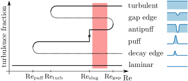
Figure 1: Sketch of the bifurcation diagram for transitional pipe flow. Attracting states are solid lines, unstable edge states are dotted. In the deterministic Barkley model used here $r_{\text{turb}}=0.667,r_{\text{slug}}=0.726,r_{\text{gap}}=0.736$

II A unified bifurcation diagram

We propose two novel states which complete the set of basic states in the transitional region, Fig. 1: the gap edge and antipuff. These are traveling wave states, consisting of localized laminar flow embedded within homogeneous turbulence. In the region $\text{Re}_{\text{turb}}<\text{Re}<\text{Re}_{\text{slug}}$ the gap edge is an unstable state lying at the edge between sustained homogeneous turbulence and localized turbulence in the form of a puff, analogously to the decay edge separating the base laminar flow and the puff. Above $\text{Re}_{\text{slug}}$ puffs disappear but the gap edge remains, separating homogeneous turbulence from a stable laminar pocket state we call an antipuff, which is the mirror image of a puff. Note that at $\text{Re}_{\text{slug}}$, slugs neither expand nor contract, corresponding to multiple solutions with sections of arbitrary length at the turbulent and laminar fixed points, which can be interpreted either as puffs or antipuffs, represented by a vertical line in Fig. 1. Finally, the gap edge and the antipuff disappear together at $\text{Re}_{\text{gap}}$. We propose that the intermittent turbulence regime observed in pipe flow corresponds to the random excitations and decays of antipuffs through the decay edge, and thus $\text{Re}_{\text{gap}}$ marks the end of this regime. A connection of the observed laminar pockets, here interpreted as antipuffs, to the laminar tails of slugs has been previously recognized Moxey and Barkley (2010); Barkley (2016), though their existence as distinct stable structures not explicitly stated. We now substantiate this picture and flesh out the conditions for its validity.

II.1 General considerations

A key characteristic of puffs are fronts: spatial locations where, while $u$ remains roughly constant, the turbulence level, $q$, either sharply rises from zero to a finite value (the upstream front with $u=U_{0}$) or sharply decreases to zero from a finite value (downstream, with $u<U_{0}$). The front speeds determine the speed of puffs and the Re range for their existence. Analogously, front speeds play a key role in establishing the existence of antipuffs. We denote by $c_{+}(u,\text{Re})$ ($c_{-}(u,\text{Re})$) the front speed at mean velocity $u$ where the turbulence level increases (decreases) in the downstream direction. Turbulence has been shown to be advected with speed $u-\zeta$ in pipe flow Song et al. (2017), where $\zeta$ is a constant offset velocity from the centerline value. Writing $c_{-}(u,\text{Re})=u-\zeta+S(u,\text{Re})$, the relative speed $S(u,\text{Re})$ thus determines the relative stability of laminar flow ($q=0$) compared with a turbulent flow ($q\neq 0$) at a common velocity $u$. Indeed, if $S(u,\text{Re})<0$ the downstream laminar flow overtakes the upstream turbulent flow, which is thus less stable at this $u$ Pomeau (1986). As $c_{+}(u,\text{Re})$ represents the same physics but with turbulence downstream of laminar flow, $c_{+}(u,\text{Re})=u-\zeta-S(u,\text{Re})$ . Puffs exist as long as front speeds match: there exists $u_{p}$ such that $c_{-}(u_{p},\text{Re})=c_{+}(U_{0},\text{Re})$. At $\text{Re}>\text{Re}_{\text{slug}}$, $u_{p}<u_{t}$, where $u_{t}$ is the homogeneous turbulence mean flow. Puffs are replaced by weak slugs, which have a downstream front at the turbulent velocity $u_{t}$. Since $c_{-}(u_{t},\text{Re})>c_{+}(U_{0},\text{Re})$ slugs expand. Generally, $S(u,\text{Re})$ is an increasing function of $u$ and Re: the higher the shear, the higher the production of turbulence; the higher the Re the lower the dissipation of turbulence—both making turbulence more sustainable.

The condition for existence of antipuffs is a region where $S(u_{t},\text{Re})<0$ for $\text{Re}>\text{Re}_{\text{slug}}$, satisfied in pipe flows for $\text{Re}\in(2250,3000)$ Song et al. (2017). Indeed, starting from a fully turbulent pipe flow, $q=q_{t},u=u_{t}$, imagine a local decrease of the level of turbulence to zero in a small interval in the pipe, while keeping $u=u_{t}$. This forms two fronts back to back, with relative speed $c_{+}(u_{t},\text{Re})-c_{-}(u_{t},\text{Re})=-2S(u_{t},\text{Re})>0$ producing an initially expanding laminar region. The flat turbulent profile, however, cannot be sustained at $q=0$, and $u$ will relax towards $U_{0}$. If $u$ were to reach $U_{0}$, forming an upstream front of a slug, then the gap would tend to close since $c_{+}(u_{t},\text{Re})-c_{-}(U_{0},\text{Re})<0$. Thus, there exists a velocity $u_{t}<u_{\text{ap}}<U_{0}$, the antipuff speed, giving matching front speeds $c_{-}(u_{t},\text{Re})=c_{+}(u_{\text{ap}},\text{Re})$ which define the antipuff. At $\text{Re}=\text{Re}_{\text{slug}}$ puff fronts satisfy $c_{-}(u_{t},\text{Re}_{\text{slug}})=c_{+}(U_{0},\text{Re}_{\text{slug}})$, so that $u_{\text{ap}}=U_{0}$ is a solution for antipuff fronts. Assuming it is unique, then $\text{Re}<\text{Re}_{\text{slug}}$ gives $u_{\text{ap}}>U_{0}$ and antipuffs disappear. At the other end, antipuffs merge with the gap edge and disappear once $S(u_{t},\text{Re})=0$, occurring at $\text{Re}=\text{Re}_{\text{gap}}$. To motivate the existence and structure of the gap edge, consider reducing $q$ locally in a turbulent pipe keeping $u=u_{t}$: the level of turbulence will return to $q_{t}$ if reduced by a minuscule amount, homogeneous turbulence being stable, while setting $q=0$ will open a laminar pocket which will expand into an antipuff (or puff, depending on Re). Thus, there exists an intermediate value of turbulence $0<q_{g}<q_{t}$ right at the boundary, allowing for a traveling wave solution with upstream $q_{t}\to q_{g}$, and downstream $q_{g}\to q_{t}$ fronts at almost the same speed $u\approx u_{t}$ (due to slow adjustment of $u$ to $q$), traveling at speed close to $u_{t}-\zeta$.

III The Barkley model

We now turn to the Barkley model, describing the numerical results we have obtained in support of the above described picture, as well as some asymptotic analytical results. The dynamics in the Barkley model reads

$$\begin{cases}\partial_{t}q+(u-\zeta)\partial_{x}q=f_{r}(q,u)+D\partial_{x}^{2}q+\sigma q\eta\\ \partial_{t}u+u\partial_{x}u=\epsilon\left[(U_{0}-u)+\kappa(\bar{U}-u)q\right]\\ \end{cases}$$ (1)

with $f_{r}(q,u)=q(r+u-U_{0}-(r+\delta)(q-1)^{2})$. Velocities are normalized such that $\bar{U}=1$ and $U_{0}=2$. The parameter $r$ plays the role of Re and $\eta$ is a spatiotemporal white noise with strength $\sigma$, modeling chaotic fluctuations. While the real turbulent states are chaotic and spatially intricate, the essential dynamical and physical features in the transitional region are very well captured within the Barkley model Barkley et al. (2015); Barkley (2016).

III.1 Results for the Barkley model

We first present the new states, obtained numerically for the model and then provide the details for the numerical methodology. The spatial profile of an antipuff as well as that of the gap edge, the latter obtained by edge tracking, are shown in Fig. 2 for a representative value of $r$. Note that while the turbulence drops to zero inside the antipuff, the centerline velocity $u$ does not reach the laminar value of $2$, consistent with observations in pipe flow Moxey and Barkley (2010).

The full bifurcation diagram is shown in Fig. 3, where states are ordered by their turbulent mass. The measured bifurcations for the Barkley model are exactly those sketched in Fig. 1. Note the gap in turbulent mass formed between the turbulent state and the gap edge with increasing $r$, and the eventual merging of the gap edge and antipuff as expected.

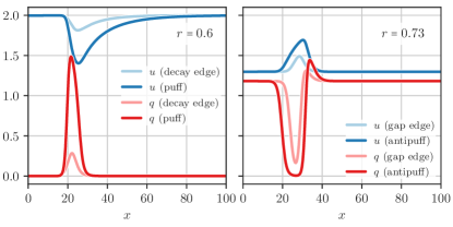
Figure 2: Spatial profiles of turbulence level $q$ and mean velocity $u$ in the Barkley model: puff and decay edge at $r<r_{\text{turb}}$ (left), and antipuff and gap edge at $r_{\text{slug}}<r<r_{\text{gap}}$ (right).

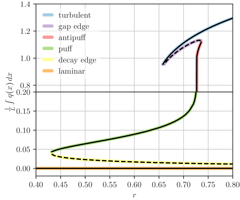
Figure 3: Explicitly computed bifurcation diagram for the Barkley model. The stable states for each $r$ (laminar, turbulent, puff, antipuff) are computed by relaxation of the dynamics. The unstable edge states (gap edge, decay edge) are computed by the edge tracking algorithm described in section III.2.2. Note the jump in the $y$-axis from 0.2 to 0.8 at the solid horizontal grid line.

III.2 Methodology for numerical experiments

For the numerical experiments using the Barkley model (1), we use the same parameters as in Ref. Barkley (2016): $\zeta=0.8$, $\delta=0.1$, $\varepsilon_{1}=0.1$, $\varepsilon_{2}=0.2$, $U_{0}=2$, $\bar{U}=1$, $D=0.5$, and $x\in[0,L]$ periodic with $L=100$. Space is discretized with $N_{x}=128$ or $N_{x}=256$ grid points, and spatial derivatives are computed via fast Fourier transforms. Temporal integration is performed by a first-order exponential time differencing (ETD) scheme Cox and Matthews (2002), with time-steps between $\Delta t=10^{-2}$ and $\Delta t=10^{-3}$. In simulations including stochastic noise, we use a noise-strength $\sigma=0.2$, and include the stochastic term by generalizing ETD to the stochastic integral, similar to Kloeden et al. (2011); Lord and Tambue (2013).

III.2.1 Projection onto non-moving reference frame

All spatially non-trivial attracting states we will be focusing on for the deterministic Barkley model are so-called relative fixed points—they are traveling wave solutions which move with a constant speed along the pipe. In the reference frame moving with this velocity they turn into fixed points, and in a periodic domain such as ours, they are limit cycles in the lab reference frame. In order to find these solutions with classical algorithms designed to obtain temporally constant configurations, we project the equations adaptively in time onto the corresponding moving reference frame, the idea is similar to that developed in Del Alamo and Jimenez (2009); Kreilos et al. (2014).

In particular, in order to adaptively eliminate the object’s translation along the pipe, we project the deterministic drift of the equation onto its part perpendicular to translation. This can be done by realizing that $\partial_{x}$ is the generator of translations, so that $n=\partial_{x}(q,u)$ is the direction in configuration space at the point $(q,u)$ that points into the direction of spatial translation. We can then project the right-hand-side of the deterministic part of equation (1),

$$\partial_{t}(q,u)=b(q,u)=(b_{q}(q,u),b_{u}(q,u))$$ (2)

with

$$\begin{cases}b_{q}(q,u)=f(q,u)+D\partial_{x}^{2}q+(\zeta-u)\partial_{x}q\\ b_{u}(q,u)=g(q,u)+D_{u}\partial_{x}^{2}u-u\partial_{x}u\\ \end{cases}$$ (3)

onto the subspace orthogonal to $n$,

$$\tilde{b}=b-\frac{n}{|n|^{2}}\langle n,b\rangle\,,$$ (4)

where $|.|$ and $\langle.,.\rangle$ are $L^{2}$ norm and inner product, so that the $\tilde{b}$-dynamics have no translational component. This allows us to obtain dynamics

$$\partial_{t}(q,u)=\tilde{b}(q,u)\,,$$ (5)

that only model the deformation of objects but not their movement speed. Note additionally that the prefactor of this projection will yield the movement speed of the object,

$$v(q,u)=\frac{\langle n,b\rangle}{|n|^{2}}\,,$$ (6)

since

$$\partial_{t}(q,u)=\tilde{b}(q,u)+v(q,u)\partial_{x}(q,u)\,.$$ (7)

In these projected dynamics, all states we are interested in (puff, antipuff, decay edge, gap edge) are fixed points of the $\tilde{b}$ dynamics, with $\tilde{b}=0$. For example, the decay edge which is a limit cycle of $b$ is now a fixed point with $\tilde{b}=0$, and has a single unstable direction corresponding to either decaying into the laminar state, or being the minimal seed to form a puff.

Not only does this procedure allow us to treat the configurations of interest as proper fixed points, but it also eliminates any CFL condition from the advective term. In combination with the usage of ETD this means that the reaction terms ($f(q,u)$ and $g(q,u)$) are the only terms restricting the time step.

Note that we use this projection only for our deterministic computations, as the interaction of the (spatially very rough) random noise with the spatial derivative needed to compute the translational component makes the projection inaccurate. For stochastic simulations, we instead apply a spatial translation at each iteration so that that the center of turbulent mass, $\langle x\rangle_{q}=\int_{0}^{L}x\,q(x)\,dx/\int_{0}^{L}q(x)\,dx$ remains at the domain center.

III.2.2 Edge tracking algorithm

In order to find the stable deterministic fixed points of the Barkley mode, it is enough to run numerical simulations until convergence, starting from an appropriate initial condition. For example, in order to generate the stable puff state, we initialize with a localized region of turbulence, which turns out to be a configuration within the basin of attraction of the puff state for properly chosen $r$.

For finding the unstable fixed points, in particular the relevant edge states between puff and laminar flow (the decay edge), and between turbulent flow and puff or antipuff (the gap edge), we employ edge tracking. The algorithm is implemented as follows: Define by $B(q,u)$ the map from a configuration $(q,u)$ to its basin of attraction $B\in\{\text{laminar},\text{puff},\text{turbulent},\text{antipuff},\text{two puffs},\ldots\}$. Numerically, we implement this function by integrating the deterministic dynamics until they are stationary, and comparing their turbulent mass $\bar{q}=\int_{0}^{L}q(x)\,dx$ with that of the known fixed points. While in general this comparison would be inconclusive (for example, a slug might have the same turbulent mass as two puffs), it is sufficient to identify the fixed points once the configuration is fully converged and no longer changes.

Now, to obtain the deterministic edge state, we then integrate two separate configurations of the system, $z_{0}=(q_{0},u_{0})$ and $z_{1}=(q_{1},u_{1})$, initialized to the two fixed points between which we want to find the edge state, for example $B(z_{0})=\text{laminar}$ and $B(z_{1})=\text{puff}$. Via bisection, we iteratively approach the basin boundary until the distance $d$ between $z_{0}$ and $z_{1}$ is below some threshold, $d(z_{0},z_{1})<\Delta_{\text{min}}$, making sure that we also retain that $B(z_{0})=\text{laminar}$ and $B(z_{1})=\text{puff}$. Since the basin boundary is generally repulsive, $z_{0}$ and $z_{1}$ will over time separate. Whenever they have separated too much, $d(z_{0},z_{1})>\Delta_{\text{max}}$, we perform another bisection procedure until they are again close together. This procedure is performed until the states $z_{0}$ and $z_{1}$ converge. Effectively, the algorithm integrates the dynamics restricted to the separating sub-manifold, by restricting the dynamics in the unstable direction (the separation between $z_{0}$ and $z_{1}$), while not interfering with all other directions. The end result is a state which is stable when restricted to the separating manifold, which corresponds to a fixed point of the dynamics with a single unstable direction, precisely the “saddle points” or edge states we are interested in.

III.2.3 Bifurcation diagram for the Barkley model

With the edge tracking algorithm lined out above, the schematic bifurcation diagram shown in figure 1 can be computed explicitly for the Barkley model by computing the relevant fixed points and edge states for each value of $r$.

In order to efficiently compute edge states, in particular the gap edge in the puff regime, we employed two additional techniques: First, we used continuation to get a good first guess for the gap edge at a given $r$ by using the previous result for the edge computation at a close-by $r$. Second, close to the edge we can use a local-in-time heuristic to decide on which side of the basin boundary a configuration is located: If its turbulent mass $\bar{q}$ is increasing in time, the configuration lies towards the turbulent fixed point, while if $\bar{q}$ is decreasing in time, the configuration lies towards the puff (or antipuff). While this criterion is only true close to the edge, it allows us to compute the unstable branch much more efficiently.

III.3 Asymptotic results for the Barkley model

Here we demonstrate how the general arguments made above manifest themselves in the deterministic Barkley model using analytical arguments. We will focus on leading order results in $\epsilon\ll 1$, which is the parameter controlling the slow relaxation of the mean shear $u$ in the model.

Above we have denoted front speeds by $c_{\pm}(u,r)=u-\zeta\mp S(u,r)$, while in the notations of Barkley (2016) $S(u,r)=\sqrt{D}s(u,r)$. Using standard techniques Keener and Sneyd (2009); Engel et al. (2021), it can be shown that at leading order in $\epsilon$

$$s(u,r)=3\sqrt{\frac{r+u-U_{0}}{2}}-\sqrt{\frac{r+\delta}{2}}.$$ (8)

One can then solve explicitly for the velocity $u_{p}$ at the downstream front of a puff, though that gives a lengthy expression which we omit here. The turbulent fixed point $(q_{t},u_{t})$ corresponds to the intersection of the $u$ nullcline with the $q$ (upper branch) nullcline defined by $q_{+}=1+\sqrt{\frac{r+u-U_{0}}{r+\delta}}$, $u_{t}$ being the solution to the equation $U_{0}-u+\kappa(\bar{U}-u)q_{+}(u,r)=0$. The turbulent fixed point first appears at $r_{\text{turb}}$, at the intersection of the $u$ nullcline with the nose of the $q$ nullcline which is at $q_{t}=1$. This gives

$$u_{t}(r_{\text{turb}})=\frac{(U_{0}+\kappa\bar{U})}{1+\kappa}$$ (9)

and

$$r_{\text{turb}}=\frac{\kappa(U_{0}-\bar{U})}{1+\kappa}$$ (10)

with $r_{\text{turb}}=2/3$ for our parameters.

III.3.1 The gap edge

We now discuss the gap edge in the limit $\epsilon\to 0$. We note that many characteristics we describe below are identical to those of the decay edge in this limit. We build on the analysis presented in Barkley (2016) to make our arguments for the properties of the gap edge.

To solve for the structure of the gap edge in the limit $\epsilon\to 0$, we may consider $u=u_{t}$ fixed and solve for $q$ at this fixed $u$ (this is also true for fronts of puffs and antipuffs). Then, assuming a traveling wave solution at speed $c_{g}$, and moving into its reference frame, the dynamical equation for $q$ becomes a spatial ODE:

$$D\partial_{xx}q=-(c_{g}-u_{t}+\zeta)\partial_{x}q-f(q,u_{t})$$ (11)

This is equivalent to a particle with position $q$, moving in a force field $-f(q,u)$ with linear friction with coefficient $c_{g}-u_{t}+\zeta$ acting on it. The system being one dimensional, the force can be written as a derivative of an (inverted) potential $V_{r}(q)$, with $f(q,u)=\partial_{q}V_{r}(q)$, which has maxima at $q=0$ and $q=q_{+}(r,u_{t})$. This is an inverted potential compared to the local dynamics for $q$, i.e $\partial_{t}q$ keeping $u$ fixed and considering a spatially homogeneous solution.

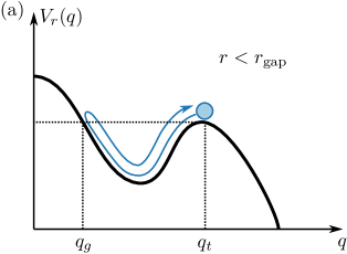
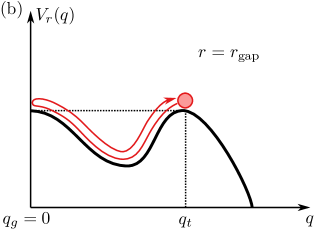
Figure 4: (a): The spatial structure of the gap edge $q(x)$ corresponds to a homoclinic trajectory of a particle moving in the potential $V_{r}(q)$, with $\partial_{q}V_{r}(q)=f(q,u)$ and $x$ playing the role of time. The particle starts at $q_{t}$, reaches $q_{g}$ and returns. (b) When $r=r_{\text{gap}}$, this homoclinic trajectory goes all the way to $q_{g}=0$.

The gap edge solution corresponds to a homoclinic trajectory of the one particle system 11: going from $q_{t}$ and back, i.e $q(x\to\pm\infty)=q_{t}$ with zero ”velocity” $\dot{q}(x\to\pm\infty)=0$. Such a trajectory is possible as long as $q=q_{t}$ is the lower maximum of the potential compared to $q=0$, which in terms of the local dynamics of $q$ corresponds to turbulent flow being a local minimum of the potential while laminar flow is a global minimum. From conservation of energy in the one particle system (or time reversal symmetry where $x$ plays the role of time), such a trajectory requires zero friction (meaning conservative one particle dynamics), giving $c_{g}=u_{t}-\zeta$. For $r<r_{\text{gap}}$, this situation is depicted in figure 4 (a). As $r$ increases, the turbulent fixed point becomes more stable: it rises in relative height in the inverted potential, making the homoclinic trajectory approach closer to $q=0$ as the (potential) energy of the initial condition increases, until the laminar and turbulent maxima have identical height. At this $r=r_{\text{gap}}$, the trajectory goes all the way to $q=0$ and the homoclinic orbit is made of two heteroclinic orbits connecting the two fixed points. This is the point where the gap edge and antipuff merge, the fronts of the gap edge becoming fronts of antipuffs which go all the way to/from $q=0$, as depicted in figure 4 (b). The corresponding mathematical details are more thoroughly discussed in a general context in Barkley (2016) Appendix A.

III.3.2 The antipuff regime

The transition from puffs to slugs happens when $u_{t}(r)=u_{p}(r)$, which for our parameters gives $r_{\text{slug}}\approx 0.76$, though $O(\epsilon)$ corrections are significant here since the range $r_{\text{slug}}-r_{\text{turb}}$ is itself of this order. At this $r=r_{\text{slug}}$, $S(u_{t},r)=-0.13$, i.e negative as required for the existence of an antipuff. Furthermore, solving numerically for $u_{t}$ we obtain that $S(u_{t}(r),r\approx 0.83)=0$ so that $r_{\text{gap}}\approx 0.83$ (again $\epsilon$ corrections are significant here). Note that $r=r_{\text{gap}}$ is not necessarily the point where weak fronts of the slug  stop existing, which instead requires $-\zeta+S(u_{t},r)>0$ Barkley (2016); Song et al. (2017).

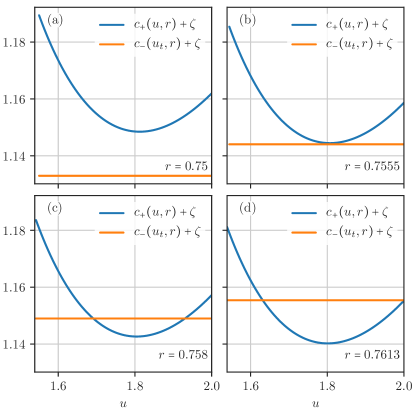
Figure 5: Matching between upstream and downstream speeds for antipuffs in the asymptotic Barkley model. (a) Below $r=0.75$ there is no solution for $u_{\text{ap}}$. (b) At $r\approx 0.7555$ there is a single solution, $u_{\text{ap}}\approx 1.8$ (c) For $0.7555\lesssim r\lesssim 0.7613$ there are two solutions. (d) At $r\approx 0.7613$ the higher velocity solution occurs at $u_{\text{ap}}=U_{0}=2$, corresponding to the identification between the downstream front of a puff and that of the unstable antipuff.

Although above we have focused on the case of a unique solution for $u_{\text{ap}}$, here in the limit of $\epsilon\to 0$ there are in fact two possible solutions. A match between front speeds of the antipuff is first possible at $r_{\text{ap}}\approx 0.756<r_{\text{slug}}\approx 0.76$ giving $u_{\text{ap}}\approx 1.8$ (for this $r$, $u_{t}\approx 1.29$). In particular, at $r_{\text{ap}}\approx 0.756$ the minimum of the curve $c_{+}(u,r)=u-\zeta-S(u,r)$, given by $u=U_{0}-r-\frac{9D}{8}\approx 1.8$ touches the line $c_{-}(u_{t},r)$, see Fig. 5(a,b). This corresponds to the appearance of one stable and one unstable antipuff in a saddle node bifurcation, as discussed below. Indeed, at higher $0.756<r<r_{\text{slug}}$ there are two intersection points between $c_{+}(u,r)=u-\zeta-S(u,r)$ and the line $c_{-}(u_{t}(r),r)$ inside the segment $u_{t}(r)<u<U_{0}$, giving two solutions for $u_{\text{ap}}$ as in Fig. 5(c). At $r=r_{\text{slug}}\approx 0.76$ the larger of the two velocities satisfies $u_{\text{ap}}=U_{0}=2$ so that its downstream front is identical to that of a puff, see Fig. 5(d). We will discuss how this two antipuff scenario will manifest itself in the bifurcation diagram in the next section. However, while it is probably realized in the Barkley model for very small but finite $\epsilon$, its region of existence in $r$ is minuscule, $0.756<r<0.76$, making it indistinguishable in practice from a single antipuff appearing at $r_{\text{slug}}$. Thus, we could not satisfactorily verify it in numerical simulations.

IV Alternative scenarios for the bifurcation diagram

Here we consider two alternative scenarios to the bifurcation diagram presented in Fig. 1. Remarkably, in these scenarios there is a range of Re for which puffs and antipuffs coexist. Both scenarios appear to be inconsistent with observations for pipe flow, though the differences are subtle and thus could be relevant to other wall bounded flows where puff-like and slug-like structures occur.

The three main assumptions we have made so far are: (i) a continuous transition from puffs to slugs, implying $\text{Re}_{\text{turb}}<\text{Re}_{\text{slug}}$, (ii) at $\text{Re}_{\text{slug}}$ homogeneous turbulence is metastable compared to laminar flow, corresponding to $S(u_{t},\text{Re}_{\text{slug}})<0$ as can be measured at the downstream front of a slug, and (iii) there is a unique solution for the antipuff speed $u_{\text{ap}}$ which gives fronts of matching speed. While the first two assumptions can be directly measured, the third assumption is more subtle but could still be checked: it implies that a puff continuously turns into an antipuff when viewed in the q-u plane. That indeed appears to be the case for pipe flow Moxey and Barkley (2010), though this issue has not be at the focus of a dedicated study. In the following we will assume (i) is satisfied throughout, though we are not aware of a general argument precluding a discontinuous transition from puffs to slugs.

We begin by exploring the consequences of breaking assumption (iii) while keeping (i) and (ii). Indeed, the equation determining the speed of the downstream front of an antipuff does not necessarily have a unique solution: $u_{\text{ap}}-S(u_{\text{ap}},\text{Re})=u_{t}+S(u_{t},\text{Re})$ can have more than one solution, but at most two, since $S(u_{\text{ap}},\text{Re})$ is an increasing function of $u_{\text{ap}}$. Thus the right hand side of the equation is not necessarily monotonic but at most has one extremum. If there are indeed two solutions for $u_{\text{ap}}$, they correspond to the presence of a stable and an unstable antipuff, and we will denote by $\text{Re}_{\text{ap}}$ the Reynolds number where they first appear together. Note that $\text{Re}_{\text{ap}}>\text{Re}_{\text{turb}}$ since an antipuff is a localized state within homogeneous turbulence. For $\text{\text{Re}}_{\text{ap}}<\text{Re}<\text{\text{Re}}_{\text{gap}}$, creating a laminar pocket within homogeneous turbulence will lead to the formation of an antipuff. Thus, the gap edge lies at the boundary between turbulence and the stable antipuff state and the bifurcation diagram is unchanged for $\text{Re}_{\text{slug}}<\text{Re}<\text{Re}_{\text{gap}}$. Like before, $\text{Re}_{\text{gap}}$ corresponds to the point where the gap edge merges with an antipuff.

The stable antipuff appears at $\text{Re}_{\text{ap}}$ and disappears at $\text{Re}_{\text{gap}}$. Thus, the unstable antipuff must disappear at $\text{Re}_{\text{slug}}$. Indeed, at $\text{Re}_{\text{slug}}$ $u_{\text{ap}}=U_{0}$ is a solution, since a slug has matching upstream and downstream front speeds at this Re. Thus, like previously, a puff turns into an antipuff at $\text{Re}_{\text{slug}}$, but here it is the unstable antipuff. Note that slugs, which connect the laminar base flow with homogeneous turbulence, are still contracting (since $u_{p}>u_{t}$) for all $\text{Re}_{\text{turb}}<\text{Re}<\text{Re}_{\text{slug}}$. However, even though slugs are contracting, if one were to sufficiently decrease the mean flow in the laminar region, then the laminar region would contract to a finite length, forming the stable antipuff. The corresponding bifurcation diagram is presented in Fig. 6 (a).

As a second alternative, let us briefly discuss the case where assumption (ii) is broken while keeping assumption (i). This corresponds to assuming $S(u_{t},\text{Re}_{\text{slug}})>0$, but that puffs still continuously turn into slugs at $\text{Re}_{\text{slug}}$. In particular, the condition $S(u_{t},\text{Re}_{\text{slug}})<\zeta$ for the existence of a weak slug front is assumed to still be satisfied Barkley (2016). In this case, $\text{Re}_{\text{gap}}<\text{Re}_{\text{slug}}$ so that stable antipuffs disappear before $\text{Re}_{\text{slug}}$. It follows that this is also a regime with two antipuffs, breaking also assumption (iii), the unstable antipuff disappearing at $\text{Re}_{\text{slug}}$ as before. No intermittent turbulent regime can exist in this case. This scenario is sketched in Fig. 6 (b).

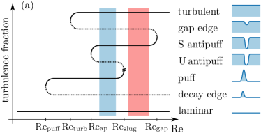
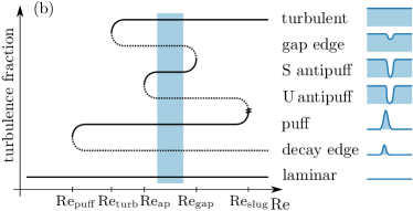
Figure 6: Alternative bifurcation diagrams for transitional flow. (a): Existence of two antipuff solutions, with the unstable (“U antipuff”) and stable antipuff (“S antipuff”) being created out of a saddle-node bifurcation at $\mathrm{\text{Re}}_{\text{ap}}$. Note the co-existence of puffs and antipuffs in this regime. The intermittent turbulence regime is marked in red. (b) Disappearance of the gap edge before the transition to slugs: $\mathrm{\text{Re}}_{\text{gap}}<\mathrm{\text{Re}}_{\text{slug}}$. Like in (a) there are two antipuff solutions and a coexistence region between antipuffs and puffs. The intermittent turbulence regime is absent.

V Intermittent turbulence regime

As stated above, we propose that the intermittent turbulence regime corresponds to the range $\text{Re}_{\text{slug}}<\text{Re}<\text{Re}_{\text{gap}}$, so that laminar pockets within homogeneous turbulence observed in simulations of pipes Moxey and Barkley (2010) are in fact antipuffs which are excited and subsequently decay. Both excitations and decays are expected to occur through the gap edge. These laminar pockets set the fraction of laminar flow within homogeneous turbulence, and thus have a similar role to that of puffs for the reverse transition from turbulence to laminar flow. Antipuffs however do not completely mirror puffs: they can be spontaneously excited from the turbulent state, as it is not absorbing, while on the other hand they cannot split. The fraction of laminar flow in the homogeneous turbulent state is thus controlled by the probabilities of antipuff excitations and decays. These vary smoothly with Re, excitations becoming rarer and lifetimes becoming shorter as the gap edge grows deeper, as indeed observed in pipe flow Moxey and Barkley (2010), and the Barkley model Barkley (2016). Thus, this is not a phase transition and in particular there is no critical point corresponding to it.

We now wish to demonstrate that the laminar pockets within homogeneous turbulence observed in the Barkley model indeed correspond to the excitations and decays of antipuffs. We therefore consider the stochastic Barkley model. The stochastic model had been previously explored for the noise level $\sigma=0.5$ in  Barkley (2016), but this level of noise is so high that laminar flashes are frequent. Thus, the observation of a single creation and decay event is hard, the pockets lifetimes are short, and multiple laminar pockets regularly coexist. In order to isolate creation and decay of a single stochastic laminar pocket, we perform numerical simulations at a lower noise level, $\sigma=0.22$ and in Fig. 7 present a stochastic creation event (left panel), and a stochastic decay event (right panel) both at $r=0.748$ which is lower than $r_{\text{gap}}$ for this noise level.

In addition, we show the profile of the stochastic laminar pocket in Fig. 8, where we present both the spatial $q$ and $u$ profile for an average pocket (right) and a $q$-$u$-plot (left), which includes both the average as well as the density of individual realizations. The averaging is performed by aligning the structures in space according to the downstream front, which is therefore sharp. Note that this smears the upstream front making the average less representative, as is evident in the $q$-$u$-plot, since the spatial extent of the pocket tends to vary significantly, as seen in Fig. 7. The resemblance of the average structure to the deterministic antipuff is striking. It is also evident, for the mean as well as for individual realizations, that the mean shear $u$ never reaches the laminar value $U_{0}=2$, a characteristic feature of antipuffs.

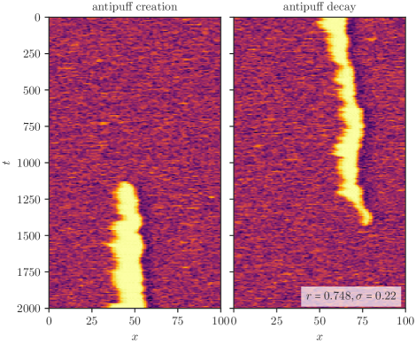
Figure 7: For $r=0.748$, $\sigma=0.22$, the antipuff is long lived, but noise is strong enough to drive a rare transition from turbulent flow into the antipuff (left), and from an antipuff back into the fully turbulent flow (right).

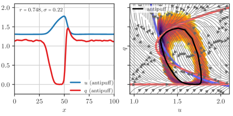
Figure 8: Spatial structure (left) and $q$-$u$-plot (right) of the antipuff at $r=0.748$, $\sigma=0.22$. Many realizations of the stochastic antipuff are aligned at the downstream front to obtain its average form. In the $q$-$u$-plane, we superimpose a density plot of all considered realizations of the antipuff.

VI Conclusion

We have motivated the existence of two novel states: the gap edge and the antipuff and have discussed how they fit within a bifurcation diagram involving previously known states. Our work motivates the study of antipuffs as well defined separate states, as well as a search for the gap edge. It further suggests the existence of invariant solutions which have a localized laminar region (e.g. where streamwise vorticity is depleted) embedded in a turbulent (vortical) flow, as those could be underlying the gap edge and the antipuff state.

Taken together, a unified dynamical picture of the transitional regime emerges: laminar gaps forming within homogeneous turbulence are the mirror images of turbulent patches embedded within laminar flow. Still, the transition from laminar flow to turbulence with increasing Re is not the mirror image of the transition from homogeneous turbulence to laminar flow with decreasing Re. This is a consequence of the absorbing nature of the laminar base flow, which the homogeneous turbulent state does not share. Thus, while the former transition is a proper phase transition, the latter is not.

Finally, while we believe the bifurcation diagram we presented is relevant for pipe flow, other alternatives are also possible. We have presented two such alternatives here. In future work, it will be interesting to explore their possible relevance to other wall bounded flows and the ensuing consequences for the transition to and from turbulence.

Acknowledgments We are grateful to Dwight Barkley, Sébastien Gomé and Laurette Tuckerman for many helpful discussions and comments. We also thank Yariv Kafri, Dov Levine and Grisha Falkovich for discussions and comments on the manuscript. TG acknowledges the support received from the EPSRC projects EP/T011866/1 and EP/V013319/1.

References

- Reynolds (1883) O. Reynolds, Proc. R. Soc. 35 (1883), 10.1098/rspl.1883.0018.
- Lindgren (1957) E. R. Lindgren, Arkiv fysik 12 (1957).
- Wygnanski and Champagne (1973) I. J. Wygnanski and F. Champagne, Journal of Fluid Mechanics 59, 281 (1973).
- Manneville (2016) P. Manneville, Mechanical Engineering Reviews 3, 15 (2016).
- Avila et al. (2011) K. Avila, D. Moxey, A. de Lozar, M. Avila, D. Barkley, and B. Hof, Science 333, 192 (2011).
- Moxey and Barkley (2010) D. Moxey and D. Barkley, Proceedings of the National Academy of Sciences 107, 8091 (2010).
- Mellibovsky et al. (2009) F. Mellibovsky, A. Meseguer, T. M. Schneider, and B. Eckhardt, Phys. Rev. Lett. 103, 054502 (2009).
- Duguet et al. (2010) Y. Duguet, A. P. Willis, and R. R. Kerswell, Journal of Fluid Mechanics 663, 180–208 (2010).
- Barkley (2016) D. Barkley, Journal of Fluid Mechanics 803 (2016), 10.1017/jfm.2016.465.
- Eckhardt et al. (2007) B. Eckhardt, T. M. Schneider, B. Hof, and J. Westerweel, Annual Review of Fluid Mechanics 39, 447 (2007).
- Skufca et al. (2006) J. D. Skufca, J. A. Yorke, and B. Eckhardt, Phys. Rev. Lett. 96, 174101 (2006).
- Schneider et al. (2007) T. M. Schneider, B. Eckhardt, and J. A. Yorke, Phys. Rev. Lett. 99, 034502 (2007).
- Avila et al. (2013) M. Avila, F. Mellibovsky, N. Roland, and B. Hof, Phys. Rev. Lett. 110, 224502 (2013).
- Pomeau (2015) Y. Pomeau, Comptes Rendus Mécanique 343, 210 (2015).
- Faisst and Eckhardt (2003) H. Faisst and B. Eckhardt, Phys. Rev. Lett. 91, 224502 (2003).
- Kerswell (2005) R. R. Kerswell, Nonlinearity 18, R17 (2005).
- Gibson et al. (2008) J. F. Gibson, J. Halcrow, and P. Cvitanović, Journal of Fluid Mechanics 611, 107–130 (2008).
- Kawahara et al. (2012) G. Kawahara, M. Uhlmann, and L. van Veen, Annual Review of Fluid Mechanics 44, 203 (2012).
- Duguet et al. (2008a) Y. Duguet, A. P. Willis, and R. R. KerswellL, Journal of Fluid Mechanics 613, 255–274 (2008a).
- Duguet et al. (2008b) Y. Duguet, C. C. T. Pringle, and R. R. Kerswell, Physics of Fluids 20, 114102 (2008b).
- Willis et al. (2013) A. P. Willis, P. Cvitanović, and M. Avila, Journal of Fluid Mechanics 721, 514–540 (2013).
- Budanur et al. (2017) N. B. Budanur, K. Y. Short, M. Farazmand, A. P. Willis, and P. Cvitanović, Journal of Fluid Mechanics 833, 274–301 (2017).
- Barkley et al. (2015) D. Barkley, B. Song, V. Mukund, G. Lemoult, M. Avila, and B. Hof, Nature 526, 550 (2015).
- Song et al. (2017) B. Song, D. Barkley, B. Hof, and M. Avila, Journal of Fluid Mechanics 813, 1045 (2017).
- Pope (2000) S. B. Pope, Turbulent Flows (Cambridge University Press, 2000).
- Pomeau (1986) Y. Pomeau, Physica D: Nonlinear Phenomena 23, 3 (1986).
- Note (1) This is only roughly true: the mean velocity profile advecting the turbulence creates an a-symmetry between the two fronts, which a 1D model cannot capture.
- Cox and Matthews (2002) S. Cox and P. Matthews, Journal of Computational Physics 176, 430 (2002).
- Kloeden et al. (2011) P. E. Kloeden, G. J. Lord, A. Neuenkirch, and T. Shardlow, Journal of Computational and Applied Mathematics 235, 1245 (2011).
- Lord and Tambue (2013) G. J. Lord and A. Tambue, IMA Journal of Numerical Analysis 33, 515 (2013).
- Del Alamo and Jimenez (2009) J. C. Del Alamo and J. Jimenez, Journal of Fluid Mechanics 640, 5–26 (2009).
- Kreilos et al. (2014) T. Kreilos, S. Zammert, and B. Eckhardt, Journal of Fluid Mechanics 751, 685–697 (2014).
- Keener and Sneyd (2009) J. Keener and J. Sneyd, Mathematical physiology I: Cellular physiology (Springer, 2009).
- Engel et al. (2021) M. Engel, C. Kuehn, and B. de Rijk, arXiv:2108.09990 [physics] (2021).
- Note (2) Weak fronts of slugs are fronts followed by a refractory laminar tail, where the flow relaxes to the base laminar flow.