Two Heads are Better than One: Geometric-Latent Attention for Point Cloud Classification and Segmentation

Abstract

We present an innovative two-headed attention layer that combines geometric and latent features to segment a 3D scene into semantically meaningful subsets. Each head combines local and global information, using either the geometric or latent features, of a neighborhood of points and uses this information to learn better local relationships. This Geometric-Latent attention layer (Ge-Latto) is combined with a sub-sampling strategy to capture global features. Our method is invariant to permutation thanks to the use of shared-MLP layers, and it can also be used with point clouds with varying densities because the local attention layer does not depend on the neighbor order. Our proposal is simple yet robust, which allows it to achieve competitive results in the ShapeNetPart and ModelNet40 datasets, and the state-of-the-art when segmenting the complex dataset S3DIS, with 69.2% IoU on Area 5, and 89.7% overall accuracy using K-fold cross-validation on the 6 areas.

1 Introduction

Robotics, autonomous driving, and related areas rely heavily on information captured by 3D sensors like RGB-D cameras, stereo cameras, and LiDARs. This information provides to the agent (robots or cars) the 3D location of their surroundings, which can be processed and used in tasks like scene understanding, path planning, navigation, among others [Cuevas-Velasquez et al.(2018)Cuevas-Velasquez, Li, Tylecek, Saval-Calvo, and Fisher, Cuevas-Velasquez et al.(2020)Cuevas-Velasquez, Gallego, Tylecek, Hemming, Van Tuijl, Mencarelli, and Fisher, Strisciuglio et al.(2018)Strisciuglio, Tylecek, Blaich, Petkov, Biber, Hemming, van Henten, Sattler, Pollefeys, Gevers, et al.]. One of the most used approaches to detect objects in 3D space is point cloud segmentation. A point cloud is a set of points in 3D, usually unordered and sparse; some regions can be densely populated and others empty. This type of non-grid structured data is difficult to be used with convolution operators with the same efficiency as their 2D counterpart.

Various approaches have been proposed to handle such data. Some approaches project the 3D raw data into a regular structure (e.g. voxels) where 3D convolutions can be used [Zhou and Tuzel(2018), Meng et al.(2019)Meng, Gao, Lai, and Manocha, Riegler et al.(2017)Riegler, Osman Ulusoy, and Geiger, Wang et al.(2017)Wang, Liu, Guo, Sun, and Tong, Klokov and Lempitsky(2017), Shao et al.(2018)Shao, Yang, Weng, Hou, and Zhou]. Other approaches use multilayer perceptrons (MLP) to process point clouds directly [Qi et al.(2017a)Qi, Su, Mo, and Guibas, Qi et al.(2017b)Qi, Yi, Su, and Guibas, Thomas et al.(2019)Thomas, Qi, Deschaud, Marcotegui, Goulette, and Guibas]. A third approach is to project the points to an intermediate grid structure where 2D convolutions can be used [Lin et al.(2020)Lin, Yan, Huang, Du, Liu, Cui, and Han, Huang et al.(2019)Huang, Zhang, Yi, Funkhouser, Nießner, and Guibas, Yang et al.(2020)Yang, Liu, Pan, Liu, and Tong]. Lately, with the success of transformers and attention mechanisms in the area of natural language processing (NLP) [Vaswani et al.(2017)Vaswani, Shazeer, Parmar, Uszkoreit, Jones, Gomez, Kaiser, and Polosukhin], these methods are starting to be used for 3D point cloud problems [Guo et al.(2020)Guo, Cai, Liu, Mu, Martin, and Hu, Qiu et al.(2021)Qiu, Anwar, and Barnes].

This paper proposes a multi-head attention layer called Geometric-Latent Attention (Ge-Latto) to segment and label subsets of the point cloud. Ge-Latto is a two-headed local attention layer that evaluates a patch inside the point cloud and tries to find good relationships between the neighbor points. Unlike other works that combine all the features indiscriminately [Zhao et al.(2020)Zhao, Jia, and Koltun, Li et al.(2018b)Li, Bu, Sun, Wu, Di, and Chen], each attention head focuses on a specific type of feature. One head is in charge of finding good geometric relations and the other in finding relationships among the latent features of the network. Similar to [Lin et al.(2020)Lin, Yan, Huang, Du, Liu, Cui, and Han], we use an encoder-decoder network with residual connections. Each layer of the encoder sub-samples the input points, groups the points into neighborhoods, and uses our Ge-Latto layer to find local-spatial relationships from the latent and geometric features of neighbor points. The neighbors are found using radius neighborhoods instead of k-nearest-neighbors (kNN). The network increases this radius in each layer to increase the field of view and find relationships in bigger neighborhoods. In the decoder part, we up-sample the points using tri-linear interpolation. To ensure that in each sampled layer the network learns useful features, we add auxiliary losses similar to PSPNet [Zhao et al.(2017)Zhao, Shi, Qi, Wang, and Jia] and RetinaNet [Lin et al.(2017)Lin, Goyal, Girshick, He, and Dollár]. In other words, the network predicts the segmentation for each sample size as seen in Figure 1. Our approach is also invariant to permutation because all the layers are shared MLPs.

The main contributions of this paper are: a) A novel two-headed attention layer that is able to combine efficiently the geometric and latent information of unordered point clouds with variable densities for semantic segmentation and shape classification. b) A pyramid-based encoder-decoder architecture with multi-resolution outputs and auxiliary losses to leverage feature patterns at different resolutions. c) State of the art performance on the complex dataset S3DIS. Not only in the area 5, but also in the k-fold cross-validation overall accuracy, as well as competitive results in the ShapeNetPart and ModelNet40 datasets.

2 Related Work

Recent works focus on how to handle unordered 3D points and find spatial relationships between them to better segment a point cloud. This section briefly reviews these methods and groups them into 4 categories.

Volumetric-based methods. These methods quantize an unordered point cloud in a uniform structure like voxels. Some approaches use 3D convolutions to find local relationships between closer groups of points [Zhou and Tuzel(2018), Meng et al.(2019)Meng, Gao, Lai, and Manocha]. However, the amount of memory required to compute these convolutions makes them unfeasible to process a large number of points. Methods like OctNet [Riegler et al.(2017)Riegler, Osman Ulusoy, and Geiger] and O-CNN [Wang et al.(2017)Wang, Liu, Guo, Sun, and Tong] save computation time by using octrees to avoid processing empty spaces. [Klokov and Lempitsky(2017)] and [Shao et al.(2018)Shao, Yang, Weng, Hou, and Zhou] use Kd-tree and Hash structures instead. [Tang et al.(2020)Tang, Liu, Zhao, Lin, Lin, Wang, and Han] uses sparse 3D convolutions rather than efficient data structures. Although these implementations reduce the computation required to train a 3D CNN, quantizing the points comes with the cost of losing important fine-grained information.

Point-based networks. These are networks capable of using irregular point clouds without projecting or quantizing them into regular grids. Their main characteristic is the use of shared MLP layers, also known as point-wise or 1D convolutional layers. PointNet [Qi et al.(2017a)Qi, Su, Mo, and Guibas] is a milestone of this kind of network. This approach uses MLP layers as permutation-invariant functions to process each point of a point cloud individually, and a max-pooling layer to aggregate them. The performance of the network is limited because they do not consider local spatial relationships in the data. PointNet++ [Qi et al.(2017b)Qi, Yi, Su, and Guibas] addresses this issue by sampling the points, grouping them in clusters, and applying PointNet on the clusters. SO-Net [Li et al.(2018a)Li, Chen, and Lee] uses a similar hierarchical structure adding self-organizing maps (SOMs) to capture better local structures. Other approaches like PointConv [Wu et al.(2019)Wu, Qi, and Fuxin], PointCNN [Li et al.(2018b)Li, Bu, Sun, Wu, Di, and Chen] and KPConv [Thomas et al.(2019)Thomas, Qi, Deschaud, Marcotegui, Goulette, and Guibas] construct kernels based on the input coordinates to be used as convolution weights.

Projection-based approaches. Some works project local neighborhoods into tangent planes and process them with 2D convolutions. The tangent plane parameters can be found using point tangent estimation [Tatarchenko et al.(2018)Tatarchenko, Park, Koltun, and Zhou], or approximated [Lin et al.(2020)Lin, Yan, Huang, Du, Liu, Cui, and Han, Huang et al.(2019)Huang, Zhang, Yi, Funkhouser, Nießner, and Guibas, Yang et al.(2020)Yang, Liu, Pan, Liu, and Tong]. The downside of these approaches is that they lose the information of 1 dimension given that they project the points to a local 2D plane.

Self-attention and transformers. Self-attention and transformers have revolutionized the area of NLP [Vaswani et al.(2017)Vaswani, Shazeer, Parmar, Uszkoreit, Jones, Gomez, Kaiser, and Polosukhin, Shaw et al.(2018)Shaw, Uszkoreit, and Vaswani]. This has lead the 3D segmentation field to investigate these techniques [Guo et al.(2020)Guo, Cai, Liu, Mu, Martin, and Hu, Qiu et al.(2021)Qiu, Anwar, and Barnes, Zhao et al.(2020)Zhao, Jia, and Koltun]. In the point cloud domain, self-attention networks can be seen as an improvement of the MLP networks, where instead of capturing local relationships by using pooling layers or weighting the features of the neighbors using hard-coded scores [Liu et al.(2020)Liu, Hu, Cao, Zhang, and Tong], they learn these relationships through an attention layer which estimates a score function to weight the contribution of each neighbor. The self-attention architecture resembles the encoder part of the transformers. One of the attempts to apply transformers to point clouds is PCT [Guo et al.(2020)Guo, Cai, Liu, Mu, Martin, and Hu]. They replace the MLP layers from PointNet++ with transformer layers and the output feature of each layer is enriched with a discrete Laplacian operator. There are two differences between PCT and ours. The first one is that they aggregate the points inside a neighborhood by applying maxpooling. We use self-attention instead, which allows the information from all the neighbors to be passed, rather than only using the neighbor with the highest feature value. The second difference is that they use global attention and we use local attention. This means that their method attends to all points, while ours attends to a local cluster of points. In terms of computation, their memory requirements are quadratic $[N\times N]$ while ours is $[K\times N]$ where $N$ is the number of points and $K$ the number of neighbors in the local cluster. [Qiu et al.(2021)Qiu, Anwar, and Barnes] uses geometric features to add extra information to semantic features, and self-attention and maxpooling are used to do the local aggregation. The same operation is performed at different scales and the results are combined using another self-attention layer.

The goal of 3D point cloud segmentation is to find good local relationships. Most of the methods use pooling operations [Qi et al.(2017a)Qi, Su, Mo, and Guibas, Qiu et al.(2021)Qiu, Anwar, and Barnes] to extract the important features inside a patch. However, this loses some information about the neighbors because these operations either return the maximum or average value of a group of points. The neighborhood information can be preserved better by using an attention mechanism, which helps the network to learn how much each neighbor contributes to the local patch. Although there are approaches that use self-attention [Qi et al.(2017b)Qi, Yi, Su, and Guibas, Guo et al.(2020)Guo, Cai, Liu, Mu, Martin, and Hu, Qiu et al.(2021)Qiu, Anwar, and Barnes], the type of attention they use is scalar. The problem with scalar attention is that it uses the same learned score for all the feature channels of a neighbor point. Our network instead uses vector attention [Zhao et al.(2020)Zhao, Jia, and Koltun], which computes a score for each channel individually, bringing more flexibility to the layer. We extend this flexibility by introducing a two-headed self-attention layer, where one head focuses on geometric features and the other on semantic features. Even though there are works [Qiu et al.(2021)Qiu, Anwar, and Barnes, Lin et al.(2020)Lin, Yan, Huang, Du, Liu, Cui, and Han] that use geometric and latent features, they treat them indistinguishably, losing the individual contribution of each feature. Our method can also be considered as one of the closest implementations to transformers for point cloud segmentation because, unlike previous research, we adapted one of the key properties of transformers, which is the multi-head attention structure.

3 Proposed Method

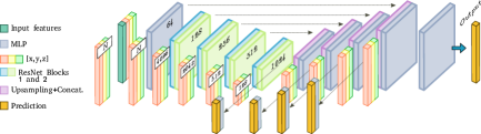
Figure 1: The encoder-decoder architecture receives as input $xyz$ coordinates and $RGB$. The figure shows the effect of the sub-sample process on the $xyz$ values and the output features of each encoder layer. The encoder consists of ResNet blocks, which have our Ge-Latto layer (see Figure 3). The decoder consists of up-sampling layers which are concatenated with their respective encoder features using residual connections and combined with an MLP.

Ge-Latto extracts two types of information from the point cloud: The geometric information obtained from the Cartesian coordinates of the points and the latent feature information learned by the network each time the point cloud is sub-sampled. The first part of this subsection describes the network architecture and sampling strategy. The second part describes the two-headed attention layer and explains how latent and geometric information is used.

3.1 Network and Sampling

The network has an encoder-decoder architecture and receives as input the $xyz$ coordinates and RGB color. Those features are projected to a higher dimension using a shared MLP layer (see Figure 1). The encoder reduces the number of points and extracts high-level features from a neighborhood of points. For this, each layer sub-samples the number of points of its input. Therefore $N_{l}>N_{l+1}$ where $N$ is the number of points and $l$ is the layer. The encoder has 4 layers that are designed like bottleneck ResNet blocks [He et al.(2016)He, Zhang, Ren, and Sun] with Ge-Latto replacing the 2D convolutions. Using Thomas et al[Thomas et al.(2019)Thomas, Qi, Deschaud, Marcotegui, Goulette, and Guibas] configuration, the input features of a ResNet block are processed by an MLP layer followed by batch normalization and ReLU. The other MLPs of the block are only followed by batch normalization (see Figure 3).

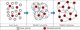
Figure 2: Clustering process inside ResNet blocks. The first image shows the input points of the layer. The grouping criteria of Block 1 and 2 are shown in the second and third image. Block 1 groups the input points using the sampled points as centers with a radius $r_{1}$, whereas Block 2 does the grouping on the sampled points with a bigger radius $r_{2}$.

Given the sparse nature of a point cloud, the choice of the sampling method is not trivial. The sampled points have to represent a group of points and be beneficial for the information “aggregation” of its neighbors. Here, we chose Farthest Point Sampling (FPS) because it outputs a more uniform-like distribution which is a desired property for point cloud semantic segmentation [Thomas et al.(2019)Thomas, Qi, Deschaud, Marcotegui, Goulette, and Guibas].

The next step groups each point $p_{i}$ from the input set $\mathcal{P}_{l}$ (of size $N_{l}$) with their neighbors to find local-spatial relationships. The points can be either grouped by kNN or radius neighbors. We use the latter because it is more robust with non-uniform sampling settings like point clouds [Thomas et al.(2019)Thomas, Qi, Deschaud, Marcotegui, Goulette, and Guibas]. Therefore, for each representative point $p_{i}\in\mathcal{P}_{l}$, $K$ points inside the given radius are randomly picked. We use $\mathcal{Q}_{i}$ to represent the grouped neighboring points of $p_{i}$ in the rest of the paper. It is important to note that $\mathcal{Q}_{i}\subseteq\mathcal{P}_{l-1}$, the only exception is in the second ResNet block, where $\mathcal{Q}_{i}\subseteq\mathcal{P}_{l}$ because no sampling is carried out; Figure 2 and Figure 3 show an example. The network also increases the receptive field by doubling the radius at every layer.

Figure 3: ResNet Blocks. The first block sub-samples the point cloud and finds nearest neighbors inside a radius between the sampled points and the input points. Because of the sampling, the residual connection has a maxpooling layer to match the input with the output size. The function of the second block is similar to the first one, but without sub-sampling.

For segmentation, the decoder up-samples the number of points until it recovers the size of the input of the network. The up-sampling of the features is done via tri-linear interpolation following Lin et al[Lin et al.(2020)Lin, Yan, Huang, Du, Liu, Cui, and Han]. The interpolated features are concatenated with the features from the corresponding encoder stage thanks to the residual connections (see Figure 1). The final and auxiliary outputs of the decoder are feature vectors for each point in the input point set. An MLP is used to map these features to the final logits, whose feature dimension is the number of classes. The size of the auxiliary outputs corresponds to the number of points their respective layers have. The network has 4 auxiliary outputs, one for the last encoder layer, and three for the following decoder layers. For classification, global average pooling is used over the last encoder features to get a global feature vector of the point cloud. This feature is passed to an MLP to obtain the classification logits.

3.2 Two-headed Attention

Figure 4: The two-headed Ge-Latto layer computes the local-attention for the geometric and latent features individually and then combines them using $f_{i}$ MLP layers.

We claim that our two-headed attention layer finds better features by combining geometric and latent information in each layer of the encoder (Figure 4). The geometric features that are used are the absolute position of the representative points $p_{i}\in\mathbb{R}^{3}$, the $K$ neighbor points $\mathcal{Q}_{i}\in\mathbb{R}^{K\times 3}$, and the relative position of the neighbors $\mathcal{Q}_{i}-\mathcal{K}p_{i}\in\mathbb{R}^{K\times 3}$, where the operator $\mathcal{K}$ replicates the vector K times. The latent information are the features learned by the hidden layers of the network. Each Ge-Latto layer uses those that belong to each centroid or representative point $r_{i}\in\mathbb{R}^{D}$, the features of the neighbors $\mathcal{S}_{i}\in\mathbb{R}^{K\times D}$, and the difference between the $K$ neighbors and centroids features $\mathcal{S}_{i}-\mathcal{K}r_{i}\in\mathbb{R}^{K\times D}$, where $D$ is the dimensionality of the features, which is the number of feature planes shown in Figure 1. The feature values are mapped linearly using an MLP layer $f_{i}$. The combined geometric and latent features are represented by $\mathcal{G}_{i}\in\mathbb{R}^{K\times D}$ and $\mathcal{H}_{i}\in\mathbb{R}^{K\times D}$ respectively, and are computed as follows (see Figure 4): First, the latent features $r_{i}$ and $\mathcal{S}_{i}-\mathcal{K}r_{i}$ are transformed by MLPs and combined by vector addition: $\mathcal{H}_{i}=f_{r}(\mathcal{K}r_{i})+f_{rs}(\mathcal{S}_{i}-\mathcal{K}r_{i})$.

Then, the geometric features are combined. From Eq. 1, $f_{p}(\mathcal{K}p_{i})$ and $f_{q}(\mathcal{Q}_{i})$ encode the global geometric context in 3D space of the representative points and its neighbors. Meanwhile $f_{pq}(\mathcal{Q}_{i}-\mathcal{K}p_{i})$ represents the local geometric context. We augment the geometric context by adding and projecting the latent feature $\mathcal{H}_{i}$.

$$\mathcal{G}_{i}=f_{p}(\mathcal{K}p_{i})+f_{pq}(\mathcal{Q}_{i}-\mathcal{K}p_{i})+f_{q}(\mathcal{Q}_{i})+f_{hg}(\mathcal{H}_{i})$$ (1)

In the same way, the latent features are combined and augmented by adding the projected geometric feature $\mathcal{G}_{i}$. As Eq. 1 encodes the geometric context, Eq. 2 encodes the latent context. $f_{r}(\mathcal{K}r_{i})$ and $f_{s}(\mathcal{S}_{i})$ represent the global latent information and $f_{rs}(\mathcal{S}_{i}-\mathcal{K}r_{i})$ represents the local latent information.

$$\begin{split}\mathcal{H}_{i}^{\prime}&=\mathcal{H}_{i}+f_{s}(\mathcal{S}_{i})+f_{gh}(\mathcal{G}_{i})=f_{r}(\mathcal{K}r_{i})+f_{rs}(\mathcal{S}_{i}-\mathcal{K}r_{i})+f_{s}(\mathcal{S}_{i})+f_{gh}(\mathcal{G}_{i})\end{split}$$ (2)

The resultant features $\mathcal{G}_{i}$ and $\mathcal{H}_{i}^{\prime}$ are each projected by another MLP layer: $\mathcal{G}_{i}^{\prime\prime}=f_{gg}(\mathcal{G}_{i})$ and $\mathcal{H}_{i}^{\prime\prime}=f_{hh}(\mathcal{H}_{i}^{\prime})$. Then, self-attention is used to combine the features inside the neighborhood patch (Eq. 3 and Eq. 4). The attention part consists of an MLP layer followed by a normalization function (Softmax) $\phi$ to obtain the weights of the neighbor features. Here, vector attention is used instead of scalar attention. This allows the network to “attend” to individual feature channels [Zhao et al.(2020)Zhao, Jia, and Koltun]. The dimension of the attention weights, the geometric features $\mathcal{G}_{i}^{\prime\prime}$ and latent features $\mathcal{H}_{i}^{\prime\prime}$ is $[K\times D]$. Finally, to aggregate the local features, each neighbor feature $g_{k}\in\mathcal{G}_{i}^{\prime\prime}$ and $h_{k}\in\mathcal{H}_{i}^{\prime\prime}$ is multiplied element-wise by its respective weight and then all the neighbors $k$ are summed; the outputs $G_{i}$ and $H_{i}$ have dimension $D$. In the supplementary material we show how our local aggregation is similar to a Graph NN [Battaglia et al.(2018)Battaglia, Hamrick, Bapst, Sanchez-Gonzalez, Zambaldi, Malinowski, Tacchetti, Raposo, Santoro, Faulkner, et al.].

$$G_{i} =\sum_{k=1}^{K}(\phi(f_{g_{att}}(g_{k}))\odot g_{k})$$ (3)

$$H_{i} =\sum_{k=1}^{K}(\phi(f_{h_{att}}(h_{k}))\odot h_{k})$$ (4)

The output $O_{i}$ of the layer is obtained by concatenating and projecting the geometric and latent features: $O_{i}=f_{o}([G_{i};H_{i}])$, where $[G_{i};H_{i}]\in\mathbb{R}^{2D}$ and $f_{o}:\mathbb{R}^{2D}\mapsto\mathbb{R}^{D}$.

In the transformers literature [Vaswani et al.(2017)Vaswani, Shazeer, Parmar, Uszkoreit, Jones, Gomez, Kaiser, and Polosukhin, Shaw et al.(2018)Shaw, Uszkoreit, and Vaswani], the geometric features $f_{p}(\mathcal{K}p_{i})$ and $f_{pq}(\mathcal{Q}_{i}-\mathcal{K}p_{i})$, from Eq. 1, can be seen as absolute and relative positional encodings, respectively. Therefore, Eq. 1 provides information about the absolute position of the points, and the relative position of the neighbor points with respect to the representative (centroid) points. Similarly, $f_{rs}(\mathcal{S}_{i}-\mathcal{K}r_{i})$ from Eq. 2 can be seen as the key and query components in the transformers settings, where instead of using dot product as similarity function to obtain the relationship between two vectors, the values are subtracted. Each head in our attention mechanism can also be considered as a multi-head attention layer with number of heads $n=D$ or feature dimension $D^{\prime}=1$ for each head; see supplementary material for demonstration.

4 Experiments

Our method was evaluated using 3 datasets: ShapeNetPart [Wu et al.(2015)Wu, Song, Khosla, Yu, Zhang, Tang, and Xiao] for 3D object part segmentation, Stanford Large-Scale 3D Indoor Spaces (S3DIS) [Armeni et al.(2016)Armeni, Sener, Zamir, Jiang, Brilakis, Fischer, and Savarese] for 3D scene segmentation, and ModelNet40 [Yi et al.(2016)Yi, Kim, Ceylan, Shen, Yan, Su, Lu, Huang, Sheffer, and Guibas] for 3D shape classification.

Implementation details: The implementation was built using the public library PyTorch [Paszke et al.(2019)Paszke, Gross, Massa, Lerer, Bradbury, Chanan, Killeen, Lin, Gimelshein, Antiga, Desmaison, Kopf, Yang, DeVito, Raison, Tejani, Chilamkurthy, Steiner, Fang, Bai, and Chintala]. Adam is used as optimizer with learning rate $1\mathrm{e}{-4}$, $\beta_{1}=0.9$, $\beta_{2}=0.98$, and $\epsilon=1\mathrm{e}{-9}$. Cross-entropy with label smoothing is used as loss function for all the outputs. The final loss consists of the sum of 4 auxiliary losses and the main loss: $\mathcal{L}=\alpha_{1}*\mathcal{L}_{aux_{1}}+\alpha_{2}*\mathcal{L}_{aux_{2}}+\alpha_{3}*\mathcal{L}_{aux_{3}}+\alpha_{4}*\mathcal{L}_{aux_{4}}+\mathcal{L}_{main}$. The influence of the auxiliary losses is weighted by $\alpha_{i}$ because we are only interested in the final prediction, which is optimized by the main loss. Following the results of our ablation study, all the $\alpha_{i}=0.4$ in the experiments. The encoder consists of one layer with size $N$, to process the input features, followed by 4 layers with sizes: 4096, 2048, 512, and 128; as seen in Figure 1. The radius (receptive field) of the first encoder layer with ResNet blocks is $0.10m$ and it doubles at every layer. The number of neighbors is 32 for all the layers except for the last one which is 16. This is because the last layer has fewer points than the rest. All the MLP layers from the ResNet blocks (see Figure 3) are followed by batch normalization and ReLU. The output layer before the prediction consists of an MLP layer with batch normalization and ReLU followed by a dropout with a probability of 0.5. All the experiments were done using a single RTX2080Ti with a batch size of 2. The data augmentation consists of scaling, flipping, rotating, and perturbing the points. For S3DIS, the color was augmented by switching the RGB channels and adding noise.

4.1 Scene Segmentation

The S3DIS [Armeni et al.(2016)Armeni, Sener, Zamir, Jiang, Brilakis, Fischer, and Savarese] dataset was used to test the network for scene segmentation. The dataset consists of six real large-scale indoor areas from three different buildings. Each area has rooms whose points are labeled with 13 classes (e.g. ceiling, floor, chair) and have color information. The number of points in one room varies between 0.5 million to 2.5 million, depending on its size. Because the number of points of each room is large, each room was split into blocks of size $[2m\times 2m\times height]$. For training and testing, 6,144 points were randomly sampled and used as input. However, for testing, 6,144 points are randomly sampled until all the points inside a block are labeled. All the points are only sampled once, except when the total number of points inside a block is not a multiple of 6,144, in that case, the Softmax outputs are summed and the highest value is used as the predicted label. The evaluation metrics used are mean class-wise intersection over union (mIoU), mean of class-wise accuracy (mAcc), and overall accuracy (OA). The dataset was evaluated in two ways: $1)$ Area 5 is used as test set and the network is trained using the other areas. $2)$ 6-fold cross-validation. Ge-Latto outperforms prior models in both evaluations. On area 5, it is $2.1$% better than KPConv [Thomas et al.(2019)Thomas, Qi, Deschaud, Marcotegui, Goulette, and Guibas] in mIoU (Table 1), the qualitative results are shown in Figure 5. Meanwhile, on the k-fold cross-validation, it obtains the best OA (89.7%), surpassing the previous state of the art of Qiu et al[Qiu et al.(2021)Qiu, Anwar, and Barnes] and obtaining better IoU in more objects (Table 2).

Method	mIoU	mAcc	ceiling	floor	wall	beam	column	window	door	table	chair	sofa	bookcase	board	clutter
PointNet [Qi et al.(2017a)Qi, Su, Mo, and Guibas]	41.1	49.0	88.8	97.3	69.8	0.1	3.9	46.3	10.8	59.0	52.6	5.9	40.3	26.4	33.2
SegCloud [Tchapmi et al.(2017)Tchapmi, Choy, Armeni, Gwak, and Savarese]	48.9	57.4	90.1	96.1	69.9	0.0	18.4	38.4	23.1	70.4	75.9	40.9	58.4	13.0	41.6
FPConv [Lin et al.(2020)Lin, Yan, Huang, Du, Liu, Cui, and Han]	62.7	68.9	94.6	98.5	80.9	0.0	19.1	60.1	48.9	80.6	88.0	53.2	68.4	68.2	54.9
MinkowskiNet [Choy et al.(2019)Choy, Gwak, and Savarese]	65.3	71.7	91.8	98.7	86.2	0.0	34.1	48.9	62.4	81.6	89.8	47.2	74.9	74.4	58.6
KPConv [Thomas et al.(2019)Thomas, Qi, Deschaud, Marcotegui, Goulette, and Guibas]	67.1	72.8	92.8	97.3	82.4	0.0	23.9	58.0	69.0	81.5	91.0	75.4	75.3	66.7	58.9
PCT [Guo et al.(2020)Guo, Cai, Liu, Mu, Martin, and Hu]	61.3	67.6	92.5	98.4	80.6	0.0	19.4	61.6	48.0	76.6	85.2	46.2	67.7	67.9	52.3
Bilateral [Qiu et al.(2021)Qiu, Anwar, and Barnes]	65.4	73.1	92.9	97.9	82.3	0.0	23.1	65.5	64.9	78.5	87.5	61.4	70.7	68.7	57.2
Ge-Latto (ours)	69.2	75.9	94.5	99.2	84.0	0.0	24.5	56.3	68.9	84.2	92.4	82.8	70.9	76.9	64.6

Table 1: S3DIS Area 5 results. The reported metrics are the mean class segmentation (mIoU), mean of class-wise accuracy (mAcc), and IoU for each class.

Method	OA	mIoU	mAcc	ceiling	floor	wall	beam	column	window	door	table	chair	sofa	bookcase	board	clutter
PointNet [Qi et al.(2017a)Qi, Su, Mo, and Guibas]	78.5	47.6	66.2	88.0	88.7	69.3	42.4	23.1	47.5	51.6	54.1	42.0	9.6	38.2	29.4	35.2
PointCNN [Li et al.(2018b)Li, Bu, Sun, Wu, Di, and Chen]	88.1	65.4	88.1	94.8	97.3	75.8	63.3	51.7	58.4	57.2	71.6	69.1	39.1	61.2	52.2	58.6
SPGraph [Landrieu and Simonovsky(2018)]	-	62.1	73.0	89.9	95.1	76.4	62.8	47.1	55.3	68.4	73.5	69.2	63.2	45.9	8.7	52.9
RandLA-Net [Hu et al.(2020)Hu, Yang, Xie, Rosa, Guo, Wang, Trigoni, and Markham]	88.0	70.0	82.0	93.1	96.1	80.6	62.4	48.0	64.4	69.4	69.4	76.4	60.0	64.2	65.9	60.1
KPConv [Thomas et al.(2019)Thomas, Qi, Deschaud, Marcotegui, Goulette, and Guibas]	-	70.6	79.1	93.6	92.4	83.1	63.9	54.3	66.1	76.6	64.0	57.8	74.9	69.3	61.3	60.3
Bilateral [Qiu et al.(2021)Qiu, Anwar, and Barnes]	88.9	72.2	83.1	93.3	96.8	81.6	61.9	49.5	65.4	73.3	72.0	83.7	67.5	64.3	67.0	62.4
Ge-Latto (ours)	89.7	71.4	81.3	95.3	95.1	82.3	69.2	51.9	64.8	73.3	77.3	59.6	71.1	63.0	67.4	57.9

Table 2: S3DIS dataset k-fold cross-validation comparison table.

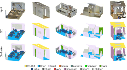
Figure 5: S3DIS results.

4.2 Object Part Segmentation

The performance of our network in object part segmentation is measured by using the ShapeNetPart [Wu et al.(2015)Wu, Song, Khosla, Yu, Zhang, Tang, and Xiao] dataset. This dataset is a collection of 16,681 3D point clouds with 16 categories, each with 2 to 6 part labels. We used the standard train/test splits provided by the dataset. Category mean intersection over union (cat. mIoU) and instance mIoU are used as evaluation metrics. For training, 4096 points are randomly picked and used as input. For testing, the total number of points is used. The evaluation (Table 3) shows that our model is only 0.9% behind the current state of the art in cat. mIoU. Some of the wrong classifications are caused by noisy data, where some object components (e.g. rocket, motorbike, table) are wrongly labeled which is penalized by the metric. Figure 6 shows some qualitative results.

Method	ModelNet40	ShapeNetPart
	OA	cat. mIoU	inst. mIoU
PointNet [Qi et al.(2017a)Qi, Su, Mo, and Guibas]	89.2	80.4	83.7
PointNet++ [Qi et al.(2017b)Qi, Yi, Su, and Guibas]	91.9	81.9	85.1
SO-Net [Li et al.(2018a)Li, Chen, and Lee]	90.9	81.0	84.9
KPConv [Thomas et al.(2019)Thomas, Qi, Deschaud, Marcotegui, Goulette, and Guibas]	92.7	85.1	86.4
PCT [Guo et al.(2020)Guo, Cai, Liu, Mu, Martin, and Hu]	93.2	-	86.4
Ge-Latto (ours)	91.1	84.2	84.5
Ge-Latto (ours fine-tuned)	93.2	-	-

Table 3: ModelNet40 and ShapeNet comparison table.

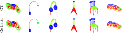
Figure 6: Our ShapeNetPart segmentation results.

4.3 Shape Classification

The ModelNet40 [Yi et al.(2016)Yi, Kim, Ceylan, Shen, Yan, Su, Lu, Huang, Sheffer, and Guibas] dataset is used to study the performance of our network for shape classification. The dataset consists of 12,311 3D meshes and their normal vectors classified into 40 categories. For the experiments, the data is processed similar to Section 4.2. For training, 7,168 points are randomly picked as input, and for testing all the points are used. The evaluation metric is overall accuracy. Our method achieves a competitive result of 91.1% when using the same hyper-parameters and network structure as ShapeNet. If the parameters are fine-tuned, the performance goes up to 93.2%, matching the current best result. More details are given in the ablation study.

4.4 Ablation Study

Auxiliary losses. The auxiliary losses provide a boost in performance to the network. Here, we consider that all weights $\alpha_{i}$ of the auxiliary losses have the same value and vary them from 0 to 1. Table 4 shows that the best performance is obtained with $\alpha_{i}=0.4$, being $1.8\%$ (in terms of mIoU) better than the network trained without auxiliary losses. The supplementary material includes a more comprehensive study for different values of $\alpha_{i}$ on each loss term.

Auxiliary losses			Attention heads			Number of neighbors			Features per multi-head
Aux. weight $\alpha_{i}$	mIoU	mAcc	Attention heads	mIoU	mAcc	k	mIoU	mAcc	N Feat.	mIoU	mAcc
$\alpha_{i}$ = 0.0	67.4	73.2	Only geometric	66.3	72.0	8	64.5	71.8	1	69.2	75.9
$\alpha_{i}$ = 0.2	68.5	74.4	Only features	66.5	72.3	16	66.4	72.1	2	68.2	74.3
$\alpha_{i}$ = 0.4	69.2	75.9	Both	69.2	75.9	32	69.2	75.9	4	68.0	74.2
$\alpha_{i}$ = 0.6	68.6	74.6	MLP+pooling	63.5	69.2	64	-	-	8	68.0	74.1
$\alpha_{i}$ = 0.8	68.3	74.3
$\alpha_{i}$= 1.0	68.1	74.0

Table 4: S3DIS ablation study experiments.

Two-headed attention. Our proposed attention layer is evaluated using different variants: only with the geometric head, only with the feature head, both heads, and no heads (baseline). For the last one, an MLP+pooling layer replaces the attention mechanism. The experiments reported in Table 4 show that only one head is enough to improve the baseline, and that the combination of both heads helps the network in the segmentation task.

Number of neighbors. Three networks with different neighborhood size were trained to find the number of neighbors that provide enough local information. The results from Table 4 show that when $k\leq 16$, the number of neighbors might not be enough to provide a correct representation of the local context; $k=64$ could not fit in the GPU memory.

Features per multi-head. As shown in the supplementary material, each head (geometric and latent) of our attention layer is a special case of a multi-head attention with number of heads $n=D$ or feature dimension $D^{\prime}=1$ per head. For this experiment, the number of features $D^{\prime}$ per head was varied. More features per head means less heads (number of heads $n=D/D^{\prime}$). In other words, $D^{\prime}$ features will be weighted by the same attention score. The results from Table 4 demonstrate that the more features a head has (less number of heads), the less flexible the network becomes. However, reducing the number of heads allows the network to be lighter, because it has to compute only $D/D^{\prime}$ attention scores.

Point cloud classification. The model presented in Section 4 had the same network parameters for all the datasets to show that the proposed method can obtain competitive results without optimizing the hyper-parameters on each dataset. If the hyper-parameters are adjusted for a specific dataset, the performance of the network improves. In this section, the number of sub-sampling points per layer were modified following [Xiang et al.(2021)Xiang, Zhang, Song, Yu, and Cai], where they mainly focus on point cloud classification. By sampling the points using the following values per layer, $N\rightarrow 1024\rightarrow 512\rightarrow 256\rightarrow 64$, instead of $N\rightarrow 4096\rightarrow 2048\rightarrow 512\rightarrow 128$, the overall accuracy of our network increases from 91.1% to 93.2%, matching the state-of-the-art result. This seems to be caused by the number of sampled points and the global average pooling at the end of the encoder layer. Considering that the ModelNet40 dataset has objects with similar parts, like plants with flower pots, if one region of the object is bigger than others, this region will have more sampled points. Because the features of the sampled points at the last layer of the encoder are averaged, if there are more points representing a specific area, the averaged features will have a tendency to represent the wrong part of the object.

Work flow video. The video of our proposed method can be found at: https://youtu.be/mjsttn3C89g. It shows how the point cloud is sampled during the encoder-decoder phase, the auxiliary outputs, and the learned geometric and latent attention weights.

5 Conclusion

This paper proposes a novel two-headed attention mechanism capable of combining the geometric and latent information of neighbor points to learn richer features. This, combined with the leverage provided by the auxiliary losses, allow our network to work with real data and obtain the state of the art in the complex dataset S3DIS for 3D point cloud semantic segmentation. It also gets competitive results in the ShapeNetPart and ModelNet40 datasets.

References

- [Armeni et al.(2016)Armeni, Sener, Zamir, Jiang, Brilakis, Fischer, and Savarese] Iro Armeni, Ozan Sener, Amir R Zamir, Helen Jiang, Ioannis Brilakis, Martin Fischer, and Silvio Savarese. 3d semantic parsing of large-scale indoor spaces. In Proceedings of the IEEE Conference on Computer Vision and Pattern Recognition, pages 1534–1543, 2016.
- [Battaglia et al.(2018)Battaglia, Hamrick, Bapst, Sanchez-Gonzalez, Zambaldi, Malinowski, Tacchetti, Raposo, Santoro, Faulkner, et al.] Peter W Battaglia, Jessica B Hamrick, Victor Bapst, Alvaro Sanchez-Gonzalez, Vinicius Zambaldi, Mateusz Malinowski, Andrea Tacchetti, David Raposo, Adam Santoro, Ryan Faulkner, et al. Relational inductive biases, deep learning, and graph networks. arXiv preprint arXiv:1806.01261, 2018.
- [Choy et al.(2019)Choy, Gwak, and Savarese] Christopher Choy, JunYoung Gwak, and Silvio Savarese. 4d spatio-temporal convnets: Minkowski convolutional neural networks. In Proceedings of the IEEE/CVF Conference on Computer Vision and Pattern Recognition, pages 3075–3084, 2019.
- [Cuevas-Velasquez et al.(2018)Cuevas-Velasquez, Li, Tylecek, Saval-Calvo, and Fisher] Hanz Cuevas-Velasquez, Nanbo Li, Radim Tylecek, Marcelo Saval-Calvo, and Robert B Fisher. Hybrid multi-camera visual servoing to moving target. In 2018 IEEE/RSJ International Conference on Intelligent Robots and Systems (IROS), pages 1132–1137. IEEE, 2018.
- [Cuevas-Velasquez et al.(2020)Cuevas-Velasquez, Gallego, Tylecek, Hemming, Van Tuijl, Mencarelli, and Fisher] Hanz Cuevas-Velasquez, Antonio-Javier Gallego, Radim Tylecek, Jochen Hemming, Bart Van Tuijl, Angelo Mencarelli, and Robert B Fisher. Real-time stereo visual servoing for rose pruning with robotic arm. In 2020 IEEE International Conference on Robotics and Automation (ICRA), pages 7050–7056. IEEE, 2020.
- [Guo et al.(2020)Guo, Cai, Liu, Mu, Martin, and Hu] Meng-Hao Guo, Jun-Xiong Cai, Zheng-Ning Liu, Tai-Jiang Mu, Ralph R Martin, and Shi-Min Hu. Pct: Point cloud transformer. arXiv preprint arXiv:2012.09688, 2020.
- [He et al.(2016)He, Zhang, Ren, and Sun] Kaiming He, Xiangyu Zhang, Shaoqing Ren, and Jian Sun. Deep residual learning for image recognition. In Proceedings of the IEEE conference on computer vision and pattern recognition, pages 770–778, 2016.
- [Hu et al.(2020)Hu, Yang, Xie, Rosa, Guo, Wang, Trigoni, and Markham] Qingyong Hu, Bo Yang, Linhai Xie, Stefano Rosa, Yulan Guo, Zhihua Wang, Niki Trigoni, and Andrew Markham. Randla-net: Efficient semantic segmentation of large-scale point clouds. In Proceedings of the IEEE/CVF Conference on Computer Vision and Pattern Recognition, pages 11108–11117, 2020.
- [Huang et al.(2019)Huang, Zhang, Yi, Funkhouser, Nießner, and Guibas] Jingwei Huang, Haotian Zhang, Li Yi, Thomas Funkhouser, Matthias Nießner, and Leonidas J Guibas. Texturenet: Consistent local parametrizations for learning from high-resolution signals on meshes. In Proceedings of the IEEE/CVF Conference on Computer Vision and Pattern Recognition, pages 4440–4449, 2019.
- [Klokov and Lempitsky(2017)] Roman Klokov and Victor Lempitsky. Escape from cells: Deep kd-networks for the recognition of 3d point cloud models. In Proceedings of the IEEE International Conference on Computer Vision, pages 863–872, 2017.
- [Landrieu and Simonovsky(2018)] Loic Landrieu and Martin Simonovsky. Large-scale point cloud semantic segmentation with superpoint graphs. In Proceedings of the IEEE conference on computer vision and pattern recognition, pages 4558–4567, 2018.
- [Li et al.(2018a)Li, Chen, and Lee] Jiaxin Li, Ben M Chen, and Gim Hee Lee. So-net: Self-organizing network for point cloud analysis. In Proceedings of the IEEE conference on computer vision and pattern recognition, pages 9397–9406, 2018a.
- [Li et al.(2018b)Li, Bu, Sun, Wu, Di, and Chen] Yangyan Li, Rui Bu, Mingchao Sun, Wei Wu, Xinhan Di, and Baoquan Chen. Pointcnn: Convolution on x-transformed points. Advances in neural information processing systems, 31:820–830, 2018b.
- [Lin et al.(2017)Lin, Goyal, Girshick, He, and Dollár] Tsung-Yi Lin, Priya Goyal, Ross Girshick, Kaiming He, and Piotr Dollár. Focal loss for dense object detection. In Proceedings of the IEEE international conference on computer vision, pages 2980–2988, 2017.
- [Lin et al.(2020)Lin, Yan, Huang, Du, Liu, Cui, and Han] Yiqun Lin, Zizheng Yan, Haibin Huang, Dong Du, Ligang Liu, Shuguang Cui, and Xiaoguang Han. Fpconv: Learning local flattening for point convolution. In Proceedings of the IEEE/CVF Conference on Computer Vision and Pattern Recognition, pages 4293–4302, 2020.
- [Liu et al.(2020)Liu, Hu, Cao, Zhang, and Tong] Ze Liu, Han Hu, Yue Cao, Zheng Zhang, and Xin Tong. A closer look at local aggregation operators in point cloud analysis. In European Conference on Computer Vision, pages 326–342. Springer, 2020.
- [Meng et al.(2019)Meng, Gao, Lai, and Manocha] Hsien-Yu Meng, Lin Gao, Yu-Kun Lai, and Dinesh Manocha. Vv-net: Voxel vae net with group convolutions for point cloud segmentation. In Proceedings of the IEEE/CVF International Conference on Computer Vision, pages 8500–8508, 2019.
- [Paszke et al.(2019)Paszke, Gross, Massa, Lerer, Bradbury, Chanan, Killeen, Lin, Gimelshein, Antiga, Desmaison, Kopf, Yang, DeVito, Raison, Tejani, Chilamkurthy, Steiner, Fang, Bai, and Chintala] Adam Paszke, Sam Gross, Francisco Massa, Adam Lerer, James Bradbury, Gregory Chanan, Trevor Killeen, Zeming Lin, Natalia Gimelshein, Luca Antiga, Alban Desmaison, Andreas Kopf, Edward Yang, Zachary DeVito, Martin Raison, Alykhan Tejani, Sasank Chilamkurthy, Benoit Steiner, Lu Fang, Junjie Bai, and Soumith Chintala. Pytorch: An imperative style, high-performance deep learning library. In H. Wallach, H. Larochelle, A. Beygelzimer, F. d'Alché-Buc, E. Fox, and R. Garnett, editors, Advances in Neural Information Processing Systems 32, pages 8024–8035. Curran Associates, Inc., 2019.
- [Qi et al.(2017a)Qi, Su, Mo, and Guibas] Charles R Qi, Hao Su, Kaichun Mo, and Leonidas J Guibas. Pointnet: Deep learning on point sets for 3d classification and segmentation. In Proceedings of the IEEE conference on computer vision and pattern recognition, pages 652–660, 2017a.
- [Qi et al.(2017b)Qi, Yi, Su, and Guibas] Charles R Qi, Li Yi, Hao Su, and Leonidas J Guibas. Pointnet++: Deep hierarchical feature learning on point sets in a metric space. arXiv preprint arXiv:1706.02413, 2017b.
- [Qiu et al.(2021)Qiu, Anwar, and Barnes] Shi Qiu, Saeed Anwar, and Nick Barnes. Semantic segmentation for real point cloud scenes via bilateral augmentation and adaptive fusion. arXiv preprint arXiv:2103.07074, 2021.
- [Riegler et al.(2017)Riegler, Osman Ulusoy, and Geiger] Gernot Riegler, Ali Osman Ulusoy, and Andreas Geiger. Octnet: Learning deep 3d representations at high resolutions. In Proceedings of the IEEE conference on computer vision and pattern recognition, pages 3577–3586, 2017.
- [Shao et al.(2018)Shao, Yang, Weng, Hou, and Zhou] Tianjia Shao, Yin Yang, Yanlin Weng, Qiming Hou, and Kun Zhou. H-cnn: spatial hashing based cnn for 3d shape analysis. IEEE transactions on visualization and computer graphics, 26(7):2403–2416, 2018.
- [Shaw et al.(2018)Shaw, Uszkoreit, and Vaswani] Peter Shaw, Jakob Uszkoreit, and Ashish Vaswani. Self-attention with relative position representations. arXiv preprint arXiv:1803.02155, 2018.
- [Strisciuglio et al.(2018)Strisciuglio, Tylecek, Blaich, Petkov, Biber, Hemming, van Henten, Sattler, Pollefeys, Gevers, et al.] Nicola Strisciuglio, Radim Tylecek, Michael Blaich, Nicolai Petkov, Peter Biber, Jochen Hemming, Eldert van Henten, Torsten Sattler, Marc Pollefeys, Theo Gevers, et al. Trimbot2020: an outdoor robot for automatic gardening. In ISR 2018; 50th International Symposium on Robotics, pages 1–6. VDE, 2018.
- [Tang et al.(2020)Tang, Liu, Zhao, Lin, Lin, Wang, and Han] Haotian Tang, Zhijian Liu, Shengyu Zhao, Yujun Lin, Ji Lin, Hanrui Wang, and Song Han. Searching efficient 3d architectures with sparse point-voxel convolution. In European Conference on Computer Vision, pages 685–702. Springer, 2020.
- [Tatarchenko et al.(2018)Tatarchenko, Park, Koltun, and Zhou] Maxim Tatarchenko, Jaesik Park, Vladlen Koltun, and Qian-Yi Zhou. Tangent convolutions for dense prediction in 3d. In Proceedings of the IEEE Conference on Computer Vision and Pattern Recognition, pages 3887–3896, 2018.
- [Tchapmi et al.(2017)Tchapmi, Choy, Armeni, Gwak, and Savarese] Lyne Tchapmi, Christopher Choy, Iro Armeni, JunYoung Gwak, and Silvio Savarese. Segcloud: Semantic segmentation of 3d point clouds. In 2017 international conference on 3D vision (3DV), pages 537–547. IEEE, 2017.
- [Thomas et al.(2019)Thomas, Qi, Deschaud, Marcotegui, Goulette, and Guibas] Hugues Thomas, Charles R Qi, Jean-Emmanuel Deschaud, Beatriz Marcotegui, François Goulette, and Leonidas J Guibas. Kpconv: Flexible and deformable convolution for point clouds. In Proceedings of the IEEE/CVF International Conference on Computer Vision, pages 6411–6420, 2019.
- [Vaswani et al.(2017)Vaswani, Shazeer, Parmar, Uszkoreit, Jones, Gomez, Kaiser, and Polosukhin] Ashish Vaswani, Noam Shazeer, Niki Parmar, Jakob Uszkoreit, Llion Jones, Aidan N Gomez, Lukasz Kaiser, and Illia Polosukhin. Attention is all you need. arXiv preprint arXiv:1706.03762, 2017.
- [Wang et al.(2017)Wang, Liu, Guo, Sun, and Tong] Peng-Shuai Wang, Yang Liu, Yu-Xiao Guo, Chun-Yu Sun, and Xin Tong. O-cnn: Octree-based convolutional neural networks for 3d shape analysis. ACM Transactions on Graphics (TOG), 36(4):1–11, 2017.
- [Wu et al.(2019)Wu, Qi, and Fuxin] Wenxuan Wu, Zhongang Qi, and Li Fuxin. Pointconv: Deep convolutional networks on 3d point clouds. In Proceedings of the IEEE/CVF Conference on Computer Vision and Pattern Recognition, pages 9621–9630, 2019.
- [Wu et al.(2015)Wu, Song, Khosla, Yu, Zhang, Tang, and Xiao] Zhirong Wu, Shuran Song, Aditya Khosla, Fisher Yu, Linguang Zhang, Xiaoou Tang, and Jianxiong Xiao. 3d shapenets: A deep representation for volumetric shapes. In Proceedings of the IEEE conference on computer vision and pattern recognition, pages 1912–1920, 2015.
- [Xiang et al.(2021)Xiang, Zhang, Song, Yu, and Cai] Tiange Xiang, Chaoyi Zhang, Yang Song, Jianhui Yu, and Weidong Cai. Walk in the cloud: Learning curves for point clouds shape analysis. arXiv preprint arXiv:2105.01288, 2021.
- [Yang et al.(2020)Yang, Liu, Pan, Liu, and Tong] Yuqi Yang, Shilin Liu, Hao Pan, Yang Liu, and Xin Tong. Pfcnn: convolutional neural networks on 3d surfaces using parallel frames. In Proceedings of the IEEE/CVF Conference on Computer Vision and Pattern Recognition, pages 13578–13587, 2020.
- [Yi et al.(2016)Yi, Kim, Ceylan, Shen, Yan, Su, Lu, Huang, Sheffer, and Guibas] Li Yi, Vladimir G Kim, Duygu Ceylan, I-Chao Shen, Mengyan Yan, Hao Su, Cewu Lu, Qixing Huang, Alla Sheffer, and Leonidas Guibas. A scalable active framework for region annotation in 3d shape collections. ACM Transactions on Graphics (ToG), 35(6):1–12, 2016.
- [Zhao et al.(2017)Zhao, Shi, Qi, Wang, and Jia] Hengshuang Zhao, Jianping Shi, Xiaojuan Qi, Xiaogang Wang, and Jiaya Jia. Pyramid scene parsing network. In Proceedings of the IEEE conference on computer vision and pattern recognition, pages 2881–2890, 2017.
- [Zhao et al.(2020)Zhao, Jia, and Koltun] Hengshuang Zhao, Jiaya Jia, and Vladlen Koltun. Exploring self-attention for image recognition. In Proceedings of the IEEE/CVF Conference on Computer Vision and Pattern Recognition, pages 10076–10085, 2020.
- [Zhou and Tuzel(2018)] Yin Zhou and Oncel Tuzel. Voxelnet: End-to-end learning for point cloud based 3d object detection. In Proceedings of the IEEE Conference on Computer Vision and Pattern Recognition, pages 4490–4499, 2018.