Random matrices associated with general barrier billiards

Abstract

The paper is devoted to the derivation of random unitary matrices whose spectral statistics is the same as statistics of quantum eigenvalues of certain deterministic two-dimensional barrier billiards. These random matrices are extracted from the exact billiard quantisation condition by applying a random phase approximation for high-excited states. An important ingredient of the method is the calculation of $S$-matrix for the scattering in the slab with a half-plane inside by the Wiener-Hopf method. It appears that these random matrices have the form similar to the one obtained by the author in [arXiv:2107.03364] for a particular case of symmetric barrier billiards but with different choices of parameters. The local correlation functions of the resulting random matrices are well approximated by the semi-Poisson distribution which is a characteristic feature of various models with intermediate statistics. Consequently, local spectral statistics of the considered barrier billiards is (i) universal for almost all values of parameters and (ii) well described by the semi-Poisson statistics.

I Introduction

Polygonal billiards constitute a special class of classical dynamical systems. Though they have zero Lyapunov exponents the behaviour of their trajectories is intricate and complicated due to, in general, unavoidable discontinuities of the ray dynamics (see, e.g., gutkin ). An important subset of polygonal billiards is constituted by the so-called pseudo-integrable billiards (see, e.g., richens_berry ) characterised by the requirement that all their angles $\theta_{j}$ are rational multiples of $\pi$

$$\theta_{j}=\frac{m_{j}}{n_{j}}\pi$$ (1)

with co-prime integers $m_{j}$ and $n_{j}$. A characteristic property of pseudo-integrable billiards is the fact that their trajectories cover surfaces of finite genus connected with angles by the formula katok

$$g=1+\frac{N_{n}}{2}\sum_{j}\frac{m_{j}-1}{n_{j}}$$ (2)

where $N_{n}$ is the least common multiply of all denominators $n_{j}$. This is a clear-cut difference of pseudo-integrable billiards (with at least one $m_{j}>1$) from both limiting cases of classical dynamical models: integrable models where trajectories belong to tori (i.e., surfaces with $g=1$) and chaotic models where a typical trajectory covers the whole surface of constant energy.

It is plain that peculiarities of pseudo-integrable billiards should have quantum manifestations but no general statements about statistical properties of pseudo-integrable models have been proposed so far. It is in a strong contrast with quantum integrable and fully chaotic models where the well-known and well-accepted conjectures were established long time ago berry_tabor and BGS . Numerical results cheon -gorin_wiersig suggest that, at least, for certain pseudo-integrable billiards spectral statistics differs from both the Poisson statistics of integrable models berry_tabor as well as from the usual random matrix statistics conjectured for chaotic motels BGS . Surprisingly, the observed statistics (called intermediate statistics) is similar to the spectral statistics of the Anderson model at the point of metal-insulator transition altshuler ; shklovskii whose main features are (i) linear level repulsion as for usual random matrix ensembles and (ii) an exponential fall-off of nearest-neighbour distributions as for the Poisson distribution.

The simplest pseudo-integrable model is a rectangular billiard with a barrier inside (see figure 1(a)). It has 6 internal angles equal $\pi/2$ and one angle $2\pi$. According to (2) it corresponds to a genus 2 surface. Quantum problem for such billiards consists in finding eigenvalues $k$ and eigenfunctions $\Psi(x,y;k)$ of the Helmholtz equation

$$\left(\Delta+k^{2}\right)\Psi(x,y;k)=0$$ (3)

provided that functions $\Psi(x,y;k)$ obey the Dirichlet boundary conditions

$$\Psi(x,y;k)|_{\mathrm{boundaries}}=0.$$ (4)

Generalisation for another type of boundary conditions is straightforward.

Numerical calculations wiersig ; gorin_wiersig were done exclusively for a symmetric barrier billiard with $h=b/2$. A new method of extracting random matrices from the exact quantisation of a symmetric barrier billiard has been proposed in bogomolny . The main conclusion of that paper is that spectral statistics of symmetric barrier billiard is the same as the one for a $N\times N$ random unitary matrix

$$B_{\mu,\nu}=e^{i\Phi_{\mu}}\frac{L_{\mu}L_{\nu}}{x_{\mu}+x_{\nu}},\qquad\mu,\nu=1,\ldots N$$ (5)

where $\Phi_{\mu}$ are independent real random variables distributed uniformly between $0$ and $2\pi$. $L_{\mu}$ are real quantities determined by the expression

$$L_{\mu}^{2}=2x_{\mu}\prod_{\nu\neq\mu}\frac{x_{\mu}+x_{\nu}}{x_{\mu}-x_{\nu}}$$ (6)

and coordinates $x_{\mu}$ for a symmetric barrier billiard (with $h=b/2$) are

$$x_{\mu}=(-1)^{\mu+1}\sqrt{k^{2}-\frac{\pi^{2}\mu^{2}}{b^{2}}}\,.$$ (7)

The condition that all $x_{\mu}$ are real defines matrix dimension $N$

$$N=\left[\frac{kb}{\pi}\right]$$ (8)

where $[x]$ is the largest integer less or equal $x$.

(a)

(b)

Figure 1: Barrier billiards considered in the paper. For clarity the barrier tip is indicated by a small circle.

The purpose of the paper is to generalise the method of bogomolny for non-symmetric barrier billiards shown in figure 1. It appears that the random matrix extracted from the exact quantisation condition for these billiards also have the form given by (5) and (6) but with a different specification of coordinates $x_{\mu}$.

The plan of the paper is the following. Section II is devoted to the discussion of the surface-of-section method in application to barrier billiards proposed in bogomolny . The method consists in opening the billiard and finding exact scattering solutions for the resulting slab with a half-plane inside. Writing exact eigenfunctions of a barrier billiard as a linear combination of scattering waves and imposing the correct boundary conditions on previously removed parts of billiard boundary gives the quantisation condition in the form $\det(1+B)=0$ where matrix $B$ differs form the $S$-matrix for the scattering in the slab by certain phase-like factors. It is known that spectral statistics of matrix $B$ is up to a rescaling coincides with statistics of high-excited barrier billiard eigenenergies semiclassics ; DS . The main part of the paper consists in the calculation of the exact scattering $S$-matrix by the Wiener-Hopf method. This is done in Section III. As it is typical for the Wiener-Hopf method the resulting expressions include infinite products and are quite cumbersome. In Section IV two important simplifications appeared in the semiclassical limit are discussed. First, by ignoring exponentially decreasing evanescent modes one gets finite dimensional unitary $S$ and $B$ matrices. Second, the phase factors by which the $B$-matrix differs from the $S$-matrix are considered as independent random variables uniformly distributed on the unit circles. Noticing that proper $S$-matrix phases by conjugation lead only to a shift of random phases of the $B$-matrix one proves that the resulting unitary random matrix has the form (5) and (6) but a different definition of coordinates $x_{\mu}$. In has been argued in bogomolny that local correlation functions of such matrices should be well described by the semi-Poisson distribution appeared in different models with intermediate statistics plasma_model . This statement is illustrated by numerical calculations for certain typical barrier billiard parameters in the end of Section IV. Section V is a brief recapitulation of the main steps permitting to extract random matrices from the exact solution of barrier billiard problems. Appendix A presents the factorisation of the kernel appeared in the Wiener-Hopf method and the explicit verification of the unitarity of the obtained scattering $S$-matrix.

II Exact surface-of-section quantisation

The first step of the method proposed in bogomolny consists in the removal boundaries perpendicular to the barrier and considering instead of a closed system the problem of a scattering inside an infinite slab of height $b$ with a half-plane inside as indicated in figure 2. The Dirichlet boundary conditions (4) are imposed in all boundaries.

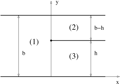
Figure 2: An infinite slab with a half-plane inside. Numbers indicate 3 possible channels.

Inside the slab there exit 3 different regions (channels) (see figure 2). The following functions constitute elementary solutions in these channels (normalised to unit current)

$$\phi_{n}^{(\beta)\pm}(x,y)=\frac{e^{\pm ip_{n}^{(\beta)}x}}{\sqrt{h_{\beta}p_{n}^{(\beta)}}}\sin\Big{(}\frac{\pi n}{h_{\beta}}y\Big{)},\qquad p_{n}^{(\beta)}=\sqrt{k^{2}-\frac{\pi^{2}n^{2}}{h_{\beta}^{2}}},\qquad\beta=1,2,3\,.$$ (9)

Here $h_{\beta}$ is the width of channel $\beta$

$$h_{1}=b,\quad h_{2}=b-h,\quad h_{3}=h.$$ (10)

By definition, these functions are zero outside the corresponding channels. Subscript $(+)$ (resp., $(-)$) indicates plane waves propagating from left to right (resp., from right to left).

We consider 3 different solutions corresponded to 3 possible plane waves entering from the infinity into the indicated regions of the slab. They are denoted by $\Psi_{n}^{(\beta)}(x,y)$ where superscript $(\beta)$ with $\beta=1,2,3$ indicates the entering channel and subscript $n$ is the transverse quantum number of the incident plane wave. Their formal expansions into elementary solutions (9) are

$$\Psi_{n}^{(1)}(x,y) = \phi_{n}^{(1)+}(x,y)+\sum_{m=1}^{\infty}\left[S_{n,m}^{1\to 1}\phi_{m}^{(1)-}(x,y)+S_{n,m}^{1\to 2}\phi_{m}^{(2)+}(x,y)+S_{n,m}^{1\to 3}\phi_{m}^{(3)+}(x,y)\right],$$ (11)

$$\Psi_{n}^{(2)}(x,y) = \phi_{n}^{(2)-}(x,y)+\sum_{m=1}^{\infty}\left[S_{n,m}^{2\to 1}\phi_{m}^{(1)-}(x,y)+S_{n,m}^{2\to 2}\phi_{m}^{(2)+}(x,y)+S_{n,m}^{2\to 3}\phi_{m}^{(3)+}(x,y)\right],$$ (12)

$$\Psi_{n}^{(3)}(x,y) = \phi_{n}^{(3)-}(x,y)+\sum_{m=1}^{\infty}\left[S_{n,m}^{3\to 1}\phi_{m}^{(1)-}(x,y)+S_{n,m}^{3\to 2}\phi_{m}^{(2)+}(x,y)+S_{n,m}^{3\to 3}\phi_{m}^{(3)+}(x,y)\right].$$ (13)

The first terms are the incident plane waves with momentum $p_{n}^{(\beta)}$ and the remaining sums represent the reflected and transmitted waves in all channels.

Coefficients $S_{n,m}^{\alpha\to\beta}$ with $\alpha,\beta=1,2,3$ form the $S$-matrix for the scattering inside the slab indicated in figure (2). In the next Section it will be calculated analytically by the Wiener-Hopf method.

When these coefficients are known, functions (11)-(13) are solutions of the Helmholtz equation (3) obeying the correct boundary conditions on all horizontal boundaries. Let us construct an eigenfunction of barrier billiards indicated in figure 1 as a linear combination of all scattering waves

$$\Psi(x,y;k)=\sum_{n=1}^{\infty}\sum_{\alpha=1}^{3}a_{n}^{(\alpha)}\Psi_{n}^{(\alpha)}(x,y)\,.$$ (14)

Coefficients $a_{n}^{(\alpha)}$ have to be determined from the requirement that this wave obeys the correct boundary conditions on vertical boundaries. For the general billiard as in figure 1(b) these conditions are

$$\Psi(d_{1},y;k) = 0,\qquad h<y<b,$$ (15)

$$\Psi(d_{2},y;k) = 0,\qquad 0<y<h,$$ (16)

$$\Psi(d_{2}-a,y;k) = 0,\qquad 0<y<b.$$ (17)

In each channel function $\Psi_{n}(x,y)$ is a linear combination of elementary solutions (9) which form a complete and orthogonal set of functions of $y$. Therefore, the Dirichlet boundary conditions (15)-(17) imply that the coefficients of these linear combinations have to be zero. It means that $a_{n}^{(\alpha)}$ are determined from the equations

$$a_{m}^{(\beta)}+e^{i\phi_{m}^{(\beta)}}\sum_{n=1}^{\infty}\sum_{\alpha=1}^{3}a_{n}^{(\alpha)}S_{n,m}^{\alpha\to\beta}=0,\qquad\beta=1,2,3\,.$$ (18)

Here quantities $\phi_{m}^{(\alpha)}$ are

$$\phi_{m}^{(1)}=2p_{m}^{(1)}(a-d_{2}),\qquad\phi_{m}^{(2)}=2p_{m}^{(2)}d_{1},\qquad\phi_{m}^{(3)}=2p_{m}^{(3)}d_{2}\,.$$ (19)

These relations can compactly be rewritten as follows (with the standard convention that the summation is performed over repeated indices)

$$a_{m}^{(\beta)}+a_{n}^{(\alpha)}B_{n,m}^{\alpha\to\beta}=0$$ (20)

where

$$B_{n,m}^{\alpha\to\beta}=e^{i\phi_{m}^{(\beta)}}S_{n,m}^{\alpha\to\beta}\,.$$ (21)

Matrix $B$ has two groups of indices, $\alpha,\beta=1,2,3$ indicate the initial and final channels and indices $n,m$ are positive integers denoted transverse quantum numbers of waves propagating in these channels.

The condition of compatibility of these equation (i.e., the quantisation condition on momentum $k$) is

$$\det(\delta_{m,n}\delta_{\alpha,\beta}+B_{n,m}^{\alpha\to\beta})=0\,.$$ (22)

III Calculation of scattering $S$-matrix

To use the formulas of the preceding Section it is necessary to know the $S$-matrix which describes the scattering inside the slab with a half-plane inside (cf., figure 2). A convenient (and probably the simplest) way to calculate it is to use the Wiener-Hopf method. It is an old, powerful, and well known method of solving certain diffraction-like problems (see, e.g., noble and references therein) by reduction them to a special equation (called the scalar Wigher-Hopf equation) of the following form

$$K(\alpha)X_{+}(\alpha)+X_{-}(\alpha)=f(\alpha)\,.$$ (23)

Here $X_{+}(\alpha)$ and $X_{-}(\alpha)$ are two unknown functions of complex variable $\alpha$. Functions $K(\alpha)$ and $f(\alpha)$ are supposed to be known.

The essence of the Wiener-Hopf method is the assumption that function $X_{+}(\alpha)$ is free from singularities in the upper half-plane $\mathrm{Im}\,\alpha>-\epsilon_{1}$ and function $X_{-}(\alpha)$ has no singularities in the lower half-plane $\mathrm{Im}\,\alpha<\epsilon_{2}$ with $\epsilon_{1,2}>0$. These requirements are usually achieved by representing functions $X_{\pm}(\alpha)$ as one-sided Fourier transforms

$$X_{+}(\alpha)=\int_{0}^{\infty}\psi(x)e^{i\alpha x}dx,\qquad X_{-}(\alpha)=\int_{-\infty}^{0}\psi(x)e^{i\alpha x}dx$$ (24)

where function $\psi(x)$ exponentially decays at $|x|\to\infty$

$$\psi(x)\underset{x\to+\infty}{\longrightarrow}e^{-\epsilon_{1}x},\qquad\psi(x)\underset{x\to-\infty}{\longrightarrow}e^{\epsilon_{2}x}.$$ (25)

The solution the Wiener-Hopf equation (23) consists in the following steps (see noble for details and proofs).

• Factorise the kernel $K(\alpha)$ into a product of two functions $K(\alpha)=K_{+}(\alpha)K_{-}(\alpha)$ where functions $K_{\pm}(\alpha)$ are free of singularities and zeros in, respectively, upper and lower half-planes.

• Divide the both parts of (23) by $K_{-}(\alpha)$

  $$K_{+}(\alpha)X_{+}(\alpha)+\frac{X_{-}(\alpha)}{K_{-}(\alpha)}=\frac{f(\alpha)}{K_{-}(\alpha)}.$$ (26)

• Represent the right-hand side of this equation as a sum of functions $F_{\pm}(\alpha)$ free of singularities in the corresponding half-planes

  $$\frac{f(\alpha)}{K_{-}(\alpha)}=F_{+}(\alpha)+F_{-}(\alpha).$$ (27)

• After such transformation the Wiener-Hopf equation becomes

  $$\frac{X_{-}(\alpha)}{K_{-}(\alpha)}-F_{-}(\alpha)=F_{+}(\alpha)-K_{+}(\alpha)X_{+}(\alpha).$$ (28)

By construction the left-hand side of this equation is free of singularities in the lower half-plane $\mathrm{Im}\,\alpha<\epsilon_{2}$ and the right-hand side has no singularities in the upper half-plane $\mathrm{Im}\,\alpha>-\epsilon_{1}$. As these planes have a common part, the both parts have to be free of singularities in the whole complex plane of $\alpha$. Therefore they have to be a polynomial in $\alpha$. Usually from the boundary conditions it follows that this polynomial is zero. It such case the solutions of the Wiener-Hopf equation are

$$X_{-}(\alpha)=K_{-}(\alpha)F_{-}(\alpha),\qquad X_{+}(\alpha)=\frac{F_{+}(\alpha)}{K_{+}(\alpha)}\,.$$ (29)

The reduction of a given problem to the Wiener-Hopf equation (when it is possible) can be done by different methods. Below we follow the one discussed in noble .

A solution of a scattering problem for the Helmholtz equation consists of two parts, an incident wave and a reflected wave

$$\Psi(x,y)=\Psi_{\mathrm{inc}}(x,y)+\psi_{\mathrm{ref}}(x,y).$$ (30)

Assume that momentum $k$ in (3) has a small positive imaginary part: $k\to k+i\delta k$. Then it is known that the reflected wave tends to zero when $|x|\to\infty$ (this is the radiation condition). From expansions similar to (11)-(13) it follows that $\psi_{\mathrm{ref}}(x,y)\longrightarrow e^{-r\delta k|x|}$ with $r\geq 1$. Therefore one can take $\epsilon_{1}=\epsilon_{2}=\delta k$ and the following quantities

$$\Phi_{+}(\alpha,y)=\int_{0}^{\infty}\psi_{\mathrm{ref}}(x,y)e^{i\alpha x}dx,\qquad\Phi_{-}(\alpha,y)=\int_{-\infty}^{0}\psi_{\mathrm{ref}}(x,y)e^{i\alpha x}dx$$ (31)

are free of singularities in, respectively, the upper half-plane $\mathrm{Im}\,\alpha>-\delta k$ and the lower half-plane $\mathrm{Im}\,\alpha<\delta k$.

As $\Psi_{\mathrm{inc}}(x,y)$ and $\psi_{\mathrm{ref}}(x,y)$ obey the Helmholtz equation (3) quantities $\Phi_{\pm}(\alpha,y)$ have to obey the equation

$$\Big{(}\frac{\partial^{2}}{\partial y^{2}}+q^{2}(\alpha)\Big{)}\Phi_{\pm}(\alpha,y)=0,\qquad q^{2}(\alpha)=k^{2}-\alpha^{2}\,.$$ (32)

Because there are no obstacles in the horizontal directions, the necessary solutions which are zero at horizontal boundaries of the slab are

$$\Phi_{+}(\alpha,y)+\Phi_{-}(\alpha,y)=\left\{\begin{array}[]{lc}A(\alpha)\sin\big{(}q(\alpha)y\big{)},&0<y<h\\ B(\alpha)\sin\big{(}q(\alpha)(b-y)\big{)},&h<y<b\end{array}\right..$$ (33)

When functions $A(\alpha)$ and $B(\alpha)$ are calculated, the reflection field is given by the inverse Fourier transformation

$$\psi(x,y)=\frac{1}{2\pi}\int_{-\infty}^{\infty}e^{-i\alpha x}d\alpha\left\{\begin{array}[]{l c}A(\alpha)\sin\big{(}q(\alpha)y\big{)},&0<y<h\\ B(\alpha)\sin\big{(}q(\alpha)(b-y)\big{)},&h<y<b\end{array}\right..$$ (34)

For positive $x$ the integration contour can be shifted in the lower half-plane of $\alpha$ and for negative $x$ one can shift the contour into the upper half-plane.

To find uniquely functions $\Phi_{\pm}(\alpha,y)$ it is necessary to know their values at the line $y=h$ which follow from general properties of wave functions.

• At the half-line $y=h$, $0<x<\infty$ the total field has to be zero, $\Psi(x,h)=0$. It means that

  $$\int_{0}^{\infty}\Psi_{\mathrm{inc}}(x,h)e^{i\alpha x}dx+\Phi_{+}(\alpha,h)=0.$$ (35)

• The total field $\Psi(x,y)$ and its $y$-derivative $\Psi^{\prime}(x,y)$ have to be continuous at $y=h$ and negative $x$. The incident waves for all 3 solutions is continuous at $y=h$ but their $y$-derivatives have a jump for the second and third solutions. It leads to the following relation (^′ indicates the derivative over $y$)

  $$\int_{-\infty}^{0}\left(\Psi_{\mathrm{inc}}^{\prime}(x,h+0)-\Psi_{\mathrm{inc}}^{\prime}(x,h-0)\right)e^{i\alpha x}dx+\left(\Phi_{-}^{\prime}(x,h+0)-\Phi_{-}^{\prime}(x,h-0)\right)=0.$$ (36)

It appears that the 3 scattering solutions (11)-(13) lead to Eq. (23) with the same kernel $K(\alpha)$ but with different right-hand sides. For completeness the calculations are sketched below.

III.1 First solution

For this solution the incident field $\Psi_{\mathrm{inc}}(x,y)=\phi_{n}^{(1)+}(x,y)$ (cf. (11)). From (35) it follows that

$$\Phi_{+}(\alpha,h)=-\frac{i\sin(\pi nh/b)}{\big{(}\alpha+p_{n}^{(1)}\big{)}\sqrt{bp_{n}^{(1)}}}\,.$$ (37)

From (33) one gets

$$\Phi_{-}(\alpha,h)-\frac{i\sin(\pi nh/b)}{\big{(}\alpha+p_{n}^{(1)}\big{)}\sqrt{bp_{n}^{(1)}}}=A(\alpha)\sin\big{(}q(\alpha)h\big{)}=B(\alpha)\sin\big{(}q(\alpha)(b-h)\big{)}\,.$$ (38)

Calculation of the $y$-derivative of the total field at the both sides of the barrier $y=h$, $x>0$ gives the following equations

$$\Phi_{+}^{\prime}(\alpha,h+0)+\Phi_{-}^{\prime}(\alpha,h) = -q(\alpha)B(\alpha)\cos\big{(}q(\alpha)(b-h)\big{)},$$

$$\Phi_{+}^{\prime}(\alpha,h-0)+\Phi_{-}^{\prime}(\alpha,h) = q(\alpha)A(\alpha)\cos\big{(}q(\alpha)h\big{)}.$$ (39)

Denoting $X_{+}(\alpha)=b\big{(}\Phi_{+}^{\prime}(\alpha,h+0)-\Phi_{+}^{\prime}(\alpha,h-0)\big{)}$ one finds

$$X_{+}(\alpha)=-bq(\alpha)\Big{(}A(\alpha)\cos\big{(}q(\alpha)h\big{)}+B(\alpha)\cos\big{(}q(\alpha)(b-h)\big{)}\Big{)}\,.$$ (40)

Using (38) one can express $A(\alpha)$ and $B(\alpha)$ through $\Phi_{-}(\alpha,h)\equiv X_{-}(\alpha)$. It gives the final Wiener-Hopf equation (23) with

$$K(\alpha)=\frac{\sin\big{(}q(\alpha)h\big{)}\sin\big{(}q(\alpha)(b-h)\big{)}}{bq(\alpha)\sin\big{(}q(\alpha)b\big{)}}$$ (41)

and

$$f_{1}(\alpha)=\frac{i\sin(\pi nh/b)}{\big{(}\alpha+p_{n}^{(1)}\big{)}\sqrt{bp_{n}^{(1)}}}.$$ (42)

The necessary factorisation $K(\alpha)=K_{+}(\alpha)K_{-}(\alpha)$ is discussed in Appendix A.

For the decomposition (27) it is necessary to remove the pole $\alpha=-p_{n}^{(1)}$ from $F_{-}(\alpha)$. In such way one obtains

$$F_{-}(\alpha)=f_{1}(\alpha)\left(\frac{1}{K_{-}(\alpha)}-\frac{1}{K_{-}(-p_{n}^{(1)})}\right),\qquad F_{+}(\alpha)=\frac{f_{1}(\alpha)}{K_{-}(-p_{n}^{(1)})}\,.$$ (43)

Using (29) and (38) leads to the following expressions

$$A(\alpha)=\frac{C_{1}(\alpha)}{\sin\big{(}q(\alpha)h\big{)}},\qquad B(\alpha)=\frac{C_{1}(\alpha)}{\sin\big{(}q(\alpha)(b-h)\big{)}}$$ (44)

where

$$C_{1}(\alpha)=-\frac{i\sin(\pi nh/b)K_{-}(\alpha)}{\big{(}\alpha+p_{n}^{(1)}\big{)}K_{-}(-p_{n}^{(1)})\sqrt{bp_{n}^{(1)}}}\,.$$ (45)

III.2 Second solution

For these solution the incident wave $\Psi_{\mathrm{inc}}=\phi_{n}^{(2)-}(x,y)$ (see (12)). Therefore from (35) it follows that

$$\Phi_{+}(\alpha,h)=0$$ (46)

and, consequently,

$$X_{-}(\alpha)\equiv\Phi_{-}(\alpha,h)=A(\alpha)\sin\big{(}q(\alpha)h\big{)}=B(\alpha)\sin\big{(}q(\alpha)(b-h)\big{)}.$$ (47)

The incident field $\phi_{n}^{(2)-}(x,y)$ is continuous at $y=h$, $-\infty<x<0$ but its $y$ derivative has a jump at this line. Therefore, $\Phi_{-}(\alpha,y)$ is also continuous at this line but its $y$-derivative should compensate the discontinuity of $y$ derivative of the incident field (cf. (36)). It means that

$$\Phi_{-}^{\prime}(\alpha,h+0)-\Phi_{-}^{\prime}(\alpha,h-0)=-\frac{i\pi(-1)^{n}n}{(b-h)\big{(}\alpha-p_{n}^{(2)}\big{)}\sqrt{(b-h)p_{n}^{(2)}}}\,.$$ (48)

Comparing the $y$-derivatives from the both sides of $y=h$ with (33) gives the following equation

$$X_{+}(\alpha)\equiv b\left(\Phi_{+}^{\prime}(\alpha,h+0)-\Phi_{+}^{\prime}(\alpha,h-0)\right)=$$

$$= \frac{i\pi(-1)^{n}n\,b}{(b-h)\big{(}\alpha-p_{n}^{(2)}\big{)}\sqrt{(b-h)p_{n}^{(2)}}}-bq(\alpha)\left(B(\alpha)\cos\big{(}q(\alpha)(b-h)\big{)}+A(\alpha)\cos\big{(}q(\alpha)h\big{)}\right)\,.$$

Expressing $A(\alpha)$ and $B(\alpha)$ from (47) leads to the Wiener-Hopf equation (23) with $K(\alpha)$ given by (41) and

$$f_{2}(\alpha)=\frac{i\pi(-1)^{n}nbK(\alpha)}{(b-h)\big{(}\alpha-p_{n}^{(2)}\big{)}\sqrt{(b-h)p_{n}^{(2)}}}\,.$$ (50)

Solving the resulting Wiener-Hopf equation equation and using (47) one gets

$$A(\alpha)=\frac{C_{2}(\alpha)}{\sin\big{(}q(\alpha)h\big{)}},\qquad B(\alpha)=\frac{C_{2}(\alpha)}{\sin\big{(}q(\alpha)(b-h)\big{)}}$$ (51)

where

$$C_{2}(\alpha)=\frac{i\pi(-1)^{n}nb\,K_{+}(p_{n}^{(2)})K_{-}(\alpha)}{(b-h)\big{(}\alpha-p_{n}^{(2)}\big{)}\sqrt{(b-h)p_{n}^{(2)}}}\,.$$ (52)

III.3 Third solution

In this case the incident field $\Psi_{\mathrm{inc}}=\phi_{n}^{(3)-}(x,y)$ and Eqs. (46) and (47) remain valid.

From discontinuity of the incident field one gets

$$\Phi_{-}^{\prime}(\alpha,h+0)-\Phi_{-}^{\prime}(\alpha,h-0)=-\frac{i(-1)^{n}\pi n}{h\big{(}\alpha-p_{n}^{(3)}\big{)}\sqrt{hp_{n}^{(3)}}}.$$ (53)

As above one obtains the same Wiener-Hopf equation but with

$$f_{3}(\alpha)=\frac{i(-1)^{n}\pi nbK(\alpha)}{h\big{(}\alpha-p_{n}^{(3)}\big{)}\sqrt{hp_{n}^{(3)}}}\,.$$ (54)

In this case one finds

$$A(\alpha)=\frac{C_{3}(\alpha)}{\sin\big{(}q(\alpha)h\big{)}},\qquad B(\alpha)=\frac{C_{3}(\alpha)}{\sin\big{(}q(\alpha)(b-h)\big{)}}$$ (55)

with

$$C_{3}(\alpha)=\frac{i(-1)^{n}\pi nb\,K_{+}(p_{n}^{(3)})K_{-}(\alpha)}{h\big{(}\alpha-p_{n}^{(3)}\big{)}}\,.$$ (56)

III.4 $S$-matrix for irrational $h/b$

Finding the reflection field by the inverse Fourier transform (34) and using the relation $K_{-}(-\alpha)=K_{+}(\alpha)$ after simple but tedious calculations one gets the explicit form of the $S$-matrix

$$S_{n,m}^{\alpha\to\beta}=\frac{L_{n}^{(\alpha)}L_{m}^{(\beta)}}{x_{n}^{(\alpha)}+x_{m}^{(\beta)}}$$ (57)

where

$$L_{n}^{(1)}=\frac{\sin\big{(}\pi nh/b\big{)}}{K_{+}(p_{n}^{(1)})\sqrt{bp_{n}^{(1)}}},\quad L_{n}^{(2)}=-\frac{(-1)^{n}\pi nb\,K_{+}(p_{n}^{(2)})}{(b-h)\sqrt{(b-h)p_{n}^{(2)}}},\quad L_{n}^{(3)}=-\frac{(-1)^{n}\pi nb\,K_{+}(p_{n}^{(3)})}{h\sqrt{hp_{n}^{(3)}}}$$ (58)

and

$$x_{n}^{(1)}=bp_{n}^{(1)},\qquad x_{n}^{(2)}=-bp_{n}^{(2)},\qquad x_{n}^{(3)}=-bp_{n}^{(3)}.$$ (59)

Function $K_{+}(\alpha)$ is given by (convergent) infinite product (89) and values of momenta $p_{m}^{(\beta)}$ with $\beta=1,2,3$ are indicated in (9).

Notice that the $S$-matrix is symmetric as it should be from the reciprocity principle.

The above expressions are valid when the ratio $h/b$ is an irrational number which means that (i) $\sin\big{(}\pi hn/b\big{)}\neq 0$ for all $n$ and (ii) all $p_{m}^{(\alpha)}$ are different. For rational $h/b$ certain terms in the above formulas will have formally uncertainties of $0/0$ type. Though they can be resolved by taking a corresponding limit it is more convenient to reconsider the resonance case separately.

III.5 $S$-matrix for rational $h/b$

Let, for simplicity, $h/b=1/q$ with integer $q$. In this case the following 3 moments are equal

$$p_{n}^{(3)}=p_{(q-1)n}^{(2)}=p_{qn}^{(1)}$$ (60)

and it is plain that waves $\psi^{(1)\pm}_{qn}(x,y)$ are two exact solutions of the problem considered as they are automatically zero on the full line passing through the barrier. As

$$\frac{1}{\sqrt{bp_{qn}^{(1)}}}\sin\left(\frac{\pi qn}{b}y\right)=\left\{\begin{array}[]{cc}\frac{1}{\sqrt{hp_{n}^{(3)}}}\sin\Big{(}\frac{\pi n}{h}y\Big{)}\sqrt{\frac{h}{b}},&0<y<h\\ \frac{1}{\sqrt{(b-h)p_{(q-1)n}^{(2)}}}\sin\Big{(}\frac{\pi(q-1)n}{b-h}(b-y)\Big{)}(-1)^{nq+1}\sqrt{\frac{b-h}{b}},&h<y<b\end{array}\right.$$ (61)

it follows without calculations that

$$S_{n,qn}^{3\to 1}=\frac{1}{\sqrt{q}}\,,\qquad S_{(q-1)n,qn}^{2\to 1}=-(-1)^{qn}\sqrt{1-\frac{1}{q}}\,.$$ (62)

These and the symmetric counterparts are the only elements which are formally singular at rational $h/b$. Other matrix elements may be obtained directly from the preceding Section.

For barrier billiard as in figure 1(a) with rational $h/b$ the above plane waves are the exact eigenfunctions with simple eigenvalues. Therefore it is convenient to remove them when non-trivial spectrum is considered. Function $\psi^{(1)+}_{qn}(x,y)$ can be removed by simply removing the term with $m=qn$ for all possible $n$. To remove $\psi^{(1)-}_{qn}(x,y)$ it is necessary to form a special combinations of the incident waves $\psi^{(2)-}_{(q-1)n}(x,y)$ and $\psi^{(3)-}_{n}(x,y)$ such that there is no scattering into $\psi^{(1)-}_{qn}(x,y)$ From (62) it follows that the correct combination which cancels this exact solution at negative $x$ is

$$\phi^{(2+3)}_{n(q-1)}=\frac{1}{\sqrt{q}}\phi^{(2)}_{n(q-1)}+(-1)^{nq}\sqrt{\frac{q-1}{q}}\phi_{n}^{(3)}$$ (63)

Notice that it is a symbolic notation. It just means that in the second region one has a function $\frac{1}{\sqrt{q}}\phi^{(2)}_{n(q-1)}$ and in the third region in such case one should consider a function $(-1)^{nq}\sqrt{\frac{q-1}{q}}\phi_{n}^{(3)}$. For convenience we label this function by indices from the second region.

Using the above formulas for the $S$-matrix one finds that $h/b=1/q$ the $S$-matrix with excluded exact solutions has the same form as in (57)

$$S_{n,m}^{\alpha\to\beta}=\frac{L_{n}^{(\alpha)}L_{m}^{(\beta)}}{x_{n}^{(\alpha)}+x_{m}^{(\beta)}}$$ (64)

where indices $\alpha,\beta=1,2,2+3$. $L_{n}^{(1)}$ and $L_{n}^{(2)}$ are as in (58) but with the above restrictions on admissible values of $n$

$$L_{n}^{(1)} = \frac{\sin(\pi nh/b)}{K_{+}^{\mathrm{res}}(p_{n}^{(1)})\sqrt{bp_{n}^{(1)}}},\qquad n\neq 0\mod q,$$ (65)

$$L_{n}^{(2)} = -\frac{(-1)^{n}\pi nbK_{+}^{\mathrm{res}}(p_{n}^{(2)})}{(b-h)\sqrt{(b-h)p_{n}^{(2)}}},\qquad n\neq 0\mod q-1$$ (66)

but

$$L_{n}^{(2+3)}=-\frac{\pi n(-1)^{n}b^{3/2}K_{+}^{\mathrm{res}}(p_{n}^{(2)})}{(b-h)^{3/2}\sqrt{hp_{n}^{(2)}}},\qquad n=0\mod q-1.$$ (67)

Function $K_{+}^{\mathrm{res}}(\alpha)$ is the value of $K_{+}(\alpha)$ in (89) when $h/b=1/q$ and its value is given by (90).

The expressions in the previous and this Sections are exact. Together with (21), (19), and (22) they represent an exact surface-of-section quantisation of the considered barrier billiards. They can also serve for numerical calculations in these models. But the purpose of the paper is to extract from the exact solution a random matrix whose spectral statistics in the semiclassical limit $k\to\infty$ will be the same as spectral statistics of barrier billiard. This is discussed in the next Section.

IV Main random matrix

IV.1 Restriction to propagating modes

Formally the considered $S$-matrix is infinite. It is related with the existence of two types of waves, the propagating modes for which the momentum is real and evanescent modes with imaginary momentum. The number of propagating modes in each channel is finite

$$N_{1}=\left[\frac{kb}{\pi}\right],\qquad N_{2}=\left[\frac{k(b-h)}{\pi}\right],\qquad N_{3}=\left[\frac{kh}{\pi}\right]$$ (68)

but the number of evanescent modes is infinite.

In the semiclassical limit $k\to\infty$ evanescent modes decrease quickly from the barrier tip and they are negligible for high exited states provided that the barrier tip is not at distances of the order of wavelength from the billiard boundaries. When evanescent modes with imaginary momenta are ignored the $S$-matrix as well as the $B$-matrix become final $N\times N$ unitary matrices with $N=N_{1}+N_{2}+N_{3}$.

From general principles of quantum mechanics the $S$-matrix for propagating modes has to be unitary. Till now all quantities have 2 indices: a subscript indicated quantum number and a superscript descrying to what channel belongs this quantum number. It is convenient to organise indices of propagating modes into one super index $\mu$ from $1$ to $N$ with the convention that indices from $1$ to $N_{1}$ belong to the first channel, indices from $N_{1}+1$ to $N_{2}$ to the second channel and indices from $N_{1}+N_{2}+1$ till $N=N_{1}+N_{2}+N_{3}$ indicate the third channel. It is also useful to combine 3 vectors of propagating modes $bp^{(j)}_{m}$, $j=1,2,3$ into one vector $x_{\mu}$ of dimension $N$ such that

$$\vec{x}=b\Big{(}\underbrace{p_{1}^{(1)},\ldots,p_{N_{1}}^{(1)}}_{\text{$N_{1}$}},\underbrace{-p_{1}^{(2)},\ldots,-p_{N_{2}}^{(2)}}_{\text{$N_{2}$}},\underbrace{-p_{1}^{(3)},\ldots,-p_{N_{3}}^{(3)}}_{\text{$N_{3}$}}\Big{)}.$$ (69)

Notice that the second and the third parts have minus sign.

In such notations the scattering $S$-matrix takes a simple form

$$S_{\mu,\nu}=\frac{L_{\mu}L_{\nu}}{x_{\mu}+x_{\nu}},\qquad\mu,\nu=1,\ldots,N$$ (70)

which is exactly the form of matrix obtained in bogomolny but for different specification of $\vec{x}$.

As indicated in this paper, the unitary condition $SS^{{\dagger}}=1$ (and the Cauchy determinant formula) implies that

$$|L_{\mu}|^{2}=2x_{\mu}\prod_{\nu\neq\mu}\frac{x_{\mu}+x_{\nu}}{x_{\mu}-x_{\nu}}$$ (71)

In Appendix A it is checked that these relations are consequences of the $S$-matrix expressions discussed in the preceding Sections.

As quantities $|L_{\mu}|^{2}$ have to be positive there exists a general condition on set $x_{\mu}$, $\mu=1,\ldots,N$ bogomolny . If the moduli of $x_{\mu}$ are ordered

$$|x_{1}|>|x_{2}|>\ldots>|x_{N}|$$ (72)

then the positivity of $|L_{m}|^{2}$ implies that

$$x_{\mu}=(-1)^{\mu+1}|x_{\mu}|,\qquad\mu=1,\ldots,N$$ (73)

Elementary arguments demonstrate that vector (69) obeys these intertwining conditions.

In the case when $h/b=1/q$ and exact modes are removed the $S$-matrix has the same form as in (70) and (71) but coordinates $x_{\mu}$ with $\mu=1,2,\ldots,N$ with dimension

$$N=N_{1}+N_{2}-N_{3}$$ (74)

has to be arranged into the following vector

$$\vec{x}=b\Big{(}\underbrace{p_{1}^{(1)},\ldots,p_{k}^{(1)},\ldots,p_{N_{1}}^{(1)}}_{\text{$k\neq 0\mod q$}},\underbrace{-p_{1}^{(2)},\ldots,-p_{N_{2}}^{(2)}}_{\text{$N_{2}$}}\Big{)}.$$ (75)

Here it is implicitly assumed that terms $p_{m}^{(2)}$ with $m\neq$ mod $q-1$ belong to the second channel and terms $p_{m}^{(2)}$ with $m=0$ mod $q-1$ form $2+3$ channel discussed above with $L_{\mu}^{(2+3)}$ given by (67). Notice that for the symmetric barrier billiard with $q=2$ this result coincides with the one obtained in bogomolny .

In the general case when the ratio $h/b=m/q$ with co-prime integers $m$ and $q$ ($m<q$) there are 3 degenerated momenta

$$p_{qt}^{(1)}=p_{(q-m)t}^{(2)}=p_{mt}^{(3)}$$ (76)

with integer $t$.

The same arguments as above show that when the simple exact solutions are removed coordinate vector $\vec{x}$ can be chosen in the following form

$$\vec{x}=b\Big{(}\underbrace{p_{1}^{(1)},\ldots,p_{k}^{(1)},\ldots,p_{N_{1}}^{(1)}}_{\text{$k\neq 0\mod q$}},\underbrace{-p_{1}^{(2)},\ldots,-p_{N_{2}}^{(2)}}_{\text{$N_{2}$}},\underbrace{-p_{1}^{(3)},\ldots,-p_{k}^{(3)},\ldots,-p_{N_{3}}^{(3)}}_{\text{$k\neq 0\mod m$}}\Big{)}\,.$$ (77)

The dimension of this vector is

$$N=N_{1}+N_{2}+N_{3}-2N_{0},\qquad N_{0}=\left[\frac{kb}{\pi q}\right]\,.$$ (78)

IV.2 Random phase approximation

When in the semiclassical limit $k\to\infty$ evanescent modes are ignored the $S$-matrix and, consequently, the $B$-matrix (21) become finite dimensional unitary matrices. The $B$-matrix plays the role of the transfer operator and its importance lies in the fact that spectral statistics of this matrix is (up to a rescaling) the same as spectral statistics of the barrier billiard (see semiclassics ; DS and a short discussion in bogomolny ).

The $B$-matrix (21) differs from the scattering $S$-matrix by phase factors $e^{i\phi_{m}}$ where $\phi_{m}$ given by (19) depend on momenta and horizontal sizes of the barrier billiard. On can argue bogomolny that in semiclassical limit $k\to\infty$ these phases for propagating modes can be considered as independent random variables uniformly distributed on the unit circle. Though the proof of this random phase approximation is unknown to the author, physically it is quite natural from the following considerations:

• $\phi_{m}$ are non-linear functions of $m$,

• $\phi_{m}\to\infty$ in semiclassical limit $k\to\infty$,

• $\phi_{m}$ with different $m$ are non-commensurable (when $h/b$ is an irrational number or when $h/b$ is rational and exact solutions are removed).

The random phase approximation, in particular, states that local spectral correlation functions of deterministic phases (19) mod $2\pi$ after unfolding should be the same as for the Poisson distribution of independent uniformly distributed random variables, namely

$$P_{n}(s)=\frac{s^{n-1}}{(n-1)!}e^{-s}$$ (79)

where $P_{n}(s)$ with $n=0,1,\ldots$ is the probability density that two variables are separated by distance $s$ and there exit exactly $n$ other variables inside this interval.

For illustration, in figure 3 the six nearest neighbour distributions for deterministic phases (19) with indicated parameters are plotted. In total $N=99\,999$ numbers (cf., (68)) were taken into account. It is clearly seen that calculated correlation functions agree well with the Poisson predictions which gives a certain credit to the random phase approximation but, of course, cannot prove it. The absence of analytical confirmations of this approximation implies that the results below should be considered valid for ’typical’ barrier billiards or for ’almost all values’ of billiard parameters without giving a precise definition. The situation is, in a sense, similar to the physical statement that eigenvalues of ’generic’ quantum integrable systems are well described by the Poisson statistics berry_tabor . Even for a rectangular billiard where all eigenvalues are known explicitly one can establish rigorously only that (for a certain ratio of the sides) the two-point correlation function agrees with the Poisson value marklof . To prove that the nearest-neighbour distributions in this case are close to the Poisson expressions (79) (which is well confirmed by numerics) seems to be beyond the existing methods.

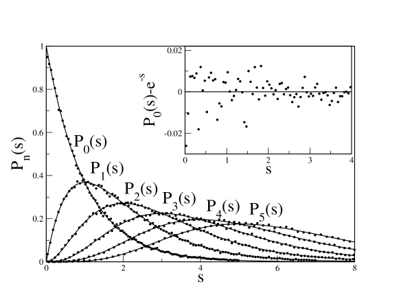
Figure 3: Nearest neighbour distributions for deterministic phases (19) with $k=50\,000.5$, $b=\pi$, $h=b/\sqrt{5}$, $a=2$, $d_{1}=1$, $d_{2}=1.5$. Solid lines are the Poisson predictions for these quantities (79). Insert: the difference between numerically calculated $P_{0}(s)$ and $\exp(-x)$.

Taken the random phase approximation as granted the unitary random matrix associated with the considered barrier billiards takes the form

$$B_{\mu,\nu}=e^{i\Phi_{\mu}}\frac{L_{\mu}L_{\nu}}{x_{\mu}+x_{\nu}},\qquad\mu,\nu=1,\ldots,N\ .$$ (80)

Quantities $L_{\mu}$ are, in general, complex numbers, $L_{\mu}=|L_{\mu}|e^{i\xi_{\nu}}$ whose moduli $|L_{\mu}|$ are related with $x_{\mu}$ by simple expressions (71) being merely a consequence of the unitarity. On the other hand, phases of $L_{\mu}$ are nontrivial and given by an infinite product as in Appendix A. By a conjugation phases of $L_{\nu}$ can be shifted to the first factor $L_{\mu}$ and now the total phase factor takes the form $\Phi_{\mu}^{\prime}=\Phi_{\mu}+2\xi_{\mu}$. As $\Phi_{\mu}$ are assumed to be independent random variables uniformly distributed at the unit circle the same will be valid for $\Phi_{\mu}^{\prime}$. These arguments establish that in the definition (80) coefficients $L_{\mu}$ can be considered as real numbers

$$L_{\mu}=\sqrt{2x_{\mu}\prod_{\nu\neq\mu}\frac{x_{\mu}+x_{\nu}}{x_{\mu}-x_{\nu}}}$$ (81)

provided that vector $\vec{x}$ obeys the intertwining conditions (72) and (73).

The random unitary matrix $B$ (80) depends on two groups of parameters. The first consists on $N$ independent random phases $\Phi_{m}$ uniformly distributed between $0$ and $2\pi$. The second includes $N$ coordinates $x_{\mu}$ obeying (72) and (73). To describe the barrier billiard indicated in figure 1 with irrational ratio $h/b$ vector $x_{\mu}$ has to chosen as indicated in (69) and when this ratio is rational and the exact modes are removed it has the form (75) or (77).

Though the $B$-matrix has been extracted from the exact quantisation of barrier billiards it remains meaningful for arbitrary coordinate sequence $x_{\mu}$ (obeying the above intertwining conditions).

The $B$-matrix (80) (as well as many other matrices with intermediate statistics) belongs to the so-called class of low complexity matrices complexity with a displacement operator of low rank displacement (cf., bogomolny ). The exact correlation functions for such matrices, in general, are unknown. It has been conjectured in toeplitz that nearest neighbour distributions for such matrices are well described by the normalised gamma-distributions

$$P_{n}(s)=a_{n}s^{\gamma_{n}}e^{-b_{n}s},\qquad\int_{0}^{\infty}P_{n}(s)ds=1,\qquad\int_{0}^{\infty}sP_{n}(s)ds=n+1$$ (82)

depended only on one parameter $\gamma_{n}$ which can be calculated as follows

$$\gamma_{n}=q_{n}-1$$ (83)

with $q_{n}$ equal the minimal number of parameters (co-dimension) needed to get exactly $n+2$ degenerated eigenvalues.

For Hermitian matrices the value of co-dimension is given by a theorem by von Neumann and Wigner and its generalisations neumann_wigner ; keller . For low complexity matrices and, in particular, for the $B$-matrix discussed above no exact results about $q_{n}$ are available (see toeplitz for ’physical’ determination of this quantity). It was argued in bogomolny that irrespective of the choice of coordinates $x_{\mu}$, the co-dimension $q_{n}$ for the unitary $B$-matrix equals $2n+2$ and, therefore, $\gamma_{n}=2n+1$. It means that the nearest neighbour distributions for random $B$-matrices should be well described by the following Wigner-type surmise

$$P_{n}(s)=\frac{2^{2n+2}}{(2n+1)!}s^{2n+1}e^{-2s}$$ (84)

which corresponds to the so-called semi-Poisson distribution plasma_model .

IV.3 Numerical calculations

To check these predictions numerical calculations of local spectral statistics for the above $B$-matrices with irrational and rational ratios $h/b$ were performed. Typical results are presented in figures 4, 5, and 6. The first figure shows 6 lowest nearest-neighbour distributions for the random $B$-matrix with $h/b=1/\sqrt{5}$, i.e., with $x_{\mu}$ given by (69) with $b=\pi$, $h=\pi/\sqrt{5}$, and $k=500.5$ which according to (68) leads to matrix dimension $N=999$. In the second figure the ratio $n/b$ was chosen equal to $1/3$ and the momentum $k=800.5$ which gives matrix dimension $N=1067$ (cf., (74)). In the third figure $h/b=2/5$ and $k=650.5$ which corresponds to $N=1040$ (see (78)). In all figures the results are averaged over $100$ realisations of random phases. It is clearly seen that simple semi-Poisson formulas (84) described quite well the numerical results.

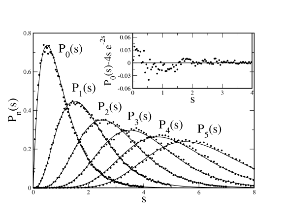
Figure 4: Nearest-neighbour distributions for random $N\times N$ $B$-matrices with irrational ratio $h=b/\sqrt{5}$ (black circles). In calculations $N=999$ corresponded to $k=500.5$, $b=\pi$, and $100$ realisations of random phases. Solid lines are the semi-Poisson formulas (84). Insert: the difference between numerically calculated $P_{0}(s)$ and the semi-Poisson prediction: $4se^{-2s}$.

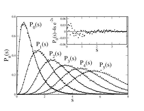
Figure 5: The same as in figure 4 but for ratio $h/b=1/3$, $k=800.5$, and $N=1067$.

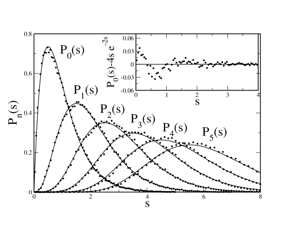
Figure 6: The same as in figure 4 but for ratio $h/b=2/5$, $k=650.5$, and $N=1040$.

V Summary

Barrier billiards are simple examples of pseudo-integrable systems with not-trivial and interesting classical and quantum properties. The main result of the paper is the construction of unitary random matrices associated with general barrier billiards. The principal importance of these matrices is that their spectral statistics is the same (up to a rescaling) as spectral statistics of two-dimensional barrier billiards.

To extract such random matrices from the exact quantum description of these billiards the following steps were done.

• Billiard boundaries perpendicular to the barrier were removed.

• The resulting problem corresponds to the scattering in an infinite slab with a half-plane inside.

• The exact $S$-matrix for this problem was calculated by the Wiener-Hopf method.

• In such a way one gets exact functions obeying both the Helmholtz equation and the correct boundary conditions on boundaries parallel to the barrier.

• Proper billiard eigenfunctions were written as linear combinations of these scattering waves with coefficients being obtained from boundary conditions on boundaries perpendicular to the barrier.

• The exact quantisation condition of barrier billiards appears in the form $\det(1+B(k))=0$ where the $B$-matrix differs from the $S$-matrix by phase factors depended on billiard dimensions parallel to the barrier.

• In the semiclassical limit two main simplifications occur:
  (i) $S$ and $B$ matrices become finite dimensional unitary matrices after ignoring exponentially small evanescent modes.
  (ii) The deterministic phases of propagating modes are substituted by independent random phases uniformly distributed on the unit circle.

The obtained $N\times N$ random unitary $B$-matrix depend on 2 groups of parameters: $N$ random phases and $N$ coordinates obeyed certain intertwining conditions. To describe barrier billiards coordinates have to be specially specified (see (69), (75), (77)) but the the $B$-matrix remains meaningful for an arbitrary choice of coordinates.

The spectral statistics of these $B$-matrices belongs to intermediate-type statistics which differs from both the Poisson statistics typical for integrable systems and the usual random matrix statistics characteristic for chaotic systems. Heuristic calculation of the Wigner-type surmise for these matrices reveals that their local spectral statistics is well described by the semi-Poisson distribution in a good agreement with numerical calculations. Further investigation of statistical properties of the $B$-matrices will be done elsewhere.

Applying these results to the barrier billiards leads to the following conclusions

• Local spectral correlation functions for rectangular billiards with a barrier inside as in figure 1(a) remain the same for (almost) all positions and heights of the barrier.

• These correlation functions are well described by the semi-Poisson distribution.

• The same should be also true for more general barrier billiards indicated in figure 1(b) with irrational ratio $h/b$. The case of these billiards with rational ratio $h/b$ requires a special investigation which is beyond the score of this paper.

Numerical calculations of spectral correlation functions were done so far only for symmetric barrier billiard wiersig ; gorin_wiersig and they are in agreement with the above statements. For more general barrier billiards discussed in the paper no numerics is known to the author. Analytical calculations of the spectral compressibility for general barrier billiards as in figure 1(a) with irrational ratio $d/a$ and $h/b=m/q$ with $m,q$ being co-prime integers were done in olivier_general . The result of this paper reads

$$K(0)=\frac{1}{2}+\frac{1}{q}$$ (85)

but in the calculations exact eigenstates discussed in Section III.5 were not removed. When these modes are put off the result is $K(0)=1/2$ private which coincides with the semi-Poisson prediction and corroborates the results of the paper.

Appendix A Factorisation of $K(\alpha)$

The purpose of this Appendix is to calculate the factorisation of the kernel $K(\alpha)$ into the product $K_{+}(\alpha)K_{-}(\alpha)$ needed in the application of the Wiener-Hopf method in Sections III and III.5.

For irrational ratio $h/b$ function $K(\alpha)$ (41) has the following form

$$K(\alpha)=\frac{\sin\big{(}q(\alpha)h\big{)}\sin\big{(}q(\alpha)(b-h)\big{)}}{bq(\alpha)\sin\big{(}q(\alpha)b\big{)}}$$ (86)

Each sinus function in this expression gives rise to the following series of zeros with integer $n\geq 1$ ($q(\alpha)=0$ is not a singular point)

$$q(\alpha^{(\beta)})=\frac{\pi n}{h_{\beta}},\qquad\alpha^{(\beta)}=\pm\sqrt{k^{2}-\frac{\pi^{2}n^{2}}{h_{\beta}^{2}}}\equiv\pm p_{n}^{(\beta)},\qquad\beta=1,2,3$$ (87)

where $h_{\beta}$ is the width of the corresponding channel given by (10).

Function $K_{+}(\alpha)$ has to be free of singularities in the upper half-plane of complex $\alpha$. Therefore it should include only negative zeros and poles. The needed factors can easily be calculated from the well-known formula

$$\sin x=x\prod_{n=1}^{\infty}\left(1-\frac{x^{2}}{\pi^{2}n^{2}}\right).$$ (88)

It is plain that

$$K_{+}(\alpha)=\frac{\sqrt{h(b-h)}}{b}\prod_{m=1}^{\infty}\frac{\Big{(}\sqrt{1-k^{2}b_{m}^{(2)2}}-i\alpha b_{m}^{(2)}\Big{)}\Big{(}\sqrt{1-k^{2}b_{m}^{(3)2}}-i\alpha b_{m}^{(3)}\Big{)}}{\Big{(}\sqrt{1-k^{2}b_{m}^{(1)2}}-i\alpha b_{m}^{(1)}\Big{)}}$$ (89)

where $b_{m}^{(\beta)}=h_{\beta}/(\pi m)$.

For the case $h/b=1/q$ considered in Section III.5 $b_{n}^{(3)}=b_{nq}^{(1)}$ and the infinite product in (89) contains only two factors

$$K_{+}^{\mathrm{res}}(\alpha)=\frac{\sqrt{h(b-h)}}{b}\frac{\prod_{m=1}^{\infty}\Big{(}\sqrt{1-k^{2}b_{m}^{(2)2}}-i\alpha b_{m}^{(2)}\Big{)}}{\prod_{\begin{subarray}{c}m=1\\ m\neq 0\mod q\end{subarray}}^{\infty}\Big{(}\sqrt{1-k^{2}b_{m}^{(1)2}}-i\alpha b_{m}^{(1)}\Big{)}}\,.$$ (90)

From general considerations the scattering $S$-matrix has to be unitary for propagating modes which implies the validity of (71). It is instructive to check this fact directly from the above formulas. The main step is the calculation $|K_{+}(p_{n}^{(\beta)})|^{2}$ for $\beta=1,2,3$. Even for propagating modes this function includes both the product of finite number of propagating modes with real momenta and the product of infinite number of evanescent modes which have pure imaginary momenta. Let us calculate them separately for each factor in (89) without explicitly bothering about the convergence.

Define

$$w^{(\beta)}(\alpha)=\prod_{m=1}^{\infty}\Big{(}\sqrt{1-k^{2}b_{m}^{(\beta)2}}-i\alpha b_{m}^{(\beta)}\Big{)},\qquad\beta=1,2,3\ .$$ (91)

One has for real $\alpha$ (with $N_{\beta}$ from (68))

$$w^{(\beta)}(\alpha)=\prod_{m=1}^{N_{\beta}}\Big{(}-i\sqrt{k^{2}b_{m}^{(\beta)2}-1}-i\alpha b_{n}^{(\beta)}\Big{)}\prod_{m=N_{\beta}+1}^{\infty}\Big{(}\sqrt{1-k^{2}b_{m}^{(\beta)2}}-i\alpha b_{m}^{(\beta)}\Big{)}\,.$$ (92)

Therefore

$$\Big{|}w^{(\beta)}(\alpha)\Big{|}^{2}=\prod_{m=1}^{N_{\beta}}b_{m}^{(\beta)2}\Big{(}\alpha+p_{m}^{(\beta)}\Big{)}^{2}\prod_{m=N_{\beta}+1}^{\infty}\Big{(}1-(k^{2}-\alpha^{2})b_{m}^{(\beta)2}\Big{)}\,.$$ (93)

Assume that $\alpha=p_{n}^{(l)}$ with $l\neq\beta$. Then the second product is not zero for all $m$ and one gets

$$\Big{|}w^{(\beta)}(p_{n}^{(l)})\Big{|}^{2}=\prod_{m=1}^{N_{\beta}}b_{m}^{(\beta)2}\frac{\Big{(}p_{n}^{(l)}+p_{m}^{(\beta)}\Big{)}^{2}}{\Big{(}1-(h_{\beta}n)^{2}/(h_{l}m)^{2}\Big{)}}\prod_{m=1}^{\infty}\Big{(}1-\frac{h_{\beta}^{2}n^{2}}{h_{l}^{2}m^{2}}\Big{)}\,.$$ (94)

Using the fact that $1-(h_{\beta}n)^{2}/(h_{l}m)^{2}=b_{m}^{(\beta)2}\big{(}p_{n}^{(l)2}-p_{m}^{(\beta)2}\big{)}$ and taking into account (88) one gets that

$$\Big{|}w^{(\beta)}(p_{n}^{(l)})\Big{|}^{2}=\frac{h_{l}\sin(\pi h_{\beta}n/h_{l})}{\pi h_{\beta}n}\prod_{m=1}^{N_{\beta}}\frac{p_{n}^{(l)}+p_{m}^{(\beta)}}{p_{n}^{(l)}-p_{m}^{(\beta)}},\qquad l\neq\beta\,.$$ (95)

For $l=\beta$ this transformation does not work as the second product in (94) is zero for $m=n$. This formal difficulty can easily be avoid by the following manipulation (taking into account that $n$ is from a propagating mode and $m$ is the second product is from an evanescent mode)

$$\prod_{m=N_{\beta}+1}^{\infty}\Big{(}1-\frac{n^{2}}{m^{2}}\Big{)}=\frac{\prod_{m=1,\ m\neq n}^{\infty}\Big{(}1-\frac{n^{2}}{m^{2}}\Big{)}}{\prod_{m=1,\ m\neq n}^{N_{\beta}}\Big{(}1-\frac{n^{2}}{m^{2}}\Big{)}}\,.$$ (96)

The calculation of the numerator is performed as follows

$$\prod_{m=1,\ m\neq n}^{\infty}\Big{(}1-\frac{n^{2}}{m^{2}}\Big{)}=\lim_{x\to n}\frac{1}{1-x^{2}/n^{2}}\prod_{m=1}^{\infty}\Big{(}1-\frac{x^{2}}{m^{2}}\Big{)}=\lim_{x\to n}\frac{\sin\pi x}{\pi x(1-x^{2}/n^{2})}=-\frac{1}{2}(-1)^{n}\,.$$ (97)

Therefore

$$\Big{|}w^{(\beta)}(p_{n}^{(\beta)})\Big{|}^{2}=\frac{2(-1)^{n+1}p_{n}^{(\beta)2}h_{\beta}^{2}}{\pi^{2}n^{2}}\prod_{m=1,\ m\neq n}^{N_{\beta}}\frac{p_{n}^{(\beta)}+p_{m}^{(\beta)}}{p_{n}^{(\beta)}-p_{m}^{(\beta)}}\,.$$ (98)

Finally one finds that

$$\Big{|}K_{+}(p_{n}^{(1)})\Big{|}^{2} = \frac{\sin^{2}(\pi hn/b)}{2b^{2}p_{n}^{(1)2}}\prod_{m=1,\ m\neq n}^{N_{1}}\frac{p_{n}^{(1)}-p_{m}^{(1)}}{p_{n}^{(1)}+p_{m}^{(1)}}\prod_{m=1}^{N_{2}}\frac{p_{n}^{(1)}+p_{m}^{(2)}}{p_{n}^{(1)}-p_{m}^{(2)}}\prod_{m=1}^{N_{3}}\frac{p_{n}^{(1)}+p_{m}^{(3)}}{p_{n}^{(1)}-p_{m}^{(3)}}\,,$$ (99)

$$\Big{|}K_{+}(p_{n}^{(2)})\Big{|}^{2} = -\frac{2(b-h)^{3}p_{n}^{(2)2}}{b\pi^{2}n^{2}}\prod_{m=1}^{N_{1}}\frac{p_{n}^{(2)}-p_{m}^{(1)}}{p_{n}^{(2)}+p_{m}^{(1)}}\prod_{m=1,\ m\neq n}^{N_{2}}\frac{p_{n}^{(2)}+p_{m}^{(2)}}{p_{n}^{(2)}-p_{m}^{(2)}}\prod_{m=1}^{N_{3}}\frac{p_{n}^{(2)}+p_{m}^{(3)}}{p_{n}^{(2)}-p_{m}^{(3)}}\,,$$ (100)

$$\Big{|}K_{+}(p_{n}^{(3)})\Big{|}^{2} = -\frac{2h^{3}p_{n}^{(3)2}}{b\pi^{2}n^{2}}\prod_{m=1}^{N_{1}}\frac{p_{n}^{(3)}-p_{m}^{(1)}}{p_{n}^{(3)}+p_{m}^{(1)}}\prod_{m=1}^{N_{2}}\frac{p_{n}^{(3)}+p_{m}^{(2)}}{p_{n}^{(3)}-p_{m}^{(2)}}\prod_{m=1,\ m\neq n}^{N_{3}}\frac{p_{n}^{(3)}+p_{m}^{(3)}}{p_{n}^{(3)}-p_{m}^{(3)}}\,.$$ (101)

Taking into account (58) it is plain that the relations (71) implying the unitarity are fulfilled.

References

- (1) E. Gutkin, Billiards in polygons, Physica D 19, 311 (1986); E. Gutkin, Billiards in polygons: survey of recent results, J. Stat. Phys.83, 7 (1996).
- (2) P.J. Richens and M.V. Berry, Pseudointegrable systems in classical and quantum mechanics, Physica D: Nonlinear Phenomena 2, 495 (1981).
- (3) A.N. Zemlyakov and A.B. Katok, Topological transitivity in billiards in polygons, Math. Notes 18, 760 (1975).
- (4) M. V. Berry and M. Tabor, Level clustering in the regular spectrum, Proc. R. Soc. Lond. A 356, 375, (1977).
- (5) O. Bohigas, M. J. Giannoni, and C. Schmit, Characterization of chaotic quantum spectra and universality of level fluctuation laws, Phys. Rev. Lett. 52, 1 (1984).
- (6) T. Cheon and T. D. Cohen, Quantum level statistics of pseudointegrable billiards, Phys. Rev. Lett. 62, 2769 (1989).
- (7) A. Shudo and Y. Shimizu, Extensive numerical study of spectral statistics for rational and irrational polygonal billiards, Phys. Rev. E 47, 54 (1993).
- (8) A. Shudo, Y. Shimizu, Petr S̆eba, J. Stein, H.-J. Stöckmann, and K. Zyczkowski, Statistical properties of spectra of pseudointegrable systems, Phys. Rev. E 49, 3748 (1994).
- (9) H. C. Schachner, G. M. Obermair, Quantum billiards in the shape of right triangles, Z. Physik B - Condensed Matter 95, 113 (1994).
- (10) E. Bogomolny, U. Gerland, and C. Schmit, Models of intermediate spectral statistics, Phys. Rev.E 59, R1315 (1999).
- (11) E. Bogomolny, U. Gerland, and C. Schmit, Short-range plasma model for intermediate spectral statistics, Eur. Phys. J. B 19, 121 (2001).
- (12) B. Grémaud and S. R. Jain, Spacing distributions for rhombus billiards, J. Phys. A: Math. Gen. 31, L637 (1998).
- (13) T. Gorin, Generic spectral properties of right triangle billiards, J. Phys. A: Math. Gen. 34, 8281 (2001).
- (14) J. Wiersig, Spectral properties of quantized barrier billiards, Phys. Rev. E 65, 046217 (2002).
- (15) T. Gorin and J. Wiersig, Low rank perturbations and the spectral statistics of pseudointegrable billiards, Phys. Rev. E 68, 065205 (2003).
- (16) B. L. Altshuler, I. Kh. Zharekeshev, S. A. Kotochigava, and B.I. Shklovskii, Repulsion between levels and the metal-insulator transition, Sov. Phys. JETP 67, 625 (1988).
- (17) B.I. Shklovskii, B. Shapiro, B.R. Sears, P. Lambrianides, and H.B. Shore, Statistics of spectra ofdisordered systems near the metal-insulator transition, Phys. Rev. B 47, 11487 (1993).
- (18) E. Bogomolny, Barrier billiard and random matrices, arXiv:2107.03364 (2021).
- (19) E. Bogomolny, Semiclassical quantization of multidimensional systems, Nonlinearity 5, 805, (1992).
- (20) E. Doron and U. Smilansky, Semiclassical quantization of chaotic billiards: a scattering theory approach, Nonlinearity 5, 1055 (1992).
- (21) B. Noble, Methods based on the Wiener-Hopf technique, Chelsea Publishing Company, New York, N. Y. (1988).
- (22) J. Marklof, Spectral form factors of rectangle billiards, Comm. Math. Phys. 199, 169 (1998).
- (23) V. Y. Pan, Z. Q. Chen, and A. Zheng, The complexity of the algebraic eigenproblem, STOC ’99, Proc. of the thirty-first annual ACM symposium on theory of computing, 507 (1999).
- (24) T. Kailath, S.-Y. Kung, and M. Morf, Displacement ranks of matrices and linear equations, J. Math. Anal. Applic. 68, 395 (1979).
- (25) E. Bogomolny and O. Giraud, Statistical properties of structured random matrices, Phys. Rev. E 103, 042213 (2021).
- (26) J. von Neumann and E. P. Wigner, Uber das Verhalten von Eigenwerten bei adiabatischen Prozessen, Phys. Z. 30, 467 (1929).
- (27) J. B. Keller, Multiple eigenvalues, Lin. Alg. Appl. 429, 2209 (2008).
- (28) O.Giraud, Periodic orbits and semiclassical form factor in barrier billiards, Commun. Math. Phys. 260, 183 (2005).
- (29) O. Giraud, private communication (2021).