M2MRF: Many-to-Many Reassembly of Features for Tiny Lesion Segmentation in Fundus Images

Abstract

Feature reassembly is an essential component in modern CNN-based segmentation approaches, which includes feature downsampling and upsampling operators. Existing operators reassemble multiple features from a small predefined region into one for each target location independently. This may result in loss of spatial information, which could vanish activations caused by tiny lesions particularly when they cluster together. In this paper, we propose a many-to-many reassembly of features (M2MRF). It reassembles features in a dimension-reduced feature space and simultaneously aggregates multiple features inside a large predefined region into multiple target features. In this way, long range spatial dependencies are captured to maintain activations on tiny lesions. Experimental results on two lesion segmentation benchmarks, i.e. DDR and IDRiD, show that (1) our M2MRF outperforms existing feature reassembly operators; (2) equipped with our M2MRF, the HRNetv2 is able to achieve significant better performance to CNN-based segmentation methods and competitive even better performance to two recent transformer-based segmentation methods. Our code is made publicly available at https://github.com/CVIU-CSU/M2MRF-Lesion-Segmentation.

Introduction

This paper focuses on segmentation of tiny lesions, e.g. soft exudates (SEs), hard exudates (EXs), microaneurysms (MAs) and hemorrhages (HEs) (see Fig. 1) in colour fundus images, which is an important prerequisite for enabling computers to assist human doctors for clinical purpose. It falls into the research area of semantic segmentation.

With the rise of deep convolutional neural networks (CNN), many CNN-based approaches such as (Long, Shelhamer, and Darrell 2015; Ronneberger, Fischer, and Brox 2015; Xie and Tu 2015; Chen et al. 2017; Zhao et al. 2017; Chen et al. 2018; Wang et al. 2020) have been proposed for semantic segmentation and achieved extraordinary progress. On Cityscapes (Cordts et al. 2016) with 19 classes, the mean of class-wise intersection over union (mIoU) by a state-of-the-art approach HRNetV2 (Wang et al. 2020) has been improved to 81%. However, when fine-tuning HRNetV2 (Wang et al. 2020) for four-class lesion segmentation in fundus images, the mIoU on IDRiD (Porwal et al. 2020) decreases to 47%. Why is lesion segmentation so much harder than natural scene image segmentation?

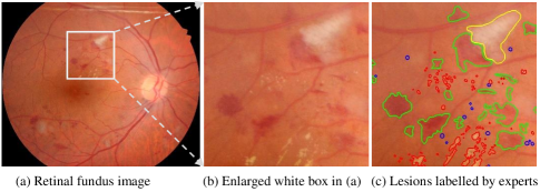
Figure 1: Example for colour fundus images and lesions. Four types of lesions i.e. SEs, EXs, MAs and HEs are delineated in yellow, red, blue and green respectively. Many lesions are extremely small and the size variance across them are enormous

Two possible factors behind performance gap are the extreme small size of lesions and large scale variation across them. Interestingly, almost 50% lesions are less than 256 pixels in images of size $4288\times 2848$ from IDRiD (Porwal et al. 2020) dataset provided by the 2018 ISBI grand challenge. Such tiny size of lesions rises an extreme challenge for CNN-based segmentation approaches to learn discriminative representations with enough spatial information. To make matters worse, the smallest 10% lesions in IDRiD (Porwal et al. 2020) only contain less than 74 pixels while the largest 10% lesions contain more than 1920 pixels. Tiny lesions require CNNs maintain as enough local information as possible within a small receptive field while large lesions require CNNs exploit long range contexts over a large receptive field. This demand contradiction raised by enormous size variation presents another challenge for CNN-based approaches. Moreover, in fundus images, multiple lesions with large size variation always coexist and cluster together, which makes the representation learning more challenge.

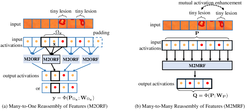
Figure 2: Illustration of our motivation. Here we take the downsampling with rate of 2 for example. Input contains two EXs, which are delineated with red lines. Feature activations mainly caused by background and EXs are represented by circles in light orange and red respectively. With the input activations, we want to preserve activations of both EXs. To generate activation $\mathbf{y}$, M2ORF first finds the source feature $\mathbf{x}$ in input activations, and then determines a small local region $\Omega_{\mathbf{x}}$ centred on $\mathbf{x}$, and finally reassembles features inside $\Omega_{\mathbf{x}}$ with importance weighting kernel $\mathbf{W}_{\Omega_{\mathbf{x}}}$ into target activation $\mathbf{y}$, as illustrated in (a). M2ORF ignores the coexist of multiple lesions, which may vanish tiny lesion activations. Instead, our M2MRF directly learns to reassemble activations inside a large local region $\mathbf{P}$ to generate multiple output activations $\mathbf{Q}$ simultaneously which enables subtle activations be enhanced mutually and well preserved, as illustrated in (b). Here $\mathbf{W}_{\mathbf{P}}$ is the importance weighting kernel in M2MRF.

Taking an in-depth look at modern CNN-based segmentation approaches (Long, Shelhamer, and Darrell 2015; Ronneberger, Fischer, and Brox 2015; Xie and Tu 2015; Chen et al. 2017; Zhao et al. 2017; Chen et al. 2018; Sun et al. 2019; Wang et al. 2020), the challenges of applying them to lesion segmentation are mainly caused by the repetitive utilisation of operators for reassembly of features (RF operators for short), i.e. downsampling and upsampling operators. Downsampling operator is the key contributor to enlarge CNNs’ receptive fields via reducing the spatial resolution of feature maps (Chen et al. 2017; Gao, Wang, and Wu 2019). Conversely, upsampling operator is essential to recover the spatial resolution for better segmentation. Strided max-pooling and strided convolution (Springenberg et al. 2015; Sun et al. 2019; Wang et al. 2020) are two widely-adopted operators for downsampling while bilinear interpolation and deconvolution (Zeiler et al. 2010)(Zeiler and Fergus 2014; Long, Shelhamer, and Darrell 2015; Noh, Hong, and Han 2015) are two common choices for feature upsampling. Those RF operators assume that features in target feature map are independent of each other and follow a many-to-one pipeline. They first determine a small local region in input feature map, according to a target location in output feature map. Then, they reassemble multiple features in the small local region with importance weighting kernels into one as the output feature for the target location. However, during the downsampling process, resembling features inside small local region independently for each target location ignores the coexist of multiple tiny lesions and limits ability to capture long-range dependencies for mutual activation enhancement between tiny lesions. These further lead to dilution or even vanishing of subtle activations caused by tiny lesions (Gao, Wang, and Wu 2019), as illustrated in Fig. 2 (a). Once subtle lesion activations are vanished, it is almost impossible to recover them via upsampling, which consequently results in miss identification.

In this paper, we aim to address above issues raised by M2ORF operators within the context of tiny lesion segmentation. Basically, we pursue a RF operator that is capable of 1) preserving subtle activations caused by tiny lesions; 2) easily being integrated into existing CNN-based segmentation models. To this end, we propose a lightweight RF operator, termed as Many-to-Many Reassembly of Features (M2MRF), which considers the coexist of tiny lesions and enhances their subtle activations mutually via reassembling multiple features inside a large predefined region into multiple target features simultaneously (see Fig.2(b)). We demonstrate the effectiveness of our M2MRF on two public tiny lesion segmentation datasets, i.e. DDR (Li et al. 2019) and IDRiD (Porwal et al. 2020). Experiments show that our M2MRF outperforms state-of-the-art RF operators. Particularly, compared with a strong segmentation baseline HRNetv2 (Wang et al. 2020), our M2MRF exhibits significant improvements with negligible increase of parameters and inference time.

The rest of this paper is organised as follows. The most related works are briefly reviewed in Section Related Work, and our proposed M2MRF and its application on tiny lesion segmentation are described in Section Method. Section Experiments and Discussions presents the experiments and analysis. The conclusion is presented in Section Conclusion.

Related Work

Feature reassembly operators in deep networks. In existing deep networks (Long, Shelhamer, and Darrell 2015) (Ronneberger, Fischer, and Brox 2015) (Chen et al. 2017) (Chen et al. 2018) (Wang et al. 2020) (Sun et al. 2019) (Noh, Hong, and Han 2015) (Badrinarayanan, Kendall, and Cipolla 2017), strided max-pooling (LeCun et al. 1990) and strided convolution are two widely-adopted operators for feature downsampling. Bilinear interpolation, deconvolution and unpooling(Zeiler and Fergus 2014) (Zeiler, Taylor, and Fergus 2011) are widely-adopted for feature upsampling. The general idea of these operators is to generate a feature vector for each target location via reassembling multiple features inside a predefined region with importance kernels. Particularly, importance kernels for strided max-pooling, unpooling and bilinear interpolation are hand-crafted and feature maps are processed channel-by-channel efficiently. However, they ignore the context dependencies across channels and the diversity of local patterns. Instead, the importance kernels for strided convolution and deconvolution are learned. Their dimension depends on the input features, which is always high in CNNs. This makes the computation burden of reassembly heavy when large importance kernels are used. Thus it is difficult to reassemble features from a large region.

Recently, novel ideas about learning-based RF operators emerge. LIP (Gao, Wang, and Wu 2019) learns adaptive importance kernels based on inputs to enhance the discriminative features. In CARAFE (Wang et al. 2019) and CARAFE++ (Wang et al. 2021a), content-aware kernels for each target position is learned according to input features for feature reassembly. Similarly, IndexNet (Lu et al. 2019) (Lu et al. 2020) learns importance kernels from feature encoder to guide the feature reassembly in both feature encoder and decoder. Instead of reassembling features inside a predefined region, deformable RoI pooling (Dai et al. 2017) reassembles features in an adaptive region which is learned from the input features. To model the affinity information, A²U (Dai, Lu, and Shen 2021) is proposed to learn importance kernels according to second-order features for feature reassembly. However, these learning-based operators still follow the paradigm of many-to-one feature reassembly and are prone to dilute or even vanish features of tiny lesions.

Tiny lesion segmentation in fundus images. The development originated from one-type lesion segmentation with either hand-crafted features (Zhang et al. 2014; Liu et al. 2017; Du et al. 2020) or deep features (Liu et al. 2021a) and has been evolved to multi-type lesion segmentation. For example, in (Li et al. 2019), PSPNet (Zhao et al. 2017) and DeeplabV3+ (Chen et al. 2018) are directly fine-tuned for multi-type lesion segmentation. Guo et al. (Guo et al. 2019) develop a network named L-Seg on the top of FCN (Long, Shelhamer, and Darrell 2015). More recently, multi-task learning frameworks (Foo et al. 2020)(Wang et al. 2021b) are proposed to exploit the correlation among tasks of lesion segmentation and others to boost performance of all tasks. All of those methods adopt many-to-one RF operators during feature encoding and decoding and are prone to ignore tiny lesions. In (Sun et al. 2021), specially designed lesion filters are proposed to discover lesions and suspicious lesion regions are detected. However, this work is unable to provide fine lesion regions and predict lesion classes. One thing worth to mention is that the public datasets with pixel-level annotations also updates from one-type lesion segmentation e.g. E-ophtha EX (Decenciere et al. 2013) and e-ophtha MA (Decenciere et al. 2013) to multi-type lesion segmentation e.g. IDRiD (Porwal et al. 2020) and DDR (Li et al. 2019).

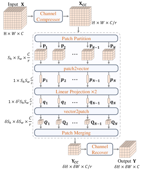
Figure 3: An overview of our Many-to-Many Reassembly of Features (M2MRF). $\{\mathbf{P}_{l}\}_{l=1}^{L}$ and $\{\mathbf{Q}_{l}\}_{l=1}^{L}$ are feature patches of size $S_{h}\times S_{w}\times\frac{C}{r}$ and $\delta S_{h}\times\delta S_{w}\times\frac{C}{r}$ respectively, where $L(=\lceil H/S_{h}\rceil\cdot\lceil W/S_{w}\rceil)$ is the number of patches. $\{\mathbf{p}_{l}\}_{l=1}^{L}$ and $\{\mathbf{q}_{l}\}_{l=1}^{L}$ are feature vectors. In this figure, a feature map of size $H\times W\times C$ is downsampled by a factor of $\delta(=1/2)$. (Best view in colour)

Deep semantic segmentation. The development can be mainly classified into three veins. The first vein focuses on how to produce and aggregate multi-scale representations. FCN (Long, Shelhamer, and Darrell 2015) provides a natural solution which reuses middle-level features to compensate for spatial details in high-level features. UNet (Ronneberger, Fischer, and Brox 2015) propagates low-level information to high-levels via skip connections, which also inspires many variants specially for medical image segmentation such as VNet (Milletari, Navab, and Ahmadi 2016), UNet++ (Zhou et al. 2019), MNet (Fu et al. 2018) and SAN (Liu et al. 2019). In (Li et al. 2020), gated fully fusion is proposed to selectively fuse multi-level features. The second vein focuses on high-resolution representation learning. For example, in (Ronneberger, Fischer, and Brox 2015; Noh, Hong, and Han 2015; Badrinarayanan, Kendall, and Cipolla 2017), an encoder-decoder architectural style is adopted to gradually recover feature resolution while HRNet (Sun et al. 2019; Wang et al. 2020) is specially designed to learn high-resolution representations. The third vein introduces attention mechanism and variant modules such as DANet (Fu et al. 2019), DRANet (Fu et al. 2020), CCNet (Huang et al. 2019), RecoNet (Chen et al. 2020), HANet (Choi, Kim, and Choo 2020) and DNL (Yin et al. 2020) are developed to explore long range dependencies. More recently, vision transformers such as Swin (Liu et al. 2021b), Twins (Chu et al. 2021) and CSWin (Dong et al. 2021) are developed for segmentation. However, those methods are designed for segmenting objects in proper size rather than tiny size.

Method

In this section, we first give a simple analysis for M2ORF operators and then detail our M2MRF. Finally we take HRNetV2 (Wang et al. 2020) as an example and present how to integrate our M2MRF into CNN-architectures for tiny lesion segmentation.

Analysis for M2ORF Operators

Given the input feature map $\mathbf{X}\in\mathcal{R}^{H\times W\times C}$ and sample rate $\delta$ where $\delta>0$, the goal of feature reassembly is to generate target feature map $\mathbf{Y}\in\mathcal{R}^{\lfloor\delta H\rfloor\times\lfloor\delta W\rfloor\times C}$ via finding a function mapping $\Phi$ parametrised by importance kernels $\mathbf{W}$:

$$\mathbf{Y}=\Phi(\mathbf{X};\mathbf{W})\;.$$ (1)

Here $\delta<1$ for downsampling and $\delta>1$ for upsampling.

To make the feature reassembly computational efficient, most existing methods degrade it to a many-to-one local sampling problem, i.e. reassembling multiple features in a predefined local region to one target feature. Specifically, for any target feature $\mathbf{y}\in\mathcal{R}^{C}$ at location $(i^{\prime},j^{\prime})$ in $\mathbf{Y}$, most existing methods assume that there is a corresponding source feature $\mathbf{x}\in\mathcal{R}^{C}$ at location $(i,j)$ in $\mathbf{X}$, where $i=\lfloor i^{\prime}/\delta\rfloor$ and $j=\lfloor j^{\prime}/\delta\rfloor$. They follow three steps to obtain $\mathbf{y}$ : (1) setting/learning a local region $\Omega_{\mathbf{x}}$ according to $\mathbf{x}\in\mathcal{R}^{C}$; (2) with $\Omega_{\mathbf{x}}$, setting/learning corresponding importance kernels $\mathbf{W}_{i^{\prime},j^{\prime}}$; (3) obtaining $\mathbf{y}$ via

$$\mathbf{y}=\Phi(\mathbf{P}_{\Omega_{\mathbf{x}}};\mathbf{W}_{i^{\prime},j^{\prime}})\;,$$ (2)

where $\mathbf{P}_{\Omega_{\mathbf{x}}}$ denotes features in $\Omega_{\mathbf{x}}$.

Obviously, M2ORF operators assume that each target feature in $\mathbf{Y}$ is independent and ignores the coexist of multiple lesions. Additionally, considering the computational efficiency, previous RF operators such as strided convolution, deconvolution, CARAFE++ (Wang et al. 2021a) and A²U (Dai, Lu, and Shen 2021) usually consider a small size $\Omega_{\mathbf{x}}$, which makes them fail to exploit long-range dependencies. As a result, activations caused by tiny lesions are prone to be diluted or even vanished. To alleviate the dilution of tiny lesion activations, one natural solution is to discard the assumption of M2ORF and generate multiple features for multiple target locations with features inside a large local region simultaneously. To this end, we propose many-to-many reassembly of features (M2MRF).

Many-to-Many Reassembly of Features

Module overview. Fig. 3 illustrates an overview of reassembling the input feature map $\mathbf{X}$ of size $H\times W\times C$ with our M2MRF operator with sample rate $\delta$ to feature map $\mathbf{Y}$ of size $\lfloor\delta H\rfloor\times\lfloor\delta W\rfloor\times C$. First, a channel compressor is performed on $\mathbf{X}$ to reduce its channel from $C$ to $\frac{C}{r}$ for computational efficiency. We denote the output as $\mathbf{X}_{CC}$. Then we partition $\mathbf{X}_{CC}$ into feature patches $\{\mathbf{P}_{l}\}_{l=1}^{L}$ of size $S_{h}\times S_{w}\times\frac{C}{r}$, where $L=\lfloor H/S_{h}\rfloor\cdot\lfloor W/S_{w}\rfloor$. Our proposed M2MRF is performed on each feature patch and outputs $\{\mathbf{Q}_{l}\}_{l=1}^{L}$ of size $\lfloor\delta H\rfloor\times\lfloor\delta W\rfloor\times\frac{C}{r}$. Thereafter, those patches are merged into feature map $\mathbf{Y}_{CC}$ of size $\lfloor\delta H\rfloor\times\lfloor\delta W\rfloor\times\frac{C}{r}$. Finally, we recover the feature channel to $C$ via channel recover. For channel compressor and recover, we simply implement them with a $1\times 1$ regular convolution layer.

M2MRF. With a local feature patch $\mathbf{P}\in\{\mathbf{P}_{l}\}_{l=1}^{L}$, the goal is to generate $\mathbf{Q}$ of size $\lfloor\delta S_{h}\rfloor\times\lfloor\delta S_{w}\rfloor\times\frac{C}{r}$:

$$\mathbf{Q}=\Phi(\mathbf{P};\mathbf{W}_{patch})\;.$$ (3)

Here we let $M=\lfloor\delta S_{h}\rfloor\times\lfloor\delta S_{w}\rfloor,N=S_{h}\times S_{w}$, and treat this task as generating $M$ features $\mathbf{Q}=\{\mathbf{y}_{m}\}_{m=1}^{M}$ from $N$ source features $\mathbf{P}=\{\mathbf{x}_{n}\}_{n=1}^{N}$ where $\mathbf{y}_{m}$, $\mathbf{x}_{n}\in\mathcal{R}^{1\times\frac{C}{r}}$. To achieve this, one option is to adopt linear projection, thus Eq.(3) can be expressed as:

$$[\mathbf{y}_{1},\cdots,\mathbf{y}_{M}]=[\mathbf{x}_{1},\cdots,\mathbf{x}_{N}][\mathbf{W}_{1},\cdots,\mathbf{W}_{M}]\;,$$ (4)

where $\mathbf{W}_{1},\cdots,\mathbf{W}_{M}$ are parameters of size $\frac{NC}{r}\times\frac{C}{r}$ to be learned. Therefore we have $\mathbf{W}_{patch}=[\mathbf{W}_{1},\cdots,\mathbf{W}_{M}]$ whose size is $\frac{NC}{r}\times\frac{MC}{r}$. For simplicity, we denote $\mathbf{p}=[\mathbf{x}_{1},\cdots,\mathbf{x}_{N}],\mathbf{q}=[\mathbf{y}_{1},\cdots,\mathbf{y}_{M}]$, and rewrite Eq.(4) as:

$$\mathbf{q}=\mathbf{p}\mathbf{W}_{patch}\;.$$ (5)

To make use of long-range dependencies, $S_{h}S_{w}$ is required to be large. Accordingly, $N$ and $M$ are large and $\mathbf{W}_{patch}$ would be a large matrix. On one hand, it is always difficult to optimise such a large matrix. On the other hand, storing a large matrix results in high memory consumption. To reduce the number of parameters to be learned, we decompose $\mathbf{W}_{patch}$ to two small matrices via a two-layer linear projections. Thus Eq. (4) can be rewrote as:

$$\mathbf{q}=(\mathbf{p}\mathbf{W}_{patch}^{\prime})\mathbf{W}_{patch}^{\prime\prime}\;,$$ (6)

where $\mathbf{W}_{p}^{\prime}\in\mathcal{R}^{\frac{NC}{r}\times\frac{NC}{\alpha r}}$ and $\mathbf{W}_{p}^{\prime\prime}\in\mathcal{R}^{\frac{NC}{\alpha r}\times\frac{MC}{r}}$ are parameters in the two linear projections, and $\alpha\geq 1$ such that the matrix dimension of $\mathbf{W}_{patch}^{\prime}$ and $\mathbf{W}_{patch}^{\prime\prime}$ is less than $\mathbf{W}_{patch}$ far away.

Figure 4: Two variants of our M2MRF. Here we take $\delta=4$ for upsampling and $\delta=1/4$ for downsampling as examples.

M2MRF for Tiny Lesion Segmentation

As HRNetV2 (Wang et al. 2020) is originally designed for high-resolution representation learning and has achieved state-of-the-art performance on semantic segmentation task, we adopt it as the baseline for tiny lesion segmentation. In HRNetV2 (Wang et al. 2020), RF operators involve in the fusion module to exchange information across multi-resolution feature maps. Strided convolution with stride of 2 is adopted for downsampling and bilinear interpolation for upsampling. Repeating $t$ times of the strided convolution, the feature resolution decreases to $1/2^{t}$. To build M2MRF variants, we replace the repeated strided convolution and bilinear interpolation with our M2MRF.

We propose two options to replace the repeated $t$ layers of strided convolution with our M2MRF. One is to replace each strided convolution layer with our proposed M2MRF with $\delta=1/2$ to gradually decrease the feature resolution. We term it as cascade M2MRF. The other is to directly set $\delta$ to $1/2^{t}$ in M2MRF to replace the entirety of $t$ layers of strided convolution. We term it as one-step M2MRF. Similarly, there are also two options to replace bilinear interpolation layer with scale factor $2^{t}$. One is to cascade M2MRF with $\delta=2$ to gradually increase the feature resolution to $2^{t}$. The other is one-step M2MRF with $\delta=2^{t}$ which directly increases the feature resolution to $2^{t}$. Taking $t=2$ for example, Fig.4 illustrates the cascade M2MRF and one-step M2MRF for downsampling and upsampling respectively.

With high-resolution feature maps by variants of HRNetV2 equipped with our M2MRFs, we attach multiple binary classifiers on them to obtain probability maps for each lesion class. Considering the extremely class imbalance in tiny lesion segmentation, we adopt Dice loss (Milletari, Navab, and Ahmadi 2016) to train M2MRF-HRNetV2 as well as the baseline.

Experiments and Discussions

To validate the effectiveness of our M2MRF module on tiny lesion segmentation, we carry out experiments on two public datasets i.e. DDR (Li et al. 2019) and IDRiD (Porwal et al. 2020). For evaluation metrics, we follow (Porwal et al. 2020) and utilize Area Under Precision-Recall curve (AUPR). We also report mean F-score (mF) and mean IoU (mIoU) as they are widely adopted for segmentation evaluation.

Implementation Details

Datasets and augmentation

DDR (Li et al. 2019) contains 757 colour fundus images of size ranging from $1088\times 1920$ to $3456\times 5184$, among which 383 for training, 149 for validation and $225$ for testing. In DDR (Li et al. 2019), 24154, 13035, 1354 and 10563 connected regions are annotated by experts as EXs, HEs, SEs and MAs respectively. To our best knowledge, DDR (Li et al. 2019) is the largest dataset for lesion segmentation in fundus images. IDRiD (Porwal et al. 2020) contains 81 colour fundus images of size $4288\times 2848$ among which 54 for training and 27 for testing. It is provided by a grand challenge on “Diabetic Retinopathy – Segmentation and Grading” in 2018. In IDRiD (Porwal et al. 2020), 11716, 1903, 150 and 3505 connected regions are annotated by experts as EXs, HEs, SEs and MAs respectively.

Before feeding images into models, we follow (Wang et al. 2021b) and downsample images in DDR (Li et al. 2019) such that the long side is 1024. Thereafter, zero padding is used on short side to enlarge its length to 1024. Following (Liu et al. 2021a; Guo et al. 2019), images in IDRiD (Porwal et al. 2020) are resized to $1440\times 960$. Three tricks are adopted to augment the training data: multi-scale (0.5-2.0), rotation (90^∘, 180^∘ and 270^∘) and flipping(horizontal and vertical).

Experimental setting

M2MRF-HRNetV2 is built on the top of implementation of HRNetV2 (Wang et al. 2020) provided by MMSegmentation (Contributors 2020). We initialize parameters associated with both M2MRF and dense classification layers with Gaussian distribution with zeros mean and standard deviation of 0.01 and the rest with the pre-trained model on ImageNet (Krizhevsky, Sutskever, and Hinton 2012). SGD is used for parameters optimisation. Hyper-parameters include: initial learning rate (0.01 poly policy with power of 0.9), weight decay (0.0005), momentum (0.9), batch size (4) and iteration epoch (60k on DDR and 40k on IDRiD).

Results on DDR and Analysis

Ablation study for M2MRF

There are four hyper-parameters in our M2MRF, i.e. the patch size $S_{h}$ and $S_{w}$, $r$ in channel compressor, $\alpha$ in Eq.(6). For $S_{h}$ and $S_{w}$, we directly let them equal and conduct experiments with setting $\{4,8,16\}$. For $r$ and $\alpha$, we conduct experiments with setting $r$ to $\{2,4,8\}$ and $\alpha$ to $\{32,64,128\}$ and replacing the strided convolution layer in HRNetV2 (Wang et al. 2020) with our cascade M2MRF and bilinear interpolation layer in HRNetV2 (Wang et al. 2020) with one-step M2MRF. Performance on DDR (Li et al. 2019) validation set is listed in Table 1, from which we can see that $S_{h}=S_{w}=8$, $r=4$ and $\alpha=64$ yield best performance. In what followed, except for extra illustration, $S_{h}=S_{w}=8$, $r=4$ and $\alpha=64$ are default setting.

$S_{h},S_{w}$	$r$	$\alpha$	mAUPR	mF	mIoU
4	4	64	60.93	59.77	43.33
8	4	64	61.49	60.26	43.80
16	4	64	60.69	59.42	42.93
8	2	64	61.13	59.89	43.45
8	4	64	61.49	60.26	43.80
8	8	64	61.43	60.18	43.78
8	4	32	60.34	59.24	42.71
8	4	64	61.49	60.26	43.80
8	4	128	61.31	60.06	43.63

Table 1: M2MRF(cascade/one-step) with different settings on DDR validation set (Li et al. 2019). Results are averaged over three repetitions.

operators		mAUPR	mF	mIoU	Param(M)	FPS
DS	StrideConv	45.21	43.95	28.84	65.85	11.31
	MaxPool	45.97	44.28	29.17	59.45	11.88
	LIP (Gao, Wang, and Wu 2019)	43.14	40.68	26.29	75.44	6.80
	CARAFE++ (Wang et al. 2021a)	46.27	43.51	28.51	66.30	9.24
	one-step M2MRF	49.41	45.68	30.36	60.75	9.83
	cascade M2MRF	48.92	44.99	29.71	61.12	9.28
US	Bilinear	45.21	43.95	28.84	65.85	11.31
	Deconv	46.24	44.59	29.37	73.12	10.86
	CARAFE++(Wang et al. 2021a)	46.68	45.32	29.97	72.12	10.26
	one-step M2MRF	45.44	44.03	28.88	75.03	9.69
	cascade M2MRF	45.37	44.46	29.27	72.25	9.16

Table 2: Comparing with different downsampling (DS) and upsampling (US) operators on DDR (Li et al. 2019) testing set. StrideConv as downsampling operator and bilinear interpolation as upsampling operator are the default set in vanilla HRNetV2 (Wang et al. 2020). The Best and Second Best results are highlighted in boldface and underlined respectively. Results are averaged over three repetitions.

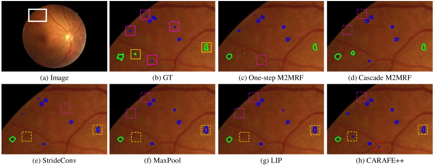
Figure 5: Visualization results on DDR test set (Li et al. 2019) by variants of HRNetV2 with different downsampling operators, i.e., our one-step M2MRF, cascade M2MRF, StrideConv (Wang et al. 2020), MaxPool, LIP (Gao, Wang, and Wu 2019) and CARAFE++ (Wang et al. 2021a). Regions delineated in green and blue are HEs and MAs by experts or segmentation approaches. As red lesions, MAs and tiny HEs have deceptive appearances and both exhibit as dark red dots. In GT map (b), challenge lesions are marked with solid boxes. In visualised segmentation result maps (c-h), wrong and miss identifications are marked with dotted boxes.

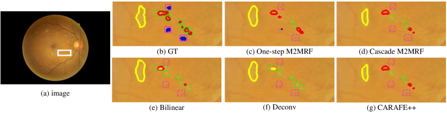
Figure 6: Visualization results on DDR test set (Li et al. 2019) by variants of HRNetV2 with different upsampling operators, i.e., our one-step M2MRF, cascade M2MRF, bilinear interpolation (Wang et al. 2020), deconvolution and CARAFE++ (Wang et al. 2021a). Regions delineated in blue, red and yellow are MAs, EXs and SEs by experts or segmentation approaches. In GT map (b), challenge lesions are marked with solid boxes. In visualised segmentation result maps (c-g), wrong and miss identifications are marked with dotted boxes.

Comparison to other RF operators

Here we verify the effectiveness of our proposed M2MRF on DDR (Li et al. 2019) testing set. In what follows, we first compare our M2MRF with downsampling and upsampling operators, and then RF operators that can/must be used as pairs.

Comparison to downsampling and upsampling operators. For downsampling, we replace strided convolution operator (StrideConv) in HRNetV2 (Wang et al. 2020) with three optional operators, i.e., strided max-pooling (MaxPool), LIP (Gao, Wang, and Wu 2019) and CARAFE++ (Wang et al. 2021a), and our two variants of M2MRF, i.e., cascade M2MRF and one-step M2MRF, and make comparisons on DDR (Li et al. 2019) test set. Among those operators, MaxPool is rule-based and parameter-free while rest are learning-based.

StrideConv is the default setting in vanilla HRNetV2 (Wang et al. 2020), whose kernel size is set to $3\times 3$ and stride is set to 2. For MaxPool, $3\times 3$ max-pooling kernel with stride of 2 is adopted. For LIP (Gao, Wang, and Wu 2019) and CARAFE++ (Wang et al. 2021a), the suggested settings by original papers are adopted. We replace StrideConv in HRNetV2 (Wang et al. 2020) with those compared downsampling operators and apply to tiny lesion segmentation. Table 2 reports their performances. We can see that: (1) Rule-based downsampling operator, i.e., MaxPool, achieves better performance than StrideConv slightly in terms of mAUPR, mF and mIoU consistently; (2) LIP (Gao, Wang, and Wu 2019) seriously degrades the segmentation performance. Possible reason is that LIP (Gao, Wang, and Wu 2019) adopts instance normalisation to normalise the importance kernels globally over entire feature map of each channel, which may heavily dilute subtle activations caused by tiny lesions and result in miss identification on tiny lesions; (3) CARAFE++ (Wang et al. 2021a) improves mAUPR by 1.06% but slightly decreases mF by 0.44% and mIoU by 0.33%; (4) Our two variants of M2MRF improve mAUPR, mF and mIoU consistently. In detail, cascade M2MRF improves mAUPR, mF and mIoU by 3.71%, 1.04% and 0.87% respectively while one-step improves mAUPR, mF and mIoU by 4.20%, 1.73% and 1.52% respectively.

We also list the parameters and inference speed of variants of HRNetV2 equipped with the compared downsampling operators in Table 2. Comparing with baseline, our proposed M2MRFs have less parameters but scarifies slight inference speed. Comparing with LIP (Gao, Wang, and Wu 2019) and CARAFE++ (Wang et al. 2021a), our proposed M2MRFs have less parameters and competitive inference speed. Obviously, HRNetV2 (Wang et al. 2020) equipped with MaxPool has least parameters and achieves fastest inference speed as MaxPool is rule-based and parameter-free.

RF operators	mAUPR	mF	mIoU	Param(M)	FPS
StrideConv/Bilinear	45.21	43.95	28.84	65.85	11.31
CARAFE++(Wang et al. 2021a)	47.64	44.80	29.54	72.57	8.69
MaxPool/Unpooling	48.81	46.17	30.73	59.45	11.62
IndexNet(Lu et al. 2020)	48.06	45.64	30.28	70.33	10.75
A2U(Dai, Lu, and Shen 2021)	45.89	44.44	29.27	66.51	3.97
M2MRF-A	49.94	46.60	31.16	69.93	9.21
M2MRF-B	49.42	45.77	30.41	67.15	8.54
M2MRF-C	48.94	45.40	30.09	70.30	8.43
M2MRF-D	49.25	45.57	30.27	67.52	8.01

Table 3: Comparing with different paired RF operators on DDR (Li et al. 2019) testing set. M2MRF-A: (one-step/one-step), M2MRF-B:(one-step/cascade), M2MRF-C:(cascade/one-step), M2MRF-D: (cascade/cascade). The first row is the baseline i.e. vanilla HRNetV2 (Wang et al. 2020). The Best and Second Best results are highlighted in boldface and underlined respectively. All results are averaged over three repetitions.

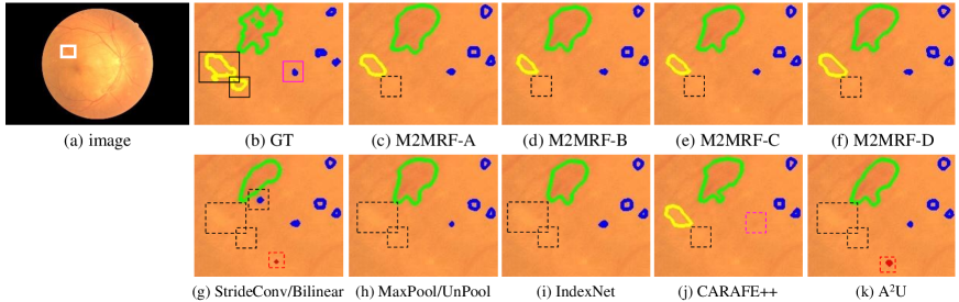
Figure 7: Visualization results on DDR test set (Li et al. 2019) by variants of HRNetV2 with paired RF operators: M2MRF-A, M2MRF-B, M2MRF-C, M2MRF-D, StrideConv/bilinear, MaxPool/UnPool, IndexNet (Lu et al. 2020), CARAFE++ (Wang et al. 2021a) and A²U (Dai, Lu, and Shen 2021). Regions delineated in green, blue, red and yellow are HEs, MAs, EXs and SEs by experts or segmentation approaches. In GT map (b), challenge lesions are marked with solid boxes. In visualised segmentation result maps (c-k), wrong and miss identifications are marked with dotted boxes.

Methods	AUPR					F					IoU
	EX	HE	SE	MA	mAUPR	EX	HE	SE	MA	mF	EX	HE	SE	MA	mIoU
HED(Xie and Tu 2015)	61.40	43.19	46.68	20.61	42.97	56.63	42.61	45.50	22.43	41.79	39.50	27.09	29.46	12.63	27.17
DNL(Yin et al. 2020)	56.05	47.81	42.01	14.71	40.14	53.36	42.71	40.40	15.60	38.02	36.39	27.15	25.33	8.46	24.33
Deeplabv3+(Chen et al. 2018)	62.32	40.79	41.83	24.39	42.34	58.59	37.97	41.83	25.40	40.95	41.44	23.44	26.46	14.55	26.47
PSPNet(Zhao et al. 2017)	57.04	42.71	42.32	14.85	39.23	54.35	39.37	42.08	16.09	37.97	37.31	24.51	26.64	8.75	24.31
SPNet(Hou et al. 2020)	44.10	38.22	32.93	12.37	31.91	38.78	24.13	34.00	13.74	27.66	24.19	13.76	20.55	7.38	16.47
L-seg (Guo et al. 2019)	55.46	35.86	26.48	10.52	32.08	-	-	-	-	-	-	-	-	-	-
HRNetV2(Wang et al. 2020)	61.55	45.68	46.91	26.70	45.21	58.98	44.96	44.86	26.99	43.95	41.82	29.01	28.94	15.60	28.84
Swin-base(Liu et al. 2021b)	62.95	53.46	50.56	23.46	47.61	60.12	51.10	50.85	23.38	46.36	42.98	34.42	34.15	13.24	31.20
Twins-SVT-B (Chu et al. 2021)	59.71	49.96	52.72	22.03	46.11	56.83	45.04	53.19	21.54	44.15	39.70	29.08	36.24	12.07	29.28
M2MRF-A	64.17	54.20	53.19	28.21	49.94	60.47	46.18	52.10	27.67	46.60	43.35	30.03	35.22	16.06	31.16
M2MRF-B	63.88	55.47	50.01	28.33	49.42	60.20	46.81	48.58	27.51	45.77	43.06	30.56	32.08	15.95	30.41
M2MRF-C	63.59	54.43	49.35	28.38	48.94	60.62	45.16	47.78	28.04	45.40	43.49	29.17	31.39	16.31	30.09
M2MRF-D	64.17	54.72	49.64	28.46	49.25	61.15	45.29	48.02	27.81	45.57	44.04	29.28	31.60	16.15	30.27

Table 4: Segmentation results on DDR test set (Li et al. 2019). M2MRF-A: (one-step/one-step), M2MRF-B:(one-step/cascade), M2MRF-C:(cascade/one-step), M2MRF-D: (cascade/cascade). The Best and Second Best results are highlighted in boldface and underlined respectively. All results are averaged over three repetitions.

To further illustrate the superiority of our M2MRFs as downsampling operators, we visualise segmentation results on MAs and HEs in Fig. 5. The reason of choosing these two types of lesions is that MAs and tiny HEs belong to red lesions and exhibit as dark red dots with similar appearances. Correctly identifying them requires that segmentation models are able to maintain subtle activations about them and exploit long-range dependencies to boost the discriminativeness of activations during downsampling. For clarity, we mark challenge MAs with solid magenta boxes and HEs with solid yellow boxes in GT map (see Fig. 5(b)) and miss and wrong identifications by variants of HRNetv2 (Wang et al. 2020) utilising different downsampling operators in Fig. 5 (c-h) with dotted boxes. Obviously, our proposed cascade M2MRF and one-step M2MRF (see Fig. 5(c-d)) encounter less miss and wrong identifications than compared four downsampling operators as shown in Fig. 5(e-h). Particularly, both of our cascade M2MRF and one-step M2MRF are able to correctly distinguish between HEs and MAs while variants of HRNetv2 (Wang et al. 2020) with rest downsampling operators are prone to be deceived by their confusion appearances and wrongly identify HEs as MAs. Although CARAFE++ (Wang et al. 2021a) is able to maintain subtle activations about tiny lesions, it seems scarifies the feature discrimination and tends to cause wrong identifications.

For upsampling, we utilise strided convolution for downsampling and replace bilinear interpolation in HRNetV2 (Wang et al. 2020) with four optional upsampling operators, i.e., deconvolution and CARAFE++ (Wang et al. 2021a), our proposed cascade M2MRF and one-step M2MRF. Among them, bilinear interpolation is rule-based and parameter-free while the rest are learning-based. We compare their performance on DDR (Li et al. 2019) test set. As reported in Table 2, comparing with bilinear interpolation, our two variants of M2MRF achieve slightly better mAUPR, mF and mIoU but require extra parameters and inference time. From Table 2 we also can see that, different to CARAFE++ (Wang et al. 2021a) which works better as upsampling operator than downsample operator, our M2MRFs work better as downsampling operators. Fig. 6 shows visualised segmentation results. As exampled, it is challenge to well segment tiny lesions clustering together. Comparatively speaking, our one-step M2MRF, cascade M2MRF and CARAFE++ (Wang et al. 2021a) make less mistakes than bilinear interpolation and deconvolution.

Comparison to paired RF operators. We have four different RF pairs when combining cascade M2MRF and one-step M2MRF for both downsampling and upsampling. We denote them by M2MRF-A (one-step M2MRF for both downsampling and upsampling), M2MRF-B (one-step M2MRF for downsampling and cascade M2MRF for upsampling), M2MRF-C (cascade M2MRF for downsampling and one-step M2MRF for upsampling), M2MRF-D (cascade M2MRF for both downsampling and upsampling). We compare them with five pairs of RF operators, i.e., StrideConv/Bilinear, CARAFE++ (Wang et al. 2021a), MaxPool/Unpooling, IndexNet (Lu et al. 2020) and A²U (Dai, Lu, and Shen 2021) on DDR (Li et al. 2019) test set. Among those RF operators, MaxPool/Unpooling and IndexNet (Lu et al. 2020) have to utilise the indices generated during downsampling for upsampling. Table 3 reports quantitative results. As listed, among four variants of our M2MRF, M2MRF-A achieves best in mAUPR, mF and mIoU. Comparing with vanilla HRNetV2 (Wang et al. 2020), our M2MRF-A improves the mAUPR by a large margin from 45.21% to 49.94% and the mIoU from 28.84% to 31.16% with few extra parameters (65.85M$\rightarrow$69.93M) and slightly slower inference speed (11.31fps$\rightarrow$9.21fps). Comparing with existing RF operators, our M2MRF-A achieves best in both mAUPR and mIoU and the rest three variants achieve better mAUPR and competitive mIoU. Specifically, comparing with the recent learning-based RF operators IndexNet (Lu et al. 2020) and CARAFE++ (Wang et al. 2021a), our M2MRF-A and M2MRF-B achieve better performance in mAUPR and mIoU with less parameters and competitive inference speed. Comparing with A²U (Dai, Lu, and Shen 2021), our four variants of M2MRF outperform it on both mAPUR and mIoU with faster inference speed. Fig. 7 shows visualised segmentation results, from which we can see that our four variants of M2MRF are able to preserve very subtle lesion activations and make less mistakes than those compared paired RFs.

Comparison to state-of-the-art segmentation methods

We compare our M2MRF-HRNetV2 with nine state-of-the-art segmentation approaches as listed in Table 4. The first seven methods are CNN-based and the rest two are transformer-based. Results by Swin-base (Liu et al. 2021b) are obtained by fine-tuning the pre-trained model on ImageNet-22K with DDR training set (Li et al. 2019) and the rest are obtained by fine-tuning the pre-trained models on ImageNet-1K (Krizhevsky, Sutskever, and Hinton 2012). As we can see that: (1) among previous CNN-based segmentation methods, the vanilla HRNetV2 (Wang et al. 2020) achieves best performance with 45.21% on mAUPR, 43.95% on mF and 28.84% on mIoU; (2) comparing with vanilla HRNetV2 (Wang et al. 2020), the four variants of our M2MRF get better performance on the four lesion classes consistently in terms of mAUPR, mF and mIoU; (3) comparing with one of the most recent transformer-based methods, Swin-base (Liu et al. 2021b), our four variants of M2MRF achieve better on mAUPR by a large margin while our M2MRF-A achieves competitive performance on mF and mIoU; (4) comparing with another transform-based method Twins-SVT-B (Chu et al. 2021), the four variants of our M2MRF surpass it significantly and consistently on mAUPR, mF and mIoU.

RF operators	mAUPR	mF	mIoU
StrideConv/Bilinear	65.01	63.14	47.52
MaxPool/Bilinear	66.24	65.01	49.28
LIP (Gao, Wang, and Wu 2019)/Bilinear	63.04	61.50	45.78
StrideConv/Deconv	64.64	62.86	47.23
MaxPool/Unpooling	66.17	64.98	49.22
CARAFE++ (Wang et al. 2021a)	66.35	64.67	48.91
IndexNet (Lu et al. 2020)	65.77	64.30	48.74
A2U (Dai, Lu, and Shen 2021)	64.93	63.23	47.52
M2MRF-A	66.48	64.89	49.07
M2MRF-B	66.00	64.45	48.56
M2MRF-C	67.24	65.71	49.94
M2MRF-D	66.66	65.15	49.36

Table 5: Comparing with different RF operators on IDRiD (Porwal et al. 2020) testing set. The first row is the baseline i.e. vanilla HRNetV2 (Wang et al. 2020). A: (one-step/one-step), B:(one-step/cascade), C:(cascade/one-step), D: (cascade/cascade). All results are averaged over three repetitions.

Methods	AUPR					F					IoU
	EX	HE	SE	MA	mAUPR	EX	HE	SE	MA	mF	EX	HE	SE	MA	mIoU
VRT(1st)(Porwal et al. 2020)	71.27	68.04	69.95	49.51	64.69	-	-	-	-	-	-	-	-	-	-
PATech(2nd)(Porwal et al. 2020)	88.50	64.90	-	47.70	-	-	-	-	-	-	-	-	-	-	-
iFLYTEK(3rd)(Porwal et al. 2020)	87.41	55.88	65.88	50.17	64.84	-	-	-	-	-	-	-	-	-	-
L-seg(Guo et al. 2019)	79.45	63.74	71.13	46.27	65.15	-	-	-	-	-	-	-	-	-	-
HED(Xie and Tu 2015)	80.81	66.41	68.09	40.45	63.94	78.60	64.33	67.00	38.81	62.18	64.74	47.43	50.38	24.07	46.66
DNL(Yin et al. 2020)	75.12	64.04	64.73	32.48	59.09	73.15	61.87	63.96	32.78	57.94	57.67	44.80	47.03	19.61	42.28
Deeplabv3+(Chen et al. 2018)	81.93	64.66	63.04	43.14	63.19	79.60	61.96	61.48	40.57	60.90	66.10	44.90	44.39	25.45	45.21
PSPNet(Zhao et al. 2017)	75.21	63.36	63.65	32.71	58.73	73.24	60.81	62.83	32.63	57.38	57.78	43.71	45.81	19.50	41.70
SPNet(Hou et al. 2020)	64.61	54.11	52.14	30.14	50.25	61.45	44.33	49.59	25.66	45.26	44.40	28.50	33.58	14.72	30.30
HRNetV2(Wang et al. 2020)	82.09	65.50	68.68	43.76	65.01	79.93	62.58	67.53	42.49	63.14	66.57	45.56	50.99	26.98	47.52
Swin-base(Liu et al. 2021b)	81.30	67.70	66.46	44.19	64.91	79.64	66.42	66.00	44.09	64.04	66.17	49.72	49.27	28.28	48.36
Twins-SVT-B (Chu et al. 2021)	80.09	63.12	68.86	43.27	63.84	78.56	61.98	68.19	42.42	62.79	64.68	44.91	51.76	26.92	47.07
M2MRF-A	82.04	67.80	68.23	47.86	66.48	79.64	65.66	66.68	47.59	64.89	66.16	48.87	50.03	31.23	49.07
M2MRF-B	81.98	67.41	66.68	47.91	66.00	79.57	65.39	65.01	47.81	64.45	66.07	48.58	48.16	31.42	48.56
M2MRF-C	82.16	68.69	69.32	48.80	67.24	79.85	66.42	67.92	48.63	65.71	66.46	49.72	51.43	32.13	49.94
M2MRF-D	82.29	66.94	69.00	48.43	66.66	79.97	64.88	67.50	48.26	65.15	66.62	48.04	50.98	31.81	49.36

Table 6: Results on IDRiD (Porwal et al. 2020). M2MRF-A: (one-step/one-step), M2MRF-B:(one-step/cascade), M2MRF-C:(cascade/one-step), M2MRF-D: (cascade/cascade). The Best and Second Best results are highlighted in boldface and underlined respectively.

Results on IDRiD

Comparison to state-of-the-art RF operators

To further validate the effectiveness of our proposed M2MRF, we conduct experiments on IDRiD (Porwal et al. 2020) and make comparisons with existing eight pairs of RF operators. Table 5 reports the results. It shows that M2MRF-C, i.e., cascade M2MRF for downsampling and one-step M2MRF for upsampling ranks first while our M2MRF-D, i.e., cascade M2MRF for both downsampling and upsampling ranks second among listed competitors. Particularly, our M2MRF-C surpasses the baseline consistently in terms of mAUPR (67.24% vs. 65.01%), mF (65.71% vs. 63.14%) and mIoU (49.94% vs. 47.52%) by a large margin. Interestingly, two pairs of rule-based RF operators, i.e., MaxPool/Bilinear interpolation and MaxPool/Unpooling achieve better than previous learning-based RF operators. The possible reason is that it may be difficult for learning-based RF operators to preserve activations caused by tiny lesions via learning from a small local region with limited size of receptive field.

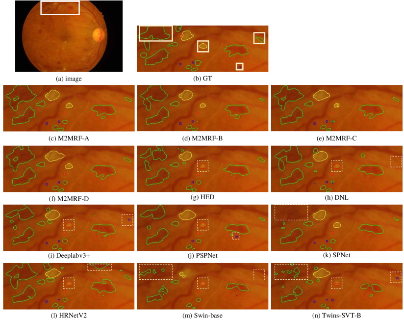
Figure 8: Segmentation results on IDRiD test set (Porwal et al. 2020). From (a) to (n) are original image, patch with lesion annotations by experts, results by our M2MRF-A/B/C/D, HED (Xie and Tu 2015), DNL (Yin et al. 2020), Deeplabv3+ (Chen et al. 2018), PSPNet (Zhao et al. 2017), SPNet (Hou et al. 2020), HRNetV2 (Wang et al. 2020), Swin-base (Liu et al. 2021b) and Twins-SVT-B (Chu et al. 2021). Regions delineated in green, blue and red are HEs, MAs and EXs by experts or segmentation approaches. Lesions marked with solid golden boxes in (b) are challenge lesions. Four variants of HRNetV2 (Wang et al. 2020) equipped with our M2MRFs are almost able to correctly segment those challenge lesions while compared methods are prone to encounter either miss or wrong identifications which are marked with dotted golden boxes.

Comparison to state-of-the-art segmentation methods

We compare our M2MRF with four tiny lesion segmentation methods (VRT, PATech, iFLYTEK (Porwal et al. 2020) and L-seg (Guo et al. 2019)), six state-of-the-art CNN-based methods and two recent transformer-based methods (Swin-base (Liu et al. 2021b) and Twins-SVT-B (Chu et al. 2021)). Among four tiny lesion segmentation methods, performance of L-Seg (Guo et al. 2019) is directly borrowed from original paper and the rest are top three methods borrowed from the 2018 ISBI grand challenge. Results of six CNN-based segmentation methods and Twins-SVT-B (Chu et al. 2021) are obtained via fine-tuning pre-trained model on ImageNet1K (Krizhevsky, Sutskever, and Hinton 2012) with IDRiD (Porwal et al. 2020) training set while Swin-base (Liu et al. 2021b) is ImageNet-22K.

Table 6 reports comparison results, from which we have following observations: (1) Our four variants of M2MRF surpass all the competitors consistently in terms of mAUPR, mF and mIoU; (2) They contribute significantly to MA segmentation and outperform vanilla HRNetV2 (Wang et al. 2020) by more than 4% on AUPR, 5% on F-score and 4% on IoU, which indicates that our M2MRF is able to maintain more subtle activations about tiny lesions; (3) Among them, our M2MRF-C achieves best performance, which surpasses the most recent transformer-based segmentation method Swin-base (Liu et al. 2021b) by 2.33%, 1.67% and 1.58% in mAUPR, mF and mIoU respectively; (4) Methods specially designed for lesion segmentation achieve better in mAUPR than the compared CNN-based methods except for HRNetV2 (Wang et al. 2020); (5) HRNetV2 (Wang et al. 2020) is a strong baseline on tiny lesion segmentation task and achieves competitive mAUPR to methods participating grand challenge as it learns high-resolution representations with detailed spatial information. We also make qualitative comparison to compared state-of-the-art methods and visualise their results in Fig. 8.

Conclusion

We present a simple RF operator named M2MRF for feature reassembly which unifies feature downsampling and upsampling in one framework. Our M2MRF considers contributions of long range spatial dependencies and simultaneously reassembles multiple features in a large region to multiple target features once. Thus, it is able to maintain activations caused by tiny lesions during feature reassembly. It shows significant improvements on two public tiny lesion segmentation datasets, i.e. DDR (Li et al. 2019) and IDRiD (Porwal et al. 2020). Moreover, our M2MRF only introduces marginal extra parameters and could be used to replace arbitrary RF operators in existing CNN architectures.

References

- Badrinarayanan, Kendall, and Cipolla (2017) Badrinarayanan, V.; Kendall, A.; and Cipolla, R. 2017. Segnet: A deep convolutional encoder-decoder architecture for image segmentation. TPAMI, 39(12): 2481–2495.
- Chen et al. (2017) Chen, L.-C.; Papandreou, G.; Kokkinos, I.; Murphy, K.; and Yuille, A. L. 2017. Deeplab: Semantic image segmentation with deep convolutional nets, atrous convolution, and fully connected crfs. TPAMI, 40(4): 834–848.
- Chen et al. (2018) Chen, L.-C.; Zhu, Y.; Papandreou, G.; Schroff, F.; and Adam, H. 2018. Encoder-decoder with atrous separable convolution for semantic image segmentation. In ECCV, 801–818.
- Chen et al. (2020) Chen, W.; Zhu, X.; Sun, R.; He, J.; Li, R.; Shen, X.; and Yu, B. 2020. Tensor Low-Rank Reconstruction for Semantic Segmentation. In ECCV, 52–69. Springer.
- Choi, Kim, and Choo (2020) Choi, S.; Kim, J. T.; and Choo, J. 2020. Cars Can’t Fly Up in the Sky: Improving Urban-Scene Segmentation via Height-Driven Attention Networks. In CVPR, 9373–9383.
- Chu et al. (2021) Chu, X.; Tian, Z.; Wang, Y.; Zhang, B.; Ren, H.; Wei, X.; Xia, H.; and Shen, C. 2021. Twins: Revisiting the Design of Spatial Attention in Vision Transformers. In NeurIPS.
- Contributors (2020) Contributors, M. 2020. MMSegmentation: OpenMMLab Semantic Segmentation Toolbox and Benchmark. https://github.com/open-mmlab/mmsegmentation.
- Cordts et al. (2016) Cordts, M.; Omran, M.; Ramos, S.; Rehfeld, T.; Enzweiler, M.; Benenson, R.; Franke, U.; Roth, S.; and Schiele, B. 2016. The cityscapes dataset for semantic urban scene understanding. In CVPR, 3213–3223.
- Dai et al. (2017) Dai, J.; Qi, H.; Xiong, Y.; Li, Y.; Zhang, G.; Hu, H.; and Wei, Y. 2017. Deformable convolutional networks. In ICCV, 764–773.
- Dai, Lu, and Shen (2021) Dai, Y.; Lu, H.; and Shen, C. 2021. Learning Affinity-Aware Upsampling for Deep Image Matting. In CVPR, 6841–6850.
- Decenciere et al. (2013) Decenciere, E.; Cazuguel, G.; Zhang, X.; Thibault, G.; Klein, J.-C.; Meyer, F.; Marcotegui, B.; Quellec, G.; Lamard, M.; Danno, R.; et al. 2013. TeleOphta: Machine learning and image processing methods for teleophthalmology. Irbm, 34(2): 196–203.
- Dong et al. (2021) Dong, X.; Bao, J.; Chen, D.; Zhang, W.; Yu, N.; Yuan, L.; Chen, D.; and Guo, B. 2021. CSWin Transformer: A General Vision Transformer Backbone with Cross-Shaped Windows. arXiv:2107.00652.
- Du et al. (2020) Du, J.; Zou, B.; Chen, C.; Xu, Z.; and Liu, Q. 2020. Automatic microaneurysm detection in fundus image based on local cross-section transformation and multi-feature fusion. Computer Methods and Programs in Biomedicine, 196: 105687.
- Foo et al. (2020) Foo, A.; Hsu, W.; Lee, M. L.; Lim, G.; and Wong, T. Y. 2020. Multi-task learning for diabetic retinopathy grading and lesion segmentation. In AAAI, volume 34, 13267–13272.
- Fu et al. (2018) Fu, H.; Cheng, J.; Xu, Y.; Wong, D. W. K.; Liu, J.; and Cao, X. 2018. Joint optic disc and cup segmentation based on multi-label deep network and polar transformation. TMI, 37(7): 1597–1605.
- Fu et al. (2020) Fu, J.; Liu, J.; Jiang, J.; Li, Y.; Bao, Y.; and Lu, H. 2020. Scene segmentation with dual relation-aware attention network. TNNLS.
- Fu et al. (2019) Fu, J.; Liu, J.; Tian, H.; Li, Y.; Bao, Y.; Fang, Z.; and Lu, H. 2019. Dual attention network for scene segmentation. In CVPR, 3146–3154.
- Gao, Wang, and Wu (2019) Gao, Z.; Wang, L.; and Wu, G. 2019. Lip: Local importance-based pooling. In ICCV, 3355–3364.
- Guo et al. (2019) Guo, S.; Li, T.; Kang, H.; Li, N.; Zhang, Y.; and Wang, K. 2019. L-Seg: An end-to-end unified framework for multi-lesion segmentation of fundus images. Neurocomputing, 349: 52–63.
- Hou et al. (2020) Hou, Q.; Zhang, L.; Cheng, M.-M.; and Feng, J. 2020. Strip pooling: Rethinking spatial pooling for scene parsing. In CVPR, 4003–4012.
- Huang et al. (2019) Huang, Z.; Wang, X.; Huang, L.; Huang, C.; Wei, Y.; and Liu, W. 2019. Ccnet: Criss-cross attention for semantic segmentation. In ICCV, 603–612.
- Krizhevsky, Sutskever, and Hinton (2012) Krizhevsky, A.; Sutskever, I.; and Hinton, G. E. 2012. Imagenet classification with deep convolutional neural networks. In NIPS, 84–90. AcM New York, NY, USA.
- LeCun et al. (1990) LeCun, Y.; Boser, B. E.; Denker, J. S.; Henderson, D.; Howard, R. E.; Hubbard, W. E.; and Jackel, L. D. 1990. Handwritten digit recognition with a back-propagation network. In NeurIPS, 396–404.
- Li et al. (2019) Li, T.; Gao, Y.; Wang, K.; Guo, S.; Liu, H.; and Kang, H. 2019. Diagnostic assessment of deep learning algorithms for diabetic retinopathy screening. Information Sciences, 501: 511–522.
- Li et al. (2020) Li, X.; Zhao, H.; Han, L.; Tong, Y.; Tan, S.; and Yang, K. 2020. Gated Fully Fusion for Semantic Segmentation. In AAAI, volume 34, 11418–11425.
- Liu et al. (2019) Liu, Q.; Hong, X.; Li, S.; Chen, Z.; Zhao, G.; and Zou, B. 2019. A spatial-aware joint optic disc and cup segmentation method. Neurocomputing, 359: 285–297.
- Liu et al. (2021a) Liu, Q.; Liu, H.; Zhao, Y.; and Liang, Y. 2021a. Dual-Branch Network with Dual-Sampling Modulated Dice Loss for Hard Exudate Segmentation in Colour Fundus Images. IEEE J-BHI, 1–1.
- Liu et al. (2017) Liu, Q.; Zou, B.; Chen, J.; Ke, W.; Yue, K.; Chen, Z.; and Zhao, G. 2017. A location-to-segmentation strategy for automatic exudate segmentation in colour retinal fundus images. Computerized medical imaging and graphics, 55: 78–86.
- Liu et al. (2021b) Liu, Z.; Lin, Y.; Cao, Y.; Hu, H.; Wei, Y.; Zhang, Z.; Lin, S.; and Guo, B. 2021b. Swin transformer: Hierarchical vision transformer using shifted windows. In ICCV.
- Long, Shelhamer, and Darrell (2015) Long, J.; Shelhamer, E.; and Darrell, T. 2015. Fully convolutional networks for semantic segmentation. In CVPR, 3431–3440.
- Lu et al. (2019) Lu, H.; Dai, Y.; Shen, C.; and Xu, S. 2019. Indices matter: Learning to index for deep image matting. In ICCV, 3266–3275.
- Lu et al. (2020) Lu, H.; Dai, Y.; Shen, C.; and Xu, S. 2020. Index networks. TPAMI.
- Milletari, Navab, and Ahmadi (2016) Milletari, F.; Navab, N.; and Ahmadi, S. 2016. V-Net: Fully Convolutional Neural Networks for Volumetric Medical Image Segmentation. In 2016 Fourth International Conference on 3D Vision (3DV), 565–571.
- Noh, Hong, and Han (2015) Noh, H.; Hong, S.; and Han, B. 2015. Learning deconvolution network for semantic segmentation. In ICCV, 1520–1528.
- Porwal et al. (2020) Porwal, P.; Pachade, S.; Kokare, M.; Deshmukh, G.; Son, J.; Bae, W.; Liu, L.; Wang, J.; Liu, X.; Gao, L.; et al. 2020. IDRiD: Diabetic Retinopathy–Segmentation and Grading Challenge. Medical Image Analysis, 59: 101561.
- Ronneberger, Fischer, and Brox (2015) Ronneberger, O.; Fischer, P.; and Brox, T. 2015. U-net: Convolutional networks for biomedical image segmentation. In MICCAI, 234–241. Springer.
- Springenberg et al. (2015) Springenberg, J. T.; Dosovitskiy, A.; Brox, T.; and Riedmiller, M. 2015. Striving for simplicity: The all convolutional net. In ICLR workshop.
- Sun et al. (2019) Sun, K.; Xiao, B.; Liu, D.; and Wang, J. 2019. Deep high-resolution representation learning for human pose estimation. In CVPR, 5693–5703.
- Sun et al. (2021) Sun, R.; Li, Y.; Zhang, T.; Mao, Z.; Wu, F.; and Zhang, Y. 2021. Lesion-Aware Transformers for Diabetic Retinopathy Grading. In CVPR, 10938–10947.
- Wang et al. (2019) Wang, J.; Chen, K.; Xu, R.; Liu, Z.; Loy, C. C.; and Lin, D. 2019. Carafe: Content-aware reassembly of features. In ICCV, 3007–3016.
- Wang et al. (2021a) Wang, J.; Chen, K.; Xu, R.; Liu, Z.; Loy, C. C.; and Lin, D. 2021a. CARAFE++: Unified Content-Aware ReAssembly of FEatures. TPAMI.
- Wang et al. (2020) Wang, J.; Sun, K.; Cheng, T.; Jiang, B.; Deng, C.; Zhao, Y.; Liu, D.; Mu, Y.; Tan, M.; Wang, X.; et al. 2020. Deep high-resolution representation learning for visual recognition. TPAMI.
- Wang et al. (2021b) Wang, X.; Xu, M.; Zhang, J.; Jiang, L.; and Li, L. 2021b. Deep Multi-Task Learning for Diabetic Retinopathy Grading in Fundus Images. In AAAI, volume 35, 2826–2834.
- Xie and Tu (2015) Xie, S.; and Tu, Z. 2015. Holistically-nested edge detection. In ICCV, 1395–1403.
- Yin et al. (2020) Yin, M.; Yao, Z.; Cao, Y.; Li, X.; Zhang, Z.; Lin, S.; and Hu, H. 2020. Disentangled non-local neural networks. In ECCV, 191–207. Springer.
- Zeiler and Fergus (2014) Zeiler, M. D.; and Fergus, R. 2014. Visualizing and understanding convolutional networks. In ECCV, 818–833. Springer.
- Zeiler et al. (2010) Zeiler, M. D.; Krishnan, D.; Taylor, G. W.; and Fergus, R. 2010. Deconvolutional networks. In CVPR, 2528–2535. IEEE.
- Zeiler, Taylor, and Fergus (2011) Zeiler, M. D.; Taylor, G. W.; and Fergus, R. 2011. Adaptive deconvolutional networks for mid and high level feature learning. In ICCV, 2018–2025. IEEE.
- Zhang et al. (2014) Zhang, X.; Thibault, G.; Decencière, E.; Marcotegui, B.; Laÿ, B.; Danno, R.; Cazuguel, G.; Quellec, G.; Lamard, M.; Massin, P.; et al. 2014. Exudate detection in color retinal images for mass screening of diabetic retinopathy. Medical image analysis, 18(7): 1026–1043.
- Zhao et al. (2017) Zhao, H.; Shi, J.; Qi, X.; Wang, X.; and Jia, J. 2017. Pyramid scene parsing network. In CVPR, 2881–2890.
- Zhou et al. (2019) Zhou, Z.; Siddiquee, M. M. R.; Tajbakhsh, N.; and Liang, J. 2019. Unet++: Redesigning skip connections to exploit multiscale features in image segmentation. TMI, 39(6): 1856–1867.