Generalized Data Weighting via Class-level Gradient Manipulation

Abstract

Label noise and class imbalance are two major issues coexisting in real-world datasets. To alleviate the two issues, state-of-the-art methods reweight each instance by leveraging a small amount of clean and unbiased data. Yet, these methods overlook class-level information within each instance, which can be further utilized to improve performance. To this end, in this paper, we propose Generalized Data Weighting (GDW) to simultaneously mitigate label noise and class imbalance by manipulating gradients at the class level. To be specific, GDW unrolls the loss gradient to class-level gradients by the chain rule and reweights the flow of each gradient separately. In this way, GDW achieves remarkable performance improvement on both issues. Aside from the performance gain, GDW efficiently obtains class-level weights without introducing any extra computational cost compared with instance weighting methods. Specifically, GDW performs a gradient descent step on class-level weights, which only relies on intermediate gradients. Extensive experiments in various settings verify the effectiveness of GDW. For example, GDW outperforms state-of-the-art methods by $2.56\%$ under the $60\%$ uniform noise setting in CIFAR10. Our code is available at https://github.com/GGchen1997/GDW-NIPS2021.

1 Introduction

Real-world classification datasets often suffer from two issues, i.e., label noise songLearningNoisyLabels2021 and class imbalance heLearningImbalancedData2009 . On the one hand, label noise often results from the limitation of data generation, e.g., sensor errors elhadySystematicSurveySensor2018a and mislabeling from crowdsourcing workers tongxiaoLearningMassiveNoisy2015 . Label noise misleads the training process of DNNs and degrades the model performance in various aspects alganLabelNoiseTypes2020b ; zhuClassNoiseVs2004a ; frenayClassificationPresenceLabel2014a . On the other hand, imbalanced datasets are either naturally long-tailed zhaoLongTailDistributionsUnsupervised2012a ; vanhornDevilTailsFinegrained2017a or biased from the real-world distribution due to imperfect data collection pavonAssessingImpactClassImbalanced2011a ; patelReviewClassificationImbalanced2020a . Training with imbalanced datasets usually results in poor classification performance on weakly represented classes dongClassRectificationHard2017a ; cuiClassBalancedLossBased2019 ; sinhaClassWiseDifficultyBalancedLoss2021a . Even worse, these two issues often coexist in real-world datasets johnsonSurveyDeepLearning2019a .

To prevent the model from memorizing noisy information, many important works have been proposed, including label smoothing szegedyRethinkingInceptionArchitecture2016a , noise adaptation goldbergerTrainingDeepNeuralnetworks2017 , importance weighting liuClassificationNoisyLabels2014 , GLC hendrycksUsingTrustedData2018 , and Co-teach hanCoteachingRobustTraining2018a . Meanwhile, dongClassRectificationHard2017a ; cuiClassBalancedLossBased2019 ; sinhaClassWiseDifficultyBalancedLoss2021a ; linFocalLossDense2020 propose effective methods to tackle class imbalance. However, these methods inevitably introduce hyper-parameters (e.g., the weighting factor in cuiClassBalancedLossBased2019 and the focusing parameter in linFocalLossDense2020 ), compounding real-world deployment.

Inspired by recent advances in meta-learning, some works renLearningReweightExamples2018 ; shuMetaWeightNetLearningExplicit2019a ; huLearningDataManipulation2019a ; wangOptimizingDataUsage2020b propose to solve both issues by leveraging a clean and unbiased meta set. These methods treat instance weights as hyper-parameters and dynamically update these weights to circumvent hyper-parameter tuning. Specifically, MWNet shuMetaWeightNetLearningExplicit2019a adopts an MLP with the instance loss as input and the instance weight as output. Due to the MLP, MWNet has better scalability on large datasets compared with INSW huLearningDataManipulation2019a which assigns each instance with a learnable weight. Although these methods can handle label noise and class imbalance to some extent, they cannot fully utilize class-level information within each instance, resulting in the potential loss of useful information. For example, in a three-class classification task, every instance has three logits. As shown in Figure 1, every logit corresponds to a class-level gradient flow which stems from the loss function and back-propagates. These gradient flows represent three kinds of information: "not cat", "dog", and "not bird". Instance weighting methods shuMetaWeightNetLearningExplicit2019a ; renLearningReweightExamples2018 alleviate label noise by downweighting all the gradient flows of the instance, which discards three kinds of information simultaneously. Yet, downweighting the "not bird" gradient flow is a waste of information. Similarly, in class imbalance scenarios, different gradient flows represent different class-level information.

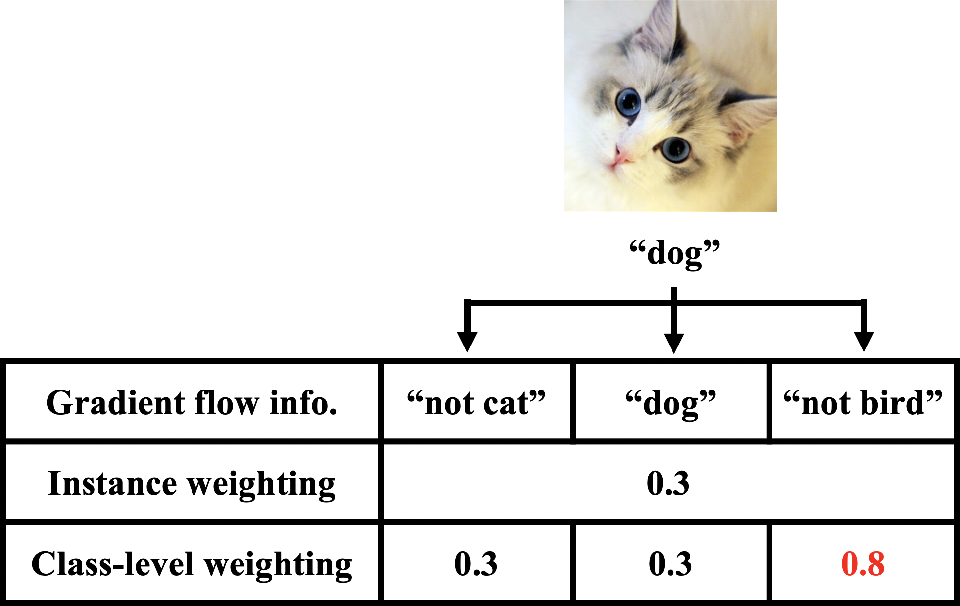
Figure 1: Motivation for class-level weighting. For a noisy instance (e.g. cat mislabeled as "dog"), all gradient flows are downweighted by instance weighting. Although the gradient flows for "dog" and "not cat" contain harmful information, the gradient flow for "not bird" is still valuable for training, which should not be downweighted.

Therefore, it is necessary to reweight instances at the class level for better information usage.

To this end, we propose Generalized Data Weighting (GDW) to tackle label noise and class imbalance by class-level gradient manipulation. Firstly, we introduce class-level weights to represent the importance of different gradient flows and manipulate the gradient flows with these class-level weights. Secondly, we impose a zero-mean constraint on class-level weights for stable training. Thirdly, to efficiently obtain class-level weights, we develop a two-stage weight generation scheme embedded in bi-level optimization. As a side note, the instance weighting methods renLearningReweightExamples2018 ; shuMetaWeightNetLearningExplicit2019a ; huLearningDataManipulation2019a ; wangOptimizingDataUsage2020b can be considered special cases of GDW when class-level weights within any instance are the same. In this way, GDW achieves impressive performance improvement in various settings.

To sum up, our contribution is two-fold:

1. For better information utilization, we propose GDW, a generalized data weighting method, which better handles label noise and class imbalance. To the best of our knowledge, we are the first to propose single-label class-level weighting on gradient flows.

2. To obtain class-level weights efficiently, we design a two-stage scheme embedded in a bi-level optimization framework, which does not introduce any extra computational cost. To be specific, during the back-propagation we store intermediate gradients, with which we update class-level weights via a gradient descent step.

2 Related Works

2.1 Non-Meta-Learning Methods for Label Noise

Label noise is a common problem in classification tasks zhuClassNoiseVs2004a ; frenayClassificationPresenceLabel2014a ; alganLabelNoiseTypes2020b . To avoid overfitting to label noise, szegedyRethinkingInceptionArchitecture2016a propose label smoothing to regularize the model. goldbergerTrainingDeepNeuralnetworks2017 ; vahdatRobustnessLabelNoise2017a form different models to indicate the relation between noisy instances and clean instances. liuClassificationNoisyLabels2014 estimate an importance weight for each instance to represent its value to the model. hanCoteachingRobustTraining2018a train two models simultaneously and let them teach each other in every mini-batch. However, without a clean dataset, these methods cannot handle severe noise renLearningReweightExamples2018 . hendrycksUsingTrustedData2018 correct the prediction of the model by estimating the label corruption matrix via a clean validation set, but this matrix is the same across all instances. Instead, our method generates dynamic class-level weights for every instance to improve training.

2.2 Non-Meta-Learning Methods for Class Imbalance

Many important works have been proposed to handle class imbalance elkanFoundationsCostsensitiveLearning2001 ; chawlaSMOTESyntheticMinority2002a ; anandApproachClassificationHighly2010a ; dongClassRectificationHard2017a ; khanCostSensitiveLearningDeep2018 ; cuiClassBalancedLossBased2019 ; kangDecouplingRepresentationClassifier2019 ; linFocalLossDense2020 ; sinhaClassWiseDifficultyBalancedLoss2021a . chawlaSMOTESyntheticMinority2002a ; anandApproachClassificationHighly2010a propose to over-sample the minority class and under-sample the majority class. elkanFoundationsCostsensitiveLearning2001 ; khanCostSensitiveLearningDeep2018 learn a class-dependent cost matrix to obtain robust representations for both majority and minority classes. dongClassRectificationHard2017a ; cuiClassBalancedLossBased2019 ; linFocalLossDense2020 ; sinhaClassWiseDifficultyBalancedLoss2021a design a reweighting scheme to rebalance the loss for each class. These methods are quite effective, whereas they need to manually choose loss functions or hyper-parameters. liuLargeScaleLongTailedRecognition2019 ; wangLongtailedRecognitionRouting2020 manipulate the feature space to handle class imbalance while introducing extra model parameters. kangDecouplingRepresentationClassifier2019 decouple representation learning and classifier learning on long-tailed datasets, but with extra hyper-parameter tuning. In contrast, meta-learning methods view instance weights as hyper-parameters and dynamically update them via a meta set to avoid hyper-parameter tuning.

2.3 Meta-Learning Methods

With recent development in meta-learning lakeHumanlevelConceptLearning2015a ; franceschiBilevelProgrammingHyperparameter2018a ; liuDARTSDifferentiableArchitecture2018 , many important methods have been proposed to handle label noise and class imbalance via a meta set wangLearningModelTail2017 ; jiangMentorNetLearningDataDriven2018a ; renLearningReweightExamples2018 ; liLearningLearnNoisy2019a ; shuMetaWeightNetLearningExplicit2019a ; huLearningDataManipulation2019a ; wangOptimizingDataUsage2020b ; alganMetaSoftLabel2021a . jiangMentorNetLearningDataDriven2018a propose MentorNet to provide a data-driven curriculum for the base network to focus on correct instances. To distill effective supervision, zhangDistillingEffectiveSupervision2020a estimate pseudo labels for noisy instances with a meta set. To provide dynamic regularization, vyasLearningSoftLabels2020b ; alganMetaSoftLabel2021a treat labels as learnable parameters and adapt them to the model’s state. Although these methods can tackle label noise, they introduce huge amounts of learnable parameters and thus cannot scale to large datasets. To alleviate class imbalance, wangLearningModelTail2017 describe a method to learn from long-tailed datasets. Specifically, wangLearningModelTail2017 propose to encode meta-knowledge into a meta-network and model the tail classes by transfer learning.

Table 1: Related works comparison. "Noise" and "Imbalance" denote whether the method can solve label noise and class imbalance. "Class-level" denotes whether the method utilizes class-level information in each instance, and "Scalability" denotes whether the method can scale to large datasets.

	Focal linFocalLossDense2020	Balanced cuiClassBalancedLossBased2019	Co-teaching hanCoteachingRobustTraining2018a	GLC hendrycksUsingTrustedData2018	L2RW renLearningReweightExamples2018	INSW huLearningDataManipulation2019a	MWNet shuMetaWeightNetLearningExplicit2019a	Soft-label vyasLearningSoftLabels2020b	Gen-label alganMetaSoftLabel2021a	GDW
Noise	✕	✕	✓	✓	✓	✓	✓	✓	✓	✓
Imbalance	✓	✓	✕	✕	✓	✓	✓	✕	✕	✓
Class-level	✕	✕	✕	✕	✕	✕	✕	✓	✓	✓
Scalability	✓	✓	✓	✓	✓	✕	✓	✕	✕	✓

Furthermore, many meta-learning methods propose to mitigate the two issues by reweighting every instance renLearningReweightExamples2018 ; saxenaDataParametersNew2019a ; shuMetaWeightNetLearningExplicit2019a ; huLearningDataManipulation2019a ; wangOptimizingDataUsage2020b . saxenaDataParametersNew2019a equip each instance and each class with a learnable parameter to govern their importance. By leveraging a meta set, renLearningReweightExamples2018 ; shuMetaWeightNetLearningExplicit2019a ; huLearningDataManipulation2019a ; wangOptimizingDataUsage2020b learn instance weights and model parameters via bi-level optimization to tackle label noise and class imbalance. renLearningReweightExamples2018 assign weights to training instances only based on their gradient directions. Furthermore, huLearningDataManipulation2019a combine reinforce learning and meta-learning, and treats instance weights as rewards for optimization. However, since each instance is directly assigned with a learnable weight, INSW can not scale to large datasets. Meanwhile, shuMetaWeightNetLearningExplicit2019a ; wangOptimizingDataUsage2020b adopt a weighting network to output weights for instances and use bi-level optimization to jointly update the weighting network parameters and model parameters. Although these methods handle label noise and class imbalance by reweighting instances, a scalar weight for every instance cannot capture class-level information, as shown in Figure 1. Therefore, we introduce class-level weights for different gradient flows and adjust them to better utilize class-level information.

We show the differences between GDW and other related methods in Table 1.

3 Method

3.1 Notations

In most classification tasks, there is a training set $D_{train}=\{(x_{i},y_{i})\}_{i=1}^{N}$ and we assume there is also a clean unbiased meta set $D_{meta}=\{(x_{i}^{v},y_{i}^{v})\}_{i=1}^{M}$. We aim to alleviate label noise and class imbalance in $D_{train}$ with $D_{meta}$. The model parameters are denoted as $\bm{\theta}$, and the number of classes is denoted as $C$.

3.2 Class-level Weighting by Gradient Manipulation

To utilize class-level information, we learn a class-level weight for every gradient flow instead of a scalar weight for all $C$ gradient flows in shuMetaWeightNetLearningExplicit2019a . Denote $\mathcal{L}$ as the loss of any instance. Applying the chain rule, we unroll the gradient of $\mathcal{L}$ w.r.t. $\bm{\theta}$ as

$$\nabla_{\bm{\theta}}\mathcal{L}=\frac{\partial\mathcal{L}}{\partial\mathbf{\bm{\theta}}}=\frac{\partial\mathcal{L}}{\partial\mathbf{l}}\frac{\partial\mathbf{l}}{\partial\mathbf{\bm{\theta}}}\doteq\mathbf{D}_{1}\mathbf{D}_{2},$$ (1)

where $\mathbf{l}\in\mathbb{R}^{C}$ represents the predicted logit vector of the instance. We introduce class-level weights $\bm{\omega}\in\mathbb{R}^{C}$ and denote the $j^{th}$ component of $\bm{\omega}$ as $\bm{\omega}_{j}$. To indicate the importance of every gradient flow, we perform an element-wise product $f_{\bm{\omega}}(\cdot)$ on $\mathbf{D}_{1}$ with $\bm{\omega}$. After this manipulation, the gradient becomes

$$f_{\bm{\omega}}\left(\nabla_{\bm{\theta}}\mathcal{L}\right)\doteq\left(\bm{\omega}\otimes\frac{\partial\mathcal{L}}{\partial\mathbf{l}}\right)\frac{\partial\mathbf{l}}{\partial\bm{\theta}}=\left(\bm{\omega}\otimes\mathbf{D}_{1}\right)\mathbf{D}_{2}\doteq\mathbf{D}^{\prime}_{1}\mathbf{D}_{2},$$ (2)

where $\otimes$ denotes the element-wise product of two vectors. Note that $\bm{\omega}_{j}$ represents the importance of the $j^{th}$ gradient flow. Obviously, instance weighting is a special case of GDW when elements of $\bm{\omega}$ are the same. Most classification tasks howardMobileNetsEfficientConvolutional2017a ; qinRethinkingSoftmaxCrossEntropy2020a ; zhaoBetterAccuracyefficiencyTradeoffs2021a adopt the Softmax-CrossEntropy loss. In this case, we have $\mathbf{D}_{1}=\mathbf{p}-\mathbf{y}$, where $\mathbf{p}\in\mathbb{R}^{C}$ denotes the probability vector output by softmax and $\mathbf{y}\in\mathbb{R}^{C}$ denotes the one-hot label of the instance (see Appendix A for details).

As shown in Figure 1, for a noisy instance (e.g., cat mislabeled as "dog"), instance weighting methods assign a low scalar weight to all gradient flows of the instance. Instead, GDW assigns class-level weights to different gradient flows by leveraging the meta set. In other words, GDW tries to downweight the gradient flows for "dog" and "not cat", and upweight the gradient flow for "not bird". Similarly, in imbalance settings, different gradient flows have different class-level information. Thus GDW can also better handle class imbalance by adjusting the importance of different gradient flows.

3.3 Zero-mean Constraint on Class-level Weights

To retain the Softmax-CrossEntropy loss structure, i.e. the $\bm{p}-\bm{y}$ form, after the manipulation, we impose a zero-mean constraint on $\mathbf{D}^{\prime}_{1}$. That is, we analyze the $j^{th}$ element of $\mathbf{D}^{\prime}_{1}$ (see Appendix B.1 for details):

$$\bm{\omega}_{j}(\bm{p}_{j}-\mathbf{y}_{j})= \bm{\omega}_{t}\left({\bm{p}^{\prime}_{j}}-{\mathbf{y}_{j}}\right)+\left(\sum_{k}{{\bm{\omega}_{k}}{\bm{p}_{k}}}-\bm{\omega}_{t}\right){\bm{p}^{\prime}_{j}},$$ (3)

where $\bm{p}^{\prime}_{j}\doteq\frac{\bm{\omega}_{j}\bm{p}_{j}}{\sum_{k}\bm{\omega}_{k}\bm{p}_{k}}$ is the weighted probability, and $\bm{\omega}_{t}$ denotes the class-level weight at the target (label) position. We observe that the first term in Eq. (3) satisfies the structure of the gradient of the Softmax-CrossEntropy loss, and thus propose to eliminate the second term which messes the structure. Specifically, we let

$$\sum_{k}{{\bm{\omega}_{k}}{\bm{p}_{k}}}-\bm{\omega}_{t}=0\Rightarrow\bm{\omega}_{t}=\frac{\sum_{j\neq t}\bm{\omega}_{j}\bm{p}_{j}}{1-\bm{p}_{t}},$$ (4)

where $\bm{p}_{t}$ is the probability of the target class. Note that $\sum_{j}\bm{\omega}_{j}\mathbf{y}_{j}=\bm{\omega}_{t}$, and thus we have

$$\sum_{j}\bm{\omega}_{j}(\bm{p}_{j}-\mathbf{y}_{j})=0.$$ (5)

This restricts the mean of $\mathbf{D}^{\prime}_{1}$ to be zero. Therefore, we name this constraint as the zero-mean constraint. With this, we have

$$\mathbf{D}_{1}^{\prime}=\bm{\omega}_{t}\left(\bm{p}^{\prime}-\mathbf{y}\right).$$ (6)

Eq. (6) indicates that $\bm{\omega}$ adjust the gradients in two levels, i.e., instance level and class level. Namely, the scalar $\bm{\omega}_{t}$ acts as the instance-level weight in previous instance weighting methods renLearningReweightExamples2018 ; shuMetaWeightNetLearningExplicit2019a ; huLearningDataManipulation2019a ; wangOptimizingDataUsage2020b , and the $\bm{\omega}_{j}$’s are the class-level weights manipulating gradient flows by adjusting the probability from $\mathbf{p}$ to $\mathbf{p}^{\prime}$.

3.4 Efficient Two-stage Weight Generation Embedded in Bi-level Optimization

In this subsection, we first illustrate the three-step bi-level optimization framework in shuMetaWeightNetLearningExplicit2019a . Furthermore, we embed a two-stage scheme in the bi-level optimization framework to efficiently obtain class-level weights, with which we manipulate gradient flows and optimize model parameters.

Three-step Bi-level Optimization. Generally, the goal of classification tasks is to obtain the optimal model parameters $\bm{\theta}^{*}$ by minimizing the average loss on $D_{train}$, denoted as $\frac{1}{N}\sum_{i=1}^{N}l_{train}(x_{i},y_{i};\bm{\theta})$. As an instance weighting method, shuMetaWeightNetLearningExplicit2019a adopt a three-layer MLP parameterized by $\bm{\phi}$ as the weighting network and take the loss of the $i^{th}$ instance as input and output a scalar weight $\omega_{i}$. Then $\bm{\theta}^{*}$ is optimized by minimizing the instance-level weighted training loss:

$$\bm{\theta}^{*}(\bm{\phi})=\mathop{\arg\min}_{\bm{\theta}}\frac{1}{N}\sum_{i=1}^{N}\omega_{i}(\bm{\phi})l_{train}(x_{i},y_{i};\bm{\theta}).$$ (7)

To obtain the optimal $\omega_{i}$, they propose to use a meta set as meta-knowledge and minimize the meta-loss to obtain $\bm{\phi}^{*}$:

$$\bm{\phi}^{*}=\mathop{\arg\min}_{\bm{\phi}}\frac{1}{M}\sum_{i=1}^{M}l_{val}(x_{i}^{v},y_{i}^{v};\bm{\theta}^{*}(\bm{\phi})).$$ (8)

Since the optimization for $\bm{\theta}^{*}(\bm{\phi})$ and $\bm{\phi}^{*}$ is nested, they adopt an online strategy to update $\bm{\theta}$ and $\bm{\phi}$ with a three-step optimization loop for efficiency. Denote the two sets of parameters at the $\tau^{th}$ loop as $\bm{\theta}_{\tau}$ and $\bm{\phi}_{\tau}$ respectively, and then the three-step loop is formulated as:

1. Update $\bm{\theta}_{\tau-1}$ to $\hat{\bm{\theta}}_{\tau}(\bm{\phi})$ via an SGD step on a mini-batch training set by Eq. (7).

2. With $\hat{\bm{\theta}}_{\tau}(\bm{\phi})$, update $\bm{\phi}_{\tau-1}$ to $\bm{\phi}_{\tau}$ via an SGD step on a mini-batch meta set by Eq. (8).

3. With $\bm{\phi}_{\tau}$, update $\bm{\theta}_{\tau-1}$ to $\bm{\theta}_{\tau}$ via an SGD step on the same mini-batch training set by Eq. (7).

Instance weights in Step 3 are better than those in Step 1, and thus are used to update $\bm{\theta}_{\tau-1}$.

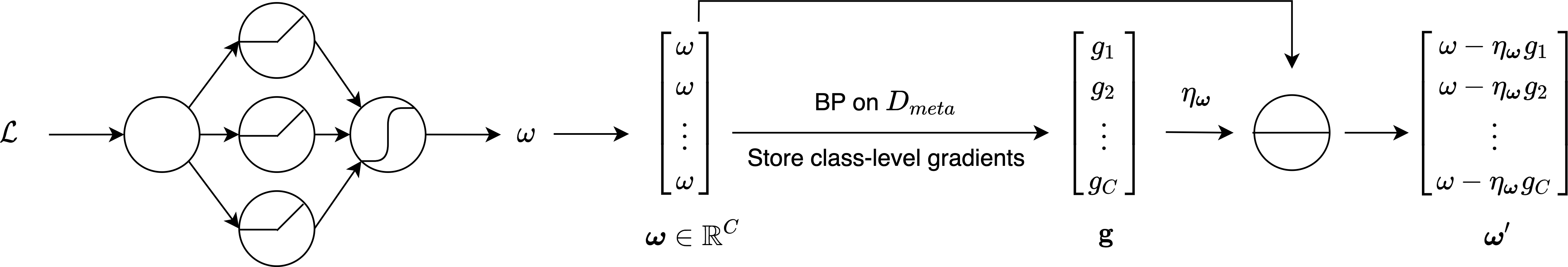
Figure 2: Two-stage Weight Generation. "BP" denotes the back-propagation in Step 2 of the bi-level optimization framework. $\mathbf{g}$ denotes the intermediate gradients w.r.t. $\bm{\omega}$. $\ominus$ denotes the minus operator. Note that $\bm{\omega}$ is the first-stage (instance-level) weight and $\bm{\omega}^{\prime}$ is the second-stage (class-level) weight.

Two-stage Weight Generation. To guarantee scalability, we apply the same weighting network in shuMetaWeightNetLearningExplicit2019a to obtain weights. To efficiently train $\bm{\phi}$ and $\bm{\theta}$, we also adopt the three-step bi-level optimization framework. Moreover, we propose an efficient two-stage scheme embedded in Step 1-3 to generate class-level weights. This process does not introduce any extra computational cost compared to shuMetaWeightNetLearningExplicit2019a . We keep the notations of $\bm{\theta}_{\tau}$ and $\bm{\phi}_{\tau}$ unchanged.

The first stage is embedded in Step 1. Explicitly, we obtain the first-stage class-level weights $\bm{\omega}_{i}=\omega_{i}\bm{1}$, by cloning the output of the weighting network for $C$ times. Then we leverage the cloned weights $\bm{\omega}_{i}$ to manipulate gradients and update $\bm{\theta}$ with a mini-batch of training instances:

$$\hat{\bm{\theta}}_{\tau}\left(\bm{\phi}_{\tau-1}\right)\leftarrow\bm{\theta}_{\tau-1}-\eta_{\bm{\theta}}\frac{1}{n}\sum_{i=1}^{n}f_{\bm{\omega}_{i}\left(\bm{\phi}_{\tau-1}\right)}\left(\nabla_{\bm{\theta}}l_{train}(x_{i},y_{i};\bm{\theta}_{\tau-1})\right),$$ (9)

where $n$ is the mini-batch size, $\eta_{\bm{\theta}}$ is the learning rate of $\bm{\theta}$, and $f_{\bm{\omega}_{i}\left(\bm{\phi}_{\tau-1}\right)}(\cdot)$ is the gradient manipulation operation defined in Eq. (2).

The second stage is embedded in Step 2 and Step 3. Specifically in Step 2, GDW optimizes $\bm{\phi}$ with a mini-batch meta set:

$$\bm{\phi}_{\tau}\leftarrow\bm{\phi}_{\tau-1}-\eta_{\bm{\phi}}\frac{1}{m}\sum_{i=1}^{m}\nabla_{\bm{\phi}_{\tau-1}}l_{meta}(x_{i}^{v},y_{i}^{v};\hat{\bm{\theta}}_{\tau}(\bm{\phi}_{\tau-1})),$$ (10)

where $m$ is the mini-batch size and $\eta_{\bm{\phi}}$ is the learning rate of $\bm{\phi}$. During the back-propagation in updating $\bm{\phi}_{\tau}$, GDW generates the second-stage weights using the intermediate gradients $\mathbf{g}_{i}$ on $\bm{\omega}_{i}$. Precisely,

$$\bm{\omega}^{\prime}_{i}=\bm{\omega}_{i}-\eta_{\bm{\omega}}\rm{clip}(\frac{\mathbf{g_{i}}}{\|\mathbf{g_{i}}\|_{1}},-c,c),$$ (11)

where $\mathbf{g_{i}}$ represents $\frac{1}{m}\sum_{i=1}^{m}\nabla_{\bm{\omega}_{i}}l_{meta}(x_{i}^{v},y_{i}^{v};\hat{\bm{\theta}}_{\tau}(\bm{\phi}_{\tau-1}))$ and $c=0.2$ denotes the clip parameter. Then we impose the zero-mean constraint proposed in Eq. (4) on $\bm{\omega}^{\prime}_{i}$, which is later used in Step 3 to update $\bm{\theta}_{\tau-1}$. Note that the two-stage weight generation scheme does not introduce any extra computational cost compared to MWNet because this generation process only utilizes the intermediate gradients during the back-propagation. In Step 3, we use $\bm{\omega}^{\prime}_{i}$ to manipulate gradients and update the model parameters $\bm{\theta}_{\tau-1}$:

$$\bm{\theta}_{\tau}\leftarrow\bm{\theta}_{\tau-1}-\eta_{\bm{\theta}}\frac{1}{n}\sum_{i=1}^{n}f_{\bm{\omega}^{\prime}_{i}}\left(\nabla_{\bm{\theta}}l_{train}(x_{i},y_{i};\bm{\theta}_{\tau-1})\right).$$ (12)

The only difference between Step 1 and Step 3 is that we use $\bm{\omega}^{\prime}_{i}$ instead of the cloned output of the weighting network $\bm{\omega}_{i}$ to optimize $\bm{\theta}$. Since we only introduce $\bm{\phi}$ as extra learnable parameters, GDW can scale to large datasets. We summarize GDW in Algorithm 1. Moreover, we visualize the two-stage weight generation process in Figure 2 for better demonstration.

Algorithm 1 Generalized Data Weighting via Class-Level Gradients Manipulation

Input: Training set: $D_{train}$, Meta set: $D_{meta}$, batch size $n,m$, # of iterations $T$
      Initial model parameters: $\bm{\theta}_{0}$, initial weighting network parameters: $\bm{\phi}_{0}$
      Output: Trained model: $\bm{\theta}_{T}$

1for $\tau\leftarrow 1$ to $T$ do

2     $\{x_{i},y_{i}\}_{i=1}^{n}\leftarrow$ SampleFrom$(D_{train})$

3     $\{x_{i}^{v},y_{i}^{v}\}_{i=1}^{m}\leftarrow$ SampleFrom$(D_{meta})$

4     Generate $\bm{\omega}_{i}$ from $\mathcal{L}_{i}$ via the weighting network parameterized by $\bm{\phi}_{\tau-1}$

5     Manipulate gradients by Eq. (2) and update $\hat{\bm{\theta}}_{\tau}$ by Eq. (9)

6     Update $\bm{\phi}_{\tau}$ by Eq. (10);

7     Update $\bm{\omega}_{i}$ to $\bm{\omega}^{\prime}_{i}$ by Eq. (11) and constrain $\bm{\omega}^{\prime}_{i}$ by Eq. (4)

8     Manipulate gradients with $\bm{\omega}^{\prime}_{i}$ by Eq. (2) and update $\bm{\theta}_{\tau}$ by Eq. (12)

4 Experiments

We conduct extensive experiments on classification tasks to examine the performance of GDW. We compare GDW with other methods in the label noise setting and class imbalance setting in Section 4.1 and Section 4.2, respectively. Next, we perform experiments on the real-world dataset Clothing1M tongxiaoLearningMassiveNoisy2015 in Section 4.3. We conduct further experiments to verify the performance of GDW in the mixed setting, i.e. the coexistence of label noise and class imbalance (see Appendix F for details).

4.1 Label Noise Setting

Setup. Following shuMetaWeightNetLearningExplicit2019a , we study two settings of label noise: a) Uniform noise: every instance’s label uniformly flips to other class labels with probability $p$; b) Flip noise: each class randomly flips to another class with probability $p$. Note that the probability $p$ represents the noise ratio. We randomly select $100$ clean images per class from CIFAR10 krizhevskyLearningMultipleLayers2009 as the meta set ($1000$ images in total). Similarly, we select a total of $1000$ images from CIFAR100 as its meta set. We use ResNet-32 heDeepResidualLearning2016 as the classifier model.

Comparison methods. We mainly compare GDW with meta-learning methods: 1) L2RW renLearningReweightExamples2018 , which assigns weights to instances based on gradient directions; 2) INSW huLearningDataManipulation2019a , which derives instance weights adaptively from the meta set; 3) MWNet shuMetaWeightNetLearningExplicit2019a ; 4) Soft-label vyasLearningSoftLabels2020b , which learns a label smoothing parameter for every instance; 5) Gen-label alganMetaSoftLabel2021a , which generates a meta-soft-label for every instance. We also compare GDW with some traditional methods: 6) BaseModel, which trains ResNet-32 on the noisy training set; 7) Fine-tuning, which uses the meta set to fine-tune the trained model in BaseModel; 8) Co-teaching hanCoteachingRobustTraining2018a ; 9) GLC hendrycksUsingTrustedData2018 .

Training. Most of our training settings follow shuMetaWeightNetLearningExplicit2019a and we use the cosine learning rate decay schedule loshchilovSGDRStochasticGradient2016 for a total of $80$ epochs for all methods. See Appendix C for details.

Table 2: Test accuracy on CIFAR10 and CIFAR100 with different uniform noise ratios.

Dataset	CIFAR10			CIFAR100
	$0\%$	$40\%$	$60\%$	$0\%$	$40\%$	$60\%$
BaseModel	$92.73\pm 0.37$	$84.38\pm 0.32$	$77.92\pm 0.29$	$70.42\pm 0.54$	$57.28\pm 0.80$	$46.86\pm 1.54$
Fine-tuning	$92.77\pm 0.37$	$84.73\pm 0.47$	$78.41\pm 0.31$	$70.52\pm 0.57$	$57.38\pm 0.87$	$47.06\pm 1.47$
Co-teaching	$91.54\pm 0.39$	$85.26\pm 0.56$	$78.90\pm 6.64$	$68.33\pm 0.13$	$59.58\pm 0.83$	$37.74\pm 2.60$
GLC	$90.85\pm 0.22$	$86.12\pm 0.54$	$81.55\pm 0.60$	$65.05\pm 0.59$	$56.99\pm 0.82$	$41.74\pm 1.98$
L2RW	$89.70\pm 0.50$	$84.66\pm 1.21$	$79.98\pm 1.18$	$63.40\pm 1.31$	$47.06\pm 4.84$	$36.02\pm 2.17$
INSW	$92.70\pm 0.57$	$84.88\pm 0.64$	$78.77\pm 0.82$	$70.52\pm 0.39$	$57.11\pm 0.66$	$48.00\pm 1.16$
MWNet	92.95 $\pm$ 0.33	$86.46\pm 0.31$	$81.14\pm 0.94$	$\textbf{70.64}\pm\textbf{0.31}$	$58.37\pm 0.33$	$50.21\pm 2.98$
Soft-label	$92.63\pm 0.27$	$86.52\pm 0.10$	$80.94\pm 0.25$	$70.50\pm 0.44$	$57.48\pm 0.43$	$48.18\pm 0.89$
Gen-label	$92.56\pm 0.56$	$84.68\pm 0.57$	$78.32\pm 0.94$	$70.46\pm 0.37$	$57.86\pm 0.50$	$48.08\pm 0.98$
GDW	92.94 $\pm$ 0.15	88.14 $\pm$ 0.35	84.11 $\pm$ 0.21	70.65 $\pm$ 0.52	59.82 $\pm$ 1.62	53.33 $\pm$ 3.70

Table 3: Test accuracy on CIFAR10 and CIFAR100 with different flip noise ratios.

Dataset	CIFAR10			CIFAR100
	$0\%$	$20\%$	$40\%$	$0\%$	$20\%$	$40\%$
BaseModel	$92.73\pm 0.37$	$90.14\pm 0.35$	$81.20\pm 0.93$	$70.42\pm 0.54$	$64.96\pm 0.16$	$49.83\pm 0.82$
Fine-tuning	$92.77\pm 0.37$	$90.15\pm 0.36$	$81.53\pm 0.96$	$70.52\pm 0.57$	$65.02\pm 0.22$	$50.23\pm 0.71$
Co-teaching	$91.54\pm 0.39$	$89.27\pm 0.24$	$69.77\pm 3.97$	$68.33\pm 0.13$	$62.96\pm 0.73$	$42.54\pm 1.68$
GLC	$90.85\pm 0.22$	$90.22\pm 0.13$	89.74 $\pm$ 0.19	$65.05\pm 0.59$	$64.11\pm 0.40$	63.11 $\pm$ 0.93
L2RW	$89.70\pm 0.50$	$88.21\pm 0.49$	$82.90\pm 1.27$	$63.40\pm 1.31$	$55.27\pm 2.27$	$45.41\pm 2.53$
INSW	$92.70\pm 0.57$	$89.90\pm 0.45$	$80.09\pm 2.00$	$70.52\pm 0.39$	$65.32\pm 0.27$	$50.13\pm 0.39$
MWNet	92.95 $\pm$ 0.33	$89.93\pm 0.17$	$85.55\pm 0.82$	$\textbf{70.64}\pm\textbf{0.31}$	$64.72\pm 0.68$	$50.62\pm 0.46$
Soft-label	$92.63\pm 0.27$	$90.17\pm 0.47$	$85.52\pm 0.78$	$70.50\pm 0.44$	$65.20\pm 0.45$	$50.97\pm 0.41$
Gen-label	$92.56\pm 0.56$	$90.18\pm 0.13$	$80.93\pm 1.29$	$70.46\pm 0.37$	$64.94\pm 0.53$	$49.93\pm 0.55$
GDW	92.94 $\pm$ 0.15	91.05 $\pm$ 0.26	$87.70\pm 0.37$	70.65 $\pm$ 0.52	65.41 $\pm$ 0.75	$52.44\pm 0.79$

Analysis. For all experiments, we report the mean and standard deviation over $5$ runs in Table 2 and Table 3, where the best results are in bold and the second-best results are marked by underlines. First, we can observe that GDW outperforms nearly all the competing methods in all noise settings except for the $40\%$ flip noise setting. Under this setting, GLC estimates the label corruption matrix well and thus performs the best, whereas the flip noise assumption scarcely holds in real-world scenarios. Note that GLC also performs much better than MWNet under the $40\%$ flip noise setting as reported in shuMetaWeightNetLearningExplicit2019a . Besides, under all noise settings, GDW has a consistent performance gain compared with MWNet, which aligns with our motivation in Figure 1. Furthermore, as the ratio increases from $40\%$ to $60\%$ in the uniform noise setting, the gap between GDW and MWNet increases from $1.68\%$ to $2.97\%$ in CIFAR10 and $1.45\%$ to $3.12\%$ in CIFAR100. Even under $60\%$ uniform noise, GDW still has low test errors in both datasets and achieves more than $3\%$ gain in CIFAR10 and $6\%$ gain in CIFAR100 compared with the second-best method. Last but not least, GDW outperforms Soft-label and Gen-label in all settings. One possible reason is that manipulating gradient flows is a more direct way to capture class-level information than learning labels.

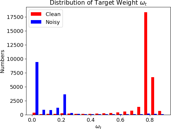
Figure 3: Class-level target weight ($\bm{\omega}_{t}$) distribution on CIFAR10 under $40\%$ uniform noise. $\bm{\omega}_{t}$ of most clean instances are larger than that of most noisy instances, which means $\bm{\omega}_{t}$ can differentiate between clean and noisy instances.

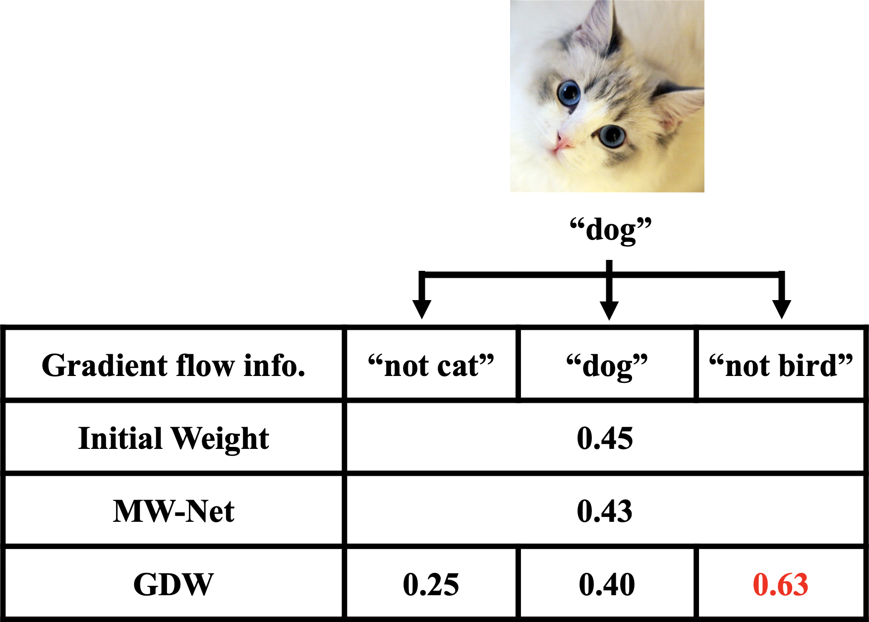
Figure 4: The change of class-level weights in an iteration for a noisy instance (cat mislabeled as "dog"). MWNet downweights all gradient flows. In contrast, GDW upweights the "not bird" gradient flow for better information use.

In Figure 4, we show the distribution of class-level target weight ($\bm{\omega}_{t}$) on clean and noisy instances in one epoch under the CIFAR10 40% uniform noise setting. We observe that $\bm{\omega}_{t}$ of most clean instances are larger than that of most noisy instances, which indicates that $\bm{\omega}_{t}$ can distinguish between clean instances and noisy instances. This is consistent with Eq. (3) that $\bm{\omega}_{t}$ serves as the instance weight.

To better understand the changing trend of non-target class-level weights, we visualize the ratio of increased weights in one epoch in Figure 6 under the CIFAR10 40% uniform noise setting. Specifically, there are three categories: non-target weights on clean instances ($\bm{\omega}^{c}_{nt}$), true target weights on noisy instances ($\bm{\omega}^{n}_{tt}$) and non-target (excluding true targets) weights on noisy instances ($\bm{\omega}^{n}_{nt}$). Formally, "target weight" means the class-level weight on the label position. "true-target weight" means the class-level weight on the true label position, which are only applicable for noisy instances. "non-target weight" means the class-level weight except the label position and the true label position. For example, as shown in Figure 1 where a cat is mislabeled as "dog", the corresponding meanings of the notations are as follows: 1) $\bm{\omega}^{n}_{t}$ means $\bm{\omega}_{dog}$ ("dog" is the target); 2) $\bm{\omega}^{n}_{tt}$ means $\bm{\omega}_{cat}$ ("cat" is the ture target); 3) $\bm{\omega}^{n}_{nt}$ means $\bm{\omega}_{bird}$ ("bird" is one of the non-targets). For a correctly labeled cat, the corresponding meanings are: 1) $\bm{\omega}^{c}_{t}=\bm{\omega}^{c}_{tt}$ means $\bm{\omega}_{cat}$ ("cat" is both the target and the ture target); 2) $\bm{\omega}^{c}_{nt}$ means $\bm{\omega}_{dog}$ and $\bm{\omega}_{bird}$ ("dog" and "bird" are both non-targets).

Note that in Figure 1, $\bm{\omega}^{n}_{tt}$ represents the importance of the "not cat" gradient flow and $\bm{\omega}^{n}_{nt}$ represents the importance of the "not bird" gradient flow. If the cat image in Figure 1 is correctly labeled as "cat", then the two non-target weights $\bm{\omega}^{c}_{nt}$ are used to represent the importance of the "not dog" and the "not bird" gradient flows, respectively. In one epoch, we calculate the ratios of the number of increased $\bm{\omega}^{c}_{nt}$, $\bm{\omega}^{n}_{tt}$ and $\bm{\omega}^{n}_{nt}$ to the number of all corresponding weights. $\bm{\omega}^{c}_{nt}$ and $\bm{\omega}^{n}_{nt}$ are expected to increase since their gradient flows contain valuable information, whereas $\bm{\omega}^{n}_{tt}$ is expected to decrease because the "not cat" gradient flow contains harmful information. Figure 6 aligns perfectly with our expectation. Note that the lines of $\bm{\omega}^{c}_{nt}$ and $\bm{\omega}^{n}_{nt}$ nearly coincide with each other and fluctuate around $65\%$. This means non-target weights on clean instances and noisy instances share the same changing pattern, i.e., around $65\%$ of $\bm{\omega}^{c}_{nt}$ and $\bm{\omega}^{n}_{nt}$ increase. Besides, less than $20\%$ of $\bm{\omega}^{n}_{tt}$ increase and thus more than $80\%$ decrease, which means the gradient flows of $\bm{\omega}^{n}_{tt}$ contain much harmful information.

In Figure 4, we show the change of class-level weights in an iteration for a noisy instance, i.e., a cat image mislabeled as "dog". The gradient flows of "not cat" and "dog" contain harmful information and thus are downweighted by GDW. In addition, GDW upweights the valuable "not bird" gradient flow from $0.45$ to $0.63$. By contrast, unable to capture class-level information, MWNet downweights all gradient flows from $0.45$ to $0.43$, which leads to information loss on the "not bird" gradient flow.

Training without the zero-mean constraint. We have also tried training without the zero-mean constraint in Section 3.3 and got poor results (see Appendix B.2 for details). Denote the true target as $tt$ and one of the non-target labels as $nt$ ($nt\neq tt$). Note that the gradient can be unrolled as (see Appendix B.2 for details):

$$f_{\bm{\omega}}\left(\nabla_{\bm{\theta}}\mathcal{L}\right)=\bm{\omega}_{t}\sum_{j}\left({\bm{p}^{\prime}_{j}}-\mathbf{y}_{j}\right)\frac{\partial\bm{l}_{j}}{\partial\bm{\theta}}+\left(\sum_{k}{{\bm{\omega}_{k}}{\bm{p}_{k}}}-\bm{\omega}_{t}\right)\sum_{j}{\bm{p}^{\prime}_{j}}\frac{\partial\bm{l}_{j}}{\partial\bm{\theta}}.$$ (13)

If $\sum_{k}{{\bm{\omega}_{k}}{\bm{p}_{k}}}-\bm{\omega}_{t}$ is positive and the learning rate is small enough, $\left(\sum_{k}{{\bm{\omega}_{k}}{\bm{p}_{k}}}-\bm{\omega}_{t}\right)\bm{p}^{\prime}_{tt}\frac{\partial\bm{l}_{tt}}{\partial\bm{\theta}}$ contributes to the decrease of the true target logit $\bm{l}_{tt}$ after a gradient descent step. If negative, $\left(\sum_{k}{{\bm{\omega}_{k}}{\bm{p}_{k}}}-\bm{\omega}_{t}\right)\bm{p}^{\prime}_{nt}\frac{\partial\bm{l}_{nt}}{\partial\bm{\theta}}$ contributes to the increase of the non-target logit $\bm{l}_{nt}$. Therefore, without the zero-mean constraint, the second term in Eq. (13) may hurt the performance of the model regardless of the sign of $\sum_{k}{{\bm{\omega}_{k}}{\bm{p}_{k}}}-\bm{\omega}_{t}$. Similarly, training without the constraint results in poor performance in other settings. Hence we omit those results in the following subsections.

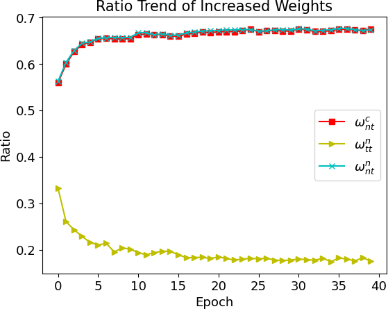
Figure 5: Ratio trend of the number of increased $\bm{\omega}^{c}_{nt}$, $\bm{\omega}^{n}_{tt}$, and $\bm{\omega}^{n}_{nt}$ under the CIFAR10 40% uniform noise setting. Around $65\%$ of $\bm{\omega}^{c}_{nt}$ and $\bm{\omega}^{n}_{nt}$ increase since they contain useful information. Besides, less than $20\%$ of $\bm{\omega}^{n}_{tt}$ increase and thus more than $80\%$ of $\bm{\omega}^{n}_{tt}$ decrease since they contain harmful information.

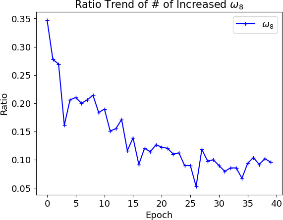
Figure 6: Ratio trend of the number of increased $\bm{\omega}_{8}$ on $C9$ instances under the Long-Tailed CIFAR10 $\mu=0.1$ setting. Less than $10\%$ of $\bm{\omega}_{8}$ increase and thus more than $90\%$ decrease. A small $\bm{\omega}_{8}$ strikes a balance between two kinds of information: "$C8$" and "not $C8$", which better handles class imbalance.

4.2 Class Imbalance Setting

Table 4: Test accuracy on the long-tailed CIFAR10 and CIFAR100 with different imbalance ratios.

Dataset	CIFAR10			CIFAR100
	$\mu=1$	$\mu=0.1$	$\mu=0.01$	$\mu=1$	$\mu=0.1$	$\mu=0.01$
BaseModel	$92.73\pm 0.37$	$85.93\pm 0.57$	$69.77\pm 1.13$	$70.42\pm 0.54$	$56.25\pm 0.49$	$37.79\pm 0.82$
Fine-tuning	$92.77\pm 0.37$	$82.60\pm 0.49$	$59.76\pm 1.00$	$70.52\pm 0.57$	$55.95\pm 0.50$	$37.10\pm 0.87$
Focal	$91.68\pm 0.49$	$84.57\pm 0.83$	$65.78\pm 4.02$	$68.48\pm 0.38$	$55.02\pm 0.51$	$37.43\pm 1.00$
Balanced	$92.80\pm 0.47$	$86.05\pm 0.46$	$63.63\pm 3.60$	$70.56\pm 0.56$	$55.02\pm 0.80$	$27.60\pm 1.39$
L2RW	$89.70\pm 0.50$	$79.11\pm 3.40$	$51.15\pm 7.13$	$63.40\pm 1.31$	$46.28\pm 4.51$	$25.86\pm 5.78$
INSW	$92.70\pm 0.57$	$86.31\pm 0.28$	$70.27\pm 0.24$	$70.52\pm 0.39$	$55.94\pm 0.51$	$37.67\pm 0.59$
MWNet	92.95 $\pm$ 0.33	$86.17\pm 0.75$	$62.70\pm 1.76$	$\textbf{70.64}\pm\textbf{0.31}$	$56.49\pm 1.52$	$37.83\pm 0.86$
GDW	92.94 $\pm$ 0.15	86.77 $\pm$ 0.55	71.31 $\pm$ 1.03	70.65 $\pm$ 0.52	56.78 $\pm$ 0.52	37.94 $\pm$ 1.58

Setup and comparison methods. The imbalance factor $\mu\in(0,1)$ of a dataset is defined as the number of instances in the smallest class divided by that of the largest shuMetaWeightNetLearningExplicit2019a . Long-Tailed CIFAR krizhevskyLearningMultipleLayers2009 are created by reducing the number of training instances per class according to an exponential function $n=n_{i}\mu^{i/(C-1)}$, where $i$ is the class index (0-indexed) and $n_{i}$ is the original number of training instances. Comparison methods include: 1) L2RW renLearningReweightExamples2018 ; 2) INSW huLearningDataManipulation2019a ; 3) MWNet shuMetaWeightNetLearningExplicit2019a ; 4) BaseModel; 5) Fine-tuning; 6) Balanced cuiClassBalancedLossBased2019 ; 7) Focal linFocalLossDense2020 .

Analysis. As shown in Table 4, GDW performs best in nearly all settings and exceeds MWNet by $8.6\%$ when the imbalance ratio $\mu$ is $0.01$ in CIFAR10. Besides, INSW achieves competitive performance at the cost of introducing a huge amount of learnable parameters (equal to the training dataset size $N$). Furthermore, we find that BaseModel achieves competitive performance, but fine-tuning on the meta set hurts the model’s performance. We have tried different learning rates from $10^{-7}$ to $10^{-1}$ for fine-tuning, but the results are similar. One explanation is that the balanced meta set worsens the model learned from the imbalanced training set. These results align with the experimental results in huLearningDataManipulation2019a which also deals with class imbalance.

Denote the smallest class as $C9$ and the second smallest class as $C8$ in Long-Tailed CIFAR10 with $\mu=0.1$. Recall that $\bm{\omega}_{j}$ denotes the $j^{th}$ class-level weight. For all $C9$ instances in an epoch, we calculate the ratio of the number of increased $\bm{\omega}_{8}$ to the number of all $\bm{\omega}_{8}$, and then visualize the ratio trend in Figure 6. Since $C9$ is the smallest class, instance weighting methods upweight both $\bm{\omega}_{8}$ and $\bm{\omega}_{9}$ on a $C9$ instance. Yet in Figure 6, less than $10\%$ of $\bm{\omega}_{8}$ increase and thus more than $90\%$ decrease. This can be explained as follows. There are two kinds of information in the long-tailed dataset regarded to $C8$: "$C8$" and "not $C8$". Since $C8$ belongs to the minority class, the dataset is biased towards the "not $C8$" information. Because $\bm{\omega}_{8}$ represents the importance of "not $C8$", a smaller $\bm{\omega}_{8}$ weakens the "not $C8$" information. As a result, decreased $\bm{\omega}_{8}$ achieves a balance between two kinds of information: "$C8$" and "not $C8$", thus better handling class imbalance at the class level. We have conducted further experiments on imbalanced settings to verify the effectiveness of GDW and see Appendix D for details.

4.3 Real-world Setting

Setup and training. The Clothing1M dataset contains one million images from fourteen classes collected from the web tongxiaoLearningMassiveNoisy2015 . Labels are constructed from surrounding texts of images and thus contain some errors. We use the ResNet-18 model pre-trained on ImageNet dengImageNetLargescaleHierarchical2009 as the classifier. The comparison methods are the same as those in the label noise setting since the main issue of Clothing1M is label noise tongxiaoLearningMassiveNoisy2015 . All methods are trained for $5$ epochs via SGD with a $0.9$ momentum, a $10^{-3}$ initial learning rate, a $10^{-3}$ weight decay, and a $128$ batchsize. See Appendix E for details.

Table 5: Test accuracy on Clothing1M.

Method	BaseModel	Fine-tuning	Co-teaching	GLC	L2RW	INSW	MWNet	Soft-label	Gen-label	GDW
Accuracy($\%$)	$65.02$	$67.68$	$68.13$	$68.60$	$68.80$	$68.25$	$68.46$	$68.69$	$67.64$	69.39

Analysis. As shown in Table 5, GDW achieves the best performance among all the comparison methods and outperforms MWNet by $0.93\%$. In contrast to unsatisfying results in previous settings, L2RW performs quite well in this setting. One possible explanation is that, compared with INSW and MWNet which update weights iteratively, L2RW obtains instance weights only based on current gradients. As a result, L2RW can more quickly adapt to the model’s state, but meanwhile suffers from unstable weights shuMetaWeightNetLearningExplicit2019a . In previous settings, we train models from scratch, which need stable weights to stabilize training. Therefore, INSW and MWNet generally achieve better performance than L2RW. Whereas in this setting, we use the pre-trained ResNet-18 model which is already stable enough. Thus L2RW performs better than INSW and MWNet.

5 Conclusion

Many instance weighting methods have recently been proposed to tackle label noise and class imbalance, but they cannot capture class-level information. For better information use when handling the two issues, we propose GDW to generalize data weighting from instance level to class level by reweighting gradient flows. Besides, to efficiently obtain class-level weights, we design a two-stage weight generation scheme which is embedded in a three-step bi-level optimization framework and leverages intermediate gradients to update class-level weights via a gradient descent step. In this way, GDW achieves remarkable performance improvement in various settings.

The limitations of GDW are two-fold. Firstly, the gradient manipulation is only applicable to single-label classification tasks. When applied to multi-label tasks, the formulation of gradient manipulation need some modifications. Secondly, GDW does not outperform comparison methods by a large margin in class imbalance settings despite the potential effectiveness analyzed in Section 4.2. One possible explanation is that better information utilization may not result in performance gain which also depends on various other factors.

6 Acknowledgement

We thank Prof. Hao Zhang from Tsinghua University for helpful suggestions. This research was supported in part by the MSR-Mila collaboration funding. Besides, this research was empowered in part by the computational support provided by Compute Canada (www.computecanada.ca).

Appendix A Derivation of D1

Denote the logit vector as $\bm{x}$, we have

$$\bm{p}_{j}= \frac{e^{\bm{x}_{j}}}{\sum_{k}e^{\bm{x}_{k}}}$$ (14)

$$\mathcal{L}= -\sum_{j}\bm{y}_{j}\log{\bm{p}_{j}}.$$ (15)

For the target (label) position $t$ we have $\bm{y}_{t}=1$ and

$$\frac{\partial\mathcal{L}}{\partial\bm{x}_{t}}=\frac{\partial\mathcal{L}}{\partial\bm{p}_{t}}\frac{\partial\bm{p}_{t}}{\partial\bm{x}_{t}}=-\frac{\sum_{k}e^{\bm{x}_{k}}}{e^{\bm{x}_{t}}}\frac{e^{\bm{x}_{t}}\sum_{k}e^{\bm{x}_{k}}-e^{2\bm{x}_{t}}}{\left(\sum_{k}e^{\bm{x}_{k}}\right)^{2}}=\frac{e^{\bm{x}_{t}}}{\sum_{k}e^{\bm{x}_{k}}}-1=\bm{p}_{t}-\bm{y}_{t}.$$ (16)

For any other position $j$ ($j\neq t$), we have $\bm{y}_{j}=0$ and

$$\frac{\partial\mathcal{L}}{\partial\bm{x}_{j}}=\frac{\partial\mathcal{L}}{\partial\bm{p}_{t}}\frac{\partial\bm{p}_{t}}{\partial\bm{x}_{j}}=-\frac{\sum_{k}e^{\bm{x}_{k}}}{e^{\bm{x}_{t}}}\frac{-e^{\bm{x}_{j}+\bm{x}_{t}}}{\left(\sum_{k}e^{\bm{x}_{k}}\right)^{2}}=\frac{e^{\bm{x}_{j}}}{\sum_{k}e^{\bm{x}_{k}}}=\bm{p}_{j}-\bm{y}_{j}.$$ (17)

Therefore, we can conclude that $\bm{D}_{1}$ = $\bm{p}-\bm{y}$.

Appendix B Zero-mean Constraint on Class-level Weights

B.1 Derivation

$$\bm{\omega}_{j}(\bm{p}_{j}-\mathbf{y}_{j})= \bm{\omega}_{j}\bm{p}_{j}-\bm{\omega}_{j}\mathbf{y}_{j}$$ (18)

$$= \left(\sum_{k}\bm{\omega}_{k}\bm{p}_{k}\right)\frac{\bm{\omega}_{j}\bm{p}_{j}}{\sum_{k}\bm{\omega}_{k}\bm{p}_{k}}-\left(\sum_{k}\bm{\omega}_{k}\mathbf{y}_{k}\right)\frac{\bm{\omega}_{j}\mathbf{y}_{j}}{\sum_{k}\bm{\omega}_{k}\mathbf{y}_{k}}$$ (19)

If $$\mathbf{y}_{j}=0 0 \bm{\omega}_{t}\mathbf{y}_{j}$$, the second term of (19) becomes , therefore can be rewritten as

$$= \left(\sum_{k}\bm{\omega}_{k}\bm{p}_{k}\right){\bm{p}^{\prime}_{j}}-\bm{\omega}_{t}\mathbf{y}_{j}$$ (20)

$$= \bm{\omega}_{t}\left({\bm{p}^{\prime}_{j}}-{\mathbf{y}_{j}}\right)+\left(\sum_{k}{{\bm{\omega}_{k}}{\bm{p}_{k}}}-\bm{\omega}_{t}\right){\bm{p}^{\prime}_{j}}.$$ (21)

B.2 Training without Zero-mean Constraint

$$\begin{split}f_{\bm{\omega}}\left(\nabla_{\bm{\theta}}\mathcal{L}\right)=&f_{\bm{\omega}}(\sum_{j}\frac{\partial\mathcal{L}_{i}}{\partial\bm{l}_{j}}\frac{\partial\bm{l}_{j}}{\partial\bm{\theta}})\\ =&\sum_{j}\bm{\omega}_{j}(\bm{p}_{j}-\mathbf{y}_{j})\frac{\partial\bm{l}_{j}}{\partial\bm{\theta}}\\ =&\bm{\omega}_{t}\sum_{j}({\bm{p}^{\prime}_{j}}-\mathbf{y}_{j})\frac{\partial\bm{l}_{j}}{\partial\bm{\theta}}+(\sum_{k}{{\bm{\omega}_{k}}{\bm{p}_{k}}}-\bm{\omega}_{t})\sum_{j}{\bm{p}^{\prime}_{j}}\frac{\partial\bm{l}_{j}}{\partial\bm{\theta}}.\end{split}$$ (22)

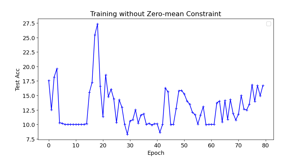
Figure 7: Training curve without zero-mean constraint on CIFAR10 under 40% uniform noise.

Without zero-mean constraint, the training becomes unstable. We plot the training curve of the CIFAR10 40% uniform noise setting in Figure 7.

Appendix C Label Noise Training Setting

Following the training setting of shuMetaWeightNetLearningExplicit2019a , the classifier network is trained with SGD with a weight decay $5$e-$4$, an initial learning rate of $1$e-$1$ and a mini-batch size of $100$ for all methods. We use the cosine learning rate decay schedule loshchilovSGDRStochasticGradient2016 for a total of 80 epochs. The MLP weighting network is trained with Adam kingmaAdamMethodStochastic2015 with a fixed learning rate 1e-3 and a weight decay 1e-4. For GLC, we first train 40 epochs to estimate the label corruption matrix and then train another 40 epochs to evaluate its performance. Since Co-teach uses two models, each model is trained for 40 epochs for a fair comparison. We repeat every experiment 5 times with different random seeds (seed=1, 10, 100, 1000, 10000, respectively) for network initialization and label noise generation. We report the average test accuracy over the last 5 epochs as the model’s final performance. We use one V100 GPU for all the experiments.

Appendix D Further Experiments on Imbalanced Setting

D.1 Class-level Weight Analysis

We conduct one more experiment under the imbalance setting to better verify the interpretability of GDW. As shown in Table 6, we report the ratio of the number of increased $\bm{\omega}_{i}$ after gradient update on $C_{j}$ instances in one epoch, where $C_{0}$ is the largest class and $C_{9}$ is the smallest class.

Note that $\bm{\omega}_{i}$ on $C_{i}$ contains the "is $C_{i}$" information in the dataset. As a result, $\bm{\omega}_{i}$ on $C_{i}$ should be large for small classes and small for large classes. As shown above, the ratio of increased $\bm{\omega}_{i}$ on $C_{i}$ (the diagonal elements) increases from $0.036$ to $0.935$ as $i$ increases from $0$ to $9$.

On the other hand, $\bm{\omega}_{i}$ on $C_{j}$ ($j\neq i$) contains the "not $C_{i}$" information in the dataset. If $i$ is a large class, $\bm{\omega}_{i}$ on $C_{j}$ ($j\neq i$) should be large and vice versa. For $\bm{\omega}_{i}$ ($i=0,1,2,3,4$), the ratio of increased $\bm{\omega}_{i}$ on $C_{j}$ ($j\neq i$) are generally larger than $0.5$, and for $\bm{\omega}_{i}$ ($i=5,6,7,8,9$), the ratio of increased $\bm{\omega}_{i}$ on $C_{j}$ ($j\neq i$) are generally less than $0.5$. These results align with our analysis on the interpretable information of gradient flows.

Table 6: Ratio of increased class-level weights under the imbalance setting.

weight/class	$C_{0}$	$C_{1}$	$C_{2}$	$C_{3}$	$C_{4}$	$C_{5}$	$C_{6}$	$C_{7}$	$C_{8}$	$C_{9}$
$\bm{\omega}_{0}$	0.036	0.968	0.973	0.972	0.965	0.974	0.972	0.976	0.956	0.973
$\bm{\omega}_{1}$	0.887	0.095	0.912	0.929	0.907	0.927	0.911	0.922	0.910	0.920
$\bm{\omega}_{2}$	0.848	0.844	0.141	0.839	0.822	0.845	0.818	0.847	0.829	0.802
$\bm{\omega}_{3}$	0.585	0.608	0.552	0.405	0.569	0.541	0.561	0.559	0.617	0.596
$\bm{\omega}_{4}$	0.474	0.521	0.420	0.460	0.509	0.455	0.456	0.482	0.467	0.512
$\bm{\omega}_{5}$	0.291	0.261	0.288	0.252	0.309	0.701	0.303	0.267	0.297	0.257
$\bm{\omega}_{6}$	0.199	0.189	0.169	0.198	0.196	0.222	0.778	0.195	0.207	0.182
$\bm{\omega}_{7}$	0.117	0.117	0.105	0.084	0.115	0.079	0.126	0.920	0.133	0.090
$\bm{\omega}_{8}$	0.115	0.124	0.178	0.185	0.184	0.174	0.191	0.181	0.862	0.137
$\bm{\omega}_{9}$	0.043	0.050	0.064	0.061	0.074	0.062	0.097	0.069	0.040	0.935

D.2 Experiments on Places-LT

Table 7: Test accuracy on Places-LT.

Method	L2RW	INSW	MW-Net	GDW
Accuracy (%)	$15.08$	$17.80$	$18.08$	19.17

We have conducted experiments on the Places-LT dataset liuLargeScaleLongTailedRecognition2019 and compared GDW with other meta-learning-based methods. For all methods, the weight decay is set to $0.001$ and the batchsize is set to $64$. We adopt a $0.01$ initial learning rate and a cosine learning rate decay policy for $10$ epochs. The weight decay is set to $0.001$. The backbone network is ResNet18 and we use the ImageNet pre-trained model for initialization.

As shown in Table 7, GDW achieves the best performance among all the comparison methods and outperforms MWNet by $1.09\%$. This improvement is larger than that of CIFAR100. The reason is that GDW can manipulate class-level information and thus performs better on the dataset with a larger number of classes ($365$ in Places-LT and $100$ in CIFAR100). Besides, we can observe that L2RW performs the worst and the reason may be that L2RW suffers from unstable weights shuMetaWeightNetLearningExplicit2019a .

Appendix E Real-world Training Setting

Similar to shuMetaWeightNetLearningExplicit2019a , we use the $7$k validation set as the meta set and the origin test set to evaluate the classifier’s final performance. For GLC, we first train $2$ epochs to estimate the label corruption matrix and then train another $3$ epochs to evaluate its performance. Since Co-teach uses two models, each model is trained for $3$ epochs for a fair comparison.

Appendix F Experiments on Mixed Setting

We conduct further experiments to verify the performance of GDW in the mixed setting, i.e. the coexistence of label noise and class imbalance. Specifically, we compare GDW with the mostly second-best method MW-Net shuMetaWeightNetLearningExplicit2019a under the mixed setting of uniform noise and class imbalance on CIFAR10 and CIFAR100. As shown in Table 8, GDW demonstrates great performance gain over MW-Net, which means GDW can simultaneously better tackle both problems.

Table 8: Test accuracy under mixed settings.

Dataset	Noise Ratio	Imb Factor	MW-Net	GDW
CIFAR10	$0.40$	$0.10$	$71.54$	$76.30$
CIFAR10	$0.60$	$0.10$	$61.62$	$70.24$
CIFAR10	$0.40$	$0.01$	$48.04$	$48.53$
CIFAR10	$0.60$	$0.01$	$39.51$	$40.07$
CIFAR100	$0.40$	$0.10$	$36.10$	$38.20$
CIFAR100	$0.60$	$0.10$	$24.80$	$25.40$
CIFAR100	$0.40$	$0.01$	$21.26$	$22.07$
CIFAR100	$0.60$	$0.01$	$12.75$	$14.15$

Appendix G Checklist

1. For all authors…

   1. Do the main claims made in the abstract and introduction accurately reflect the paper’s contributions and scope? [Yes]

   2. Did you describe the limitations of your work? [Yes] The proposed method can only be applied on classification tasks.

   3. Did you discuss any potential negative societal impacts of your work? [N/A]

   4. Have you read the ethics review guidelines and ensured that your paper conforms to them? [Yes]

2. If you are including theoretical results…

   1. Did you state the full set of assumptions of all theoretical results? [Yes] See Section 3.

   2. Did you include complete proofs of all theoretical results? [Yes] See Section 3.

3. If you ran experiments…

   1. Did you include the code, data, and instructions needed to reproduce the main experimental results (either in the supplemental material or as a URL)? [Yes] We only use public datasets and the code is in the supplementary materials.

   2. Did you specify all the training details (e.g., data splits, hyperparameters, how they were chosen)? [Yes] Most of our settings follow shuMetaWeightNetLearningExplicit2019a and other details are in the appendix.

   3. Did you report error bars (e.g., with respect to the random seed after running experiments multiple times)? [Yes] We repeat all experiments on CIFAR10 and CIFAR100 with five different seeds and the mean and standard deviation are reported. For the Clothing1M dataset, we only run one experiment due to limited resources.

   4. Did you include the total amount of compute and the type of resources used (e.g., type of GPUs, internal cluster, or cloud provider)? [Yes] We use one V100 GPU. See the appendix for details.

4. If you are using existing assets (e.g., code, data, models) or curating/releasing new assets…

   1. If your work uses existing assets, did you cite the creators? [Yes] For dataset, we cite the papers of CIFAR datasets and the Clothing1M dataset. For code, we cite heDeepResidualLearning2016 .

   2. Did you mention the license of the assets? [N/A]

   3. Did you include any new assets either in the supplemental material or as a URL? [N/A]

   4. Did you discuss whether and how consent was obtained from people whose data you’re using/curating? [N/A]

   5. Did you discuss whether the data you are using/curating contains personally identifiable information or offensive content? [N/A]

5. If you used crowdsourcing or conducted research with human subjects…

   1. Did you include the full text of instructions given to participants and screenshots, if applicable? [N/A]

   2. Did you describe any potential participant risks, with links to Institutional Review Board (IRB) approvals, if applicable? [N/A]

   3. Did you include the estimated hourly wage paid to participants and the total amount spent on participant compensation? [N/A]

References

- (1) Hwanjun Song, Minseok Kim, Dongmin Park, Yooju Shin, and Jae-Gil Lee. Learning from Noisy Labels with Deep Neural Networks: A Survey. arXiv:2007.08199 [cs, stat], June 2021.
- (2) Haibo He and Edwardo A. Garcia. Learning from Imbalanced Data. IEEE Transactions on Knowledge and Data Engineering, 21(9):1263–1284, September 2009.
- (3) Nancy E. ElHady and Julien Provost. A Systematic Survey on Sensor Failure Detection and Fault-Tolerance in Ambient Assisted Living. Sensors, 18(7):1991, July 2018.
- (4) Tong Xiao, Tian Xia, Yi Yang, Chang Huang, and Xiaogang Wang. Learning from massive noisy labeled data for image classification. In 2015 IEEE Conference on Computer Vision and Pattern Recognition (CVPR), pages 2691–2699, Boston, MA, USA, June 2015. IEEE.
- (5) Görkem Algan and İlkay Ulusoy. Label Noise Types and Their Effects on Deep Learning. arXiv:2003.10471 [cs], March 2020.
- (6) Xingquan Zhu and Xindong Wu. Class Noise vs. Attribute Noise: A Quantitative Study. Artificial Intelligence Review, 22(3):177–210, November 2004.
- (7) Benoit Frenay and Michel Verleysen. Classification in the Presence of Label Noise: A Survey. IEEE Transactions on Neural Networks and Learning Systems, 25(5):845–869, May 2014.
- (8) Qiuye Zhao and Mitch Marcus. Long-Tail Distributions and Unsupervised Learning of Morphology. In Proceedings of COLING 2012, pages 3121–3136, Mumbai, India, December 2012. The COLING 2012 Organizing Committee.
- (9) Grant Van Horn and Pietro Perona. The Devil is in the Tails: Fine-grained Classification in the Wild. arXiv:1709.01450 [cs], September 2017.
- (10) Reyes Pavón, Rosalía Laza, Miguel Reboiro-Jato, and Florentino Fdez-Riverola. Assessing the Impact of Class-Imbalanced Data for Classifying Relevant/Irrelevant Medline Documents. In Miguel P. Rocha, Juan M. Corchado Rodríguez, Florentino Fdez-Riverola, and Alfonso Valencia, editors, 5th International Conference on Practical Applications of Computational Biology & Bioinformatics (PACBB 2011), Advances in Intelligent and Soft Computing, pages 345–353, Berlin, Heidelberg, 2011. Springer.
- (11) Harshita Patel, Dharmendra Singh Rajput, G Thippa Reddy, Celestine Iwendi, Ali Kashif Bashir, and Ohyun Jo. A review on classification of imbalanced data for wireless sensor networks. International Journal of Distributed Sensor Networks, 16(4):1550147720916404, April 2020.
- (12) Qi Dong, Shaogang Gong, and Xiatian Zhu. Class Rectification Hard Mining for Imbalanced Deep Learning. In 2017 IEEE International Conference on Computer Vision (ICCV), pages 1869–1878, Venice, October 2017. IEEE.
- (13) Yin Cui, Menglin Jia, Tsung-Yi Lin, Yang Song, and Serge Belongie. Class-Balanced Loss Based on Effective Number of Samples. In 2019 IEEE/CVF Conference on Computer Vision and Pattern Recognition (CVPR), pages 9260–9269, June 2019.
- (14) Saptarshi Sinha, Hiroki Ohashi, and Katsuyuki Nakamura. Class-Wise Difficulty-Balanced Loss for Solving Class-Imbalance. In Hiroshi Ishikawa, Cheng-Lin Liu, Tomas Pajdla, and Jianbo Shi, editors, Computer Vision – ACCV 2020, Lecture Notes in Computer Science, pages 549–565, Cham, 2021. Springer International Publishing.
- (15) Justin M. Johnson and Taghi M. Khoshgoftaar. Survey on deep learning with class imbalance. Journal of Big Data, 6(1):27, March 2019.
- (16) Christian Szegedy, V. Vanhoucke, S. Ioffe, Jonathon Shlens, and Z. Wojna. Rethinking the Inception Architecture for Computer Vision. 2016 IEEE Conference on Computer Vision and Pattern Recognition (CVPR), 2016.
- (17) J. Goldberger and E. Ben-Reuven. Training deep neural-networks using a noise adaptation layer. In International Conference on Learning Representations, 2017.
- (18) Tongliang Liu and Dacheng Tao. Classification with Noisy Labels by Importance Reweighting. IEEE Transactions on Pattern Analysis and Machine Intelligence, 38, November 2014.
- (19) Dan Hendrycks, Mantas Mazeika, Duncan Wilson, and Kevin Gimpel. Using Trusted Data to Train Deep Networks on Labels Corrupted by Severe Noise. In Advances in Neural Information Processing Systems, volume 31. Curran Associates, Inc., 2018.
- (20) Bo Han, Quanming Yao, Xingrui Yu, Gang Niu, Miao Xu, Weihua Hu, Ivor Tsang, and Masashi Sugiyama. Co-teaching: Robust training of deep neural networks with extremely noisy labels. In Advances in Neural Information Processing Systems, volume 31. Curran Associates, Inc., 2018.
- (21) Tsung-Yi Lin, Priya Goyal, Ross Girshick, Kaiming He, and Piotr Dollár. Focal Loss for Dense Object Detection. IEEE Transactions on Pattern Analysis and Machine Intelligence, 42(2):318–327, February 2020.
- (22) Mengye Ren, Wenyuan Zeng, Bin Yang, and Raquel Urtasun. Learning to Reweight Examples for Robust Deep Learning. In Proceedings of the 35th International Conference on Machine Learning, pages 4334–4343. PMLR, July 2018.
- (23) Jun Shu, Qi Xie, Lixuan Yi, Qian Zhao, Sanping Zhou, Zongben Xu, and Deyu Meng. Meta-Weight-Net: Learning an Explicit Mapping For Sample Weighting. In Advances in Neural Information Processing Systems, volume 32. Curran Associates, Inc., 2019.
- (24) Zhiting Hu, Bowen Tan, Russ R Salakhutdinov, Tom M Mitchell, and Eric P Xing. Learning Data Manipulation for Augmentation and Weighting. In Advances in Neural Information Processing Systems, volume 32. Curran Associates, Inc., 2019.
- (25) Xinyi Wang, Hieu Pham, Paul Michel, Antonios Anastasopoulos, Graham Neubig, and J. Carbonell. Optimizing Data Usage via Differentiable Rewards. In International Conference on Machine Learning, 2020.
- (26) Arash Vahdat. Toward Robustness against Label Noise in Training Deep Discriminative Neural Networks. In Advances in Neural Information Processing Systems, volume 30. Curran Associates, Inc., 2017.
- (27) Charles Elkan. The foundations of cost-sensitive learning. In Proceedings of the 17th International Joint Conference on Artificial Intelligence - Volume 2, IJCAI’01, pages 973–978, San Francisco, CA, USA, August 2001. Morgan Kaufmann Publishers Inc.
- (28) Nitesh V. Chawla, Kevin W. Bowyer, Lawrence O. Hall, and W. Philip Kegelmeyer. SMOTE: Synthetic minority over-sampling technique. Journal of Artificial Intelligence Research, 16(1):321–357, June 2002.
- (29) Ashish Anand, Ganesan Pugalenthi, Gary B. Fogel, and P. N. Suganthan. An approach for classification of highly imbalanced data using weighting and undersampling. Amino Acids, 39(5):1385–1391, November 2010.
- (30) Salman H. Khan, Munawar Hayat, Mohammed Bennamoun, Ferdous A. Sohel, and Roberto Togneri. Cost-Sensitive Learning of Deep Feature Representations From Imbalanced Data. IEEE Transactions on Neural Networks and Learning Systems, 29(8):3573–3587, August 2018.
- (31) Bingyi Kang, Saining Xie, Marcus Rohrbach, Zhicheng Yan, Albert Gordo, Jiashi Feng, and Yannis Kalantidis. Decoupling Representation and Classifier for Long-Tailed Recognition. In International Conference on Learning Representations, September 2019.
- (32) Ziwei Liu, Zhongqi Miao, Xiaohang Zhan, Jiayun Wang, Boqing Gong, and Stella X. Yu. Large-Scale Long-Tailed Recognition in an Open World. In 2019 IEEE/CVF Conference on Computer Vision and Pattern Recognition (CVPR), pages 2532–2541, Long Beach, CA, USA, June 2019. IEEE.
- (33) Xudong Wang, Long Lian, Zhongqi Miao, Ziwei Liu, and Stella Yu. Long-tailed Recognition by Routing Diverse Distribution-Aware Experts. In International Conference on Learning Representations, September 2020.
- (34) Brenden M. Lake, Ruslan Salakhutdinov, and Joshua B. Tenenbaum. Human-level concept learning through probabilistic program induction. Science, 350(6266):1332–1338, December 2015.
- (35) Luca Franceschi, Paolo Frasconi, Saverio Salzo, Riccardo Grazzi, and Massimiliano Pontil. Bilevel Programming for Hyperparameter Optimization and Meta-Learning. In Proceedings of the 35th International Conference on Machine Learning, pages 1568–1577. PMLR, July 2018.
- (36) Hanxiao Liu, Karen Simonyan, and Yiming Yang. DARTS: Differentiable Architecture Search. In International Conference on Learning Representations, September 2018.
- (37) Yu-Xiong Wang, Deva Ramanan, and Martial Hebert. Learning to Model the Tail. In Advances in Neural Information Processing Systems, volume 30. Curran Associates, Inc., 2017.
- (38) Lu Jiang, Zhengyuan Zhou, Thomas Leung, Li-Jia Li, and Li Fei-Fei. MentorNet: Learning Data-Driven Curriculum for Very Deep Neural Networks on Corrupted Labels. In Proceedings of the 35th International Conference on Machine Learning, pages 2304–2313. PMLR, July 2018.
- (39) Junnan Li, Yongkang Wong, Qi Zhao, and Mohan S. Kankanhalli. Learning to Learn From Noisy Labeled Data. In 2019 IEEE/CVF Conference on Computer Vision and Pattern Recognition (CVPR), pages 5046–5054, Long Beach, CA, USA, June 2019. IEEE.
- (40) G. Algan and I. Ulusoy. Meta Soft Label Generation for Noisy Labels. 2020 25th International Conference on Pattern Recognition (ICPR), 2021.
- (41) Zizhao Zhang, Han Zhang, Sercan Ö. Arik, Honglak Lee, and Tomas Pfister. Distilling Effective Supervision From Severe Label Noise. In 2020 IEEE/CVF Conference on Computer Vision and Pattern Recognition (CVPR), pages 9291–9300, June 2020.
- (42) Nidhi Vyas, Shreyas Saxena, and Thomas Voice. Learning Soft Labels via Meta Learning. arXiv:2009.09496 [cs, stat], September 2020.
- (43) Shreyas Saxena, Oncel Tuzel, and Dennis DeCoste. Data Parameters: A New Family of Parameters for Learning a Differentiable Curriculum. In Advances in Neural Information Processing Systems, volume 32. Curran Associates, Inc., 2019.
- (44) Andrew G. Howard, Menglong Zhu, Bo Chen, Dmitry Kalenichenko, Weijun Wang, Tobias Weyand, Marco Andreetto, and Hartwig Adam. MobileNets: Efficient Convolutional Neural Networks for Mobile Vision Applications. arXiv:1704.04861 [cs], April 2017.
- (45) Zhenyue Qin, Dongwoo Kim, and Tom Gedeon. Rethinking Softmax with Cross-Entropy: Neural Network Classifier as Mutual Information Estimator. arXiv:1911.10688 [cs, stat], September 2020.
- (46) Shuai Zhao, Liguang Zhou, Wenxiao Wang, Deng Cai, Tin Lun Lam, and Yangsheng Xu. Towards Better Accuracy-efficiency Trade-offs: Divide and Co-training. arXiv:2011.14660 [cs], March 2021.
- (47) A. Krizhevsky. Learning Multiple Layers of Features from Tiny Images. MSc Thesis, University of Toronto, 2009.
- (48) Kaiming He, Xiangyu Zhang, Shaoqing Ren, and Jian Sun. Deep Residual Learning for Image Recognition. In 2016 IEEE Conference on Computer Vision and Pattern Recognition (CVPR), pages 770–778, June 2016.
- (49) Ilya Loshchilov and Frank Hutter. SGDR: Stochastic Gradient Descent with Warm Restarts. International Conference on Learning Representations, November 2016.
- (50) Jia Deng, Wei Dong, Richard Socher, Li-Jia Li, Kai Li, and Li Fei-Fei. ImageNet: A large-scale hierarchical image database. In 2009 IEEE Conference on Computer Vision and Pattern Recognition, pages 248–255, June 2009.
- (51) Diederik P. Kingma and Jimmy Ba. Adam: A Method for Stochastic Optimization. International Conference on Learning Representations, 2015.