VRAIN-UPV MLLP’s system for the Blizzard Challenge 2021

Abstract

This paper presents the VRAIN-UPV MLLP’s speech synthesis system for the SH1 task of the Blizzard Challenge 2021. The SH1 task consisted in building a Spanish text-to-speech system trained on (but not limited to) the corpus released by the Blizzard Challenge 2021 organization. It included 5 hours of studio-quality recordings from a native Spanish female speaker. In our case, this dataset was solely used to build a two-stage neural text-to-speech pipeline composed of a non-autoregressive acoustic model with explicit duration modeling and a HiFi-GAN neural vocoder. Our team is identified as J in the evaluation results. Our system obtained very good results in the subjective evaluation tests. Only one system among other 11 participants achieved better naturalness than ours. Concretely, it achieved a naturalness MOS of $3.61$ compared to $4.21$ for real samples.

Index Terms: text-to-speech, Blizzard Challenge, HiFi-GAN

1 Introduction

The text-to-speech (TTS) field has witnessed a rapid progress over the recent years. Particularly, deep learning based end-to-end approaches [1, 2, 3, 4, 5, 6, 7] have gained popularity as they have shown to bring improved naturalness and speech quality while significantly simplifying the TTS training pipeline. This is not without saying that conventional speech synthesis methods, like concatenative [8, 9] or statistical parametric speech synthesis (SPSS) [10] are still used in many applications due to their advantages in robustness and efficiency.

With the text-to-speech field gaining momentum, the research community lacks of proper automatic metrics and also of well-accepted test beds and methodologies to evaluate speech naturalness, as opposed to other natural language processing fields like ASR (Automatic Speech Recognition) or MT (Machine Translation). Subjective listening tests adopting either the MUltiple Stimuli with Hidden Reference and Anchor (MUSHRA) methodology or mean opinion score (MOS) ratings have become the de facto standard to assess and compare the speech naturalness of TTS systems. A/B testing is also widely used when directly comparing two alternative methods. To draw solid conclusions from the subjective evaluations, these should include samples from all the considered models, and the models should be trained under similar conditions. This implies a significant effort, both in terms of research work and also computationally speaking. Also, recruiting human participants for carrying out the subjective evaluations is not always accessible (or affordable), especially for smaller teams.

The Blizzard Challenge, organized annually since 2005, has the purpose of better understanding and comparing different text-to-speech technologies applied to the same provided training dataset. Since its inception, renowned IT companies and institutions involved in text-to-speech research have been participating in the different editions. In this year’s challenge, the task SH1 consisted of building a Spanish system from about 5 hours of studio-quality recordings from a native female speaker. The organization allowed to further include up to a total of 100 hours of speech recordings from other sources for training the text-to-speech models.

Our proposed system is composed of a non-autoregressive neural acoustic model with explicit duration modeling and a GAN-based neural vocoder. The acoustic model was initially developed from ForwardTacotron, to which we introduced several modifications based on different recently published works. The acoustic model takes the phoneme sequence as inputs and generates an intermediate speech representation (mel-spectrogram), which can be seen as a lossy compressed version of the audio signal. Then, the vocoder model is responsible of reconstructing the final speech waveform conditioned on the mel-spectrograms. For the vocoder model, we used a public implementation of HiFi-GAN [11], which is capable of producing high speech audio quality significantly faster than real-time both on GPU and CPU. Both models are described in detail in Sections 4 and  5, respectively.

To summarize, the rest of the paper is organized as follows. First, the data processing and the different tools used for this purpose are detailed in Section 2. Then, the proposed forced-aligner autoencoder model used to extract phoneme durations is presented in Section 3. The acoustic TTS model architecture is described in detail in Section 4. Section 5 introduces the GAN-based vocoder model used in this work. The results of the subjective evaluation test are given in detail and discussed in Section 6. Finally, some conclusions are drawn in Section 7.

2 Data processing

This year, the organization provided participants with about 5 hours of studio-quality recordings (after triming leading and trailing silence) from a native Spanish female speaker and their corresponding transcriptions. The audio samples were provided in 48kHz, PCM 16-bit format. Table 1 describes in detail the dataset released for the Blizzard Challenge 2021. As mentioned above, the total duration of the recordings was computed after triming leading and trailing silence from all samples.

Table 1: Blizzard Challenge 2021 dataset

Set	Samples	Number of words	Duration (hours)
SH1	4920	50.0 K	5.2
SS1	10	0.1 K	<0.1

The text preprocessing procedure was carried out as follows. First, we normalized the text transcriptions (lowercasing, removed special characters, etc.) and extracted phoneme sequences from the normalized texts using the well-known open-source speech synthesizer tool eSpeak, which includes a pre-defined set of grapheme-to-phoneme (G2P) conversion rules for many languages (including Spanish). The use of phoneme instead of grapheme sequences as inputs to the acoustic model has probably just a minor effect (if any) in phonetically simpler languages (e.g. Spanish, Italian or Portuguese, among others). On the contrary, it can be certainly useful for phonetically more complex languages (e.g. English), as it relieves the acoustic model from the task of inferring all the different pronunciation rules from the training data.

Regarding the audio processing, we first resampled all the audio recordings to 22kHz and trimmed leading and trailing silence. Then, we extracted 100 bin log magnitude Mel-scale spectrograms with Hann windowing, 50ms window length, 12.5ms hop size and 1024 point Fourier transform. The spectrograms were finally min-max normalized to lay within the $[0.0,4.0]$ range.

Last, phoneme durations were extracted by training a separate forced-aligner autoencoder model on the same dataset. This model is described next in Section 3.

3 Forced-aligner autoencoder model

Similarly to other non-attentive text-to-speech models with explicit duration modeling [5, 6, 12, 13, 7], our TTS acoustic model requires of pre-existing phoneme durations (in frames) which are learnt during training. To extract phoneme durations, a monotonic phoneme to frame alignment must be extracted from a separate model. Usually, this is achieved by training an attention-based TTS model on the same data (Tacotron, Transformer TTS [14], etc.) or by using an external forced alignment tool with pre-trained models like Montreal Forced Aligner [15]. The former has been found to provide slightly more convenient alignments as the aligner model is trained on the same text-to-speech regression task as the acoustic model, as opposed to a pure classification task.

Nevertheless, under suboptimal conditions (inaccurate transcriptions, noisy recordings, small datasets, etc.) the training convergence of attention-based TTS models is not guaranteed, particularly when the attention mechanism does not constrain the alignments to be monotonic [16, 17]. Also, the training of the attention-based model is often computationally more expensive than training the final TTS acoustic model.

For these reasons, and inspired by Axel Springer Ideas Engineering’s DeepForcedAligner, we developed a forced-aligner autoencoder model that makes use of an auxiliar connectionist temporal classification (CTC) loss [18] to find the alignments between the spectrogram frames and the phoneme sequences. This model is to be trained on the same speech data as the TTS model. Also, the autoencoder framework is able to refine the CTC (or pure speech recognition) alignments and make them more suitable for the TTS task. Last but not least, the forced-aligner model provides enhanced robustness and significantly faster convergence than attention-based TTS models.

Figure 1 shows an overview of the proposed forced-aligner model. It is composed of two interconnected modules following an autoencoder framework, which are trained end-to-end with the help of an auxiliar CTC loss. The speech-to-text (STT) encoder module is a simple speech recognition model. The input spectrogram frames are passed through a stack of 5 1-D convolutional layers, followed by batch normalization and ReLU activations. The output of the last convolution layer is then processed by a single-layer bi-directional LSTM, followed by a final linear projection layer with softmax activations. An auxiliar CTC loss computed over the ground-truth phoneme sequences is used on the softmax outputs to help the convergence of the STT module. Then, a simple text-to-speech (TTS) module plays the decoder role of the autoencoder framework. This module takes the STT softmax outputs (phoneme class probabilities) as inputs, and aims to reconstruct the original spectrogram frames. It is composed of 2 bi-directional LSTM layers followed by a linear projection to the spectrogram dimension. The mean absolute error (MAE) between the ground-truth and the generated spectrograms is backpropagated through the entire autoencoder model helping refining the STT alignments for the text-to-speech task.

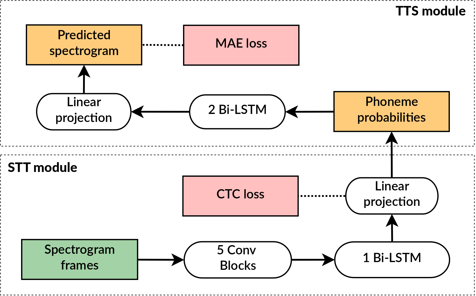
Figure 1: Forced-aligner autoencoder architecture overview.

To extract phoneme durations, we discard the decoder (TTS) module and use the speech-to-text encoder to calculate phoneme posteriors. Then, we use Dijkstra’s algorithm to find the most likely monotonic path through the sequence of phoneme probabilities.

4 Acoustic model

Recently, autoregressive neural TTS models have shown state-of-the-art performance in terms of enhanced speech naturalness [3, 14]. Despite the high synthesis quality of these models, they generally show a lack of robustness at inference time, particularly when the attention mechanism does not constrain the alignments to be monotonic. Attention failures cause mispronounciation, skipping or repeating words, and even totally unintelligible speech when the attention mechanism collapses.

To overcome such limitations, non-autoregressive parallel TTS models with explicit duration modeling have been proposed [13, 12] with similar success. These models do not only solve the undesired attention failures, but are also significantly faster than their autoregressive counterparts.

The proposed model was initially based on ForwardTacotron, an open-source non-autoregressive variant of Tacotron [1] inspired on parallel TTS models like FastSpeech [5] or DurIAN [6]. The original architecture was composed of two PreNet bottleneck layers, a CBHG encoder [1], a variance duration predictor similar to  [5], a 2-layer Bi-LSTM decoder and a convolutional residual PostNet as in [3]. However, following more recent works, we have introduced several modifications to this original architecture. The final modified architecture is depicted in Figure 2, and the introduced modifications are described in detail next.

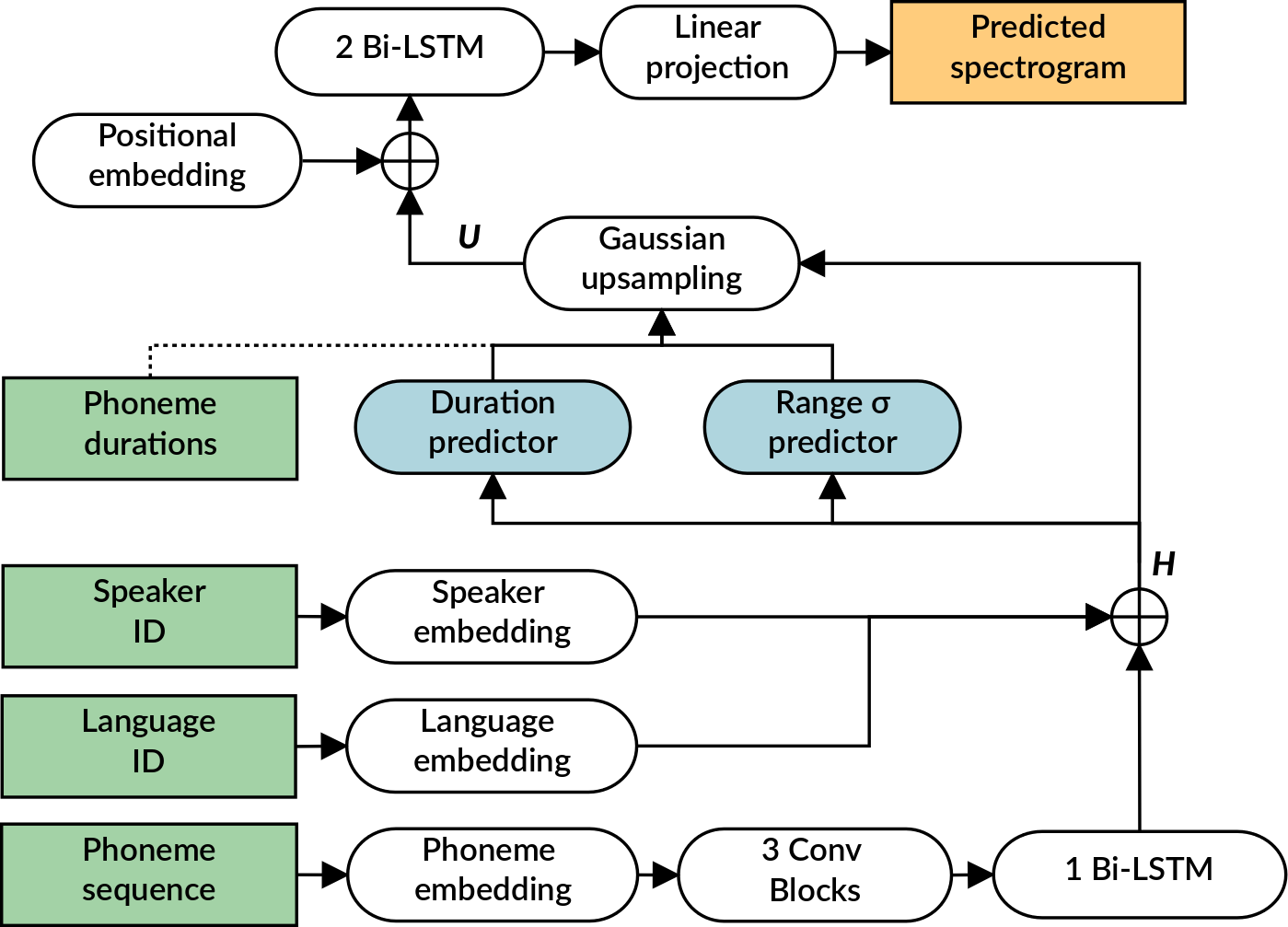
Figure 2: Proposed TTS acoustic model architecture. Dashed lines are training-only connections.

First, we replaced the encoder module with the simplified architecture proposed in Tacotron-2 [3] shown at the bottom of Figure 2. The encoder module consists of learned 512-dimensional phoneme embeddings that are passed through a stack of three 1-D convolutional layers, followed by batch normalization and ReLU activations. The output of the last convolutional layer is processed by a single bidirectional LSTM layer to generate the encoder hidden states. These states are later expanded attending to phoneme durations and consumed by a decoder to generate the spectrogram frames.

Second, we replaced the vanilla upsampling through repetition (also known as length regulator module) in favor of the Gaussian upsampling approach recently proposed in [13], which has been shown to improve speech naturalness. After the upsampling, we also add Transformer-style sinusoidal positional embeddings of a frame position with respect to the current phoneme as in [19]. We also discarded the recurrent layer of the variance predictor module as we empirically found improved robustness on phoneme duration predictions, in line with [5].

Finally, we discarded the convolutional residual PostNet as we found it not to bring any noticeable improvements on the spectrogram reconstruction task when using a bi-directional LSTM decoder.

The text-to-spectrogram models are trained using a combination of the $\mathcal{L}1$ loss and the structural similarity index measure (SSIM) between the predicted and the target spectrograms, and Hubber loss for logarithmic duration prediction [20].

5 Vocoder model

The public HiFi-GAN implementation is used for reconstructing the audio waveform conditioned on the generated spectrograms. We choose the HiFi-GAN V1 ($h_{u}=512$), which is the larger HiFi-GAN model proposed in the original paper and brings the better audio quality compared to the reduced V2 and V3 models [11]. It was trained only on the audio recordings provided by the organization. The training procedure comprises two steps. Initially, the vocoder model is trained on the extracted ground-truth spectrograms for 500K steps. Then, after the acoustic model is trained, ground-truth aligned (GTA) spectrograms are generated for the training dataset and the HiFi-GAN model is fine-tuned on the acoustic model outputs for an additional 100K steps, which helps reducing the artifacts induced by the missmatch between the vocoder training and inference conditions and brings slightly better audio quality for the TTS task.

6 Subjective results

A total of 12 participating teams submitted their generated test samples to be evaluated in the subjective listening test. Table 2 describes the different aspects considered for the subjective evaluation test. Our system was assigned the letter J, while R corresponds to the original audio recordings.

Table 2: Subjective evaluation sections

Section	Aspect	Metric
Sections 1 and 2	Speaker similarity	MOS (1-5)
Sections 3 and 4	Naturalness	MOS (1-5)
Section 5 (Sharvard)	Intelligibility	WER %
Section 6 (SUS)	Intelligibility	WER %

The listeners participating in the subjective test could be divided into three different groups:

• SP: Paid participants (native speakers of Spanish)

• SE: Volunteer speech experts (self-identified as such)

• SR: Rest of volunteers

6.1 Naturalness

In the speech naturalness test (sections 3 and 4), listeners listened to one sample and chose a score which represented how natural or unnatural the sentence sounded on a scale of 1 (completely unnatural) to 5 (completely natural). Building systems that can achieve a high degree of naturalness is probably the most challenging task when it comes to generate synthetic speech, and thus the speech naturalness MOS has become the main metric to evaluate speech synthesis quality over the last few years.

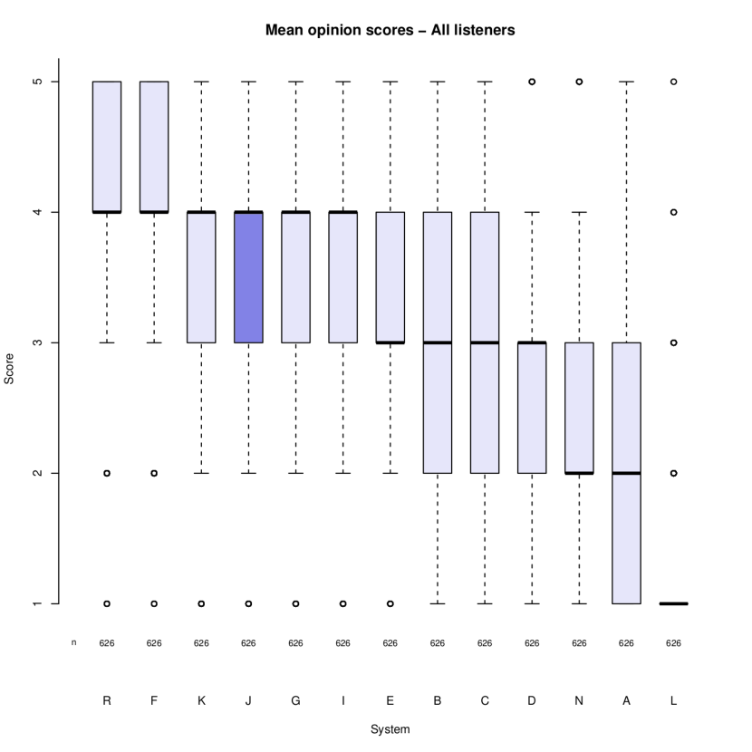
Figure 3: Naturalness MOS for all participants (all listeners)

The boxplot evaluation results of all systems on speech naturalness from all listeners is showed in Figure 3. In this case, system F performed clearly better than other systems. Our system was scored with a naturalness MOS of $3.61$ in terms of speech naturalness, while the real recordings were scored with $4.21$. As can bee seen in Figure 3, our system performance is comparable to that of systems K, G and I, all of them ranked in a second position just after system F. We believe this result is very positive, especially when considering our system was trained with a limited amount of data ($\sim$5 hours) to what is common in two-stage neural TTS pipelines (20 hours or more) [21, 22].

6.2 Speaker similarity

In the speaker similarity test (sections 1 and 2), listeners could play 2 reference samples of the original speaker and one synthetic sample. They chose a response that represented how similar the synthetic voice sounded to the voice in the reference samples on a scale from 1 (sounds like a totally different person) to 5 (sounds like exactly the same person).

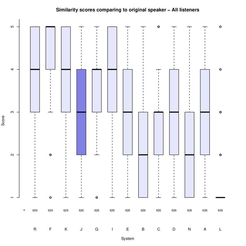
Figure 4: Speaker similarity scores for all participants (all listeners)

The boxplot evaluation results of all systems on speaker similarity from all listeners is showed in Figure 4. System F, K and I performed better than other systems. Despite the fact that our system (J) was only trained with the data provided by the Blizzard Challenge 2021 organizers, it was scored with a speaker similarity MOS of $3.29$ compared to $4.07$ from the original recordings (R).

6.3 Intelligibility test

Finally, an intelligibility test was carried out in sections 5 and 6. The goal of this test was just to determine whether or not the synthetic speech was understandable. Listeners heard one utterance in each part and typed in what they heard. Listeners were allowed to listen to each sentence only once. The sentences were specially designed to test the intelligibility of the synthetic speech: the sentences and the reference natural recordings for section 5 came from the Sharvard corpus, while the SUS for section 6 were kindly provided by TALP-UPC and Aholab-EHU research laboratories.

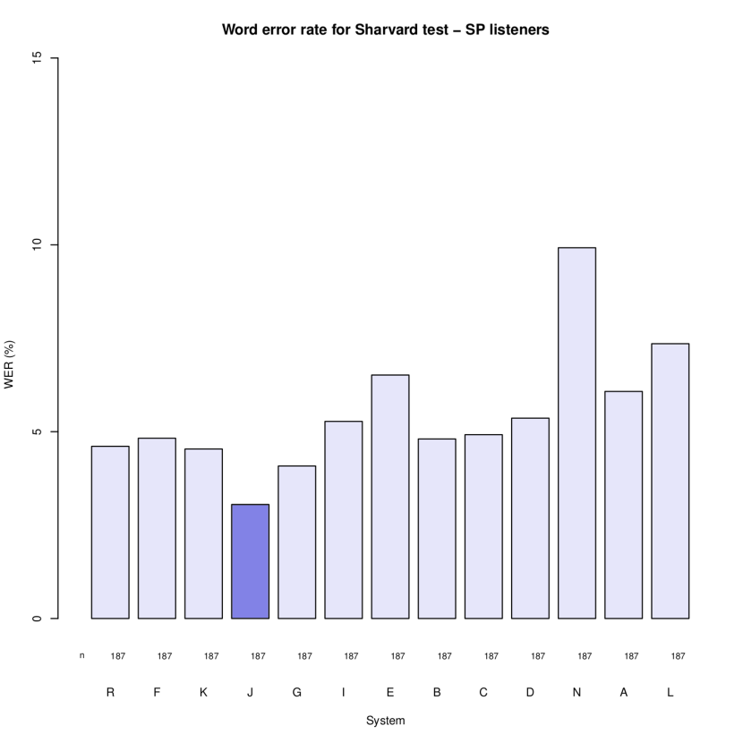
Figure 5: Intelligibility Word Error Rates (WER) for the Sharvard intelligibility test

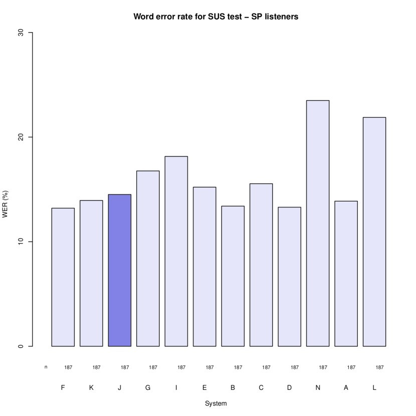
Figure 6: Intelligibility Word Error Rates (WER) for the SUS intelligibility test

Figure 5 shows the Word Error Rates (WER) of all teams for the Sharvard intelligibility test, where our system achieved the lowest transcription error ($3.0$%). This result emphasizes the good performance of our model regarding word pronunciation even though it was trained with a limited amount of speech data. Figure 6 shows the WER for the SUS intelligibility test, where our system performs similarly to the best performing systems.

7 Conclusions

In this work we have presented our proposed two-stage neural text-to-speech system for the Blizzard Challenge 2021. Both the acoustic and the vocoder models were trained using only the data provided by the organization (close to 5 hours of studio-quality recordings from a Spanish female native speaker). In the subjective listening tests, our system (identified as J) performance in terms of speech naturalness MOS was ranked in second position along with 3 other systems.

8 Acknowledgements

The research leading to these results has received funding from the Government of Spain’s research project Multisub (ref. RTI2018-094879-B-I00, MCIU/AEI/FEDER,EU).

References

- [1] Y. Wang et al., “Tacotron: Towards end-to-end speech synthesis,” in Proc. of Interspeech, 2017, pp. 4006–4010.
- [2] S. Ö. Arik, M. Chrzanowski, A. Coates, G. Diamos, A. Gibiansky, Y. Kang, X. Li, J. Miller, A. Ng, J. Raiman, S. Sengupta, and M. Shoeybi, “Deep voice: Real-time neural text-to-speech,” in ICML, 2017.
- [3] J. Shen et al., “Natural TTS Synthesis by Conditioning Wavenet on MEL Spectrogram Predictions,” in Proc. of ICASSP, 2018, pp. 4779–4783.
- [4] N. Li, S. Liu, Y. Liu, S. Zhao, M. Liu, and M. Zhou, “Close to human quality tts with transformer,” ArXiv, vol. abs/1809.08895, 2018.
- [5] Y. Ren et al., “FastSpeech: Fast, Robust and Controllable Text to Speech,” in Proc. of NIPS, 2019.
- [6] C. Yu et al., “Durian: Duration informed attention network for speech synthesis,” Proc. of Interspeech, pp. 2027–2031, 2020.
- [7] Y. Ren, C. Hu, X. Tan, T. Qin, S. Zhao, Z. Zhao, and T.-Y. Liu, “Fastspeech 2: Fast and high-quality end-to-end text to speech,” in International Conference on Learning Representations, 2021. [Online]. Available: https://openreview.net/forum?id=piLPYqxtWuA
- [8] A. Hunt and A. Black, “Unit selection in a concatenative speech synthesis system using a large speech database,” in 1996 IEEE International Conference on Acoustics, Speech, and Signal Processing Conference Proceedings, vol. 1, 1996, pp. 373–376 vol. 1.
- [9] A. W. Black and P. A. Taylor, “Automatically clustering similar units for unit selection in speech synthesis.” 1997.
- [10] H. Zen, K. Tokuda, and A. W. Black, “Statistical parametric speech synthesis,” Speech Communication, vol. 51, no. 11, pp. 1039–1064, 2009. [Online]. Available: https://www.sciencedirect.com/science/article/pii/S0167639309000648
- [11] J. Su, Z. Jin, and A. Finkelstein, “Hifi-gan: High-fidelity denoising and dereverberation based on speech deep features in adversarial networks,” in INTERSPEECH, 2020.
- [12] A. Łańcucki, “Fastpitch: Parallel text-to-speech with pitch prediction,” 2020.
- [13] J. Shen et al., “Non-Attentive Tacotron: Robust and Controllable Neural TTS Synthesis Including Unsupervised Duration Modeling,” arXiv preprint arXiv:2010.04301, 2020.
- [14] N. Li, S. Liu, Y. Liu, S. Zhao, and M. Liu, “Neural speech synthesis with transformer network,” in Proceedings of the AAAI Conference on Artificial Intelligence, vol. 33, no. 01, 2019, pp. 6706–6713.
- [15] M. McAuliffe, M. Socolof, S. Mihuc, M. Wagner, and M. Sonderegger, “Montreal forced aligner: Trainable text-speech alignment using kaldi.” in Interspeech, vol. 2017, 2017, pp. 498–502.
- [16] M. He et al., “Robust Sequence-to-Sequence Acoustic Modeling with Stepwise Monotonic Attention for Neural TTS,” in Proc. of Interspeech, 2019, pp. 1293–1297.
- [17] E. Battenberg et al., “Location-Relative Attention Mechanisms for Robust Long-Form Speech Synthesis,” in Proc. of ICASSP, 2020, pp. 6194–6198.
- [18] A. Graves et al., “Connectionist temporal classification: labelling unsegmented sequence data with recurrent neural networks,” in Proc. of ICML, 2006, pp. 369–376.
- [19] I. Elias et al., “Parallel Tacotron: Non-Autoregressive and Controllable TTS,” arXiv preprint arXiv:2010.11439, 2020.
- [20] J. Vainer and O. Dušek, “SpeedySpeech: Efficient Neural Speech Synthesis,” in Proc. of Interspeech, 2020, pp. 3575–3579.
- [21] K. Ito and L. Johnson, “The lj speech dataset,” https://keithito.com/LJ-Speech-Dataset/, 2017.
- [22] C. Veaux, J. Yamagishi, and K. MacDonald, “Cstr vctk corpus: English multi-speaker corpus for cstr voice cloning toolkit,” 2017.