Convergence of Uncertainty Sampling for Active Learning

Abstract

Uncertainty sampling in active learning is heavily used in practice to reduce the annotation cost. However, there has been no wide consensus on the function to be used for uncertainty estimation in binary classification tasks and convergence guarantees of the corresponding active learning algorithms are not well understood. The situation is even more challenging for multi-category classification. In this work, we propose an efficient uncertainty estimator for binary classification which we also extend to multiple classes, and provide a non-asymptotic rate of convergence for our uncertainty sampling based active learning algorithm in both cases under no-noise conditions (i.e., linearly separable data). We also extend our analysis to the noisy case and provide theoretical guarantees for our algorithm under the influence of noise in the task of binary and multi-class classification.

1 Introduction

Over the last decade, machine learning algorithms have achieved a lot of success on various tasks in computer vision, natural language processing, and speech recognition. This success has been led by various factors which include improvement in computing architectures and improved machine learning algorithms. Moreover, the rapid growth in the number of large labeled public datasets is also one of the most important factors which contributed to the rise of machine learning. However, in many practical scenarios, the labeled data are hard to obtain, as it requires a lot of time and human efforts to label a dataset. Hence, it is a time consuming as well as economically expensive procedure to perform. For this reason, there have been a lot of efforts to build machine learning algorithms which require a significantly lower number of labeled samples to train. One major direction of research in this area is to devise efficient active learning algorithms.

Active learning algorithms propose efficient labeling schemes to reduce the number of labels required in order to train a classifier, resulting in minimal annotation cost while still maintaining high performance. Active learning methods can be categorized in two major categories : (i) stream-based active learning where samples from the data generating distribution are sequentially presented to the active learner, and (ii) pool-based active learning where there exists a very small number of labeled samples and the rest of the samples have no label. We note that any streaming based active learning algorithm can be converted to a pool-based active learning algorithm and vice versa [20]. For both of these categories, there exists an acquisition function which characterizes which informative samples should be labelled. The most popular way of determining if a sample is informative or not is by estimating uncertainty. Other than uncertainty sampling based approaches, the other major approaches for performing active learning are query-by-committee [24], expected model change [23], expected error reduction [19], expected variance reduction [29], among others.

The main focus of this paper is uncertainty sampling based active learning algorithms. Despite of it being one of the most used active learning algorithms in practice, little is known about its theoretical properties. Specifically, there has been no common consensus on the optimal uncertainty estimation approach used to perform active learning and its convergence properties. Also, most of the active learning algorithms studied previously are for binary classification and are not trivial to extend to multi-category classification problems. In this paper, we investigate these questions from the lens of optimization through stochastic gradient descent, and propose a sampling function for which the uncertainty sampling based active learning algorithm provably converges. We make the following contributions in this work :

• We propose a family of theoretically motivated functions to estimate uncertainty for linear predictions for binary and multi-category classification.

• We show that the active learning algorithm based on the proposed sampling scheme converges to the optimal predictor in the separable regime for binary classification, and can be easily extended to multi-category classification. We provide a non-asymptotic rate of convergence of order ${O}(1/n)$, where $n$ is number of iterations of the algorithms which is also number of unlabeled samples seen by the algorithm for both binary and multi-class cases.

• We extend our analysis to the inseparable regime for both cases (binary and multi-class) and show that the probability of mis-classification is bounded by ${O}(1/n)+{O}(\eta)$ where $n$ is number of iteration performed by the algorithms and $\eta$ is the noise parameter.

• We perform experimental evaluations for our algorithm on classification tasks.

1.1 Related Work

There has been a vast amount of work done in the field of active learning and we only give a brief overview here. For binary classification, online active learning has been studied under the name of selective sampling under adversarial assumptions [5, 8, 17, 4]. However, these methods can not be extended to multi-class classification and are computationally expensive. Agarwal [1] proposed a selective sampling scheme for multi-class classification for generalized linear models, but still each step of the algorithm is computationally expensive to perform. Settles [22] provides an excellent survey of empirical studies in active learning.

Apart from empirical studies, there has been a lot of works in active learning on the theoretical front. Disagreement based active learning has been an active area of research in machine learning. The primary idea is as follows. A set of possible empirical risk minimizers are maintained with time and a label is queried if two minimizers disagree on the predicted label of that sample. An excellent survey of disagreement based active learning is provided in [9].

Our work can also be related to the vast line of work done in margin based active learning [3, 7, 2, 30]. However for most of works in this area, the gain and convergence of the algorithm have only been shown under strong distributional assumptions while we do not make any such assumption on the data for our uncertainty sampling based active learning algorithm, and still manage to show a non-asymptotic rate of convergence for the algorithm.

Uncertainty sampling based machine learning algorithms have a long history. They were first proposed by Lewis and Gale [11] who experimentally show that a probabilistic model with uncertainty sampling can improve the performance of text classification by up to 500 fold. Later, Schohn and Cohn [21] applied uncertainty sampling to SVM classification and showed improved performance. Since then, it has been widely used for performing active learning [32, 33, 12, 31, 28]. However, none of the above mentioned works focuses on the theoretical understanding of uncertainty sampling. Recently, Mussmann and Liang [15] showed that threshold based uncertainty sampling on a convex (e.g., logistic) loss can be interpreted as performing a preconditioned stochastic gradient step on the population zero-one loss. However, a proper convergence analysis was missing in [15], in part due to the underlying non-convexity of their formulation.

2 Background

2.1 Uncertainty Sampling

Because of the ease of application, uncertainty sampling remains one of the most popular approaches used to perform active learning. Uncertainty sampling relies on the idea of querying the data point about which the current predictor is most uncertain. In simpler terms, uncertainty sampling usually identifies those points which are close to the decision boundary of the current model. However, the most important task here is to compute the uncertainty of prediction. There have been several approaches proposed to measure the uncertainty of a prediction. Here below, we discuss few of them that are widely used in practice [14]. Let us assume that a probabilistic model generates predictions in the form of probability distributions $p_{\theta}(\cdot|x)$ on $\mathcal{Y}$ for $x\in\mathcal{X}$ and model parameter $\theta$.

Margin of confidence sampling [14, 16]. An intuitive way to estimate the uncertainty is by computing the margin in the confidence of top two predictions. Mathematically, sampling probability of querying a label $p_{u}(x,\theta)=\sigma(p_{\theta}(y_{1}^{\star}|x)-p_{\theta}(y_{2}^{\star}|x))$ where $\sigma:\mathbb{R}\rightarrow[0,1]$, and $y_{1}^{\star}$ and $y_{2}^{\star}$ correspond to the two top most predictions for $x$ given the model parameter $\theta$.

Least confidence sampling [14, 16]. Least confidence sampling considers the difference between 100% confidence and the most confident prediction to compute sampling probability of query a label. That means $p_{u}(x,\theta)\propto 1-p_{\theta}(y_{1}^{\star}|x)$ where $y_{1}^{\star}$ corresponds to the top most prediction for $x$ given the model parameter $\theta$.

Entropy-based sampling [14, 16]. Entropy is an information theoretically motivated way to compute the uncertainty and widely used to estimate the uncertainty. Sampling probability of querying a label can be written as: $p_{u}(x,\theta)\propto\sum_{y\in\mathcal{Y}}p_{\theta}(y|x)\log p_{\theta}(y|x)$.

In this paper, we use the margin of confidence sampling scheme to estimate uncertainty in the prediction. Details of the sampling function $\sigma$ will be provided in section 3 where we discuss convergence of the algorithm. However, before discussing the theoretical results (section 3), in the next section we discuss the relation between the hinge loss and corresponding test accuracy in binary and multi-class classification.

2.2 Max-margin linear classification

In this paper, we consider the simplest possible set-up of linear classification, with inputs $x\in\mathbb{R}^{d}$, and linear prediction functions. We note that by replacing $x$ by some feature function $\Phi(x)$ we can deal with non-linear problems, the feature map being explicit or implicit through kernel methods [10].

Binary classification. With two classes, we consider $y\in\{-1,1\}$ and a prediction function $x\mapsto\theta^{\top}x$ parameterized by $\theta\in\mathbb{R}^{d}$. We then classify according to the sign of $\theta^{\top}x$.

The associated error rate can be computed as

$${\mathbb{P}}(y\theta^{\top}x\leqslant 0),$$

but is is a non-convex function of $\theta$. Among the many convex surrogates, we will consider the classical hinge loss:

$$\hat{\ell}(x,y,\theta)=\max\{0,1-y\theta^{\top}x\},$$

and its square, leading to the traditional support vector machine. The regular hinge loss is non differentiable, while the squared hinge loss is smooth in $\theta$. In this paper, we will consider an algorithm based on the squared hinge loss, but obtain a guarantee for the non-squared one. Given that the two losses lead to guarantees on the misclassification error, as

$${\mathbb{P}}(y\theta^{\top}x\leqslant 0)\leqslant{\mathbb{E}}(\hat{\ell}(x,y,\theta))$$

$${\mathbb{P}}(y\theta^{\top}x\leqslant 0)\leqslant{\mathbb{E}}(\hat{\ell}(x,y,\theta)^{2}),$$

this allows to get the desired bounds.

Multi-class classification. Here, we consider $y\in\{1,\dots,k\}$. In multi-class classification the model parameter $\theta$ is a vector in $\mathbb{R}^{dk}$ which consists of predictors $\theta(i)\in\mathbb{R}^{d}$ for all $i\in\{1,2,\ldots,k\}$. Hence, we denote model parameter $\theta$ as collection of $k$ predictors, i.e., $\theta=[\theta(1);\theta(2);\cdots;\theta(k)]$. We consider the multi-class SVM formulation of [6]. Following the structured SVM notation in [25], let us assume that $\phi(x,y)$ represents the feature map corresponding to the sample pair $(x,y)$. In multi-class classification with $k$ classes, $\phi(x,y)\in\mathbb{R}^{dk}$ consists of $k$ blocks of $d$-dimensional vector and if we allow ourselves to denote each $d$-dimensional block with $\phi(x,y)(i)$ for $i\in\{1,2,\cdots,k\}$, then $\phi(x,y)=[\phi(x,y)(1);\phi(x,y)(2);\cdots;\phi(x,y)(k)]$ where $\phi(x,y)(i)=0$ for all $i\neq y$ and $\phi(x,y)(y)=x$. Define a loss function $\Delta:\mathcal{Y}\times\mathcal{Y}\rightarrow\mathbb{R}$. General hinge loss for maximum margin training function can be written as :

$$\hat{\ell}(x_{t},y_{t},\theta)=\max_{y\in\mathcal{Y}}\left[\Delta(y,y_{n})-\theta^{\top}(\phi(x_{n},y_{n})-\phi(x_{n},y))\right].$$

In the case of multi-class classification, generally $\Delta(y,y^{\prime})=1$ if $y\neq y^{\prime}$, otherwise $\Delta(y,y^{\prime})=0$. Hence, the multi-class hinge loss can be written as,

$$\hat{\ell}(x,y,\theta)=\max\left[0,1-\theta^{\top}\left(\phi(x,y)-\phi(x,y^{\star}(\theta,x,y)\right)\right],$$ (1)

$$\text{where}~{}~{}y^{\star}(\theta,x,y)=\mathop{\rm arg\,max}_{z\in{\mathcal{Y}\backslash{y}}}\theta^{\top}\phi(x,z).$$

Predicting a label for the data point $x\in\mathbb{R}^{d}$ by the predictor $\theta$ is done by computing $\mathop{\rm arg\,max}_{z\in{\mathcal{Y}}}\theta^{\top}\phi(x,z)$. Similar to the binary case, the hinge loss for multiclass classification is non differentiable while the square hinge loss is smooth and differentible in model parameter $\theta$. For multi-class hinge loss as well, the misclassification error can be bounded by expected loss for both the losses. That is for a given sample pair $(x,y)$ and model parameter $\theta$, we have,

$${\mathbb{P}}(\theta^{\top}\phi(x,y)-\theta^{\top}\phi(x,z^{\star})\leqslant 0)\leqslant{\mathbb{E}}(\hat{\ell}(x,y,\theta))$$

$${\mathbb{P}}(\theta^{\top}\phi(x,y)-\theta^{\top}\phi(x,z^{\star})\leqslant 0)\leqslant{\mathbb{E}}(\hat{\ell}(x,y,\theta)^{2}),$$

where $z^{\star}=\mathop{\rm arg\,max}_{z\in{\mathcal{Y}}}\theta^{\top}\phi(x,z)$.

3 Convergent Uncertainty Sampling for Classification

1

Input: learning rate $\gamma$, Streaming $(x_{i},y_{i})$ for $i\in[n]$, initial model parameter $\theta_{1}$, parameter $\mu$ and sampling function $\sigma$.

;

Output: average iterate $\bar{\theta}_{n+1}$.

for $t\leftarrow 1$ to $n$  do

         Compute probability $p_{u}(x_{t},\theta_{t})=\sigma(\theta_{t},x_{t}).$

       Sample Bernoulli random variable $z_{t}$ with $p=p_{u}(x_{t},\theta_{t}).$

       Compute $\hat{\ell}_{t}(x_{t},y_{t},\theta_{t})\leftarrow\max(0,1-y_{t}(\theta_{t}^{\top}x_{t})).$

       Update $\theta_{t+1}\leftarrow\theta_{t}+\gamma z_{t}(y_{t}x_{t})\hat{\ell}_{t}(x_{t},y_{t},\theta_{t}).$

       Update $\bar{\theta}_{t+1}\leftarrow\left(1-\frac{1}{t+1}\right)\bar{\theta}_{t+1}+\frac{1}{t+1}\theta_{t+1}.$

Algorithm 1 Uncertainty Sampling in Binary Classification

In this work, we consider the streaming data setting. However, the algorithm can also be applied for non-streaming data setting. In the next three sections, we would discuss the convergence results for binary and multi-class classification.

Let us consider $n$ i.i.d. samples $(x_{i},y_{i})$ jointly sampled from $\mathcal{P}$ such that $x_{i}\in\mathbb{R}^{d}$, $i=1,\dots,n$, and $y_{i}\in\mathcal{Y}$ where $\mathcal{Y}=\{-1,1\}$ for binary classification and $\mathcal{Y}=\{1,2,\ldots,k\}$ for multi-class classification.

Before going into the details of theoretical results, we discuss the intuition of the uncertainty sampling algorithm here below. As discussed previously, the main idea behind the uncertainty sampling based active learning algorithm is that to query the labels for those data point about which the predictor is uncertain about. In streaming data setting, every-time we see a new data point, we compute its uncertainty by computing the prediction score. Then, we convert this score into the density function with the help of the given function $\sigma$ which maps prediction score to probability of querying a label. This probability score is used to generate a Bernoulli random variable which decides if the algorithm would query the label of the presented sample or not, and then perform a stochastic gradient step (for the squared hinge loss) if the label is accessed. The exact expression for the function $\sigma$ would be provided in section 3.1 (for binary classification) and in section 3.2 for multiclass classification. The pseudo-codes of the algorithms are presented in algorithm 1 (binary classification) and algorithm 2 (multi-class classification).

1

Input: learning rate $\gamma$, Streaming $(x_{i},y_{i})$ for $i\in[n]$, initial model parameter $\theta_{1}$, parameter $\mu$, number of classes k, and sampling function $\sigma$.

Output: average iterate $\bar{\theta}_{n+1}$.

for $t\leftarrow 1$ to $n$  do

         Compute score $s_{t}(j)=\theta(j)^{\top}x_{t}$ for all $j\in[k]$ .

       Compute probability $p_{u}(x_{t},\theta_{t})=\sigma(\theta_{t},x_{t}).$

       Sample Bernoulli random variable $z_{t}$ with $p=p_{u}(x_{t},\theta_{t}).$

       $y_{t}^{\star}\leftarrow\mathop{\rm arg\,max}_{j\in\mathcal{Y}\backslash y_{t}}s_{t}(j)$

       $\hat{\ell}_{t}(x_{t},y_{t},\theta_{t})\leftarrow\max(0,1-\theta_{t}(y_{t})^{\top}x_{t}+\theta_{t}(y_{t}^{\star})^{\top}x_{t}).$

       Update $\theta_{t+1}(y_{t})\leftarrow\theta_{t}(y_{t})+\gamma z_{t}x_{t}\hat{\ell}_{t}(x_{t},y_{t},\theta_{t}).$

       Update $\theta_{t+1}(y_{t}^{\star})\leftarrow\theta_{t}(y_{t}^{\star})-\gamma z_{t}x_{t}\hat{\ell}_{t}(x_{t},y_{t},\theta_{t}).$

       Update $\theta_{t+1}\leftarrow[\theta_{t+1}(1);\theta_{t+1}(2);\ldots;\theta_{t+1}(k)].$

       Update $\bar{\theta}_{t+1}\leftarrow\left(1-\frac{1}{t+1}\right)\bar{\theta}_{t+1}+\frac{1}{t+1}\theta_{t+1}.$

Algorithm 2 Uncertainty Sampling in Multi-Class Classification

3.1 Binary Classification

In the separable case for binary classification we, assume that there exists an optimal classifier $\theta_{\star}\in\mathbb{R}^{d}$ such that for all $x\in\mathcal{X}$ and its corresponding label $y\in\mathcal{Y}$ where $\mathcal{Y}=\{-1,1\}$,

$$y(\theta_{\star}^{\top}x)\geq\rho^{\star}>1.$$ (2)

The above assumption is a standard assumption made in the analysis of maximum margin classifier in the realizable case [3, 7]. We minimize the square hinge loss to obtain our predictor. The expression for square hinge loss can be written as (with an extra factor of $1/2)$,

$$\ell(x,y,\theta)=\frac{1}{2}\max\left[0,1-y\theta^{\top}x\right]^{2}.$$ (3)

We have the following update rule to update the model parameter $\theta$ for uncertainty sampling based active learning :

$$\theta_{t+1}=\theta_{t}+\gamma~{}z_{t}(y_{t}x_{t})\big{[}1-y_{t}({\theta_{t}}^{\top}x_{t})\big{]}_{+},$$ (4)

where $z_{t}$ is a Bernoulli random variable for fixed $\theta_{t}$ and $x_{t}$ such that $p(z_{t}=1|x_{t},\theta_{t})=\sigma(\theta_{t},x_{t})$ where $\sigma:\mathbb{R}^{d}\times\mathbb{R}^{d}\rightarrow[0,1]$ is an even function.

When $\sigma=1$, i.e., querying label for every sample, then this is exactly stochastic gradient descent for the squared hinge loss, which is known to converge with rate $O(1/t)$ in the separable situation [27]. In the next result we show that the algorithm proposed in this paper (algorithm 1) converges.

Theorem 1.

Consider a set of $n$ i.i.d samples $(x_{i},y_{i})$ jointly sampled from $\mathcal{P}$ such that $x_{i}\in\mathbb{R}^{d}$, and $y_{i}\in\{-1,1\}$ for all $i=1,\dots,n$ then under the assumption that there exists a $\theta_{\star}$ for which $y(\theta_{\star}^{\top}x)\geq\rho^{\star}$ for all $(x,y)$ pair in $\mathcal{P}$, the following convergence guarantee exists for Algorithm 1,

$${\mathbb{E}}(1-y\theta_{t}^{\top}x)_{+}\leq\frac{R^{2}\max\left\{1,\frac{1}{\mu}\right\}\|\theta_{1}-\theta_{\star}\|^{2}}{\min\left\{\frac{1}{\mu},\frac{\rho^{\star}-1}{1+\mu}\right\}^{2}n},$$ (5)

for the choice of $\sigma(\theta,x)=\frac{1}{1+\mu|\theta^{\top}x|}$, step size $\gamma=\frac{\min\left\{\frac{1}{\mu},\frac{\rho^{\star}-1}{1+\mu}\right\}}{R^{2}\max\left\{1,\frac{1}{\mu}\right\}}$ and $\|x\|\leq R$ for all $x$ in the domain $\mathcal{X}$.

Proof sketch.

See the complete proof given in the Appendix. Using the update given in eq. 4 and taking expectations only with respect to $z_{t}$ considering $x_{t},y_{t},\theta_{t}$ fixed, we get the following

$${\mathbb{E}}\left\|\theta_{t+1}-\theta_{\star}\right\|^{2} =\left\|\theta_{t}-\theta_{\star}\right\|^{2}+2\gamma\sigma(\theta_{t},x_{t})\big{[}1-y_{t}({\theta_{t}}^{\top}x_{t})y_{t}(\theta_{t}^{\top}x_{t}-y_{t}{\theta_{\star}}^{\top}x_{t})\big{]}_{+}$$

$$\qquad\qquad\qquad\qquad\qquad\qquad+\gamma^{2}\sigma(\theta_{t},x_{t})R^{2}\big{[}1-y_{t}({\theta_{t}}^{\top}x_{t})\big{]}_{+}^{2},$$

where $R$ is the upper bound on $\|x\|$ for all $x\in\mathcal{X}$. Our next goal is to find the function $\sigma(\theta,x)$ which satisfy the following properties for $y_{t}\theta_{t}^{\top}x_{t}<1$,

$$\sigma(\theta_{t},x_{t})(1-y_{t}\theta_{t}^{\top}x_{t})_{+}^{2}\leq c_{1}(1-y_{t}\theta_{t}^{\top}x_{t})_{+}$$ (6)

$$\sigma(\theta_{t},x_{t})(y_{t}\theta_{t}^{\top}x_{t}-y_{t}{\theta_{\star}}^{\top}x_{t})\leq-c_{2},$$ (7)

for some positive constants $c_{1}$ and $c_{2}$. We show in Lemma 1 that choosing

$$\sigma(\theta,x)=\frac{1}{1+\mu|\theta^{\top}x|},$$ (8)

for $\mu>0$ satisfies the conditions in eq. 6 and eq. 7 for $c_{1}\geq\max\left\{1,\frac{1}{\mu}\right\}$ and $c_{2}\leq\min\left\{\frac{\rho^{\star}-1}{1+\mu},\frac{1}{\mu}\right\}$. Finally, after taking expectations, applying Jensen’s inequality, and for the optimal choice of step size $\gamma$, we get

$${\mathbb{E}}(1-y\theta_{t}^{\top}x)_{+}\leq\frac{R^{2}\max\left\{1,\frac{1}{\mu}\right\}\|\theta_{1}-\theta_{\star}\|^{2}}{\min\left\{\frac{1}{\mu},\frac{\rho^{\star}-1}{1+\mu}\right\}^{2}n}.$$

∎

On Mistake Bound.

As discussed in section 2.2, the probability of misclassification is bounded by the expected classification loss (non squared hinge loss). Hence, for an independently sampled pair $(x,y)$,

$${\mathbb{P}}(y\bar{\theta}_{n}^{\top}x\leq 0)\leq\frac{R^{2}\max\left\{1,\frac{1}{\mu}\right\}\|\theta_{1}-\theta_{\star}\|^{2}}{\min\left\{\frac{1}{\mu},\frac{\rho^{\star}-1}{1+\mu}\right\}^{2}n}.$$ (9)

Discussion.

It is important to note that the conditions mentioned in eq. 6 and eq. 7 are required only when $y_{t}\theta_{t}x_{t}<1$ as the gradient is zero when $y_{t}\theta_{t}x_{t}\geq 1$, and hence the model parameter is not updated. Ideally, the label should not be queried when $y_{t}\theta_{t}x_{t}\geq 1$, however there is no way to compute it beforehand. Hence, our sampling scheme provides a good trade-off for sampling. The value of $\mu$ should be decided by experimental evaluation as for $\mu\rightarrow\infty$, the upper bound for our algorithm seems to diverge.

Denoting the expected number of samples labelled in $t$ steps as $\#_{t}$, we get:

$$\#_{n} =\sum_{t=0}^{n-1}\sigma(\theta_{t},x_{t})=\sum_{t=0}^{n-1}\frac{1}{1+\mu|\theta_{t}^{\top}x_{t}|},$$

which can be significantly less than $n$ if the absolute value of $\theta_{t}^{\top}x_{t}$ is large for most of $t$, i.e., most of the points are far from the decision boundary.

3.2 Extension to Multi-class Classification

In the separable multi-class case, we assume that there exists a set of optimal half-spaces $\theta_{\star}(i)\in\mathbb{R}^{d}$ for $i\in\{1,2,\ldots,k\}$ corresponding to each class such that for all $x\in\mathcal{X}$ and its corresponding label $y\in\mathcal{Y}$ where $\mathcal{Y}=\{1,2,\ldots,k\}$,

$$(\theta_{\star}(i)-\theta_{\star}(j))^{\top}x\geq\rho^{\star}>1~{}\text{for all }i\neq j\in[k].$$ (10)

Note that the loss function given in eq. 1 is the same as that of used to compute the loss in algorithm 2. We will optimize the multi-class square hinge loss and not the hinge loss for the reason discussed in section 2.2. Let us introduce the following notation,

$$\delta_{x}(y,y^{\prime})=\phi(x,y)-\phi(x,y^{\prime}).$$

Hence, the expression for the square hinge loss is

$${\ell}(x,y,\theta)=\frac{1}{2}\hat{\ell}^{2}(x,y,\theta)=\frac{1}{2}\left[1-\theta^{\top}\delta_{x}\left(y,y^{\star}(\theta,x,y)\right)\right]_{+}^{2}.$$

The gradient of $\ell(x,y,\theta)$ with respect to $\theta$ can be written as,

$$\nabla{\ell}(x,y,\theta)=-\hat{\ell}(x,y,\theta)\delta_{x}\left(y,y^{\star}(\theta,x,y)\right).$$

We consider the projected stochastic gradient descent update to to update the model parameter $\theta$ for uncertainty sampling based active learning in multi-class classification:

$$\theta_{t+1}=\Pi_{\|\theta\|\leq B}\left[\theta_{t}+\gamma z_{t}\delta_{x_{t}}\left(y_{t},y^{\star}(\theta_{t},x_{t},y_{t})\right)\hat{\ell}(x_{t},y_{t},\theta_{t})\right],$$ (11)

where $z_{t}$ is a Bernoulli random variable for fixed $\theta_{t}$ and $x_{t}$ such that $p(z_{t}=1|x_{t},\theta_{t})=\sigma(\theta_{t},x_{t})$ where $\sigma:\mathbb{R}\rightarrow[0,1]$ is an even function. $\Pi_{\|\theta\|\leq B}$ denotes the projection operator which projects $\theta_{t}$ for all $t$ in the ball of radius $B$ centered around origin. In the theorem below, we show the convergence of the algorithm proposed in algorithm 2.

Theorem 2.

Consider a set of $n$ i.i.d samples $(x_{i},y_{i})$ jointly sampled from $\mathcal{P}$ such that $x_{i}\in\mathbb{R}^{d}$, and $y_{i}\in\{1,2,\ldots,k\}$ for all $i=1,\dots,n$. Then under the assumption that there exists a set of $d$-dimensional optimal half-spaces $\theta_{\star}=\{\theta_{\star}(1),\theta_{\star}(2),\ldots,\theta_{\star}(k)\}$ corresponding to each class for which $\theta_{\star}^{\top}\delta_{x}(y,y^{\star}(\theta_{\star},x,y))\geq\rho^{\star}$ for all $(x,y)$ pair in $\mathcal{P}$, the following convergence guarantee exists for Algorithm 2 under projected gradient descent update in equation (11),

$${\mathbb{E}}\hat{\ell}(x,y,\bar{\theta}_{n})\leq\frac{R^{2}(1+BR)\|\theta_{1}-\theta_{\star}\|^{2}}{\min\left\{\frac{1}{\mu},\frac{\rho^{\star}-1}{1+\mu}\right\}^{2}n},$$ (12)

for the choice of $\sigma(\theta,x)=\frac{1}{1+\mu\left|\theta_{t}(y_{t(1)}^{\star})^{\top}x_{t}-\theta_{t}(y_{t(2)}^{\star})^{\top}x_{t}\right|}$, step size $\gamma=\min\left\{\frac{1}{\mu},\frac{\rho^{\star}-1}{1+\mu}\right\}\frac{1}{2R^{2}(1+BR)}$ and $\|\delta_{x}(i,j)\|\leq R$ for all $x$ in the domain $\mathcal{X}$, and for all $i\neq j\in[k]$ and $\|\theta\|\leq B$.

Proof sketch.

See the complete proof given in the Appendix. Using the update given in eq. 11 and taking expectations only with respect to $z_{t}$ considering $x_{t},y_{t},\theta_{t}$ fixed, we get the following

$${\mathbb{E}}\|\theta_{t+1}-\theta^{\star}\|^{2} \leq 2\gamma\sigma(\theta_{t},x_{t})\hat{\ell}(x_{t},y_{t},\theta_{t})\left(\theta_{t}^{\top}\delta_{x_{t}}\left(y_{t},y^{\star}(\theta_{t},x_{t},y_{t})\right)-{\theta^{\star}}^{\top}\delta_{x_{t}}\left(y_{t},y^{\star}(\theta_{t},x_{t},y_{t})\right)\right)$$

$$\qquad\qquad\qquad\qquad+\|\theta_{t}-\theta^{\star}\|^{2}+\gamma^{2}\sigma(\theta_{t},x_{t})R^{2}\hat{\ell}^{2}(x_{t},y_{t},\theta_{t}),$$

where $R$ is the upper bound on $\|\delta_{x}(i,j)\|$ for all $x\in\mathcal{X}$ and $i,j\in\{1,2,\dots,k\}$. Similar to the case of binary classification, we would need to find the function $\sigma(\theta,x)$ which satisfy the following properties for $\theta_{t}^{\top}\delta_{x_{t}}(y_{t},y^{\star}(\theta_{t},x_{t},y_{t}))<1$,

$$\sigma(\theta_{t},x_{t})\hat{\ell}^{2}(x_{t},y_{t},\theta_{t})\leq c_{1}\hat{\ell}(x_{t},y_{t},\theta_{t})$$ (13)

$$\sigma(\theta_{t},x_{t})\left({\theta^{\star}}^{\top}\delta_{x_{t}}\left(y_{t},y^{\star}(\theta_{t},x_{t},y_{t})\right)-\theta_{t}^{\top}\delta_{x_{t}}\left(y_{t},y^{\star}(\theta_{t},x_{t},y_{t})\right)\right)\geq c_{2},$$ (14)

for some positive constants $c_{1}$ and $c_{2}$. Let us now define top two predictions by the classifier $\theta$ for sample pair $(x,y)$ are as follows,

$$y_{(1)}^{\star}=\mathop{\rm arg\,max}_{z\in\mathcal{Y}}\theta^{\top}\phi(x,z)$$ (15)

$$y_{(2)}^{\star}=\mathop{\rm arg\,max}_{z\in\mathcal{Y}\backslash y_{(1)}^{\star}}\theta^{\top}\phi(x,z).$$ (16)

Then, we show in Lemma 2 that choosing

$$\sigma(\theta_{t},x_{t}) =\frac{1}{1+\mu\left|\theta_{t}^{\top}\delta_{x_{t}}(y_{t(1)}^{\star},y_{t(2)}^{\star})\right|}=\frac{1}{1+\mu\left|\theta_{t}(y_{t(1)}^{\star})^{\top}x_{t}-\theta_{t}(y_{t(2)}^{\star})^{\top}x_{t}\right|},$$

where $\mu$ is a positive constants, satisfies the conditions in eq. 13 and eq. 14 for $c_{1}\geq(1+BR)$ and for $c_{2}\leq\frac{\rho^{\star}-1}{1+\mu}$. Finally after taking expectations and applying Jensen’s inequality, we get the following

$${\mathbb{E}}\hat{\ell}(x,y,\bar{\theta}_{n})\leq\frac{R^{2}(1+BR)(1+\mu)^{2}\|\theta_{0}-\theta_{\star}\|^{2}}{n(\rho^{\star}-1)^{2}},$$

for all $\mu\geq 0$. ∎

On Mistake Bound.

Similar to the case of binary classification we discussed in section 2.2, the probability of misclassification for the multiclass case is bounded by the expected classification loss (multi-hinge loss). Hence, for an independently sampled pair $(x,y)$ and for $\mu\geq 0$,

$${\mathbb{P}}(\bar{\theta}_{n}^{\top}\delta_{x}(y,y^{\star}(\bar{\theta}_{n},x,y))\leq 0)\leq\frac{R^{2}(1+BR)(1+\mu)^{2}\|\theta_{0}-\theta_{\star}\|^{2}}{n(\rho^{\star}-1)^{2}}$$

$$\Rightarrow~{} {\mathbb{P}}(\bar{\theta}_{n}(y)^{\top}x-\bar{\theta}_{n}(y^{\star}(\bar{\theta}_{n},x,y))^{\top}x\leq 0)\leq\frac{R^{2}(1+BR)(1+\mu)^{2}\|\theta_{0}-\theta_{\star}\|^{2}}{n(\rho^{\star}-1)^{2}}.$$

Discussion.

It is directly not clear from the bound that how to choose $\mu$ to have a direct gain of applying active learning method. However similar to the binary classification case, the querying of a label is only required when $\theta_{t}^{\top}\delta_{x_{t}}(y_{t},y^{\star}(\theta_{t},x_{t},y_{t}))<1$ as the gradient is $0$ when $\theta_{t}^{\top}\delta_{x_{t}}(y_{t},y^{\star}(\theta_{t},x_{t},y_{t}))\geq 1$. In that case, choosing larger $\mu$ will query less number of labels when $\theta_{t}^{\top}\delta_{x_{t}}(y_{t},y^{\star}(\theta_{t},x_{t},y_{t}))\geq 1$, however, then it will also start to discard informative samples. A good $\mu$ should be chosen based on experimental evidence. Nevertheless, the algorithm converges for all choices of $\mu$.

Denoting the expected number of samples labeled in $t$ steps as $\#_{t}$, we get,

$$\#_{n} =\sum_{t=0}^{n-1}\sigma(\theta_{t},x_{t})=\sum_{t=0}^{n-1}\frac{1}{1+\mu\left|\theta_{t}^{\top}\delta_{x_{t}}(y_{t(1)}^{\star},y_{t(2)}^{\star})\right|},$$

which can be significantly less than $n$ if the absolute value of $\theta_{t}^{\top}\delta_{x_{t}}(y_{t(1)}^{\star},y_{t(2)}^{\star})$ is large for most of the time instance $t$, i.e., most of the points are far from the decision boundary.

3.3 Towards Uncertainty Sampling for Inseparable Data

In this section, we discuss uncertainty sampling for active learning in a more realistic scenario, that is, the inseparable case. We assume the existence of mild noise in the data. That means there exists a $\theta_{\star}$ such that the following conditions about the classification noise hold in the the case of binary and multi-class prediction problem respectively for a given sample pair $(x,y)$,

$${\mathbb{P}}(y\theta_{\star}^{\top}x|(x,y)\leq\rho^{\star})\leq\eta~{}\text{(binary classification)},$$ (17)

$${\mathbb{P}}(\theta_{\star}^{\top}\delta_{x}(y,y^{\star}(\theta,x,y))|(x,y)\leq\rho^{\star})\leq\eta~{}\text{(multi-class classification)}.$$ (18)

The assumption made about the noise in above equations are relatively stronger than noise conditions often assumed in the statistical learning theory literature [13, 26]. However, extending our analysis under Tsyabkov’s noise condition [26] is beyond the scope of this paper and could be considered in a subsequent work. Before moving to present the main results in the noisy case, we mention below the projected stochastic gradient descent update for the binary classification, the update looks like as follows,

$$\theta_{t+1}=\Pi_{\|\theta\|\leq B}\left[\theta_{t}+\gamma~{}z_{t}(y_{t}x_{t})\big{[}1-y_{t}({\theta_{t}}^{\top}x_{t})\big{]}_{+}\right].$$ (19)

Here below, we present our convergence result for inseparable data.

Theorem 3.

Consider a set of $n$ i.i.d samples $(x_{i},y_{i})$ jointly sampled from $\mathcal{P}$ such that $x_{i}\in\mathbb{R}^{d}$, and $y_{i}\in\{-1,1\}$ for all $i=1,\dots,n$. Then under the assumption in equation (17) for all $(x,y)$ pair in $\mathcal{P}$ and for the choice of $\sigma(\theta,x)=\frac{1}{1+\mu|\theta^{\top}x|}$, $\mu>0$, the following convergence guarantee exists for Algorithm 1:

1. If the noise parameter

   $$\eta<\frac{\min\left\{\frac{1}{\mu},\frac{\rho^{\star}-1}{1+\mu}\right\}}{\max\left\{R\|\theta_{\star}\|,\frac{1+R\|\theta_{\star}\|}{1+\mu}\right\}+\min\left\{\frac{1}{\mu},\frac{\rho^{\star}-1}{1+\mu}\right\}}$$

   and iterates in algorithm 1 are updated via stochastic gradient descent update in equation (4), then for step size $\gamma=\frac{(1-\eta)\min\left\{\frac{1}{\mu},\frac{\rho^{\star}-1}{1+\mu}\right\}-\eta\max\left\{\frac{1+R\|\theta_{\star}\|}{1+\mu},R\|\theta_{\star}\|\right\}}{R^{2}\max\left\{1,\frac{1}{\mu}\right\}}$, we have

   $${\mathbb{E}}(1-y\bar{\theta}_{n}^{\top}x)_{+}\leq\frac{R^{2}\max\left\{1,\frac{1}{\mu}\right\}\|\theta_{1}-\theta_{\star}\|^{2}}{\Gamma^{2}n},$$

   such that $\|x\|\leq R$ for all $x\in\mathcal{X}$ and where $\Gamma=\left[(1-\eta)\min\left\{\frac{1}{\mu},\frac{\rho^{\star}-1}{1+\mu}\right\}-\eta\max\left\{\frac{1+R\|\theta_{\star}\|}{1+\mu},R\|\theta_{\star}\|\right\}\right]$ .

2. If the noise parameter $\eta$ satisfies

   $$\eta\geq\frac{\min\left\{\frac{1}{\mu},\frac{\rho^{\star}-1}{1+\mu}\right\}}{\max\left\{R\|\theta_{\star}\|,\frac{1+R\|\theta_{\star}\|}{1+\mu}\right\}+\min\left\{\frac{1}{\mu}+\frac{\rho^{\star}-1}{1+\mu}\right\}}$$

   and iterates in algorithm 1 are updated via projected stochastic gradient descent update in equation (19), then for step size $\gamma=\frac{(1-\eta)\min\left\{\frac{1}{\mu},\frac{\rho^{\star}-1}{1+\mu}\right\}}{R^{2}\max\left\{1,\frac{1}{\mu}\right\}}$, we have

   $${\mathbb{E}}(1-y\bar{\theta}_{n}^{\top}x)_{+} \leq\frac{\left(R^{2}\max\left\{1,\frac{1}{\mu}\right\}\right)\|\theta_{1}-\theta^{\star}\|^{2}}{(1-\eta)^{2}\min\left\{\frac{1}{\mu},\frac{\rho^{\star}-1}{1+\mu}\right\}^{2}n}+O(\eta),$$

   such that $\|x\|\leq R$ for all $x\in\mathcal{X}$.

A similar result also holds for the case of multi-class classification.

Theorem 4.

Consider a set of $n$ i.i.d samples $(x_{i},y_{i})$ jointly sampled from $\mathcal{P}$ such that $x_{i}\in\mathbb{R}^{d}$, and $y_{i}\in\{1,2,\ldots,k\}$ for all $i=1,\dots,n$. Then under the assumption in equation (18) for all $(x,y)$ pair in $\mathcal{P}$ and for the choice of $\sigma(\theta,x)=\frac{1}{1+\mu\left|\theta(y_{1}^{\star})^{\top}x-\theta(y_{2}^{\star})^{\top}x\right|}$, $\mu>0$, the following convergence guarantee exists for Algorithm 2 with projected stochastic gradient descent update (equation (11)):

1. If $\eta<\frac{\min\left\{\frac{1}{\mu},\frac{\rho^{\star}-1}{1+\mu}\right\}}{1+\min\left\{\frac{1}{\mu},\frac{\rho^{\star}-1}{1+\mu}\right\}+R\|\theta_{\star}\|}$, then for step size $\gamma=\frac{(1-\eta)\min\left\{\frac{1}{\mu},\frac{\rho_{\star}-1}{1+\mu}\right\}-\eta(1+R\|\theta_{\star}\|)}{R^{2}(1+BR)}$

   $${\mathbb{E}}(1-y\bar{\theta}_{n}^{\top}x)_{+}\leq\frac{R^{2}(1+BR)\|\theta_{1}-\theta_{\star}\|^{2}}{\Gamma^{2}n},$$

   where $\Gamma=\left[(1-\eta)\min\left\{\frac{1}{\mu},\frac{\rho_{\star}-1}{1+\mu}\right\}-\eta(1+R\|\theta_{\star}\|)\right]$ and $\|\delta_{x}(i,j)\|\leq R$ for all $x\in\mathcal{X}$ and $i,j\in[k]$.

2. If $\eta\geq\frac{\min\left\{\frac{1}{\mu},\frac{\rho^{\star}-1}{1+\mu}\right\}}{1+\min\left\{\frac{1}{\mu},\frac{\rho^{\star}-1}{1+\mu}\right\}+R\|\theta_{\star}\|}$, then for step size $\gamma=\frac{(1-\eta)\min\left\{\frac{1}{\mu},\frac{\rho^{\star}-1}{1+\mu}\right\}}{R^{2}(1+BR)}$

   $${\mathbb{E}}(1-y\bar{\theta}_{n}^{\top}x)_{+} \leq\frac{R^{2}(1+BR)\|\theta_{1}-\theta^{\star}\|^{2}}{(1-\eta)^{2}\min\left\{\frac{1}{\mu},\frac{\rho^{\star}-1}{1+\mu}\right\}^{2}n}+O(\eta),$$

   such that $\|\delta_{x}(i,j)\|\leq R$ for all $x\in\mathcal{X}$ and $i,j\in[k]$.

Discussion.

In the above two results, we see that our uncertainty sampling algorithm is robust to small noise. However, in the case of significantly large noise, our algorithm has to pay for an extra error cost of the order $O(\eta)$.

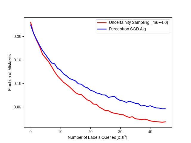
(a) Test Error Comparison.

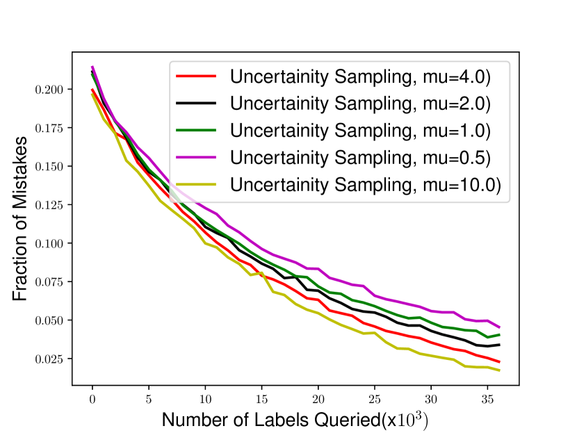
(b) Comparing $\mu$.

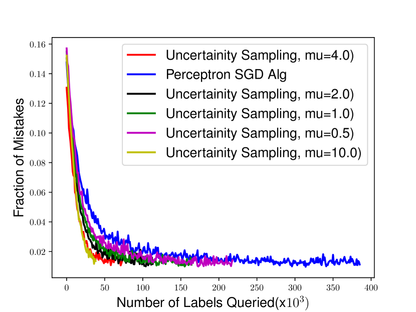
(c) Unlabeled Data Requirement.

Figure 1: Experimental results for binary classification on synthetic data.

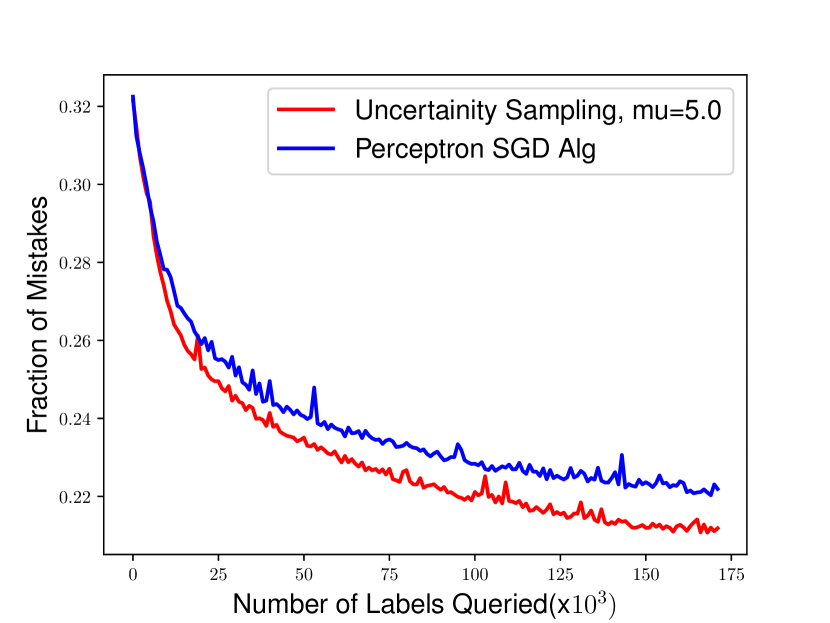
(a) Test Error (Covertype dataset).

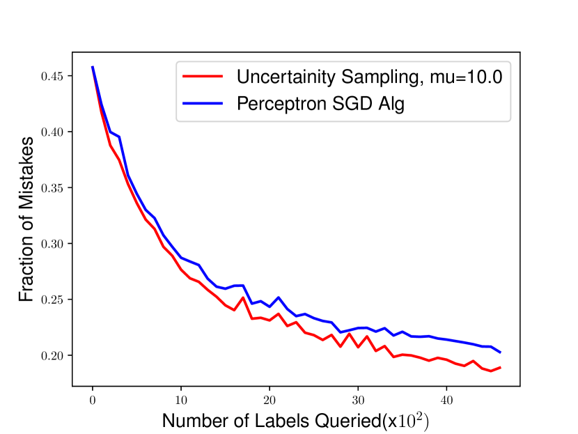
(b) Test Error (letter dataset).

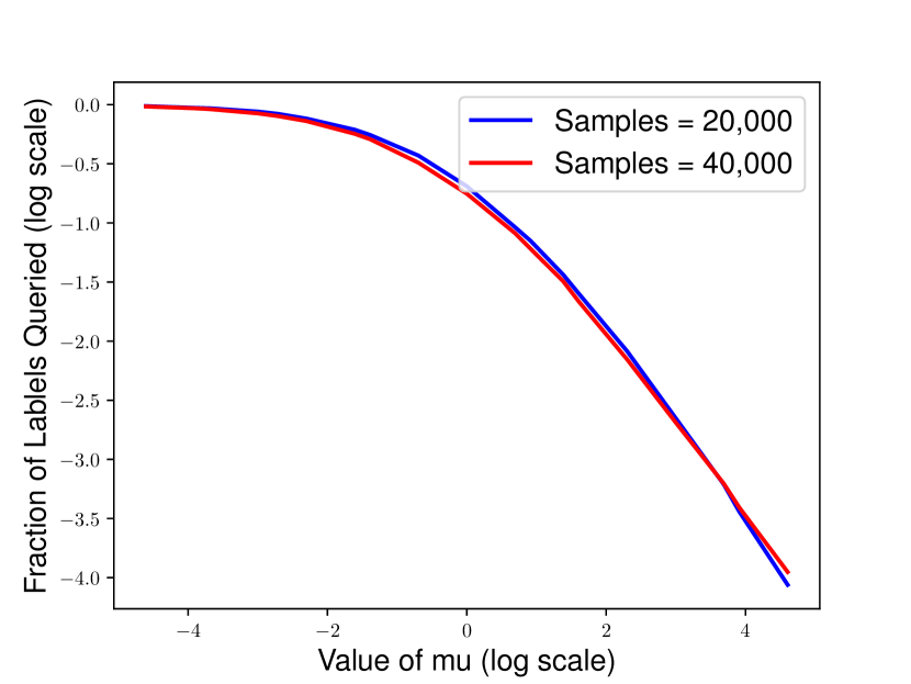
(c) Number of queries vs $\mu$

Figure 2: Experimental results for binary classification.

4 Experiments

In this section, we perform an experimental evaluation for our proposed uncertainty sampling based active learning algorithm. The experiments are performed on both synthetic as well as real world data.

Synthetic Data (Binary Classification).

We generate $n$ number of data points $x_{i}\in\mathbb{R}^{d}$ for $i\in\{1,2,\cdots,n\}$ having dimension $d=200$ from Gaussian distribution centered at 0 with covariance matrix $\Sigma$ which is a diagonal matrix. Similarly, we generate a 200-dimensional prediction vector $\theta$ sampled from the normal distribution. We compute the prediction vector $y_{i}$ for $x_{i}$ as follows, $y_{i}=\mathop{\rm sign}(\theta^{\top}x_{i})$. Separately from the training set, another set of 15,000 data points are generated which are used to evaluate the test performance.

To generate Fig. 1a, we fix $n=200,000$, $\mu=4$ and the $i$-th singular value of $\Sigma$ is ${1}/{i}$. We run one pass of vanilla SGD algorithm and our uncertainty sampling based active learning algorithm. As clear from our plot, out of 200,000 samples, our algorithm asks labels for only 40,000 sample. Hence, for the comparison, we compare the performance on test set of first $40,000$ iteration of vanilla SGD with our algorithm.

In Fig. 1b, we compare the test performance for various $\mu$. It is obvious that larger value of $\mu$ implies a more aggressive sampling scheme. Hence, it is expected that for a fixed budget, larger value of $\mu$ will provide better performance which is also reflected in the plot 1(b).

In Fig. 1c, we plot the test accuracy with respect to the number of labels queries given with fixed budget of unlabeled data. As can be seen from the plot, vanilla SGD asks for the label of every data point. As we increase $\mu$, the number of queried labels goes down. However, the performance on test data remains almost the same surprisingly for uncertainty sampling based algorithm with increasing $\mu$ and for vanilla SGD at the end of one epoch.

Real World Datasets.

Next, we evaluate our algorithm on real world datasets. We consider Covertype and letter-binary datasets to evaluate the test performance of uncertainty sampling based active learning for binary classification. Normalized binary version of datasets are downloaded from   manikvarma.org/code/LDKL/download.html. Since, the decision boundary for these datasets are non-linear, we use randomized Fourier features [18] to perform the task of classification. For both the datasets, we use 500 random fourier feature representation. We perform vanilla SGD and uncertainty sampling based active learning. We plot the result in Fig. 2(a) for covertype and in Fig. 2(b) for letter-binary. We observe that uncertainty sampling based active learning algorithm has low prediction error for a fixed budget.

In the last Fig. 2(c), we plot the fraction of labels queried for various value of $\mu$ when number of unlabeled synthetically generated samples are fixed to 20,000 and 40,000. The plot shows that, our algorithm tends to query similar fraction of labels irrespective of number of available unlabeled data points.

5 Conclusion

In this paper, we show that our uncertainty sampling based active learning method converges to the optimal predictor for linear models under the proposed sampling scheme for binary as well as for multi-class classification. We also extend our analysis for noisy case under restrictive noise assumptions (eqs. (17) and (18)). As a future research direction, we would like to analyze uncertainty sampling algorithm based active learning algorithm under more generalized noise assumptions of Tsybakov [26]),and would like to consider more aggressive sampling schemes.

Acknowledgements

This work was funded in part by the French government under management of Agence Nationale de la Recherche as part of the “Investissements d’avenir” program, reference ANR-19-P3IA-0001 (PRAIRIE 3IA Institute). We also acknowledge support the European Research Council (grant SEQUOIA 724063).

Appendix

Appendix A Binary Separable Classification

Theorem (Restatement of Theorem 1).

Consider a set of $n$ i.i.d samples $(x_{i},y_{i})$ jointly sampled from $\mathcal{P}$ such that $x_{i}\in\mathbb{R}^{d}$, and $y_{i}\in\{-1,1\}$ for all $i=1,\dots,n$ then under the assumption that there exists a $\theta_{\star}$ for which $y(\theta_{\star}^{\top}x)\geq\rho^{\star}$ for all $(x,y)$ pair in $\mathcal{P}$, the following convergence guarantee exists for Algorithm 1,

$${\mathbb{E}}(1-y\theta_{t}^{\top}x)_{+}\leq\frac{R^{2}\max\left\{1,\frac{1}{\mu}\right\}\|\theta_{1}-\theta_{\star}\|^{2}}{\min\left\{\frac{1}{\mu},\frac{\rho^{\star}-1}{1+\mu}\right\}^{2}n},$$ (20)

for the choice of $\sigma(\theta,x)=\frac{1}{1+\mu|\theta^{\top}x|}$, step size $\gamma=\frac{\min\left\{\frac{1}{\mu},\frac{\rho^{\star}-1}{1+\mu}\right\}}{R^{2}\max\left\{1,\frac{1}{\mu}\right\}}$ and $\|x\|\leq R$ for all $x$ in the domain $\mathcal{X}$.

Proof.

We minimize the square hinge loss which can be written as,

$$\ell(x,y,\theta)=\frac{1}{2}\max\left[0,1-y\theta^{\top}x\right]^{2}.$$

We have the following update rule for:

$$\theta_{t+1}=\theta_{t}+\gamma~{}z_{t}(y_{t}x_{t})\big{[}1-y_{t}({\theta_{t}}^{\top}x_{t})\big{]}_{+}$$

where $z_{t}$ is a bernoulli random variable for fixed $\theta_{t}$ and $x_{t}$ such that $p(z_{t}=1|x_{t},\theta_{t})=\sigma(\theta_{t},x_{t})$ where $\sigma:\mathbb{R}^{d}\times\mathbb{R}^{d}\rightarrow[0,1]$ is an even function. Following the update, we have

$$\begin{split}\left\|\theta_{t+1}-\theta^{\star}\right\|^{2}&=\left\|\theta_{t}-\theta^{\star}+\gamma~{}z_{t}(y_{t}x_{t})\big{[}1-y_{t}({\theta_{t}}^{\top}x_{t})\big{]}_{+}\right\|^{2}\\ &=\left\|\theta_{t}-\theta^{\star}\right\|^{2}+2\gamma z_{t}\big{[}1-y_{t}({\theta_{t}}^{\top}x_{t})\big{]}_{+}\left(y_{t}(\theta_{t}^{\top}x_{t})-y_{t}({\theta^{\star}}^{\top}x_{t})\right)+\gamma^{2}z_{t}^{2}(y_{t}x_{t})^{2}\big{[}1-y_{t}({\theta_{t}}^{\top}x_{t})\big{]}_{+}^{2}\\ &=\left\|\theta_{t}-\theta^{\star}\right\|^{2}+2\gamma z_{t}\big{[}1-y_{t}({\theta_{t}}^{\top}x_{t})\big{]}_{+}\left(y_{t}(\theta_{t}^{\top}x_{t})-y_{t}({\theta^{\star}}^{\top}x_{t})\right)+\gamma^{2}z_{t}(y_{t}x_{t})^{2}\big{[}1-y_{t}({\theta_{t}}^{\top}x_{t})\big{]}_{+}^{2}\end{split}$$ (21)

In the last equation we used the fact that $z_{t}\in\{0,1\}$, hence $z_{t}^{2}=z_{t}$. Taking expectations on both sides only with respect to $z_{t}$ considering $(x_{t},y_{t},\theta_{t})$ fixed, we have

$${\mathbb{E}}\|\theta_{t+1}-\theta^{\star}\|^{2} =\|\theta_{t}-\theta^{\star}\|^{2}+2\gamma\sigma(\theta_{t},x_{t})\big{[}1-y_{t}({\theta_{t}}^{\top}x_{t})\big{]}_{+}\left(y_{t}(\theta_{t}^{\top}x_{t})-y_{t}({\theta^{\star}}^{\top}x_{t})\right)$$

$$\qquad\qquad\qquad\qquad\qquad\qquad\qquad\qquad\qquad+\gamma^{2}\sigma(\theta_{t},x_{t})\|y_{t}x_{t}\|^{2}\big{[}1-y_{t}({\theta_{t}}^{\top}x_{t})\big{]}_{+}^{2}$$

$$\leq\|\theta_{t}-\theta^{\star}\|^{2}+2\gamma\sigma(\theta_{t}^{\top}x_{t})\big{[}1-y_{t}({\theta_{t}}^{\top}x_{t})\big{]}_{+}\left(y_{t}(\theta_{t}^{\top}x_{t})-y_{t}({\theta^{\star}}^{\top}x_{t})\right)$$

$$\qquad\qquad\qquad\qquad\qquad\qquad\qquad\qquad\qquad+\gamma^{2}\sigma(\theta_{t}^{\top}x_{t})R^{2}\big{[}1-y_{t}({\theta_{t}}^{\top}x_{t})\big{]}_{+}^{2}.$$ (22)

Now in the above equation, we want to find function $\sigma:\mathbb{R}^{d}\times\mathbb{R}^{d}\rightarrow[0,1]$ for $y_{t}(\theta_{t}^{\top}x_{t})<1$ for all $t$, such that the following holds,

$$\sigma(\theta_{t},x_{t})(1-y_{t}\theta_{t}^{\top}x_{t})_{+}^{2}\leq c_{1}(1-y_{t}\theta_{t}^{\top}x_{t})_{+}$$

$$\sigma(\theta_{t},x_{t})(1-y_{t}\theta_{t}^{\top}x_{t})_{+}(y_{t}\theta_{t}^{\top}x_{t}-y_{t}{\theta^{\star}}^{\top}x_{t})\leq-c_{2}(1-y_{t}\theta_{t}^{\top}x_{t})_{+}$$

for some positive constants $c_{1}$ and $c_{2}$. This is then equivalent to, for all $y_{t}\theta_{t}^{\top}x_{t}<1$ and $y_{t}{\theta_{\star}}^{\top}x_{t}\geq\rho^{\star}$:

$$\sigma(\theta_{t},x_{t})(1-y_{t}\theta_{t}^{\top}x_{t})_{+} \leq c_{1}$$ (23)

$$\sigma(\theta_{t},x_{t})(\rho^{\star}-y_{t}\theta_{t}^{\top}x_{t}) \geq c_{2}$$ (24)

IF we choose, $\sigma(\theta,x)=\frac{1}{1+\mu|\theta^{\top}x|}$ for some constant $\mu>0$, then from lemma 1, we have

$$\frac{\min\left\{\frac{1}{\mu},\frac{\rho^{\star}-1}{1+\mu}\right\}}{(\rho^{\star}-y\theta^{\top}x)}\leq\sigma(\theta,x)\leq\frac{\max\left\{1,\frac{1}{\mu}\right\}}{(1-y\theta^{\top}x)_{+}}.$$

Hence, we have

$${\mathbb{E}}\|\theta_{t+1}-\theta^{\star}\|^{2}\leq\|\theta_{t}-\theta^{\star}\|^{2}-2\gamma\min\left\{\frac{1}{\mu},\frac{\rho^{\star}-1}{1+\mu}\right\}(1-y_{t}\theta_{t}^{\top}x_{t})_{+}+\gamma^{2}R^{2}\max\left\{1,\frac{1}{\mu}\right\}(1-y_{t}\theta_{t}^{\top}x_{t})_{+}$$

$$\Rightarrow~{} (1-y_{t}\theta_{t}^{\top}x_{t})_{+}\leq\frac{1}{2\gamma\min\left\{\frac{1}{\mu},\frac{\rho^{\star}-1}{1+\mu}\right\}-\gamma^{2}R^{2}\max\left\{1,\frac{1}{\mu}\right\}}\left[\|\theta_{t}-\theta^{\star}\|^{2}-{\mathbb{E}}\|\theta_{t+1}-\theta^{\star}\|^{2}\right]$$

Taking expectation on both the sides, we have

$$(1-y\theta_{t}^{\top}x)_{+}\leq\frac{1}{2\gamma\min\left\{\frac{1}{\mu},\frac{\rho^{\star}-1}{1+\mu}\right\}-\gamma^{2}R^{2}\max\left\{1,\frac{1}{\mu}\right\}}\left[\|\theta_{t}-\theta^{\star}\|^{2}-{\mathbb{E}}\|\theta_{t+1}-\theta^{\star}\|^{2}\right]$$ (25)

Summing the above equation for $t=1$ to $n$, choosing $\gamma=\frac{\min\left\{\frac{1}{\mu},\frac{\rho^{\star}-1}{1+\mu}\right\}}{R^{2}\max\left\{1,\frac{1}{\mu}\right\}}$ and applying Jensen’s inequality give us,

$${\mathbb{E}}(1-y\theta_{t}^{\top}x)_{+}\leq\frac{R^{2}\max\left\{1,\frac{1}{\mu}\right\}\|\theta_{1}-\theta_{\star}\|^{2}}{\min\left\{\frac{1}{\mu},\frac{\rho^{\star}-1}{1+\mu}\right\}^{2}n}.$$ (26)

∎

Lemma 1.

If there exist a function $\sigma:\mathbb{R}^{d}\times\mathbb{R}^{d}\rightarrow\mathbb{R}$ of the form,

$$\sigma(\theta,x)=\frac{1}{1+\mu|\theta^{\top}x|}$$ (27)

where $\theta\in\mathbb{R}^{d}$ and $x\in\mathbb{R}^{d}$, then under the assumptions of theorem 1 we have

$$\frac{\min\left\{\frac{1}{\mu},\frac{\rho^{\star}-1}{1+\mu}\right\}}{(\rho^{\star}-y\theta^{\top}x)}\leq\sigma(\theta,x)\leq\frac{\max\left\{1,\frac{1}{\mu}\right\}}{(1-y\theta^{\top}x)_{+}}$$ (28)

for all $y(\theta^{\top}x)\leq 1$ where $y\in\{-1,1\}$.

Proof.

We want to find an even function $\sigma:\mathbb{R}^{d}\times\mathbb{R}^{d}\to[0,1]$, such that for all $y(\theta^{\top}x)\leq 1$ where $y\in\{-1,1\}$, the following conditions hold

$$\sigma(\theta,x)(1-y\theta^{\top}x)_{+} \leq c_{1}$$

$$\sigma(\theta,x)(y\theta^{\top}x-\rho^{\star}) \leq-c_{2}$$

for some positive constants $c_{1}$ and $c_{2}$ and $\frac{c_{1}}{c_{2}^{2}}$ is as small as possible. Replacing $\sigma(\theta,x)$ with $\frac{1}{1+\mu|\theta^{\top}x|}$ and using the fact that $y\theta^{\top}x\leq 1$, we get to find constants $c_{1}$ and $c_{2}$ such that

$$c_{1} \geq\frac{1-y\theta^{\top}x}{1+\mu|\theta^{\top}x|},$$

$$c_{2} \leq\frac{\rho^{\star}-y\theta^{\top}x}{1+\mu|\theta^{\top}x|}.$$

When $\mu\geq\frac{1}{\rho^{\star}}$, $\frac{\rho^{\star}-u}{1+\mu|u|}$ is decreasing function for $u>0$ and increasing function for $u\leq 0$. When $\mu\leq\frac{1}{\rho^{\star}}$, $\frac{\rho^{\star}-u}{1+\mu|u|}$ is a decreasing function everywhere. Checking at $y\theta^{\top}x=0$, $y\theta^{\top}x=1$ and $y\theta^{\top}x\rightarrow-\infty$, we have

$$c_{1}\geq\max{\left\{1,\frac{1}{\mu}\right\}}~{}\text{and}~{}c_{2}\leq\min\left\{\frac{1}{\mu},\frac{\rho^{\star}-1}{1+\mu}\right\}.$$

Hence, finally we have

$$\frac{\min\left\{\frac{1}{\mu},\frac{\rho^{\star}-1}{1+\mu}\right\}}{(\rho^{\star}-y\theta^{\top}x)}\leq\sigma(\theta,x)\leq\frac{\max\left\{1,\frac{1}{\mu}\right\}}{(1-y\theta^{\top}x)_{+}}.$$ (29)

∎

Appendix B Separable Multi-class Classification

Theorem (Restatement of Theorem 2).

Consider a set of $n$ i.i.d samples $(x_{i},y_{i})$ jointly sampled from $\mathcal{P}$ such that $x_{i}\in\mathbb{R}^{d}$, and $y_{i}\in\{1,2,\ldots,k\}$ for all $i=1,\dots,n$ then under the assumption that there exists a set of $d$-dimensional optimal half-spaces $\theta_{\star}=\{\theta_{\star}(1),\theta_{\star}(2),\ldots,\theta_{\star}(k)\}$ corresponding to each class for which $\theta_{\star}^{\top}\delta_{x}(y,y^{\star}(\theta_{\star},x,y))\geq\rho^{\star}$ for all $(x,y)$ pair in $\mathcal{P}$, the following convergence guarantee exists for Algorithm 2 under projected gradient descent update in equation (11),

$${\mathbb{E}}\hat{\ell}(x,y,\bar{\theta}_{n})\leq\frac{R^{2}(1+BR)\|\theta_{1}-\theta_{\star}\|^{2}}{\min\left\{\frac{1}{\mu},\frac{\rho^{\star}-1}{1+\mu}\right\}^{2}n},$$ (30)

for the choice of $\sigma(\theta,x)=\frac{1}{1+\mu\left|\theta_{t}(y_{t(1)}^{\star})^{\top}x_{t}-\theta_{t}(y_{t(2)}^{\star})^{\top}x_{t}\right|}$, step size $\gamma=\min\left\{\frac{1}{\mu},\frac{\rho^{\star}-1}{1+\mu}\right\}\frac{1}{R^{2}(1+BR)}$ and $\|\delta_{x}(i,j)\|\leq R$ for all $x$ in the domain $\mathcal{X}$, and for all $i\neq j\in[k]$ and $\|\theta\|\leq B$.

Proof.

We have multi-class hinge loss,

$$\hat{\ell}(x_{t},y_{t},\theta)=\left[1-\theta^{\top}\delta_{x_{t}}\left(y_{t},y^{\star}(\theta,x_{t},y_{t})\right)\right]_{+},~{}\text{where}~{}~{}y^{\star}(\theta,x_{t},y_{t})=\mathop{\rm arg\,max}_{y\in{\mathcal{Y}\backslash{y_{t}}}}\theta^{\top}\phi(x_{t},y),$$

and $\phi(x,y)\in\mathbb{R}^{dk}$ represents the feature map corresponding to the sample $(x,y)$. We have assumed that

$${\theta^{\star}}^{\top}\delta_{x_{t}}\left(y_{t},y^{\star}(\theta,x_{t},y_{t})\right)\geq\rho^{\star}\geq 1~{}~{}\text{for all}~{}~{}t.$$

Let us consider the smooth loss function,

$${\ell}(x_{t},y_{t},\theta)=\left[\hat{\ell}(x_{t},y_{t},\theta)\right]^{2}=\left[1-\theta^{\top}\delta_{x_{t}}\left(y_{t},y^{\star}(\theta,x_{t},y_{t})\right)\right]_{+}^{2}.$$

We perform the following projected stochastic update

$$\theta_{t+1}=\Pi_{\|\theta\|\leq B}\left[\theta_{t}+\gamma z_{t}\delta_{x_{t}}\left(y_{t},y^{\star}(\theta_{t},x_{t},y_{t})\right)\left[1-\theta^{\top}\delta_{x_{t}}\left(y_{t},y^{\star}(\theta,x_{t},y_{t})\right)\right]_{+}\right]$$

where $z_{t}$ is a bernoulli random variable such that $p(z_{t}=1|x_{t},\theta_{t})=\sigma(\theta_{t},\top x_{t})$ such that $\sigma:\mathbb{R}^{dk}\times\mathbb{R}^{dk}\rightarrow[0,1]$ is an even function. Now,

$$\begin{split}\left\|\theta_{t+1}-\theta^{\star}\right\|^{2}&\leq\left\|\theta_{t}-\theta^{\star}+\gamma z_{t}\delta_{x_{t}}\left(y_{t},y^{\star}(\theta,x_{t},y_{t})\right)\left[1-\theta^{\top}\delta_{x_{t}}\left(y_{t},y^{\star}(\theta_{t},x_{t},y_{t})\right)\right]_{+}\right\|^{2}\\ &=\left\|\theta_{t}-\theta^{\star}\right\|^{2}+2\gamma z_{t}\hat{\ell}(x_{t},y_{t},\theta_{t})\left(\theta_{t}^{\top}\delta_{x_{t}}\left(y_{t},y^{\star}(\theta_{t},x_{t},y_{t})\right)-{\theta^{\star}}^{\top}\delta_{x_{t}}\left(y_{t},y^{\star}(\theta_{t},x_{t},y_{t})\right))\right)\\ &\qquad\qquad\qquad\qquad+\gamma^{2}z_{t}^{2}\|\delta_{x_{t}}\left(y_{t},y^{\star}(\theta_{t},x_{t},y_{t})\right)\|^{2}\hat{\ell}^{2}(x_{t},y_{t},\theta_{t})\\ &=\left\|\theta_{t}-\theta^{\star}\right\|^{2}+2\gamma z_{t}\hat{\ell}(x_{t},y_{t},\theta_{t})\left(\theta_{t}^{\top}\delta_{x_{t}}\left(y_{t},y^{\star}(\theta_{t},x_{t},y_{t})\right)-{\theta^{\star}}^{\top}\delta_{x_{t}}\left(y_{t},y^{\star}(\theta_{t},x_{t},y_{t})\right))\right)\\ &\qquad\qquad\qquad\qquad+\gamma^{2}z_{t}\|\delta_{x_{t}}\left(y_{t},y^{\star}(\theta_{t},x_{t},y_{t})\right)\|^{2}\hat{\ell}^{2}(x_{t},y_{t},\theta_{t}).\end{split}$$ (31)

In the last equation we used the fact that $z_{t}\in\{0,1\}$, hence $z_{t}^{2}=z_{t}$. Taking expectations on both sides only with respect to $z_{t}$ considering $(x_{t},y_{t},\theta_{t})$ fixed, we have

$${\mathbb{E}}\|\theta_{t+1}-\theta^{\star}\|^{2} \leq\left\|\theta_{t}-\theta^{\star}\right\|^{2}+2\gamma\sigma(\theta_{t},x_{t})\hat{\ell}(x_{t},y_{t},\theta_{t})\left(\theta_{t}^{\top}\delta_{x_{t}}\left(y_{t},y^{\star}(\theta_{t},x_{t},y_{t})\right)-{\theta^{\star}}^{\top}\delta_{x_{t}}\left(y_{t},y^{\star}(\theta_{t},x_{t},y_{t})\right))\right)$$

$$\qquad\qquad\qquad\qquad+\gamma^{2}\sigma(\theta_{t},x_{t})\|\delta_{x_{t}}\left(y_{t},y^{\star}(\theta_{t},x_{t},y_{t})\right)\|^{2}\hat{\ell}^{2}(x_{t},y_{t},\theta_{t})$$

$$\leq\|\theta_{t}-\theta^{\star}\|^{2}+2\gamma\sigma(\theta_{t},x_{t})\hat{\ell}(x_{t},y_{t},\theta_{t})\left(\theta_{t}^{\top}\delta_{x_{t}}\left(y_{t},y^{\star}(\theta_{t},x_{t},y_{t})\right)-{\theta^{\star}}^{\top}\delta_{x_{t}}\left(y_{t},y^{\star}(\theta_{t},x_{t},y_{t})\right))\right)$$

$$\qquad\qquad\qquad\qquad\qquad\qquad\qquad\qquad\qquad+\gamma^{2}\sigma(\theta_{t},x_{t})R^{2}\hat{\ell}^{2}(x_{t},y_{t},\theta_{t})$$

$$\leq\|\theta_{t}-\theta^{\star}\|^{2}+2\gamma\sigma(\theta_{t},x_{t})\hat{\ell}(x_{t},y_{t},\theta_{t})\left(\theta_{t}^{\top}\delta_{x_{t}}\left(y_{t},y^{\star}(\theta_{t},x_{t},y_{t})\right)-\rho^{\star}\right)$$

$$\qquad\qquad\qquad\qquad\qquad\qquad\qquad\qquad\qquad+\gamma^{2}\sigma(\theta_{t},x_{t})R^{2}\hat{\ell}^{2}(x_{t},y_{t},\theta_{t})$$ (32)

Now, we want to choose such a function $\sigma$ for $\hat{\ell}(x_{t},y_{t},\theta_{t})>0$ such that

$$\sigma(\theta_{t},x_{t})\hat{\ell}^{2}(x_{t},y_{t},\theta_{t})\leq c_{1}\hat{\ell}(x_{t},y_{t},\theta_{t})$$

$$\sigma(\theta_{t},x_{t})\left(\rho^{\star}-\theta_{t}^{\top}\delta_{x_{t}}\left(y_{t},y^{\star}(\theta_{t},x_{t},y_{t})\right)\right)\geq c_{2}$$

for some positive constants $c_{1}$ and $c_{2}$. If we choose,

$$\sigma(\theta,x)=\frac{1}{1+\mu\left|\theta_{t}(y_{t(1)}^{\star})^{\top}x_{t}-\theta_{t}(y_{t(2)}^{\star})^{\top}x_{t}\right|},$$

the from lemma 2 we have,

$$\sigma(\theta_{t},x_{t}) \leq\frac{1+BR}{\hat{\ell}(x_{t},y_{t},\theta_{t})},$$

$$\sigma(\theta_{t},x_{t}) \geq\min\left\{\frac{1}{\mu},\frac{\rho^{\star}-1}{1+\mu}\right\}\frac{1}{\left(\rho^{\star}-\theta_{t}^{\top}\delta_{x_{t}}\left(y_{t},y^{\star}(\theta_{t},x_{t},y_{t})\right)\right)}.$$ (33)

Putting the inequalities in equation (33) back in the equation (32), we get the following,

$${\mathbb{E}}\|\theta_{t+1}-\theta^{\star}\|^{2}\leq\|\theta_{t}-\theta^{\star}\|^{2}-2\gamma\min\left\{\frac{1}{\mu},\frac{\rho^{\star}-1}{1+\mu}\right\}\hat{\ell}(x_{t},y_{t},\theta_{t})+\gamma^{2}R^{2}(1+BR)\hat{\ell}(x_{t},y_{t},\theta_{t})$$

$$\Rightarrow~{} \hat{\ell}(x_{t},y_{t},\theta_{t})\leq\frac{1}{2\gamma\min\left\{\frac{1}{\mu},\frac{\rho^{\star}-1}{1+\mu}\right\}-\gamma^{2}R^{2}(1+BR)}\left[\|\theta_{t}-\theta^{\star}\|^{2}-{\mathbb{E}}\|\theta_{t+1}-\theta^{\star}\|^{2}\right]$$

Taking expectation on both the sides, we have

$$\hat{\ell}(x,y,\theta_{t})\leq\frac{1}{2\gamma\min\left\{\frac{1}{\mu},\frac{\rho^{\star}-1}{1+\mu}\right\}-\gamma^{2}R^{2}(1+BR)}\left[{\mathbb{E}}\|\theta_{t}-\theta^{\star}\|^{2}-{\mathbb{E}}\|\theta_{t+1}-\theta^{\star}\|^{2}\right]$$ (34)

Summing the above equation for $t=1$ to $n$, choosing $\gamma=\min\left\{\frac{1}{\mu},\frac{\rho^{\star}-1}{1+\mu}\right\}\frac{1}{R^{2}(1+BR)}$ and applying Jensen’s inequality give us,

$${\mathbb{E}}\hat{\ell}(x,y,\bar{\theta}_{n})\leq\frac{R^{2}(1+BR)\|\theta_{1}-\theta_{\star}\|^{2}}{\min\left\{\frac{1}{\mu},\frac{\rho^{\star}-1}{1+\mu}\right\}^{2}n}.$$ (35)

∎

Lemma 2.

Consider the setting and notations of theorem 2. If there exist a function $\sigma:\mathbb{R}^{dk}\times\mathbb{R}^{dk}\rightarrow\mathbb{R}$ of the form,

$$\sigma(\theta,x)=\frac{1}{1+\mu\left|\theta(y_{(1)}^{\star})^{\top}x-\theta(y_{(2)}^{\star})^{\top}x\right|}$$ (36)

where $\theta\in\mathbb{R}^{dk}$ and $x\in\mathbb{R}^{dk}$, then under the assumptions of theorem 2 we have

$$\min\left\{\frac{1}{\mu},\frac{\rho^{\star}-1}{1+\mu}\right\}\frac{1}{\left(\rho^{\star}-\theta^{\top}\delta_{x}\left(y,y^{\star}(\theta,x,y)\right)\right)}\leq\sigma(\theta,x)\leq\frac{1+BR}{\hat{\ell}(x,y,\theta)}$$ (37)

for all $\theta^{\top}\delta_{x}\left(y,y^{\star}(\theta,x,y)\right)\leq 1$ where $y\in\{1,2,\ldots,k\}$.

Proof.

We want to find an even function $\sigma:\mathbb{R}^{d}\times\mathbb{R}^{d}\to[0,1]$, such that for all $y(\theta^{\top}x)\leq 1$ where $y\in\{-1,1\}$, the following conditions hold

$$\sigma(\theta_{t},x_{t})\hat{\ell}^{2}(x_{t},y_{t},\theta_{t})\leq c_{1}\hat{\ell}(x_{t},y_{t},\theta_{t})$$

$$\sigma(\theta_{t},x_{t})\left(\rho^{\star}-\theta_{t}^{\top}\delta_{x_{t}}\left(y_{t},y^{\star}(\theta_{t},x_{t},y_{t})\right)\right)\geq c_{2}$$

for some positive constants $c_{1}$ and $c_{2}$ and $\frac{c_{1}}{c_{2}^{2}}$ is as small as possible. Replacing $\sigma(\theta,x)$ with $\frac{1}{1+\mu\left|\theta(y_{(1)}^{\star})^{\top}x-\theta(y_{(2)}^{\star})^{\top}x\right|}$ and using the fact that $\hat{\ell}(x_{t},y_{t},\theta_{t})y>0$, we get to find constants $c_{1}$ and $c_{2}$ such that

$$c_{1}\geq\frac{\hat{\ell}(x_{t},y_{t},\theta_{t})}{1+\mu\left|\theta_{t}(y_{t(1)}^{\star})^{\top}x_{t}-\theta_{t}(y_{t(2)}^{\star})^{\top}x_{t}\right|}$$ (38)

$$c_{2}\leq\frac{\rho^{\star}-\theta_{t}^{\top}\delta_{x_{t}}\left(y_{t},y^{\star}(\theta_{t},x_{t},y_{t})\right)}{1+\mu\left|\theta_{t}(y_{t(1)}^{\star})^{\top}x_{t}-\theta_{t}(y_{t(2)}^{\star})^{\top}x_{t}\right|}$$ (39)

Under bounded $\theta$ assumption we have,

$$\frac{\hat{\ell}(x_{t},y_{t},\theta_{t})}{1+\mu\left|\theta_{t}(y_{t(1)}^{\star})^{\top}x_{t}-\theta(y_{t(2)}^{\star})^{\top}x_{t}\right|}\leq 1+BR.$$ (40)

In the above equation, we have used cauchy-shwartz inequality, $\|\theta\|\leq B$ and $\|\delta_{x}(i,j)\|\leq R$ for all $x\in\mathcal{X}$ and $i,j\in[k]$. Let us now consider to get the inequality for $c_{2}$. We here observe that

$$\left|\theta_{t}(y_{t(1)}^{\star})^{\top}x_{t}-\theta_{t}(y_{t(2)}^{\star})^{\top}x_{t}\right|\leq\left|\theta_{t}^{\top}\delta_{x_{t}}\left(y_{t},y^{\star}(\theta_{t},x_{t},y_{t})\right)\right|$$

Hence,

$$\frac{\rho^{\star}-\theta_{t}^{\top}\delta_{x_{t}}\left(y_{t},y^{\star}(\theta_{t},x_{t},y_{t})\right)}{1+\mu\left|\theta_{t}^{\top}\delta_{x_{t}}\left(y_{t},y^{\star}(\theta_{t},x_{t},y_{t})\right)\right|}\leq\frac{\rho^{\star}-\theta_{t}^{\top}\delta_{x_{t}}\left(y_{t},y^{\star}(\theta_{t},x_{t},y_{t})\right)}{1+\mu\left|\theta_{t}(y_{t(1)}^{\star})^{\top}x_{t}-\theta_{t}(y_{t(2)}^{\star})^{\top}x_{t}\right|}$$

When $\mu\geq\frac{1}{\rho^{\star}}$, $\frac{\rho^{\star}-u}{1+\mu|u|}$ is decreasing function for $u>0$ and increasing function for $u\leq 0$. When $\mu\leq\frac{1}{\rho^{\star}}$, $\frac{\rho^{\star}-u}{1+\mu|u|}$ is a decreasing function everywhere. Hence, checking the value at $\theta_{t}^{\top}\delta_{x_{t}}\left(y_{t},y^{\star}(\theta_{t},x_{t},y_{t})\right)=1$ and $\theta_{t}^{\top}\delta_{x_{t}}\left(y_{t},y^{\star}(\theta_{t},x_{t},y_{t})\right)\rightarrow-\infty$ gives us the following,

$$c_{2}\leq\min\left\{\frac{1}{\mu},\frac{\rho^{\star}-1}{1+\mu}\right\}\leq\frac{\rho^{\star}-\theta_{t}^{\top}\delta_{x_{t}}\left(y_{t},y^{\star}(\theta_{t},x_{t},y_{t})\right)}{1+\mu\left|\theta_{t}(y_{t(1)}^{\star})^{\top}x_{t}-\theta_{t}(y_{t(2)}^{\star})^{\top}x_{t}\right|}.$$

Hence, we have

$$\min\left\{\frac{1}{\mu},\frac{\rho^{\star}-1}{1+\mu}\right\}\frac{1}{\left(\rho^{\star}-\theta_{t}^{\top}\delta_{x_{t}}\left(y_{t},y^{\star}(\theta_{t},x_{t},y_{t})\right)\right)}\leq\sigma(\theta_{t},x_{t})\leq\frac{1+BR}{\hat{\ell}(x_{t},y_{t},\theta_{t})}.$$ (41)

∎

Appendix C Binary Classification in the Presence of Noise

Lemma 3.

Under the assumption in equation (17), the iterates in algorithm 1 updated via stochastic gradient descent (equation (4)) or projected stochastic gradient descent (equation (19)) satisfy

$${\mathbb{E}}\left\|\theta_{t+1}-\theta^{\star}\right\|^{2} \leq{\mathbb{E}}\left\|\theta_{t}-\theta^{\star}\right\|^{2}-2\gamma(1-\eta)\min\left\{\frac{1}{\mu},\frac{\rho^{\star}-1}{1+\mu}\right\}{\mathbb{E}}(1-y\theta_{t}^{\top}x)_{+}$$

$$\qquad+2\gamma\eta~{}\max\left\{\frac{1+R\|\theta_{\star}\|}{1+\mu},R\|\theta_{\star}\|\right\}{\mathbb{E}}(1-y\theta_{t}^{\top}x)_{+}+\gamma^{2}R^{2}\max\left\{1,\frac{1}{\mu}\right\}{\mathbb{E}}(1-y\theta_{t}^{\top}x)_{+}$$ (42)

for the choice of $\sigma(\theta,x)=\frac{1}{1+\mu|\theta^{\top}x|}$, $\mu>0$, and positive step size $\gamma$ such that for all $\|x\|\leq R$ for all $x\in\mathcal{X}$.

Proof.

$$\begin{split}\left\|\theta_{t+1}-\theta^{\star}\right\|^{2}&=\left\|\theta_{t}-\theta^{\star}+\gamma~{}z_{t}(y_{t}x_{t})\big{[}1-y_{t}({\theta_{t}}^{\top}x_{t})\big{]}_{+}\right\|^{2}\\ &=\left\|\theta_{t}-\theta^{\star}\right\|^{2}+2\gamma z_{t}\big{[}1-y_{t}({\theta_{t}}^{\top}x_{t})\big{]}_{+}\left(y_{t}(\theta_{t}^{\top}x_{t})-y_{t}({\theta^{\star}}^{\top}x_{t})\right)+\gamma^{2}z_{t}^{2}(y_{t}x_{t})^{2}\big{[}1-y_{t}({\theta_{t}}^{\top}x_{t})\big{]}_{+}^{2}\\ &=\left\|\theta_{t}-\theta^{\star}\right\|^{2}+2\gamma z_{t}\big{[}1-y_{t}({\theta_{t}}^{\top}x_{t})\big{]}_{+}\left(y_{t}(\theta_{t}^{\top}x_{t})-y_{t}({\theta^{\star}}^{\top}x_{t})\right)+\gamma^{2}z_{t}(y_{t}x_{t})^{2}\big{[}1-y_{t}({\theta_{t}}^{\top}x_{t})\big{]}_{+}^{2}\end{split}$$ (43)

In the last equation we used the fact that $z_{t}\in\{0,1\}$, hence $z_{t}^{2}=z_{t}$. Taking expectations on both sides only with respect to $z_{t}$ considering $(x_{t},y_{t},\theta_{t})$ fixed, we have

$${\mathbb{E}}\|\theta_{t+1}-\theta^{\star}\|^{2} \leq\|\theta_{t}-\theta^{\star}\|^{2}+2\gamma\sigma(\theta_{t}^{\top}x_{t})\big{[}1-y_{t}({\theta_{t}}^{\top}x_{t})\big{]}_{+}\left(y_{t}(\theta_{t}^{\top}x_{t})-y_{t}({\theta^{\star}}^{\top}x_{t})\right)$$

$$\qquad\qquad\qquad\qquad\qquad\qquad\qquad\qquad\qquad+\gamma^{2}\sigma(\theta_{t}^{\top}x_{t})(y_{t}x_{t})^{2}\big{[}1-y_{t}({\theta_{t}}^{\top}x_{t})\big{]}_{+}^{2}$$

$$\leq\|\theta_{t}-\theta^{\star}\|^{2}+2\gamma\sigma(\theta_{t}^{\top}x_{t})\big{[}1-y_{t}({\theta_{t}}^{\top}x_{t})\big{]}_{+}\left(y_{t}(\theta_{t}^{\top}x_{t})-y_{t}({\theta^{\star}}^{\top}x_{t})\right)$$

$$\qquad\qquad\qquad\qquad\qquad\qquad\qquad\qquad\qquad+\gamma^{2}\sigma(\theta_{t}^{\top}x_{t})R^{2}\big{[}1-y_{t}({\theta_{t}}^{\top}x_{t})\big{]}_{+}^{2}.$$ (44)

In the last line, we used the fact that $\|x\|\leq R$ for all $x\in\mathcal{X}$. Now finally we take the expectation with respect to the noise in $y_{t}$, using the assumption made in eq. 17 and conditioning on $\theta_{t}$, $x_{t}$ and $y_{t}$. We get the following,

$${\mathbb{E}}\left\|\theta_{t+1}-\theta^{\star}\right\|^{2} \leq\left\|\theta_{t}-\theta^{\star}\right\|^{2}-2\gamma(1-\eta)\sigma(\theta_{t},x_{t})\big{[}1-y_{t}({\theta_{t}}^{\top}x_{t})\big{]}_{+}\left[\left(y_{t}(\theta_{t}^{\top}x_{t})-\rho^{\star})\right)\right]$$

$$+2\gamma\eta\sigma(\theta_{t},x_{t})\big{[}1-y_{t}({\theta_{t}}^{\top}x_{t})\big{]}_{+}\left[y_{t}(\theta_{t}^{\top}x_{t})+|{\theta^{\star}}^{\top}x_{t}|\right]+\gamma^{2}R^{2}\sigma(\theta_{t},x_{t})\big{[}1-y_{t}({\theta_{t}}^{\top}x_{t})\big{]}_{+}^{2}$$

$$\leq\left\|\theta_{t}-\theta^{\star}\right\|^{2}-2\gamma(1-\eta)\sigma(\theta_{t},x_{t})\big{[}1-y_{t}({\theta_{t}}^{\top}x_{t})\big{]}_{+}\left[\left(y_{t}(\theta_{t}^{\top}x_{t})-\rho^{\star})\right)\right]$$

$$+2\gamma\eta\sigma(\theta_{t},x_{t})\big{[}1-y_{t}({\theta_{t}}^{\top}x_{t})\big{]}_{+}\left[y_{t}(\theta_{t}^{\top}x_{t})+R\|{\theta^{\star}}\|\right]+\gamma^{2}R^{2}\sigma(\theta_{t},x_{t})\big{[}1-y_{t}({\theta_{t}}^{\top}x_{t})\big{]}_{+}^{2}.$$ (45)

Similar to the noiseless case, we choose

$$\sigma(\theta,x)=\frac{1}{1+\mu|\theta^{\top}x|},$$

for $\mu>0$ and after applying result from lemma 1, we have for $y_{t}\theta_{t}^{\top}x_{t}<1$

$${\mathbb{E}}\left\|\theta_{t+1}-\theta^{\star}\right\|^{2} \leq\left\|\theta_{t}-\theta^{\star}\right\|^{2}-2\gamma(1-\eta)\min\left\{\frac{1}{\mu},\frac{\rho^{\star}-1}{1+\mu}\right\}(1-y_{t}\theta_{t}^{\top}x_{t})_{+}$$

$$\qquad\qquad+2\gamma\eta\frac{y_{t}\theta_{t}^{\top}x_{t}+|\theta_{\star}^{\top}x_{t}|}{1+\mu|\theta_{t}^{\top}x_{t}|}(1-y_{t}\theta_{t}^{\top}x_{t})_{+}+\gamma^{2}R^{2}\max\left\{1,\frac{1}{\mu}\right\}(1-y_{t}\theta_{t}^{\top}x_{t})_{+}$$

$$\leq\left\|\theta_{t}-\theta^{\star}\right\|^{2}-2\gamma(1-\eta)\min\left\{\frac{1}{\mu},\frac{\rho^{\star}-1}{1+\mu}\right\}(1-y_{t}\theta_{t}^{\top}x_{t})_{+}$$

$$\qquad\qquad+2\gamma\eta\frac{y_{t}\theta_{t}^{\top}x_{t}+R\|\theta_{\star}\|}{1+\mu|\theta_{t}^{\top}x_{t}|}(1-y_{t}\theta_{t}^{\top}x_{t})_{+}+\gamma^{2}R^{2}\max\left\{1,\frac{1}{\mu}\right\}(1-y_{t}\theta_{t}^{\top}x_{t})_{+}$$ (46)

It is easier to see that $\frac{y_{t}\theta_{t}^{\top}x_{t}+R\|\theta_{\star}\|}{1+\mu|\theta_{t}^{\top}x_{t}|}\leq\max\left\{\frac{1+R\|\theta_{\star}\|}{1+\mu},R\|\theta_{\star}\|\right\}$. Hence,

$${\mathbb{E}}\left\|\theta_{t+1}-\theta^{\star}\right\|^{2} \leq\left\|\theta_{t}-\theta^{\star}\right\|^{2}-2\gamma(1-\eta)\min\left\{\frac{1}{\mu},\frac{\rho^{\star}-1}{1+\mu}\right\}(1-y_{t}\theta_{t}^{\top}x_{t})_{+}$$

$$\qquad+2\gamma\eta~{}\max\left\{\frac{1+R\|\theta_{\star}\|}{1+\mu},R\|\theta_{\star}\|\right\}(1-y_{t}\theta_{t}^{\top}x_{t})_{+}+\gamma^{2}R^{2}\max\left\{1,\frac{1}{\mu}\right\}(1-y_{t}\theta_{t}^{\top}x_{t})_{+}$$ (47)

Taking expectation on both sides we have,

$${\mathbb{E}}\left\|\theta_{t+1}-\theta^{\star}\right\|^{2} \leq{\mathbb{E}}\left\|\theta_{t}-\theta^{\star}\right\|^{2}-2\gamma(1-\eta)\min\left\{\frac{1}{\mu},\frac{\rho^{\star}-1}{1+\mu}\right\}{\mathbb{E}}(1-y\theta_{t}^{\top}x)_{+}$$

$$\qquad+2\gamma\eta~{}\max\left\{\frac{1+R\|\theta_{\star}\|}{1+\mu},R\|\theta_{\star}\|\right\}{\mathbb{E}}(1-y\theta_{t}^{\top}x)_{+}+\gamma^{2}R^{2}\max\left\{1,\frac{1}{\mu}\right\}{\mathbb{E}}(1-y\theta_{t}^{\top}x)_{+}.$$ (48)

∎

Theorem (Restatement of Theorem 3).

Consider a set of $n$ i.i.d samples $(x_{i},y_{i})$ jointly sampled from $\mathcal{P}$ such that $x_{i}\in\mathbb{R}^{d}$, and $y_{i}\in\{-1,1\}$ for all $i=1,\dots,n$ then under the assumption in equation (17) for all $(x,y)$ pair in $\mathcal{P}$ and for the choice of $\sigma(\theta,x)=\frac{1}{1+\mu|\theta^{\top}x|}$, $\mu>0$, the following convergence guarantee exists for Algorithm 1:

1. If the noise parameter $\eta<\frac{\min\left\{\frac{1}{\mu}+\frac{\rho^{\star}-1}{1+\mu}\right\}}{\max\left\{R\|\theta_{\star}\|+\frac{1+R\|\theta_{\star}\|}{1+\mu}\right\}+\min\left\{\frac{1}{\mu}+\frac{\rho^{\star}-1}{1+\mu}\right\}}$ and iterates in algorithm 1 are updated via stochastic gradient descent update in equation (4), then for step size $\gamma=\frac{(1-\eta)\min\left\{\frac{1}{\mu},\frac{\rho^{\star}-1}{1+\mu}\right\}-\eta\max\left\{\frac{1+R\|\theta_{\star}\|}{1+\mu},R\|\theta_{\star}\|\right\}}{R^{2}\max\left\{1,\frac{1}{\mu}\right\}}$

   $${\mathbb{E}}(1-y\bar{\theta}_{n}^{\top}x)_{+}\leq\frac{R^{2}\max\left\{1,\frac{1}{\mu}\right\}\|\theta_{1}-\theta_{\star}\|^{2}}{\left[(1-\eta)\min\left\{\frac{1}{\mu},\frac{\rho^{\star}-1}{1+\mu}\right\}-\eta\max\left\{\frac{1+R\|\theta_{\star}\|}{1+\mu},R\|\theta_{\star}\|\right\}\right]^{2}n},$$ (49)

   such that $\|x\|\leq R$ for all $x\in\mathcal{X}$.

2. If the noise parameter $\eta\geq\frac{\min\left\{\frac{1}{\mu}+\frac{\rho^{\star}-1}{1+\mu}\right\}}{\max\left\{R\|\theta_{\star}\|+\frac{1+R\|\theta_{\star}\|}{1+\mu}\right\}+\min\left\{\frac{1}{\mu}+\frac{\rho^{\star}-1}{1+\mu}\right\}}$ and iterates in algorithm 1 are updated via projected stochastic gradient descent update in equation (19), then for step size $\gamma=\frac{(1-\eta)\min\left\{\frac{1}{\mu},\frac{\rho^{\star}-1}{1+\mu}\right\}}{R^{2}\max\left\{1,\frac{1}{\mu}\right\}}$

   $${\mathbb{E}}(1-y\bar{\theta}_{n}^{\top}x)_{+} \leq\frac{\left(R^{2}\max\left\{1,\frac{1}{\mu}\right\}\right)\|\theta_{1}-\theta^{\star}\|^{2}}{(1-\eta)^{2}\min\left\{\frac{1}{\mu},\frac{\rho^{\star}-1}{1+\mu}\right\}^{2}n}+O(\eta),$$ (50)

   such that $\|x\|\leq R$ for all $x\in\mathcal{X}$.

Proof.

From lemma 3, we have

$${\mathbb{E}}\left\|\theta_{t+1}-\theta^{\star}\right\|^{2} \leq{\mathbb{E}}\left\|\theta_{t}-\theta^{\star}\right\|^{2}-2\gamma(1-\eta)\min\left\{\frac{1}{\mu},\frac{\rho^{\star}-1}{1+\mu}\right\}{\mathbb{E}}(1-y\theta_{t}^{\top}x)_{+}$$

$$\qquad+2\gamma\eta~{}\max\left\{\frac{1+R\|\theta_{\star}\|}{1+\mu},R\|\theta_{\star}\|\right\}{\mathbb{E}}(1-y\theta_{t}^{\top}x)_{+}+\gamma^{2}R^{2}\max\left\{1,\frac{1}{\mu}\right\}{\mathbb{E}}(1-y\theta_{t}^{\top}x)_{+}$$

Now we consider the two cases.

1. When

   $$\eta<\frac{\min\left\{\frac{1}{\mu}+\frac{\rho^{\star}-1}{1+\mu}\right\}}{\max\left\{R\|\theta_{\star}\|+\frac{1+R\|\theta_{\star}\|}{1+\mu}\right\}+\min\left\{\frac{1}{\mu}+\frac{\rho^{\star}-1}{1+\mu}\right\}},$$

   then, $(1-\eta)\min\left\{\frac{1}{\mu},\frac{\rho^{\star}-1}{1+\mu}\right\}>\eta~{}\max\left\{\frac{1+R\|\theta_{\star}\|}{1+\mu},R\|\theta_{\star}\|\right\}$. Hence,

   $${\mathbb{E}}\left\|\theta_{t+1}-\theta^{\star}\right\|^{2}\leq{\mathbb{E}}\left\|\theta_{t}-\theta^{\star}\right\|^{2}-2\gamma(1-\eta)\min\left\{\frac{1}{\mu},\frac{\rho^{\star}-1}{1+\mu}\right\}{\mathbb{E}}(1-y\theta_{t}^{\top}x)_{+}$$

   $$\qquad\qquad\qquad+2\gamma\eta~{}\max\left\{\frac{1+R\|\theta_{\star}\|}{1+\mu},R\|\theta_{\star}\|\right\}{\mathbb{E}}(1-y\theta_{t}^{\top}x)_{+}+\gamma^{2}R^{2}\max\left\{1,\frac{1}{\mu}\right\}{\mathbb{E}}(1-y\theta_{t}^{\top}x)_{+}$$

   $$\Rightarrow~{} {\mathbb{E}}(1-y\theta_{t}^{\top}x)_{+}\leq\frac{{\mathbb{E}}\|\theta_{t}-\theta^{\star}\|^{2}-{\mathbb{E}}\|\theta_{t+1}-\theta^{\star}\|^{2}}{2\gamma(1-\eta)\min\left\{\frac{1}{\mu},\frac{\rho^{\star}-1}{1+\mu}\right\}-2\gamma\eta\max\left\{\frac{1+R\|\theta_{\star}\|}{1+\mu},R\|\theta_{\star}\|\right\}-\gamma^{2}R^{2}\max\left\{1,\frac{1}{\mu}\right\}}$$

   Now in the above equation, summing for all $t$ from 1 to $n$ and applying Jensen’s inequality after choosing the optimal step size $\gamma=\frac{(1-\eta)\min\left\{\frac{1}{\mu},\frac{\rho^{\star}-1}{1+\mu}\right\}-\eta\max\left\{\frac{1+R\|\theta_{\star}\|}{1+\mu},R\|\theta_{\star}\|\right\}}{R^{2}\max\left\{1,\frac{1}{\mu}\right\}}$, we get

   $${\mathbb{E}}(1-y\bar{\theta}_{n}^{\top}x)_{+}\leq\frac{R^{2}\max\left\{1,\frac{1}{\mu}\right\}\|\theta_{1}-\theta_{\star}\|^{2}}{\left[(1-\eta)\min\left\{\frac{1}{\mu},\frac{\rho^{\star}-1}{1+\mu}\right\}-\eta\max\left\{\frac{1+R\|\theta_{\star}\|}{1+\mu},R\|\theta_{\star}\|\right\}\right]^{2}n}.$$ (51)

2. When

   $$\eta\geq\frac{\min\left\{\frac{1}{\mu}+\frac{\rho^{\star}-1}{1+\mu}\right\}}{\max\left\{R\|\theta_{\star}\|+\frac{1+R\|\theta_{\star}\|}{1+\mu}\right\}+\min\left\{\frac{1}{\mu}+\frac{\rho^{\star}-1}{1+\mu}\right\}},$$

   then $(1-\eta)\min\left\{\frac{1}{\mu},\frac{\rho^{\star}-1}{1+\mu}\right\}<\eta~{}\max\left\{\frac{1+R\|\theta_{\star}\|}{1+\mu},R\|\theta_{\star}\|\right\}$. Hence,

   $${\mathbb{E}}\left\|\theta_{t+1}-\theta^{\star}\right\|^{2}\leq{\mathbb{E}}\left\|\theta_{t}-\theta^{\star}\right\|^{2}-2\gamma(1-\eta)\min\left\{\frac{1}{\mu},\frac{\rho^{\star}-1}{1+\mu}\right\}{\mathbb{E}}(1-y\theta_{t}^{\top}x)_{+}$$

   $$\qquad\qquad\qquad+2\gamma\eta~{}\max\left\{\frac{1+R\|\theta_{\star}\|}{1+\mu},R\|\theta_{\star}\|\right\}{\mathbb{E}}(1-y\theta_{t}^{\top}x)_{+}+\gamma^{2}R^{2}\max\left\{1,\frac{1}{\mu}\right\}{\mathbb{E}}(1-y\theta_{t}^{\top}x)_{+}$$

   $$\Rightarrow~{} {\mathbb{E}}(1-y\theta_{t}^{\top}x)_{+}\leq\frac{\|\theta_{t}-\theta^{\star}\|^{2}-{\mathbb{E}}\|\theta_{t+1}-\theta^{\star}\|^{2}}{2\gamma(1-\eta)\min\left\{\frac{1}{\mu},\frac{\rho^{\star}-1}{1+\mu}\right\}-\gamma^{2}R^{2}\max\left\{1,\frac{1}{\mu}\right\}}$$

   $$\qquad\qquad\qquad\qquad\qquad+\frac{2\gamma\eta\max\left\{\frac{1+R\|\theta_{\star}\|}{1+\mu},R\|\theta_{\star}\|\right\}}{2\gamma(1-\eta)\min\left\{\frac{1}{\mu},\frac{\rho^{\star}-1}{1+\mu}\right\}-\gamma^{2}R^{2}\max\left\{1,\frac{1}{\mu}\right\}}{\mathbb{E}}(1-y\theta_{t}^{\top}x)_{+}$$

   We update via projected stochastic gradient descent. Hence,

   $$(1-y\theta_{t}^{\top}x)_{+}\leq 1+BR$$

   for all $(x,y)$ pair. This gives,

   $${\mathbb{E}}(1-y\theta_{t}^{\top}x)_{+}\leq\frac{{\mathbb{E}}\|\theta_{t}-\theta^{\star}\|^{2}-{\mathbb{E}}\|\theta_{t+1}-\theta^{\star}\|^{2}}{2\gamma(1-\eta)\min\left\{\frac{1}{\mu},\frac{\rho^{\star}-1}{1+\mu}\right\}-\gamma^{2}R^{2}\max\left\{1,\frac{1}{\mu}\right\}}$$

   $$\qquad\qquad\qquad\qquad+\frac{2\gamma\eta\max\left\{\frac{1+R\|\theta_{\star}\|}{1+\mu},R\|\theta_{\star}\|\right\}(1+BR)}{2\gamma(1-\eta)\min\left\{\frac{1}{\mu},\frac{\rho^{\star}-1}{1+\mu}\right\}-\gamma^{2}R^{2}\max\left\{1,\frac{1}{\mu}\right\}}.$$

   Choosing optimal $\gamma=\frac{(1-\eta)\min\left\{\frac{1}{\mu},\frac{\rho^{\star}-1}{1+\mu}\right\}}{R^{2}\max\left\{1,\frac{1}{\mu}\right\}}$ we have

   $${\mathbb{E}}(1-y\theta_{t}^{\top}x)_{+} \leq\frac{\left(R^{2}\max\left\{1,\frac{1}{\mu}\right\}\right)\left[{\mathbb{E}}\|\theta_{t}-\theta^{\star}\|^{2}-{\mathbb{E}}\|\theta_{t+1}-\theta^{\star}\|^{2}\right]}{(1-\eta)^{2}\min\left\{\frac{1}{\mu},\frac{\rho^{\star}-1}{1+\mu}\right\}^{2}}$$

   $$\qquad\qquad\qquad+{\left(\frac{2(1+BR)\max\left\{\frac{1+R\|\theta_{\star}\|}{1+\mu},R\|\theta_{\star}\|\right\}}{(1-\eta)\min\left\{\frac{1}{\mu},\frac{\rho^{\star}-1}{1+\mu}\right\}}\right)}~{}\eta.$$

   Summing the above equation for $t=1$ to $n$ and applying Jensen’s inequality give us,

   $${\mathbb{E}}(1-y\bar{\theta}_{n}^{\top}x)_{+} \leq\frac{\left(R^{2}\max\left\{1,\frac{1}{\mu}\right\}\right)\|\theta_{1}-\theta^{\star}\|^{2}}{(1-\eta)^{2}\min\left\{\frac{1}{\mu},\frac{\rho^{\star}-1}{1+\mu}\right\}^{2}n}+\underbrace{\left(\frac{2(1+BR)\max\left\{\frac{1+R\|\theta_{\star}\|}{1+\mu},R\|\theta_{\star}\|\right\}}{(1-\eta)\min\left\{\frac{1}{\mu},\frac{\rho^{\star}-1}{1+\mu}\right\}}\right)}_{:\approx\text{constant}}~{}\eta$$ (52)

   $$=\frac{\left(R^{2}\max\left\{1,\frac{1}{\mu}\right\}\right)\|\theta_{1}-\theta^{\star}\|^{2}}{(1-\eta)^{2}\min\left\{\frac{1}{\mu},\frac{\rho^{\star}-1}{1+\mu}\right\}^{2}n}+O(\eta).$$ (53)

∎

Appendix D Multi-class Classification in the Presence of Noise

Lemma 4.

Under the assumption in equation (18), the iterates in algorithm 2 updated via projected stochastic gradient descent (equation (11)) satisfy

$${\mathbb{E}}\|\theta_{t+1}-\theta^{\star}\|^{2} \leq{\mathbb{E}}\|\theta_{t}-\theta^{\star}\|^{2}-2\gamma(1-\eta)\min\left\{\frac{1}{\mu},\frac{\rho^{\star}-1}{1+\mu}\right\}{\mathbb{E}}[\hat{\ell}(x,y,\theta_{t})]$$

$$\qquad+2\gamma\eta(1+R\|\theta_{\star}\|){\mathbb{E}}[\hat{\ell}(x,y,\theta_{t})]+\gamma^{2}(1+BR)R^{2}{\mathbb{E}}[\hat{\ell}(x,y,\theta_{t})]$$ (54)

for the choice of $\sigma(\theta,x)=\frac{1}{1+\mu\left|\theta(y_{1}^{\star})^{\top}x-\theta(y_{2}^{\star})^{\top}x\right|}$, $\mu>0$, and positive step size $\gamma$ such that for all $\|\delta_{x}(i,j)\|\leq R$ for all $x\in\mathcal{X}$ and $i,j\in[k]$.

Proof.

We perform the following projected stochastic update

$$\theta_{t+1}=\Pi_{\|\theta\|\leq B}\left[\theta_{t}+\gamma z_{t}\delta_{x_{t}}\left(y_{t},y^{\star}(\theta_{t},x_{t},y_{t})\right)\left[1-\theta^{\top}\delta_{x_{t}}\left(y_{t},y^{\star}(\theta,x_{t},y_{t})\right)\right]_{+}\right]$$

where $z_{t}$ is a bernoulli random variable such that $p(z_{t}=1|x_{t},\theta_{t})=\sigma(\theta_{t},\top x_{t})$ such that $\sigma:\mathbb{R}^{dk}\times\mathbb{R}^{dk}\rightarrow[0,1]$ is an even function. Now,

$$\begin{split}\left\|\theta_{t+1}-\theta^{\star}\right\|^{2}&\leq\left\|\theta_{t}-\theta^{\star}+\gamma z_{t}\delta_{x_{t}}\left(y_{t},y^{\star}(\theta,x_{t},y_{t})\right)\left[1-\theta^{\top}\delta_{x_{t}}\left(y_{t},y^{\star}(\theta_{t},x_{t},y_{t})\right)\right]_{+}\right\|^{2}\\ &=\left\|\theta_{t}-\theta^{\star}\right\|^{2}+2\gamma z_{t}\hat{\ell}(x_{t},y_{t},\theta_{t})\left(\theta_{t}^{\top}\delta_{x_{t}}\left(y_{t},y^{\star}(\theta_{t},x_{t},y_{t})\right)-{\theta^{\star}}^{\top}\delta_{x_{t}}\left(y_{t},y^{\star}(\theta_{t},x_{t},y_{t})\right))\right)\\ &\qquad\qquad\qquad\qquad+\gamma^{2}z_{t}^{2}\|\delta_{x_{t}}\left(y_{t},y^{\star}(\theta_{t},x_{t},y_{t})\right)\|^{2}\hat{\ell}^{2}(x_{t},y_{t},\theta_{t})\\ &=\left\|\theta_{t}-\theta^{\star}\right\|^{2}+2\gamma z_{t}\hat{\ell}(x_{t},y_{t},\theta_{t})\left(\theta_{t}^{\top}\delta_{x_{t}}\left(y_{t},y^{\star}(\theta_{t},x_{t},y_{t})\right)-{\theta^{\star}}^{\top}\delta_{x_{t}}\left(y_{t},y^{\star}(\theta_{t},x_{t},y_{t})\right))\right)\\ &\qquad\qquad\qquad\qquad+\gamma^{2}z_{t}\|\delta_{x_{t}}\left(y_{t},y^{\star}(\theta_{t},x_{t},y_{t})\right)\|^{2}\hat{\ell}^{2}(x_{t},y_{t},\theta_{t}).\end{split}$$ (55)

In the last equation we used the fact that $z_{t}\in\{0,1\}$, hence $z_{t}^{2}=z_{t}$. Taking expectations on both sides only with respect to $z_{t}$ considering $(x_{t},y_{t},\theta_{t})$ fixed, we have

$${\mathbb{E}}\|\theta_{t+1}-\theta^{\star}\|^{2} \leq\left\|\theta_{t}-\theta^{\star}\right\|^{2}+2\gamma\sigma(\theta_{t},x_{t})\hat{\ell}(x_{t},y_{t},\theta_{t})\left(\theta_{t}^{\top}\delta_{x_{t}}\left(y_{t},y^{\star}(\theta_{t},x_{t},y_{t})\right)-{\theta^{\star}}^{\top}\delta_{x_{t}}\left(y_{t},y^{\star}(\theta_{t},x_{t},y_{t})\right))\right)$$

$$\qquad\qquad\qquad\qquad+\gamma^{2}\sigma(\theta_{t},x_{t})\|\delta_{x_{t}}\left(y_{t},y^{\star}(\theta_{t},x_{t},y_{t})\right)\|^{2}\hat{\ell}^{2}(x_{t},y_{t},\theta_{t})$$

$$\leq\|\theta_{t}-\theta^{\star}\|^{2}+2\gamma\sigma(\theta_{t},x_{t})\hat{\ell}(x_{t},y_{t},\theta_{t})\left(\theta_{t}^{\top}\delta_{x_{t}}\left(y_{t},y^{\star}(\theta_{t},x_{t},y_{t})\right)-{\theta^{\star}}^{\top}\delta_{x_{t}}\left(y_{t},y^{\star}(\theta_{t},x_{t},y_{t})\right))\right)$$

$$\qquad\qquad\qquad\qquad\qquad\qquad\qquad\qquad\qquad+\gamma^{2}\sigma(\theta_{t},x_{t})R^{2}\hat{\ell}^{2}(x_{t},y_{t},\theta_{t})$$ (56)

In the last line, we used the fact that $\|\delta_{x}(i,j)\|\leq R$ for all $x\in\mathcal{X}$ and $i,j\in[k]$. Now finally we take the expectation with respect to the noise in $y_{t}$, using the assumption made in eq. 18 and conditioning on $\theta_{t}$, $x_{t}$ and $y_{t}$. We get the following,

$${\mathbb{E}}\|\theta_{t+1}-\theta^{\star}\|^{2} \leq\|\theta_{t}-\theta^{\star}\|^{2}+2\gamma(1-\eta)\sigma(\theta_{t},x_{t})\hat{\ell}(x_{t},y_{t},\theta_{t})\left(\theta_{t}^{\top}\delta_{x_{t}}\left(y_{t},y^{\star}(\theta_{t},x_{t},y_{t})\right)-\rho^{\star}\right)$$

$$\qquad+2\gamma\eta\sigma(\theta_{t},x_{t})\hat{\ell}(x_{t},y_{t},\theta_{t})\left(\theta_{t}^{\top}\delta_{x_{t}}\left(y_{t},y^{\star}(\theta_{t},x_{t},y_{t})\right)+\left|\theta_{\star}^{\top}\delta_{x_{t}}\left(y_{t},y^{\star}(\theta_{t},x_{t},y_{t})\right)\right|\right)$$

$$\qquad\qquad\qquad\qquad\qquad\qquad\qquad\qquad\qquad+\gamma^{2}\sigma(\theta_{t},x_{t})R^{2}\hat{\ell}^{2}(x_{t},y_{t},\theta_{t})$$

$$\leq\|\theta_{t}-\theta^{\star}\|^{2}+2\gamma(1-\eta)\sigma(\theta_{t},x_{t})\hat{\ell}(x_{t},y_{t},\theta_{t})\left(\theta_{t}^{\top}\delta_{x_{t}}\left(y_{t},y^{\star}(\theta_{t},x_{t},y_{t})\right)-\rho^{\star}\right)$$

$$\qquad+2\gamma\eta\sigma(\theta_{t},x_{t})\hat{\ell}(x_{t},y_{t},\theta_{t})\left(\theta_{t}^{\top}\delta_{x_{t}}\left(y_{t},y^{\star}(\theta_{t},x_{t},y_{t})\right)+R\|\theta_{\star}\|\right)$$

$$\qquad\qquad\qquad\qquad\qquad\qquad\qquad\qquad\qquad+\gamma^{2}\sigma(\theta_{t},x_{t})R^{2}\hat{\ell}^{2}(x_{t},y_{t},\theta_{t})$$

Similar to the noiseless case, we choose

$$\sigma(\theta,x)=\frac{1}{1+\mu\left|\theta(y_{1}^{\star})^{\top}x-\theta(y_{2}^{\star})^{\top}x\right|}$$

for $\mu>0$ and after applying result from lemma 2, we have for $\hat{\ell}^{2}(x_{t},y_{t},\theta_{t})>0$

$${\mathbb{E}}\|\theta_{t+1}-\theta^{\star}\|^{2} \leq\|\theta_{t}-\theta^{\star}\|^{2}-2\gamma(1-\eta)\min\left\{\frac{1}{\mu},\frac{\rho^{\star}-1}{1+\mu}\right\}\hat{\ell}(x_{t},y_{t},\theta_{t})$$

$$\qquad+2\gamma\eta~{}\hat{\ell}(x_{t},y_{t},\theta_{t})\frac{\left(\theta_{t}^{\top}\delta_{x_{t}}\left(y_{t},y^{\star}(\theta_{t},x_{t},y_{t})\right)+R\|\theta_{\star}\|\right)}{1+\mu\left|\theta_{t}(y_{t(1)}^{\star})^{\top}x_{t}-\theta_{t}(y_{t(2)}^{\star})^{\top}x_{t}\right|}$$

$$\qquad\qquad\qquad\qquad\qquad\qquad\qquad+\gamma^{2}(1+BR)R^{2}\hat{\ell}(x_{t},y_{t},\theta_{t})$$

$$\leq\|\theta_{t}-\theta^{\star}\|^{2}-2\gamma(1-\eta)\min\left\{\frac{1}{\mu},\frac{\rho^{\star}-1}{1+\mu}\right\}\hat{\ell}(x_{t},y_{t},\theta_{t})$$

$$\qquad+2\gamma\eta(1+R\|\theta_{\star}\|)\hat{\ell}(x_{t},y_{t},\theta_{t})+\gamma^{2}(1+BR)R^{2}\hat{\ell}(x_{t},y_{t},\theta_{t}).$$ (57)

Taking expectation on both sides of the above expression gives us

$${\mathbb{E}}\|\theta_{t+1}-\theta^{\star}\|^{2} \leq{\mathbb{E}}\|\theta_{t}-\theta^{\star}\|^{2}-2\gamma(1-\eta)\min\left\{\frac{1}{\mu},\frac{\rho^{\star}-1}{1+\mu}\right\}{\mathbb{E}}[\hat{\ell}(x,y,\theta_{t})]$$

$$\qquad+2\gamma\eta(1+R\|\theta_{\star}\|){\mathbb{E}}[\hat{\ell}(x,y,\theta_{t})]+\gamma^{2}(1+BR)R^{2}{\mathbb{E}}[\hat{\ell}(x,y,\theta_{t})]$$ (58)

∎

Theorem (Restatement of Theorem 4).

Consider a set of $n$ i.i.d samples $(x_{i},y_{i})$ jointly sampled from $\mathcal{P}$ such that $x_{i}\in\mathbb{R}^{d}$, and $y_{i}\in\{1,2,\ldots,k\}$ for all $i=1,\dots,n$ then under the assumption in equation (18) for all $(x,y)$ pair in $\mathcal{P}$ and for the choice of $\sigma(\theta,x)=\frac{1}{1+\mu\left|\theta(y_{1}^{\star})^{\top}x-\theta(y_{2}^{\star})^{\top}x\right|}$, $\mu>0$, the following convergence guarantee exists for Algorithm 2 with projected stochastic gradient descent update (equation (11)):

1. If the noise parameter $\eta<\frac{\min\left\{\frac{1}{\mu},\frac{\rho^{\star}-1}{1+\mu}\right\}}{1+\min\left\{\frac{1}{\mu},\frac{\rho^{\star}-1}{1+\mu}\right\}+R\|\theta_{\star}\|}$, then for step size $\gamma=\frac{(1-\eta)\min\left\{\frac{1}{\mu},\frac{\rho_{\star}-1}{1+\mu}\right\}-\eta(1+R\|\theta_{\star}\|)}{R^{2}(1+BR)}$

   $${\mathbb{E}}(1-y\bar{\theta}_{n}^{\top}x)_{+}\leq\frac{R^{2}(1+BR)\|\theta_{1}-\theta_{\star}\|^{2}}{\left[(1-\eta)\min\left\{\frac{1}{\mu},\frac{\rho_{\star}-1}{1+\mu}\right\}-\eta(1+R\|\theta_{\star}\|)\right]^{2}n},$$ (59)

   such that $\|\delta_{x}(i,j)\|\leq R$ for all $x\in\mathcal{X}$ and $i,j\in[k]$.

2. If the noise parameter $\eta\geq\frac{\min\left\{\frac{1}{\mu},\frac{\rho^{\star}-1}{1+\mu}\right\}}{1+\min\left\{\frac{1}{\mu},\frac{\rho^{\star}-1}{1+\mu}\right\}+R\|\theta_{\star}\|}$, then for step size $\gamma=\frac{(1-\eta)\min\left\{\frac{1}{\mu},\frac{\rho^{\star}-1}{1+\mu}\right\}}{R^{2}(1+BR)}$

   $${\mathbb{E}}(1-y\bar{\theta}_{n}^{\top}x)_{+} \leq\frac{R^{2}(1+BR)\|\theta_{1}-\theta^{\star}\|^{2}}{(1-\eta)^{2}\min\left\{\frac{1}{\mu},\frac{\rho^{\star}-1}{1+\mu}\right\}^{2}n}+O(\eta),$$ (60)

   such that $\|\delta_{x}(i,j)\|\leq R$ for all $x\in\mathcal{X}$ and $i,j\in[k]$.

Proof.

From lemma 4, we have

$${\mathbb{E}}\|\theta_{t+1}-\theta^{\star}\|^{2} \leq{\mathbb{E}}\|\theta_{t}-\theta^{\star}\|^{2}-2\gamma(1-\eta)\min\left\{\frac{1}{\mu},\frac{\rho^{\star}-1}{1+\mu}\right\}{\mathbb{E}}[\hat{\ell}(x_{t},y_{t},\theta_{t})]$$

$$\qquad+2\gamma\eta(1+R\|\theta_{\star}\|){\mathbb{E}}[\hat{\ell}(x_{t},y_{t},\theta_{t})]+\gamma^{2}(1+BR)R^{2}{\mathbb{E}}[\hat{\ell}(x_{t},y_{t},\theta_{t})]$$ (61)

Now we consider two cases.

1. When

   $$\eta<\frac{\min\left\{\frac{1}{\mu},\frac{\rho^{\star}-1}{1+\mu}\right\}}{1+\min\left\{\frac{1}{\mu},\frac{\rho^{\star}-1}{1+\mu}\right\}+R\|\theta_{\star}\|},$$

   then $(1-\eta)\min\left\{\frac{1}{\mu},\frac{\rho^{\star}-1}{1+\mu}\right\}>\eta(1+R\|\theta_{\star}\|)$. Hence,

   $${\mathbb{E}}\|\theta_{t+1}-\theta^{\star}\|^{2}\leq{\mathbb{E}}\|\theta_{t}-\theta^{\star}\|^{2}-2\gamma(1-\eta)\min\left\{\frac{1}{\mu},\frac{\rho^{\star}-1}{1+\mu}\right\}{\mathbb{E}}[\hat{\ell}(x,y,\theta_{t})]$$

   $$\qquad\qquad\qquad+2\gamma\eta(1+R\|\theta_{\star}\|){\mathbb{E}}[\hat{\ell}(x,y,\theta_{t})]+\gamma^{2}(1+BR)R^{2}{\mathbb{E}}[\hat{\ell}(x,y,\theta_{t})]$$

   $$\Rightarrow~{} {\mathbb{E}}[\hat{\ell}(x,y,\theta_{t})]\leq\frac{{\mathbb{E}}\|\theta_{t}-\theta^{\star}\|^{2}-{\mathbb{E}}\|\theta_{t+1}-\theta^{\star}\|^{2}}{2\gamma(1-\eta)\min\left\{\frac{1}{\mu},\frac{\rho^{\star}-1}{1+\mu}\right\}-2\gamma\eta(1+R\|\theta_{\star}\|)-\gamma^{2}(1+BR)R^{2}}$$

   Now in the above equation, summing for all $t$ from 1 to $n$ and applying Jensen’s inequality after choosing the optimal step size $\gamma=\frac{(1-\eta)\min\left\{\frac{1}{\mu},\frac{\rho_{\star}-1}{1+\mu}\right\}-\eta(1+R\|\theta_{\star}\|)}{R^{2}(1+BR)}$, we get

   $${\mathbb{E}}[\hat{\ell}(x,y,\bar{\theta}_{n})]\leq\frac{R^{2}(1+BR)\|\theta_{1}-\theta_{\star}\|^{2}}{\left[(1-\eta)\min\left\{\frac{1}{\mu},\frac{\rho_{\star}-1}{1+\mu}\right\}-\eta(1+R\|\theta_{\star}\|)\right]^{2}n}.$$ (62)

2. When

   $$\eta\geq\frac{\min\left\{\frac{1}{\mu},\frac{\rho^{\star}-1}{1+\mu}\right\}}{1+\min\left\{\frac{1}{\mu},\frac{\rho^{\star}-1}{1+\mu}\right\}+R\|\theta_{\star}\|},$$

   then $(1-\eta)\min\left\{\frac{1}{\mu},\frac{\rho^{\star}-1}{1+\mu}\right\}\leq\eta(1+R\|\theta_{\star}\|)$. Hence,

   $${\mathbb{E}}\|\theta_{t+1}-\theta^{\star}\|^{2}\leq{\mathbb{E}}\|\theta_{t}-\theta^{\star}\|^{2}-2\gamma(1-\eta)\min\left\{\frac{1}{\mu},\frac{\rho^{\star}-1}{1+\mu}\right\}{\mathbb{E}}[\hat{\ell}(x,y,\theta_{t})]$$

   $$\qquad\qquad\qquad+2\gamma\eta(1+R\|\theta_{\star}\|){\mathbb{E}}[\hat{\ell}(x,y,\theta_{t})]+\gamma^{2}(1+BR)R^{2}{\mathbb{E}}[\hat{\ell}(x,y,\theta_{t})]$$

   $$\Rightarrow~{} {\mathbb{E}}[\hat{\ell}(x,y,\theta_{t})]\leq\frac{{\mathbb{E}}\|\theta_{t}-\theta^{\star}\|^{2}-{\mathbb{E}}\|\theta_{t+1}-\theta^{\star}\|^{2}}{2\gamma(1-\eta)\min\left\{\frac{1}{\mu},\frac{\rho^{\star}-1}{1+\mu}\right\}-\gamma^{2}R^{2}(1+BR)}$$

   $$\qquad\qquad\qquad\qquad\qquad+\frac{2\gamma\eta(1+R\|\theta_{\star}\|)}{2\gamma(1-\eta)\min\left\{\frac{1}{\mu},\frac{\rho^{\star}-1}{1+\mu}\right\}-\gamma^{2}R^{2}(1+BR)}{\mathbb{E}}[\hat{\ell}(x,y,\theta_{t})]$$

   We update via projected stochastic gradient descent. Hence,

   $$\hat{\ell}(x,y,\theta_{t})\leq 1+BR$$

   for all $(x,y)$ pair. This gives,

   $${\mathbb{E}}[\hat{\ell}(x,y,\theta_{t})] \leq\frac{{\mathbb{E}}\|\theta_{t}-\theta^{\star}\|^{2}-{\mathbb{E}}\|\theta_{t+1}-\theta^{\star}\|^{2}}{2\gamma(1-\eta)\min\left\{\frac{1}{\mu},\frac{\rho^{\star}-1}{1+\mu}\right\}-\gamma^{2}R^{2}(1+BR)}$$

   $$\qquad\qquad\qquad+\frac{2\gamma\eta(1+R\|\theta_{\star}\|)}{2\gamma(1-\eta)\min\left\{\frac{1}{\mu},\frac{\rho^{\star}-1}{1+\mu}\right\}-\gamma^{2}R^{2}(1+BR)}(1+BR).$$

   Now choosing $\gamma=\frac{(1-\eta)\min\left\{\frac{1}{\mu},\frac{\rho^{\star}-1}{1+\mu}\right\}}{R^{2}(1+BR)}$ gives

   $${\mathbb{E}}[\hat{\ell}(x,y,\theta_{t})] \leq\frac{R^{2}(1+BR)\left[{\mathbb{E}}\|\theta_{t}-\theta^{\star}\|^{2}-{\mathbb{E}}\|\theta_{t+1}-\theta^{\star}\|^{2}\right]}{\left[(1-\eta)\min\left\{\frac{1}{\mu},\frac{\rho^{\star}-1}{1+\mu}\right\}\right]^{2}}+\left(\frac{2(1+R\|\theta_{\star}\|)(1+BR)}{(1-\eta)\min\left\{\frac{1}{\mu},\frac{\rho^{\star}-1}{1+\mu}\right\}}\right)~{}\eta$$ (63)

   Summing the above equation for $t=1$ to $n$ and applying Jensen’s inequality give us,

   $${\mathbb{E}}[\hat{\ell}(x,y,\bar{\theta}_{n})] \leq\frac{R^{2}(1+BR)\|\theta_{1}-\theta^{\star}\|^{2}}{\left[(1-\eta)\min\left\{\frac{1}{\mu},\frac{\rho^{\star}-1}{1+\mu}\right\}\right]^{2}n}+\underbrace{\left(\frac{2(1+R\|\theta_{\star}\|)(1+BR)}{(1-\eta)\min\left\{\frac{1}{\mu},\frac{\rho^{\star}-1}{1+\mu}\right\}}\right)}_{:\approx\text{constant}}~{}\eta$$

   $$=\frac{R^{2}(1+BR)\|\theta_{1}-\theta^{\star}\|^{2}}{\left[(1-\eta)\min\left\{\frac{1}{\mu},\frac{\rho^{\star}-1}{1+\mu}\right\}\right]^{2}n}+O(\eta).$$ (64)

∎

References

- Agarwal [2013] Alekh Agarwal. Selective sampling algorithms for cost-sensitive multiclass prediction. In International Conference on Machine Learning, pages 1220–1228. PMLR, 2013.
- Balcan and Long [2013] Maria-Florina Balcan and Phil Long. Active and passive learning of linear separators under log-concave distributions. In Conference on Learning Theory, pages 288–316. PMLR, 2013.
- Balcan et al. [2007] Maria-Florina Balcan, Andrei Broder, and Tong Zhang. Margin based active learning. In International Conference on Computational Learning Theory, pages 35–50. Springer, 2007.
- Cavallanti et al. [2011] Giovanni Cavallanti, Nicolo Cesa-Bianchi, and Claudio Gentile. Learning noisy linear classifiers via adaptive and selective sampling. Machine learning, 83(1):71–102, 2011.
- Cesa-Bianchi et al. [2009] Nicolo Cesa-Bianchi, Claudio Gentile, and Francesco Orabona. Robust bounds for classification via selective sampling. In Proceedings of the 26th annual international conference on machine learning, pages 121–128, 2009.
- Crammer and Singer [2001] Koby Crammer and Yoram Singer. On the algorithmic implementation of multiclass kernel-based vector machines. Journal of machine learning research, 2(Dec):265–292, 2001.
- Dasgupta et al. [2005] Sanjoy Dasgupta, Adam Tauman Kalai, and Claire Monteleoni. Analysis of perceptron-based active learning. In International conference on computational learning theory, pages 249–263. Springer, 2005.
- Dekel et al. [2010] Ofer Dekel, Claudio Gentile, and Karthik Sridharan. Robust selective sampling from single and multiple teachers. In COLT, pages 346–358, 2010.
- Hanneke et al. [2014] Steve Hanneke et al. Theory of disagreement-based active learning. Foundations and Trends® in Machine Learning, 7(2-3):131–309, 2014.
- Hofmann et al. [2008] Thomas Hofmann, Bernhard Schölkopf, and Alexander J Smola. Kernel methods in machine learning. The annals of statistics, 36(3):1171–1220, 2008.
- Lewis and Gale [1994] David D Lewis and William A Gale. A sequential algorithm for training text classifiers. In SIGIR’94, pages 3–12. Springer, 1994.
- Lughofer and Pratama [2017] Edwin Lughofer and Mahardhika Pratama. Online active learning in data stream regression using uncertainty sampling based on evolving generalized fuzzy models. IEEE Transactions on fuzzy systems, 26(1):292–309, 2017.
- Massart and Nédélec [2006] Pascal Massart and Élodie Nédélec. Risk bounds for statistical learning. The Annals of Statistics, 34(5):2326–2366, 2006.
- Monarch [2021] Robert Munro Monarch. Human-in-the-Loop Machine Learning: Active learning and annotation for human-centered AI. Simon and Schuster, 2021.
- Mussmann and Liang [2018] Stephen Mussmann and Percy S Liang. Uncertainty sampling is preconditioned stochastic gradient descent on zero-one loss. In Advances in Neural Information Processing Systems, pages 6955–6964, 2018.
- Nguyen et al. [2021] Vu-Linh Nguyen, Mohammad Hossein Shaker, and Eyke Hüllermeier. How to measure uncertainty in uncertainty sampling for active learning. Machine Learning, pages 1–34, 2021.
- Orabona and Cesa-Bianchi [2011] Francesco Orabona and Nicolo Cesa-Bianchi. Better algorithms for selective sampling. In International conference on machine learning, pages 433–440. Omnipress, 2011.
- Rahimi et al. [2007] Ali Rahimi, Benjamin Recht, et al. Random features for large-scale kernel machines. In NIPS, volume 3, page 5. Citeseer, 2007.
- Roy and McCallum [2001] Nicholas Roy and Andrew McCallum. Toward optimal active learning through monte carlo estimation of error reduction. ICML, Williamstown, 2:441–448, 2001.
- Sabato and Hess [2016] Sivan Sabato and Tom Hess. Interactive algorithms: from pool to stream. In Conference on Learning Theory, pages 1419–1439. PMLR, 2016.
- Schohn and Cohn [2000] Greg Schohn and David Cohn. Less is more: Active learning with support vector machines. In ICML, volume 2, page 6. Citeseer, 2000.
- Settles [2012] Burr Settles. Active learning: Synthesis lectures on artificial intelligence and machine learning. Long Island, NY: Morgan & Clay Pool, 2012.
- Settles et al. [2007] Burr Settles, Mark Craven, and Soumya Ray. Multiple-instance active learning. Advances in neural information processing systems, 20:1289–1296, 2007.
- Seung et al. [1992] H Sebastian Seung, Manfred Opper, and Haim Sompolinsky. Query by committee. In Proceedings of the fifth annual workshop on Computational learning theory, pages 287–294, 1992.
- Tsochantaridis et al. [2005] Ioannis Tsochantaridis, Thorsten Joachims, Thomas Hofmann, Yasemin Altun, and Yoram Singer. Large margin methods for structured and interdependent output variables. Journal of machine learning research, 6(9), 2005.
- Tsybakov [2004] Alexander B Tsybakov. Optimal aggregation of classifiers in statistical learning. The Annals of Statistics, 32(1):135–166, 2004.
- Vaswani et al. [2018] Sharan Vaswani, Francis Bach, and Mark Schmidt. Fast and faster convergence of SGD for over-parameterized models and an accelerated perceptron. arXiv preprint arXiv:1810.07288, 2018.
- Wang et al. [2017] Gaoang Wang, Jenq-Neng Hwang, Craig Rose, and Farron Wallace. Uncertainty sampling based active learning with diversity constraint by sparse selection. In 2017 IEEE 19th International Workshop on Multimedia Signal Processing (MMSP), pages 1–6. IEEE, 2017.
- Wang et al. [2015] Ran Wang, Chi-Yin Chow, and Sam Kwong. Ambiguity-based multiclass active learning. IEEE Transactions on Fuzzy Systems, 24(1):242–248, 2015.
- Wang and Singh [2016] Yining Wang and Aarti Singh. Noise-adaptive margin-based active learning and lower bounds under tsybakov noise condition. In Thirtieth AAAI Conference on Artificial Intelligence, 2016.
- Yang and Loog [2016] Yazhou Yang and Marco Loog. Active learning using uncertainty information. In 2016 23rd International Conference on Pattern Recognition (ICPR), pages 2646–2651. IEEE, 2016.
- Yang et al. [2015] Yi Yang, Zhigang Ma, Feiping Nie, Xiaojun Chang, and Alexander G Hauptmann. Multi-class active learning by uncertainty sampling with diversity maximization. International Journal of Computer Vision, 113(2):113–127, 2015.
- Zhu et al. [2008] Jingbo Zhu, Huizhen Wang, Tianshun Yao, and Benjamin K Tsou. Active learning with sampling by uncertainty and density for word sense disambiguation and text classification. In Proceedings of the 22nd International Conference on Computational Linguistics (Coling 2008), pages 1137–1144, 2008.