Abstract

Network embedding has emerged as a promising research field for network analysis. Recently, an approach, named Barlow Twins, has been proposed for self-supervised learning in computer vision by applying the redundancy-reduction principle to the embedding vectors corresponding to two distorted versions of the image samples. Motivated by this, we propose Barlow Graph Auto-Encoder, a simple yet effective architecture for learning network embedding. It aims to maximize the similarity between the embedding vectors of immediate and larger neighborhoods of a node, while minimizing the redundancy between the components of these projections. In addition, we also present the variational counterpart named Barlow Variational Graph Auto-Encoder. We demonstrate the effectiveness of BGAE and BVGAE in learning multiple graph-related tasks, i.e., link prediction, clustering, and downstream node classification, by providing extensive comparisons with several well-known techniques on eight benchmark datasets.

1 Introduction

Graphs are flexible data structures used to model complex relations in a myriad of real-world phenomena such as biological and social networks, chemistry, knowledge graphs, and many others [59, 3, 12, 52, 63]. Recent years have seen a remarkable interest in the field of graph analysis in general and unsupervised network embedding learning in particular. Network embedding learning aims to project the graph nodes into a continuous low-dimensional vector space such that the structural properties and semantics of the network are preserved [6, 10]. The quality of the embedding is determined by the downstream tasks such as transductive node classification and clustering.

A variety of approaches have been proposed over the years for learning network embedding. On one hand, we have techniques that aim to learn the network embedding by employing the proximity information which is not limited to the first-hop neighbors. Such approaches include spectral, random-walk based and matrix-factorization based methods [38, 13, 11, 50]. On the other hand, most neural network based approaches focus on the structural information by limiting themselves to the immediate neighborhood [25, 47, 55]. Intuitively, larger neighborhood offers richer information that should consequently help in learning better network embedding. However, the neural network based approaches often yield better results compared to the spectral techniques etc., despite them being theoretically more elegant. Recently, graph Diffusion [27] has been proposed to enable a variety of graph based algorithms to make use of a larger neighborhood in the graphs with high homophily. This is achieved by precomputing a graph diffusion matrix from the adjacency matrix, and then using it in place of the original adjacency matrix. For instance, coupling this technique with graph neural networks (GNNs) enables them to learn from a larger neighborhood, thereby improving the network embedding learning. However, replacing the adjacency matrix with the diffusion matrix deprives the algorithms from an explicit local view provided by the immediate neighborhood, and forces them to learn only from the global view presented by the diffusion matrix. Such an approach can affect the performance of the learning algorithm especially in the graphs where the immediate neighborhood holds high significance. This advocates the need to revisit the way in which the information in the multi-hop neighborhood is employed to learn the network embedding. There exist some contrastive approaches like [48, 39, 64] that can capture the information in larger neighborhood in the form of the summary vectors, and then learn network embedding by aiming to maximize the local-global mutual information between local node representations and the global summary vectors. However, this information is captured in an implicit manner in the sense that there is no objective function to ensure preservation of the information in the larger neighborhood.

In this work we adopt a novel approach for learning network embedding by simultaneously employing the information in the immediate as well as larger neighborhood in an explicit manner. This is achieved by learning concurrently from the adjacency matrix and the graph diffusion matrix. To efficiently merge the two sources of information, we take inspiration from Barlow Twins, an approach recently proposed for unsupervised learning of the image embeddings by constructing the cross-correlation matrix between the outputs of two identical networks fed with distorted versions of image samples, and making it as close to the identity matrix as possible [60]. Motivated by this, we propose an auto-encoder-based architecture named as Barlow Graph Auto-Encoder(BGAE), along with its variational counterpart named as Barlow Variational Graph Auto-Encoder(BVGAE). Both BGAE and BVGAE make use of the immediate as well as the larger neighborhood information to learn network embedding in an unsupervised manner while minimizing the redundancy between the components of the low-dimensional projections. Our contribution is three-fold:

• We propose a simple yet effective auto-encoder-based architecture for unsupervised network embedding, which explicitly learns from both the immediate and the larger neighborhoods provided in the form of the adjacency matrix and the graph diffusion matrix respectively.

• Motivated by Barlow Twins, BGAE and BVGAE aim to achieve stability towards distortions and redundancy-minimization between the components of the embedding vectors.

• We show the efficacy of our approach by evaluating it on link-prediction, transductive node classification and clustering on eight benchmark datasets. Our approach consistently yields promising results for all the tasks whereas the included competitors often under-perform on one or more tasks.

As detailed in the subsequent sections and derivations, it is non-trivial to efficiently merge the information from neighborhoods at different levels, as it needs a careful choice of the loss function and related architecture components.

2 Related Work

2.1 Network Embedding

Earlier work related to network embedding, such as GraRep [7], HOPE [34], and M-NMF [50], etc., employed matrix factorization based techniques. Concurrently, some probabilistic models were proposed to learn network embedding by using random-walk based objectives. Examples of such approaches include DeepWalk [38], Node2Vec [13], and LINE [44], etc. Such techniques over-emphasize the information in proximity, thereby sacrificing the structural information [41]. In recent years several graph neural network (GNN) architectures have been proposed as an alternative to matrix-factorization and random-walk based methods for learning the graph-domain tasks. Some well-known examples of such architectures include graph convolutional network or GCN [25], graph attention network or GAT [47], Graph Isomorphism Networks or GIN [55], and GraphSAGE [16], etc. This has allowed exploration of network embedding using GNNs [6, 10]. Such approaches include auto-encoder based (e.g., VGAE [26] and GALA [37]), adversarial (e.g, ARVGA [36] and DBGANp [62]), and contrastive techniques (e.g., DGI [48], MVGRL [17] and GRACE [64]), etc.

2.2 Barlow Twins

This approach has been recently proposed [60] as a self-supervised learning (SSL) mechanism making use of redundancy reduction - a principle first proposed in neuroscience [4]. Barlow Twins employs two identical networks, fed with two different versions of the batch samples, to construct two versions of the low-dimensional projections. Afterwards it attempts to equate the cross-correlation matrix computed from the twin projections to identity, hence reducing the redundancy between different components of the projections. This approach is relatable to several well-known objective functions for SSL, such as the information bottleneck objective [46], or the infoNCE objective [33].

The idea of Barlow Twins has been ported recently to graph datasets by Graph Barlow Twins or G-BT [5]. Inspired by the image-augmentations proposed by Barlow Twins (cropping, color jittering, and blurring, etc.), G-BT adopts edge dropping and node feature masking to form the augmented views of the input graphs. While this approach works for transductive node classification, its performance degrades for tasks involving link-prediction as demonstrated by the experiments in section 4 because there is no explicit objective to preserve the information in links.

As we will see in section 3.2.2, addition of this objective is non-trivial because it involves a careful modification of the original loss term from Barlow Twins.

2.3 Graph Diffusion Convolution (GDC)

GDC [27] was proposed as a way to efficiently aggregate information from a large neighborhood. This is achieved in two steps.

1. Diffusion: First a dense diffusion matrix $\overline{{\mathbf{S}}}$ is constructed from the adjacency matrix using generalized graph diffusion as a denoising filter.

2. Sparsification: This is the second step where either top $k$ entries of $\overline{{\mathbf{S}}}$ are selected in every row, or the entries below a threshold $\epsilon$ are set to $0$. We use ${\mathbf{S}}$ to denote the resulting sparse diffused matrix. The value of threshold can also be estimated from the intended average degree of the sparse graph [27].

${\mathbf{S}}$ defines an alternate graph with weighted edges that carry more information than a binary adjacency matrix. This sparse matrix, when used in place of the original adjacency matrix, improves graph learning for a variety of graph-based models such as degree corrected stochastic block model or DCSBM [20], DeepWalk, GCN, GAT, GIN, and DGI, etc.

3 Barlow Graph Auto-Encoder

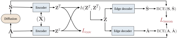
Figure 1: General model architecture. Based upon the input adjacency matrix ${\mathbf{A}}$, we get the diffusion matrix ${\mathbf{S}}$, which needs to be computed only once. The encoder yields the low dimensional projection matrices ${\mathbf{Z}}^{{\mathcal{I}}}$ and ${\mathbf{Z}}^{\overline{{\mathcal{I}}}}$ corresponding to ${\mathcal{I}}$ and $\overline{{\mathcal{I}}}$ respectively. Using a fusion function $h(\cdot)$, The projections ${\mathbf{Z}}^{{\mathcal{I}}}$ and ${\mathbf{Z}}^{\overline{{\mathcal{I}}}}$ are fused into a single projection ${\mathbf{Z}}$, which is then fed to the edge decoder to reconstruct $\mathbf{\hat{A}}$ and $\mathbf{\hat{S}}$.

3.1 Problem Formulation

Suppose an undirected graph ${\mathcal{G}}=({\mathcal{V}},{\mathcal{E}})$ with the adjacency matrix ${\mathbf{A}}\in\{0,1\}^{N\times N}$ and optionally a matrix ${\mathbf{X}}\in{\mathbb{R}}^{N\times F}$ of $F$-dimensional node features, $N$ being the number of nodes. In addition, we construct a diffused version of ${\mathcal{G}}$ by building a diffusion matrix ${\mathbf{S}}\in{\mathbb{R}}^{N\times N}$ from ${\mathbf{A}}$. For brevity we use ${\mathcal{I}}=({\mathbf{A}},{\mathbf{X}})$ and $\overline{{\mathcal{I}}}=({\mathbf{S}},{\mathbf{X}})$ if features are available, otherwise ${\mathcal{I}}={\mathbf{A}}$ and $\overline{{\mathcal{I}}}={\mathbf{S}}$. Given $d$ as the embedding-dimension size, we aim to optimize the model parameters for finding the network embeddings ${\mathbf{Z}}^{{\mathcal{I}}}\in{\mathbb{R}}^{N\times d}$ and ${\mathbf{Z}}^{\overline{{\mathcal{I}}}}\in{\mathbb{R}}^{N\times d}$ from ${\mathcal{I}}$ and $\overline{{\mathcal{I}}}$ such that:

1. ${\mathbf{Z}}^{{\mathcal{I}}}$ and ${\mathbf{Z}}^{\overline{{\mathcal{I}}}}$ can be fused in a way that both ${\mathbf{A}}$ and ${\mathbf{S}}$ can be reconstructed from the fused embedding ${\mathbf{Z}}\in{\mathbb{R}}^{N\times d}$. This allows the embedding to capture the local information from ${\mathcal{I}}$ as well as the information in a larger neighborhood from $\overline{{\mathcal{I}}}$.

2. Same components of different projections have high covariance and vice versa for different components. This adds to the stability towards distortions and also reduces redundancy between different components of the embedding.

Mathematically, the above objective is achieved by minimizing the following loss function

$$L=L_{\mathrm{recon}}+\beta L_{\mathrm{cov}}$$ (1)

where $\beta$ is a hyperparameter of the algorithm to weigh between the reconstruction loss and the cross-covariance loss. The general model architecture is given in figure 1. We first define the loss terms and then brief the modules of the architecture.

3.2 Loss Terms

3.2.1 Reconstruction Loss ($L_{\mathrm{recon}}$)

We aim to learn the model parameters in order to maximize the log probability of recovering both ${\mathbf{A}}$ and ${\mathbf{S}}$ from ${\mathbf{Z}}$. This probability can be written as a marginalization over the joint distribution containing the latent variables ${\mathbf{Z}}$ as

$$\log\Big{(}p({\mathbf{A}},{\mathbf{S}})\Big{)} =\log\Big{(}\int p({\mathbf{A}},{\mathbf{S}},{\mathbf{Z}})d{\mathbf{Z}}\Big{)}$$ (2)

$$=\log\Big{(}\int p({\mathbf{Z}})p({\mathbf{A}}|{\mathbf{Z}})p({\mathbf{S}}|{\mathbf{Z}})d{\mathbf{Z}}\Big{)},$$ (3)

where the prior $p({\mathbf{Z}})$ is modelled as a unit gaussian. Equation 3 assumes conditional independence between ${\mathbf{A}}$ and ${\mathbf{S}}$ given ${\mathbf{Z}}$.

To ensure tractability, we introduce the approximate posterior $q({\mathbf{Z}}|{\mathcal{I}},\overline{{\mathcal{I}}})$ given by

$$q({\mathbf{Z}}|{\mathcal{I}},\overline{{\mathcal{I}}}) =q({\mathbf{Z}}^{{\mathcal{I}}}{\mathbf{Z}}^{\overline{{\mathcal{I}}}}|{\mathcal{I}},\overline{{\mathcal{I}}})$$ (4)

$$=q({\mathbf{Z}}^{{\mathcal{I}}}|{\mathcal{I}})q({\mathbf{Z}}^{\overline{{\mathcal{I}}}}|\overline{{\mathcal{I}}}),$$ (5)

where equation 5 follows from equation 4 because of the assumed conditional independence of ${\mathbf{Z}}^{{\mathcal{I}}}$ and ${\mathbf{Z}}^{\overline{{\mathcal{I}}}}$ given their respective inputs. Both $q({\mathbf{Z}}^{{\mathcal{I}}}|{\mathcal{I}})$ and $q({\mathbf{Z}}^{\overline{{\mathcal{I}}}}|\overline{{\mathcal{I}}})$ are modelled as Gaussians by a single encoder block that learns the parameters $\mu(\cdot)$ and $\sigma(\cdot)$ of the distribution conditioned on the given inputs ${\mathcal{I}}$ and $\overline{{\mathcal{I}}}$ respectively. The term $L_{\mathrm{recon}}$ can now be considered as a negative of the ELBO bound derived as

$$\log\big{(}p({\mathbf{A}},{\mathbf{S}})\big{)} \geq -D_{KL}\Big{(}q({\mathbf{Z}}^{{\mathcal{I}}}|{\mathcal{I}})\ ||\ {\mathcal{N}}(\mathbf{0},{\mathbf{I}})\Big{)}$$

$$-D_{KL}\Big{(}q({\mathbf{Z}}^{\overline{{\mathcal{I}}}}|\overline{{\mathcal{I}}})\ ||\ {\mathcal{N}}(\mathbf{0},{\mathbf{I}})\Big{)}$$

$$-\mathrm{BCE}\big{(}\mathbf{\hat{A}},{\mathbf{A}}\big{)}-\mathrm{BCE}\big{(}\mathbf{\hat{S}},{\mathbf{S}}\big{)}$$ (6)

$$= {\mathcal{L}}_{\mathrm{ELBO}}$$ (7)

$$= -L_{\mathrm{recon}},$$ (8)

where $D_{KL}$ refers to the KL divergence, BCE is the binary cross-entropy, and the matrices $\mathbf{\hat{A}}$ and $\mathbf{\hat{S}}$ refer to reconstructed versions of ${\mathbf{A}}$ and ${\mathbf{S}}$ respectively. The inequality in 6 follows from Jensen’s inequality. It is worth noticing that BCE is computed based upon the edges constructed from the fused embedding ${\mathbf{Z}}$. For detailed derivation, we refer the reader to the supplementary material.

The reconstruction loss in 8 refers to the variational variant BVGAE. For the non-variational case of BGAE, the KL divergence terms get dropped, leaving only the two BCE terms.

3.2.2 Covariance Loss ($L_{\mathrm{cov}}$)

The correlation-loss in [60] (also employed in [5]) involves normalization by the standard deviation of the embedding vectors, centered across the input batch (equation $2$ in [60]). While this works for images and for nodes of the graphs, it has a tendency to obscure the information in the relative strengths of the links in a graph. For graph-datasets, we often replace cosine similarity with dot products, followed by a sigmoid (as done in  [26], [22],and [17], etc.) as it helps in preventing the information in the magnitude of the vectors. Following this approach, instead of computing the cross-correlation matrix, we compute the cross-covariance matrix and use the $\mathrm{sigmoid}$ function to individually normalize the absolute entries $c_{\ell m}$. The loss $L_{\mathrm{cov}}$ is then computed as a summation of two terms corresponding to the mean of diagonal elements and off-diagonal elements of ${\mathcal{C}}$.

$$L_{\mathrm{cov}}= -\frac{1}{N}\sum\limits_{\ell=m}\mathrm{log}(c_{mm})$$

$$-\frac{\lambda}{N(N-1)}\sum\limits_{\ell\neq m}\mathrm{log}(1-c_{\ell m}),$$ (9)

where $\lambda$ defines the trade-off between the two terms. The first term of equation 9 is the invariance term. When minimized, it makes the embedding stable towards distortions. The second term refers to the cross-covariance between different components of ${\mathcal{C}}$. When minimized, it reduces the redundancy between different components of the vectors. The entries $c_{\ell m}$ of ${\mathcal{C}}$ are given by

$$c_{\ell m}=\mathrm{sigmoid}\Big{(}\big{|}\sum\limits_{b=1}^{|{\mathcal{B}}|}(z_{b\ell}^{{\mathcal{I}}}-\overline{z}_{\ell}^{{\mathcal{I}}})(z_{bm}^{\overline{{\mathcal{I}}}}-\overline{z}_{m}^{\overline{{\mathcal{I}}}})\big{|}\Big{)},$$ (10)

where $b$ indexes the batch ${\mathcal{B}}$ with size $|{\mathcal{B}}|$ and the $\ell$-th component of the latent embedding ${\mathbf{z}}^{{\mathcal{I}}}_{b}$ is denoted by $z_{b\ell}^{{\mathcal{I}}}$. The empirical means across embeddings ${\mathbf{Z}}^{{\mathcal{I}}}$ and ${\mathbf{Z}}^{\overline{{\mathcal{I}}}}$ are denoted by $\overline{z}^{{\mathcal{I}}}$ and $\overline{z}^{\overline{{\mathcal{I}}}}$ respectively. It is also worth noticing that the underlying objective is the same for equation 9 as well as the original correlation-based loss in Barlow Twins i.e., ${\mathcal{C}}$ should be as close to identity matrix as possible.

3.3 Model Architecture Blocks

We now describe the modules leading to the loss terms in equation 1 as shown in figure 1.

3.3.1 Diffusion:

The generalized diffusion to construct ${\mathbf{S}}$ from ${\mathbf{A}}$ is given by

$${\mathbf{S}}=\sum\limits_{k=0}^{\infty}\theta_{k}{\mathbf{T}}^{k},$$ (11)

where ${\mathbf{T}}$ is the generalized transition matrix and $\theta_{k}$ are the weighting coefficients. There can be multiple possibilities for $\theta_{k}$ and ${\mathbf{T}}^{k}$ while ensuring the convergence of equation 11 such as the ones proposed in [19], [54], and [27] etc. In this work, we report the case of Personalized PageRank (PPR: [35]) as it consistently gives better results with BGAE/BVGAE. For the detailed results including the Heat Kernel [27], we refer the reader to the supplementary material.

PPR kernel corresponds to ${\mathbf{T}}={\mathbf{A}}{\mathbf{D}}^{-1}$ and $\theta_{k}=\alpha(1-\alpha)^{k}$, where ${\mathbf{D}}$ is the degree matrix and $\alpha\in(0,1)$ is the teleport probability. The corresponding symmetric transition matrix is given by ${\mathbf{T}}={\mathbf{D}}^{-1/2}{\mathbf{A}}{\mathbf{D}}^{-1/2}$. Substitution of ${\mathbf{T}}$ and $\theta_{k}$ into equation 11 leads to a closed form solution for diffusion using PPR kernel as

$${\mathbf{S}}=\alpha\Big{(}{\mathbf{I}}-(1-\alpha){\mathbf{D}}^{-1/2}{\mathbf{A}}{\mathbf{D}}^{-1/2}\Big{)}^{-1}.$$ (12)

Equation 12 restricts the use of PPR-based diffusion for large graphs. However, in practice, there exist multiple approaches to efficiently approximate equation 12 such as the ones proposed by [1] and [51]. In all the results reported in this paper, we use the approximate version of equation 12. Diffusion works well for graphs with high homophily. So BGAE/BVGAE also target similar networks.

3.3.2 Encoder:

This module is responsible for projecting the information in ${\mathcal{I}}$ and $\overline{{\mathcal{I}}}$ into $d$-dimensional embeddings ${\mathbf{Z}}^{{\mathcal{I}}}$ and ${\mathbf{Z}}^{\overline{{\mathcal{I}}}}$ respectively. Following [60], we use a single encoder to encode both versions of the input graph. Our framework is general in the sense that any reasonable encoder can be plugged in to get the learnable projections.

In our work, we have considered two options for the encoder block, consequently leading to two variants of the framework.

• For BGAE, we use a single layer GCN encoder.

• For BVGAE, we employ a simple variational encoder that learns the parameters $\mu(\cdot)$ and $\sigma(\cdot)$ of a gaussian distribution conditioned upon the input samples. The latent samples can then be generated by following the reparameterization trick [24].

3.3.3 Fusion Function:

The function $h(\cdot)$ is used to fuse ${\mathbf{Z}}^{{\mathcal{I}}}$ and ${\mathbf{Z}}^{\overline{{\mathcal{I}}}}$ into a single matrix ${\mathbf{Z}}$. In this work we define ${\mathbf{Z}}$ as a weighted sum of ${\mathbf{Z}}^{{\mathcal{I}}}$ and ${\mathbf{Z}}^{\overline{{\mathcal{I}}}}$ as

$$h({\mathbf{z}}_{i}^{{\mathcal{I}}},{\mathbf{z}}_{i}^{\overline{{\mathcal{I}}}})=\phi_{i}^{{\mathcal{I}}}{\mathbf{z}}_{i}^{{\mathcal{I}}}+\phi_{i}^{\overline{{\mathcal{I}}}}{\mathbf{z}}_{i}^{\overline{{\mathcal{I}}}},$$ (13)

where the weights $\{\phi_{i}^{{\mathcal{I}}}\}_{i=1}^{N}$ and $\{\phi_{i}^{\overline{{\mathcal{I}}}}\}_{i=1}^{N}$ can either be fixed or learned. In this work we report two variants of the fusion function.

• Fixing $\phi_{i}^{{\mathcal{I}}}=\phi_{i}^{\overline{{\mathcal{I}}}}=0.5\ \forall i$.

• Learning $\{\phi_{i}^{{\mathcal{I}}}\}_{i=1}^{N}$ and $\{\phi_{i}^{\overline{{\mathcal{I}}}}\}_{i=1}^{N}$ using attention mechanism.

For attention, we compute the dot products of different embeddings of the same node with respective learnable weight vectors, followed by LeakyReLU activation. Afterwards a $\mathrm{softmax}$ is applied to get the probabilistic weight assignments, i.e.

$$\phi_{i}^{{\mathcal{I}}} =\frac{\exp\Big{(}\mathrm{A}\big{(}{\mathbf{w}}_{1}^{T}{\mathbf{z}}_{i}^{{\mathcal{I}}}\big{)}\Big{)}}{\exp\Big{(}\mathrm{A}\big{(}{\mathbf{w}}_{1}^{T}{\mathbf{z}}_{i}^{{\mathcal{I}}}\big{)}\Big{)}+\exp\Big{(}\mathrm{A}\big{(}{\mathbf{w}}_{2}^{T}{\mathbf{z}}_{i}^{\overline{{\mathcal{I}}}}\big{)}\Big{)}},$$ (14)

$$\phi_{i}^{\overline{{\mathcal{I}}}} =1-\phi_{i}^{{\mathcal{I}}}.$$ (15)

where $\textrm{A}(\cdot)$ is the LeakyReLU activation function and ${\mathbf{w}}_{1},{\mathbf{w}}_{2}\in{\mathbb{R}}^{d}$ are learnable weight vectors.

3.3.4 Decoder

Since our approach is auto-encoder-based, we use the edge decoder as proposed by [26], to reconstruct the entries $\hat{a}_{ij}$ of $\mathbf{\hat{A}}$ as

$$\hat{a}_{ij}=\sigma({\mathbf{z}}_{i}^{T}{\mathbf{z}}_{j})$$ (16)

The entries of $\mathbf{\hat{S}}$ can also be reconstructed in similar fashion.

4 Experiments

This section describes the datasets and the experiments conducted to evaluate the efficacy of our approach. We choose eight benchmark datasets including Wikipedia articles (WikiCS) [32], Amazon co-purchase data networks (AmazonPhoto and AmazonComputers [30]), extracts from Microsoft Academic Graph (CoauthorCS and CoauthorPhysics) [43], and citation networks (Cora, CiteSeer and PubMed) [42]. The basic characteristics of these datasets are briefed in table 1. We first report the results for link prediction. The network embedding learned by BGAE and BVGAE is unsupervised as no node labels are used during training. Hence, to measure the quality of the network embedding, we analyze our approach for two downstream tasks: clustering and transductive node classification. For the interested readers, the supplementary material contains a detailed analysis of BGAE and BVGAE in different settings. We use the AWS EC2 instance type g4dn.4xlarge with $16$GB GPU for training. For reproducibility, the implementation details of all the experiments along with the code are provided in [2]. For all the experiments, we report publicly available results from our competitors.

Table 1: Datasets used for evaluation.

Dataset	Nodes	Edges	Features	Classes
Cora [42]	2,708	5,297	1,433	7
CiteSeer [42]	3,312	4,732	3,703	6
PubMed [42]	19,717	44,338	500	3
WikiCS [32]	11,701	216,123	300	10
AmazonComputers [30]	13,752	245,861	767	10
AmazonPhotos [30]	7,650	119,081	745	8
CoauthorCS [43]	18,333	81,894	6,805	15
CoauthorPhysics [43]	34,493	247,962	8,415	5

4.1 Link Prediction

Table 2: Link prediction performance, as evaluated by AUC and AP metrics. The best results are styled as bold and second best are underlined.

Algorithm	Cora		CiteSeer		PubMed		CoauthorCS		AmazonPhoto
	AUC	AP	AUC	AP	AUC	AP	AUC	AP	AUC	AP
DeepWalk	83.10	85.00	80.50	83.60	84.40	84.10	91.74	91.19	91.48	90.79
GAE	91.00	92.00	89.50	89.90	96.40	96.50	94.09	93.86	93.86	92.96
VGAE	91.40	92.60	90.80	92.00	94.40	94.70	89.60	89.36	92.05	92.02
ARGA	92.40	93.20	91.90	93.00	96.80	97.10	91.99	92.54	96.10	95.40
ARVGA	92.40	92.60	92.40	93.00	96.50	96.80	93.32	93.32	92.70	90.90
GALA	92.10	92.20	94.40	94.80	91.50	89.70	93.81	94.49	91.80	91.00
DGI	89.80	89.70	95.50	95.70	91.20	92.20	94.87	94.34	92.24	92.14
GIC	93.50	93.30	97.00	96.80	93.70	93.50	95.03	94.94	92.70	92.34
GMI	95.10	95.60	97.80	97.40	96.37	96.04	96.37	95.04	93.88	92.67
GCA	95.75	95.47	96.44	96.49	95.28	95.52	96.31	96.28	93.25	92.74
MVGRL	90.52	90.45	92.89	92.89	92.45	92.17	95.17	95.58	92.89	92.45
G-BT	87.46	86.84	93.42	93.01	94.53	94.26	92.64	91.40	95.12	95.45
BGAE	98.52	98.42	98.59	98.61	97.78	97.68	96.31	95.44	95.01	94.24
BGAE + Att	98.79	98.73	98.56	98.57	98.06	98.03	96.51	95.65	95.18	94.49
BVGAE	97.87	97.62	98.63	98.57	97.93	97.89	96.12	95.13	94.61	94.29
BVGAE + Att	98.03	97.77	98.23	98.08	97.77	97.74	96.21	95.34	94.97	94.28

4.1.1 Comparison Methods

For link prediction, we select 12 competitors. We start with DeepWalk [38] as the baseline.

Auto-encoder based Architectures: We include graph auto-encoder or GAE which aims to reconstruct the adjacency matrix for the input graph. The variational graph auto-encoder or VGAE [26] is its variational counterpart that extends the idea of variational auto-encoder or VAE [24] to graph domain. In the case of adversarially regularized graph auto-encoder or ARGA [36], the latent representation is forced to match the prior via an adversarial training scheme. Just like VGAE, there exists a variational alternative to ARGA, known as adversarially regularized variational graph auto-encoder or ARVGA. GALA [37] learns network embedding by treating encoding and decoding steps as Laplacian smoothing and Laplace sharpening respectively.

Contrastive Methods: DGI [48] leverages Deep-Infomax [18] for graph datasets. Graph InfoClust or GIC [29] learns network embedding by maximizing the mutual information with respect to the graph-level summary as well as the cluster-level summaries. GMI [28] aims to learn node representations while aiming to improve generalization performance via added contrastive regularization. GCA [65] proposes adaptive augmentation techniques to contrast views between nodes and subgraphs or structurally transformed graphs. MVGRL [17] learns graph embedding by contrasting multiple views of the input data.

In addition, we include G-BT [5] which is another approach making use of the redundancy-minimization principle introduced in [60] as discussed in section 2.2.

For link prediction, we skip the three datasets where many public results are missing and report these partial results in the supplementary material.

4.1.2 Settings

For link prediction, we follow the same link split as adopted by our competitors, i.e., we split the edges into the training, validation, and test sets containing 85%, 5%, and 10% links respectively. For all the competitors we keep the same settings as given by the authors. For the methods where multiple variants are given by the authors(e.g., ARGA, ARVGA, etc.), we report the best results amongst all the variants. For our approach, we keep the latent dimension to $512$ for all the experiments except CoauthorPhysics where $d=128$ to avoid out-of-memory issues. We use a single layer GCN encoder for BGAE, and two GCN encoders to output the parameters $\mu(\cdot)$ and $\sigma(\cdot)$ in case of the variational encoder block of BVGAE. For all the experiments, we get ${\mathbf{S}}$ by setting the average degree to $25$. The value of the hyperparameter $\lambda$ in equation 9 is set to $5e^{-3}$ for all the experiments. This is the same as proposed in Barlow-Twins[60]. Adam [23] is used as the optimizer with learning rate and rate decay set to 0.01 and $5e^{-6}$. The hyperparameter $\beta$ is fixed to $1$ for all experiments. Instead of computing a closed-form solution, it is sufficient to compute the BCE loss using the samples ${\mathbf{z}}$. For this, we follow other auto-encoder-based approaches such as [26, 22] for dataset splits and sampling of positive/negative edges for every training iteration. For evaluation, we report the area under the curve (AUC) and average precision (AP) metrics. All the results are the average of 10 runs. Further implementation details can be found in [2].

Table 3: Transductive node classification performance, as evaluated by accuracy. The best results are styled as bold and second best are underlined. OOM refers to Out-of-Memory.

Algorithm	Cora	CiteSeer	PubMed	WikiCS	CoauthorCS	CoauthorPhysics	AmazonComputers	AmazonPhoto
Raw	47.87	49.33	69.11	71.98	90.37	93.58	73.81	78.53
DeepWalk	70.66	51.39	74.31	77.21	87.70	94.90	86.28	90.05
GAE	71.53	65.77	72.14	70.15	90.01	94.92	85.18	91.68
VGAE	75.24	69.05	75.29	75.63	92.11	94.52	86.44	92.24
ARGA	74.14	64.14	74.12	66.88	89.41	93.10	84.39	92.68
ARVGA	74.38	64.24	74.69	67.37	88.54	94.30	84.66	92.49
DGI	81.68	71.47	77.27	75.35	92.15	94.51	83.95	91.61
GIC	81.73	71.93	77.33	77.28	89.40	93.10	84.89	92.11
GRACE	80.04	71.68	79.53	80.14	92.51	94.70	87.46	92.15
GMI	83.05	73.03	80.10	74.85	OOM	OOM	82.21	90.68
GCA	82.10	71.30	80.20	78.23	92.95	95.73	88.94	92.53
MVGRL	82.90	72.60	79.40	77.52	92.11	92.11	87.52	91.74
BGRL	82.70	71.10	79.60	79.98	93.31	95.56	89.68	92.87
G-BT	80.80	73.00	80.00	76.65	92.95	95.07	88.14	92.63
BGAE	83.51	72.43	81.84	78.93	93.76	95.01	92.24	91.10
BGAE + Att	83.60	72.41	80.95	79.53	93.76	95.64	92.44	91.89
BVGAE	82.62	72.97	80.02	77.52	93.25	95.13	89.19	89.38
BVGAE + Att	82.57	73.09	80.25	77.82	93.15	95.60	89.91	89.98

4.1.3 Results

Table 2 gives the results for the link prediction task. For our approach, we give the results for BGAE as well as BVGAE, both with and without attention. We can observe that our approach achieves the best or second best results in all the datasets. Overall the variant of BGAE with attention performs well across all the datasets and metrics. This validates the choice of attention as a fusion function. Among the competitors, the contrastive approaches perform relatively better across all the datasets. One exception is AmazonPhoto where ARGA achieves the best results. However, as the next sections demonstrate, the performance of ARGA/ARVGA degrades for downstream node classification and clustering. Another thing to note is the results of G-BT. As the training epochs go on for G-BT, the results degrade rapidly, often by about 30% of the results reported in table 2. Apart from AmazonPhotos, there is a healthy margin between BGAE and G-BT mainly because unlike BGAE, G-BT does not explicitly preserve the information in the links.

4.2 Transductive Node Classification

4.2.1 Comparison Methods

We compare with 14 competitors for transductive node classification, using raw features and DeepWalk(with features) as the baselines. In addition to the methods briefed in section 4.1.1, we include two more contrastive methods i.e. GRACE and BGRL: GRACE [64] learns network embedding by making use of multiple views and contrasting the representation of a node with its raw information (e.g., node features) or neighbors’ representations in different views. BGRL [45] eliminates the need for negative samples by minimizing invariance between two augmented versions of mini-batches of graphs.

4.2.2 Settings

The training phase uses the same settings as reported in section 4.1.2. For transductive node classification, we do not need to split the edges into training/validation/test sets. So we use all the edges for self-supervised learning of the node embeddings. For evaluating the embedding, a logistic regression head is used with lbfgs solver. For this, we use the default settings of the scikit-learn package. For citation datasets (Cora, CiteSeer, and PubMed), we follow the standard public splits for training/validation/test sets used in many previous works such as [58, 48, 21, 25], i.e., 20 labels per class for training, 500 samples for validation, and 1000 for testing. For WikiCS, we average over the 20 splits that are publicly provided. For the rest of the datasets (AmazonPhoto, AmazonComputers, CoauthorPhysics, and coauthorCS), we follow the split configuration of B-JT, i.e. generate random splits with training, validation, and test sets containing 10%, 10%, and 80% nodes respectively. For evaluation, we use accuracy as the metric.

4.2.3 Results

Table 3 gives the comparison between different algorithms for transductive node classification. We can again observe consistently good results by our approach for all eight datasets. For this task, the margin is rather small, especially for Cora and CiteSeer, compared to the best competitor i.e. GMI. Nonetheless, our point still stands well-conveyed that our approach performs on par with the well-known network embedding techniques for transductive node classification. A comparison of table 3 with table 2 demonstrates inconsistencies in the performance of our competitors for the two tasks. This is mainly because either the competitors do not explicitly preserve information in the links (e.g. MVGRL, G-BT, etc), or link prediction is their main focus (e.g., in GAE/ARGA, etc). For instance, ARGA performed reasonably well for link prediction, but fails to give a similar consistent performance across all datasets in table 3. On the other hand, MVGRL performs well in table 3, although its performance suffered in table 2.

4.3 Node Clustering

Table 4: Node clustering performance, as evaluated by NMI. The best results are styled as bold and second best are underlined. OOM refers to Out-of-Memory.

Algorithm	Cora	CiteSeer	PubMed	WikiCS	CoauthorCS	CoauthorPhysics	AmazonComputers	Amazon-Photos
K-means	32.10	30.50	0.10	18.20	64.20	48.90	16.60	28.20
GAE	42.90	17.60	27.70	24.30	73.10	54.50	44.10	61.60
VGAE	43.60	15.60	22.90	26.10	73.30	56.30	42.30	53.00
ARGA	44.90	35.00	30.50	27.50	66.80	51.20	23.50	57.70
ARVGA	52.60	33.80	29.00	28.70	61.60	52.60	23.70	45.50
DGI	41.10	31.50	27.70	31.00	74.70	67.00	31.80	37.60
GRACE	46.18	38.29	16.27	42.82	75.62	OOM	47.93	65.13
GCA	55.70	37.40	28.90	29.90	73.50	59.40	42.60	34.40
MVGRL	60.90	44.00	31.50	26.30	74.00	59.40	24.40	34.40
G-BT	43.40	41.57	29.52	27.46	74.37	59.8	65.55	52.39
BGAE	62.42	43.36	38.46	45.80	80.10	68.01	66.98	67.13
BGAE + Att	62.27	43.84	38.59	46.93	80.30	68.12	66.93	67.43
BVGAE	59.60	43.29	37.41	40.78	79.01	67.10	60.98	61.33
BVGAE + Att	59.82	43.27	37.47	40.86	79.42	67.06	61.44	61.62

4.3.1 Settings

For clustering, we choose 10 methods in total for comparison, with the baseline established by K-Means. The experimental configuration for node clustering follows the same pattern as in section 4.1.2. For clustering, we use all the edges just like in section 4.2.2, i.e., all the edges are used for self-supervised learning of the node-embeddings. Afterward, we use K-Means to infer the cluster assignments from the embeddings. For evaluation, we use normalized mutual information (NMI) as the metric.

4.3.2 Results

The results of the experiments for downstream node clustering are given in table 4. Here again, we perform consistently well for all the datasets except CiteSeer, where we achieve the second-best results by a small margin. It is worth noticing that apart from CiteSeer, we achieve both the best and the second results using different variants of BGAE. A comparison of table 4 with table 2 and table 3 again highlights that no competitor algorithm performs consistently well for all the tasks and datasets. For instance, ARGA performed well on some datasets in table 2. However, its performance suffers in table 4. Similarly, GMI, which performs well in table 3, is outperformed by many other algorithms in node clustering. On the other hand, the algorithms such as GIC, that perform well in table 4 are outperformed by others in table 3. This highlights the task-specific nature of the network embedding learned by different competitors and also shows the efficacy of BGAE across multiple tasks and datasets.

5 Conclusion

This work proposes a simple yet effective auto-encoder based approach for network embedding that simultaneously employs the information in the immediate and larger neighborhoods. To construct a uniform network embedding, the two information sources are efficiently coupled using the redundancy-minimization principle. We propose two variants, BGAE and BVGAE, depending upon the type of encoder block. To construct larger neighborhood from the immediate neighborhood, we use graph-diffusion. Our work is restricted to the networks with high homophily, because diffusion only works well for such networks. As demonstrated by the extensive experimentation, our approach is on par with the well-known baselines, often outperforming them over a variety of tasks such as link prediction, clustering, and transductive node classification.

SUPPLEMENTARY MATERIAL

Throughout the supplementary material, we follow the notation and references from the main paper.

6 DERIVATION OF $L_{\mathrm{recon}}$ FOR VARIATIONAL CASE

As mentioned in the paper, we aim to learn the model parameters $\theta$ to maximize the log probability of recovering the joint probability of ${\mathbf{A}}$ and ${\mathbf{S}}$ from ${\mathbf{Z}}$, given as

$$\log\Big{(}p({\mathbf{A}},{\mathbf{S}})\Big{)} =\log\Big{(}\int p({\mathbf{A}},{\mathbf{S}},{\mathbf{Z}})d{\mathbf{Z}}\Big{)}$$ (17)

$$=\log\Big{(}\int p({\mathbf{Z}})p({\mathbf{A}}|{\mathbf{Z}})p({\mathbf{S}}|{\mathbf{Z}})d{\mathbf{Z}}\Big{)}.$$ (18)

Here we assume conditional independence between ${\mathbf{A}}$ and ${\mathbf{S}}$ given ${\mathbf{Z}}$. The approximate posterior, introduced for tractability, is given as

$$q({\mathbf{Z}}|{\mathcal{I}},\overline{{\mathcal{I}}}) =q({\mathbf{Z}}^{{\mathcal{I}}}{\mathbf{Z}}^{\overline{{\mathcal{I}}}}|{\mathcal{I}},\overline{{\mathcal{I}}})$$ (19)

$$=q({\mathbf{Z}}^{{\mathcal{I}}}|{\mathcal{I}})q({\mathbf{Z}}^{\overline{{\mathcal{I}}}}|{\mathcal{I}},{\mathbf{Z}}^{{\mathcal{I}}})$$ (20)

$$=q({\mathbf{Z}}^{{\mathcal{I}}}|{\mathcal{I}})q({\mathbf{Z}}^{\overline{{\mathcal{I}}}}|\overline{{\mathcal{I}}}),$$ (21)

where equation 21 follows from equation 20 because of the assumed conditional independence of ${\mathbf{Z}}^{{\mathcal{I}}}$ and ${\mathbf{Z}}^{\overline{{\mathcal{I}}}}$ given their respective inputs ${\mathcal{I}}$ and $\overline{{\mathcal{I}}}$. The corresponding prior $p({\mathbf{Z}})$ is assumed as a joint of i.i.d. Gaussians, i.e.

$$p({\mathbf{Z}})=p({\mathbf{Z}}^{{\mathcal{I}}})p({\mathbf{Z}}^{\overline{{\mathcal{I}}}})={\mathcal{N}}(\mathbf{0},{\mathbf{I}}){\mathcal{N}}(\mathbf{0},{\mathbf{I}}).$$ (22)

So $L_{\mathrm{recon}}$ can now be considered as a negative of the ELBO bound derived as

$$\log\big{(}p({\mathbf{A}},{\mathbf{S}})\big{)} = \log\Big{(}\int p({\mathbf{Z}})p({\mathbf{A}}|{\mathbf{Z}})p({\mathbf{S}}|{\mathbf{Z}})d{\mathbf{Z}}\Big{)}$$ (23)

$$= \log\Big{(}\int\frac{p({\mathbf{Z}})p({\mathbf{A}}|{\mathbf{Z}})p({\mathbf{S}}|{\mathbf{Z}})}{q({\mathbf{Z}}|{\mathcal{I}},\overline{{\mathcal{I}}})}q({\mathbf{Z}}|{\mathcal{I}},\overline{{\mathcal{I}}})d{\mathbf{Z}}\Big{)}$$ (24)

$$= \log\Bigg{(}{\mathbb{E}}_{{\mathbf{Z}}\sim q}\Big{\{}\frac{p({\mathbf{Z}})p({\mathbf{A}}|{\mathbf{Z}})p({\mathbf{S}}|{\mathbf{Z}})}{q({\mathbf{Z}}|{\mathcal{I}},\overline{{\mathcal{I}}})}\Big{\}}\Bigg{)}$$ (25)

$$\geq {\mathbb{E}}_{{\mathbf{Z}}\sim q}\Bigg{\{}\log\Big{(}\frac{p({\mathbf{Z}})p({\mathbf{A}}|{\mathbf{Z}})p({\mathbf{S}}|{\mathbf{Z}})}{q({\mathbf{Z}}|{\mathcal{I}},\overline{{\mathcal{I}}})}\Big{)}\Bigg{\}},$$ (26)

where (26) follows from Jensen’s Inequality. Using the factorizations in equation 20 and equation 21, we can now separate the factors inside $\log$ of (26) as

$${\mathbb{E}}_{{\mathbf{Z}}\sim q}\Bigg{\{}\log\Big{(}\frac{p({\mathbf{Z}})p({\mathbf{A}}|{\mathbf{Z}})p({\mathbf{S}}|{\mathbf{Z}})}{q({\mathbf{Z}}|{\mathcal{I}},\overline{{\mathcal{I}}})}\Big{)}\Bigg{\}}$$

$$={\mathbb{E}}_{{\mathbf{Z}}\sim q}\Bigg{\{}\log\Big{(}\frac{p({\mathbf{Z}}^{{\mathcal{I}}})p({\mathbf{Z}}^{\overline{{\mathcal{I}}}})p({\mathbf{A}}|{\mathbf{Z}})p({\mathbf{S}}|{\mathbf{Z}})}{q({\mathbf{Z}}^{{\mathcal{I}}}|{\mathcal{I}})q({\mathbf{Z}}^{\overline{{\mathcal{I}}}}|\overline{{\mathcal{I}}})}\Big{)}\Bigg{\}}$$ (27)

$$={\mathbb{E}}_{{\mathbf{Z}}\sim q}\Bigg{\{}\log\Big{(}\frac{p({\mathbf{Z}}^{{\mathcal{I}}})}{q({\mathbf{Z}}^{{\mathcal{I}}}|{\mathcal{I}})}\Big{)}+\log\Big{(}\frac{p({\mathbf{Z}}^{\overline{{\mathcal{I}}}})}{q({\mathbf{Z}}^{\overline{{\mathcal{I}}}}|\overline{{\mathcal{I}}})}\Big{)}$$

$$\quad\quad\quad\quad\quad+\log\Big{(}p({\mathbf{A}}|{\mathbf{Z}})\Big{)}+\log\Big{(}p({\mathbf{S}}|{\mathbf{Z}})\Big{)}\Bigg{\}}$$ (28)

$$=-D_{KL}\Big{(}q({\mathbf{Z}}^{{\mathcal{I}}}|{\mathcal{I}})||p({\mathbf{Z}}^{{\mathcal{I}}})\Big{)}$$

$$\ \ \ \ -D_{KL}\Big{(}q({\mathbf{Z}}^{\overline{{\mathcal{I}}}}|\overline{{\mathcal{I}}})||p({\mathbf{Z}}^{\overline{{\mathcal{I}}}})\Big{)}$$

$$\ \ \ \ -\mathrm{BCE}(\mathbf{\hat{A}},{\mathbf{A}})-\mathrm{BCE}(\mathbf{\hat{S}},{\mathbf{S}})$$ (29)

$$=-D_{KL}\Big{(}q({\mathbf{Z}}^{{\mathcal{I}}}|{\mathcal{I}})||{\mathcal{N}}(\mathbf{0},{\mathbf{I}})\Big{)}$$

$$\ \ \ \ -D_{KL}\Big{(}q({\mathbf{Z}}^{\overline{{\mathcal{I}}}}|\overline{{\mathcal{I}}})||{\mathcal{N}}(\mathbf{0},{\mathbf{I}})\Big{)}$$

$$\ \ \ \ -\mathrm{BCE}(\mathbf{\hat{A}},{\mathbf{A}})-\mathrm{BCE}(\mathbf{\hat{S}},{\mathbf{S}})$$ (30)

$$={\mathcal{L}}_{\mathrm{ELBO}}=-L_{\mathrm{recon}.}$$ (31)

7 Detailed Comparison

We now aggregate the publicly available results for all three tasks discussed in the paper. The publicly available approaches often cover only a subset of the datasets evaluated in this work. So we leave the table cells empty in case of missing public results. In addition to the competitors mentioned in the paper, we add new competitors for different tasks.

Table 5: Link prediction performance, as evaluated by AUC and AP metrics. The best results are styled as bold and second best are underlined.

Algorithm	Cora		CiteSeer		PubMed		WikiCS		CoauthorCS		AmazonComputers		AmazonPhoto
	AUC	AP	AUC	AP	AUC	AP	AUC	AP	AUC	AP	AUC	AP	AUC	AP
Spectral	84.60	88.50	80.50	85.00	84.20	87.80
DeepWalk	83.10	85.00	80.50	83.60	84.40	84.10			91.74	91.19	87.35	91.48	91.48	90.79
GCN	90.47	91.62	82.56	83.20	89.56	90.28
HGCN	92.90	93.45	95.25	95.97	96.30	96.75
GAT	93.17	93.81	86.48	87.51	91.46	92.28
HGAT	94.02	94.63	95.84	95.89	94.18	94.42
GAE	91.00	92.00	89.50	89.90	96.40	96.50	93.00	94.80	94.09	93.86	93.61	93.36	93.86	92.96
VGAE	91.40	92.60	90.80	92.00	94.40	94.70	93.60	95.00	89.60	89.36	93.15	92.40	92.05	92.02
ARGA	92.40	93.20	91.90	93.00	96.80	97.10	93.40	94.70	91.99	92.54			96.10	95.40
ARVGA	92.40	92.60	92.40	93.00	96.50	96.80	94.70	94.80	93.32	93.32			92.70	90.90
DGLFRM	93.43	93.76	93.79	94.38	93.95	94.97
GALA	92.10	92.20	94.40	94.80	91.50	89.70	93.60	93.10	93.81	94.49			91.80	91.00
Graphite	94.70	94.90	97.30	97.40	97.40	97.40
DGI	89.80	89.70	95.50	95.70	91.20	92.20			94.87	94.34			92.24	92.14
GIC	93.50	93.30	97.00	96.80	93.70	93.50			95.03	94.94			92.70	92.34
GMI	95.10	95.60	97.80	97.40	96.37	96.04			96.37	95.04			93.88	92.67
GCA	95.75	95.47	96.44	96.49	95.28	95.52			96.31	96.28			93.25	92.74
MVGRL	90.52	90.45	92.89	92.89	92.45	92.17			95.17	95.58			92.89	92.45
G-BT	87.46	86.84	93.42	93.01	94.53	94.26	93.05	93.18	92.64	91.40	91.54	90.59	95.12	94.45
BGAE	98.52	98.42	98.59	98.61	97.78	97.68	97.23	97.69	96.31	95.44	95.01	94.04	95.01	94.24
BGAE + Att	98.79	98.73	98.56	98.57	98.06	98.03	97.73	98.03	96.51	95.65	95.13	94.48	95.18	94.49
BVGAE	97.87	97.62	98.63	98.57	97.93	97.89	97.62	97.42	96.12	95.13	94.66	94.01	94.61	94.29
BVGAE + Att	98.03	97.77	98.23	98.08	97.77	97.74	97.85	98.05	96.21	95.34	94.90	94.07	94.97	94.28

7.1 Link Prediction

We add the following approaches in addition to the ones given in table 2: GNN based architectures GCN [25] and GAT [47], along with their hyperbolic variants HGCN [9] and HGAT [15]. Deep Generative Latent Feature Relational Model or DGLFRM [31] that aims to reconstruct the adjacency matrix while retaining the interpretability of stochastic block models. Graph InfoClust or GIC [29], which learns network embedding by maximizing the mutual information with respect to the graph-level summary as well as the cluster-level summaries. Graphite [14], which is another auto-encoder based generative model that employs a multi-layer procedure, inspired by low-rank approximations, to iteratively refine the reconstructed graph via message passing.

7.1.1 Results

We can notice that our approach is still either best or second best including all the competitors. GMI and GCA achieve good results for CoauthorCS, Graphite performs consistently well for all the datasets. However these algorithms suffer when evaluated for clustering and transductive node classification.

7.2 Clustering

Table 6: Node clustering performance, as evaluated by NMI. The best results are styled as bold and second best are underlined. OOM refers to Out-of-Memory.

Algorithm	Cora	CiteSeer	PubMed	WikiCS	CoauthorCS	CoauthorPhysics	AmazonComputers	AmazonPhoto
K-means	32.10	30.50	0.10	18.20	64.20	48.90	16.60	28.20
Spectral	12.70	5.60	4.20
DeepWalk	32.70	8.80	27.90
BigClam	0.70	3.60	0.60
DNGR	31.80	18.00	15.50
RMSC	25.50	13.90	25.50
TADW	44.10	29.10	0.10
GAE	42.90	17.60	27.70	24.30	73.10	54.50	44.10	61.60
VGAE	43.60	15.60	22.90	26.10	73.30	56.30	42.30	53.00
ARGA	44.90	35.00	30.50	27.50	66.80	51.20	23.50	57.70
ARVGA	52.60	33.80	29.00	28.70	61.60	52.60	23.70	45.50
GALA	57.70	44.10	32.70					51.20
Graphite	54.12	42.42	32.40
DGI	41.10	31.50	27.70	31.00	74.70	67.00	31.80	37.60
GIC	53.70	45.30	31.90
GRACE	46.18	38.29	16.27	42.82	75.62	OOM	47.93	65.13
AGC	53.70	41.10	31.60
GMI	50.33	38.14	26.20
GMNN	53.72	41.73	31.77
DAEGC	52.80	39.70	26.60
DBGAN	56.00	40.70	32.40					48.50
GCA	55.70	37.40	28.90	29.90	73.50	59.40	42.60	34.40
MVGRL	60.90	44.00	31.50	26.30	74.00	59.40	24.40	34.40
BGRL				39.69	77.32	55.68	53.64	68.41
G-BT	43.40	41.57	29.52	27.46	74.37	59.80	65.55	52.39
BGAE	62.42	43.36	38.46	45.80	80.10	68.01	66.98	67.13
BGAE + Att	62.27	43.84	38.59	46.93	80.30	68.12	66.93	67.43
BVGAE	59.60	43.29	37.41	40.78	79.01	67.10	60.98	61.33
BVGAE + Att	59.82	43.27	37.47	40.86	79.42	67.06	61.44	61.62

We include the following clustering-specific competitors in addition to the ones given in table 4 and section 7.1: BigClam [57] uses matrix factorization for community detection. DNGR [8] learns network embedding by using stacked denoising auto-encoders. RMSC [53] introduces a multi-view spectral clustering approach to recover a low-rank transition probability matrix from the transition matrices corresponding to multiple views of input data. TADW [56] learns the network embedding by treating DeepWalk as matrix factorization and adding the features of vertices. AGC [61] performs attributed graph clustering by first obtaining smooth node feature representations via k-order graph convolution and then performing spectral clustering on the learned features. DAEGC [49] uses GAT to encode the importance of the neighboring nodes in the latent space such that both the reconstruction loss and the KL-divergence based clustering loss are minimized.

In addition, we include some well-known approaches for unsupervised network embedding. DBGAN [62] introduces a bidirectional adversarial learning framework to learn network embedding in such a way that the prior distribution is also estimated along with the adversarial learning. GMI [28] is an unsupervised approach to learn node representations while aiming to improve generalization performance via added contrastive regularization. GMNN [40] relies on a random field model, which can be trained with variational expectation maximization.

7.2.1 Results

Our approach performs the best overall, although GIC and BGRL achieve the best results for CiteSeer and AmazonPhoto respectively. Graphite performed well in table 5, but for clustering, it is outperformed by many other competitors. The converse is true for GIC and GALA, which outperform BGAE for a single dataset in clustering, but fail to compete in the link-prediction task. Similarly, DBGAN emerges as a decent competitor for node-clustering. However, as we will see in the next section, its performance degrades for the task of node classification. We cannot comment on BGRL because we could neither find its public implementation nor any publicly published results for link-prediction on the selected datasets.

7.3 Transductive Node Classification

Table 7: Transductive node classification performance, as evaluated by accuracy. The best results are styled as bold and second best are underlined.

Algorithm	Cora	CiteSeer	PubMed	WikiCS	CoauthorCS	CoauthorPhysics	AmazonComputers	AmazonPhoto
Raw	47.87	49.33	69.11	71.98	90.37	93.58	73.81	78.53
DeepWalk	70.66	51.39	74.31	77.21	87.70	94.90	86.28	90.05
GAE	71.53	65.77	72.14	70.15	90.01	94.92	85.18	91.68
VGAE	75.24	69.05	75.29	75.63	92.11	94.52	86.44	92.24
ARGA	74.14	64.14	74.12	66.88	89.41	93.10	84.39	92.68
ARVGA	74.38	64.24	74.69	67.37	88.54	94.30	84.66	92.49
Graphite	82.10	71.00	79.30
DGI	81.68	71.47	77.27	75.35	92.15	94.51	83.95	91.61
GIC	81.73	71.93	77.33	77.28	89.40	93.10	84.89	92.11
GRACE	80.04	71.68	79.53	80.14	92.51	94.70	87.46	92.15
AGC	70.90	71.89	68.91
GMI	83.05	73.03	80.10	74.85	OOM	OOM	82.21	90.68
GMNN	82.78	71.54	80.60
DBGAN	77.30	69.70	77.50
GCA	82.10	71.30	80.20	78.23	92.95	95.73	88.94	92.53
MVGRL	82.90	72.60	79.40	77.52	92.11	92.11	87.52	91.74
BGRL	82.70	71.10	79.60	79.98	93.31	95.56	89.68	92.87
G-BT	80.80	73.00	80.00	76.65	92.95	95.07	88.14	92.63
BGAE	83.51	72.43	81.84	78.93	93.76	95.01	92.24	91.10
BGAE + Att	83.60	72.41	80.95	79.53	93.76	95.64	92.44	91.89
BVGAE	82.62	72.97	80.02	77.52	93.25	95.13	89.19	89.38
BVGAE + Att	82.57	73.09	80.25	77.82	93.15	95.60	89.91	89.98

The competitors evaluated in table 7 have already been introduced in the main paper and in section 7.1 and section 7.2. We exclude some methods that are specifically designed for clustering, because such methods perform poor on transductive node classification.

7.3.1 Results

GRACE, GMI, GALA, and BGRL perform well for WikiCS, CiteSeer, and AmazonPhoto. However our approach performs the best overall as we achieve the best or second-best results in 6 out of 8 datasets. This demonstrates the efficacy of our approach over a variety of tasks unlike many competitors that shine only in some of the target tasks.

8 Ablation Studies

We now observe how our approach is affected by changes in $\beta$ from equation 1, $\lambda$ from equation 9, and average-node degree used for sparsification of $\overline{{\mathbf{S}}}$ into ${\mathbf{S}}$. For sake of brevity, we only plot the results for transductive node classification task because link prediction and clustering follow a similar pattern. To emphasize the relative performance, the vertical axes correspond to the percentage accuracy scores relative to the ones reported in table 3.

8.1 Effect of $\beta$

To evaluate the effect of $\beta$ in equation 1, we sweep $\beta$ for the values across the set $\{0,0.1,1,10,100,1000,10000\}$.

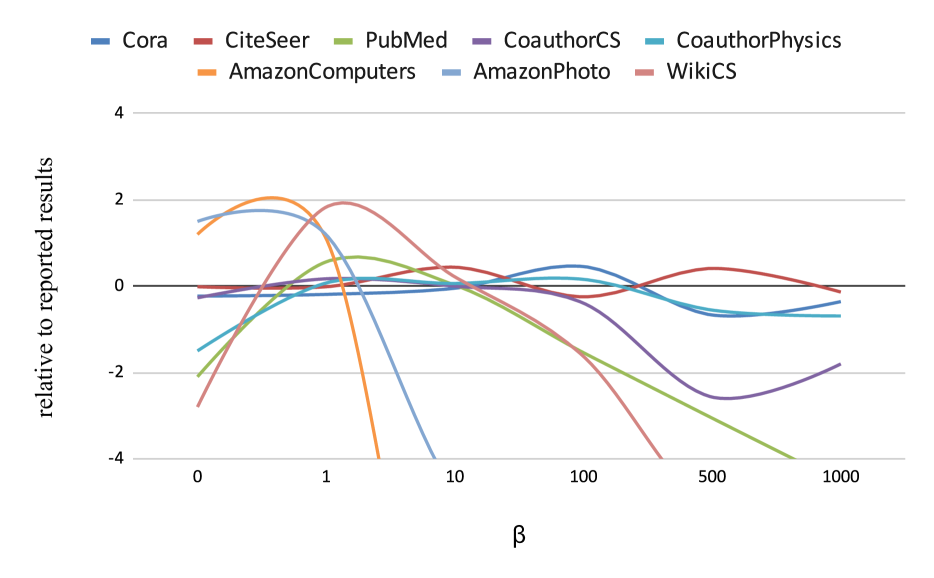
Figure 2: Effect of $\beta$ on transductive node classification performance. The vertical axis shows the performance in %, relative to the results reported in the main paper.

Figure 2 shows the effect of $\beta$ on transductive node classification for different datasets. For most of the datasets, the results are rather stable for quite a large range of $\beta$, i.e., in [1, 50] range. AmazonComputers and AmazonPhoto datasets are an exception in the sense that their performance degrades quicker than other datasets. Overall, a general trend of degradation can be observed for high values of $\beta$ for all datasets, which is intuitive because for such values, the covariance loss takes over and the reconstruction loss is practically neglected, resulting in relatively poor results. Another observation is that the results above the 0-line on the graphs are better than the ones reported in the main paper. So, by carefully tuning $\beta$, we can achieve even better results compared to the ones reported in the paper.

8.2 Effect of $\lambda$

The hyperparameter $\lambda$ governs the trade-off between invariance and cross-covariance in equation 9. The proposed value of $\lambda$ in [60] is $5e^{-3}$. To see the effect of changing $\beta$, we sweep it across the values $\{1e^{-3},5e^{-3},1e^{-2},5e^{-2}\}$. The effect of changing $\lambda$ on different datasets has been plotted in figure 3. The plot validates that $\lambda=5e^{-3}$, proposed in Barlow Twins[60], is a reasonable choice also for graph datasets. Some datasets perform better for $\lambda=1e^{-3}$ and some yield better results for $\lambda=1e^{-2}$. However, there is a general trend of decrease in the performance for $\lambda\geq 5e^{-2}$.

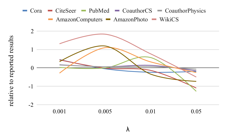
Figure 3: Effect of $\lambda$ on transductive node classification performance. The vertical axis shows the performance in %, relative to the results reported in the main paper.

8.3 Effect of Average Sparsification Degree in ${\mathbf{S}}$

As mentioned in section 2.3, one of the ways of sparsification is to provide the intended average node degree. We have fixed this value to 25 for all the reported results. Now we observe the effect of changing this hyperparameter. For this purpose, we sweep the average degree over the values $\{5,10,20,25,30,40,50,60,75,80,100,125,150\}$. The results have been plotted in figure 4. The results for PubMed are not plotted for the degree values greater than 75 because of out-of-memory issues. The relative performance remains more or less consistent over the plotted range, and varies between $\pm 1\%$ of the reported results. This also shows that the architecture can extract the relevant information from the neighborhood over a reasonable range of average degree. An exception is WikiCS where the results improve by up to 2% compared to the reported results in table 3 for the average degree value of 150. However, for such a high value, the graph is no longer reasonably sparse. This causes high training overhead because of the large number of edges in ${\mathbf{S}}$. On the other extreme, for the value of 5, we can see a decline in many datasets because here ${\mathbf{S}}$ is too sparse, hence the information in ${\mathbf{S}}$ is too little to be of use.

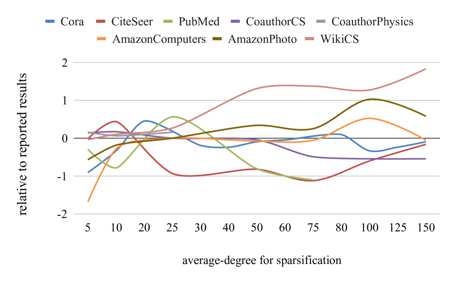
Figure 4: Effect of average node degree in ${\mathbf{S}}$ on transductive node classification performance. The vertical axis shows the performance in %, relative to the results reported in the main paper.

9 Variants of Our Approach

In the main paper, we have reported the results for PPR both with and without attention. From these results, we can already establish that it is always better to use attention i.e., let the neural network decide the weights for averaging the embeddings from the immediate and larger neighborhood. So, in this section, we focus on the case with attention, and report the results with following variations:

• Toggling $L_{\mathrm{recon}}$ on/off in equation 1

• Choosing between BGAE and BVGAE.

• Choosing between PPR and Heat Kernels for diffusion.

For brevity, we use triple of the form $\Big{(}\mathbf{1}(L_{\mathrm{recon}}\text{ is mute}),\mathbf{1}(\text{ variational model}),\text{kernel name}\Big{)}$. For instance, (1, 0, ppr) means that we are referring to the variant where we are only using $L_{\mathrm{cov}}$ in non-variational mode with PPR kernel for diffusion. In the main paper, we have reported the results for the variant (0, 0, ppr) and (0, 1, ppr). Using this notation, we plot the results for all the eight variations for all three tasks i.e. link prediction, clustering and transductive node classification in figure 5(a), figure 5(b), and figure 5(c) respectively. For some datasets (e.g., CoauthorPhysics), some variants could not be plotted because of out-of-memory issues. The general behavior is similar for different variants across all three tasks. The important observations from figure 5 are as follows:

• The variant (0, 0, ppr), shown in green, performs the best overall.

• The variants (0, 0, ppr) and (0, 0, heat) are usually close in performance, although (0, 0, ppr) is often better by a small margin.

• The variants (0, 0, ppr) and (0, 0, heat) with simple GCN encoders usually outperform their variational counterparts, i.e., (0, 1, ppr) and (0, 1, heat). There are, however, minor exceptions. For instance, in figure 5(a), (0, 1, ppr) is marginally better than (0, 0, ppr) for CiteSeer. Similarly, in figure 5(b), (0, 1, heat) is marginally better than (0, 0, heat) for CoauthorCS.

• When $L_{\mathrm{recon}}$ is turned off, the performance is usually relatively worse than when $L_{\mathrm{recon}}$ is on. This can be seen in (1, 1, ppr), (1, 0, ppr), (1, 1, heat), and (1, 0, heat) variants. The only exception is CiteSeer in figure 5(a) where (1, 1, ppr) outperforms (0, 1, ppr) by a tiny margin. This validates our intuition that $L_{\mathrm{recon}}$ aids $L_{\mathrm{cov}}$ almost always.

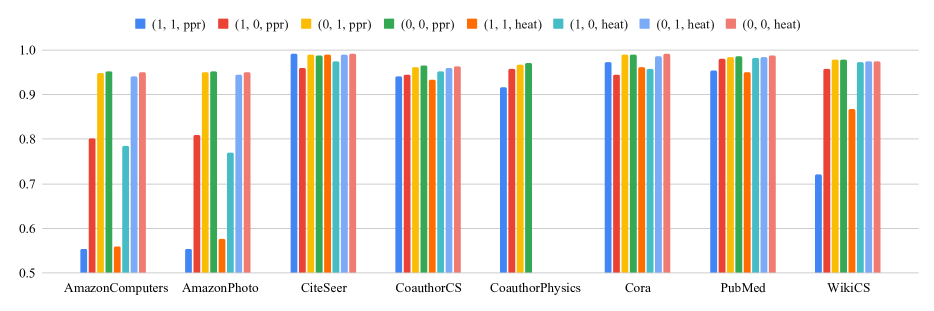
(a) Variants of our approach for link prediction

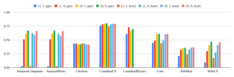
(b) Variants of our approach for node clustering

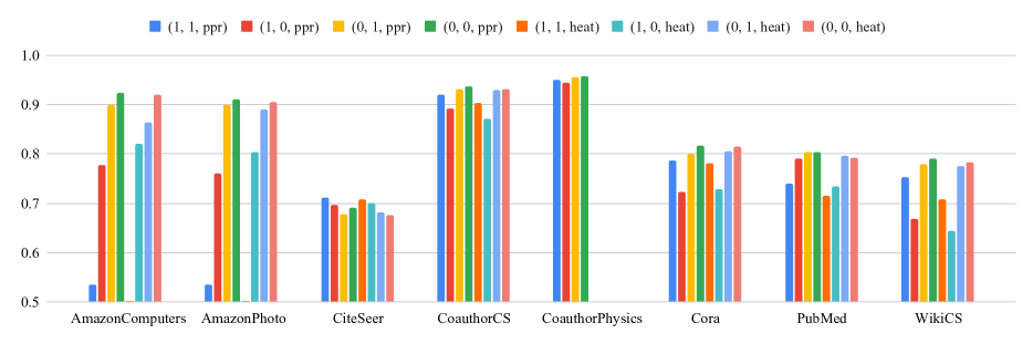
(c) Variants of our approach for node classification

Figure 5: Variants of our approach for link prediction, node clustering, and node classification.

References

- [1] Andersen, R., Chung, F., Lang, K.: Local graph partitioning using pagerank vectors. In: 2006 47th Annual IEEE Symposium on Foundations of Computer Science (FOCS’06). pp. 475–486. IEEE (2006)
- [2] Anonymous: Implementation code. https://github.com/AnoanonymizedForReview/bgae (Oct 2022)
- [3] Ata, S.K., Fang, Y., Wu, M., Li, X.L., Xiao, X.: Disease gene classification with metagraph representations. Methods 131, 83–92 (2017)
- [4] Barlow, H.B., et al.: Possible principles underlying the transformation of sensory messages. Sensory communication 1(01) (1961)
- [5] Bielak, P., Kajdanowicz, T., Chawla, N.V.: Graph barlow twins: A self-supervised representation learning framework for graphs. Knowledge-Based Systems p. 109631 (2022)
- [6] Cai, H., Zheng, V.W., Chang, K.C.C.: A comprehensive survey of graph embedding: Problems, techniques, and applications. IEEE Transactions on Knowledge and Data Engineering 30(9), 1616–1637 (2018)
- [7] Cao, S., Lu, W., Xu, Q.: Grarep: Learning graph representations with global structural information. In: Proceedings of the 24th ACM international on conference on information and knowledge management. pp. 891–900 (2015)
- [8] Cao, S., Lu, W., Xu, Q.: Deep neural networks for learning graph representations. In: Proceedings of the AAAI Conference on Artificial Intelligence. vol. 30 (2016)
- [9] Chami, I., Ying, Z., Ré, C., Leskovec, J.: Hyperbolic graph convolutional neural networks. Advances in neural information processing systems 32, 4868–4879 (2019)
- [10] Cui, P., Wang, X., Pei, J., Zhu, W.: A survey on network embedding. IEEE Transactions on Knowledge and Data Engineering 31(5), 833–852 (2018)
- [11] Defferrard, M., Bresson, X., Vandergheynst, P.: Convolutional neural networks on graphs with fast localized spectral filtering. Advances in neural information processing systems 29, 3844–3852 (2016)
- [12] Gilmer, J., Schoenholz, S.S., Riley, P.F., Vinyals, O., Dahl, G.E.: Neural message passing for quantum chemistry. In: International Conference on Machine Learning. pp. 1263–1272. PMLR (2017)
- [13] Grover, A., Leskovec, J.: node2vec: Scalable feature learning for networks. In: Proceedings of the 22nd ACM SIGKDD international conference on Knowledge discovery and data mining. pp. 855–864 (2016)
- [14] Grover, A., Zweig, A., Ermon, S.: Graphite: Iterative generative modeling of graphs. In: International conference on machine learning. pp. 2434–2444. PMLR (2019)
- [15] Gulcehre, C., Denil, M., Malinowski, M., Razavi, A., Pascanu, R., Hermann, K.M., Battaglia, P., Bapst, V., Raposo, D., Santoro, A., et al.: Hyperbolic attention networks. arXiv preprint arXiv:1805.09786 (2018)
- [16] Hamilton, W., Ying, Z., Leskovec, J.: Inductive representation learning on large graphs. In: Advances in neural information processing systems. pp. 1024–1034 (2017)
- [17] Hassani, K., Khasahmadi, A.H.: Contrastive multi-view representation learning on graphs. In: International Conference on Machine Learning. pp. 4116–4126. PMLR (2020)
- [18] Hjelm, R.D., Fedorov, A., Lavoie-Marchildon, S., Grewal, K., Bachman, P., Trischler, A., Bengio, Y.: Learning deep representations by mutual information estimation and maximization. arXiv preprint arXiv:1808.06670 (2018)
- [19] Jiang, B., Lin, D., Tang, J., Luo, B.: Data representation and learning with graph diffusion-embedding networks. In: Proceedings of the IEEE/CVF Conference on Computer Vision and Pattern Recognition. pp. 10414–10423 (2019)
- [20] Karrer, B., Newman, M.E.: Stochastic blockmodels and community structure in networks. Physical review E 83(1), 016107 (2011)
- [21] Khan, R.A., Anwaar, M.U., Kaddah, O., Han, Z., Kleinsteuber, M.: Unsupervised learning of joint embeddings for node representation and community detection. In: Machine Learning and Knowledge Discovery in Databases. Research Track. pp. 19–35. Springer International Publishing, Cham (2021)
- [22] Khan, R.A., Anwaar, M.U., Kleinsteuber, M.: Epitomic variational graph autoencoder (2020)
- [23] Kingma, D.P., Ba, J.: Adam: A method for stochastic optimization. arXiv preprint arXiv:1412.6980 (2014)
- [24] Kingma, D.P., Welling, M.: Auto-encoding variational bayes. arXiv preprint arXiv:1312.6114 (2013)
- [25] Kipf, T.N., Welling, M.: Semi-supervised classification with graph convolutional networks. arXiv preprint arXiv:1609.02907 (2016)
- [26] Kipf, T.N., Welling, M.: Variational graph auto-encoders. arXiv preprint arXiv:1611.07308 (2016)
- [27] Klicpera, J., Weißenberger, S., Günnemann, S.: Diffusion improves graph learning. Advances in Neural Information Processing Systems 32, 13354–13366 (2019)
- [28] Ma, K., Yang, H., Yang, H., Jin, T., Chen, P., Chen, Y., Kamhoua, B.F., Cheng, J.: Improving graph representation learning by contrastive regularization. arXiv preprint arXiv:2101.11525 (2021)
- [29] Mavromatis, C., Karypis, G.: Graph infoclust: Leveraging cluster-level node information for unsupervised graph representation learning. arXiv preprint arXiv:2009.06946 (2020)
- [30] McAuley, J., Targett, C., Shi, Q., Van Den Hengel, A.: Image-based recommendations on styles and substitutes. In: Proceedings of the 38th international ACM SIGIR conference on research and development in information retrieval. pp. 43–52 (2015)
- [31] Mehta, N., Duke, L.C., Rai, P.: Stochastic blockmodels meet graph neural networks. In: International Conference on Machine Learning. pp. 4466–4474. PMLR (2019)
- [32] Mernyei, P., Cangea, C.: Wiki-cs: A wikipedia-based benchmark for graph neural networks. arXiv preprint arXiv:2007.02901 (2020)
- [33] Oord, A.v.d., Li, Y., Vinyals, O.: Representation learning with contrastive predictive coding. arXiv preprint arXiv:1807.03748 (2018)
- [34] Ou, M., Cui, P., Pei, J., Zhang, Z., Zhu, W.: Asymmetric transitivity preserving graph embedding. In: Proceedings of the 22nd ACM SIGKDD international conference on Knowledge discovery and data mining. pp. 1105–1114 (2016)
- [35] Page, L., Brin, S., Motwani, R., Winograd, T.: The pagerank citation ranking: Bringing order to the web. Tech. rep., Stanford InfoLab (1999)
- [36] Pan, S., Hu, R., Long, G., Jiang, J., Yao, L., Zhang, C.: Adversarially regularized graph autoencoder for graph embedding. arXiv preprint arXiv:1802.04407 (2018)
- [37] Park, J., Lee, M., Chang, H.J., Lee, K., Choi, J.Y.: Symmetric graph convolutional autoencoder for unsupervised graph representation learning. In: Proceedings of the IEEE/CVF International Conference on Computer Vision. pp. 6519–6528 (2019)
- [38] Perozzi, B., Al-Rfou, R., Skiena, S.: Deepwalk: Online learning of social representations. In: Proceedings of the 20th ACM SIGKDD international conference on Knowledge discovery and data mining. pp. 701–710 (2014)
- [39] Qiu, J., Chen, Q., Dong, Y., Zhang, J., Yang, H., Ding, M., Wang, K., Tang, J.: Gcc: Graph contrastive coding for graph neural network pre-training. In: Proceedings of the 26th ACM SIGKDD International Conference on Knowledge Discovery & Data Mining. pp. 1150–1160 (2020)
- [40] Qu, M., Bengio, Y., Tang, J.: Gmnn: Graph markov neural networks. In: International conference on machine learning. pp. 5241–5250. PMLR (2019)
- [41] Ribeiro, L.F., Saverese, P.H., Figueiredo, D.R.: struc2vec: Learning node representations from structural identity. In: Proceedings of the 23rd ACM SIGKDD international conference on knowledge discovery and data mining. pp. 385–394 (2017)
- [42] Sen, P., Namata, G., Bilgic, M., Getoor, L., Galligher, B., Eliassi-Rad, T.: Collective classification in network data. AI magazine 29(3), 93–93 (2008)
- [43] Sinha, A., Shen, Z., Song, Y., Ma, H., Eide, D., Hsu, B.J., Wang, K.: An overview of microsoft academic service (mas) and applications. In: Proceedings of the 24th international conference on world wide web. pp. 243–246 (2015)
- [44] Tang, J., Qu, M., Wang, M., Zhang, M., Yan, J., Mei, Q.: Line: Large-scale information network embedding. In: Proceedings of the 24th international conference on world wide web. pp. 1067–1077 (2015)
- [45] Thakoor, S., Tallec, C., Azar, M.G., Azabou, M., Dyer, E.L., Munos, R., Veličković, P., Valko, M.: Large-scale representation learning on graphs via bootstrapping. arXiv preprint arXiv:2102.06514 (2021)
- [46] Tishby, N., Pereira, F.C., Bialek, W.: The information bottleneck method. arXiv preprint physics/0004057 (2000)
- [47] Veličković, P., Cucurull, G., Casanova, A., Romero, A., Lio, P., Bengio, Y.: Graph attention networks. arXiv preprint arXiv:1710.10903 (2017)
- [48] Velickovic, P., Fedus, W., Hamilton, W.L., Liò, P., Bengio, Y., Hjelm, R.D.: Deep graph infomax. aaa (2019)
- [49] Wang, C., Pan, S., Hu, R., Long, G., Jiang, J., Zhang, C.: Attributed graph clustering: A deep attentional embedding approach. arXiv preprint arXiv:1906.06532 (2019)
- [50] Wang, X., Cui, P., Wang, J., Pei, J., Zhu, W., Yang, S.: Community preserving network embedding. In: Thirty-first AAAI conference on artificial intelligence (2017)
- [51] Wei, Z., He, X., Xiao, X., Wang, S., Shang, S., Wen, J.R.: Topppr: top-k personalized pagerank queries with precision guarantees on large graphs. In: Proceedings of the 2018 International Conference on Management of Data. pp. 441–456 (2018)
- [52] Wu, Z.X., Xu, X.J., Chen, Y., Wang, Y.H.: Spatial prisoner’s dilemma game with volunteering in newman-watts small-world networks. Physical Review E 71(3), 037103 (2005)
- [53] Xia, R., Pan, Y., Du, L., Yin, J.: Robust multi-view spectral clustering via low-rank and sparse decomposition. In: Proceedings of the AAAI conference on artificial intelligence. vol. 28 (2014)
- [54] Xu, B., Shen, H., Cao, Q., Cen, K., Cheng, X.: Graph convolutional networks using heat kernel for semi-supervised learning. arXiv preprint arXiv:2007.16002 (2020)
- [55] Xu, K., Hu, W., Leskovec, J., Jegelka, S.: How powerful are graph neural networks? arXiv preprint arXiv:1810.00826 (2018)
- [56] Yang, C., Liu, Z., Zhao, D., Sun, M., Chang, E.: Network representation learning with rich text information. In: Twenty-fourth international joint conference on artificial intelligence (2015)
- [57] Yang, J., Leskovec, J.: Overlapping community detection at scale: a nonnegative matrix factorization approach. In: Proceedings of the sixth ACM international conference on Web search and data mining. pp. 587–596 (2013)
- [58] Yang, Z., Cohen, W., Salakhudinov, R.: Revisiting semi-supervised learning with graph embeddings. In: International conference on machine learning. pp. 40–48. PMLR (2016)
- [59] Ying, R., He, R., Chen, K., Eksombatchai, P., Hamilton, W.L., Leskovec, J.: Graph convolutional neural networks for web-scale recommender systems. In: Proceedings of the 24th ACM SIGKDD International Conference on Knowledge Discovery & Data Mining. pp. 974–983 (2018)
- [60] Zbontar, J., Jing, L., Misra, I., LeCun, Y., Deny, S.: Barlow twins: Self-supervised learning via redundancy reduction. arXiv preprint arXiv:2103.03230 (2021)
- [61] Zhang, X., Liu, H., Li, Q., Wu, X.M.: Attributed graph clustering via adaptive graph convolution. arXiv preprint arXiv:1906.01210 (2019)
- [62] Zheng, S., Zhu, Z., Zhang, X., Liu, Z., Cheng, J., Zhao, Y.: Distribution-induced bidirectional generative adversarial network for graph representation learning. In: Proceedings of the IEEE/CVF Conference on Computer Vision and Pattern Recognition. pp. 7224–7233 (2020)
- [63] Zhou, J., Cui, G., Hu, S., Zhang, Z., Yang, C., Liu, Z., Wang, L., Li, C., Sun, M.: Graph neural networks: A review of methods and applications. AI Open 1, 57–81 (2020)
- [64] Zhu, Y., Xu, Y., Yu, F., Liu, Q., Wu, S., Wang, L.: Deep graph contrastive representation learning. arXiv preprint arXiv:2006.04131 (2020)
- [65] Zhu, Y., Xu, Y., Yu, F., Liu, Q., Wu, S., Wang, L.: Graph contrastive learning with adaptive augmentation. In: Proceedings of the Web Conference 2021. pp. 2069–2080 (2021)