Droplet-superfluid compounds in binary bosonic mixtures

Abstract

While quantum fluctuations in binary mixtures of bosonic atoms with short-range interactions can lead to the formation of a self-bound droplet, for equal intra-component interactions but an unequal number of atoms in the two components, there is an excess part that cannot bind to the droplet. Imposing confinement, as here through periodic boundary conditions in a one-dimensional setting, the droplet becomes amalgamated with a residual condensate. The rotational properties of this compound system reveal simultaneous rigid-body and superfluid behavior in the ground state and uncover that the residual condensate can carry angular momentum even in the absence of vorticity. In contradiction to the intuitive idea that the superfluid fraction of the system would be entirely made up of the excess atoms not bound by the droplet, we find evidence that this fraction is higher than what one would expect in such a picture. Our findings are corroborated by an analysis of the elementary excitations in the system, and shed new light on the coexistence of localization and superfluidity.

In the field of ultra-cold atomic quantum gases it was suggested early-on Bulgac (2002); Bedaque et al. (2003); Hammer and Son (2004) that quantum effects beyond mean-field (BMF) may lead to self-bound droplets of fermionic or bosonic atoms. For weakly-interacting single-component Bose gases, quantum fluctuations alone are often too small to play any significant role. Nevertheless, for binary or dipolar Bose gases the interactions may be adjusted such that the different main contributions to the mean-field (MF) energy nearly cancel out, leaving only a small residual term that can be tuned to equilibrate with the BMF part of the total energy. A self-bound dilute boson droplet may then form Petrov (2015); Petrov and Astrakharchik (2016), with curious properties originating from its genuine quantum many-body nature. Although originally proposed for binary Bose gases Petrov and Astrakharchik (2016), the first experimental observations of droplets stabilized by the Lee-Huang-Yang (LHY) quantum fluctuations Lee et al. (1957) were made for strongly dipolar atoms such as Dysprosium Kadau et al. (2016); Ferrier-Barbut et al. (2016a, b); Schmitt et al. (2016) and Erbium Chomaz et al. (2016). Here, a scenario similar to the binary case Staudinger et al. (2018) arises due to the peculiarities of the dipolar interactions Wächtler and Santos (2016a, b); Macia et al. (2016); Bisset et al. (2016); Baillie et al. (2017). Experiments with binary bosonic mixtures of potassium Cabrera et al. (2018); Semeghini et al. (2018); Cheiney et al. (2018) or hetero-nuclear mixtures D’Errico et al. (2019); Guo et al. (2021) followed soon after (for brief reviews on droplet formation, see Refs. Böttcher et al. (2021); Luo et al. (2021)). In low-dimensional systems, quantum fluctuations may be enhanced, facilitating and stabilizing the droplet formation process Petrov and Astrakharchik (2016); Astrakharchik and Malomed (2018); Parisi et al. (2019), and the dimensional crossover has been discussed in Refs. Zin et al. (2018); Ilg et al. (2018); Lavoine and Bourdel (2021). Recent work on binary self-bound states in 1D or quasi-1D also investigated corrections beyond LHY Ota and Astrakharchik (2020), applied the quantum Monte-Carlo method Parisi et al. (2019); Parisi and Giorgini (2020), used the Bose Hubbard model Morera et al. (2020, 2021a) or formulated an effective quantum field theory Chiquillo (2018). It has been shown that microscopic pairing or dimer models agree with variational approaches Hu et al. (2020); Morera et al. (2021b). Collective excitations Cappellaro et al. (2018); Tylutki et al. (2020) and thermodynamic properties Ota and Astrakharchik (2020); De Rosi et al. (2021) were also studied.
Droplets may also form in systems with inter-component asymmetry. One obvious realization is heteronuclear mixtures, see e.g. Refs. Ancilotto et al. (2018); D’Errico et al. (2019); Minardi et al. (2019); Guo et al. (2021); Mistakidis et al. (2021). Another interesting scenario arises when the intra-component interactions are equal, but the components have different numbers of particles. Then, the excess particles in the larger component cannot bind to the droplet Petrov (2015), but instead form a uniform background into which the droplet is immersed Mithun et al. (2020). In a similar line of thought, but for non-equal interactions within the components, it was recently suggested Naidon and Petrov (2021) that a mixed phase may coexist with a non-amalgamated gaseous component, where partial miscibility is caused by BMF contributions leading to so-called “bubble” phases with similarities to the droplet self-bound states.

In this Letter, we set focus on the case of asymmetric components confined in a one-dimensional trap with periodic boundary conditions. For equal intra-species interactions but different numbers of particles in the two components, with increasing coupling strength the translational symmetry of the uniform system is broken. A localized droplet forms, stabilized by quantum fluctuations, which coexists with a uniform residual condensate of excess atoms that cannot bind to the droplet, but are kept together by the confinement. We demonstrate that this asymmetric system, although with just a single droplet unlike what is typically seen in dipolar supersolids Böttcher et al. (2021), simultaneously exhibits rigid-body and superfluid properties. The non-classical rotational inertia (NCRI) reveals that the motion of the droplet at low velocities is not only that of a classical rigid body but is accompanied by the response of the non-droplet atoms moving in a direction opposite to the motion of the rigid body. Importantly, this response is found to exist for infinitesimal rotations, thus having a profound impact on the degree of superfluidity of the system. The number of atoms contributing to the formation of a vortex is larger than that of the residual condensate, coinciding with the NCRI fraction. Our findings are corroborated by an analysis of the lowest excitation modes in the compound system.
The energy density for a uniform binary Bose-Bose mixture in one dimension with equal masses and short-ranged interactions, including BMF corrections, equals Petrov and Astrakharchik (2016)

$$\mathcal{E}=\frac{g}{2}(n_{1}^{2}+n_{2}^{2})+(\delta g-g)n_{1}n_{2}-\frac{2m^{1/2}g^{3/2}}{3\pi\hbar}(n_{1}+n_{2})^{3/2},$$ (1)

where $n_{i}$ are the densities of each component and $m$ the mass of a single particle. Here we have set the intraspecies coupling constants to be equal, $g_{11}=g_{22}=g$, and introduced $\delta g=g+g_{12}$, where $g_{12}$ is the interspecies coupling constant. The first two terms in Eq. (1) constitute the MF energy density and the last term accounts for the first correction beyond mean field. The energy density Eq. (1) is valid provided $\eta=\sqrt{mg/n\hbar^{2}}\ll 1$, ensuring weak interactions (here we have assumed similar order of magnitudes for the densities $n_{1}\sim n_{2}\sim n$), and that $\delta g$ is small in the sense $\delta g/g\sim\eta$. For a finite-size system the extended coupled Gross-Pitaevskii equations corresponding to the energy density Eq. (1) are

$$\mathrm{i}\hbar\partial_{t}\psi_{i}= -\frac{\hbar^{2}}{2m}\partial_{xx}\psi_{i}+g|\psi_{i}|^{2}\psi_{i}+(\delta g-g)|\psi_{j}|^{2}\psi_{i}$$ (2)

$$-\frac{m^{1/2}g^{3/2}}{\pi\hbar}(|\psi_{i}|^{2}+|\psi_{j}|^{2})^{1/2}\psi_{i}~{},$$

where $i,j=1,2$ and $i\neq j$. We impose periodic boundary conditions $\psi_{i}(x)=\psi_{i}(x+2\pi R)$, enforcing a confinement of length $2\pi R$. This is a good approximation for a ring of radius $R$ whenever bending effects may be neglected, i.e. when the transversal confinement length is much smaller than $R$. (Such binary 1D ring systems have been extensively studied, both experimentally Ryu et al. (2007); Ramanathan et al. (2011); Wright et al. (2013); Ryu et al. (2013); Beattie et al. (2013); Eckel et al. (2014); Guo and Pfau (2020); Nicolau et al. (2020) and theoretically  Smyrnakis et al. (2009, 2012); Anoshkin et al. (2013); Smyrnakis et al. (2014); Abad et al. (2014); Muñoz Mateo et al. (2015); Roussou et al. (2018); Chen et al. (2019); Polo et al. (2019); Ögren et al. (2021)).
From here on, we use dimensionless units such that $\hbar=m=R=1$. The order parameter is normalized to the number of particles in each component according to $\int_{0}^{2\pi}|\psi_{i}(x)|^{2}\mathrm{d}x=N_{i}$. The ground state is obtained by solving Eq. (2) numerically with a split-step Fourier method in imaginary time. To analyze the system in a rotating frame the term $-\Omega\hat{L}\psi_{i}$ is added to the right side of Eq. (2), where $\hat{L}=-\mathrm{i}\partial_{x}$, which is then solved in the same manner. In order to find the ground state for a fixed value of the angular momentum $L=L_{1}+L_{2}$, where $L_{i}=\int_{0}^{2\pi}\psi^{\ast}_{i}\hat{L}\psi_{i}\mathrm{d}x$, we consider the quantity $\tilde{E}=E+(C/2)(L-L_{0})^{2}$ Komineas et al. (2005), where $E$ is the total energy corresponding to Eq. (2). By minimizing $\tilde{E}$ for sufficiently large values of the constant $C>0$, the obtained ground state will have angular momentum $L\approx L_{0}$ since the critical point of $\tilde{E}$ is $L=L_{0}-\partial_{L}E/C$, which is a minimum whenever $C>-\partial_{LL}E$. Introducing $\lambda=\delta g/g$, $N=N_{1}+N_{2}$ and $\nu=N_{2}/N_{1}$, we illustrate our findings below by fixing $\lambda=0.01$ and $N=5000$. The asymmetry parameter is restricted to $\nu\geq 1$.
We first investigate the density distributions of the two components, starting with the symmetric case where both components of the mixture are equal, $\nu=1$. The upper panel of Fig. 1 shows the corresponding densities for different values of the interaction parameter $g$ for a slowly rotating system. For high enough values of $g$ the ground state has the form of a droplet in agreement with previous findings in one dimension Petrov and Astrakharchik (2016); Astrakharchik and Malomed (2018). As $g$ is decreased the extent of the droplet increases, which results in a transition to a uniform state. We understand this by considering the bulk density of a flat-top droplet $n_{0}=8g/(9\pi^{2}\lambda^{2})$ Petrov and Astrakharchik (2016), which implies a droplet extent $\sim N/(2n_{0})$. When this droplet size is much smaller than the ring length the periodic boundary conditions do not significantly affect the system. As $g$ is decreased, the droplet size eventually becomes comparable to the ring length for $g\sim 9\pi N\lambda^{2}/32$. This results in a transition from a droplet to a uniform system and is a consequence of the periodic boundary conditions. (See also the discussion of boundary effects in Cui and Ma (2021)). For low values of $g$, the situation is similar also in the asymmetric case, where both components display uniform behavior, as shown for $\nu=3$ in the lower panel of Fig. 1. With increasing interaction strength $g$ the translation symmetry is eventually broken, and the ground state density for the component with more particles changes to what appears to be a mix between a droplet and a uniform medium, while the other component displays a normal droplet solution. The droplet coexists with a uniform background, since the excess particles in the second component can not bind to it Petrov (2015). Deviating from $\nu=1$ results in an increase in the ratio of MF to BMF energy, eventually causing the former to dominate the total energy. Thus, unlike the symmetric case where droplet formation takes place where the MF and BMF terms are of similar orders of magnitude, for the asymmetric system we have BMF effects such as displayed in Fig. 1 even though the MF contribution can be much larger than the BMF one. We note that solving Eq. (2) without the BMF contribution ceteris paribus leads to uniform solutions in the regimes where non-uniform ones were obtained with the full Eq. (2) for our choice of parameters.

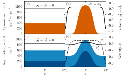
Figure 1: (Color online) Condensate densities $|\Psi_{i}|^{2}$ (red, blue) and velocities $\phi_{i}^{\prime}$ (black lines) of the two components in the rotating frame where $\Omega=0.1$. The upper panel shows the symmetric case, $\nu=1$. (a) $|\Psi_{1}|^{2}=|\Psi_{2}|^{2}$ for $g=0.5$ (red), being homogeneous along the ring. (b) as in (a) but for $g=1.2$, showing droplet formation. The lower panel shows the asymmetric case for $\nu=3$ for the same parameters as in the upper panel. The axis to the right in both panels shows the corresponding condensate velocities $\phi_{i}^{\prime}$.

We are here interested in the properties of this mixed-phase system. The ground-state energy $E(\ell)$ as a function of the angular momentum per particle $\ell$ is shown in Fig. 2 for different degrees of asymmetry $\nu$. It takes the form of a single parabola for $\nu=1$, corresponding to the rigid-body rotation of the droplet in the ring. For the asymmetric case with $\nu>1$, different parabolae appear to intersect. Intriguingly, the structure of $E(\ell)$ is similar to the one found for a dipolar toroidal system in three dimensions in the supersolid phase Nilsson Tengstrand et al. (2021). With this analogy in mind, we model the system by considering $N_{c}$ particles taking angular momentum as a classical rigid body under rotation and $N_{v}$ particles taking angular momentum only in terms of vorticity, with $N=N_{c}+N_{v}$.

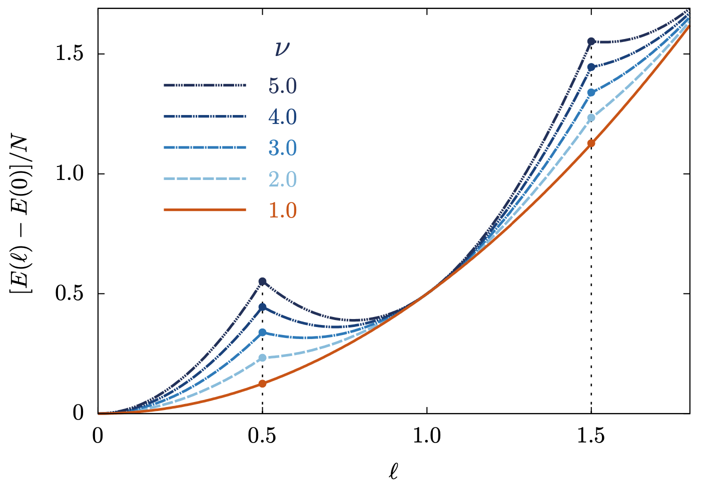
Figure 2: (Color online) Energy as a function of angular momentum per particle for $\nu=1,2,3,4,5$ as indicated by the legend, where $g=1.5$.

The energy cost for adding a vortex with $s$-fold quantization to the condensate can be determined by assuming an order parameter for the vortex component on the form $\propto\hbox{e}^{\mathrm{i}sx}$, where the integer $s$ is the angular momentum per particle in the vortex-carrying component, leading to an energy cost equal to $N_{v}s^{2}/2$. Since the solid-like part of the system carries angular momentum according to $N_{c}\ell_{c}^{2}/2$, where $\ell_{c}$ is its angular momentum per particle and $N\ell=N_{c}\ell_{c}+N_{v}s$, the different energetic branches dependent on angular momentum can be written

$$E_{s}/N=\frac{1}{2}\left[\frac{(\ell-f_{v}s)^{2}}{1-f_{v}}+f_{v}s^{2}\right],$$ (3)

where we have defined the fraction of particles carrying vorticity $f_{v}=N_{v}/N$. The branches $E_{s}$ and $E_{s+1}$ intersect at $\ell=s+1/2$, i.e., having no vortex is energetically favorable for $\ell~{}<~{}0.5$, having a singly-quantized one for $0.5<\ell<1.5$ and so on. The energies in Eq. (3) obtained within our model predict that the functional form of the dispersion relation should be parabolae intersecting at half-integer values of $\ell$, in accordance with the numerical results displayed in Fig. 2. Importantly, this suggests that the asymmetric system can exhibit properties of a solid and superfluid simultaneously, with rigid-body rotation and quantized vorticity coexisting. Unlike ring-shaped dipolar supersolids, which display a similar behavior under rotation Roccuzzo and Ancilotto (2019); Nilsson Tengstrand et al. (2021), here in the case of isotropic short-range interactions the ground state density does not exhibit any repeating crystalline structure. Since the branches $E_{s}$ have minima at $\ell=f_{v}s$, there is a possibility for the system to exhibit metastable superflow. These minima exist in the ground state energy $E(\ell)$ only if they occur on the interval where the corresponding branch $E_{s}(\ell)$ is the lowest in energy, thus giving a criterion for the existence of a metastable persistent current related to an $s$ times multiply-quantized vortex according to $f_{v}>(2s-1)/(2s)$.
It is tempting to identify the amount of particles belonging to the vortex component with the number $N_{2}-N_{1}$, intuitively imagining that $N_{1}$ particles from each component bind as a droplet and thus act in a solid-body fashion while the excess particles take the role of a background superfluid capable of carrying vorticity. If this were true, then $f_{v}=(N_{2}-N_{1})/N=(\nu-1)/(\nu+1)$, in contradiction with the numerically obtained positions of the minima in Fig. 2 which were predicted to occur at $\ell=f_{v}s$. To give an example, for $\nu=3$ the first minimum occurs at $\ell\approx 0.63$ while $(\nu-1)/(\nu+1)=0.5$. To investigate this obvious discrepancy, we compute the non-classical rotational inertia fraction for each component Leggett (1998)

$$f_{i}=1-\lim_{\Omega\to 0}\frac{L_{i}}{N_{i}\Omega}~{}.$$ (4)

The total NCRI fraction is defined as $f=(N_{1}f_{1}+N_{2}f_{2})/N$, and we plot the numerically obtained results in Fig. 3 for $\nu=1$ and $\nu=3$. Interestingly, for $\nu=1$ there is a discontinuous jump from $f=1$ to a value that is non-zero, signaling that even for the symmetric droplet system there are parameter values such that the motion is not entirely classical. As $\nu$ is increased the discontinuity decreases until it eventually disappears, as exemplified for $\nu=3$ in Fig. 3. We see that the total NCRI fraction for the asymmetric system not only differs from $(\nu-1)/(\nu+1)$ but is also dependent on $g$.

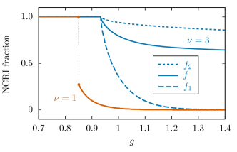
Figure 3: (Color online) Non-classical rotational inertia (NCRI) fraction as a function of interaction strength $g$ for $\nu=1$ (orange; the discontinuity is indicated by the bullets and connecting dashed line), and for $\nu=3$ with $f_{1},f_{2}$ and $f$ as indicated in the legend. (Note that $f=f_{1}=f_{2}$ for the symmetric system).

Let us now study the motion of the condensate under rotation by examining the condensate velocity $\phi_{i}^{\prime}(x)$ (where $\phi_{i}$ is the phase of the order parameter) which can be written

$$\phi_{i}^{\prime}(x)=\Omega+\frac{L_{i}-N_{i}\Omega}{2\pi n_{i}(x)}~{},$$ (5)

see Appendix A. The velocities for some parameters are plotted in Fig. 1 where in particular panels (b) and (d) show how the velocity for both components in the symmetric system and the first component in the asymmetric one are equal to $\Omega$ throughout most of the ring, reflecting the solid-like movement. Away from the bulk of the droplet where the density is small, the second term in Eq. (5) becomes significant and the velocity thus deviates from $\Omega$ in a manner depending on $L_{i}-N_{i}\Omega$. For small $\Omega$ this difference is negative, resulting in a change of sign for the velocity as displayed in Fig. 1(b) and (d). If the density is negligible in the region where the velocity deviates from $\Omega$ this will have little effect, but if the droplet instead occupies most of the ring, as is the case close to the transition point between the uniform and droplet phases, this results in parts of the system moving in a direction opposite to the rest of the condensate. The NCRI fraction will consequently differ from zero, explaining why $f$ for the symmetric system and $f_{1}$ for the asymmetric system do not immediately fall to zero at the transition point. For the second component in the non-uniform asymmetric case the velocity has opposite signs inside and outside the droplet region, indicating that the movement of the droplet is accompanied by a response of the background medium, which moves in the other direction. Since this response exists also for infinitesimal rotations, it affects the results based on the definition in Eq. (4), increasing it compared to if there had been no response flow of the background. Curiously, this implies that the interpretation of $f$ as the fraction of particles that stay at rest as the container is set to slowly rotate is not a correct one. (Interestingly, a similar type of response by the background has been noticed also for dipolar condensates in the supersolid phase Roccuzzo et al. (2020); Nilsson Tengstrand et al. (2021)). To connect to the results in Fig. 2, we compute the corresponding NCRI fractions and find that $f\approx 0.47$, $f\approx 0.63$, $f\approx 0.72$ and $f\approx 0.78$ for $\nu=2,3,4,5$, respectively. These data agree well with the positions of the minima of $E(\ell)$, suggesting that $f_{v}\approx f$, i.e., that the fraction of particles related to vortex formation is larger than that of the residual condensate and coincides with the NCRI fraction. Finally, we investigate the spectra of collective excitations. Following the usual procedure we linearize the extended Gross-Pitaevskii equation Eq. (2) around the ground state $\psi_{0,i}$ and write

$$\psi_{i}(x,t)=\mathrm{e}^{-\mathrm{i}\mu_{i}t}\left[\psi_{0,i}(x)+u_{i}(x)\mathrm{e}^{-\mathrm{i}\omega t}+v_{i}^{\ast}(x)\mathrm{e}^{\mathrm{i}\omega t}\right]~{},$$ (6)

keeping terms up to first order in the Bogoliubov amplitudes $u_{i}$ and $v_{i}$. Here $\mu_{i}$ is the chemical potential and $\omega/(2\pi)$ is the frequency of oscillation of $u_{i}$ and $v_{i}$. Due to the periodic boundary conditions imposed on the system, we expand the amplitudes in plane waves according to $u_{i}(x)=\mathrm{e}^{\mathrm{i}kx}u_{i,k}(x)$ and $v_{i}(x)=\mathrm{e}^{\mathrm{i}kx}v_{i,k}(x)$ allowing us to solve the resulting Bogoliubov-de Gennes equations for fixed $k$ (see Appendix B for more details). Fig. 4 shows the lowest modes as a function of $k$ for the symmetric ($\nu=1$) and asymmetric case (here for $\nu=4$) in the non-uniform regime. In both cases there are three gapless modes, which we characterize by looking at the density and phase fluctuations of the system, $\Delta n_{i,k}=|u_{i,k}+v_{i,k}|^{2}$ and $\Delta\phi_{i,k}=|u_{i,k}-v_{i,k}|^{2}$, respectively Wu and Griffin (1996); Roccuzzo and Ancilotto (2019). Two of these modes are imaginary, indicating a dynamical instability of the system. As $g$ is decreased and we approach the uniform regime these modes harden, implying a higher degree of instability closer to the phase boundary. With increased $g$ the modes instead soften until they become vanishingly small and the system thus becomes stable. The softer of the imaginary modes is at $k=0$ a phase mode, and remains so for $\nu=1$ at all $k$. For $\nu=4$, the characteristics of this mode changes as $k$ is increased, and the component with more particles is instead dominated by fluctuations in the density while the component with fewer particles still is related to fluctuations in the phase. The harder of the imaginary modes is in all cases a density mode, corresponding to a center of mass excitation of the droplet.

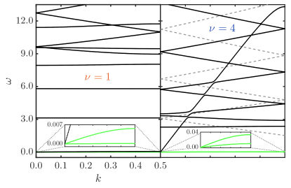
Figure 4: (Color online) Spectra of elementary excitations for $\nu=1$ (left panel) and $\nu=4$ (right panel) as a function of $k$ for $g=1.4$. The inset shows a zoom-in of the two lowest (green) modes (which are purely imaginary). The (gray) dashed lines show the analytical solutions in the homogeneous regime for $|p|\geq 3$ as discussed in the text for the corresponding parameter values.

The single real gapless mode is a phase mode that is related to the superfluidity of the system. For the symmetric case, it becomes soft rapidly as the NCRI goes to zero. With increasing $\nu$ the superfluid character of the condensate is enhanced, hardening this mode such that it may no longer be the lowest-lying one, resulting in both crossings and avoided crossings with the gapped modes, see the right panel of Fig. 4. The lowest-lying gapped modes of the pure droplet system are characterized by their insensitivity to $k$, the first one being the breathing mode Tylutki et al. (2020). For the asymmetric system we find that the lowest gapped mode is still the breathing mode, followed by higher modes with linear slopes that form a zig-zag pattern higher up in the spectrum. We can understand this structure from the solution of the Bogoliubov-de Gennes equations of the uniform condensate, which may be obtained analytically (see Appendix B). In this case the low-lying part of the spectrum is dominated by solutions on the form $\omega_{pk}\approx p^{2}/2+G+pk$, where $p$ is an integer and $G$ a number that depends only on the interaction strengths and particle numbers but not on $p$ or $k$. Figure 4 clearly shows how the non-uniform system exhibits a structure that is similar to the uniform one, but displaced to higher energies. This is a clear indication for the increased importance of the non-droplet superfluid background higher up in the excitation spectrum.
In conclusion, we have studied the effects of quantum fluctuations beyond just droplet formation of a one-dimensional binary Bose mixture with short-range interactions in a 1D confinement with periodic boundary conditions. Although the BMF contribution for asymmetric configurations may be small compared to the MF one, it can cause a transition to a system where translational symmetry is broken. Examining the rotational properties and collective excitations we found that droplet and superfluid characteristics co-exist. Through energetic considerations and from calculating the non-classical rotational inertia we demonstrated that the non-droplet part may not be simply identified as the total superfluid, due to its reaction to the droplet’s movement. Investigating the collective excitations revealed the existence of a single real gapless phase mode that softens with decreased NCRI, tying it to the degree of superfluidity of the system. Further superfluid signatures were observed in the spectrum of the non-uniform asymmetric system at higher energies where the structure became qualitatively similar to that of a homogeneous one. Although the present study focused on 1D, the results are expected to hold also in the quasi-1D limit for a sufficiently strong transversal trapping. As mentioned above, droplets have been experimentally observed for binary ³⁹K Cabrera et al. (2018); Semeghini et al. (2018), or hetero-nuclear mixtures D’Errico et al. (2019); Guo et al. (2021), and have also been confined in a quasi-1D optical waveguide Cheiney et al. (2018). A ring-shaped superfluid similar to what was envisioned here should thus be straight-forward to realize experimentally. Annular flow with long lifetime was realized in anharmonic traps Guo et al. (2020), and ring traps with widely tunable parameters were recently reported in Ref. de Goër de Herve et al. (2021), although for a single-component BEC. In the light of these recent experiments, the realization of toroidal droplet-superfluid compounds is a realistic endeavor, opening up for new insight regarding the coexistence of solid-like and superfluid properties.

Acknowledgments. This research was financially supported by the Knut and Alice Wallenberg Foundation, and the Swedish Research Council.

Appendix A Condensate Velocity

The time-independent coupled extended Gross-Pitaevskii equations in the rotating frame are

$$\mu_{i}\psi_{i}= -\frac{1}{2}\psi^{\prime\prime}_{i}+g|\psi_{i}|^{2}\psi_{i}+(\delta g-g)|\psi_{j}|^{2}\psi_{i}$$ (7)

$$-\frac{g^{3/2}}{\pi}(|\psi_{i}|^{2}+|\psi_{j}|^{2})^{1/2}\psi_{i}-\Omega\hat{L}\psi_{i},$$

where $\mu_{i}$ is the chemical potential and it is assumed that $i\neq j$ as in the main text. Writing $\psi_{i}(x)=\tilde{\psi}_{i}(x)\mathrm{e}^{\mathrm{i}\phi_{i}(x)}$ and inserting into Eq. (7) we find

$$\mu_{i}\tilde{\psi}_{i}= -\frac{1}{2}\tilde{\psi}_{i}^{\prime\prime}+\frac{1}{2}\tilde{\psi}_{i}(\phi_{i}^{\prime})^{2}+g\tilde{\psi}_{i}^{3}+(\delta g-g)\tilde{\psi}_{j}^{2}\tilde{\psi}_{i}$$ (8)

$$-\frac{g^{3/2}}{\pi}(\tilde{\psi}_{i}^{2}+\tilde{\psi}_{j}^{2})^{1/2}\psi_{i}-\Omega\tilde{\psi}_{i}\phi_{i}^{\prime}$$

$$+\mathrm{i}\left(-\tilde{\psi}_{i}^{\prime}\phi_{i}^{\prime}-\frac{1}{2}\tilde{\psi}_{i}\phi_{i}^{\prime\prime}+\Omega\tilde{\psi}_{i}^{\prime}\right).$$

Using the fact that $\tilde{\psi}_{i}$ and $\phi_{i}$ are real we separate Eq. (8) into two equations by identifying real and imaginary terms, where the imaginary part yields the equation

$$\frac{1}{2}\tilde{\psi}_{i}\phi_{i}^{\prime\prime}+\tilde{\psi}_{i}^{\prime}\phi_{i}^{\prime}=\Omega\tilde{\psi}_{i}^{\prime}.$$ (9)

This equation can be solved for $\phi_{i}^{\prime}(x)$ in terms of $\tilde{\psi}_{i}(x)$, with the solution

$$\phi_{i}^{\prime}(x)=\Omega+\frac{C_{i}}{n_{i}(x)},$$ (10)

where $C_{i}$ is an integration constant and $n_{i}=~{}|\psi_{i}|^{2}=~{}\tilde{\psi}_{i}^{2}$. Since the angular momentum can be written $L_{i}=\int n_{i}(x)\phi_{i}^{\prime}(x)\mathrm{d}x$ we finally obtain

$$\phi_{i}^{\prime}(x)=\Omega+\frac{L_{i}-N_{i}\Omega}{2\pi n_{i}(x)},$$ (11)

which is the expression for the condensate velocity used in the main text.

Appendix B Bogoliubov-de Gennes Equations

The extended Gross-Pitaevskii equation Eq. (4) of the main text is linearized around the ground state $\psi_{0,i}$ by writing

$$\psi_{i}(x,t)=\mathrm{e}^{-\mathrm{i}\mu_{i}t}\left[\psi_{0,i}(x)+u_{i}(x)\mathrm{e}^{-\mathrm{i}\omega t}+v_{i}^{\ast}(x)\mathrm{e}^{\mathrm{i}\omega t}\right]$$ (12)

and keeping terms up to first order in the Bogoliubov amplitudes $u_{i}$ and $v_{i}$ (here $\omega/2\pi$ is the frequency of oscillation of $u$ and $v$). Due to the periodicity of the system we expand the amplitudes in plane waves $u_{i}(x)=\mathrm{e}^{\mathrm{i}kx}u_{i,k}(x)$ and $v_{i}(x)=\mathrm{e}^{\mathrm{i}kx}v_{i,k}(x)$, resulting in the Bogoliubov-de Gennes equations

$$\mathbf{A}_{k}\mathbf{v}_{k}=\omega_{k}\mathbf{v}_{k},$$ (13)

where $\mathbf{v}_{k}=\begin{pmatrix}u_{1,k}(x)&v_{1,k}(x)&u_{2,k}(x)&v_{2,k}(x)\end{pmatrix}^{\mathrm{T}}$ and

$$\mathbf{A}_{k}=\begin{pmatrix}X_{12,k}&Y_{1}&Z&Z\\ -Y_{1}&-X_{12,k}&-Z&-Z\\ Z&Z&X_{21,k}&Y_{2}\\ -Z&-Z&-Y_{2}&-X_{21,k}\end{pmatrix}$$ (14)

with

$$X_{ij,k} =-\frac{1}{2}\frac{\partial^{2}}{\partial x^{2}}-\mathrm{i}k\frac{\partial}{\partial x}+\frac{k^{2}}{2}-\mu_{i}$$ (15)

$$+(2g-3\alpha)\psi_{0,i}^{2}+(\delta g-g-2\alpha)\psi_{0,j}^{2}$$

$$Y_{i} =(g-\alpha)\psi_{0,i}^{2}$$

$$Z =(\delta g-g-\alpha)\psi_{0,1}\psi_{0,2}$$

and

$$\alpha=\frac{g^{3/2}}{2\pi(\psi_{0,1}^{2}+\psi_{0,2}^{2})^{1/2}}.$$ (16)

Here $\alpha$ is the contribution due to beyond mean-field effects and we have assumed $\psi_{0,i}$ to be real. In the homogeneous regime the BdG equations can be solved analytically by writing Gao and Cai (2019)

$$\mathbf{v}_{k}(x)=\sum_{p=-\infty}^{\infty}\frac{e^{\mathrm{i}px}}{\sqrt{2\pi}}\tilde{\mathbf{v}}_{pk},$$ (17)

where $\mathbf{\tilde{v}}_{pk}=\begin{pmatrix}\tilde{u}_{1,pk}&\tilde{v}_{1,pk}&\tilde{u}_{2,pk}&\tilde{v}_{2,pk}\end{pmatrix}^{\mathrm{T}}$. By substituting into Eq. (13) it can be seen that $\mathrm{e}^{\mathrm{i}px}\tilde{\mathbf{v}}_{pk}/\sqrt{2\pi}$ is an eigenvector with eigenvalue $\omega_{pk}$ satisfying

$$\tilde{\mathbf{A}}_{pk}\tilde{\mathbf{v}}_{pk}=\omega_{pk}\tilde{\mathbf{v}}_{pk},$$ (18)

where

$$\tilde{\mathbf{A}}_{pk}=\begin{pmatrix}\tilde{X}_{1,pk}&Y_{1}&Z&Z\\ -Y_{1}&-\tilde{X}_{1,pk}&-Z&-Z\\ Z&Z&\tilde{X}_{2,pk}&Y_{2}\\ -Z&-Z&-Y_{2}&-\tilde{X}_{2,pk}\end{pmatrix},$$ (19)

and $\tilde{X}_{i,pk}=(p+k)^{2}/2+(g-\alpha)n_{i}$ with $n_{i}=N_{i}/(2\pi)$. The solutions to Eq. (18) are

$$\omega_{\pm,pk}^{2}=\frac{(p+k)^{2}}{4\pi}\bigg{[}\pi(p+k)^{2}+(g-\alpha)N$$ (20)

$$\pm\sqrt{(g-\alpha)^{2}(N_{1}-N_{2})^{2}+4(\delta g-g-\alpha)^{2}N_{1}N_{2}}\bigg{]},$$

which in the limit $g\gg\delta g,\alpha$ can be written

$$\omega_{+,pk}^{2}\approx\frac{(p+k)^{2}}{4\pi}\bigg{[}\pi(p+k)^{2}+2(g-\alpha)N-4(\delta g-2\alpha)\frac{N_{1}N_{2}}{N}\bigg{]}$$ (21)

and

$$\omega_{-,pk}^{2}\approx\frac{(p+k)^{2}}{4\pi}\bigg{[}\pi(p+k)^{2}+4(\delta g-2\alpha)\frac{N_{1}N_{2}}{N}\bigg{]}.$$ (22)

From these two types of solutions we observe that there is a separation of scales, where the low-lying part of the spectrum is dominated by the $\omega_{-,pk}$ branches. For sufficiently large $|p|$, $k\in[0.0,0.5]$ and $\omega_{-,pk}>0$, we have the approximate form

$$\omega_{-,pk}\approx\frac{p^{2}}{2}+(\delta g-2\alpha)\frac{N_{1}N_{2}}{\pi N}+pk,$$

which on the interval $k\in[0.0,0.5]$ takes the form of a zig-zag pattern as discussed in the main text and displayed in Fig. 5 of the paper.

References

- Bulgac (2002) A. Bulgac, Phys. Rev. Lett. 89, 050402 (2002).
- Bedaque et al. (2003) P. F. Bedaque, A. Bulgac, and G. Rupak, Phys. Rev. A 68, 033606 (2003).
- Hammer and Son (2004) H.-W. Hammer and D. T. Son, Phys. Rev. Lett. 93, 250408 (2004).
- Petrov (2015) D. S. Petrov, Phys. Rev. Lett. 115, 155302 (2015).
- Petrov and Astrakharchik (2016) D. S. Petrov and G. E. Astrakharchik, Phys. Rev. Lett. 117, 100401 (2016).
- Lee et al. (1957) T. D. Lee, K. Huang, and C. N. Yang, Phys. Rev. 106, 1135 (1957).
- Kadau et al. (2016) H. Kadau, M. Schmitt, M. Wenzel, C. Wink, T. Maier, I. Ferrier-Barbut, and T. Pfau, Nature 530, 194 (2016).
- Ferrier-Barbut et al. (2016a) I. Ferrier-Barbut, H. Kadau, M. Schmitt, M. Wenzel, and T. Pfau, Phys. Rev. Lett. 116, 215301 (2016a).
- Ferrier-Barbut et al. (2016b) I. Ferrier-Barbut, M. Schmitt, M. Wenzel, H. Kadau, and T. Pfau, Journal of Physics B: Atomic, Molecular and Optical Physics 49, 214004 (2016b).
- Schmitt et al. (2016) M. Schmitt, M. Wenzel, F. Böttcher, I. Ferrier-Barbut, and T. Pfau, Nature 539, 259 (2016).
- Chomaz et al. (2016) L. Chomaz, S. Baier, D. Petter, M. J. Mark, F. Wächtler, L. Santos, and F. Ferlaino, Phys. Rev. X 6, 041039 (2016).
- Staudinger et al. (2018) C. Staudinger, F. Mazzanti, and R. E. Zillich, Phys. Rev. A 98, 023633 (2018).
- Wächtler and Santos (2016a) F. Wächtler and L. Santos, Phys. Rev. A 94, 043618 (2016a).
- Wächtler and Santos (2016b) F. Wächtler and L. Santos, Phys. Rev. A 93, 061603 (2016b).
- Macia et al. (2016) A. Macia, J. Sánchez-Baena, J. Boronat, and F. Mazzanti, Phys. Rev. Lett. 117, 205301 (2016).
- Bisset et al. (2016) R. N. Bisset, R. M. Wilson, D. Baillie, and P. B. Blakie, Phys. Rev. A 94, 033619 (2016).
- Baillie et al. (2017) D. Baillie, R. M. Wilson, and P. B. Blakie, Phys. Rev. Lett. 119, 255302 (2017).
- Cabrera et al. (2018) C. R. Cabrera, L. Tanzi, J. Sanz, B. Naylor, P. Thomas, P. Cheiney, and L. Tarruell, Science 359, 301 (2018).
- Semeghini et al. (2018) G. Semeghini, G. Ferioli, L. Masi, C. Mazzinghi, L. Wolswijk, F. Minardi, M. Modugno, G. Modugno, M. Inguscio, and M. Fattori, Phys. Rev. Lett. 120, 235301 (2018).
- Cheiney et al. (2018) P. Cheiney, C. R. Cabrera, J. Sanz, B. Naylor, L. Tanzi, and L. Tarruell, Phys. Rev. Lett. 120, 135301 (2018).
- D’Errico et al. (2019) C. D’Errico, A. Burchianti, M. Prevedelli, L. Salasnich, F. Ancilotto, M. Modugno, F. Minardi, and C. Fort, Phys. Rev. Research 1, 033155 (2019).
- Guo et al. (2021) Z. Guo, F. Jia, L. Li, Y. Ma, J. M. Hutson, X. Cui, and D. Wang, Phys. Rev. Research 3, 033247 (2021).
- Böttcher et al. (2021) F. Böttcher, J.-N. Schmidt, J. Hertkorn, K. S. H. Ng, S. D. Graham, M. Guo, T. Langen, and T. Pfau, Reports on Progress in Physics 84, 012403 (2021).
- Luo et al. (2021) Z.-H. Luo, W. Pang, B. Liu, Y.-Y. Li, and B. A. Malomed, Frontiers of Physics 16, 32201 (2021).
- Astrakharchik and Malomed (2018) G. E. Astrakharchik and B. A. Malomed, Phys. Rev. A 98, 013631 (2018).
- Parisi et al. (2019) L. Parisi, G. E. Astrakharchik, and S. Giorgini, Phys. Rev. Lett. 122, 105302 (2019).
- Zin et al. (2018) P. Zin, M. Pylak, T. Wasak, M. Gajda, and Z. Idziaszek, Phys. Rev. A 98, 051603 (2018).
- Ilg et al. (2018) T. Ilg, J. Kumlin, L. Santos, D. S. Petrov, and H. P. Büchler, Phys. Rev. A 98, 051604 (2018).
- Lavoine and Bourdel (2021) L. Lavoine and T. Bourdel, Phys. Rev. A 103, 033312 (2021).
- Ota and Astrakharchik (2020) M. Ota and G. E. Astrakharchik, SciPost Phys. 9, 20 (2020).
- Parisi and Giorgini (2020) L. Parisi and S. Giorgini, Phys. Rev. A 102, 023318 (2020).
- Morera et al. (2020) I. Morera, G. E. Astrakharchik, A. Polls, and B. Juliá-Díaz, Phys. Rev. Research 2, 022008 (2020).
- Morera et al. (2021a) I. Morera, B. Juliá-Díaz, and M. Valiente, “Quantum liquids and droplets with low-energy interactions in one dimension,” (2021a), arXiv:2103.16499 [cond-mat.quant-gas] .
- Chiquillo (2018) E. Chiquillo, Phys. Rev. A 97, 013614 (2018).
- Hu et al. (2020) H. Hu, J. Wang, and X.-J. Liu, Phys. Rev. A 102, 043301 (2020).
- Morera et al. (2021b) I. Morera, G. E. Astrakharchik, A. Polls, and B. Juliá-Díaz, Phys. Rev. Lett. 126, 023001 (2021b).
- Cappellaro et al. (2018) A. Cappellaro, T. Macrì, and L. Salasnich, Phys. Rev. A 97, 053623 (2018).
- Tylutki et al. (2020) M. Tylutki, G. E. Astrakharchik, B. A. Malomed, and D. S. Petrov, Phys. Rev. A 101, 051601 (2020).
- De Rosi et al. (2021) G. De Rosi, G. E. Astrakharchik, and P. Massignan, Phys. Rev. A 103, 043316 (2021).
- Ancilotto et al. (2018) F. Ancilotto, M. Barranco, M. Guilleumas, and M. Pi, Phys. Rev. A 98, 053623 (2018).
- Minardi et al. (2019) F. Minardi, F. Ancilotto, A. Burchianti, C. D’Errico, C. Fort, and M. Modugno, Phys. Rev. A 100, 063636 (2019).
- Mistakidis et al. (2021) S. I. Mistakidis, T. Mithun, P. G. Kevrekidis, H. R. Sadeghpour, and P. Schmelcher, “Formation and quench of homo- and hetero-nuclear quantum droplets in one-dimension,” (2021), arXiv:2108.00727 [cond-mat.quant-gas] .
- Mithun et al. (2020) T. Mithun, A. Maluckov, K. Kasamatsu, B. A. Malomed, and A. Khare, Symmetry 12 (2020), 10.3390/sym12010174.
- Naidon and Petrov (2021) P. Naidon and D. S. Petrov, Phys. Rev. Lett. 126, 115301 (2021).
- Ryu et al. (2007) C. Ryu, M. F. Andersen, P. Cladé, V. Natarajan, K. Helmerson, and W. D. Phillips, Phys. Rev. Lett. 99, 260401 (2007).
- Ramanathan et al. (2011) A. Ramanathan, K. C. Wright, S. R. Muniz, M. Zelan, W. T. Hill, C. J. Lobb, K. Helmerson, W. D. Phillips, and G. K. Campbell, Phys. Rev. Lett. 106, 130401 (2011).
- Wright et al. (2013) K. C. Wright, R. B. Blakestad, C. J. Lobb, W. D. Phillips, and G. K. Campbell, Phys. Rev. Lett. 110, 025302 (2013).
- Ryu et al. (2013) C. Ryu, P. W. Blackburn, A. A. Blinova, and M. G. Boshier, Phys. Rev. Lett. 111, 205301 (2013).
- Beattie et al. (2013) S. Beattie, S. Moulder, R. J. Fletcher, and Z. Hadzibabic, Phys. Rev. Lett. 110, 025301 (2013).
- Eckel et al. (2014) S. Eckel, J. G. Lee, F. Jendrzejewski, N. Murray, C. W. Clark, C. J. Lobb, W. D. Phillips, M. Edwards, and G. K. Campbell, Nature 506, 200 (2014).
- Guo and Pfau (2020) M. Guo and T. Pfau, Frontiers of Physics 16, 32202 (2020).
- Nicolau et al. (2020) E. Nicolau, J. Mompart, B. Juliá-Díaz, and V. Ahufinger, Phys. Rev. A 102, 023331 (2020).
- Smyrnakis et al. (2009) J. Smyrnakis, S. Bargi, G. M. Kavoulakis, M. Magiropoulos, K. Kärkkäinen, and S. M. Reimann, Phys. Rev. Lett. 103, 100404 (2009).
- Smyrnakis et al. (2012) J. Smyrnakis, M. Magiropoulos, A. D. Jackson, and G. M. Kavoulakis, J. Phys. B: At. Opt. Mol. Phys. 45, 235302 (2012).
- Anoshkin et al. (2013) K. Anoshkin, Z. Wu, and E. Zaremba, Phys. Rev. A 88, 013609 (2013).
- Smyrnakis et al. (2014) J. Smyrnakis, M. Magiropoulos, N. K. Efremidis, and G. M. Kavoulakis, J. Phys. B: At. Opt. Mol. Phys. 47, 215302 (2014).
- Abad et al. (2014) M. Abad, A. Sartori, S. Finazzi, and A. Recati, Phys. Rev. A 89, 053602 (2014).
- Muñoz Mateo et al. (2015) A. Muñoz Mateo, A. Gallemí, M. Guilleumas, and R. Mayol, Phys. Rev. A 91, 063625 (2015).
- Roussou et al. (2018) A. Roussou, J. Smyrnakis, M. Magiropoulos, N. K. Efremidis, G. M. Kavoulakis, P. Sandin, M. Ögren, and M. Gulliksson, J. Phys. B: At. Opt. Mol. Phys. 20, 045006 (2018).
- Chen et al. (2019) Z. Chen, Y. Li, N. P. Proukakis, and B. A. Malomed, New Journal of Physics 21, 073058 (2019).
- Polo et al. (2019) J. Polo, R. Dubessy, P. Pedri, H. Perrin, and A. Minguzzi, Phys. Rev. Lett. 123, 195301 (2019).
- Ögren et al. (2021) M. Ögren, G. Drougakis, G. Vasilakis, W. von Klitzing, and G. M. Kavoulakis, J. Phys. B: At. Opt. Mol. Phys. 54, 145303 (2021).
- Komineas et al. (2005) S. Komineas, N. R. Cooper, and N. Papanicolaou, Phys. Rev. A 72, 053624 (2005).
- Cui and Ma (2021) X. Cui and Y. Ma, Phys. Rev. Research 3, L012027 (2021).
- Nilsson Tengstrand et al. (2021) M. Nilsson Tengstrand, D. Boholm, R. Sachdeva, J. Bengtsson, and S. M. Reimann, Phys. Rev. A 103, 013313 (2021).
- Roccuzzo and Ancilotto (2019) S. M. Roccuzzo and F. Ancilotto, Phys. Rev. A 99, 041601 (2019).
- Leggett (1998) A. J. Leggett, Journal of Statistical Physics 93, 927 (1998).
- Roccuzzo et al. (2020) S. M. Roccuzzo, A. Gallemí, A. Recati, and S. Stringari, Phys. Rev. Lett. 124, 045702 (2020).
- Wu and Griffin (1996) W.-C. Wu and A. Griffin, Phys. Rev. A 54, 4204 (1996).
- Guo et al. (2020) Y. Guo, R. Dubessy, M. d. G. de Herve, A. Kumar, T. Badr, A. Perrin, L. Longchambon, and H. Perrin, Phys. Rev. Lett. 124, 025301 (2020).
- de Goër de Herve et al. (2021) M. de Goër de Herve, Y. Guo, C. D. Rossi, A. Kumar, T. Badr, R. Dubessy, L. Longchambon, and H. Perrin, Journal of Physics B: Atomic, Molecular and Optical Physics 54, 125302 (2021).
- Gao and Cai (2019) Y. Gao and Y. Cai, Journal of Computational Physics 403, 109058 (2019).