3D-OOCS: Learning Prostate Segmentation with Inductive Bias

Abstract

Despite the great success of convolutional neural networks (CNN) in 3D medical image segmentation tasks, the methods currently in use are still not robust enough to the variety of image properties or artefacts. To this end, we introduce OOCS-enhanced networks, a novel architecture inspired by the innate nature of visual processing in the vertebrates. With different 3D U-Net variants as the base, we add two 3D residual components to the second encoder blocks: on and off center-surround (OOCS). They generalise the ganglion pathways in the retina to a 3D setting. The use of 2D-OOCS in any standard CNN network complements the feedforward framework with sharp edge-detection inductive biases. The use of 3D-OOCS also helps 3D U-Nets to scrutinise and delineate anatomical structures present in 3D images with increased accuracy. We compared the state-of-the-art 3D U-Nets with their 3D-OOCS extensions and showed the superior accuracy and robustness of the latter in automatic prostate segmentation from 3D Magnetic Resonance Images (MRIs).

Introduction

Prostate cancer (PCa) is one of the leading causes of death in males. Radiation therapy (RT) is one of the main options of medical care, but as with most treatments, it has its drawbacks. Moreover, due to the unique traits of different patients, there is an urgent need to personalize and improve it. Personalization can be achieved by considering the individual PCa biology and the disease process of each patient. Quality improvement can be accomplished by increasing the robustness of prostate segmentation, in addition to that of intraprostatic gross-tumour-volume (GTV) segmentation (Spohn et al. 2021). Both are important for a variety of applications, such as prostate-volume measurement, targeted biopsies, pre-radiation treatment planning, and monitoring disease progression over time (Goldenberg, Nir, and Salcudean 2019). However, manual segmentation of structures in the pelvic region by physicians, based on medical images, underlies significant interobserver heterogeneity and is time consuming (Steenbergen et al. 2015; Rischke et al. 2013).

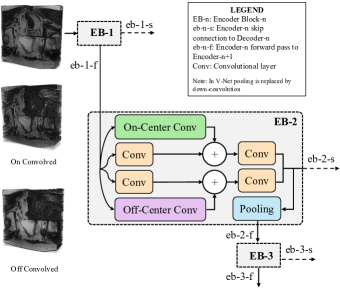
Figure 1: Extending U-Net-like architectures with the two 3D-OOCS inductive biases enhances their segmentation performance and their robustness to distribution shifts.

Since the success of AlexNet (Krizhevsky, Sutskever, and Hinton 2012), the biomedical-imaging community has investigated various CNN architectures as promising solutions to enhancing cancer-detection efficiency (Singh et al. 2020). U-Nets are a particular type of CNNs that were originally designed to work with small datasets and yield a highly accurate segmentation (Ronneberger, Fischer, and Brox 2015), first in 2D and later on in 3D medical imaging scenarios (Çiçek et al. 2016). The U-Net network has an encoder-decoder structure, where the encoder performs as a classification network based on annotated images. In contrast, the decoder is (loosely) a dual network that reconstructs the image from its discriminative features (low-dimensional feature space) in the original pixel-level space (high-dimensional features).

Inspired by the OOCS retinal circuitry and motivated by the significant efficacy of 2D OOCS in image-classification tasks (Babaiee et al. 2021), we investigated if the 3D OOCS extension can improve the accuracy and robustness of U-Net-like architectures. We first designed the 3D OOCS kernels and then modified the second encoder block of our U-Net baselines, with On and Off parallel pathways. Our experiments on prostate segmentation show that introducing OOCS blocks to a U-Net-like network not only improves its performance but also increases the network’s robustness to test-set distribution shifts, such as noise, blurring, and motion.

Related Work

Biologically Inspired Architectures

Vision models.

Originally, they were inspired by neuroscience and psychology. In the meantime, both neuroscience and artificial intelligence (AI), in particular computer vision, have enormously progressed. Nevertheless, most of today’s neural networks remained only loosely inspired by the visual system. The interaction between the fields has become less common, compared to the early age of AI, despite the importance of neuroscience in generating accelerating ideas for AI (Brooks et al. 2012; Hassabis et al. 2017).

2D OOCS kernels.

A recent paper introduced OOCS parallel pathways to CNNs and evaluated their effect in several image-classification and robustness scenarios (Babaiee et al. 2021). OOCS-CNNs outperformed the CNNs baselines in accuracy and surpassed state-of-the-art regularisation methods in unseen lighting conditions and noisy test sets (Babaiee et al. 2021). However, that paper only studied OOCS for image classification tasks and was limited to 2-dimensional natural image datasets. In this paper, we investigate 3D OOCS, which are beyond what exists in the human visual system. We also show the superior performance of networks incorporating 3D OOCS compared to their U-Net-like baselines in the 3D prostate segmentation task. Our experiments show that similar to the 2D version, 3D OOCS extensions significantly enhance accuracy and robustness.

Method

In this section we first show how we compute the 3D OOCS kernels. We then discuss how to extend a U-Net-like architecture with OOCS inductive biases.

3D OOCS Kernels

OOCS receptive fields are captured with a difference of two Gaussians (DoG) (Rodieck 1965). For 2D kernels, Equation (1) computes their center and surround weights (Petkov and Visser 2005; Kruizinga and Petkov 2000):

$$DoG_{\sigma,\gamma}(x,y)=\frac{A_{c}}{\gamma^{2}}\,e^{-\frac{x^{2}+y^{2}}{2\gamma^{2}\sigma^{2}}}-A_{s}\,e^{-\frac{x^{2}+y^{2}}{2\sigma^{2}}}$$ (1)

In Equation (1), $\gamma$ is the ratio of the radius of the center to the surround, $\gamma<1$, $\sigma$ is the variance of the Gaussian function, and $A_{c}$ and $A_{s}$ are the center and surround coefficients.

To construct 3D-OOCS kernels, the naive way would be to use Equation (1), and repeat the kernels in the third axis. However, this approach would result in a cylindrical center-surround structure, instead of a spherical one, with excitatory center, and an inhibitory surround. We therefore use a 3D DoG, with three parameters, extending the 2D version:

$$DoG_{\sigma,\gamma}(x,y,z)=\frac{A_{c}}{\gamma^{3}}\,e^{-\frac{x^{2}+y^{2}+z^{2}}{2\gamma^{2}\sigma^{2}}}-A_{s}\,e^{-\frac{x^{2}+y^{2}+z^{2}}{2\sigma^{2}}}$$ (2)

We set the absolute value of the sum of the negative and positive weights, to be equal to an arbitrary value $c\geq 1$. This ensures the proper balance between excitation and inhibition and the kernel weights will be large enough.

$$\iiint[DoG_{\sigma,\gamma}(x,y,z)]^{+}dxdydz=c,$$ (3)

$$\iiint[DoG_{\sigma,\gamma}(x,y,z)]^{-}dxdydz=-c$$ (4)

By setting the sum of negative and positive values to be equal, the coefficients $A_{c}$ and $A_{s}$ will be equal in the infinite continuous case. To show this, we can write the DoG equation in polar coordinates:

$$\int_{0}^{r_{s}}\!\!\!\!\int_{0}^{\pi}\!\!\!\!\int_{0}^{2\pi}\!\!\!\!\!\!r^{2}\,sin(\varphi)\,(\frac{A_{c}}{\gamma^{3}}\ e^{-\frac{r^{2}}{2\gamma^{2}\sigma^{2}}}-A_{s}\,e^{-\frac{r^{2}}{2\sigma^{2}}})d\theta d\varphi dr$$ (5)

Here $r$ is the radius of the central sphere. We can calculate the integral when $r\,{\to}\,\infty$, and by knowing the sum of positive and negative weights equals to zero, we have:

$$\frac{2\sqrt{2}\pi^{\frac{3}{2}}}{(\frac{1}{\sigma^{2}})^{\frac{3}{2}}}(A_{c}-A_{s})=0\ \ \Rightarrow\ \ A_{c}=A_{s}$$ (6)

Assuming that the values of the coefficients are still close enough in the finite discrete case as well, we can approximate the variance as follows:

$$\sigma\approx\frac{r}{\gamma}\sqrt{\frac{1-\gamma^{2}}{-6\ln{\gamma}}}$$ (7)

3D OOCS Encoder Blocks

We use Equation (2) to calculate the kernel weights for the On and Off (same equation, but with signs inverted) convolutions. Note that we only need to determine the kernel size, ratio of the radius of the center to surround, and sum of positive and negative values to compute the fixed kernels. Here we set $\gamma=\frac{2}{3}$ and $c=3$.

For a given input $\chi$, we calculate the On and Off responses by convolving $\chi$ with the computed kernels separately:

$$\begin{array}[]{c@{\ }c@{\ }l}\chi_{\rm On}[x,y,z]&=&(\chi*+DoG[r,\gamma,c])[x,y,z]\\[2.84526pt] \chi_{\rm Off}[x,y,z]&=&(\chi*-DoG[r,\gamma,c])[x,y,z]\end{array}$$ (8)

We extend a 3D U-Net-like segmentation network to a 3D OOCS network, by changing one of its primary encoder blocks, to a 3D OOCS encoder block, as shown in Figure 1. To this end, we first divide the convolution layers of the block into two parallel pathways, with half of the filters of the convolutions in the original layer, in each divided convolution, imitating the so-called On and Off pathways in the retina. We add the 3D On and Off convolved inputs of the block to the activation maps of the first convolution layers of the pathways. Finally, we concatenate the activation maps of the last layers on the pathways, resulting in the outputs with the same shapes as the outputs of the original block.

Experimental Evaluation

The proposed 3D OOCS filters are modular and independent of the network’s architecture. This allows them to be easily deployed to image segmentation tasks. All networks were evaluated on their ability to segment the prostate gland from MRIs. Owing to shape variability and poor tissue contrast in patient MRIs, prostate boundary delineation is challenging. The OOCS networks were compared against their respective counterparts by performing a rigorous robustness analysis.

U-Net-Like Networks

Along with the U-Net, we selected the Attention U-Net and the V-Net, as state-of-art U-Net benchmarks in the 3D medical image segmentation domain. These networks were selected based on the fact that they both introduced novel multi-view and multi-scale functions. The functions enhanced the receptive fields of the networks and reduced bottlenecks during computation, essentially shortening the time required to converge. All the standard networks were extended with 3D-OOCS filters of two different kernel sizes: $k=3$ and $k=5$, respectively. The new networks are called OOCS U-Net (k3), OOCS U-Net (k5), OOCS Attention U-Net (k3), OOCS Attention U-Net (k5), OOCS V-Net (k3), and OOCS V-Net (k5), respectively.

Parameter	Lower bound	Upper bound	Default value
$lr$	$10^{-6}$	0.1	$10^{-4}$
$\beta_{1}$	0.1	0.9	0.9
$dr$	0.0	0.7	0.5

Table 1: Hyper-parameter ranges used in the optimal-configuration search for the baselines and their extension.

Model Name	DSC	HSD(mm)
U-Net	$0.744\pm 0.24$	$33.777\pm 37.81$
OOCS U-Net (k3)	$0.798\pm 0.11$	$24.518\pm 12.46$
OOCS U-Net (k5)	$\mathbf{0.824\pm 0.07}$	$\mathbf{24.474\pm 12.48}$
V-Net	$0.792\pm 0.16$	$25.170\pm 22.91$
OOCS V-Net (k3)	$0.791\pm 0.13$	$26.488\pm 17.68$
OOCS V-Net (k5)	$\mathbf{0.825\pm 0.08}$	$\mathbf{21.471\pm 10.01}$
Attention U-Net	$0.824\pm 0.09$	$27.822\pm 14.64$
OOCS Att. U-Net (k3)	$\mathbf{0.845\pm 0.07}$	$24.106\pm 14.70$
OOCS Att. U-Net (k5)	$0.835\pm 0.11$	$\mathbf{23.531\pm 14.89}$

Table 2: Segmentation test results of different U-Nets and their OOCS extensions.

Dataset and Pre-Processing

The Medical Segmentation Decathlon (MSD)(Simpson et al. 2019) - prostate dataset comprises of 48 (training =32, testing =16) multimodal (T2, ADC) 3D MRI samples. However, the ground-truth labels for the testing images are not publicly accessible, and therefore, we implemented a 5-fold cross-validation. The available dataset (n=32) was split into training (80%) and testing (20%) samples for each fold (for details, please refer to the supplements file). Since the T2-weighted volumes provide most of the necessary anatomical information, and the ADC modality is often used for tumour characterization/segmentation, we only considered the T2-weighted modality for our experiments. Furthermore, the ground-truth labels of the original dataset are separated into annotations of the central prostate gland and the peripheral zone. We combined the two target regions into one such that the networks could learn binary image segmentations. The MRI scans and the ground truth labels were resampled to ($0.6$, $0.6$, $0.6$) voxel spacings with tri-linear and nearest-neighbor interpolation techniques, respectively. The resampling was done to increase the slice thickness and facilitate the smooth functioning of the networks without any alteration in their original architecture.

Model Name	$\sigma=2$	$\sigma=3$	$\sigma=3.5$
U-Net	$0.483\pm 0.36$	$0.242\pm 0.33$	$0.269\pm 0.33$
OOCS U-Net (k3)	$0.378\pm 0.36$	$0.311\pm 0.37$	$0.257\pm 0.34$
OOCS U-Net (k5)	$0.477\pm 0.34$	$0.344\pm 0.39$	$0.293\pm 0.34$
V-Net	$0.489\pm 0.38$	$0.243\pm 0.35$	$0.365\pm 0.37$
OOCS V-Net (k3)	$0.354\pm 0.36$	$0.312\pm 0.39$	$0.252\pm 0.34$
OOCS V-Net (k5)	$0.461\pm 0.37$	$0.341\pm 0.40$	$0.264\pm 0.36$
Attention U-Net	$0.688\pm 0.23$	$0.503\pm 0.28$	$\mathbf{0.533\pm 0.28}$
OOCS Att. U-Net (k3)	$0.691\pm 0.16$	$0.467\pm 0.35$	$0.427\pm 0.34$
OOCS Att. U-Net (k5)	$\mathbf{0.773\pm 0.11}$	$\mathbf{0.535\pm 0.33}$	$0.528\pm 0.32$

Table 3: Robustness of U-Net variants against Gaussian Blur Noise (using DSC metric).

Model Name	$\sigma=30$	$\sigma=45$	$\sigma=60$
U-Net	$0.737\pm 0.23$	$0.640\pm 0.29$	$0.458\pm 0.38$
OOCS U-Net (k3)	$0.792\pm 0.12$	$0.780\pm 0.13$	$0.746\pm 0.18$
OOCS U-Net (k5)	$0.822\pm 0.07$	$0.816\pm 0.07$	$0.807\pm 0.08$
V-Net	$0.677\pm 0.30$	$0.633\pm 0.30$	$0.533\pm 0.34$
OOCS V-Net (k3)	$0.774\pm 0.17$	$0.714\pm 0.24$	$0.630\pm 0.29$
OOCS V-Net (k5)	$0.824\pm 0.08$	$0.822\pm 0.08$	$\mathbf{0.822\pm 0.09}$
Attention U-Net	$0.795\pm 0.15$	$0.715\pm 0.26$	$0.614\pm 0.32$
OOCS Att. U-Net (k3)	$\mathbf{0.837\pm 0.08}$	$0.795\pm 0.13$	$0.697\pm 0.25$
OOCS Att. U-Net (k5)	$0.833\pm 0.11$	$\mathbf{0.827\pm 0.12}$	$0.813\pm 0.13$

Table 4: Robustness of U-Net variants against Random Gaussian Noise (using DSC metric).

Model Name	$transform\#=5$	$transform\#=8$	$transform\#=10$
U-Net	$0.629\pm 0.26$	$0.608\pm 0.28$	$0.564\pm 0.30$
OOCS U-Net (k3)	$0.484\pm 0.24$	$0.451\pm 0.32$	$0.506\pm 0.31$
OOCS U-Net (k5)	$0.668\pm 0.10$	$0.592\pm 0.26$	$0.613\pm 0.24$
V-Net	$0.619\pm 0.30$	$0.674\pm 0.26$	$0.591\pm 0.32$
OOCS V-Net (k3)	$0.610\pm 0.28$	$0.613\pm 0.29$	$0.634\pm 0.24$
OOCS V-Net (k5)	$0.757\pm 0.08$	$0.669\pm 0.26$	$0.659\pm 0.23$
Attention U-Net	$0.764\pm 0.14$	$0.806\pm 0.09$	$\mathbf{0.775\pm 0.12}$
OOCS Att. U-Net (k3)	$\mathbf{0.788\pm 0.07}$	$\mathbf{0.821\pm 0.07}$	$0.770\pm 0.11$
OOCS Att. U-Net (k5)	$0.771\pm 0.10$	$0.800\pm 0.09$	$0.747\pm 0.15$

Table 5: Robustness of U-Net variants against Motion Noise (using DSC metric).

Furthermore, the 3D images were cropped during the experiments to a selected shape of $160\,{\times}\,160\,{\times}\,64$ voxels per patch. For a given batch of samples, the intensity values of the MRIs were linearly scaled using a standard (z-score) normalization. Since the dataset is made up of a small number of volumes, the data pipeline carried out augmentations such as axial flips, elastic deformations, random crops, and affine transformations (scaling, rotation, and translation).

Implementation

A combination of two-loss functions: Binary Cross-Entropy loss (L_BCE) and Sørensen-Dice Loss (L_dice) (Sudre et al. 2017) called BCE-dice loss (L_BCE-dice) was used to train the models. As demonstrated experimentally, this compound loss is defined over all semantic classes and is less sensitive to class imbalance (Ma et al. 2021). The models were evaluated based on two metrics: DSC and symmetric Hausdorff Distance (HSD). They were chosen because they exhibit low overall biases in 3D medical image segmentation tasks (Taha and Hanbury 2015). We used the Adam optimization algorithm along with a cosine-annealing learning rate scheduler (Kingma and Ba 2015; Loshchilov and Hutter 2017) throughout all the experiments. A batch normalization layer was placed after every convolution layer, to accelerate the speed of the experiments, and also serve as a regularizer (Ioffe and Szegedy 2015). All the networks were implemented in PyTorch (Paszke et al. 2019). We ran our experiments without data-parallelism on the NVIDIA Titan RTX with 24 GB memory. The gradient updates were evaluated with a batch size of two samples.

Training

Individual network hyper-parameter searches were done with MRIs of fold-1. This ensured that all models achieved their peak performance, and therefore, a fair and objective comparison was conducted among all networks. The search space, as described in Table 1, was used to fine-tune the learning rate ($lr$), Adam’s momentum ($\beta_{1}$), and the dropout rate ($dr$). Please see the supplements for the table of the tuned parameters found for each network. After finding the optimal hyper-parameters for a network, four additional models of the same network were trained using the four remaining cross-validation folds, and the fine-tuned values of $lr$, $\beta_{1}$ and $dr$. This kind of training was repeated for all the networks.

Results

Testing

The testing of the networks was done employing the sliding window approach where the window size equals the patch size used during training. The average DSC and HSD of all the networks are listed in the Table 2. Here, it is evident that the OOCS-Attention-U-Net variations performed best. In addition, the OOCS extensions have consistently outperformed their original counterparts in most instances. The superior performance of the OOCS models showcases the ability of the inductive bias in the OOCS filters to delineate prostate contours effectively.

Robustness Evaluation

To examine the robustness of the models, we introduced three types of noise: Gaussian blur, random Gaussian noise, and motion transform (simulating artifacts due to patient movement during acquisition), into the test volumes. In case of blurring, the average DSCs of the models decreased with the increase in standard deviation ($\sigma$) of the noise level. This behaviour was anticipated since higher deviations produced samples with large perturbations. On the other hand, the prostate predictions of the OOCS models were considerably stable across both random Gaussian and motion artifacts. This demonstrates that the OOCS-extensions have a lower variance when compared to the benchmark networks on complex test sets and in the presence of outliers. Finally, the OOCS-Attention-U-Net (k5) significantly outperforms all U-Net-like benchmarks and their extensions. Tables 3, 4 and  5 summarise the results of the robustness evaluation of the OOCS models and the state-of-the-art models. Please refer to the supplement for the illustration of a few of the examples with noise information, along with the predictions of the benchmark and the OOCS Attention U-Net (k5) models, respectively.

Conclusion

We expanded the On-Off center-surround retinal receptive fields to 3D kernels, and proposed a straightforward method to calculate the kernel weights. We designed OOCS encoder blocks using these fixed and pre-computed kernels as edge detection inductive biases, with On and Off parallel pathways similar to the ganglion pathways in the visual system. Our proposed 3D OOCS encoder block does not increase the number of training parameters of the networks and requires minimal computational overhead. Moreover, it is effortless to equip any UNet-like network with these encoder blocks. Our experiments on prostate segmentation tasks with our baseline networks and their OOCS extensions show notable enhancements in the performance of the OOCS-equipped networks, thus making 3D-OOCS a favorable method to achieve accurate results in 3D medical image segmentation tasks. Furthermore, our robustness experiments demonstrate the superior performance of OOCS extended networks. Robustness to distribution shifts is a crucial attribute of any deep neural network, and it is of even higher importance for networks used in critical domains like bio-medical tasks.

Code and Data Availability

All code and data are included in https://github.com/Shrajan/AAAI-2022.

References

- Babaiee et al. (2021) Babaiee, Z.; Hasani, R.; Lechner, M.; Rus, D.; and Grosu, R. 2021. On-Off Center-Surround Receptive Fields for Accurate and Robust Image Classification. In Meila, M.; and Zhang, T., eds., Proceedings of the 38th International Conference on Machine Learning, volume 139 of Proceedings of Machine Learning Research, 478–489. PMLR.
- Brooks et al. (2012) Brooks, R.; Hassabis, D.; Bray, D.; and Shashua, A. 2012. Turing centenary: Is the brain a good model for machine intelligence? Nature, 482: 462–3.
- Çiçek et al. (2016) Çiçek, Ö.; Abdulkadir, A.; Lienkamp, S. S.; Brox, T.; and Ronneberger, O. 2016. 3D U-Net: Learning Dense Volumetric Segmentation from Sparse Annotation. CoRR, abs/1606.06650.
- Goldenberg, Nir, and Salcudean (2019) Goldenberg, S. L.; Nir, G.; and Salcudean, S. E. 2019. A new era: artificial intelligence and machine learning in prostate cancer. Nature Reviews Urology, 16(7): 391–403.
- Hassabis et al. (2017) Hassabis, D.; Kumaran, D.; Summerfield, C.; and Botvinick, M. 2017. Neuroscience-Inspired Artificial Intelligence. Neuron, 95(2): 245–258.
- Ioffe and Szegedy (2015) Ioffe, S.; and Szegedy, C. 2015. Batch Normalization: Accelerating Deep Network Training by Reducing Internal Covariate Shift. CoRR, abs/1502.03167.
- Kingma and Ba (2015) Kingma, D. P.; and Ba, J. 2015. Adam: A Method for Stochastic Optimization. In Bengio, Y.; and LeCun, Y., eds., 3rd International Conference on Learning Representations, ICLR 2015, San Diego, CA, USA, May 7-9, 2015, Conference Track Proceedings.
- Krizhevsky, Sutskever, and Hinton (2012) Krizhevsky, A.; Sutskever, I.; and Hinton, G. E. 2012. ImageNet Classification with Deep Convolutional Neural Networks. In Pereira, F.; Burges, C. J. C.; Bottou, L.; and Weinberger, K. Q., eds., Advances in Neural Information Processing Systems, volume 25. Curran Associates, Inc.
- Kruizinga and Petkov (2000) Kruizinga, P.; and Petkov, N. 2000. Computational Model of Dot-Pattern Selective Cells. Biological Cybernetics, 83(4): 313–325.
- Loshchilov and Hutter (2017) Loshchilov, I.; and Hutter, F. 2017. Fixing Weight Decay Regularization in Adam. CoRR, abs/1711.05101.
- Ma et al. (2021) Ma, J.; Chen, J.; Ng, M.; Huang, R.; Li, Y.; Li, C.; Yang, X.; and Martel, A. L. 2021. Loss odyssey in medical image segmentation. Medical Image Analysis, 71: 102035.
- Paszke et al. (2019) Paszke, A.; Gross, S.; Massa, F.; Lerer, A.; Bradbury, J.; Chanan, G.; Killeen, T.; Lin, Z.; Gimelshein, N.; Antiga, L.; Desmaison, A.; Kopf, A.; Yang, E.; DeVito, Z.; Raison, M.; Tejani, A.; Chilamkurthy, S.; Steiner, B.; Fang, L.; Bai, J.; and Chintala, S. 2019. PyTorch: An Imperative Style, High-Performance Deep Learning Library. In Wallach, H.; Larochelle, H.; Beygelzimer, A.; d'Alché-Buc, F.; Fox, E.; and Garnett, R., eds., Advances in Neural Information Processing Systems 32, 8024–8035. Curran Associates, Inc.
- Petkov and Visser (2005) Petkov, N.; and Visser, W. 2005. Modifications of Center-Surround, Spot Detection and Dot-Pattern Selective Operators. Technical Report 2005-9-01, Institute of Mathematics and Computing Science, University of Groningen, Netherlands.
- Rischke et al. (2013) Rischke, H. C.; Nestle, U.; Fechter, T.; Doll, C.; Volegova-Neher, N.; Henne, K.; Scholber, J.; Knippen, S.; Kirste, S.; Grosu, A. L.; and Jilg, C. A. 2013. 3 Tesla multiparametric MRI for GTV-definition of Dominant Intraprostatic Lesions in patients with Prostate Cancer–an interobserver variability study. Radiat Oncol, 8: 183.
- Rodieck (1965) Rodieck, R. 1965. Quantitative Analysis of Cat Retinal Ganglion Cell Response to Visual Stimuli. Vision Research, 5(12): 583–601.
- Ronneberger, Fischer, and Brox (2015) Ronneberger, O.; Fischer, P.; and Brox, T. 2015. U-Net: Convolutional Networks for Biomedical Image Segmentation. In Navab, N.; Hornegger, J.; Wells, W. M.; and Frangi, A. F., eds., Medical Image Computing and Computer-Assisted Intervention – MICCAI 2015, 234–241. Cham: Springer International Publishing. ISBN 978-3-319-24574-4.
- Simpson et al. (2019) Simpson, A. L.; Antonelli, M.; Bakas, S.; Bilello, M.; Farahani, K.; van Ginneken, B.; Kopp-Schneider, A.; Landman, B. A.; Litjens, G.; Menze, B. H.; Ronneberger, O.; Summers, R. M.; Bilic, P.; Christ, P. F.; Do, R. K. G.; Gollub, M.; Golia-Pernicka, J.; Heckers, S.; Jarnagin, W. R.; McHugo, M.; Napel, S.; Vorontsov, E.; Maier-Hein, L.; and Cardoso, M. J. 2019. A large annotated medical image dataset for the development and evaluation of segmentation algorithms. CoRR, abs/1902.09063.
- Singh et al. (2020) Singh, S. P.; Wang, L.; Gupta, S.; Goli, H.; Padmanabhan, P.; and Gulyás, B. 2020. 3D Deep Learning on Medical Images: A Review. Sensors, 20(18).
- Spohn et al. (2021) Spohn, S. K.; Bettermann, A. S.; Bamberg, F.; Benndorf, M.; Mix, M.; Nicolay, N. H.; Fechter, T.; Hölscher, T.; Grosu, R.; Chiti, A.; Grosu, A. L.; and Zamboglou, C. 2021. Radiomics in prostate cancer imaging for a personalized treatment approach - current aspects of methodology and a systematic review on validated studies. Theranostics, 11: 8027–8042.
- Steenbergen et al. (2015) Steenbergen, P.; Haustermans, K.; Lerut, E.; Oyen, R.; De Wever, L.; Van den Bergh, L.; Kerkmeijer, L. G.; Pameijer, F. A.; Veldhuis, W. B.; van der Voort van Zyp, J. R.; Pos, F. J.; Heijmink, S. W.; Kalisvaart, R.; Teertstra, H. J.; Dinh, C. V.; Ghobadi, G.; and van der Heide, U. A. 2015. Prostate tumor delineation using multiparametric magnetic resonance imaging: Inter-observer variability and pathology validation. Radiother Oncol, 115(2): 186–190.
- Sudre et al. (2017) Sudre, C. H.; Li, W.; Vercauteren, T.; Ourselin, S.; and Cardoso, M. J. 2017. Generalised Dice overlap as a deep learning loss function for highly unbalanced segmentations. CoRR, 10553: 240–248.
- Taha and Hanbury (2015) Taha, A. A.; and Hanbury, A. 2015. Metrics for evaluating 3D medical image segmentation: analysis, selection, and tool. BMC Medical Imaging, 15(1): 29.