First post-Newtonian correction to gravitational waves produced by compact binaries:
How to compute relativistic corrections to gravitational waves using Feynman diagrams

See pages 2 of figures/CoverAndFrontPage.pdf

Abstract

The purpose of this thesis is to calculate the relativistic correction to the gravitational wave s produced by compact binaries in the inspiral phase. The correction is up to the next to leading order, the so-called first post-Newtonian order (1PN), which are correctional terms proportional to $(v/c)^{2}$ compared to leading order, Newtonian, terms.

These corrections are well known in the literature, even going beyond the first order corrections, so why is it computed again here? In later years, an alternative approach for computing these terms using effective field theory has emerged. This thesis investigates this approach by replicating it, and attempts to make this approach more accessible to those not familiar with effective field theories.

It has been claimed that this approach greatly simplifies the complicated calculations of gravitational wave forms, and even provides the required intuition for ‘physical understanding’. By this master student that was found not to be entirely correct. The calculations were made easier for those with a rich background in quantum field theory , but for those who are not well acquainted with quantum field theory this was not the case.

It was, however, found to be a worthwhile method as a means for deepening one’s understanding of gravity, and might provide a shorter route for some alternative theories of gravity to testable predictions.

Sammendrag

Hensikten med denne oppgaven er å beregne den relativistiske korreksjonen til gravitasjonsbølger som er produsert av kompakte binærsystemer i spiral-fall fasen. Korreksjonene er av den såkalte første post-Newtonske orden (1PN), som er korreksjonstermer proporsjonal med $(v/c)^{2}$ sammenlignet med ledende, Newtonske, termerene.

Disse korreksjonene er velkjente i litteraturen, og går til og med utover korreksjonene av første orden, så hvorfor blir de beregnet igjen her? I nyere tid har en alternativ tilnærming for å beregne disse størrelsene ved hjelp av effektiv feltteori dukket opp. Denne oppgaven undersøker tilnærmingen ved å reprodusere dem, og prøver å gjøre metoden mer tilgjengelig for de som ikke er kjent med effektive feltteorier.

Det har blitt hevdet at beregningen av gravitasjonsbølgeformer kan gjøres mye enklere ved å bruke denne tilnærmingen, og til og med gir den nødvendige intuisjonen for ‘fysisk forståelse’. Ifølge denne masterstudenten er ikke dette helt riktig. Beregningene ble gjort enklere for de med en spesialisert bakgrunn i kvantefeltteori, og for de som er mindre kjent med kvantefeltteori var dette ikke tilfelle.

Det ble imidlertid funnet å være en verdifull metode som et middel for å utdype forståelsen av tyngdekraften, og kan gi en kortere rute for noen alternative teorier for gravitasjon til testbare forutsigelser.

Foreword

This document is for all intents and purposes my master’s thesis, but it deviates to some degree from the document that was handed in for the examination.

The reason for this is that this document has been updated based on helpful comments from the examiner, Professor David Fonseca Mota, with additional clarifications and purging of typos. This will hopefully make this document better suited than the original thesis for those who want to use it as an introduction to the use of field theories in gravitational wave physics.

The original thesis can be found at NTNU’s digital thesis archive at https://hdl.handle.net/11250/2785590

Contents

1. 1 Introduction
   1. 1.1 Binary inspirals and gravitational waves
   2. 1.2 Structure of this thesis
   3. 1.3 Why effective field theory?
   4. 1.4 Notation
2. 2 The gravitational waveform
   1. 2.1 Setting up the equation for the gravitational waveform
      1. 2.1.1 What is a waveform?
      2. 2.1.2 Time evolution of orbital energy
   2. 2.2 Computing the waveform
      1. 2.2.1 Computing the waveform as a function of time
      2. 2.2.2 Computing the Fourier transform of the waveform
3. 3 Gravity as a gauge theory
   1. 3.1 Background
   2. 3.2 Fierz-Pauli Lagrangian
      1. 3.2.1 Deriving the graviton Lagrangian
      2. 3.2.2 The equation of motion and gauge condition
   3. 3.3 Solutions of the graviton field
      1. 3.3.1 Gravitational waves in vacuum, and their polarization
      2. 3.3.2 Source of gravitational waves
      3. 5.2.2 Next to leading order term, the octupole moment
      4. 5.2.3 Next to leading order term, the current quadrupole moment
      5. 5.2.4 Next to leading order term, the quadrupole moment corrections
      6. 5.2.5 The total 1PN energy flux
4. 6 Discussion and conclusion
5. A Solution of the wave equation
6. B Equivalent one body problem and mass term manipulation
   1. B.1 Rewriting to the equivalent one body problem
   2. B.2 Mass term manipulation
7. C Trigonometric identities

List of Figures

1. 1.1 Phases of binary evolution.
2. 2.1 Waveform of GW produced by binary systems.
3. (a) Waveform including (red) and excluding (blue) first order corrections. The waveform was plotted for values matching those of Table 1 of [1]. The plot depicts the waveform as seen in the detector frame, i.e. cosmologically redshifted.
4. (b) Data and model by LIGO for GW150914, published in [1].
5. B.1 Diagram of a binary system.

Acronyms

BH

black hole

EFT

effective field theory

EoM

equation of motion

FP

Fierz-Pauli

gf

gauge fixing term

GR

general relativity

GW

gravitational wave

LHS

left hand side

LIGO

Laser Interferometer Gravitational-Wave Observatory

NS

neutron star

PN

post-Newtonian

pp

point particle

QFT

quantum field theory

RHS

right hand side

SPA

stationary phase approximation

STF

symmetric trace free

TT

transverse-traceless

Glossary

two body problem

Name of the physics problem of describing how a system consisting of two bodies (usually taken to be point particles) evolve in time, given they only interact with each other. For $r^{-1}$ potentials the two body problem generally has the solution of conic sections [2]

black hole

A region of space-time curved to the point that no matter or radiation can escape. Usually taken to be a gravitationally collapsed star

Einstein’s field equations

The equations of motion resulting from the Einstein-Hilbert action which dictates the dynamics of space-time. Coupled to a matter source it reads $R\ind{{}_{\mu\nu}}-\frac{1}{2}Rg\ind{{}_{\mu\nu}}=\frac{8\pi G}{c^{4}}T\ind{{}_{\mu\nu}}$

Einstein-Hilbert action

Einstein-Hilbert action is the action which when extremized generates the , i.e. the action which governs $S_{\text{}}=\frac{c^{4}}{16\pi G}\int R\sqrt{-g}\differential[4]{x}$

field theorist

Physicists using fields on a static background space-time to model physical effects like forces and particles. In this thesis especially those who use fields to model gravity

GW150914

The gravitational wave event which occurred 14/09/2015. The first event by [1]

quasi-stable circular orbit

Approximating the inspiral as circular orbits with gradually falling radii. The change in radius is negligible unless viewed over several periods

quantum field theory

The theory of fields endowed with quantum properties that can be used to describe forces and matter

relativist

Physicists using a geometrical interpretation of gravity, following in the footsteps of Einstein

Chapter 1 Introduction

1.1 Binary inspirals and gravitational waves

On the 14^th of September 2015 the world was shocked, ever so slightly. So slightly in fact that the only reason we know about it is thanks to the effort of the Laser Interferometer Gravitational-Wave Observatory (LIGO), who measured this faint strain in their detectors. After careful testing and retesting, LIGO published their results on the 11^th of February 2016 [1]. They concluded that the event, called GW150914, was a gravitational wave (GW)produced by the merger of two black holes, and was the first directly detected gravitational wave event in human history.

With the announcement of the historic detection of GW150914 came promises of a new era of astronomy, now equipped with a brand new type of data to constrain astronomical theories. Popular science lectures and books were given and written, and at the height of this hype I started my bachelor’s degree in physics. Fascinated by these mysterious waves I wanted to learn more about them, and when the time came to pick a topic for my master’s thesis I requested to work on gravitational wave s.

My supervisor and I decided to work on relativistic corrections to the binary inspiral, using field theoretical methods. To date, all confirmed GW events are thought to be produced by compact binaries. A compact object is a black hole (BH)or neutron star (NS), and a compact binary is a system consisting of two compact objects. When compact objects revolve around each other they produce so called gravitational wave s which dissipate orbital energy from the system. As a result the compact objects fall toward each other, and in the end collide and merge together.

The problem with compact binaries is that they are too heavy and fall too close to each other, making the gravitational interaction too strong to be adequately described by Newton’s law of gravity. Although the two body problem has a general solution in Newtonian mechanics, there is no known equivalent solution for the two body problem in general relativity, only the one body problem. To combat this issue, researchers have followed one of two approaches.

1. Solve the full, non-linear, Einstein’s field equations numerically for the binary system in question.

2. Use an approximate, analytical, solution and perturbatively expand it to account for relativistic corrections.

This thesis will focus on analytical approximations. With numerical simulations one obtains a picture of the dynamics at an arguably very high accuracy, but due to the complexity of Einstein’s field equations this is computationally costly, i.e. takes a lot of time and computing power. Furthermore, analytical expressions provide information about important quantities and intuition about the most important physical effects at play, that one simply does not gain from computer simulations.

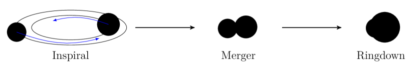
Figure 1.1: The evolution of compact binaries in three phases.

In order to expand an analytical solution relativistically one first needs an approximate solution to expand. For this it is useful to divide the evolution of the compact binary into three phases, see Figure 1.1. The first phase is called the inspiral phase. Here the compact objects orbit each other at a distance, gradually falling closer together due to the emission of gravitational wave s. Once the bodies are so close that a collision is imminent (typically when they ‘touch’ or form a common event horizon) the system becomes highly non-linear, and enters the so-called merger phase. After the two objects have merged into one, the system enters the ringdown phase, in which the system can be described as a one body problem, but with remnant asymmetries from the merger. Typically, the merged object’s asymmetries oscillate around the Kerr solution and gradually dampen down, hence the name ringdown.

This is a useful division of the binary evolution as the different phases lend themselves to different approximations. The first phase, the inspiral, can be approximated as Keplerian orbits since the leading order term in the equations of motion is the Newtonian law of gravitation. The last phase can be approximated as a Schwarzschild or Kerr solution with perturbations. The merger phase is sandwiched between these two widely different approximations and is dominated by non-linear effects. Thus the merger phase has no good analytical approximation and must be simulated numerically.

In this thesis I will work with the analytical approximation of the inspiral phase.

1.2 Structure of this thesis

As we will see in Chapter 3 the frequency of the gravitational wave s produced by compact binaries are directly dependent on the frequency at which the source oscillates, which is found to be inverse proportional to the total mass of the binary raised to the $5/8$ths power: $\omega_{\text{source}}\propto M^{-5/8}$ (see equation (2.18)). Therefore, the waveform of GW s measured here on Earth provides information about the dynamics of the binary which produced it, and can be compared with the predicted dynamics according to general relativity. This is why GW observation is a precise tool for constraining theories of gravity.

To motivate these computations, Chapter 2 starts off by computing the waveform, using results from following chapters. Then in Chapter 3 an alternative path to gravity is presented, that of a gauge field theory on a static space-time background. It is demonstrated to recover the main results of standard linearized gravity, which is the Einstein’s field equations expanded to linear order in metric perturbations over flat space-time. In LABEL:chap:energy and LABEL:chap:flux the main results needed to compute the waveform in Chapter 2 are derived, using the effective field theory (EFT)based on the material presented in Chapter 3. Then the thesis ends with Chapter 6, which is concluding remarks on the effective field theory approach to gravitational waves.

This is a form of top down approach, starting with the final result (the waveform) and working back to the fundamental assumptions behind it. This structure has been chosen because of the large amount of laboursome calculations leading to the gravitational wave form, and it will hopefully provide the overview needed to understand the motivation for each calculation as it appears.

1.3 Why effective field theory?

In 2006, [3] wrote a paper showing how the gravitational wave form could systematically be calculated to any post-Newtonian (PN)order using EFT formalism. Post-Newtonian expansion is ordering results like energy, the equation of motion, radiated energy flux, velocity, etc. as the Newtonian result plus relativistic corrections, usually expanded in factors of $v/c$.

E.g.

$$E=E_{\text{Newt}}\left[1+\sum_{i=2}^{\infty}E_{i}\left(\frac{v}{c}\right)^{i}\right].$$ (1.1)

Here $E_{\text{Newt}}\cdot E_{i}\left(\frac{v}{c}\right)^{i}$ would be the $\frac{i}{2}$PN term of the energy. This scaling as half the $v/c$ power is chosen to represent the PN order such that the leading order correction is $1$PN.

In this thesis, working with fields on a non-dynamic, flat, space-time will be referred to as field theory, or the approach of field theorists, like Goldberger. This is supposed to be contrary to traditional geometrical theories of gravity, in the spirit of Einstein, which will be referred to as the approach of relativists. By any normal definition however, general relativity and its interpretation by relativists, is a field theory. But they work with dynamical space-times, making it conceptually and mathematically quite differently formulated. Therefore, these constructed labels of field theorists and relativists will be employed in this thesis to emphasize the difference in approach.

Formulating the computations in the language of field theorists, Goldberger and Rothstein unlocked all tools, tricks, and language usually reserved for quantum field theory (QFT). Since then, this approach has been argued by field theorists to be easier and faster than the traditional relativist approach, and has thus far produced results up to the 6th PN order [4, 5] and a detailed description up to the 5th order [6, 7, 8, 9, 10]. One of these field theorists, R. Porto, has even claimed [11]

“[…] that adopting an EFT framework, when possible, greatly simplifies the computations and provides the required intuition for ‘physical understanding’.”

My supervisor, a self-proclaimed relativist, got curious, and wondered just how easy the effective field theory approach would make the computation. Therefore, he asked me if I would try to go through these computations, to test if they made the computation manageable even for master’s students. My comments on Porto’s claim are given in the discussion of Chapter 6.

With verifying or refuting Porto’s claim as the ultimate goal of this thesis, it is mostly written as a relativist’s guide to a field theorists’ approach to gravitational wave s. It should also be useful for those with a field theoretical background who wish to understand how Feynman diagrams can be used in classical gravity, and gravitational wave physics.

1.4 Notation

This thesis uses the mostly positive flat space-time metric

$$\eta\ind{{}_{\mu\nu}}=\begin{pmatrix}-1&0&0&0\\ 0&1&0&0\\ 0&0&1&0\\ 0&0&0&1\end{pmatrix}$$ Flat metric

Four-vectors are written with Greek letter indices, and spatial vectors with Latin letter indices. The Einstein summation convention applies.

$$x\ind{{}^{\mu}}=\MixVec{x\ind{{}^{0}}}{\tvec{x}}=\MixVec{ct}$$ Four-vector

$$\partial\ind{{}_{\mu}}=\partialderivative{x\ind{{}^{\mu}}}=\MixVec{\frac{1}{c}\partial_{t}}{\nabla}$$ Four-gradienet

$$\differential[4]{x}=\differential{x\ind{{}^{0}}}\differential[3]{x}=c\differential{t}\differential[3]{x}$$ Integration volume of space-time

Notably, the action is defined as

$$S=\int\differential{t}L=\int\frac{\differential[4]{x}}{c}\L,$$

with $L$ and $\L$ being the Lagrangian, and Lagrangian density, respectively.

These tensor index notations are also used.

$$T\ind{{}_{[\mu\nu]}}\equiv\frac{1}{2!}\left(T\ind{{}_{\mu\nu}}-T\ind{{}_{\nu\mu}}\right)=A\ind{{}_{\mu\nu}}$$ Antisymmetrizing operation

$$T\ind{{}_{\{\mu\nu\}}}\equiv\frac{1}{2!}\left(T\ind{{}_{\mu\nu}}+T\ind{{}_{\nu\mu}}\right)=S\ind{{}_{\mu\nu}}$$ Symmetrizing operation

$$T=T\ind{{}_{\alpha}^{\alpha}}=\eta\ind{{}_{\alpha\beta}}T\ind{{}^{\alpha\beta}}$$ Trace of tensor

$$T\ind{{}_{\mu\nu,\alpha}}=\partial\ind{{}_{\alpha}}T\ind{{}_{\mu\nu}}$$ Partial derivative

$$T\ind{{}_{\mu\nu,\alpha}^{\alpha}}=\partial\ind{{}_{\alpha}}\partial\ind{{}^{\alpha}}T\ind{{}_{\mu\nu}}=\dalembertian T\ind{{}_{\mu\nu}}$$ d’Alembertian operator

$$\bar{T}\ind{{}_{\mu\nu}}=\frac{1}{2}\left(T\ind{{}_{\mu\nu}}+T\ind{{}_{\nu\mu}}-T\ind{{}^{\sigma}_{\sigma}}\eta\ind{{}_{\mu\nu}}\right)$$ Bar operator

Colons will also appear in indices, but these have no mathematical meaning. Colons are simply used to separate pairs of indices that have distinct roles. E.g. could $T\ind{{}^{\mu\nu}}x\ind{{}^{\lambda}}\equiv S\ind{{}^{\mu\nu:\lambda}}$.

Lastly, the Fourier transform, and inverse Fourier transform are defined by

$$F(x) =\int\frac{\differential[4]{k}}{(2\pi)^{4}}\tilde{F}(k)e^{ik\ind{{}_{\sigma}}x\ind{{}^{\sigma}}},$$

$$\tilde{F}(k) =\int\differential[4]{x}F(x)e^{-ik\ind{{}_{\sigma}}x\ind{{}^{\sigma}}}.$$

Chapter 2 The gravitational waveform

In this chapter the gravitational wave form will be computed, both in the time domain (2.19) and in the frequency domain (2.27).

The computation follows standard methods, like presented in [12].

2.1 Setting up the equation for the gravitational waveform

2.1.1 What is a waveform?

As inferred by the name, gravitational wave s are waves, which is to say they are solutions of the wave equation.

$$\left(-\partialderivative[2]{(ct)}+\nabla^{2}\right)h\ind{{}_{\mu\nu}}=\partial\ind{{}_{\alpha}}\partial\ind{{}^{\alpha}}h\ind{{}_{\mu\nu}}\equiv\dalembertian h\ind{{}_{\mu\nu}}=0.$$ (2.1)

Here the d’Alembert operator, also called the d’Alembertian, $\dalembertian$ has been defined, which is the operator of the wave equation.

A simple solution to equation (2.1) is $h\ind{{}_{\mu\nu}}=\epsilon\ind{{}_{\mu\nu}}e^{-ik\ind{{}_{\sigma}}x\ind{{}^{\sigma}}}$, with $k\ind{{}_{\mu}}k\ind{{}^{\mu}}=-k_{0}^{2}+\tvec{k}^{2}=0$, and where $\epsilon\ind{{}_{\mu\nu}}$ is some $x\ind{{}^{\mu}}$-independent tensor structure. The exponential is a plane wave solution, according to Euler’s formula (C.1).

Gravitational waves are rank two tensors, which means they have two indices and therefore $4\times 4=16$ components. It is also symmetric in these two indices: $h\ind{{}_{\mu\nu}}=h\ind{{}_{\nu\mu}}$, which means that only $10$ of these components are independent. The reason gravitational waves are rank two tensors follows in the relativist s’ approach because $h\ind{{}_{\mu\nu}}$ is a perturbation of the metric $g\ind{{}_{\mu\nu}}=\eta\ind{{}_{\mu\nu}}+h\ind{{}_{\mu\nu}}$, where $\eta\ind{{}_{\mu\nu}}$ is the flat space-time metric. In the field theorists’ approach it is because gravity is the effect of a massless spin two field. $\epsilon\ind{{}_{\mu\nu}}$ is the polarization tensor of GW s, and since it is a massless field it only has two independent polarizations. Gravitational waves are transverse, and thus $\epsilon\ind{{}_{ij}}k\ind{{}^{j}}=0$, i.e. the amplitude direction given by the polarization is orthogonal to the direction of propagation $\tvec{k}$.

To solve the wave equation, the wave four-vector had to be null-like. This implies further that the wave itself must travel at the speed of light, $v=\partialderivative{\omega}{\absolutevalue{\tvec{k}}}=\partialderivative{ck_{0}}{\absolutevalue{\tvec{k}}}=c$. This is also a consequence of $h\ind{{}_{\mu\nu}}$ being a massless field.

Because of the linearity of the wave operator, any sum of such exponential (or trigonometric) terms will also be a solution of the wave equation. The most general solution is thus, a sum over all null-like wave-vectors $k\ind{{}_{\mu}}$, and an expression which also leaves $h\ind{{}_{\mu\nu}}$ as a real function.

$$h\ind{{}_{\mu\nu}}(x\ind{{}^{\alpha}})=\int\frac{\differential[3]{k}}{(2\pi)^{3}\cdot 2\omega_{k}}\left\{a\ind{{}_{\mu\nu}}(\tvec{k})e^{-ik\ind{{}_{\sigma}}x\ind{{}^{\sigma}}}+a^{\dagger}_{\mu\nu}(\tvec{k})e^{ik\ind{{}_{\sigma}}x\ind{{}^{\sigma}}}\right\}.$$ (2.2)

The expression above being real follows from the observation $h^{\dagger}_{\mu\nu}(x\ind{{}^{\alpha}})=h\ind{{}_{\mu\nu}}(x\ind{{}^{\alpha}})$, which can only hold for real numbers. Here $\omega_{k}=\absolutevalue{\tvec{k}}=k_{0}$, which is to make the wave null-like, also known as ‘on shell’. For a derivation of this solution, see Appendix A.

The coefficients $a\ind{{}_{\mu\nu}}(\tvec{k})$ are used to select particular solutions based on some initial condition, and are left to be determined.

The frequency of the wave turns out to be integer multiples of the frequency at which the source binary orbits, which will be demonstrated in LABEL:chap:flux. Thus, it can be approximated as

$$h\ind{{}_{ij}}(t)\simeq\epsilon\ind{{}_{ij}}\sum_{n=1}^{\infty}a_{n}(t)\cos(n\Phi(t)),$$ (2.3)

where $\Phi(t)$ is the phase of the source binary. The waveform describes what kind of wave it is. $a_{n}(t)$ can be found, but the most important factor for detection of gravitational wave s is contained in $\Phi(t)$. The reason for this is that gravitational wave detectors receives faint signals with amplitudes close to the amplitude of noise. However, the frequency of GW s is different from the major noise factors, and can thus be extracted using Fourier analysis. Therefore, in the rest of this chapter, and much of the literature, the word waveform will be used interchangeably about the phase, as it encodes information about the frequency spectrum.

The orbital energy for circular, Newtonian motion is related to the frequency as $E=-\frac{1}{2}\mu v^{2}=-\frac{1}{2}\mu(GM\omega)^{2/3}$, using $v=\omega r$ and Kepler’s third law,

$$\omega^{2}=\frac{GM}{r^{3}},$$ (2.4)

to eliminate $r$ in favour of $\omega$. As usual, $M=m_{1}+m_{2}$ is the total mass of the binary, $\mu=\frac{m_{1}m_{2}}{M}$ is the reduced mass, $G$ is Newton’s gravitational constant, $r=\absolutevalue{\tvec{r}_{2}-\tvec{r}_{1}}$ is the spatial separation of the binary, and $v=\absolutevalue{\dot{\tvec{r}}}$ is the relative velocity. More details on Newtonian orbital mechanics and its associated masses and quantities can be found in Appendix B.

The approximation of circular motion here might seem over idealized, but it turns out that the effect of gravitational wave emission on elliptical orbits is to circularize them.By the time the binary’s frequency enters the detector range, near the time of coalescence, the orbits have become very circular, making circular orbits a sensible approximation.

Noting that the energy was easier to handle with $v$ rather than $\omega$, as it has integer powers instead of fractional powers, one may use $v=(GM\omega)^{1/3}$ as a proxy variable for the frequency. Note that as a Newtonian approximation this variable coincides with the relative velocity parameter, but this is no longer the case after relativistic corrections are accounted for.

Then the phase of the orbit can be expressed as

$$\derivative{\Phi}{t}=\omega=\frac{v^{3}}{GM}\quad\Rightarrow\quad\differential{\Phi}=\frac{v^{3}}{GM}\differential{t}.$$ (2.5)

Sadly $v=v(t)$, which at this point is still an unknown function of time. However it is known that $v$ must evolve with time according to how the orbital energy evolves with time.

2.1.2 Time evolution of orbital energy

The differential equation governing the dynamics of the orbital phase is

$$-\derivative{E}{t}=\F,$$ (2.6)

with $E$ the energy associated with conserved orbital motion, and $\F$ the total energy flux out of the system by means of GW s. This is nothing but energy conservation for a gravitationally bound system.

Both $E$ and $\F$ can be analytically expanded in a relativistic parameter, like $(v/c)$. This requires a separation in scale, where on the short timescale the motion is conservative and has energy $E$, while on the long timescale the system loses energy to gravitational radiation at a rate $\F$, leading to an inspiral. This requires the inspiral to happen slowly compared to the orbital motion, so that at any one moment the motion can still adequately be described by Newtonian motion. Thus, it only works for relatively small values of $\F$, such that the objects do not fall down too rapidly.

Luckily, to leading order the flux term is suppressed by a factor of $c^{-5}$ compared to the leading order term of the energy. Thus, the approximation of so called quasi-stable circular orbit s and post-Newtonian formalism holds surprisingly well, even when compared to numerical simulations of the full Einstein equations (see [15]).

As will be demonstrated in LABEL:chap:energy and LABEL:chap:flux, the orbital energy (LABEL:eq:1PN:Energy) and energy flux (5.36) can be expanded in terms of $(v/c)$ as

$$\begin{split}E&=E_{\text{Newt}}v^{2}\left\{1+\sum_{i=2}^{\infty}E_{i}\left(\frac{v}{c}\right)^{i}\right\}\\ &=-\frac{\mu}{2}v^{2}\left\{1+\left(-\frac{3}{4}-\frac{1}{12}\eta\right)\frac{v^{2}}{c^{2}}+\order{\frac{v^{3}}{c^{3}}}\right\},\end{split}$$ (2.7)

$$\begin{split}\F&=F_{\text{Newt}}v^{10}\left\{1+\sum_{i=2}^{\infty}F_{i}\left(\frac{v}{c}\right)^{i}\right\}\\ &=\frac{32}{5}\frac{\eta^{2}}{Gc^{5}}v^{10}\left\{1+\left(-\frac{1247}{336}-\frac{35}{12}\eta\right)\frac{v^{2}}{c^{2}}+\order{\frac{v^{3}}{c^{3}}}\right\}.\end{split}$$ (2.8)

In the expansion (2.8) there is defined a Newtonian energy flux $F_{\text{Newt}}=\frac{32\eta^{2}}{5Gc^{5}}$ where $\eta\equiv\mu/M$ is the symmetric mass ratio (see Appendix B, and especially equation (B.5), for more details). This is strange since there are no GW s in Newtonian theory, so what is this flux? It is merely a convention to call leading order terms Newtonian, and this is why it is referred to as ‘Newtonian’.

Since $v$ is just a proxy for the frequency the expression (2.7)-(2.8) would be different expressed in terms of the actual centre-of-mass frame relative velocity. This point will be revisited in LABEL:chap:energy and LABEL:chap:flux.

Up to $(v/c)^{2}$ order corrections define the first post-Newtonian order, or 1PN for short, and is the leading order correction. This has started the convention of calling terms $\sim\left(v/c\right)^{2i}$ for $i$PN order corrections, e.g. the leading order, Newtonian, term is 0PN order. This has a somewhat awkward effect, since not all terms are even powers of $v/c$, already the next order correction is $\sim\left(v/c\right)^{3}$, and is thus of $1.5$PN order. Higher order terms of both the energy and flux, and the final result of this chapter: The waveform, can be found in papers like [12].

Using equation (2.6) the time evolution $\differential{t}$ can be expressed in terms of $v$ as

$$\differential{t}=-\frac{1}{\F}\differential{E}=-\frac{1}{\F}\derivative{E}{v}\differential{v}.$$ (2.9)

Substituting (2.9) for $\differential{t}$ in (2.5) results in the final expression for which the waveform can be derived (using (2.7)-(2.8))

$$\differential{\Phi}=-\frac{v^{3}}{GM}\frac{1}{\F}\derivative{E}{v}\differential{v}.$$ (2.10)

Solving (2.9) will provide $v$ as a function of time. We proceed however by computing $\Phi$ as a function of $v$ directly rather than of time, as ultimately to be compared with experiments it is the waveform in the frequency domain (which will be called $\Psi$) which is needed. As already mentioned, this is because the signal is filtered in the frequency domain, and therefore the highest resolution is in the frequency spectrum.

2.2 Computing the waveform

2.2.1 Computing the waveform as a function of time

In order to compute $\Phi(t)$ it is convenient to first compute $\Phi(v)$ (equation (2.14)), then $v(t)$ (equation (2.17)), and lastly $\Phi(t)=\Phi(v(t))$ (equation (2.19)).

Computing the waveform as a function of frequency

Combining (2.10) with (2.7)-(2.8) yield up to 1PN

$$\differential{\Phi} =-\frac{v^{3}}{GM}F_{\text{Newt}}^{-1}v^{-10}\left[1+\left(-\frac{1247}{336}-\frac{35}{12}\eta\right)\frac{v^{2}}{c^{2}}\right]^{-1}\derivative{v}\left[E_{\text{Newt}}v^{2}\left(1+\left(-\frac{3}{4}-\frac{1}{12}\eta\right)\frac{v^{2}}{c^{2}}\right)\right]\differential{v}$$

$$=\frac{-2}{GM}\frac{E_{\text{Newt}}}{F_{\text{Newt}}}\frac{1}{v^{6}}\frac{1+\left(-\frac{3}{2}-\frac{1}{6}\eta\right)v^{2}/c^{2}}{1+\left(-\frac{1247}{336}-\frac{35}{12}\eta\right)v^{2}/c^{2}}\differential{v}\equiv\frac{-2}{GM}\frac{E_{\text{Newt}}}{F_{\text{Newt}}}\frac{1}{v^{6}}\frac{1+\alpha v^{2}/c^{2}}{1+\beta v^{2}/c^{2}}\differential{v}.$$ (2.11)

To evaluate this integral it would be advantageous to write the last fraction in an easier form. Utilising that $v/c$ is small the last fraction can be Taylor expanded around $v/c=0$ up to 1PN.

Performing the Taylor expansion results in

$$\frac{1+\alpha x}{1+\beta x}\stackrel{{\scriptstyle\text{for }x\sim 0}}{{\simeq}}1+(\alpha-\beta)x+\beta(\beta-\alpha)x^{2}+\dots$$

This result inserted in (2.11) yields the easily integratable 1PN expression

$$\differential{\Phi} =-\frac{2}{GM}\frac{E_{\text{Newt}}}{F_{\text{Newt}}}\frac{1}{v^{6}}\left\{1+\left(\frac{743}{336}+\frac{11}{4}\eta\right)\frac{v^{2}}{c^{2}}\right\}\differential{v}.$$ (2.12)

Integrating to obtain $\Phi(t)=\Phi(v(t))$ one must choose a reference point in time, usually referred to as $t_{0}$. For binary inspirals this reference point is canonically chosen to be the moment of coalescence $t_{c}$ (see [16] chapter 4), which for the duration of the inspiral is in the future. Therefore, the integration variables should go from $v(t)$ to $v_{c}=v(t_{c})$, but a multiplication of $-1$ to both sides can flip this order. Performing the integral finally provides $\Phi(v)$

$$\begin{split}\Phi(v)&=\Phi_{c}-\frac{2E_{\text{Newt}}}{GMF_{\text{Newt}}}\int_{v_{c}}^{v}{v^{\prime}}^{-6}\left\{1+\left(\frac{743}{336}+\frac{11}{4}\eta\right)\frac{{v^{\prime}}^{2}}{c^{2}}\right\}\differential{v^{\prime}}\\ &=\Phi_{c}+\frac{2E_{\text{Newt}}}{GMF_{\text{Newt}}}\left[\frac{1}{5}{v^{\prime}}^{-5}\left\{1+\frac{5}{3}\left(\frac{743}{336}+\frac{11}{4}\eta\right)\frac{{v^{\prime}}^{2}}{c^{2}}\right\}\right]_{v^{\prime}=v_{c}}^{v^{\prime}=v}\end{split}$$ (2.13)

Collecting all constant terms into one phase constant $\Phi_{0}$, writing out $E_{\text{Newt}}$ and $F_{\text{Newt}}$ from (2.7) and (2.8) respectively, results in the final result for the waveform as a function of $v$

$$\Phi(v)=\Phi_{0}-\frac{1}{2^{5}\eta}\frac{c^{5}}{v^{5}}\left\{1+\left(\frac{3715}{1008}+\frac{55}{12}\eta\right)\frac{{v}^{2}}{c^{2}}+\order{\frac{{v}^{3}}{c^{3}}}\right\}.$$ (2.14)

The phase is dimensionless, as one should expect. To obtain the waveform as a direct function of time the frequency parameter $v$ must be given as a function of time.

Computing the frequency as a function of time

The frequency parameter $v$ as a function of time can be obtained from the differential equation (2.9), in an equivalent fashion to how (2.14) was derived.

$$\differential{t}=-\frac{1}{\F}\derivative{E}{v}\differential{v} =\frac{GM}{v^{3}}\differential{\Phi}\stackrel{{\scriptstyle\eqref{eq:dPhi:finalExpression}}}{{=}}-\frac{2E_{\text{Newt}}}{F_{\text{Newt}}}v^{-9}\left\{1+\left(\frac{743}{336}+\frac{11}{4}\eta\right)\frac{v^{2}}{c^{2}}\right\}\differential{v},$$ (2.15)

$$\Rightarrow\quad\quad t_{c}-t=\frac{5}{2^{8}}\frac{GMc^{5}}{\eta}v^{-8}\left\{1+\frac{8}{6}\left(\frac{743}{336}+\frac{11}{4}\eta\right)\frac{v^{2}}{c^{2}}\right\}.$$ (2.16)

Notice that $t_{c}-t$ was chosen for the left hand side (LHS)such that the expression on the right hand side (RHS)becomes strictly positive. This is desired because both sides must be raised to the negative one 4^th power, in order to produce a quadratic equation of $v^{2}$. Taking the square root of the resulting solution for $v^{2}$, and Taylor expanding it to the 1PN order yields the expression for $v(t)$.

Following the aforementioned procedure, and using $\tau=t_{c}-t$, the frequency can be determined to be

$$v(\tau)=\frac{c}{2}\left(\frac{5GM}{c^{3}\eta}\right)^{1/8}\tau^{-1/8}\left\{1+\left(\frac{743}{8064}+\frac{11}{96}\eta\right)\left(\frac{5GM}{c^{3}\eta}\right)^{1/4}\tau^{-1/4}\right\}.$$ (2.17)

By the definition of $v$, the actual frequency $\omega(\tau)=v^{3}/GM$ can be computed as well, for completeness.

$$\omega(\tau)=\frac{5}{8}\left(\frac{5G\M}{c^{3}}\right)^{-5/8}\tau^{-3/8}\left\{1+\frac{8}{5}\left(\frac{3715}{8064}+\frac{55}{96}\eta\right)\frac{3}{8}\left(\frac{5GM}{c^{3}\eta}\right)^{1/4}\tau^{-1/4}\right\}.$$ (2.18)

This result can be compared with e.g., [16] (equation (5.258) on p. 295). Note that he, and most of the rest of the literature, use dimensionless variables, but the 1PN part of the expression is equivalent to (2.17) and (2.18).

Computing the waveform as a function of time

Substituting (2.17) for $v$ in (2.14) yields

$$\boxed{\quad\Phi(\tau)=\Phi_{0}-\left(\frac{5G\M}{c^{3}}\right)^{-5/8}\tau^{5/8}\left\{1+\left(\frac{3715}{8064}+\frac{55}{96}\eta\right)\left(\frac{5GM}{c^{3}\eta}\right)^{1/4}\tau^{-1/4}\right\}.\quad}$$ (2.19)

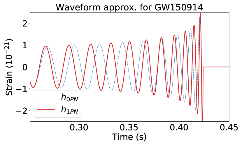
(a) Waveform including (red) and excluding (blue) first order corrections. The waveform was plotted for values matching those of Table 1 of [1]. The plot depicts the waveform as seen in the detector frame, i.e. cosmologically redshifted.

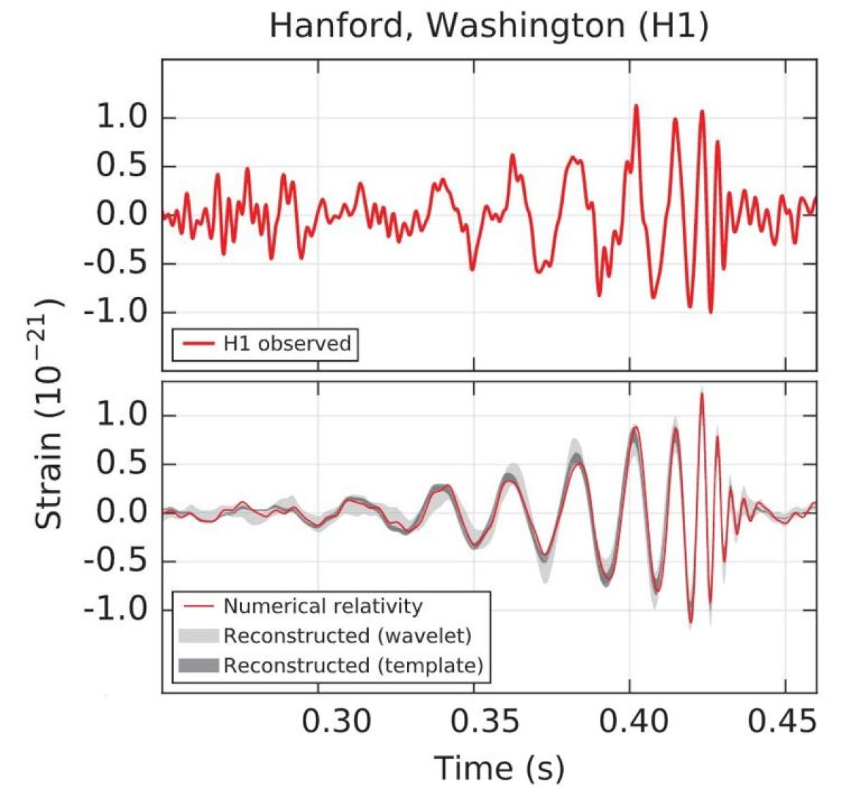
(b) Data and model by LIGO for GW150914, published in [1].

Figure 2.1: Waveform based on computations of this thesis (2.1(a)) and LIGO’s data and model (2.1(b)) for comparison. The plots share a similar structure, but it is clear by figure (2.1(b)) that the signal-to-noise ratio is small, and much of the early-time structure is ‘washed out’ by noise. That is to say, both the signal and the model in (2.1(b)) has been filtered by frequency, making the plots somewhat jagged. Plot (2.1(a)) has not been filtered. In figure (2.1(a)) the amplitude diverges at $t=0.425$s, while in the in (2.1(b)) it does not. This is because the inspiral model breaks down here, and the merger phase takes over.

All that remains now to obtain the waveform is to find the amplitude of the different harmonics, and multiply them by $\cos(n\Phi(\tau))$. By using expression (LABEL:eq:H:rad:fromMultipoles) from LABEL:chap:flux the amplitude of the $h_{1\text{\lx@glossaries@gls@link{acronym}{pn}{\leavevmode PN}}}$ can be found to be

$$\begin{split}h_{1\text{\lx@glossaries@gls@link{acronym}{pn}{\leavevmode PN}}}(\tau)=-\frac{4G(1+z)\mu}{Rc^{2}}v^{2}_{\text{1\lx@glossaries@gls@link{acronym}{pn}{\leavevmode PN}}}(\tau)\Biggl{\{}&\left(1-\frac{23+27\eta}{42}\frac{v^{2}_{\text{0\lx@glossaries@gls@link{acronym}{pn}{\leavevmode PN}}}(\tau)}{c^{2}}\right)\cos\left(2\Phi(\tau)\right)\\ &+\frac{77\sqrt{1-4\eta}}{60}\frac{v_{\text{0\lx@glossaries@gls@link{acronym}{pn}{\leavevmode PN}}}(\tau)}{c}\sin\left(2\Phi(\tau)\right)\Biggr{\}}.\end{split}$$ (2.20)

Here $z$ is the cosmological redshift, see [16] for a derivation. This function is plotted in Figure 2.1(a) using numbers from table 1 of [1] for $R$, $z$, $m_{1}$, and $m_{2}$. The functions $v(\tau)$ and $\Phi(\tau)$ are given by equation (2.17) and (2.19) respectively. The 0PN amplitude is obtained by using $v_{\text{0\lx@glossaries@gls@link{acronym}{pn}{\leavevmode PN}}}(\tau)$ and neglecting the correctional terms inside the curly bracket that contain a factor of $c^{-1}$.

In Figure 2.1(a) it is clear that 1PN corrections does not affect the amplitude much directly, but it has significant effect on the time evolution of the phase, and hence the frequency spectrum. It is however noticeable that the phase of Figure 2.1(a) does not match up with Figure 2.1(b). Either higher order corrections are required, or the model breaks down for such low values of $\tau$.

2.2.2 Computing the Fourier transform of the waveform

To obtain the high sensitivities in GW detections the signal is Fourier transformed, in order to show which frequencies dominate the signal. This frequency spectrum can be compared to theoretical predictions to determine factors like the total mass at 0PN, symmetric mass ratio at 1PN, and more parameters at higher orders, e.g. spin at 1.5PN [12] and finite size effects like tidal deformation at 5PN [17].

In order to compare data with theoretical predictions these predictions must also be expressed in the frequency domain. Therefore, the desired waveform is $\Psi(f)$, which is the phase of the Fourier transformed waveform.

The Fourier transform and stationary phase approximation

To compute the Fourier transformed $\tilde{B}(f)$ of some function $B(t)$ the stationary phase approximation (SPA)can be used, and it is commonly utilized to compute the Fourier transform of (2.3). Standardized in GW physics by [18] it approximates

$$\mbox{for\quad}B(t) =A(t)\cos(\Phi(t)),$$

$$\begin{split}\Rightarrow\quad\tilde{B}(f)&\approx\frac{1}{2}A(t)\left(\derivative{f}{t}\right)^{-1/2}\exp{i\left(2\pi ft-\Phi(f)-\pi/4\right)}\\ &\equiv\frac{1}{2}A(t)\left(\derivative{f}{t}\right)^{-1/2}\exp{i\Psi(f)},\end{split}$$ (2.21)

provided $$\derivative{\ln{A(t)}}{t}\ll\derivative{\Phi}{t}\mbox{\quad and\quad}\derivative[2]{\Phi}{t}\ll\left(\derivative{\Phi}{t}\right)^{2}.$$

This is exactly the type of expression which describes GW s (2.3), and the conditions do indeed apply to the inspiral phase.

The leading order amplitude scales as $v^{2}\sim\tau^{-1/4}$ (2.17) (also, see equation (LABEL:eq:Linearized:GWfromNewtonBinary:FinalExpression) in the next chapter for why the amplitude scales as $v^{2}$), while $\differential\Phi/\differential t=\omega(\tau)\sim\tau^{-3/8}$ (see (2.18)). Thus, for large $\tau$, which is the time remaining till coalescence, $\differential{\ln{a_{n}(t)}}/\differential t\sim\frac{1}{4}\tau^{-1}\ll\omega(\tau)\sim\tau^{-3/8}$.

As for the last prerequisite it can be shown to hold for quasi-stable circular orbit s. Taking the time derivative of Kepler’s third law (2.4) results in

$$2\omega\dot{\omega} =-3\dot{r}\frac{GM}{r^{4}}=-3\frac{\dot{r}}{r}\omega^{2},$$

$$\Rightarrow\quad \frac{-\dot{r}}{\omega r}=\frac{2}{3}\frac{\dot{\omega}}{\omega^{2}}\ll 1.$$ (2.22)

For quasi-stable circular orbit s the inspiral must be slow compared to the orbital motion, and thus the radial velocity ($\dot{r}$) must be small compared to the tangential velocity ($\omega r$), since for perfectly circular motion their fraction is identically zero. From Kepler’s law this implies also that $\dot{\omega}/\omega^{2}\ll 1\to\ddot{\Phi}\ll\dot{\Phi}^{2}$, which is exactly the condition required to use the SPA.

This in hand also provides an estimate for the validity of this approximation, as $\omega$ is a known function of time (2.18)

$$\frac{2}{3}\frac{\dot{\omega}}{\omega^{2}}\stackrel{{\scriptstyle\eqref{eq:waveform:omegaOfTau}}}{{\simeq}}\frac{2}{5}\left(\frac{5G\M}{c^{3}}\right)^{5/8}\tau^{-5/8}\ll 1.$$ (2.23)

This expression is indeed small for most values of $t<t_{c}$.

Since the most important part of the waveform for comparisons to experimental data is the frequency spectrum, the last computation of this chapter will be of the Fourier transformed phase $\Psi(f)$.

Computing the SPA waveform

From equation (2.21) the phase of the Fourier transformed waveform can be approximated as

$$\Psi\ind{{}_{\text{\lx@glossaries@gls@link{acronym}{spa}{\leavevmode SPA}}}}=2\pi ft(f)-\Phi(f)=\omega t(\omega)-\Phi(\omega)=\frac{v^{3}}{GM}t(v)-\Phi(v).$$ (2.24)

$\Phi(v)$ being given by equation (2.14), and $t(v)$ by (2.16), $\Psi(v)$ can easily be computed.

$$\frac{v^{3}}{GM}t(v) =\frac{v^{3}}{GM}t_{c}-\frac{5}{2^{8}}\frac{1}{\eta}\frac{c^{5}}{v^{5}}\left\{1+\frac{8}{6}\left(\frac{743}{336}+\frac{11}{4}\eta\right)\frac{v^{2}}{c^{2}}+\dots\right\},$$ (2.25)

$$\Psi\ind{{}_{\text{\lx@glossaries@gls@link{acronym}{spa}{\leavevmode SPA}}}}(v)=\frac{v^{3}}{GM}t_{c}-\Phi_{0}+\frac{3}{256}\frac{1}{\eta}\frac{c^{5}}{v^{5}}\left\{1+\left(\frac{3715}{756}+\frac{55}{9}\eta\right)\frac{v^{2}}{c^{2}}+\dots\right\}.$$ (2.26)

Lastly the phase can be expressed in terms of the physical frequency by using $v=(GM\omega)^{1/3}=(2\pi GMf)^{1/3}$.

$$\begin{split}\Psi\ind{{}_{\text{\lx@glossaries@gls@link{acronym}{spa}{\leavevmode SPA}}}}(f)=\hskip 3.0pt&2\pi ft_{c}-\Phi_{0}+\frac{3}{256}\left(\frac{2\pi G\M f}{c^{3}}\right)^{-\frac{5}{3}}\\ &\cdot\left\{1+\left(\frac{3715}{756}+\frac{55}{9}\eta\right)\left(\frac{2\pi GMf}{c^{3}}\right)^{\frac{2}{3}}\right\}.\end{split}$$ (2.27)

This is indeed equivalent to the expression found by [12] (equation (6.22), page 21) up to 1PN, with some difference in notation.

In order to compute this waveform all that is needed is the PN expansion of the orbital energy, and the GW energy flux, both associated with stable, energy conservative, motion. In [12] these were provided with references to other papers.

In a sense, (2.27) is the final result of this thesis, computation wise, but it now remains to justify the expressions used for the post-Newtonian expansion of the orbital energy (2.7), and energy flux expansion (2.8), which will be derived in LABEL:chap:energy and LABEL:chap:flux respectively.

Chapter 3 Gravity as a gauge theory

In this chapter the fundamental theory by which the orbital energy and energy flux will be calculated is derived. How can Einstein’s general relativity be described as a classical field theory, and then recast into the language of EFT.

The derivations presented in this chapter largely follows those presented in [19], with supplements from [16] and [11].

3.1 Background

The modern theory of gravity is partially split between two traditions. On the one hand there is the geometrical tradition following Einstein’s approach by interpreting gravity as the effect of a curved space-time, which is curved according to the Einstein’s field equations. The followers of this tradition may be called relativists. On the other hand there is the tradition of using the formalism of Lorentz invariant fields on a static, Minkowskian, space-time, inspired by its monumental success for electrodynamics and quantum theory. The followers of this tradition may be called field theorists.

Though these traditions are not entirely separated, the two different interpretations lend themselves to different natural extensions of general relativity. Thus the two traditions tend to separate relativists and field theorists by which theories they work on.

In this thesis the 1PN phase of GW produced by compact binaries are computed using the formalism of field theory. Familiarity with basic quantum field theory (QFT)is expected, but the derivations are otherwise supposed to be elementary.

Feynman and gravity

One of the most famous field theorists, R. P. Feynman had a “gravity phase” from 1954 to the late 1960s ([20]). After having worked on the foundations of quantum electrodynamics, Feynman sought to uncover the quantum nature of gravity pursuing a similar method. He reckoned that gravity could, similarly to electromagnetism, be perturbatively expanded with respect to its coupling constant, and then quantized by quantizing the frequencies.

Quantizing gravity turns out to be a little more complicated than that, but Feynman’s approach to classical gravity as a massless, spin 2, gauge field has made a lasting impression on gravity physics, especially in the context of GW s. This approach can be studied in the lecture notes from his lecture series of the 60’s [19].

3.2 Fierz-Pauli Lagrangian

To linearized order of the field ($h\ind{{}_{\mu\nu}}$) in the resulting EoM, the Einstein-Hilbert action of general relativity is equivalent to the massless Fierz-Pauli action from field theory [21].

3.2.1 Deriving the graviton Lagrangian

When Feynman set out to study gravity, he took the mindset of a field theorist who until recently was unaware of gravitation, and just now have been presented with data suggesting that all masses attract other masses according to an inverse square law, proportional to the product of their masses,

$$\tvec{F}\sim-\frac{m_{1}m_{2}\tvec{r}}{r^{3}}.$$

Feynman envisioned this as the mindset of aliens on Venus who had just now acquired the technology to pierce through the atmosphere and measure the movement of the planets, but were still our equals in particle physics.

Their first impulse would probably be to guess that this is an unknown effect of some known field. After finding no field that could replicate the solar system observation, their next guess would be that there exists a new kind of field which mediates this mysterious force. Calling this hypothetical field the graviton field, and its associated quantum particle the graviton, the Venusians would next try to uncover its structure.

To construct the Lagrangian for this new force of nature they would determine that it has to be of even spin, and thus an even tensor rank, for the resulting static force to be attractive for equal charges, where the charge for the graviton field would be mass. For the force to go as an inverse square the field must also be massless.

Lastly, it must couple to all matter equally, but it must do so in a relativistic way. The natural suggestion is to somehow couple the field with the four-velocity of the source, like how the electric charge which the electric field couples to is promoted to the charge density four current $j^{\mu}=\gamma^{-1}\rho u^{\mu}$, and couples to the vector potential $A_{\mu}=\MixVec{\phi/c}{A_{i}}$. See [22] or other textbooks on relativistic field theory.

However, to let the graviton field couple to all fields a natural candidate is the energy-momentum tensor $T\ind{{}^{\mu\nu}}$, induced by field invariance under space-time translations. Incidentally, for a point particle it is constructed by the four-velocity of the source: $T\ind{{}^{\mu\nu}}=\gamma^{-1}p\ind{{}^{\mu}}u\ind{{}^{\nu}}=\gamma^{-1}\rho u\ind{{}^{\mu}}u\ind{{}^{\nu}}$. Now for a scalar field it can be contracted to form a scalar, the trace, which is proportional to the mass density. Alternatively, a field of higher tensor rank can couple to the indices, also coupling the field to the mass density in the static frame $T\ind{{}^{\mu\nu}}=T\ind{{}^{00}}\delta\ind{{}^{\mu 0}}\delta\ind{{}^{\nu 0}}$.

The spin zero / scalar field is a candidate for the graviton, but fails to couple to the electromagnetic energy-momentum tensor, as the electromagnetic energy-momentum tensor is traceless. It also fails to predict the perihelion procession of Mercury correctly [22].

Thus, the Venusians would probably try a massless spin 2 field next. Since massless fields only have one (spin $s=0$) or two degrees of freedom (helicity $=\pm s$) the symmetric spin two field should be easiest to work with, as it will have $10-2=8$ redundant degrees of freedom. The antisymmetric field by comparison only have $6-2=4$ redundant degrees of freedom.

Thus demanding the Lagrangian to be composed of a massless, symmetric, rank two tensor field there are only four unique terms, containing only second / two derivatives, after considering partial integrations:

1. Two where the index of the tensor and the index of the derivative differ.

2. $h\ind{{}_{\mu\nu,\rho}}h\ind{{}^{\mu\nu,\rho}}$

3. $h\ind{{}_{\mu\nu,\rho}}h\ind{{}^{\mu\rho,\nu}}$

4. And three where two of the indices contract for the individual $h\ind{{}_{\mu\nu}}$.

5. $h\ind{{}_{\mu\nu}^{,\nu}}h\ind{{}^{\mu\rho}_{,\rho}}$

6. $h\ind{{}_{\mu\nu}^{,\nu}}h\ind{{}^{,\mu}}\mbox{\quad with\quad}h\equiv h\ind{{}_{\sigma}^{\sigma}}$

7. $h\ind{{}_{,\mu}}h\ind{{}^{,\mu}}$

Why are these terms of quadratic order in $h\ind{{}_{\mu\nu}}$? Because it is action terms of quadratic order in a field which yields EoM s of linear order of that field.

Note that term number 2. and 3. are the same after two successive partial integrations $h\ind{{}_{\mu\nu,\rho}}h\ind{{}^{\mu\rho,\nu}}=-h\ind{{}_{\mu\nu}}h\ind{{}^{\mu\rho,\nu}_{\rho}}=h\ind{{}_{\mu\nu}^{,\nu}}h\ind{{}^{\mu\rho}_{,\rho}}$. Some texts use term 2. (like [16]), but here term 3. will be employed (like in [19]). Thus, the free part of the Lagrangian must be of the form

$$\L=a_{1}h\ind{{}_{\mu\nu,\rho}}h\ind{{}^{\mu\nu,\rho}}+a_{2}h\ind{{}_{\mu\nu}^{,\nu}}h\ind{{}^{\mu\rho}_{,\rho}}+a_{3}h\ind{{}_{\mu\nu}^{,\nu}}h\ind{{}^{,\mu}}+a_{4}h\ind{{}_{,\mu}}h\ind{{}^{,\mu}}.$$ (3.1)

It is possible to determine all the coefficients $a_{1-4}$ by imposing gauge invariance on the equation of motion (EoM). The EoM for fields is determined by the Euler-Lagrange equation (3.2a) (see e.g. [2], or [24]), and for (3.1) the equation of motion becomes (3.2c).

$$\partial_{\rho}\partialderivative{\L}{h\ind{{}_{\mu\nu,\rho}}}- \partialderivative{\L}{h\ind{{}_{\mu\nu}}}=0$$ (3.2a)

$$=\partial\ind{{}_{\rho}}\Bigl{(}2a_{1}h\ind{{}^{\mu\nu,\rho}}+a_{2}\eta\ind{{}^{\nu\rho}}h\ind{{}^{\mu\sigma}_{,\sigma}}+a_{2}\eta\ind{{}^{\mu\rho}}h\ind{{}^{\nu\sigma}_{,\sigma}}+a_{3} \eta\ind{{}^{\nu\rho}}h\ind{{}^{,\mu}}+a_{3}\eta\ind{{}^{\mu\nu}}h\ind{{}^{\rho\sigma}_{,\sigma}}+2a_{4}\eta\ind{{}^{\mu\nu}}h\ind{{}^{,\rho}}\Bigr{)}$$ (3.2b)

$$=2a_{1}h\ind{{}^{\mu\nu,\rho}_{\rho}}+a_{2}h\ind{{}^{\mu\rho,\nu}_{\rho}}+a_{2}h\ind{{}^{\nu\rho,\mu}_{\rho}}+a_{3}h\ind{{}^{,\mu\nu}}+ a_{3}\eta\ind{{}^{\mu\nu}}h\ind{{}^{\rho\sigma}_{,\rho\sigma}}+2a_{4}\eta\ind{{}^{\mu\nu}}h\ind{{}^{,\rho}_{\rho}}\equiv\Xi\ind{{}^{\mu\nu}}.$$ (3.2c)

From the action of $\L+\L_{\text{int}}=\L+\frac{\lambda}{2}h\ind{{}_{\mu\nu}}T\ind{{}^{\mu\nu}}$ the inferred EoM should be

$$\Xi\ind{{}^{\mu\nu}} =-\frac{1}{2}\lambda T\ind{{}^{\mu\nu}},$$ (3.3a)

$$T\ind{{}^{\mu\nu}_{,\nu}}=0\quad \Rightarrow\quad\Xi\ind{{}^{\mu\nu}_{,\nu}}=0.$$ (3.3b)

Equation (3.3b) can be used to fix the coefficients of equation (3.2c), and thus also the Lagrangian.

$$\Xi\ind{{}^{\mu\nu}_{,\nu}}=\dalembertian h\ind{{}^{\mu\nu}_{,\nu}}(2a_{1}+a_{2})+\dalembertian h\ind{{}^{,\mu}}( a_{3}+2a_{4})+h\ind{{}^{\rho\sigma,\mu}_{\rho\sigma}}(a_{2}+a_{3})=0,$$

$$\Rightarrow\quad a_{1}=-\frac{1}{2}a_{2} =\frac{1}{2}a_{3}=-a_{4}.$$ (3.4)

Thus a Lagrangian of a symmetric, massless, rank 2 tensor field which couples to a divergenceless rank 2 tensor field (e.g. $\L_{\text{int}}=-\frac{\lambda}{2}h\ind{{}_{\mu\nu}}T\ind{{}^{\mu\nu}}$), consisting of only second derivatives, in a flat space-time, must to second power of $h$ take the form of the massless Fierz-Pauli Lagrangian [21]

$$\L_{\text{\lx@glossaries@gls@link{acronym}{fp}{\leavevmode FP}}}=-\frac{1}{2}h\ind{{}_{\mu\nu,\rho}}h\ind{{}^{\mu\nu,\rho}}+h\ind{{}_{\mu\nu}^{,\nu}}h\ind{{}^{\mu\rho}_{,\rho}}-h\ind{{}_{\mu\nu}^{,\nu}}h\ind{{}^{,\mu}}+\frac{1}{2}h\ind{{}_{,\mu}}h\ind{{}^{,\mu}}.$$ (3.5)

Here the overall factor has been set to $a_{1}=-1/2$.

3.2.2 The equation of motion and gauge condition

The EoM for $\L_{\text{\lx@glossaries@gls@link{acronym}{fp}{\leavevmode FP}}}+\frac{1}{2}\lambda h\ind{{}_{\mu\nu}}T\ind{{}^{\mu\nu}}$ follows directly from the Euler-Lagrange equation (3.2a) as

$$-\dalembertian h\ind{{}_{\mu\nu}}+2h\ind{{}^{\alpha}_{\{\mu,\nu\}\alpha}}-h\ind{{}_{,\mu\nu}}-\eta\ind{{}_{\mu\nu}}\left(h\ind{{}_{\rho\sigma}^{,\rho\sigma}}-\dalembertian h\right)=\frac{\lambda}{2}T\ind{{}_{\mu\nu}}.$$ (3.6)

This is equivalent with the equation of motion found in the linear approximation of general relativity, for an appropriate choice of $\lambda$ (see e.g. equation (1.17) of [16], or equation (9.16) of [25])

Varying the Fierz-Pauli action directly should also provide the equations of motion

$$\variation{\L_{\text{\lx@glossaries@gls@link{acronym}{fp}{\leavevmode FP}}}}=\hskip 3.0pt \functionalderivative{\L_{\text{\lx@glossaries@gls@link{acronym}{fp}{\leavevmode FP}}}}{h\ind{{}_{\mu\nu,\rho}}}\variation{h\ind{{}_{\mu\nu,\rho}}}+\functionalderivative{\L_{\text{\lx@glossaries@gls@link{acronym}{fp}{\leavevmode FP}}}}{h\ind{{}_{\mu\nu}}}\variation{h\ind{{}_{\mu\nu}}}=\functionalderivative{\L_{\text{\lx@glossaries@gls@link{acronym}{fp}{\leavevmode FP}}}}{h\ind{{}_{\mu\nu,\rho}}}\partial\ind{{}_{\rho}}\variation{h\ind{{}_{\mu\nu}}}+\functionalderivative{\L_{\text{\lx@glossaries@gls@link{acronym}{fp}{\leavevmode FP}}}}{h\ind{{}_{\mu\nu}}}\variation{h\ind{{}_{\mu\nu}}}$$

$$= \left[\functionalderivative{\L_{\text{\lx@glossaries@gls@link{acronym}{fp}{\leavevmode FP}}}}{h\ind{{}_{\mu\nu}}}-\partial\ind{{}_{\rho}}\functionalderivative{\L_{\text{\lx@glossaries@gls@link{acronym}{fp}{\leavevmode FP}}}}{h\ind{{}_{\mu\nu,\rho}}}\right]\variation{h\ind{{}_{\mu\nu}}}=-\Xi\ind{{}^{\mu\nu}}\variation{h\ind{{}_{\mu\nu}}}=0.$$ (3.7)

This automatically holds because of (3.2c) ($\Xi\ind{{}^{\mu\nu}}=0$). But (3.7) can also be solved using the condition (3.3b), $\Xi\ind{{}^{\mu\nu}_{,\nu}}=0$. Letting $\variation{h\ind{{}_{\mu\nu}}}=-\xi\ind{{}_{\mu,\nu}}-\xi\ind{{}_{\nu,\mu}}$ it is easy to show that the action stays invariant under this type of transformation, using partial integration.

$$\variation{\L_{\text{\lx@glossaries@gls@link{acronym}{fp}{\leavevmode FP}}}}=\Xi\ind{{}^{\mu\nu}}\left(\xi\ind{{}_{\mu,\nu}}+\xi\ind{{}_{\nu,\mu}}\right)=-\Xi\ind{{}^{\mu\nu}_{,\nu}}\xi\ind{{}_{\mu}}-\Xi\ind{{}^{\mu\nu}_{,\mu}}\xi\ind{{}_{\nu}}=-2\Xi\ind{{}^{\mu\nu}_{,\nu}}\xi\ind{{}_{\mu}}\stackrel{{\scriptstyle\eqref{eq:EoMLh2MustBeDivergenceless}}}{{=}}0.$$ (3.8)

Thus the following transformation of the field leaves both the EoM and the gauge condition invariant.

$$h\ind{{}_{\mu\nu}}(x)\to h\ind{{}_{\mu\nu}}(x)+\variation{h\ind{{}_{\mu\nu}}(x)}=h\ind{{}_{\mu\nu}}(x)-\xi\ind{{}_{\mu,\nu}}(x)-\xi\ind{{}_{\nu,\mu}}(x).$$ (3.9)

Again, this is equivalent to the gauge condition found in linear theory when linearizing metric invariance under change of coordinates (see equation (9.9) of [25]).

Also introducing the commonly used bar operator, which symmetrize tensors and changes the sign of their trace,

$$\bar{S}\ind{{}_{\mu\nu}}\equiv\frac{1}{2}\left(S\ind{{}_{\mu\nu}}+S\ind{{}_{\nu\mu}}-S\ind{{}^{\sigma}_{\sigma}}\eta\ind{{}_{\mu\nu}}\right),$$ (3.10)

the gauge condition for the barred $h$-field is obtained by transforming (3.9) as (3.10), resulting with

$$\bar{h}\ind{{}_{\mu\nu}}(x)\to\bar{h}\ind{{}_{\mu\nu}}(x)-\xi\ind{{}_{\mu,\nu}}(x)-\xi\ind{{}_{\nu,\mu}}(x)+\eta\ind{{}_{\mu\nu}}\xi\ind{{}_{\sigma}^{,\sigma}}(x)\equiv\bar{h}\ind{{}_{\mu\nu}}(x)-\xi\ind{{}_{\mu\nu}}(x).$$ (3.11)

Thus the divergence of this barred field transforms as

$$\bar{h}\ind{{}_{\mu\nu}^{,\nu}}\to\bar{h}\ind{{}_{\mu\nu}^{,\nu}}-\dalembertian\xi\ind{{}_{\mu}}.$$ (3.12)

As $\xi_{\mu}$ can be any vector without changing the EoM, it can be chosen such that $\dalembertian\xi\ind{{}_{\mu}}=\bar{h}\ind{{}_{\mu\nu}^{,\nu}}$, shifting the field such that $\bar{h^{\prime}}\ind{{}_{\mu\nu}^{,\nu}}=0$, which is to impose the Lorenz gauge.

Lorenz $$\text{gauge condition}:$$

$$\bar{h}\ind{{}_{\mu\nu}^{,\nu}}=0.$$ (3.13)

The exact expression for $\xi_{\mu}$ can be obtained by method of Green’s functions, but this is unnecessary to compute. Simply keeping in mind that $\bar{h^{\prime}}\ind{{}_{\mu\nu}^{,\nu}}=0$ shall suffice to simplify the Lagrangian (3.5). Notice that the following terms must be zero, using again (3.10), but in reverse.

$$\bar{h}\ind{{}_{\mu\nu}^{,\nu}}=\hskip 3.0pt 0=h\ind{{}_{\mu\nu}^{,\nu}}-\frac{1}{2}\eta\ind{{}_{\mu\nu}}h\ind{{}^{,\nu}},$$ (3.14a)

$$\bar{h}\ind{{}_{\mu\nu}^{,\nu}}\bar{h}\ind{{}^{\mu\rho}_{,\rho}}=\hskip 3.0pt 0^{2}=h\ind{{}_{\mu\nu}^{,\nu}}h\ind{{}^{\mu\rho}_{,\rho}}-h\ind{{}_{\mu\nu}^{,\nu}}h\ind{{}^{,\mu}}+\frac{1}{4}h\ind{{}_{,\mu}}h\ind{{}^{,\mu}}.$$ (3.14b)

Adding and subtracting 0 from the Lagrangian should change nothing, and thus the following expression can be used as a gauge fixing term (gf)

$$\L_{\text{\lx@glossaries@gls@link{acronym}{gf}{\leavevmode gf}}}=-\bar{h}\ind{{}_{\mu\nu}^{,\nu}}\bar{h}\ind{{}^{\mu\rho}_{,\rho}}=\left[-h\ind{{}_{\mu\nu}^{,\nu}}h\ind{{}^{\mu\rho}_{,\rho}}+h\ind{{}_{\mu\nu}^{,\nu}}h\ind{{}^{,\mu}}-\frac{1}{4}h\ind{{}_{,\mu}}h\ind{{}^{,\mu}}\right],$$ (3.15)

$$\Rightarrow\quad\L_{(2)}+ \L_{\text{int}}\equiv\L_{\text{\lx@glossaries@gls@link{acronym}{fp}{\leavevmode FP}}}+\L_{\text{\lx@glossaries@gls@link{acronym}{gf}{\leavevmode gf}}}+\L_{\text{int}}=-\frac{1}{2}h\ind{{}_{\mu\nu,\rho}}h\ind{{}^{\mu\nu,\rho}}+\frac{1}{4}h\ind{{}_{,\mu}}h\ind{{}^{,\mu}}+\frac{\lambda}{2}h\ind{{}_{\mu\nu}}T\ind{{}^{\mu\nu}}.\quad$$ (3.16)

with the subscript $(2)$ to signify that this is the action to quadratic order in $h$.

The EoM of $\L_{(2)}+\L_{\text{int}}$ is the familiar

$$\dalembertian\left(h\ind{{}_{\mu\nu}}-\frac{1}{2}\eta\ind{{}_{\mu\nu}}h\right)=\dalembertian\bar{h}\ind{{}_{\mu\nu}}=-\frac{\lambda}{2}T\ind{{}_{\mu\nu}},$$ (3.17)

from linearized theory (see equation (1.24) of [16] or equation (9.22) of [25]).

Comparing with the EoM of linearized GR it is tempting to conclude that $\lambda\equiv 4\kappa=32\pi G/c^{4}$, but then it is also common to make the Einstein-Hilbert action dimensionless by scaling it with a factor of $(16\pi G/c^{4})^{-1}$. Comparing (3.16) with the Einstein-Hilbert action expanded to second order the Lagrangian (3.16) carries an additional factor of $2$, and is dimensionful. Field theorists usually fix the dimensionality of the action by rescaling their fields to become dimensionful. Doing this

$$h_{\mu\nu}^{\text{dim.ful}}=\left(\frac{32\pi G}{c^{4}}\right)^{-1/2}h_{\mu\nu}^{\text{dim.less}},$$ (3.18)

$h$ adsorbs the dimensionful prefactor. To compare (3.17) with the linearized Einstein’s field equations, it must first be rescaled back to a dimensionless field according to (3.18), and then the coupling constant is revealed to be

$$\lambda\equiv\left(\frac{32\pi G}{c^{4}}\right)^{1/2}=\sqrt{4\kappa},$$ (3.19)

where $\kappa=\frac{8\pi G}{c^{4}}$ is the constant which appears in Einstein’s field equations.

Some call this coupling constant $M_{\text{Pl}}^{-1}$ rather than $\lambda$ ([11, 3, 26]). However it does not have dimesion of mass, nor is the Planck constant anywhere in the expression, so why do they do this? These articles use natural units $\hbar=c=1$, and $M_{\text{Pl}}^{-1}=\sqrt{G/\hbar c}=\lambda\cdot\sqrt{\hbar c^{3}/32\pi}$, which is just a numerical factor off from $\lambda$ (in natural units).

Furthermore, in natural units, legths $(L)$ are dimesionally equal to inverse mass $(M)^{-1}$ (using $[x]$ as dimesion of $x$: $L=[x]=[ct]=1\cdot T$, and $E=[\hbar\omega]=1\cdot T^{-1}\stackrel{{\scriptstyle\text{also}}}{{=}}[mc^{2}]=M\cdot 1^{2},\quad\Rightarrow\quad M=T^{-1}=L^{-1}=E$), and thus the action has dimension of $[S]=[\int\differential[4]{x}\L]=L^{4}[\L]=M^{-4}[\L]=1$. The action must be dimesionless in QFT, since in the path integral approach it is exponated. Every field Lagrangian has a kinetic term $\sim\partial\phi\partial\phi$, which scale as $[\L]=M^{4}=[\partial\phi]^{2}=L^{-2}[\phi]^{2}=M^{2}[\phi]^{2}\quad\Rightarrow\quad[\phi]=M$. Thus for couplings $\L_{\text{int}}\sim\lambda h(\partial h)^{2}$ to have the same dimension as the kinetic term; $[\lambda]=M^{-1}$.

Calling the coupling constant $M_{\text{Pl}}^{-1}$ might have the unfortunate consequense of making it look like a quantum theory, but make no mistake, this is all classical field theory. Therefore, it is simply labelled $\lambda$ in this thesis.

3.3 Solutions of the graviton field

3.3.1 Gravitational waves in vacuum, and their polarization

According to the equation of motion (3.17) the field will in a vacuum ($T\ind{{}_{\mu\nu}}=0$) behave as a relativistic wave

$$\dalembertian\bar{h}\ind{{}_{\mu\nu}}=0,$$ (3.20)

which admits solutions of the form (2.2). See Appendix A for a derivation of this solution.

Up until now the gauge has only been used to make sure the entire EoM (3.17) remains divergence free, just like the source term $T\ind{{}_{\mu\nu}^{,\nu}}=0$. In doing so it was determined that the field might only be shifted according to (3.9). Furthermore, the divergence of the barred $h$-field could be eliminated only imposing further that $\dalembertian\xi_{\mu}=0$.

Keeping $\dalembertian\xi_{\mu}=0$ still leaves

$$\xi\ind{{}_{\mu\nu}}(x)\equiv\xi\ind{{}_{\mu,\nu}}(x)+\xi\ind{{}_{\nu,\mu}}(x)-\eta\ind{{}_{\mu\nu}}\xi\ind{{}_{\sigma}^{,\sigma}}(x)$$ (3.21)

with four degrees of freedom, as it is a function of the four independent parameters $\xi_{\mu}$, which satisfy $\dalembertian\xi_{\mu}=0$. To make the graviton field divergence free imposes four additional conditions on $h\ind{{}_{\mu\nu}}$, by the four equations $h\ind{{}_{\mu\sigma}^{,\sigma}}=0$. This leaves $h\ind{{}_{\mu\nu}}$ with $10-4=6$ degrees of freedom. Subtracting further the four gauge freedoms reduces $h\ind{{}_{\mu\nu}}$ to only two effective degrees of freedom, as any massless spin two field should have. These four gauge freedoms $\xi_{\mu}$ can be used to impose four additional conditions on $\bar{h}\ind{{}_{\mu\nu}}$. $\xi_{0}$ can be used to set the trace $\bar{h}=0$, and since $\bar{h}\ind{{}_{\mu\nu}}$ is just $h\ind{{}_{\mu\nu}}$ with the reversed sign trace, in this gauge $h\ind{{}_{\mu\nu}}=\bar{h}\ind{{}_{\mu\nu}}$.

The three remaining freedoms, $\xi_{i}$, can be used to set $h\ind{{}_{0i}}=0$ as well. Since $h\ind{{}_{\mu\nu}^{,\nu}}=0$ this implies $h\ind{{}_{0\nu}^{,\nu}}=\partial^{0}h\ind{{}_{00}}+\partial^{i}h\ind{{}_{0i}}=0=\partial^{0}h\ind{{}_{00}}$, making $h\ind{{}_{00}}$ a constant of time. A constant contribution to a GW are uninteresting and for all intents and purposes it can be considered to be zero, making all $h\ind{{}_{0\mu}}=0$.

This specific gauge is referred to as the transverse-traceless (TT)gauge, and is defined by

TT gauge condition:

$$h\ind{{}_{0\mu}}=h\ind{{}_{i}^{i}}=h\ind{{}_{ij}^{,j}}=0.$$ (3.22)

Note that this gauge can only be imposed in a vacuum, since the vacuum condition $\dalembertian\bar{h}\ind{{}_{\mu\nu}}=0$ $\Rightarrow$ $\dalembertian\xi\ind{{}_{\mu\nu}}=0$ was used.

Assuming $h\ind{{}_{\mu\nu}}(x^{\alpha})=\epsilon\ind{{}_{\mu\nu}}h(x^{\alpha})$ with $h(x^{\alpha})$ as the scalar solution to the wave equation

$$h(x^{\alpha})=\int\frac{\differential[3]{k}}{(2\pi)^{3}\cdot 2\omega_{k}} \left\{a(\tvec{k})e^{-ik\ind{{}_{\sigma}}x\ind{{}^{\sigma}}}+a^{\dagger}(\tvec{k})e^{ik\ind{{}_{\sigma}}x\ind{{}^{\sigma}}}\right\},$$ (3.23)

which is (A.6) from Appendix A. The TT gauge condition then implies

$$h\ind{{}_{mn}^{,n}}(x^{\alpha})\stackrel{{\scriptstyle\eqref{eq:TT gauge condition}}}{{=}}\hskip 3.0pt 0=\epsilon\ind{{}_{mn}}\partial^{n}h(x^{\alpha})$$

$$=\int\frac{\differential[3]{k}}{(2\pi)^{3}\cdot 2\omega_{k}}\epsilon\ind{{}_{mn}}ik^{n} \left\{-a(\tvec{k})e^{-ik\ind{{}_{\sigma}}x\ind{{}^{\sigma}}}+a^{\dagger}(\tvec{k})e^{ik\ind{{}_{\sigma}}x\ind{{}^{\sigma}}}\right\},$$

hence

$$k\ind{{}^{j}}\epsilon\ind{{}_{ij}}=0.$$ (3.24)

For a wave travelling in the $z$-direction $k_{\mu}=\begin{pmatrix}k,&0,&0,&k\end{pmatrix}$, making $\epsilon\ind{{}_{\mu 3}}=0$. With (3.22) this is enough to determine the polarization down to the two essential degrees of freedom

$$\epsilon\ind{{}_{\mu\nu}}=\begin{pmatrix}0&0&0&0\\ 0&\epsilon_{+}&\epsilon_{\times}&0\\ 0&\epsilon_{\times}&-\epsilon_{+}&0\\ 0&0&0&0\end{pmatrix}=\begin{pmatrix}\epsilon_{+}&\epsilon_{\times}\\ \epsilon_{\times}&-\epsilon_{+}\\ \end{pmatrix}_{\text{in plane $\perp$ to $\tvec{k}$}}.$$ (3.25)

3.3.2 Source of gravitational waves

The general solution of the equation of motion (3.17) with sources can be obtained by method of Green’s functions.

Green’s functions in general

The Green’s function of a linear differential operator $\L\Op_{x}$ is defined as the function that satisfies

$$\L\Op_{x}\Delta(\fvec{x},\fvec{x^{\prime}})=\dirac{n}{\fvec{x}-\fvec{x^{\prime}}}$$

where $\L\Op_{x}$ only acts on $x$.

The differential equation in question

$$\L\Op_{x}\psi(x)=f(x)$$

admits solutions of the form

$$\psi(x)=\int\differential[n]{x^{\prime}}\Delta(x,x^{\prime})f(x^{\prime}).$$

This solution can easily be demonstrated to recover the original differential equation by using the definition of the Green’s function,

$$\L\Op_{x}\psi(x) =\L\Op_{x}\int\differential[n]{x^{\prime}}\Delta(x,x^{\prime})f(x^{\prime})=\int\differential[n]{x^{\prime}}f(x^{\prime})\L\Op_{x}\Delta(x,x^{\prime})$$

$$\stackrel{{\scriptstyle\eqref{eq:Green's func. def}}}{{=}}\int\differential[n]{x^{\prime}}f(x^{\prime})\dirac{n}{x-x^{\prime}}=f(x),$$

which was the original differential equation.

Green’s function of the d’Alembert operator

In our case $\L\Op_{x}=\dalembertian_{x}$, which is invariant under translation. Thus $\Delta(x,x^{\prime})=\Delta(x-x^{\prime})$. In order to find the corresponding Green’s function $\Delta(x-x^{\prime})$ the easiest way is to go through Fourier space.

$$\dalembertian\ind{{}_{x}}\Delta(x-x^{\prime}) =\dalembertian\ind{{}_{x}}\int\frac{\differential[4]{k}}{(2\pi)^{4}}\tilde{\Delta}(k)e^{ik\ind{{}_{\sigma}}(x\ind{{}^{\sigma}}-{x^{\prime}}\ind{{}^{\sigma}})}=\int\frac{\differential[4]{k}}{(2\pi)^{4}}\tilde{\Delta}(k)\left(i^{2}k\ind{{}_{\mu}}k\ind{{}^{\mu}}\right)e^{ik\ind{{}_{\sigma}}(x\ind{{}^{\sigma}}-{x^{\prime}}\ind{{}^{\sigma}})}$$

$$=\dirac{4}{x-x^{\prime}}=\int\frac{\differential[4]{k}}{(2\pi)^{4}}e^{ik\ind{{}_{\sigma}}(x\ind{{}^{\sigma}}-{x^{\prime}}\ind{{}^{\sigma}})}.$$

Matching the last equality of both lines indicates that the Fourier transform of $\Delta(x-x^{\prime})$ must be

$$\Delta(k)=\frac{-1}{k\ind{{}_{\mu}}k\ind{{}^{\mu}}}.$$ (3.26)

Obtaining the Green’s function in real space is now just a matter of transforming (3.26).

One last remark about Green’s functions is in the context of four dimensional space-time the solution in terms of Green’s functions can be understood as counting up contributions from source terms, all over space, and across all time

$$h(x^{\alpha})=\int\differential[4]{x^{\prime}}\Delta(x^{\alpha}-{x^{\prime}}^{\alpha})T({x^{\prime}}^{\alpha})=\int_{-\infty}^{\infty}\differential{ct^{\prime}}\int\differential[3]{x^{\prime}}\Delta(x^{\alpha}-{x^{\prime}}^{\alpha})T({x^{\prime}}^{\alpha}).$$

Thus $\Delta(x-x^{\prime})$ weighs the importance of source contributions at different points in space and time. For physical solutions only contributions of source configurations from the past contribute to $h(t)$. This is imposed by demanding $t\geq t^{\prime}$.

Back to deriving the real space Green’s function. Performing the transform, and defining $r^{\alpha}=x^{\alpha}-{x^{\prime}}^{\alpha}$

$$\Delta(r^{\alpha}) =\int\frac{\differential[4]{k}}{(2\pi)^{4}}\frac{-1}{k\ind{{}_{\mu}}k\ind{{}^{\mu}}}e^{ik\ind{{}_{\sigma}}r\ind{{}^{\sigma}}}=\int\frac{\differential{k\ind{{}_{0}}}}{2\pi}e^{-ik\ind{{}_{0}}r\ind{{}^{0}}}\int\frac{\differential[3]{k}}{(2\pi)^{3}}\frac{1}{k_{0}^{2}-\tvec{k}^{2}}e^{i\tvec{k\cdot r}}$$

$$=\int\frac{\differential{k\ind{{}_{0}}}}{2\pi}e^{-ik\ind{{}_{0}}r\ind{{}^{0}}}\int_{0}^{\infty}\int_{-1}^{1}\int_{0}^{2\pi}\frac{\absolutevalue{\tvec{k}}^{2}\differential{\absolutevalue{\tvec{k}}}\differential{\cos{\theta}}\differential{\phi}}{(2\pi)^{3}}\frac{1}{k_{0}^{2}-\tvec{k}^{2}}e^{i\absolutevalue{\tvec{k}}\absolutevalue{\tvec{r}}\cos{\theta}}$$

$$=\int\frac{\differential{k\ind{{}_{0}}}}{2\pi}e^{-ik\ind{{}_{0}}r\ind{{}^{0}}}\int_{0}^{\infty}\frac{\differential{\absolutevalue{\tvec{k}}}}{(2\pi)^{2}}\frac{\absolutevalue{\tvec{k}}^{2}}{i\absolutevalue{\tvec{k}}\absolutevalue{\tvec{r}}}\frac{e^{i\absolutevalue{\tvec{k}}\absolutevalue{\tvec{r}}}-e^{-i\absolutevalue{\tvec{k}}\absolutevalue{\tvec{r}}}}{k_{0}^{2}-\tvec{k}^{2}},$$

where the spatial integral was performed in spherical coordinates. Relabelling $\absolutevalue{\tvec{k}}=k$ and $\absolutevalue{\tvec{r}}=r$, the expression can be worked further

$$\Delta(r^{\alpha}) =\int\frac{\differential{k\ind{{}_{0}}}}{2\pi}e^{-ik\ind{{}_{0}}r\ind{{}^{0}}}\int_{-\infty}^{\infty}\differential{k}\frac{k}{i(2\pi)^{2}r}\frac{e^{ikr}}{k_{0}^{2}-k^{2}}.$$

Extending to the complex plane, this integral can be evaluated using Cauchy’s residue theorem, from complex analysis. Shifting $k\ind{{}_{0}}\to k\ind{{}_{0}}+i\varepsilon$ is equivalent to imposing the retardation condition: $t\geq t^{\prime}\Leftrightarrow r\ind{{}^{0}}\geq 0$. Why this is the case should become apparent soon. According to the residue theorem

$$\begin{split}&\oint\differential{z}f(z)=i2\pi\sum_{k}\text{Res}(f,a_{k}),\\ \text{where $a_{k}$ is }&\text{a pole of $f(z)$ enclosed by the integral, and}\\ &\text{Res}(f,a_{k})=\lim_{z\to a_{k}}(z-a_{k})\cdot f(z).\end{split}$$ (3.27)

Utilizing this theorem and integrating over the upper complex plane, the Green’s function becomes

$$\Delta(r^{\alpha}) =\lim_{\varepsilon\to 0}\int\frac{\differential{k\ind{{}_{0}}}}{2\pi}e^{-ik\ind{{}_{0}}r\ind{{}^{0}}}\frac{-1}{i(2\pi)^{2}r}\oint\differential{k}k\frac{e^{ikr}}{(k-k_{0}-i\varepsilon)(k+k_{0}+i\varepsilon)}$$

$$=\lim_{\varepsilon\to 0}\int\frac{\differential{k\ind{{}_{0}}}}{2\pi}e^{-ik\ind{{}_{0}}r\ind{{}^{0}}}\frac{-1}{i(2\pi)^{2}r}\frac{i2\pi}{2}e^{ir(k\ind{{}_{0}}+i\varepsilon)}$$

$$=\frac{-1}{4\pi r}\int\frac{\differential{k\ind{{}_{0}}}}{2\pi}e^{-ik\ind{{}_{0}}(r\ind{{}^{0}}-r)}=\frac{-\dirac{}{ct-r}}{4\pi r}$$

It is now apparent that this is the retarded solution. Had $k_{0}$ rather been shifted by $-i\varepsilon$, the Dirac delta function would have been $\dirac{}{ct+r}$. The delta function picks out contributions on the light cone of $x^{\alpha}$, the retarded Green’s function picks out on the past light cone, while the advanced Green’s function picks out on the future light cone.

$$\Delta_{\text{ret}}(r^{\alpha}) =\frac{-\dirac{}{ct-\absolutevalue{\tvec{r}}}}{4\pi\absolutevalue{\tvec{r}}}.$$ (3.28a)

$$\Delta_{\text{adv}}(r^{\alpha}) =\frac{-\dirac{}{ct+\absolutevalue{\tvec{r}}}}{4\pi\absolutevalue{\tvec{r}}}.$$ (3.28b)

Beyond singling out contributions from the light cone, it is apparent that the importance of each contribution to the field is weighted by how far away it is from the point in question, according to the inverse power of the spatial distance.

Solving the inhomogeneous equation of motion

Back to the EoM (3.17), using the retarded Green’s functions it admits solution of the form

$$\dalembertian\bar{h}\ind{{}_{\mu\nu}}(x) =-\frac{\lambda}{2}T\ind{{}_{\mu\nu}}(x)$$

$$\Rightarrow\quad\bar{h}\ind{{}_{\mu\nu}}(\fvec{x}) =-\frac{\lambda}{2}\int\differential[4]{x^{\prime}}\Delta_{\text{ret}}(\fvec{x}-\fvec{x^{\prime}})T\ind{{}_{\mu\nu}}(\fvec{x^{\prime}})$$

$$=\frac{\lambda}{8\pi}\int\differential[3]{x^{\prime}}\frac{T\ind{{}_{\mu\nu}}(t_{\text{ret}},\tvec{x^{\prime}})}{\absolutevalue{\tvec{x}-\tvec{x^{\prime}}}},\mbox{\quad where $t_{\text{ret}}\equiv t-\frac{\absolutevalue{\tvec{x}-\tvec{x^{\prime}}}}{c}$.\quad}$$ (3.29)

Assuming the GW is measured far away from the source compared to the size of the source system, then the approximation $\absolutevalue{\tvec{x}-\tvec{x^{\prime}}}\approx\absolutevalue{\tvec{x}}\equiv R$ holds. This simplifies the integral in equation (3.29) to only be dependent on the energy distribution of the source, and not where it is measured.

Furthermore, waves measured in vacuum can be set into the TT gauge, which implies that all physical information of the source can be captured by its spatial indices $\bar{h}\ind{{}_{ij}}$.

Using this leading order term of (LABEL:eq:EnergyMultipole:allOrders) and (LABEL:eq:pp_EnergyMomentumTensor) for the $\T^{00}$ term the resulting leading order expression for the mass quadrupole moment is

$$\begin{split}I^{ij}_{(0)}(t)&=\frac{(5)!!}{(5)!!}\int\differential[3]{x}\T\ind{{}^{00}}(t,\tvec{x})\left[x^{i}x^{j}\right]_{\text{\lx@glossaries@gls@link{acronym}{stf}{\leavevmode STF}}}\\ &=\int\differential[3]{x}\sum_{a}\gamma_{a}m_{a}c^{2}\delta^{(3)}(\tvec{x}-\tvec{x}_{a}(t))\left[x^{i}x^{j}-\frac{1}{3}r^{2}\delta^{ij}\right]\\ &=\mu c^{2}r^{2}\left[n^{i}n^{j}-\frac{1}{3}\delta^{ij}\right]\end{split}$$ (5.13)

In the last line the masses were rewritten to the reduced mass (see Appendix B for more details).

To compute the resulting flux, equation (LABEL:eq:Flux:GeneralTerm:AllOrders) requires the third time derivative of this term. Applying circular motion implies $n^{x}=\cos(\omega t)$, $n^{y}=\sin(\omega t)$, and $n^{z}=0$. Thus, after consulting (C.2) for how to rewrite squared trigonometric functions, the result is

$$\derivative[3]{I^{ij}_{(0)}}{(ct)} =\frac{\mu r^{2}}{2c}\derivative[3]{t}\begin{pmatrix}\frac{1}{3}+\cos(2\omega t)&\sin(2\omega t)&0\\ \sin(2\omega t)&\frac{1}{3}-\cos(2\omega t)&0\\ 0&0&-\frac{2}{3}\end{pmatrix}$$

$$=\frac{2^{2}\mu r^{2}\omega^{3}}{c}\begin{pmatrix}\sin(2\omega t)&-\cos(2\omega t)&0\\ -\cos(2\omega t)&-\sin(2\omega t)&0\\ 0&0&0\end{pmatrix}.$$ (5.14)

Notice that $I^{ij}$ is indeed symmetric and trace free. To calculate the energy flux the sum over squares of each component is needed.

$$\expectationvalue{\derivative[3]{I^{ij}_{(0)}}{(ct)}\derivative[3]{{I_{(0)}}_{ij}}{(ct)}} =\frac{2^{4}\mu^{2}r^{4}\omega^{6}}{c^{2}}\left(2\sin[2](2\omega t)+2\cos[2](2\omega t)\right)$$

$$=2^{5}\mu^{2}\frac{v^{4}\omega^{2}}{c^{2}}=\frac{2^{5}\eta^{2}}{G^{2}}\frac{v^{10}}{c^{2}}.$$ (5.15)

In the last line $v=\omega r$ was used, and finally Kepler’s third law (2.4) to exchange $\omega$ for $v$.

Then the leading order term of the energy flux is

$$\F_{\text{Newt}}=\frac{G}{c^{3}}\frac{3\cdot 4}{2\cdot 2!\cdot(5)!!}\expectationvalue{\dddot{I}^{ij}\dddot{I}_{ij}}=\frac{2^{5}}{5}\frac{\eta^{2}}{G}\frac{v^{10}}{c^{5}}=\frac{32}{5}\frac{\eta^{2}}{G}\frac{v^{10}}{c^{5}}\equiv F_{\text{Newt}}v^{10}$$ (5.16)

which is the well established result (LABEL:eq:NewtonianFlux_pp). It is worth noting that $[c^{5}/G]$ does indeed have the dimension of energy per time, as expected from the energy flux term.

For the next to leading order correction the octupole moment $I^{ijk}(t)$ and the current quadrupole moment $J^{ij}(t)$ must be added, and also there are relativistic corrections to the quadrupole formula used here for the 0PN flux term, like the other terms in (LABEL:eq:EnergyMultipole:allOrders) and relativistic corrections to $\T^{\mu\nu}$.

5.2.2 Next to leading order term, the octupole moment

Using (LABEL:eq:EnergyMultipole:allOrders) and (LABEL:eq:pp_EnergyMomentumTensor) the mass octupole moment reads

$$\begin{split}I^{ijk}_{(2)}(t)&=\frac{(7)!!}{(7)!!}\cdot(1)\cdot\int\differential[3]{x}\T\ind{{}^{00}}(t,\tvec{x})\left[x^{i}x^{j}x^{k}\right]_{\text{\lx@glossaries@gls@link{acronym}{stf}{\leavevmode STF}}}\\ &=\int\differential[3]{x}\sum_{a}\gamma_{a}m_{a}c^{2}\delta^{(3)}(\tvec{x}-\tvec{x}_{a}(t))\left[x^{i}x^{j}x^{k}-\frac{r^{2}}{5}\left(\delta^{ij}x^{k}+\delta^{ik}x^{j}+\delta^{jk}x^{i}\right)\right]\\ &=\mu c^{2}r^{3}\sqrt{1-4\eta}\left[n^{i}n^{j}n^{k}-\frac{1}{5}\left(\delta^{ij}n^{k}+\delta^{ik}n^{j}+\delta^{jk}n^{i}\right)\right].\end{split}$$ (5.17)

Inserting circular motion ($n^{x}=\cos(\omega t)$, $n^{y}=\sin(\omega t)$ and $n^{z}=0$) and then taking the 4^th time derivative, as necessitated by equation (LABEL:eq:Flux:GeneralTerm:AllOrders) produces

$$\derivative[4]{I^{xxx}_{(2)}}{(ct)}=\frac{\mu r^{3}}{c^{2}}\sqrt{1-4\eta}\left[\frac{(3\omega)^{4}}{4}\cos(3\omega t)+\frac{3\omega^{4}}{20}\cos(\omega t)\right],$$ (5.18a)

$$\derivative[4]{I^{xyy}_{(2)}}{(ct)}=\frac{\mu r^{3}}{c^{2}}\sqrt{1-4\eta}\left[-\frac{(3\omega)^{4}}{4}\cos(3\omega t)+\frac{\omega^{4}}{20}\cos(\omega t)\right],$$ (5.18b)

$$\derivative[4]{I^{xzz}_{(2)}}{(ct)}=\frac{\mu r^{3}}{c^{2}}\sqrt{1-4\eta}\left[-\frac{\omega^{4}}{5}\cos(\omega t)\right].$$ (5.18c)

$$\derivative[4]{I^{yyy}_{(2)}}{(ct)}=\frac{\mu r^{3}}{c^{2}}\sqrt{1-4\eta}\left[\frac{(3\omega)^{4}}{4}\sin(3\omega t)+\frac{3\omega^{4}}{20}\sin(\omega t)\right],$$ (5.18d)

$$\derivative[4]{I^{yxx}_{(2)}}{(ct)}=\frac{\mu r^{3}}{c^{2}}\sqrt{1-4\eta}\left[-\frac{(3\omega)^{4}}{4}\sin(3\omega t)+\frac{\omega^{4}}{20}\sin(\omega t)\right],$$ (5.18e)

$$\derivative[4]{I^{yzz}_{(2)}}{(ct)}=\frac{\mu r^{3}}{c^{2}}\sqrt{1-4\eta}\left[-\frac{\omega^{4}}{5}\sin(\omega t)\right].$$ (5.18f)

Because of the symmetric property of $I^{L}$, terms like $I^{xyx}$ are equivalent to $I^{yxx}$. Thus, any term not appearing in equation (5.18) are either equivalent to one of the listed terms by symmetry, or zero (like odd numbers of $z$-indices). Notice also that the sum of (5.18a)-(5.18c) is zero. Similarly the sum of (5.18d)-(5.18f) is also zero, as they should be since $I^{L}$ is trace free.

Note that for the square sum $\expectationvalue{\cos(n\omega t)\cos(m\omega t)}=\delta_{nm}/2$, thus all contributing terms will be of the form $\sin[2](n\omega t)$, and $\cos[2](n\omega t)$. For example $\left(\derivative[4]{I^{xxx}_{(2)}}{(ct)}\right)^{2}=\frac{\mu^{2}r^{6}\omega^{8}}{c^{4}}(1-4)\left(\frac{3^{8}}{2^{4}}\cos[2](3\omega t)+\frac{3^{2}}{2^{4}\cdot 5^{2}}\cos[2](\omega t)\right)$, i.e. cross terms can be dropped.

$$\begin{split}\derivative[4]{I_{(2)}^{ijk}}{(ct)}\derivative[4]{{I_{(2)}}_{ijk}}{(ct)}&=\frac{\mu^{2}}{c^{4}}(1-4\eta)r^{6}\omega^{8}\frac{(3^{8}+3^{9})\cdot 5^{2}+(3^{2}+3)+3\cdot 2^{4}}{2^{4}\cdot 5^{2}}\\ &=\frac{2\cdot 3\cdot 1367}{5}\frac{\eta^{2}(1-4\eta)}{G^{2}}\frac{v^{12}}{c^{4}},\end{split}$$ (5.19)

$$\Rightarrow\quad\F_{(2)}^{\text{oct.}}=\frac{G}{c^{3}} \frac{1}{3^{3}\cdot 7}\frac{2\cdot 3\cdot 1367}{5}\frac{\eta^{2}(1-4\eta)}{G^{2}}\frac{v^{12}}{c^{4}}=\frac{2\cdot 1367}{3^{2}\cdot 5\cdot 7}\frac{\eta^{2}(1-4\eta)}{G}\frac{v^{12}}{c^{7}}$$

$$= \F_{\text{Newt}}\frac{1367}{2^{4}\cdot 3^{2}\cdot 7}(1-4\eta)\frac{v^{2}}{c^{2}}.$$ (5.20)

5.2.3 Next to leading order term, the current quadrupole moment

Using (LABEL:eq:CurrentMultipole:allOrders) and (LABEL:eq:pp_EnergyMomentumTensor) the current quadrupole moment reads

$$J^{ij}_{(2)}(t) =\frac{(5)!!}{(5)!!}\left[\int\differential[3]{x}\epsilon\ind{{}^{j}_{mn}}\T\ind{{}^{0m}}(t,\tvec{x})x^{i}x^{n}\right]_{\text{\lx@glossaries@gls@link{acronym}{stf}{\leavevmode STF}}}=\sum_{a}m_{a}c\left[x^{i}_{a}\epsilon\ind{{}^{j}_{mn}}v^{m}_{a}x^{n}_{a}\right]_{\text{\lx@glossaries@gls@link{acronym}{stf}{\leavevmode STF}}}$$

$$=\sum_{a}m_{a}c\left[x^{i}_{a}\epsilon\ind{{}^{j}_{mn}}\left(\epsilon\ind{{}^{m}_{kl}}\omega^{k}x^{l}_{a}\right)x^{n}_{a}\right]_{\text{\lx@glossaries@gls@link{acronym}{stf}{\leavevmode STF}}}=\sum_{a}m_{a}c\left[x^{i}_{a}\left(\delta\ind{{}_{nk}}\delta\ind{{}^{j}_{l}}-\delta\ind{{}_{nl}}\delta\ind{{}^{j}_{k}}\right)\omega^{k}x^{l}_{a}x^{n}_{a}\right]_{\text{\lx@glossaries@gls@link{acronym}{stf}{\leavevmode STF}}}$$

$$=-\sum_{a}m_{a}cr^{2}_{a}\omega\frac{1}{2}\left(x^{i}_{a}\delta\ind{{}^{j}_{z}}+x^{j}_{a}\delta\ind{{}^{i}_{z}}\right)=-\frac{\mu cr^{3}\omega}{2}\sqrt{1-4\eta}\left[n^{i}\delta\ind{{}^{j}_{z}}+n^{j}\delta\ind{{}^{i}_{z}}\right].$$ (5.21)

Notice that circular motion is here already assumed as $\tvec{v}_{a}=\tvec{\omega}\times\tvec{x}_{a}$ is used to simplify the expression of the first equality of the second line. Again, using $n^{x}=\cos(\omega t)$, $n^{y}=\sin(\omega t)$, and $n^{z}=0$, and taking the third time derivative as instructed by formula (LABEL:eq:Flux:GeneralTerm:AllOrders) results in

$$\derivative[3]{J_{(2)}^{ij}(t)}{(ct)} =-\frac{\mu r^{3}\omega}{2c^{2}}\sqrt{1-4\eta}\derivative[3]{t}\begin{pmatrix}0&0&\cos(\omega t)\\ 0&0&\sin(\omega t)\\ \cos(\omega t)&\sin(\omega t)&0\end{pmatrix}$$

$$=\frac{\mu r^{3}\omega^{4}}{2c^{2}}\sqrt{1-4\eta}\begin{pmatrix}0&0&-\sin(\omega t)\\ 0&0&\cos(\omega t)\\ -\sin(\omega t)&\cos(\omega t)&0\end{pmatrix}.$$ (5.22)

Notice that $J^{ij}_{(2)}$ is trace free and symmetric, as it should be. The flux is determined by the sum of squares of all the tensor components, which is

$$\derivative[3]{J_{(2)}^{ij}(t)}{(ct)}\derivative[3]{{J_{(2)}}_{ij}(t)}{(ct)} =\frac{\mu^{2}r^{6}\omega^{8}}{2^{2}c^{4}}\left(1-4\eta\right)\left(2\sin[2](\omega t)+2\cos[2](\omega t)\right)$$

$$=\frac{\mu^{2}(1-4\eta)}{2c^{4}}v^{6}\omega^{2}=\frac{\eta^{2}(1-4\eta)}{2G^{2}}\frac{v^{12}}{c^{4}}$$ (5.23)

$$\Rightarrow\quad\F_{(2)}^{\text{curr.quad}} =\frac{2^{4}G}{3^{2}\cdot 5c^{3}}\frac{\eta^{2}(1-4\eta)}{2G^{2}}\frac{v^{12}}{c^{4}}=\frac{8}{45}\frac{\eta^{2}(1-4\eta)}{G}\frac{v^{12}}{c^{7}}$$

$$=\F_{\text{Newt}}\frac{1}{2^{2}\cdot 3^{2}}(1-4\eta)\frac{v^{2}}{c^{2}}.$$ (5.24)

5.2.4 Next to leading order term, the quadrupole moment corrections

Circling back to the mass quadrupole moment, all first order assumption that went into LABEL:subsec:LOTQuad must now be expanded to next to leading order. This primarily means 3 things:

1. Relativistic corrections to $\T^{\mu\nu}$, like kinetic energy, and gravitational energy.

2. Including other terms from (LABEL:eq:EnergyMultipole:allOrders), like $p=1$, $\T^{0i}$ and $\T\ind{{}^{k}_{k}}$.

3. Relativistic corrections to the inserted motion of the source. For quasi-stable circular orbits the motion does not change, but the relation between $v$, $\omega$, and $r$ pick up some relativistic corrections (LABEL:eq:Relativistic:_omega)-(LABEL:eq:Relativistic:_v2).

Starting with the relativistic corrections to $\T^{00}$, and $\T\ind{{}^{k}_{k}}$ (it will be clear in a moment why these are lumped together) recall that (LABEL:eq:pp_EnergyMomentumTensor)

$$\begin{split}T^{00}_{\lx@glossaries@gls@link{acronym}{pp}{\leavevmode pp}}(t,\tvec{x})&=\sum_{a}\gamma_{a}m_{a}c^{2}\delta^{(3)}(\tvec{x}-\tvec{x}_{a}(t))\\ &=\sum_{a}\left(1+\frac{1}{2}\frac{v^{2}_{a}}{c^{2}}+\frac{3}{8}\frac{v^{4}_{a}}{c^{4}}+\dots\right)m_{a}c^{2}\delta^{(3)}(\tvec{x}-\tvec{x}_{a}(t))\\ &=\sum_{a}\left(m_{a}c^{2}+\frac{1}{2}m_{a}v^{2}_{a}+\frac{3}{8}m_{a}\frac{v^{4}_{a}}{c^{2}}+\dots\right)\delta^{(3)}(\tvec{x}-\tvec{x}_{a}(t)),\end{split}$$ (5.25)

simply Taylor expanding $\gamma_{a}=\left(1-v_{a}^{2}/c^{2}\right)^{-1/2}$ around $v/c=0$. The next to leading order terms in $\T^{00}$ is thus proportional to $(c^{-1})^{0}$. From the Virial theorem, or equivalently from (LABEL:eq:Relativistic:_GMr_from_v2), the leading order (Newtonian) term of the gravitational potential scales also as $v^{2}$, and should therefore also be included. This concludes point 1., the relativistic correction of $\T^{\mu\nu}$. Finally, to leading order $\T\ind{{}^{k}_{k}}$ is the point particle tensor (LABEL:eq:pp_EnergyMomentumTensor)

$${T_{\lx@glossaries@gls@link{acronym}{pp}{\leavevmode pp}}}\ind{{}^{k}_{k}}=\sum_{a}\gamma_{a}m_{a}v_{a}^{k}{v_{a}}_{k}\delta^{(3)}(\tvec{x}-\tvec{x}_{a}(t))\simeq\sum_{a}m_{a}v_{a}^{2}\delta^{(3)}(\tvec{x}-\tvec{x}_{a}(t)),$$ (5.26)

which is just twice the kinetic energy. Thus, the trace of $\T\ind{{}^{\mu}_{\mu}}$ part of the quadrupole reads

$$\begin{split}\text{Tr. part of }I^{ij}_{(2)}&=\int\differential[3]{x}\left(\T^{00}+\T\ind{{}^{k}_{k}}\right)\left[x^{i}x^{j}\right]_{\text{\lx@glossaries@gls@link{acronym}{stf}{\leavevmode STF}}}\\ &=\left[n^{i}n^{j}\right]_{\text{\lx@glossaries@gls@link{acronym}{stf}{\leavevmode STF}}}\sum_{a}m_{a}c^{2}r_{a}^{2}\left(1+\frac{3}{2}\frac{v^{2}_{a}}{c^{2}}-\sum_{b>a}\frac{Gm_{b}}{c^{2}\absolutevalue{\tvec{x}_{a}-\tvec{x}_{b}}}\right)\\ &=\mu c^{2}r^{2}\left(1+\frac{3}{2}(1-3\eta)\frac{v^{2}}{c^{2}}-(1-2\eta)\frac{GM}{rc^{2}}\right)\left[n^{i}n^{j}\right]_{\text{\lx@glossaries@gls@link{acronym}{stf}{\leavevmode STF}}}\\ &=\mu c^{2}r^{2}\left(1+\frac{1}{2}(1-5\eta)\frac{v^{2}}{c^{2}}\right)\left(n^{i}n^{j}-\frac{1}{3}\delta^{ij}\right).\end{split}$$ (5.27)

Since the time dependent part ($n^{i}$) is equivalent to the first order term of the quadrupole formula, the third derivative of the expression correct to first order in $(v^{2}/c^{2})^{1}$ can be inferred directly from (5.14)

$$\derivative[3]{I^{ij}_{(2)}}{(ct)}=\frac{2^{2}\mu r^{2}\omega^{3}}{c}\left(1+\frac{1-5\eta}{2}\frac{v^{2}}{c^{2}}\right)\begin{pmatrix}\sin(2\omega t)&-\cos(2\omega t)&0\\ -\cos(2\omega t)&-\sin(2\omega t)&0\\ 0&0&0\end{pmatrix}.$$ (5.28)

For the $p=0$ terms this only leaves the $\partial_{0}\T^{0k}$ term in line three of (LABEL:eq:EnergyMultipole:allOrders). The last line containing $\partial_{0}^{2}\T^{ij}$ will not contribute as it scales as $(\partial_{0}^{2}\T^{ij})/\T^{00}\sim c^{-4}$. To leading order also this energy-momentum tensor component is the free point particle tensor, and thus

$$\text{$0k$-part of }I^{ij}_{(2)}(t)=-\frac{4}{3}\int\differential[3]{x}\partial_{0}\sum_{a}m_{a}cv_{a}^{k}x_{k}\delta^{(3)}(\tvec{x}-\tvec{x}_{a}(t))\left[x^{i}x^{j}\right]_{\text{\lx@glossaries@gls@link{acronym}{stf}{\leavevmode STF}}}.$$ (5.29)

For circular motion $\tvec{v}_{a}=\pm\omega r_{a}\begin{pmatrix}-\sin(\omega t),&\cos(\omega t),&0\end{pmatrix}$, and is thus orthogonal to $\tvec{x}_{a}$: $\tvec{v}_{a}\tvec{\cdot}\tvec{x}_{a}=0$. Therefore the leading order contribution of the $\T^{0k}$-part of $I^{L}$ is $0$.

To finish point 2. only accounting for the $p=1$ term remains. This term follows as

$$\text{$p=1$ part of }I^{ij}_{(2)} =\frac{5!!}{(2)!!(7)!!}\left(1+\frac{8}{3}\right)\int\differential[3]{x}\partial_{0}^{2}\T^{00}(t,\tvec{x})r^{2}\left[x^{i}x^{j}\right]_{\text{\lx@glossaries@gls@link{acronym}{stf}{\leavevmode STF}}}$$

$$=\frac{11}{42}\sum_{a}m_{a}c^{2}r_{a}^{4}\partial_{0}^{2}\left[n^{i}n^{j}\right]_{\text{\lx@glossaries@gls@link{acronym}{stf}{\leavevmode STF}}}$$

$$=\frac{11}{2^{2}\cdot 3\cdot 7}\mu(1-3\eta)r^{4}\derivative[2]{t}\begin{pmatrix}\frac{1}{3}+\cos(2\omega t)&\sin(2\omega t)&0\\ \sin(2\omega t)&\frac{1}{3}-\cos(2\omega t)&0\\ 0&0&-\frac{2}{3}\end{pmatrix}$$

$$=-\frac{11}{3\cdot 7}\mu(1-3\eta)r^{4}\omega^{2}\begin{pmatrix}\cos(2\omega t)&\sin(2\omega t)&0\\ \sin(2\omega t)&-\cos(2\omega t)&0\\ 0&0&0\end{pmatrix},$$ (5.30)

$$\derivative[3]{I^{ij}_{(2)}}{(ct)}=\frac{2^{2}\mu r^{2}\omega^{3}}{c}\left(-\frac{2\cdot 11}{3\cdot 7}(1-3\eta)\frac{v^{2}}{c^{2}}\right)\begin{pmatrix}\sin(2\omega t)&-\cos(2\omega t)&0\\ -\cos(2\omega t)&-\sin(2\omega t)&0\\ 0&0&0\end{pmatrix}.$$ (5.31)

This leaves the totally 1PN correct third derivative of the quadrupole moment

$$\derivative[3]{I^{ij}_{(2)}}{(ct)}=\frac{2^{2}\mu r^{2}\omega^{3}}{c}\left(1-\frac{23-27\eta}{42}\frac{v^{2}}{c^{2}}\right)\begin{pmatrix}\sin(2\omega t)&-\cos(2\omega t)&0\\ -\cos(2\omega t)&-\sin(2\omega t)&0\\ 0&0&0\end{pmatrix}.$$ (5.32)

Here the subtlety of point 3., corrections to the equations of motion, enters. At this stage equations (LABEL:eq:Relativistic:_omega)-(LABEL:eq:Relativistic:_v2) must be used to convert between $r$, $\omega$, and $v$. One might expect at this point to use $\omega r=v$ and (LABEL:eq:Relativistic:_v2_from_GMomega_23) to convert the last factor of $\omega=v^{3}/GM$, but this is not the case. Recalling that $v$ is just a proxy variable for the frequency, one should expand the flux in terms of $\omega$, and perhaps change $\omega$ to $v=(GM\omega)^{2/3}$.

Doing that

$$\frac{2^{2}\mu r^{2}\omega^{3}}{c} =\frac{2^{2}\mu}{c}\omega v^{2}=\frac{2^{2}\mu}{c}\omega(GM\omega)^{2/3}\left\{1-\left(2-\frac{2}{3}\eta\right)\frac{(GM\omega)^{2/3}}{c^{2}}\right\}$$

$$=\frac{4\mu}{GMc}v^{5}\left\{1-\left(2-\frac{2}{3}\eta\right)\frac{v^{2}}{c^{2}}\right\}.$$

Inserting this into (5.32), discarding terms $\order{\frac{v^{4}}{c^{4}}}$, provides the final result

$$\derivative[3]{I^{ij}_{(2)}}{(ct)}=\frac{2^{2}\eta}{G}\frac{v^{5}}{c}\left(1-\frac{107-5\cdot 11\eta}{2\cdot 3\cdot 7}\frac{v^{2}}{c^{2}}\right)\begin{pmatrix}\sin(2\omega t)&-\cos(2\omega t)&0\\ -\cos(2\omega t)&-\sin(2\omega t)&0\\ 0&0&0\end{pmatrix},$$ (5.33)

$$\Rightarrow\hskip 3.0pt \derivative[3]{I^{ij}_{(2)}}{(ct)}\derivative[3]{{I_{(2)}}_{ij}}{(ct)}=\frac{2^{5}\eta^{2}}{G^{2}}\frac{v^{10}}{c^{2}}\left(1-\frac{107-5\cdot 11\eta}{3\cdot 7}\frac{v^{2}}{c^{2}}\right).$$ (5.34)

And thus the energy flux from the quadrupole at next to leading order is

$$\F_{(2)}^{\text{quad}}=\frac{2^{5}\eta^{2}}{5G}\frac{v^{10}}{c^{5}}\left(1-\frac{107-5\cdot 11\eta}{3\cdot 7}\frac{v^{2}}{c^{2}}\right)=\F_{\text{Newt}}\left(1-\frac{107-5\cdot 11\eta}{3\cdot 7}\frac{v^{2}}{c^{2}}\right).$$ (5.35)

5.2.5 The total 1PN energy flux

The total energy flux correct to 1PN is then the sum of (5.15), (5.20), (5.24), and (5.35),

$$\F=\frac{32}{5}\frac{\eta^{2}}{G}\frac{v^{10}}{c^{5}}\left\{1-\left(\frac{1247}{336}+\frac{35}{12}\eta\right)\frac{v^{2}}{c^{2}}+\order{\frac{1}{c^{3}}}\right\}.$$ (5.36)

Which is exactly the flux (2.8) presented in Chapter 2.

To get some perspective, lets consider the Earth-Moon system again. According to (5.36), the energy flux due to GW s is

$$\F_{\Moon}=6.03\cdot 10^{-4}\left(1-4.37\cdot 10^{-11}\right)\text{J}/\text{s}$$ (5.37)

Using equation (2.18) for the change in orbital frequency, and relation (LABEL:eq:Relativistic:_GMr_from_GMomega23) of $r$ and $\omega$, the time evolution of the relative separation due to GW emission is found to be

$$r_{\Moon}(\tau) =\frac{GM}{(GM\omega)^{2/3}}\left\{1-\left(1-\frac{\eta}{3}\right)\frac{(GM\omega)^{2/3}}{c^{2}}+\order{(GM\omega)^{3/2}}\right\}$$ (5.38a)

$$\approx\frac{4(GM)^{1/3}}{5^{2/3}}\left(\frac{5G\M}{c^{3}}\right)^{\frac{5}{12}}\tau^{1/4},$$ (5.38b)

$$\Rightarrow\quad\dot{r}_{\Moon}(\tau) \approx-\frac{(GM)^{1/3}}{5^{2/3}}\left(\frac{5G\M}{c^{3}}\right)^{\frac{5}{12}}\tau^{-3/4}=\frac{G^{3}M^{3}\eta}{5c^{5}}r^{-3}$$ (5.38c)

$$\approx 1.14\cdot 10^{-27}\frac{\text{m}}{{s}}\approx 3.60\cdot 10^{-17}\frac{\text{mm}}{\text{year}}.$$ (5.38d)

This is, not surprisingly, very slowly. At this rate, it would take $\sim 2.8\cdot 10^{16}$ years until the effect would be in the range of millimetres.

Chapter 6 Discussion and conclusion

We have now seen how the 1PN gravitational wave form (2.19) can be obtained from the 1PN energy (LABEL:eq:1PN:Energy) and flux (5.36), assuming quasi-stable circular orbits and separation of scales. We have also demonstrated how the 1PN energy can be determined using Feynman diagrams (LABEL:chap:energy), and how the 1PN flux can be computed using multipoles (LABEL:chap:flux), all based on an effective field theory of gravity as a gauge field (Chapter 3).

In his text [11], Porto claimed

“[…] that adopting an EFT framework, when possible, greatly simplifies the computations and provides the required intuition for ‘physical understanding’.”

In my own experience, the computations do not seem all that more simplified compared to the more traditional geometrical approach (see [16] for an outline, or [37] for more details). For someone without a deep background in EFT, like a master’s student, any simplification of the calculation is outweighed by the work of familiarizing oneself with standard results and conventions from QFT.

Of course, if one does have a deep familiarity with EFT s, the field theorist approach presented in this thesis is a great way to transfer those skills to gravitational wave physics. These are after all powerful tools for handling perturbative phenomena. The use of Feynman diagrams makes the terms in the perturbation series more manageable, and can give intuition for what kind of physical effects the different terms account for. In this sense, the computations can be considered to have been ‘simplified’, and provided the intuition for ‘physical understanding’.

It is also possible that the field theorists’ approach becomes significantly simpler than the relativists’ approach at higher PN orders. In order to verify this, I would need to compute higher order corrections.

Even so, for relativists, some familiarity with the field theory way of thinking of gravitational dynamics is helpful for deepening their understanding of gravity. As Feynman once said at a Cornell lecture during his gravity phase:

“Every theoretical physicist who is any good knows six or seven different theoretical representations for exactly the same physics. He knows that they are all equivalent, and that nobody is ever going to be able to decide which one is right at that level, but he keeps them in his head, hoping that they will give him different ideas for guessing.” - [38]

For such reasons, it is valuable to have alternative ways of thinking about gravity and gravitational wave s. Some extensions of, and alternative theories for, Einstein’s theory of gravity might present themselves more naturally in the language of field theory, rather than differential geometry. E.g. quantum ‘loop’ corrections of gravity [39]. With gravitational wave data imposing some of the strongest constraints on gravity theories, having an alternative route for translating theories of gravity to gravitational wave forms is a useful tool.

In conclusion, this effective field theory approach to computing gravitational wave forms will probably not replace the more traditional relativist approach as the standard or introductory way of deriving these results any time soon. As a method it is however worth developing, as it provides an alternative perspective on the physics of gravitational wave s. It might also provide a shorter path for some alternative theories of gravity to testable predictions, and can be used by physicists with a heavier quantum field theory background to simplify the computations of such theories.

Appendix A Solution of the wave equation

This derivation can be found in most textbooks on field theory, e.g. [24], or [23].

Indices will be ignored in this appendix, as the spatio-temporal dependence of the solution is assumed to be independent of indices. Thus, $h\ind{{}_{\mu\nu}}(x^{\alpha})=\epsilon\ind{{}_{\mu\nu}}h(x^{\alpha})$ and $\dalembertian h\ind{{}_{\mu\nu}}(x^{\alpha})=\epsilon\ind{{}_{\mu\nu}}\dalembertian h(x^{\alpha})$.

Assuming the solution to be a superposition of plane waves $e^{-ik_{\sigma}x^{\sigma}}$, the most general form the wave can take is

$$h(x^{\alpha})=\int\frac{\differential[4]{k}}{(2\pi)^{4}}\left\{a(k_{\mu})e^{-ik\ind{{}_{\sigma}}x\ind{{}^{\sigma}}}+b(k_{\mu})e^{ik\ind{{}_{\sigma}}x\ind{{}^{\sigma}}}\right\}.$$ (A.1)

For (A.1) to be a solution of the wave equation (3.20) the following must hold

$$\dalembertian h(x\ind{{}^{\alpha}})=0=\int\frac{\differential[4]{k}}{(2\pi)^{4}}\dalembertian\left\{a(k_{\mu})e^{-ik\ind{{}_{\sigma}}x\ind{{}^{\sigma}}}+b(k_{\mu})e^{ik\ind{{}_{\sigma}}x\ind{{}^{\sigma}}}\right\}$$

$$=\int\frac{\differential[4]{k}}{(2\pi)^{4}}\eta\ind{{}^{\mu\nu}}\partialderivative{x^{\mu}}\partialderivative{x^{\nu}}\left\{a(k_{\mu})e^{-ik\ind{{}_{\sigma}}x\ind{{}^{\sigma}}}+b(k_{\mu})e^{ik\ind{{}_{\sigma}}x\ind{{}^{\sigma}}}\right\}$$

$$=\int\frac{\differential[4]{k}}{(2\pi)^{4}}\eta\ind{{}^{\mu\nu}}\left(i^{2}k_{\mu}k_{\nu}\right)\left\{a(k_{\mu})e^{-ik\ind{{}_{\sigma}}x\ind{{}^{\sigma}}}+b(k_{\mu})e^{ik\ind{{}_{\sigma}}x\ind{{}^{\sigma}}}\right\}$$

$$=\int\frac{\differential[4]{k}}{(2\pi)^{4}}\left(k_{0}^{2}-\absolutevalue{\tvec{k}}^{2}\right)\left\{a(k_{\mu})e^{-ik\ind{{}_{\sigma}}x\ind{{}^{\sigma}}}+b(k\ind{{}_{\sigma}})e^{ik\ind{{}_{\sigma}}x\ind{{}^{\sigma}}}\right\}$$ , (A.2)

which is a solution as long as $k_{0}^{2}=\absolutevalue{\tvec{k}}^{2}$. Since $k_{0}$ is identified as the temporal frequency it is required to be positive $k_{0}=\omega/c\geq 0$ in order to be physical. Both these conditions can be imposed by $\dirac{}{k_{0}^{2}-\omega_{k}^{2}}\cdot\heaviside{k_{0}}$, where $\dirac{}{x}$ is the Dirac delta function, $\heaviside{x}$ is the Heaviside step function, and $\omega_{k}$ is determined by the dispersion relation and is $\omega_{k}=\absolutevalue{\tvec{k}}$ for massless fields.

Implementing these restrictions (A.1) becomes

$$h(x^{\alpha})=\int\frac{\differential[4]{k}}{(2\pi)^{4}}\dirac{}{k_{0}^{2}-\omega_{k}^{2}}\heaviside{k_{0}}\left\{a(k_{\mu})e^{-ik\ind{{}_{\sigma}}x\ind{{}^{\sigma}}}+b(k_{\mu})e^{ik\ind{{}_{\sigma}}x\ind{{}^{\sigma}}}\right\}.$$ (A.3)

Performing the $k_{0}$ integral results with

$$\int\frac{\differential{k_{0}}}{2\pi} \dirac{}{k_{0}^{2}-\omega_{k}^{2}}\heaviside{k_{0}}f(k_{0})$$ (A.4a)

$$=\int\frac{\differential{k_{0}}}{2\pi}\dirac{}{(k_{0}-\omega_{k})(k_{0}+\omega_{k})}\heaviside{k_{0}}f(k_{0})$$ (A.4b)

$$=\int\frac{\differential{k_{0}}}{2\pi}\frac{1}{2k_{0}}\left[\dirac{}{k_{0}-\omega_{k}}+\dirac{}{k_{0}+\omega_{k}}\right]\heaviside{k_{0}}f(k_{0})$$ (A.4c)

$$=\frac{1}{2\omega_{k}}f(\omega_{k}).$$ (A.4d)

Step-by-step the above calculation first, (A.4a), collapse all dependence on $k_{0}$ into a function $f(k_{0})$, other than the Dirac delta function and Heaviside step function. In line (A.4b) the argument of the Dirac delta was expanded, and in line (A.4c) the Dirac delta was itself expanded according to the relation

$$\dirac{}{f(x)}=\sum_{i}\frac{\dirac{}{x-a_{i}}}{\derivative{f}{x}},\quad\forall a_{i}:f(a_{i})=0.$$ (A.5)

Lastly, in line (A.4d), the $k_{0}\geq 0$ term was singled out by $\heaviside{k_{0}}$.

All the steps of (A.4) can be performed for (A.3). Also requiring $h(x^{\alpha})$ to be a real function can easily be done by demanding $h^{\dagger}(x^{\alpha})=h(x^{\alpha})$, which is obtained most generally by having $b(k_{\mu})=a^{\dagger}(k_{\mu})$.

Thus, the most general solution of the wave equation for a real scalar field is

$$\dalembertian h(x^{\alpha})=0,$$

$$\Rightarrow\quad h(x^{\alpha})=\int\frac{\differential[3]{k}}{(2\pi)^{3}\cdot 2\omega_{k}} \left\{a(\tvec{k})e^{-ik\ind{{}_{\sigma}}x\ind{{}^{\sigma}}}+a^{\dagger}(\tvec{k})e^{ik\ind{{}_{\sigma}}x\ind{{}^{\sigma}}}\right\},$$ (A.6)

with $k_{0}=\absolutevalue{\tvec{k}}=\omega_{k}$. This is the solution presented in equation (2.2).

This is still a large class of solutions, but it is restricted to travel in the $\tvec{k}$-direction through space, with a velocity of

$$v_{g}=\partialderivative{\omega}{\absolutevalue{\tvec{k}}}=\partialderivative{ck_{0}}{\absolutevalue{\tvec{k}}}=c\partialderivative{\absolutevalue{\tvec{k}}}{\absolutevalue{\tvec{k}}}=c.$$ (A.7)

Notice that both the group velocity $v_{g}\equiv\partialderivative{\omega}{\absolutevalue{\tvec{k}}}$ and the phase velocity $v_{p}\equiv\frac{\omega}{\absolutevalue{\tvec{k}}}$ are both equal to $c$.

Appendix B Equivalent one body problem and mass term manipulation

B.1 Rewriting to the equivalent one body problem

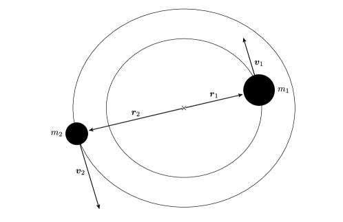
Figure B.1: Diagram of a binary system.

To solve the equation of motion of the two body problem it is useful to rewrite the equations in terms of relative quantities, like the spatial separation $\tvec{r}$, and relative velocity $\tvec{v}\equiv\dot{\tvec{r}}$. This will be done for the centre of mass frame in this appendix.

Letting $\tvec{r}_{i}$, $i\in\{1,2\}$ be the position of object $i$ relative the centre of mass, which is placed in the origin, as in Figure B.1 the following identity holds

$$\tvec{r}\equiv\tvec{r}_{2}-\tvec{r}_{1},$$ (B.1)

$$\begin{split}\tvec{0}\equiv\hskip 3.0pt&(m_{1}+m_{2})\tvec{R}_{\text{CM}}=m_{1}\tvec{r}_{1}+m_{2}\tvec{r}_{2},\\ \Rightarrow\quad&m_{1}\tvec{r}_{1}=-m_{2}\tvec{r}_{2}=-m_{2}\left(\tvec{r}+\tvec{r}_{1}\right).\end{split}$$ (B.2)

In the last line of (B.2) equation (B.1) was used to eliminate $\tvec{r}_{2}$. Similarly $\tvec{r}_{1}$ can be eliminated in favour of $\tvec{r}_{2}$. Thus $\tvec{r}_{i}$ can be expressed as

$$\tvec{r}_{1}=- \frac{m_{2}}{m_{1}+m_{2}}\tvec{r}=-\frac{m_{2}}{M}\tvec{r},$$ (B.3a)

$$\tvec{r}_{2}=\hskip 3.0pt \frac{m_{1}}{m_{1}+m_{2}}\tvec{r}=\frac{m_{1}}{M}\tvec{r}.$$ (B.3b)

Here $M$ is the total mass of the binary. Since the velocity of each object in the centre of mass frame is $\tvec{v}_{i}=\dot{\tvec{r}}_{i}$ it directly follows

$$\tvec{v}_{1}= -\frac{m_{2}}{M}\tvec{v},$$ (B.4a)

$$\tvec{v}_{2}= \hskip 3.0pt\frac{m_{1}}{M}\tvec{v},$$ (B.4b)

where again $\tvec{v}=\dot{\tvec{r}}$.

Substituting $\tvec{r}_{i}$ and $\tvec{v}_{i}$ for the expressions of equations (B.3)-(B.4) the Lagrangian, and thus the EoM, becomes a function of just $\tvec{r}$ and $\tvec{v}$. Thus the two body problem is reduced to solving for just the relative motion of one object, an equivalent one body problem.

Explicitly the Newtonian Lagrangian becomes

$$L\ind{{}_{\text{Newt}}} =\frac{1}{2}\left(m_{1}v_{1}^{2}+m_{2}v_{2}^{2}\right)+\frac{Gm_{1}m_{2}}{\absolutevalue{\tvec{r}_{2}-\tvec{r}_{1}}}=\frac{1}{2}\left(m_{1}\frac{m_{2}^{2}}{M^{2}}+m_{2}\frac{m_{1}^{2}}{M^{2}}\right)v^{2}+\frac{Gm_{1}m_{2}}{r}$$

$$=\frac{1}{2}\frac{m_{1}m_{2}}{M}\left(\frac{m_{2}+m_{1}}{M}\right)v^{2}+\frac{GM\frac{m_{1}m_{2}}{M}}{r}=\frac{1}{2}\frac{m_{1}m_{2}}{M}v^{2}+\frac{GM\frac{m_{1}m_{2}}{M}}{r}$$

$$\equiv\frac{1}{2}\mu v^{2}+\frac{GM\mu}{r}.$$

Bottom line is that preforming the substitution to $r$ and $v$ reduces the problem to describing the motion of one particle with an effective mass of $\mu=\frac{m_{1}m_{2}}{M}$ in a gravitational potential produced by an effective mass of $M=m_{1}+m_{2}$, which is static and located at the position of the other particle.

B.2 Mass term manipulation

Following the previous section it is hopefully clear what motivates the introduction of the total and reduced mass $M$ and $\mu$. The name reduced mass follows from the observation that in the extreme mass ratio, $m_{1}\gg m_{2}$, $M=m_{1}+m_{2}\simeq m_{1}$ and $\mu=\frac{m_{1}m_{2}}{M}\simeq\frac{m_{1}m_{2}}{m_{1}}=m_{2}$. I.e. in the test mass regime $M$ is the gravitational source and $\mu$ is the test mass exactly. Of course $M>\mu$ in all cases, with the largest value of $\mu_{\text{max}}=\frac{1}{4}M$ when $m_{1}=m_{2}$.

Moving beyond the Newtonian approximation there will appear other mass terms that are common in the literature. These are listen for convenience in equation (B.5).

In this thesis there will appear terms of the form $m_{1}v_{1}^{n+1}+m_{2}v_{2}^{n+1}$ and $m_{1}(-r_{1})^{n+1}+m_{2}r_{2}^{n+1}$. In this section there will be tips for strategies to convert these expressions into (B.5) type mass terms. The result can be read of equations (B.6)-(B.7).

$$M \equiv m_{1}+m_{2}$$ Total mass (B.5a)

$$\mu \equiv\frac{m_{1}m_{2}}{m_{1}+m_{2}}=\frac{m_{1}m_{2}}{M}$$ Reduced mass (B.5b)

$$\eta \equiv\frac{m_{1}m_{2}}{\left(m_{1}+m_{2}\right)^{2}}=\frac{\mu}{M}$$ Symmetric mass ratio (B.5c)

$$\M \equiv\frac{\left(m_{1}m_{2}\right)^{3/5}}{\left(m_{1}+m_{2}\right)^{1/5}}=\left(\mu^{3}M^{2}\right)^{1/5}=M\eta^{3/5}$$ Chirp mass (B.5d)

Here is a stepwise approach to deal with $m_{1}v_{1}^{n+1}+m_{2}v_{2}^{n+1}$ and $m_{1}(-r_{1})^{n+1}+m_{2}r_{2}^{n+1}$ type expressions.

1. The product $m_{1}m_{2}=M\mu$. Identify and extract all common factors of $\mu$ from the expression.

2. This will leave something like $\left(m_{2}^{n}\pm m_{1}^{n}\right)/M^{n}$.

   1. If it is a sum, calculate $M^{n}=m_{1}^{n}+m_{2}^{n}+\dots$. Thus $m_{2}^{n}+m_{1}^{n}=M^{n}-\dots$ Then again look out for reduced masses and remember that $\mu/M=\eta$.

   2. If it is a difference this will usually imply that $n$ is even. Let $n=2k$ and then $m_{2}^{2k}-m_{1}^{2k}=(m_{2}^{k}-m_{1}^{k})(m_{2}^{k}+m_{1}^{k})$. The $(m_{2}^{k}+m_{1}^{k})$ term can be expanded as in step 2a, and hopefully this will be enough. The difference can be further expanded using $m_{1}^{k}-m_{2}^{k}=\sqrt{(m_{1}^{k}-m_{2}^{k})^{2}}$ to get mixed terms which can be factored as $\mu$.

To get some concrete examples, lets consider $(m_{1}m_{2}^{4}+m_{2}m_{1}^{4})/M^{4}$.

$$\frac{m_{1}m_{2}^{4}+m_{2}m_{1}^{4}}{M^{4}} =\frac{m_{1}m_{2}}{M}\frac{m_{2}^{3}+m_{1}^{3}}{M^{3}}=\mu\frac{M^{3}-3m_{1}m_{2}(m_{1}+m_{2})}{M^{3}}$$

$$=\mu\left(1-3\mu/M\right)=\mu\left(1-3\eta\right).$$

$m_{2}^{3}+m_{1}^{3}$ was rewritten using equation (B.6c).

Most of the expressions encountered at 1PN will follow the same approach as the example above, with the exception of a term $(m_{2}m_{1}^{3}-m_{1}m_{2}^{3})/M^{3}$ which appear in the octupole moment of the flux (see LABEL:chap:flux). It goes like this

$$\frac{m_{2}m_{1}^{3}-m_{1}m_{2}^{3}}{M^{3}} =\mu\frac{m_{1}^{2}-m_{2}^{2}}{M^{2}}=\mu\frac{(m_{1}-m_{2})(m_{1}+m_{2})}{M^{2}}=\mu\frac{m_{1}-m_{2}}{M}$$

$$=\mu\sqrt{\frac{(m_{1}-m_{2})^{2}}{M^{2}}}=\mu\sqrt{\frac{m_{1}^{2}+m_{2}^{2}-2m_{1}m_{2}}{M^{2}}}=\mu\sqrt{\frac{M^{2}-4M\mu}{M^{2}}}$$

$$=\mu\sqrt{1-4\eta}.$$

In equation (B.6) the different sum of powers are listed, and in (B.7) the mixed products are listed. These expressions are useful for mass term manipulations like those that appear in this thesis.

$$m_{1}+m_{2} =M,$$ (B.6a)

$$m_{1}^{2}+m_{2}^{2} =M^{2}-2m_{1}m_{2}=M^{2}-2M\mu,$$ (B.6b)

$$m_{1}^{3}+m_{2}^{3} =M^{3}-3m_{1}^{2}m_{2}-3m_{1}m_{2}^{2}=M^{3}-3M^{2}\mu,$$ (B.6c)

$$\begin{split}m_{1}^{4}+m_{2}^{4}&=M^{4}-4m_{1}^{3}m_{2}-6m_{1}^{2}m_{2}^{2}-4m_{1}m_{2}^{3}\\ &=M^{4}+8M\mu^{2}-4M^{2}\mu-6M^{2}\mu^{2}.\end{split}$$ (B.6d)

$$m_{1}m_{2} =M\mu,$$ (B.7a)

$$m_{1}m_{2}^{2}+m_{1}^{2}m_{2} =M^{2}\mu,$$ (B.7b)

$$m_{1}m_{2}^{3}-m_{1}^{3}m_{2} =M^{3}\mu\sqrt{1-4\eta},$$ (B.7c)

$$m_{1}m_{2}^{4}+m_{1}^{4}m_{2} =M^{4}\mu\left(1-3\eta\right).$$ (B.7d)

A handy trick is to combine equation (B.7a) with expressions from (B.6) to obtain (B.7)-type expressions.

Appendix C Trigonometric identities

The trigonometric identities that are used in this thesis can all be derived using Euler’s formula

$$e^{i\theta}=\cos(\theta)+i\sin(\theta).$$ (C.1)

For the squared trigonometric functions one only needs to square this formula

$$\left(e^{i\theta}\right)^{2} =e^{i2\theta}=\cos(2\theta)+i\sin(2\theta)$$

$$=\left(\cos(\theta)+i\sin(\theta)\right)^{2}=\cos[2](\theta)-\sin[2](\theta)+i2\sin(\theta)\cos(\theta)$$

$$=2\cos[2](\theta)-1+i2\sin(\theta)\cos(\theta)=1-2\sin[2](\theta)+i2\sin(\theta)\cos(\theta),$$

where in the last line the Pythagorean identity $\sin[2](\theta)+\cos[2](\theta)=1$ was used to write the expression only by second powers in cosine or sine respectively. Comparing the real parts and imaginary parts of the first and third line produces the useful identities

$$\cos[2](\theta) =\frac{1}{2}\left(1+\cos(2\theta)\right),$$ (C.2a)

$$\sin[2](\theta) =\frac{1}{2}\left(1-\cos(2\theta)\right),$$ (C.2b)

$$\sin(\theta) \cos(\theta)=\frac{1}{2}\sin(2\theta).$$ (C.2c)

Likewise the identities for the third power trigonometric functions can be obtained

$$\left(e^{i\theta}\right)^{3} =e^{i3\theta}=\cos(3\theta)+i\sin(3\theta)=\left(\cos(\theta)+i\sin(\theta)\right)^{3}$$

$$=\cos[3](\theta)-3\cos(\theta)\sin[2](\theta)+i3\cos[2](\theta)\sin(\theta)-i\sin[3](\theta)$$

$$=\left[4\cos[3](\theta)-3\cos(\theta)\right]+i\left[3\sin(\theta)-4\sin[3](\theta)\right],$$

and then once again comparing the imaginary part of the first and third line the following identities are obtained.

$$\cos[3](\theta) =\frac{1}{4}\left(3\cos(\theta)+\cos(3\theta)\right),$$ (C.3a)

$$\sin[3](\theta) =\frac{1}{4}\left(3\sin(\theta)-\sin(3\theta)\right).$$ (C.3b)

References

- [1] B.. Abbott et al. “Observation of Gravitational Waves from a Binary Black Hole Merger” In Phys. Rev. Lett. 116 American Physical Society, 2016 DOI: 10.1103/PhysRevLett.116.061102
- [2] Herbert Goldstein, Charles Poole and John Safko “Classical Mechanics (3rd Edition)” Pearson Education Limited, 2014
- [3] Walter D. Goldberger and Ira Z. Rothstein “Effective field theory of gravity for extended objects” In Physical Review D 73.10 American Physical Society (APS), 2006 DOI: 10.1103/physrevd.73.104029
- [4] J. Blümlein, A. Maier, P. Marquard and G. Schäfer “The 6th post-Newtonian potential terms at ” In Phys. Lett. B 816, 2021, pp. 136260 DOI: 10.1016/j.physletb.2021.136260
- [5] J. Blümlein, A. Maier, P. Marquard and G. Schäfer “Testing binary dynamics in gravity at the sixth post-Newtonian level” In Phys. Lett. B 807, 2020, pp. 135496 DOI: 10.1016/j.physletb.2020.135496
- [6] J. Blümlein, A. Maier, P. Marquard and G. Schäfer “The fifth-order post-Newtonian Hamiltonian dynamics of two-body systems from an effective field theory approach”, 2021 arXiv:2110.13822 [gr-qc]
- [7] J. Blümlein, A. Maier, P. Marquard and G. Schäfer “The fifth-order post-Newtonian Hamiltonian dynamics of two-body systems from an effective field theory approach: potential contributions” In Nucl. Phys. B 965, 2021, pp. 115352 DOI: 10.1016/j.nuclphysb.2021.115352
- [8] J. Blümlein, A. Maier, P. Marquard and G. Schäfer “Fourth post-Newtonian Hamiltonian dynamics of two-body systems from an effective field theory approach” In Nucl. Phys. B 955, 2020, pp. 115041 DOI: 10.1016/j.nuclphysb.2020.115041
- [9] J. Blümlein, A. Maier, P. Marquard, G. Schäfer and C. Schneider “From Momentum Expansions to Post-Minkowskian Hamiltonians by Computer Algebra Algorithms” In Phys. Lett. B 801, 2020, pp. 135157 DOI: 10.1016/j.physletb.2019.135157
- [10] J. Blümlein, A. Maier and P. Marquard “Five-Loop Static Contribution to the Gravitational Interaction Potential of Two Point Masses” In Phys. Lett. B 800, 2020, pp. 135100 DOI: 10.1016/j.physletb.2019.135100
- [11] Rafael A. Porto “The effective field theorist’s approach to gravitational dynamics” In Physics Reports 633 Elsevier BV, 2016, pp. 1–104 DOI: 10.1016/j.physrep.2016.04.003
- [12] K.. Arun, Alessandra Buonanno, Guillaume Faye and Evan Ochsner “Higher-order spin effects in the amplitude and phase of gravitational waveforms emitted by inspiraling compact binaries: Ready-to-use gravitational waveforms” [Erratum: Phys.Rev.D 84, 049901 (2011)] In Phys. Rev. D 79, 2009 DOI: 10.1103/PhysRevD.79.104023
- [13] László B. Szabados “Quasi-Local Energy-Momentum and Angular Momentum in General Relativity” In Living Reviews in Relativity 12.4, 2009 DOI: https://doi.org/10.12942/lrr-2009-4
- [14] Sebastian De Haro “Noether’s Theorems and Energy in General Relativity”, 2021 arXiv:2103.17160 [physics.hist-ph]
- [15] Ssohrab Borhanian, K.. Arun, Harald P. Pfeiffer and B.. Sathyaprakash “Comparison of post-Newtonian mode amplitudes with numerical relativity simulations of binary black holes” In Class. Quant. Grav. 37.6, 2020, pp. 065006 DOI: 10.1088/1361-6382/ab6a21
- [16] Michele Maggiore “Gravitational Waves. Vol. 1: Theory and Experiments”, Oxford Master Series in Physics Oxford University Press, 2007 DOI: 10.1093/acprof:oso/9780198570745.001.0001
- [17] Stefano Foffa “Gravitating binaries at 5PN in the post-Minkowskian approximation” In Physical Review D 89, 2013 DOI: 10.1103/PhysRevD.89.024019
- [18] Curt Cutler and Eanna E. Flanagan “Gravitational waves from merging compact binaries: How accurately can one extract the binary’s parameters from the inspiral wave form?” In Phys. Rev. D 49, 1994, pp. 2658–2697 DOI: 10.1103/PhysRevD.49.2658
- [19] R.P. Feynman “Feynman lectures on gravitation”, 1996 DOI: 10.1201/9780429502859
- [20] Marco Di Mauro, Salvatore Esposito and Adele Naddeo “A roadmap for Feynman’s adventures in the land of gravitation”, 2021 arXiv:2102.11220 [physics.hist-ph]
- [21] M. Fierz and W. Pauli “On relativistic wave equations for particles of arbitrary spin in an electromagnetic field” In Proc. Roy. Soc. Lond. A 173, 1939, pp. 211–232 DOI: 10.1098/rspa.1939.0140
- [22] Éric Gourgoulhon “Special Relativity in General Frames”, Graduate Texts in Physics Berlin Heidelberg: Springer-Verlag, 2013 DOI: 10.1007/978-3-642-37276-6
- [23] Jakob Schwichtenberg “No-Nonsense Quantum Field Theory: A Student-Friendly Introduction” No-Nonsense Books, 2020 URL: https://nononsensebooks.com/qft/
- [24] Michael Kachelrieß “Quantum Fields: From the Hubble to the Planck Scale”, Oxford Graduate Texts Oxford University Press, 2017 DOI: 10.1093/oso/9780198802877.001.0001
- [25] Øyvind Grøn and Sigbjør Hervik “Einstein’s General Theory of Relativity” New York: Springer-Verlag, 2007 DOI: 10.1007/978-0-387-69200-5
- [26] Walter Goldberger “Les Houches Lectures on Effective Field Theories and Gravitational Radiation”, 2007 arXiv:hep-ph/0701129
- [27] T. Padmanabhan “FROM GRAVITONS TO GRAVITY: MYTHS AND REALITY” In International Journal of Modern Physics D 17.03n04 World Scientific Pub Co Pte Lt, 2008 DOI: 10.1142/s0218271808012085
- [28] R.. Feynman “Space-Time Approach to Quantum Electrodynamics” In Phys. Rev. 76 American Physical Society, 1949, pp. 769–789 DOI: 10.1103/PhysRev.76.769
- [29] L. Page and N.I. Adams “Electrodynamics”, Dover books on physics and mathematical physics D. Van Nostrand Company, Incorporated, 1940 URL: https://books.google.no/books?id=o7%5C_VAAAAMAAJ
- [30] A. Einstein, L. Infeld and B. Hoffmann “The Gravitational Equations and the Problem of Motion” In Annals of Mathematics 39.1 Annals of Mathematics, 1938, pp. 65–100 URL: http://www.jstor.org/stable/1968714
- [31] Graham Woan “The Cambridge Handbook of Physics Formulas” Cambridge University Press, 2000 DOI: 10.1017/CBO9780511755828
- [32] J… Battat, T.. Murphy, E.. Adelberger, B. Gillespie, C.. Hoyle, R.. McMillan, E.. Michelsen, K. Nordtvedt, A.. Orin, C.. Stubbs and H.. Swanson “The Apache Point Observatory Lunar Laser-ranging Operation (APOLLO): Two Years of Millimeter-Precision Measurements of the Earth-Moon Range1” In Publications of the Astronomical Society of the Pacific 121.875 IOP Publishing, 2009, pp. 29–40 DOI: 10.1086/596748
- [33] Ryan S. Park, William M. Folkner, James G. Williams and Dale H. Boggs “The JPL Planetary and Lunar Ephemerides DE440 and DE441” In The Astronomical Journal 161.3 American Astronomical Society, 2021, pp. 105 DOI: 10.3847/1538-3881/abd414
- [34] Andreas Ross “Multipole expansion at the level of the action” In Physical Review D 85, 2012 DOI: 10.1103/PhysRevD.85.125033
- [35] T. Damour and B.. Iyer “Multipole analysis for electromagnetism and linearized gravity with irreducible Cartesian tensors” In Phys. Rev. D 43 American Physical Society, 1991, pp. 3259–3272 DOI: 10.1103/PhysRevD.43.3259
- [36] Kip S. Thorne “Multipole expansions of gravitational radiation” In Rev. Mod. Phys. 52 American Physical Society, 1980, pp. 299–339 DOI: 10.1103/RevModPhys.52.299
- [37] Luc Blanchet “Gravitational Radiation from Post-Newtonian Sources and Inspiralling Compact Binaries” In Living Reviews in Relativity 17, 2014 DOI: 10.12942/lrr-2014-2
- [38] Richard Feynman “The Character of Physical Law” The MIT Press, 2017 DOI: https://doi.org/10.7551/mitpress/11068.001.0001
- [39] N. J. Bjerrum-Bohr, Poul H. Damgaard, Ludovic Planté and Pierre Vanhove “Classical Gravity from Loop Amplitudes”, 2021 arXiv:2104.04510 [hep-th]