Nonparametric Estimation for I.I.D. Paths of a Martingale Driven Model with Application to Non-Autonomous Financial Models

Abstract

This paper deals with a projection least squares estimator of the function $J_{0}$ computed from multiple independent observations on $[0,T]$ of the process $Z$ defined by $dZ_{t}=J_{0}(t)d\langle M\rangle_{t}+dM_{t}$, where $M$ is a continuous and square integrable martingale vanishing at $0$. Risk bounds are established on this estimator, on an associated adaptive estimator and on an associated discrete-time version used in practice. An appropriate transformation allows to rewrite the differential equation $dX_{t}=V(X_{t})(b_{0}(t)dt+\sigma(t)dB_{t})$, where $B$ is a fractional Brownian motion of Hurst parameter $H\in[1/2,1)$, as a model of the previous type. So, the second part of the paper deals with risk bounds on a nonparametric estimator of $b_{0}$ derived from the results on the projection least squares estimator of $J_{0}$. In particular, our results apply to the estimation of the drift function in a non-autonomous Black-Scholes model and to nonparametric estimation in a non-autonomous fractional stochastic volatility model.

JEL classification: C22

1 Introduction

Since the 1980’s, the statistical inference for stochastic differential equations (SDE) driven by a Brownian motion has been widely investigated by many authors in the parametric and in the nonparametric frameworks. Classically, the estimators of the drift function are computed from one path of the solution to the SDE and converge when the time horizon $T>0$ goes to infinity. The existence and the uniqueness of the stationary solution to the SDE are then required, and obtained thanks to restrictive conditions on the drift function. On such estimation methods, the reader can refer to Hoffmann HOFFMANN99 on a discrete-time wavelet based estimator, to Kutoyants KUTOYANTS04 (see Section 1.3.2 and Chapter 4) and Dalalyan DALALYAN05 on continuous-time kernel based estimators, to Comte et al. CGCR07 on a continuous-time projection least squares estimator, etc. Since few years, a new type of parametric and nonparametric estimators is investigated; those computed from multiple independent observations on $[0,T]$ of the SDE solution. On such estimation methods in the parametric framework, the reader can refer to Ditlevsen and De Gaetano DDG05 on a discrete-time maximum likelihood estimator of the drift parameter for SDE models with random effects, to Picchini, De Gaetano and Ditlevsen PDGD10 on an approximate maximum likelihood procedure for the estimation of both non-random parameters and the random effects, to Delattre and Lavielle DL13 on the SAEM algorithm combined with the extended Kalman filter to estimate the population parameters, to Delattre, Genon-Catalot and Larédo DGCL13 on a discrete-time approximate maximum likelihood estimator of random effects in the drift and in the diffusion coefficients, etc. In the nonparametric framework, some copies based estimation methods of the drift function have been recently investigated. Precisely, the reader can refer to Comte and Genon-Catalot CGC20b ; CGC21 on a continuous-time projection least squares estimator extended from nonparametric regression (see Cohen et al. CDL13 , Comte and Genon-Catalot CGC20a , etc.) to diffusion processes, to Della Maestra and Hoffmann DMH21 on a continuous-time Nadaraya-Watson estimator in interacting particle systems, to Denis et al. DDM21 on a discrete-time nonparametric ridge estimator, to Marie and Rosier MR21 on both continuous-time and discrete-time versions of a Nadaraya-Watson estimator with a PCO bandwidths selection method, etc. Our paper deals with a nonparametric estimation problem of similar kind.

Consider the stochastic process $Z=(Z_{t})_{t\in[0,T]}$, defined by

$$Z_{t}=\int_{0}^{t}J_{0}(s)d\langle M\rangle_{s}+M_{t}\textrm{$;$ }\forall t\in[0,T],$$ (1)

where $M=(M_{t})_{t\in[0,T]}\not=0$ is a continuous and square integrable martingale vanishing at $0$, and $J_{0}$ is an unknown function which almost surely belongs to $\mathbb{L}^{2}([0,T],d\langle M\rangle_{t})$. Under these conditions on $M$ and $J_{0}$, the quadratic variation $\langle M\rangle_{t}$ of $M$ is well-defined for any $t\in[0,T]$, and the Riemann-Stieljès integral of $J_{0}$ with respect to $s\mapsto\langle M\rangle_{s}$ on $[0,t]$ exists and is finite. So, the existence and the uniqueness of the process $Z$ are ensured. By assuming that $\langle M\rangle_{t}$ is deterministic for every $t\in[0,T]$, our paper deals with the estimator $\widehat{J}_{m,N}$ of $J_{0}$ minimizing the objective function

$$J\longmapsto\gamma_{N}(J):=\frac{1}{N}\sum_{i=1}^{N}\left(\int_{0}^{T}J(s)^{2}d\langle M^{i}\rangle_{s}-2\int_{0}^{T}J(s)dZ_{s}^{i}\right)$$

on a $m$-dimensional function space $\mathcal{S}_{m}$, where $M^{1},\dots,M^{N}$ (resp. $Z^{1},\dots,Z^{N}$) are $N\in\mathbb{N}^{*}$ independent copies of $M$ (resp. $Z$) and $m\in\{1,\dots,N\}$. Precisely, risk bounds are established on $\widehat{J}_{m,N}$ and on the adaptive estimator $\widehat{J}_{\widehat{m},N}$, where

$$\widehat{m}=\arg\min_{m\in\mathcal{M}_{N}}\{\gamma_{N}(\widehat{J}_{m,N})+{\rm pen}(m)\}$$

with $\mathcal{M}_{N}\subset\{1,\dots,N\}$,

$${\rm pen}(m):=\mathfrak{c}_{\rm cal}\frac{m}{N}\textrm{$;$ }\forall m\in\mathbb{N}$$

and $\mathfrak{c}_{\rm cal}>0$ is a constant to calibrate in practice. Now, consider the differential equation

$$X_{t}=X_{0}+\int_{0}^{t}V(X_{s})(b_{0}(s)ds+\sigma(s)dB_{s})\textrm{$;$ }t\in[0,T],$$ (2)

where $X_{0}$ is a $\mathbb{R}\backslash\{0\}$-valued random variable, $B=(B_{t})_{t\in[0,T]}$ is a fractional Brownian motion of Hurst parameter $H\in[1/2,1)$, the stochastic integral with respect to $B$ is taken pathwise (in Young’s sense) when $H>1/2$ and in Itô’s sense when $H=1/2$, and $V:\mathbb{R}\rightarrow\mathbb{R}$, $\sigma:[0,T]\rightarrow\mathbb{R}\backslash\{0\}$ and $b_{0}:[0,T]\rightarrow\mathbb{R}$ are at least continuous. An appropriate transformation (see Subsection 4.1) allows to rewrite Equation (2) as a model of type (1) driven by the Molchan martingale which quadratic variation is $t^{2-2H}$ for every $t\in[0,T]$. So, our paper also deals with a risk bound on an estimator of $b_{0}/\sigma$ derived from $\widehat{J}_{m,N}$. Up to our knowledge, only Comte and Marie CM21 deals with a nonparametric estimator of the drift function computed from multiple independent observations on $[0,T]$ of the solution to a fractional SDE. Finally, applications in mathematical finance are provided. On the one hand, an estimator of the drift function in a non-autonomous Black-Scholes model is given at Subsection 4.3. On the other hand, let us consider the fractional stochastic volatility model

$$\left\{\begin{array}[]{rcl}dS_{t}&=&S_{t}(b(t)dt+\sigma_{t}dW_{t})\\ d\sigma_{t}&=&\sigma_{t}(\rho_{0}(t)dt+\upsilon dB_{t})\end{array}\right.$$ (3)

where $S_{0}$ and $\sigma_{0}$ are $(0,\infty)$-valued random variables, $W=(W_{t})_{t\in[0,T]}$ is a Brownian motion, $\upsilon>0$ and $b,\rho_{0}\in C^{0}(\mathbb{R}_{+};\mathbb{R})$. This is a non-autonomous extension, with fractional volatility, of the stochastic volatility model studied in Wiggins WIGGINS87 . To take $H\in[1/2,1)$ allows to take into account the persistance in volatility phenomenon (see Comte et al. CCR12 ). An estimator of $\rho_{0}$ is given at Subsection 4.4.

At Section 2, a detailed definition of the projection least squares estimator of $J_{0}$ is provided. Section 3 deals with risk bounds on $\widehat{J}_{m,N}$, on the adaptive estimator $\widehat{J}_{\widehat{m},N}$ and on a discrete-time version of $\widehat{J}_{m,N}$ used in practice. At Section 4, the results of Section 3 on the estimator of $J_{0}$ are applied to the estimation of $b_{0}$ in Equation (2) and then to the estimator of the drift function (resp. $\rho_{0}$) in the non-autonomous Black-Scholes model (resp. in Equation (3)). Finally, some numerical experiments are provided at Section 5; in Model (1) when $M$ is the Molchan martingale, and in the non-autonomous Black-Scholes model.

Notations:

• $\langle.,.\rangle_{2,m}$ is the usual scalar product on $\mathbb{R}^{m}$, and $\|.\|_{2,m}$ is the associated norm.

• $\|.\|_{\rm op}$ is the spectral norm on the space $\mathcal{M}_{m}(\mathbb{R})$ of $m\times m$ real matrices.

• For any $p\geqslant 1$, the usual norm on $\mathbb{L}^{p}([0,T],dt)$ is denoted by $\|.\|_{p}$.

• For every closed and convex subset $C$ of a Hilbert space $H$, $p_{C}^{\perp}(.)$ is the orthogonal projection from $H$ onto $C$.

• For every bounded function $\varphi:[0,T]\rightarrow\mathbb{R}$,

  $$\|\varphi\|_{\infty,T}:=\sup_{t\in[0,T]}|\varphi(t)|.$$

• For any finite set $E$, $|E|$ is its cardinality.

2 A projection least squares estimator of the map $J_{0}$

In the sequel, the quadratic variation $\langle M\rangle=(\langle M\rangle_{t})_{t\in[0,T]}$ of $M$ fulfills the following assumption.

Assumption 2.1

The (nonnegative, increasing and continuous) process $\langle M\rangle$ is a deterministic function.

Assumption 2.1 is fulfilled by the Brownian motion and, more generally, by any martingale $(M_{t})_{t\in[0,T]}$ such that

$$M_{t}=\int_{0}^{t}\zeta(s)dW_{s}\textrm{$;$ }\forall t\in[0,T],$$

where $W$ is a Brownian motion and $\zeta\in\mathbb{L}^{2}([0,T],dt)$. For some results, $\langle M\rangle$ fulfills the following stronger assumption.

Assumption 2.2

There exists $\mu\in C^{0}((0,T];\mathbb{R}_{+})$ such that $\mu(.)^{-1}$ is continuous from $[0,T]$ into $\mathbb{R}_{+}$, and such that

$$\langle M\rangle_{t}=\int_{0}^{t}\mu(s)ds\textrm{$;$ }\forall t\in[0,T].$$

Here again, Assumption 2.2 is fulfilled by the Brownian motion. Assumption 2.2 is also fulfilled by any martingale $(M_{t})_{t\in[0,T]}$ such that

$$M_{t}=\int_{0}^{t}\zeta(s)dW_{s}\textrm{$;$ }\forall t\in[0,T],$$

where $W$ is a Brownian motion, $\zeta\in C^{0}((0,T];\mathbb{R})$ and $\zeta(.)^{-1}$ is continuous from $[0,T]$ into $\mathbb{R}$. This last condition is satisfied, for instance, when $\zeta$ is a $(c,\infty)$-valued function with $c>0$, or when $\zeta(t)=t^{-\kappa}$ for every $t\in(0,T]$ ($\kappa>0$). For instance, let $M$ be the Molchan martingale defined by

$$M_{t}:=\int_{0}^{t}\ell(t,s)dB_{s}\textrm{$;$ }\forall t\in[0,T],$$

where $B$ is a fractional Brownian motion of Hurst parameter $H\in[1/2,1)$, and

$$\ell(t,s):=\mathfrak{c}_{H}s^{1/2-H}(t-s)^{1/2-H}\mathbf{1}_{(0,t)}(s)\textrm{$;$ }\forall s,t\in[0,T]$$

with

$$\mathfrak{c}_{H}=\left(\frac{\Gamma(3-2H)}{2H\Gamma(3/2-H)^{3}\Gamma(H+1/2)}\right)^{1/2}.$$

Since

$$M_{t}=(2-2H)^{1/2}\int_{0}^{t}s^{1/2-H}dW_{s}\textrm{$;$ }\forall t\in[0,T],$$

where $W$ is the Brownian motion driving the Mandelbrot-Van Ness representation of the fractional Brownian motion $B$, the Molchan martingale fulfills Assumption 2.2 with $\mu(t)=(2-2H)t^{1-2H}$ for every $t\in(0,T]$.

2.1 The objective function

In order to define a least squares projection estimator of $J_{0}$, let us consider $N\in\mathbb{N}^{*}$ independent copies $M^{1},\dots,M^{N}$ (resp. $Z^{1},\dots,Z^{N}$) of $M$ (resp. $Z$), and the objective function $\gamma_{N}$ defined by

$$\gamma_{N}(J):=\frac{1}{N}\sum_{i=1}^{N}\left(\int_{0}^{T}J(s)^{2}d\langle M^{i}\rangle_{s}-2\int_{0}^{T}J(s)dZ_{s}^{i}\right)$$

for every $J\in\mathcal{S}_{m}$, where $m\in\{1,\dots,N\}$, $\mathcal{S}_{m}:={\rm span}\{\varphi_{1},\dots,\varphi_{m}\}$ and $\varphi_{1},\dots,\varphi_{N}$ are continuous functions from $[0,T]$ into $\mathbb{R}$ such that $(\varphi_{1},\dots,\varphi_{N})$ is an orthonormal family in $\mathbb{L}^{2}([0,T],dt)$.

Remark. Note that since $t\in[0,T]\mapsto\langle M\rangle_{t}$ is nonnegative, increasing and continuous, and since the $\varphi_{j}$’s are continuous from $[0,T]$ into $\mathbb{R}$, the objective function $\gamma_{N}$ is well-defined.

For any $J\in\mathcal{S}_{m}$,

$$\mathbb{E}[\gamma_{N}(J)] = \int_{0}^{T}J(s)^{2}d\langle M\rangle_{s}-2\int_{0}^{T}J(s)J_{0}(s)d\langle M\rangle_{s}-2\mathbb{E}\left[\int_{0}^{T}J(s)dM_{s}\right]$$

$$= \int_{0}^{T}(J(s)-J_{0}(s))^{2}d\langle M\rangle_{s}-\int_{0}^{T}J_{0}(s)^{2}d\langle M\rangle_{s}.$$

Then, the more $J$ is close to $J_{0}$, the more $\mathbb{E}[\gamma_{N}(J)]$ is small. For this reason, the estimator of $J_{0}$ minimizing $\gamma_{N}$ is studied in this paper.

2.2 The projection least squares estimator

Consider

$$J:=\sum_{j=1}^{m}\theta_{j}\varphi_{j}\quad{\rm with}\quad\theta_{1},\dots,\theta_{m}\in\mathbb{R}.$$

Then,

$$\nabla\gamma_{N}(J) = \left(\frac{1}{N}\sum_{i=1}^{N}\left(2\sum_{k=1}^{m}\theta_{k}\int_{0}^{T}\varphi_{j}(s)\varphi_{k}(s)d\langle M^{i}\rangle_{s}-2\int_{0}^{T}\varphi_{j}(s)dZ_{s}^{i}\right)\right)_{j\in\{1,\dots,m\}}$$

$$= 2(\Psi_{m}(\theta_{1},\dots,\theta_{m})^{*}-z_{m,N})$$

where

$$\Psi_{m}:=\left(\int_{0}^{T}\varphi_{j}(s)\varphi_{k}(s)d\langle M\rangle_{s}\right)_{j,k\in\{1,\dots,m\}}\quad{\rm and}\quad z_{m,N}:=\left(\frac{1}{N}\sum_{i=1}^{N}\int_{0}^{T}\varphi_{j}(s)dZ_{s}^{i}\right)_{j\in\{1,\dots,m\}}.$$

Moreover, the symmetric matrix $\Psi_{m}$ is nonnegative because under Assumption 2.1,

$$u^{*}\Psi_{m}u=\int_{0}^{T}\left(\sum_{j=1}^{m}u_{j}\varphi_{j}(s)\right)^{2}d\langle M\rangle_{s}\geqslant 0$$

for every $u\in\mathbb{R}^{m}$. In fact, since $\varphi_{1},\dots,\varphi_{m}$ are linearly independent, $\Psi_{m}$ is even a positive-definite matrix, and thus $\gamma_{N}$ has a unique minimum in $\mathcal{S}_{m}$. This legitimates to consider the estimator

$$\widehat{J}_{m,N}=\arg\min_{J\in\mathcal{S}_{m}}\gamma_{N}(J)$$ (4)

of $J_{0}$, and since $\nabla\gamma_{N}(\widehat{J}_{m,N})=0$,

$$\widehat{J}_{m,N}=\sum_{j=1}^{m}\widehat{\theta}_{j}\varphi_{j}$$

with

$$\widehat{\theta}_{m,N}:=(\widehat{\theta}_{1},\dots,\widehat{\theta}_{m})^{*}=\Psi_{m}^{-1}z_{m,N}.$$

In practice, since the process $Z$ cannot be observed continuously on the time interval $[0,T]$, the vector $z_{m,N}$ has to be replaced by the approximation

$$z_{m,N,n}:=\left(\frac{1}{N}\sum_{i=1}^{N}\sum_{l=0}^{n-1}\varphi_{j}(t_{l})(Z_{t_{l+1}}^{i}-Z_{t_{l}}^{i})\right)_{j\in\{1,\dots,m\}}$$

in the definition of $\widehat{J}_{m,N}$, where $t_{l}:=lT/n$ for every $l\in\{0,\dots,n\}$. This leads to the discrete-time estimator

$$\widehat{J}_{m,N,n}:=\sum_{j=1}^{m}[\widehat{\theta}_{m,N,n}]_{j}\varphi_{j}\quad{\rm with}\quad\widehat{\theta}_{m,N,n}:=\Psi_{m}^{-1}z_{m,N,n}.$$

3 Risk bounds and model selection

In the sequel, the space $\mathbb{L}^{2}([0,T],d\langle M\rangle_{t})$ is equipped with the scalar product $\langle.,.\rangle_{\langle M\rangle}$ defined by

$$\langle\varphi,\psi\rangle_{\langle M\rangle}:=\int_{0}^{T}\varphi(s)\psi(s)d\langle M\rangle_{s}$$

for every $\varphi,\psi\in\mathbb{L}^{2}([0,T],d\langle M\rangle_{t})$. The associated norm is denoted by $\|.\|_{\langle M\rangle}$.

First, the following proposition provides a risk bound on $\widehat{J}_{m,N}$ for a fixed $m\in\{1,\dots,N\}$.

Proposition 1

Under Assumption 2.1,

$$\mathbb{E}[\|\widehat{J}_{m,N}-J_{0}\|_{\langle M\rangle}^{2}]\leqslant\min_{J\in\mathcal{S}_{m}}\|J-J_{0}\|_{\langle M\rangle}^{2}+\frac{2m}{N}.$$ (5)

Proof

For every $J,K\in\mathcal{S}_{m}$,

$$\gamma_{N}(J)-\gamma_{N}(K) = \|J\|_{\langle M\rangle}^{2}-\|K\|_{\langle M\rangle}^{2}-\frac{2}{N}\sum_{i=1}^{N}\int_{0}^{T}(J(s)-K(s))dZ_{s}^{i}$$

$$= \|J-J_{0}\|_{\langle M\rangle}^{2}-\|K-J_{0}\|_{\langle M\rangle}^{2}-\frac{2}{N}\sum_{i=1}^{N}\int_{0}^{T}(J(s)-K(s))dM_{s}^{i}.$$

Moreover,

$$\gamma_{N}(\widehat{J}_{m,N})\leqslant\gamma_{N}(J)\textrm{$;$ }\forall J\in\mathcal{S}_{m}.$$

So,

$$\|\widehat{J}_{m,N}-J_{0}\|_{\langle M\rangle}^{2}\leqslant\|J-J_{0}\|_{\langle M\rangle}^{2}+\frac{2}{N}\sum_{i=1}^{N}\int_{0}^{T}(\widehat{J}_{m,N}(s)-J(s))dM_{s}^{i}$$

for any $J\in\mathcal{S}_{m}$, and then

$$\mathbb{E}[\|\widehat{J}_{m,N}-J_{0}\|_{\langle M\rangle}^{2}]\leqslant\|J-J_{0}\|_{\langle M\rangle}^{2}+2\mathbb{E}\left[\frac{1}{N}\sum_{i=1}^{N}\int_{0}^{T}\widehat{J}_{m,N}(s)dM_{s}^{i}\right].$$

Consider $j_{0}=(\langle\varphi_{j},J_{0}\rangle_{\langle M\rangle})_{j=1,\dots,m}$, and $e=(e_{1},\dots,e_{m})^{*}$ such that

$$e_{j}:=\frac{1}{N}\sum_{i=1}^{N}\int_{0}^{T}\varphi_{j}(s)dM_{s}^{i}\textrm{$;$ }\forall j\in\{1,\dots,m\}.$$

Since $e$ is a centered random vector,

$$\mathbb{E}\left[\frac{1}{N}\sum_{i=1}^{N}\int_{0}^{T}\widehat{J}_{m,N}(s)dM_{s}^{i}\right] = \sum_{j=1}^{m}\mathbb{E}\left[\widehat{\theta}_{j}\cdot\frac{1}{N}\sum_{i=1}^{N}\int_{0}^{T}\varphi_{j}(s)dM_{s}^{i}\right]$$

$$= \mathbb{E}[\langle\widehat{\theta},e\rangle_{2,m}]=\mathbb{E}[e^{*}\Psi_{m}^{-1}(j_{0}+e)]=\mathbb{E}[e^{*}\Psi_{m}^{-1}e].$$

Moreover, since $M_{1},\dots,M_{N}$ are independent copies of $M$, and since $\Psi_{m}$ is a symmetric matrix,

$$\mathbb{E}[e^{*}\Psi_{m}^{-1}e] = \sum_{j,k=1}^{m}[\Psi_{m}^{-1}]_{j,k}\mathbb{E}[e_{j}e_{k}]=\frac{1}{N}\sum_{j,k=1}^{m}[\Psi_{m}^{-1}]_{j,k}\int_{0}^{T}\varphi_{j}(s)\varphi_{k}(s)d\langle M\rangle_{s}$$

$$= \frac{1}{N}\sum_{k=1}^{m}\sum_{j=1}^{m}[\Psi_{m}]_{k,j}[\Psi_{m}^{-1}]_{j,k}=\frac{1}{N}\sum_{k=1}^{m}[\Psi_{m}\Psi_{m}^{-1}]_{k,k}=\frac{m}{N}.$$

Therefore,

$$\mathbb{E}[\|\widehat{J}_{m,N}-J_{0}\|_{\langle M\rangle}^{2}]\leqslant\min_{J\in\mathcal{S}_{m}}\|J-J_{0}\|_{\langle M\rangle}^{2}+\frac{2m}{N}.\quad\qed$$

Note that Inequality (5) says first that the bound on the variance of our least squares estimator of $J_{0}$ is of order $m/N$, as in the usual nonparametric regression framework. Under Assumption 2.2, the following corollary provides a more understandable expression of the bound on the bias in Inequality (5).

Corollary 1

Under Assumption 2.2,

$$\mathbb{E}[\|\widehat{J}_{m,N}-J_{0}\|_{2}^{2}]\leqslant\|\mu(.)^{-1}\|_{\infty,T}\|p_{\mathcal{S}_{m}(\mu)}^{\perp}(\mu^{1/2}J_{0})-\mu^{1/2}J_{0}\|_{2}^{2}+2\|\mu(.)^{-1}\|_{\infty,T}\frac{m}{N}$$

where

$$\mathcal{S}_{m}(\mu):=\{\iota\in\mathbb{L}^{2}([0,T],dt):\exists\varphi\in\mathcal{S}_{m}\textrm{, }\forall t\in(0,T]\textrm{, }\iota(t)=\mu(t)^{1/2}\varphi(t)\}.$$

Proof

Under Assumption 2.2,

$$\min_{J\in\mathcal{S}_{m}}\|J-J_{0}\|_{\langle M\rangle}^{2}=\min_{J\in\mathcal{S}_{m}}\|\mu^{1/2}(J-J_{0})\|_{2}^{2}=\min_{\iota\in\mathcal{S}_{m}(\mu)}\|\iota-\mu^{1/2}J_{0}\|_{2}^{2}$$

with

$$\mathcal{S}_{m}(\mu)=\{\iota\in\mathbb{L}^{2}([0,T],dt):\exists\varphi\in\mathcal{S}_{m}\textrm{, }\forall t\in(0,T]\textrm{, }\iota(t)=\mu(t)^{1/2}\varphi(t)\}.$$

Since $\mathcal{S}_{m}(\mu)$ is a closed vector subspace of $\mathbb{L}^{2}([0,T],dt)$,

$$\min_{\iota\in\mathcal{S}_{m}(\mu)}\|\iota-\mu^{1/2}J_{0}\|_{2}^{2}=\|p_{\mathcal{S}_{m}(\mu)}^{\perp}(\mu^{1/2}J_{0})-\mu^{1/2}J_{0}\|_{2}^{2}.$$ (6)

Moreover, since $\mu(.)^{-1}$ is continuous from $[0,T]$ into $\mathbb{R}_{+}$ under Assumption 2.2,

$$\|\widehat{J}_{m,N}-J_{0}\|_{2}^{2} = \|\mu^{-1/2}(\widehat{J}_{m,N}-J_{0})\|_{\langle M\rangle}^{2}$$ (7)

$$\leqslant \|\mu(.)^{-1}\|_{\infty,T}\|\widehat{J}_{m,N}-J_{0}\|_{\langle M\rangle}^{2}.$$

Equality (6) together with Inequality (7) allow to conclude.∎

For instance, assume that $\mathcal{S}_{m}={\rm span}\{\overline{\varphi}_{1},\dots,\overline{\varphi}_{m}\}$, where

$$\overline{\varphi}_{1}(t):=\sqrt{\frac{1}{\mu(t)T}},\quad\overline{\varphi}_{2j}(t):=\sqrt{\frac{2}{\mu(t)T}}\cos\left(2\pi j\frac{t}{T}\right)\quad{\rm and}\quad\overline{\varphi}_{2j+1}(t):=\sqrt{\frac{2}{\mu(t)T}}\sin\left(2\pi j\frac{t}{T}\right)$$

for every $t\in[0,T]$ and $j\in\mathbb{N}^{*}$ satisfying $2j+1\leqslant m$. The basis $(\varphi_{1},\dots,\varphi_{m})$ of $\mathcal{S}_{m}$, orthonormal in $\mathbb{L}^{2}([0,T],dt)$, is obtained from $(\overline{\varphi}_{1},\dots,\overline{\varphi}_{m})$ via the Gram-Schmidt process. Consider also the Sobolev space

$$\mathbb{W}_{2}^{\beta}([0,T]):=\left\{\iota\in C^{\beta-1}([0,T];\mathbb{R}):\int_{0}^{T}\iota^{(\beta)}(t)^{2}dt<\infty\right\}\textrm{$;$ }\beta\in\mathbb{N}^{*},$$

and assume that there exists $\iota_{0}\in\mathbb{W}_{2}^{\beta}([0,T])$ such that $\iota_{0}(t)=\mu(t)^{1/2}J_{0}(t)$ for every $t\in(0,T]$. Then, by DeVore and Lorentz DL93 , Chapter 7, Corollary 2.4, there exists a constant $\mathfrak{c}_{\beta,T}>0$, not depending on $m$, such that

$$\|p_{\mathcal{S}_{m}(\mu)}^{\perp}(\mu^{1/2}J_{0})-\mu^{1/2}J_{0}\|_{2}^{2}=\|p_{\mathcal{S}_{m}(\mu)}^{\perp}(\iota_{0})-\iota_{0}\|_{2}^{2}\leqslant\mathfrak{c}_{\beta,T}m^{-2\beta}.$$

Therefore, by Corollary 1,

$$\mathbb{E}[\|\widehat{J}_{m,N}-J_{0}\|_{2}^{2}]\leqslant\|\mu(.)^{-1}\|_{\infty,T}\left(\mathfrak{c}_{\beta,T}m^{-2\beta}+\frac{2m}{N}\right).$$

Now, consider $m_{N}\in\{1,\dots,N\}$, $\mathcal{M}_{N}:=\{1,\dots,m_{N}\}$ and

$$\widehat{m}=\arg\min_{m\in\mathcal{M}_{N}}\{\gamma_{N}(\widehat{J}_{m,N})+{\rm pen}(m)\}\quad{\rm with}\quad{\rm pen}(.):=\mathfrak{c}_{\rm cal}\frac{.}{N},$$ (8)

where $\mathfrak{c}_{\rm cal}>0$ is a constant to calibrate in practice via, for instance, the slope heuristic. In the sequel, the $\varphi_{j}$’s fulfill the following assumption.

Assumption 3.1

For every $m,m^{\prime}\in\{1,\dots,N\}$, if $m>m^{\prime}$, then $\mathcal{S}_{m^{\prime}}\subset\mathcal{S}_{m}$.

The following theorem provides a risk bound on the adaptive estimator $\widehat{J}_{\widehat{m},N}$.

Theorem 3.2

Under Assumptions 2.1 and 3.1, there exists a deterministic constant $\mathfrak{c}_{\ref{risk_bound_adaptive_estimator}}>0$, not depending on $N$, such that

$$\mathbb{E}[\|\widehat{J}_{\widehat{m},N}-J_{0}\|_{\langle M\rangle}^{2}]\leqslant\mathfrak{c}_{\ref{risk_bound_adaptive_estimator}}\left(\min_{m\in\mathcal{M}_{N}}\{\mathbb{E}[\|\widehat{J}_{m,N}-J_{0}\|_{\langle M\rangle}^{2}]+{\rm pen}(m)\}+\frac{1}{N}\right).$$

Moreover, under Assumption 2.2,

$$\mathbb{E}[\|\widehat{J}_{\widehat{m},N}-J_{0}\|_{2}^{2}]\leqslant\mathfrak{c}_{\ref{risk_bound_adaptive_estimator}}\|\mu(.)^{-1}\|_{\infty,T}\left(\min_{m\in\mathcal{M}_{N}}\left\{\|p_{\mathcal{S}_{m}(\mu)}^{\perp}(\mu^{1/2}J_{0})-\mu^{1/2}J_{0}\|_{2}^{2}+(2+\mathfrak{c}_{\rm cal})\frac{m}{N}\right\}+\frac{1}{N}\right).$$

The proof of Theorem 3.2 relies on the following lemma, which is a straightforward consequence of a Bernstein type inequality for continuous local martingales vanishing at $0$ (see Revuz and Yor RY99 , Chapter IV, Exercice 3.16).

Lemma 1

For every $\varepsilon>0$ and every $\varphi\in\mathbb{L}^{2}([0,T],d\langle M\rangle_{t})$,

$$\mathbb{P}\left[\frac{1}{N}\sum_{i=1}^{N}\int_{0}^{T}\varphi(s)dM_{s}^{i}\geqslant\varepsilon\right]\leqslant\exp\left(-\frac{N\varepsilon^{2}}{2\|\varphi\|_{\langle M\rangle}^{2}}\right).$$

Let us establish Theorem 3.2.

Proof

of Theorem 3.2. Let us proceed in three steps.

Step 1. As established in the proof of Proposition 1, for every $J,K\in\mathcal{S}_{m}$,

$$\gamma_{N}(J)-\gamma_{N}(K)=\|J-J_{0}\|_{\langle M\rangle}^{2}-\|K-J_{0}\|_{\langle M\rangle}^{2}-\frac{2}{N}\sum_{i=1}^{N}\int_{0}^{T}(J(s)-K(s))dM_{s}^{i}.$$

Moreover,

$$\gamma_{N}(\widehat{J}_{\widehat{m},N})+{\rm pen}(\widehat{m})\leqslant\gamma_{N}(\widehat{J}_{m,N})+{\rm pen}(m)$$

for any $m\in\mathcal{M}_{N}$, and then

$$\gamma_{N}(\widehat{J}_{\widehat{m},N})-\gamma_{N}(\widehat{J}_{m,N})\leqslant{\rm pen}(m)-{\rm pen}(\widehat{m}).$$

So, since $\mathcal{S}_{m}+\mathcal{S}_{\widehat{m}}\subset\mathcal{S}_{m\vee\widehat{m}}$ under Assumption 3.1, and since $2ab\leqslant a^{2}+b^{2}$ for every $a,b\in\mathbb{R}$,

$$\|\widehat{J}_{\widehat{m},N}-J_{0}\|_{\langle M\rangle}^{2} \leqslant \|\widehat{J}_{m,N}-J_{0}\|_{\langle M\rangle}^{2}+\frac{2}{N}\sum_{i=1}^{N}\int_{0}^{T}(\widehat{J}_{\widehat{m},N}(s)-\widehat{J}_{m,N}(s))dM_{s}^{i}+{\rm pen}(m)-{\rm pen}(\widehat{m})$$

$$\leqslant \|\widehat{J}_{m,N}-J_{0}\|_{\langle M\rangle}^{2}+2\cdot\frac{1}{2}\|\widehat{J}_{\widehat{m},N}-\widehat{J}_{m,N}\|_{\langle M\rangle}\cdot 2\sup_{\varphi\in\mathcal{B}_{m,\widehat{m}}}|\nu_{N}(\varphi)|+{\rm pen}(m)-{\rm pen}(\widehat{m})$$

$$\leqslant \|\widehat{J}_{m,N}-J_{0}\|_{\langle M\rangle}^{2}+\frac{1}{4}\|\widehat{J}_{\widehat{m},N}-\widehat{J}_{m,N}\|_{\langle M\rangle}^{2}$$

$$\hskip 56.9055pt+4\left(\left[\sup_{\varphi\in\mathcal{B}_{m,\widehat{m}}}|\nu_{N}(\varphi)|\right]^{2}-p(m,\widehat{m})\right)_{+}+{\rm pen}(m)+4p(m,\widehat{m})-{\rm pen}(\widehat{m}),$$

where

$$\mathcal{B}_{m,m^{\prime}}:=\{\varphi\in\mathcal{S}_{m\vee m^{\prime}}:\|\varphi\|_{\langle M\rangle}=1\}\quad{\rm and}\quad p(m,m^{\prime}):=\frac{\mathfrak{c}_{\rm cal}}{4}\cdot\frac{m\vee m^{\prime}}{N}$$

for every $m^{\prime}\in\mathcal{M}_{N}$, and

$$\nu_{N}(\varphi):=\frac{1}{N}\sum_{i=1}^{N}\int_{0}^{T}\varphi(s)dM_{s}^{i}$$

for every $\varphi\in\mathbb{L}^{2}([0,T],d\langle M\rangle_{t})$. Therefore, since $(a+b)^{2}\leqslant 2a^{2}+2b^{2}$ for every $a,b\in\mathbb{R}$, and since $4p(m,\widehat{m})\leqslant{\rm pen}(m)+{\rm pen}(\widehat{m})$,

$$\|\widehat{J}_{\widehat{m},N}-J_{0}\|_{\langle M\rangle}^{2}\leqslant 3\|\widehat{J}_{m,N}-J_{0}\|_{\langle M\rangle}^{2}+4{\rm pen}(m)+8\left(\left[\sup_{\varphi\in\mathcal{B}_{m,\widehat{m}}}|\nu_{N}(\varphi)|\right]^{2}-p(m,\widehat{m})\right)_{+}.$$ (9)

Step 2. By using Lemma 1, and by following the pattern of the proof of Baraud et al. BCV07 , Proposition 6.1, the purpose of this step is to find a suitable bound on

$$\mathbb{E}\left[\left(\left[\sup_{\varphi\in\mathcal{B}_{m,m^{\prime}}}|\nu_{N}(\varphi)|\right]^{2}-p(m,m^{\prime})\right)_{+}\right]\textrm{$;$ }m^{\prime}\in\mathcal{M}_{N}.$$

Consider $\delta_{0}\in(0,1)$ and let $(\delta_{n})_{n\in\mathbb{N}^{*}}$ be the real sequence defined by

$$\delta_{n}:=\delta_{0}2^{-n}\textrm{$;$ }\forall n\in\mathbb{N}^{*}.$$

Since $\mathcal{S}_{m\vee m^{\prime}}$ is a vector subspace of $\mathbb{L}^{2}([0,T],d\langle M\rangle_{t})$ of dimension $m\vee m^{\prime}$, for any $n\in\mathbb{N}$, by Lorentz et al. LGM96 , Chapter 15, Proposition 1.3, there exists $T_{n}\subset\mathcal{B}_{m,m^{\prime}}$ such that $|T_{n}|\leqslant(3/\delta_{n})^{m\vee m^{\prime}}$ and, for any $\varphi\in\mathcal{B}_{m,m^{\prime}}$,

$$\exists f_{n}\in T_{n}:\|\varphi-f_{n}\|_{\langle M\rangle}\leqslant\delta_{n}.$$

In particular, note that

$$\varphi=f_{0}+\sum_{n=1}^{\infty}(f_{n}-f_{n-1}).$$

Then, for any sequence $(\Delta_{n})_{n\in\mathbb{N}}$ of elements of $(0,\infty)$ such that $\Delta:=\sum_{n\in\mathbb{N}}\Delta_{n}<\infty$,

$$\mathbb{P}\left[\left(\sup_{\varphi\in\mathcal{B}_{m,m^{\prime}}}|\nu_{N}(\varphi)|\right)^{2}>\Delta^{2}\right]$$

$$\hskip 56.9055pt=\mathbb{P}\left[\exists(f_{n})_{n\in\mathbb{N}}\in\prod_{n=0}^{\infty}T_{n}:|\nu_{N}(f_{0})|+\sum_{n=1}^{\infty}|\nu_{N}(f_{n}-f_{n-1})|>\Delta\right]$$

$$\hskip 56.9055pt\leqslant\mathbb{P}\left[\exists(f_{n})_{n\in\mathbb{N}}\in\prod_{n=0}^{\infty}T_{n}:|\nu_{N}(f_{0})|>\Delta_{0}\textrm{ or }[\exists n\in\mathbb{N}^{*}:|\nu_{N}(f_{n}-f_{n-1})|>\Delta_{n}]\right]$$

$$\hskip 56.9055pt\leqslant\sum_{f_{0}\in T_{0}}\mathbb{P}[|\nu_{N}(f_{0})|>\Delta_{0}]+\sum_{n=1}^{\infty}\sum_{(f_{n-1},f_{n})\in\mathbb{T}_{n}}\mathbb{P}[|\nu_{N}(f_{n}-f_{n-1})|>\Delta_{n}]$$

with $\mathbb{T}_{n}=T_{n-1}\times T_{n}$ for every $n\in\mathbb{N}^{*}$. Moreover, $\|f_{0}\|_{\langle M\rangle}^{2}\leqslant 1$ and

$$\|f_{n}-f_{n-1}\|_{\langle M\rangle}^{2}\leqslant 2\delta_{n-1}^{2}+2\delta_{n}^{2}=\frac{5}{2}\delta_{n-1}^{2}$$

for every $n\in\mathbb{N}^{*}$. So, by Lemma 1,

$$\mathbb{P}\left[\left(\sup_{\varphi\in\mathcal{B}_{m,m^{\prime}}}|\nu_{N}(\varphi)|\right)^{2}>\Delta^{2}\right] \leqslant 2\sum_{f_{0}\in T_{0}}\exp\left(-\frac{N\Delta_{0}^{2}}{2\|f_{0}\|_{\langle M\rangle}^{2}}\right)$$ (10)

$$\hskip 56.9055pt+2\sum_{n=1}^{\infty}\sum_{(f_{n-1},f_{n})\in\mathbb{T}_{n}}\exp\left(-\frac{N\Delta_{n}^{2}}{2\|f_{n}-f_{n-1}\|_{\langle M\rangle}^{2}}\right)$$

$$\leqslant 2\exp\left(h_{0}-\frac{N\Delta_{0}^{2}}{2}\right)+2\sum_{n=1}^{\infty}\exp\left(h_{n-1}+h_{n}-\frac{N\Delta_{n}^{2}}{5\delta_{n-1}^{2}}\right)$$

with $h_{n}=\log(|T_{n}|)$ for every $n\in\mathbb{N}$. Now, let us take $\Delta_{0}$ such that

$$h_{0}-\frac{N\Delta_{0}^{2}}{2}=-(m\vee m^{\prime}+x)\quad{\rm with}\quad x>0,$$

which leads to

$$\Delta_{0}=\left[\frac{2}{N}(m\vee m^{\prime}+x+h_{0})\right]^{1/2},$$

and for every $n\in\mathbb{N}^{*}$, let us take $\Delta_{n}$ such that

$$h_{n-1}+h_{n}-\frac{N\Delta_{n}^{2}}{5\delta_{n-1}^{2}}=-(m\vee m^{\prime}+x+n),$$

which leads to

$$\Delta_{n}=\left[\frac{5\delta_{n-1}^{2}}{N}(m\vee m^{\prime}+x+h_{n-1}+h_{n}+n)\right]^{1/2}.$$

For this appropriate sequence $(\Delta_{n})_{n\in\mathbb{N}}$,

$$\mathbb{P}\left[\left(\sup_{\varphi\in\mathcal{B}_{m,m^{\prime}}}|\nu_{N}(\varphi)|\right)^{2}>\Delta^{2}\right]\leqslant 2e^{-x}e^{-(m\vee m^{\prime})}\left(1+\sum_{n=1}^{\infty}e^{-n}\right)\leqslant 3.2e^{-x}e^{-(m\vee m^{\prime})}$$

by Inequality (10), and

$$\Delta^{2} \leqslant \frac{1}{N}\left[\sqrt{2}[(m\vee m^{\prime}+x)^{1/2}+h_{0}^{1/2}]+\sqrt{5}\sum_{n=1}^{\infty}\delta_{n-1}[(m\vee m^{\prime}+x)^{1/2}+(h_{n-1}+h_{n}+n)^{1/2}]\right]^{2}$$

$$\leqslant \frac{\delta^{(1)}}{N}(m\vee m^{\prime}+x)+\frac{\delta^{(2)}}{N}\leqslant\frac{\delta^{(1)}+\delta^{(2)}}{N}(m\vee m^{\prime}+x)$$

with

$$\delta^{(1)}=2\left(\sqrt{2}+\sqrt{5}\sum_{n=1}^{\infty}\delta_{n-1}\right)^{2},$$

$$\hskip 42.67912pt{\rm and}\quad\delta^{(2)}=2\left(\sqrt{2}h_{0}^{1/2}+\sqrt{5}\sum_{n=1}^{\infty}\delta_{n-1}\left[n+N_{T}\left(2\log\left(\frac{3}{\delta_{0}}\right)+(2n-1)\log(2)\right)\right]^{1/2}\right)^{2}$$

because

$$h_{n-1}+h_{n} \leqslant (m\vee m^{\prime})\left[\log\left(\frac{3}{\delta_{n-1}}\right)+\log\left(\frac{3}{\delta_{n}}\right)\right]$$

$$\leqslant N_{T}\left[2\log\left(\frac{3}{\delta_{0}}\right)+(2n-1)\log(2)\right].$$

So,

$$\mathbb{P}\left[\left(\sup_{\varphi\in\mathcal{B}_{m,m^{\prime}}}|\nu_{N}(\varphi)|\right)^{2}-\frac{\delta^{(1)}+\delta^{(2)}}{\mathfrak{c}_{\rm cal}}p(m,m^{\prime})>\frac{\delta^{(1)}+\delta^{(2)}}{N}x\right]\leqslant 3.2e^{-x}e^{-(m\vee m^{\prime})}$$

and then, by taking $\mathfrak{c}_{\rm cal}>\rho:=\delta^{(1)}+\delta^{(2)}$ and $y=\rho x/N$,

$$\mathbb{P}\left[\left(\sup_{\varphi\in\mathcal{B}_{m,m^{\prime}}}|\nu_{N}(\varphi)|\right)^{2}-p(m,m^{\prime})>y\right]\leqslant 3.2e^{-Ny/\rho}e^{-(m\vee m^{\prime})}.$$

Therefore,

$$\mathbb{E}\left[\left(\left[\sup_{\varphi\in\mathcal{B}_{m,m^{\prime}}}|\nu_{N}(\varphi)|\right]^{2}-p(m,m^{\prime})\right)_{+}\right] = \int_{0}^{\infty}\mathbb{P}\left[\left(\sup_{\varphi\in\mathcal{B}_{m,m^{\prime}}}|\nu_{N}(\varphi)|\right)^{2}-p(m,m^{\prime})>y\right]dy$$

$$\leqslant 3.2\rho\frac{e^{-(m\vee m^{\prime})}}{N}.$$ (11)

Step 3. By Inequality (11), there exists a deterministic constant $\mathfrak{c}_{1}>0$, not depending on $m$ and $N$, such that

$$\mathbb{E}\left[\left(\left[\sup_{\varphi\in\mathcal{B}_{m,\widehat{m}}}|\nu_{N}(\varphi)|\right]^{2}-p(m,\widehat{m})\right)_{+}\right] \leqslant \sum_{m^{\prime}\in\mathcal{M}_{N}}\mathbb{E}\left[\left(\left[\sup_{\varphi\in\mathcal{B}_{m,m^{\prime}}}|\nu_{N}(\varphi)|\right]^{2}-p(m,m^{\prime})\right)_{+}\right]$$

$$\leqslant \frac{3.2\rho}{N}\sum_{m^{\prime}\in\mathcal{M}_{N}}e^{-(m\vee m^{\prime})}\leqslant\frac{3.2\rho}{N}\left(me^{-m}+\sum_{m^{\prime}>m}e^{-m^{\prime}}\right)\leqslant\frac{\mathfrak{c}_{1}}{N}.$$

Therefore, by Inequality (9),

$$\mathbb{E}[\|\widehat{J}_{\widehat{m},N}-J_{0}\|_{\langle M\rangle}^{2}]\leqslant\min_{m\in\mathcal{M}_{N}}\{3\mathbb{E}[\|\widehat{J}_{m,N}-J_{0}\|_{\langle M\rangle}^{2}]+4{\rm pen}(m)\}+\frac{8\mathfrak{c}_{1}}{N}.\quad\qed$$

As in the usual nonparametric regression framework, since ${\rm pen}(m)$ is of same order than the bound on the variance term of $\widehat{J}_{m,N}$ for every $m\in\mathcal{M}_{N}$, Theorem 3.2 says that the risk of our adaptive estimator is controlled by the minimal risk of $\widehat{J}_{.,N}$ on $\mathcal{M}_{N}$ up to a multiplicative constant not depending on $N$.

Finally, the following proposition provides a risk bound on the discrete-time estimator $\widehat{J}_{m,N,n}$.

Proposition 2

Under Assumption 2.2, there exists a deterministic constant $\mathfrak{c}_{\ref{risk_bound_discrete}}>0$, not depending on $m$, $N$ and $n$, such that

$$\mathbb{E}[\|\widehat{J}_{m,N,n}-J_{0}\|_{\langle M\rangle}^{2}]\leqslant 2\min_{J\in\mathcal{S}_{m}}\|J-J_{0}\|_{\langle M\rangle}^{2}+\mathfrak{c}_{\ref{risk_bound_discrete}}\left(\frac{m}{N}+\frac{mR(m)}{n^{2}}\right),$$

where

$$R(m):=\sup_{t\in[0,T]}\sum_{j=1}^{m}\varphi_{j}^{\prime}(t)^{2}.$$

The proof of Proposition 2 relies on the following technical lemma.

Lemma 2

Under Assumptions 2.2,

$$\int_{0}^{T}\|\Psi_{m}^{-1}\varphi(t)\|_{2,m}^{2}d\langle M\rangle_{t}={\rm trace}(\Psi_{m}^{-1})\leqslant\|\mu(.)^{-1}\|_{\infty,T}m$$

with $\varphi=(\varphi_{1},\dots,\varphi_{m})$.

Proof

Since $\Psi_{m}$ is a symmetric matrix,

$$\int_{0}^{T}\|\Psi_{m}^{-1}\varphi(t)\|_{2,m}^{2}d\langle M\rangle_{t} = \sum_{j=1}^{m}\int_{0}^{T}\left(\sum_{k=1}^{m}[\Psi_{m}^{-1}]_{j,k}\varphi_{k}(t)\right)^{2}d\langle M\rangle_{t}$$

$$= \sum_{j,k,k^{\prime}=1}^{m}[\Psi_{m}^{-1}]_{j,k}[\Psi_{m}^{-1}]_{j,k^{\prime}}\int_{0}^{T}\varphi_{k}(t)\varphi_{k^{\prime}}(t)d\langle M\rangle_{t}$$

$$= \sum_{j,k=1}^{m}[\Psi_{m}^{-1}]_{j,k}\sum_{k^{\prime}=1}^{m}[\Psi_{m}^{-1}]_{j,k^{\prime}}[\Psi_{m}]_{k^{\prime},k}$$

$$= \sum_{j,k=1}^{m}[\Psi_{m}^{-1}]_{j,k}I_{j,k}={\rm trace}(\Psi_{m}^{-1})$$

and

$$\|\Psi_{m}^{-1}\|_{\rm op} = \sup_{\|\theta\|_{2,m}=1}\theta^{*}\Psi_{m}^{-1}\theta=\sup_{\|\theta\|_{2,m}=1}\|\Psi_{m}^{-1/2}\theta\|_{2,m}^{2}=\sup_{\|\Psi_{m}^{1/2}\theta\|_{2,m}=1}\|\theta\|_{2,m}^{2}$$

$$= \sup_{J\in\mathcal{S}_{m}:\|J\|_{\langle M\rangle}=1}\|J\|_{2}^{2}=\sup_{J\in\mathcal{S}_{m}:\|J\|_{\langle M\rangle}=1}\int_{0}^{T}J(s)^{2}\mu(s)^{-1}d\langle M\rangle_{s}\leqslant\|\mu(.)^{-1}\|_{\infty,T}.$$

Therefore,

$$\int_{0}^{T}\|\Psi_{m}^{-1}\varphi(t)\|_{2,m}^{2}d\langle M\rangle_{t}={\rm trace}(\Psi_{m}^{-1})\leqslant m\|\Psi_{m}^{-1}\|_{\rm op}\leqslant m\|\mu(.)^{-1}\|_{\infty,T}.\quad\qed$$

Let us establish Proposition 2.

Proof

of Proposition 2. First of all, note that

$$\mathbb{E}[\|\widehat{J}_{m,N,n}-J_{0}\|_{\langle M\rangle}^{2}] \leqslant 2\mathbb{E}[\|\widehat{J}_{m,N}-J_{0}\|_{\langle M\rangle}^{2}]+2\mathbb{E}[\|\widehat{J}_{m,N}-\widehat{J}_{m,N,n}\|_{\langle M\rangle}^{2}]$$

$$\leqslant 2\left(\min_{J\in\mathcal{S}_{m}}\|J-J_{0}\|_{\langle M\rangle}^{2}+\frac{2m}{N}+\Delta_{m,N,n}\right),$$

where

$$\Delta_{m,N,n}:=\int_{0}^{T}\mathbb{E}[\langle\Psi_{m}^{-1}(z_{m,N}-z_{m,N,n}),\varphi(t)\rangle_{2,m}^{2}]d\langle M\rangle_{t}.$$

Since $Z^{1},\dots,Z^{N}$ are independent copies of $Z$, and since $\Psi_{m}^{-1}$ is a symmetric matrix,

$$\Delta_{m,N,n} = \frac{1}{N^{2}}\int_{0}^{T}\mathbb{E}\left[\left|\sum_{i=1}^{N}\sum_{l=0}^{n-1}\int_{t_{l}}^{t_{l+1}}\langle\Psi_{m}^{-1}(\varphi(s)-\varphi(t_{l})),\varphi(t)\rangle_{2,m}dZ_{s}^{i}\right|^{2}\right]d\langle M\rangle_{t}$$

$$\leqslant 2\int_{0}^{T}\left(\sum_{l=0}^{n-1}\int_{t_{l}}^{t_{l+1}}\langle\varphi(s)-\varphi(t_{l}),\Psi_{m}^{-1}\varphi(t)\rangle_{2,m}J_{0}(s)d\langle M\rangle_{s}\right)^{2}d\langle M\rangle_{t}$$

$$\hskip 28.45274pt+2\int_{0}^{T}\mathbb{E}\left[\left|\sum_{l=0}^{n-1}\int_{t_{l}}^{t_{l+1}}\langle\varphi(s)-\varphi(t_{l}),\Psi_{m}^{-1}\varphi(t)\rangle_{2,m}dM_{s}\right|^{2}\right]d\langle M\rangle_{t}$$

$$=: 2A_{m,n}+2B_{m,n}.$$

Now, let us find suitable bounds on $A_{m,n}$ and $B_{m,n}$:

• Bound on $A_{m,n}$. By Cauchy-Schwarz’s inequality and Lemma 2,

  $$A_{m,n} \leqslant \left(\int_{0}^{T}\|\Psi_{m}^{-1}\varphi(t)\|_{2,m}^{2}d\langle M\rangle_{t}\right)\left(\sum_{l=0}^{n-1}\int_{t_{l}}^{t_{l+1}}\|\varphi(s)-\varphi(t_{l})\|_{2,m}|J_{0}(s)|d\langle M\rangle_{s}\right)^{2}$$

  $$\leqslant {\rm trace}(\Psi_{m}^{-1})\|\varphi^{\prime}\|_{\infty,T}^{2}\left(\sum_{l=0}^{n-1}\int_{t_{l}}^{t_{l+1}}(s-t_{l})|J_{0}(s)|d\langle M\rangle_{s}\right)^{2}$$

  $$\leqslant {\rm trace}(\Psi_{m}^{-1})R(m)\frac{T^{2}}{n^{2}}\left(\sum_{l=0}^{n-1}\int_{t_{l}}^{t_{l+1}}|J_{0}(s)|d\langle M\rangle_{s}\right)^{2}=\|\mu(.)^{-1}\|_{\infty,T}\|J_{0}\|_{\langle M\rangle}^{2}\langle M\rangle_{T}T^{2}\frac{mR(m)}{n^{2}}.$$

• Bound on $B_{m,n}$. By the isometry property of Itô’s integral, Cauchy-Schwarz’s inequality and Lemma 2,

  $$B_{m,n} = \int_{0}^{T}\mathbb{E}\left[\left|\int_{0}^{T}\left(\sum_{l=0}^{n-1}\langle\varphi(s)-\varphi(t_{l}),\Psi_{m}^{-1}\varphi(t)\rangle_{2,m}\mathbf{1}_{[t_{l},t_{l+1}]}(s)\right)dM_{s}\right|^{2}\right]d\langle M\rangle_{t}$$

  $$= \int_{0}^{T}\int_{0}^{T}\left(\sum_{l=0}^{n-1}\langle\varphi(s)-\varphi(t_{l}),\Psi_{m}^{-1}\varphi(t)\rangle_{2,m}^{2}\mathbf{1}_{[t_{l},t_{l+1}]}(s)\right)d\langle M\rangle_{s}d\langle M\rangle_{t}$$

  $$\leqslant \left(\int_{0}^{T}\|\Psi_{m}^{-1}\varphi(t)\|_{2,m}^{2}d\langle M\rangle_{t}\right)\left(\sum_{l=0}^{n-1}\int_{t_{l}}^{t_{l+1}}\|\varphi(s)-\varphi(t_{l})\|_{2,m}^{2}d\langle M\rangle_{s}\right)$$

  $$\leqslant {\rm trace}(\Psi_{m}^{-1})\|\varphi^{\prime}\|_{\infty,T}^{2}\sum_{l=0}^{n-1}\int_{t_{l}}^{t_{l+1}}(s-t_{l})^{2}d\langle M\rangle_{s}$$

  $$\leqslant {\rm trace}(\Psi_{m}^{-1})R(m)\frac{T^{2}}{n^{2}}\sum_{l=0}^{n-1}\int_{t_{l}}^{t_{l+1}}d\langle M\rangle_{s}\leqslant\|\mu(.)^{-1}\|_{\infty,T}\langle M\rangle_{T}T^{2}\frac{mR(m)}{n^{2}}.$$

In conclusion, there exists a deterministic constant $\mathfrak{c}_{1}>0$, not depending on $m$, $N$ and $n$, such that

$$\mathbb{E}[\|\widehat{J}_{m,N,n}-J_{0}\|_{\langle M\rangle}^{2}]\leqslant 2\min_{J\in\mathcal{S}_{m}}\|J-J_{0}\|_{\langle M\rangle}^{2}+\mathfrak{c}_{1}\left(\frac{m}{N}+\frac{mR(m)}{n^{2}}\right).\quad\qed$$

For instance, assume that $(\varphi_{1},\dots,\varphi_{m})$ is the trigonometric basis. As established in Comte and Marie CM21 , Subsubsection 3.2.1, $R(m)$ is of order $m^{3}$. Then, for $n$ of order $N^{2}$, the variance term in the risk bound of Proposition 2 is of order $m/N$ as in the risk bound on the continuous-time estimator of Proposition 1.

4 Application to differential equations driven by the fractional Brownian motion

Throughout this section, $M$ is the Molchan martingale defined at Section 2. For $H=1/2$, we assume that $V:\mathbb{R}\rightarrow\mathbb{R}$ is continuously differentiable, $V^{\prime}$ is bounded, $\sigma:[0,T]\rightarrow\mathbb{R}\backslash\{0\}$ and $b_{0}:[0,T]\rightarrow\mathbb{R}$ are continuous, and then Equation (2) has a unique solution (see Revuz and Yor RY99 , Chapter IX, Theorem 2.1). For $H\in(1/2,1)$, we assume that $V:\mathbb{R}\rightarrow\mathbb{R}$ is twice continuously differentiable, $V^{\prime}$ and $V^{\prime\prime}$ are bounded, $\sigma:[0,T]\rightarrow\mathbb{R}\backslash\{0\}$ is $\gamma$-Hölder continuous with $\gamma\in(1-H,1]$, $b_{0}:[0,T]\rightarrow\mathbb{R}$ is continuous, and then Equation (2) has a unique solution which paths are $\alpha$-Hölder continuous from $[0,T]$ into $\mathbb{R}$ for every $\alpha\in(1/2,H)$ (see Kubilius et al. KMR17 , Theorem 1.42). In the sequel, the maps $V$ and $\sigma$ are known and our purpose is to provide a nonparametric estimator of $b_{0}$.

4.1 Auxiliary model

The model transformation used in the sequel has been introduced in Kleptsyna and Le Breton KL01 in the parametric estimation framework. Let $Q_{0}:[0,T]\rightarrow\mathbb{R}$ be the map defined by

$$Q_{0}(t):=\frac{b_{0}(t)}{\sigma(t)}\textrm{$;$ }\forall t\in[0,T],$$

and assume that $Q_{0}\in\mathcal{Q}:=C^{1}([0,T];\mathbb{R})$. Consider also the process $Z$ such that for every $t\in[0,T]$,

$$Z_{t}:=\int_{0}^{t}\ell(t,s)dY_{s}$$

with

$$Y_{t}=\int_{0}^{t}\frac{dX_{s}}{V(X_{s})\sigma(s)}=\int_{0}^{t}\left(\frac{b_{0}(s)}{\sigma(s)}ds+dB_{s}\right)=\int_{0}^{t}Q_{0}(s)ds+B_{t}.$$

Then, Equation (2) leads to

$$Z_{t} = j(Q_{0})(t)+M_{t}$$ (12)

$$= \int_{0}^{t}J(Q_{0})(s)d\langle M\rangle_{s}+M_{t},$$

where

$$j(Q)(t):=\int_{0}^{t}\ell(t,s)Q(s)ds\quad{\rm and}\quad J(Q)(t):=(2-2H)^{-1}t^{2H-1}j(Q)^{\prime}(t)$$

for any $Q\in\mathcal{Q}$ and every $t\in(0,T]$. About the existence of $j(Q)^{\prime}(t)$ for every $t\in(0,T]$, see Kubilius et al. KMR17 , Lemma 5.8.

4.2 An estimator of $Q_{0}$

For $H=1/2$, $\langle M\rangle_{t}=\langle B\rangle_{t}=t$ for every $t\in[0,T]$, and $J(Q)=Q$ for every $Q\in\mathcal{Q}$. Then, in Model (12), for any $m\in\{1,\dots,N\}$, the solution to Problem (4) is a nonparametric estimator of $Q_{0}$. So, no additional investigations are required when $H=1/2$. For $H\in(1/2,1)$, in Model (12), the solution $\widehat{J}_{m,N}$ to Problem (4) is a nonparametric estimator of $J(Q_{0})$. So, for $H\in(1/2,1)$, this subsection deals with an estimator of $Q_{0}$ defined from $\widehat{J}_{m,N}$.

Let us consider the function space

$$\mathcal{J}:=\left\{\iota:\textrm{the function }t\in[0,T]\longmapsto\int_{0}^{t}s^{1-2H}\iota(s)ds\textrm{ belongs to }\mathcal{I}_{0+}^{3/2-H}(\mathbb{L}^{1}([0,T],dt))\right\},$$

where $\mathcal{I}_{0+}^{3/2-H}(.)$ is the Riemann-Liouville left-sided fractional integral of order $3/2-H$. The reader can refer to Samko et al. SKM93 , Chapter 1, Section 2 on fractional calculus.

In order to define our estimator of $Q_{0}$, let us establish first the following technical proposition.

Proposition 3

The map $J:Q\mapsto J(Q)$ satisfies the two following properties:

1. $J(\mathcal{Q})\subset\mathcal{J}$.

2. $\overline{J}(J(Q))=Q$ for every $Q\in\mathcal{Q}$, where $\overline{J}$ is the map defined on $\mathcal{J}$ by

   $$\overline{J}(\iota)(t):=\overline{\mathfrak{c}}_{H}t^{H-1/2}\int_{0}^{t}(t-s)^{H-3/2}s^{1-2H}\iota(s)ds$$

   for every $\iota\in\mathcal{J}$ and $t\in[0,T]$, where

   $$\overline{\mathfrak{c}}_{H}:=\frac{2-2H}{\mathfrak{c}_{H}\Gamma(3/2-H)\Gamma(H-1/2)}.$$

Proof

In the sequel, $\mathcal{I}_{0+}^{\alpha}(.)$ (resp. $\mathcal{D}_{0+}^{\alpha}(.)$) is the Riemann-Liouville left-sided fractional integral (resp. derivative) of order $\alpha\in(0,1)$. Consider $Q\in\mathcal{Q}$ and the function $Q_{H}:(0,T]\rightarrow\mathbb{R}$ defined by

$$Q_{H}(t):=t^{1/2-H}Q(t)\textrm{ $;$ }\forall t\in(0,T].$$

The function $\mathcal{I}_{0+}^{3/2-H}(Q_{H})$ is well-defined on $(0,T]$ and, for every $t\in(0,T]$,

$$\mathcal{I}_{0+}^{3/2-H}(Q_{H})(t) = \frac{1}{\Gamma(3/2-H)}\int_{0}^{t}(t-s)^{1/2-H}Q_{H}(s)ds$$

$$= \frac{1}{\mathfrak{c}_{H}\Gamma(3/2-H)}\int_{0}^{t}\ell(t,s)Q(s)ds=\frac{1}{\mathfrak{c}_{H}\Gamma(3/2-H)}j(Q)(t).$$

Since $j(Q)^{\prime}(t)$ exists for any $t\in(0,T]$ by Kubilius et al. KMR17 , Lemma 5.8 as mentioned above, the derivative of $\mathcal{I}_{0+}^{3/2-H}(Q_{H})$ at time $t$ also. Moreover, since $Q$ is continuous on $[0,T]$,

$$|\mathcal{I}_{0+}^{3/2-H}(Q_{H})(t)| \leqslant \frac{1}{\Gamma(3/2-H)}\int_{0}^{t}s^{1/2-H}(t-s)^{1/2-H}|Q(s)|ds$$

$$\leqslant \frac{\|Q\|_{\infty,T}}{2\Gamma(3/2-H)}\left[\int_{0}^{t}s^{1-2H}ds+\int_{0}^{t}(t-s)^{1-2H}ds\right]$$

$$= \frac{\|Q\|_{\infty,T}}{(2-2H)\Gamma(3/2-H)}t^{2-2H}\xrightarrow[t\rightarrow 0]{}0.$$

By the definition of the map $J$, for every $s\in(0,T]$,

$$J(Q)(s) = (2-2H)^{-1}s^{2H-1}j(Q)^{\prime}(s)$$

$$= \frac{\mathfrak{c}_{H}\Gamma(3/2-H)}{2-2H}s^{2H-1}\frac{\partial}{\partial s}\mathcal{I}_{0+}^{3/2-H}(Q_{H})(s)$$

and then, for every $t\in[0,T]$,

$$\int_{0}^{t}s^{1-2H}J(Q)(s)ds = \frac{\mathfrak{c}_{H}\Gamma(3/2-H)}{2-2H}\lim_{\varepsilon\rightarrow 0}\int_{\varepsilon}^{t}\left[\frac{\partial}{\partial s}\mathcal{I}_{0+}^{3/2-H}(Q_{H})(s)\right]ds$$ (13)

$$= \frac{\mathfrak{c}_{H}\Gamma(3/2-H)}{2-2H}\lim_{\varepsilon\rightarrow 0}[\mathcal{I}_{0+}^{3/2-H}(Q_{H})(t)-\mathcal{I}_{0+}^{3/2-H}(Q_{H})(\varepsilon)]$$

$$= \frac{\mathfrak{c}_{H}\Gamma(3/2-H)}{2-2H}\mathcal{I}_{0+}^{3/2-H}(Q_{H})(t).$$

So, $J(Q)\in\mathcal{J}$ by Equality (13), and then $J(\mathcal{Q})\subset\mathcal{J}$. By applying the Riemann-Liouville left-sided fractional derivative of order $3/2-H$ on each side of Equality (13), and thanks to its representation for absolutely continuous functions on $[0,T]$ (see Kubilius et al. KMR17 , Proposition 1.10), for every $t\in(0,T]$,

$$Q_{H}(t) = \frac{2-2H}{\mathfrak{c}_{H}\Gamma(3/2-H)}\mathcal{D}_{0+}^{3/2-H}\left(\int_{0}^{.}s^{1-2H}J(Q)(s)ds\right)(t)$$

$$= \overline{\mathfrak{c}}_{H}\int_{0}^{t}(t-s)^{H-3/2}s^{1-2H}J(Q)(s)ds.$$

Therefore, for every $t\in[0,T]$,

$$Q(t)=\overline{\mathfrak{c}}_{H}t^{H-1/2}\int_{0}^{t}(t-s)^{H-3/2}s^{1-2H}J(Q)(s)ds=\overline{J}(J(Q))(t).\quad\qed$$

For $\varphi_{1},\dots,\varphi_{m}\in\mathcal{J}$, Proposition 3 legitimates to consider the following estimator of $Q_{0}$:

$$\widehat{Q}_{m,N}(t) := \overline{J}(\widehat{J}_{m,N})(t)$$

$$= \overline{\mathfrak{c}}_{H}t^{H-1/2}\int_{0}^{t}(t-s)^{H-3/2}s^{1-2H}\widehat{J}_{m,N}(s)ds\textrm{$;$ }t\in[0,T].$$

The following proposition provides risk bounds on $\widehat{Q}_{m,N}$, $m\in\{1,\dots,N\}$, and on the adaptive estimator $\widehat{Q}_{\widehat{m},N}$.

Proposition 4

Assume that $J(Q_{0})\in\mathbb{L}^{2}([0,T],d\langle M\rangle_{t})$. If the $\varphi_{j}$’s belong to $\mathcal{J}$, then there exists a deterministic constant $\mathfrak{c}_{\ref{risk_bound_estimator_Q_0},1}>0$, not depending on $N$, such that

$$\mathbb{E}[\|\widehat{Q}_{m,N}-Q_{0}\|_{2}^{2}]\leqslant\mathfrak{c}_{\ref{risk_bound_estimator_Q_0},1}\left(\min_{\iota\in\mathcal{S}_{m}}\|\iota-J(Q_{0})\|_{\langle M\rangle}^{2}+\frac{m}{N}\right)\textrm{$;$ }\forall m\in\{1,\dots,N\}.$$

If in addition the $\varphi_{j}$’s fulfill Assumption 3.1, then there exists a deterministic constant $\mathfrak{c}_{\ref{risk_bound_estimator_Q_0},2}>0$, not depending on $N$, such that

$$\mathbb{E}[\|\widehat{Q}_{\widehat{m},N}-Q_{0}\|_{2}^{2}]\leqslant\mathfrak{c}_{\ref{risk_bound_estimator_Q_0},2}\left(\min_{m\in\mathcal{M}_{N}}\left\{\min_{\iota\in\mathcal{S}_{m}}\|\iota-J(Q_{0})\|_{\langle M\rangle}^{2}+\frac{m}{N}\right\}+\frac{1}{N}\right).$$

Proof

Consider $\iota\in\mathcal{J}\cap\mathbb{L}^{2}([0,T],d\langle M\rangle_{t})$. By Cauchy-Schwarz’s inequality,

$$\|\overline{J}(\iota)\|_{2}^{2} = \overline{\mathfrak{c}}_{H}^{2}\int_{0}^{T}t^{2H-1}\left(\int_{0}^{t}(t-s)^{H-3/2}s^{1-2H}\iota(s)ds\right)^{2}dt$$

$$\leqslant \overline{\mathfrak{c}}_{H}^{2}\int_{0}^{T}t^{2H-1}\theta(t)\int_{0}^{t}(t-s)^{H-3/2}s^{1-2H}\iota(s)^{2}dsdt$$

with

$$\theta(t):=\int_{0}^{t}(t-s)^{H-3/2}s^{1-2H}ds\textrm{$;$ }\forall t\in(0,T].$$

Note that $\overline{\theta}:t\mapsto t^{2H-1}\theta(t)$ is bounded on $(0,T]$. Indeed, for every $t\in(0,T]$,

$$|\overline{\theta}(t)| \leqslant t^{2H-1}\left[\left(\frac{t}{2}\right)^{H-3/2}\int_{0}^{t/2}s^{1-2H}ds+\left(\frac{t}{2}\right)^{1-2H}\int_{t/2}^{t}(t-s)^{H-3/2}ds\right]$$

$$= t^{2H-1}\left[\frac{1}{2-2H}\left(\frac{t}{2}\right)^{H-3/2}\left(\frac{t}{2}\right)^{2-2H}+\frac{1}{H-1/2}\left(\frac{t}{2}\right)^{1-2H}\left(\frac{t}{2}\right)^{H-1/2}\right]$$

$$= \frac{1}{2^{1/2-H}}\left(\frac{1}{2-2H}+\frac{1}{H-1/2}\right)t^{H-1/2}\xrightarrow[t\rightarrow 0^{+}]{}0.$$

So, by Fubini’s theorem,

$$\|\overline{J}(\iota)\|_{2}^{2} \leqslant \overline{\mathfrak{c}}_{H}^{2}\|\overline{\theta}\|_{\infty,T}\int_{0}^{T}\int_{0}^{T}(t-s)^{H-3/2}s^{1-2H}\iota(s)^{2}\mathbf{1}_{(s,T]}(t)dsdt$$

$$= \overline{\mathfrak{c}}_{H}^{2}\|\overline{\theta}\|_{\infty,T}\int_{0}^{T}s^{1-2H}\iota(s)^{2}\int_{s}^{T}(t-s)^{H-3/2}dtds$$

$$\leqslant (H-1/2)^{-1}\overline{\mathfrak{c}}_{H}^{2}T^{H-1/2}\|\overline{\theta}\|_{\infty,T}\int_{0}^{T}s^{1-2H}\iota(s)^{2}ds.$$

Then, $\overline{J}(\iota)\in\mathbb{L}^{2}([0,T],dt)$ and

$$\|\overline{J}(\iota)\|_{2}^{2}\leqslant\mathfrak{c}_{1}\|\iota\|_{\langle M\rangle}^{2}\quad{\rm with}\quad\mathfrak{c}_{1}=(H-1/2)^{-1}(2-2H)^{-1}\overline{\mathfrak{c}}_{H}^{2}T^{H-1/2}\|\overline{\theta}\|_{\infty,T}.$$ (14)

Therefore, by the definition of the estimator $\widehat{Q}_{m,N}$, by Proposition 3 and by Inequality (14),

$$\|\widehat{Q}_{m,N}-Q_{0}\|_{2}^{2}=\|\overline{J}(\widehat{J}_{m,N})-\overline{J}(J(Q_{0}))\|_{2}^{2}=\|\overline{J}(\widehat{J}_{m,N}-J(Q_{0}))\|_{2}^{2}\leqslant\mathfrak{c}_{1}\|\widehat{J}_{m,N}-J(Q_{0})\|_{\langle M\rangle}^{2}.$$

The conclusion comes from Proposition 1 and Theorem 3.2.∎

Proposition 4 says that the MISE (Mean Integrated Squared Error) of $\widehat{Q}_{m,N}$, $m\in\{1,\dots,N\}$, (resp. $\widehat{Q}_{\widehat{m},N}$) has at most the same bound than the MISE of $\widehat{J}_{m,N}$ (resp. $\widehat{J}_{\widehat{m},N}$).

4.3 Example 1: drift estimation in a non-autonomous Black-Scholes model

Let us consider a financial market model in which the prices process $S=(S_{t})_{t\in\mathbb{R}_{+}}$ of the risky asset satisfies

$$S_{t}=S_{0}+\int_{0}^{t}S_{u}(b_{0}(u)du+\sigma dW_{u})\textrm{$;$ }t\in\mathbb{R}_{+},$$ (15)

where $S_{0}$ is a $(0,\infty)$-valued random variable, $W=(W_{t})_{t\in\mathbb{R}_{+}}$ is a Brownian motion, $\sigma>0$ and $b_{0}\in C^{0}(\mathbb{R}_{+};\mathbb{R})$. This is a non-autonomous extension of the Black-Scholes model.

Note that, in practice, several independent copies of the prices process $S$ cannot be observed on $[0,T]$. So, in order to define a suitable estimator of $b_{0}$ on $[0,T]$, let us assume that $S$ is observed on $[0,NT]$ and, for any $i\in\{1,\dots,N\}$, consider $T_{i}:=(i-1)T$ and the process $S^{i}=(S_{t}^{i})_{t\in[0,T]}$ defined by

$$S_{t}^{i}:=S_{T_{i}+t}\textrm{$;$ }\forall t\in[0,T].$$

By Equation (15), for every $t\in[0,T]$,

$$S_{t}^{i} = S_{T_{i}}+\int_{T_{i}}^{T_{i}+t}S_{u}(b_{0}(u)du+\sigma dW_{u})$$

$$= S_{0}^{i}+\int_{0}^{t}S_{u}^{i}(b_{0}(T_{i}+u)du+\sigma dW_{u}^{i})\quad{\rm with}\quad W^{i}:=W_{T_{i}+\cdot}-W_{T_{i}}.$$

Moreover, let $Z^{i}=(Z_{t}^{i})_{t\in[0,T]}$ be the process defined by

$$Z_{t}^{i}:=\frac{1}{\sigma}\int_{0}^{t}\frac{dS_{u}^{i}}{S_{u}^{i}}=\frac{1}{\sigma}\int_{0}^{t}b_{0}(T_{i}+u)d\langle W^{i}\rangle_{u}+W_{t}^{i}$$ (16)

for every $t\in[0,T]$. Since $W^{1},\dots,W^{N}$ are $N$ independent Brownian motions, by assuming that the volatility constant $\sigma$ is known and that $b_{0}$ is $T$-periodic, a suitable nonparametric estimator of $b_{0}$ on $[0,T]$ is given by

$$\widehat{b}_{m,N}(t):=\sigma\widehat{J}_{m,N}(t)\textrm{$;$ }t\in[0,T],$$

where $m\in\{1,\dots,N\}$ and

$$\widehat{J}_{m,N}=\arg\min_{J\in\mathcal{S}_{m}}\left\{\frac{1}{N}\sum_{i=1}^{N}\left(\int_{0}^{T}J(s)^{2}ds-2\int_{0}^{T}J(s)dZ_{s}^{i}\right)\right\}.$$

Since

$$\|\widehat{b}_{m,N}-b_{0}\|_{2}^{2}=\sigma^{2}\|\widehat{J}_{m,N}-J_{0}\|_{2}^{2}\quad{\rm with}\quad J_{0}=\frac{b_{0}}{\sigma},$$

Proposition 1 provides a risk bound on $\widehat{b}_{m,N}$, and Theorem 3.2 provides a risk bound on $\widehat{b}_{\widehat{m},N}$ with $\widehat{m}$ selected in $\mathcal{M}_{N}\subset\{1,\dots,N\}$ via (8).

Finally, to assume that $b_{0}$ is $T$-periodic means that Model (15) is appropriate for assets with a prices process having similar trends on each interval $[T_{i},T_{i+1}]$, typically each day ($T=24$h). Obviously, since constant functions are $T$-periodic, $\widehat{b}_{m,N}$ is an estimator of the drift constant in the usual Black-Scholes model.

4.4 Example 2: nonparametric estimation in a non-autonomous fractional stochastic volatility model

Let us consider a financial market model in which the prices process $S=(S_{t})_{t\in[0,T]}$ of the risky asset satisfies Equation (3), that is

$$\left\{\begin{array}[]{rcl}dS_{t}&=&S_{t}(b(t)dt+\sigma_{t}dW_{t})\\ d\sigma_{t}&=&\sigma_{t}(\rho_{0}(t)dt+\upsilon dB_{t})\end{array}\right.,$$

where $S_{0}$ and $\sigma_{0}$ are $(0,\infty)$-valued random variables, $W=(W_{t})_{t\in\mathbb{R}_{+}}$ (resp. $B=(B_{t})_{t\in\mathbb{R}_{+}}$) is a Brownian motion (resp. a fractional Brownian motion of Hurst parameter $H\in[1/2,1)$), $\upsilon>0$ and $b,\rho_{0}\in C^{0}(\mathbb{R}_{+};\mathbb{R})$.

Here again, in practice, it is not possible to get several independent copies of the volatility process $\sigma$ on $[0,T]$. So, in order to define a suitable estimator of $\rho_{0}$ on $[0,T]$, let us assume that $(S,\sigma)$ is observed on $[0,N(T+\Delta)]$ with $\Delta\in\mathbb{R}_{+}$, and for any $i\in\{1,\dots,N\}$, consider $T_{i}(\Delta):=(i-1)(T+\Delta)$ and the process $\sigma^{i}=(\sigma_{t}^{i})_{t\in[0,T]}$ defined by

$$\sigma_{t}^{i}:=\sigma_{T_{i}(\Delta)+t}\textrm{$;$ }\forall t\in[0,T].$$

By Equation (3), for every $t\in[0,T]$,

$$\sigma_{t}^{i} = \sigma_{T_{i}(\Delta)}+\int_{T_{i}(\Delta)}^{T_{i}(\Delta)+t}\sigma_{s}(\rho_{0}(s)ds+\upsilon dB_{s})$$

$$= \sigma_{0}^{i}+\int_{0}^{t}\sigma_{s}^{i}(\rho_{0}(T_{i}(\Delta)+s)ds+\upsilon dB_{s}^{i})\quad{\rm with}\quad B^{i}:=B_{T_{i}(\Delta)+\cdot}-B_{T_{i}(\Delta)}.$$

Moreover, let $Z^{i}=(Z_{t}^{i})_{t\in[0,T]}$ be the process such that, for every $t\in[0,T]$,

$$Z_{t}^{i} := \frac{\mathfrak{c}_{H}}{\upsilon}\int_{0}^{t}\frac{s^{1/2-H}(t-s)^{1/2-H}}{\sigma_{s}^{i}}d\sigma_{s}^{i}$$

$$= \frac{1}{\upsilon}\int_{0}^{t}\ell(t,s)\rho_{0}(T_{i}(\Delta)+s)ds+M_{t}^{i}\quad{\rm with}\quad M^{i}:=\int_{0}^{.}\ell(.,s)dB_{s}^{i}.$$

In the sequel, $\rho_{0}$ is $(T+\Delta)$-periodic, and then

$$Z_{t}^{i}=\frac{1}{\upsilon}\int_{0}^{t}J(\rho_{0})(s)d\langle M^{i}\rangle_{s}+M_{t}^{i}\textrm{$;$ }\forall t\in[0,T].$$

Since $B$ has stationary increments, $M^{1},\dots,M^{N}$ have the same distribution, but these Molchan martingales are not independent when $H>1/2$. However, for any $i,k\in\{1,\dots,N\}$ such that $i<k$, and any $s,t\in[0,T]$ such that $s<t$,

$$\mathbb{E}[B_{s}^{i}B_{t}^{k}] = \mathbb{E}[B_{s}(B_{t+T_{i,k}(\Delta)}-B_{T_{i,k}(\Delta)})]\quad{\rm with}\quad T_{i,k}(\Delta)=T_{k}(\Delta)-T_{i}(\Delta)$$

$$= 1/2[s^{2H}+(t+T_{i,k}(\Delta))^{2H}-(t+T_{i,k}(\Delta)-s)^{2H}-(s^{2H}+T_{i,k}(\Delta)^{2H}-(T_{i,k}(\Delta)-s)^{2H})]$$

$$= 1/2[(T_{i,k}(\Delta)+t)^{2H}+(T_{i,k}(\Delta)-s)^{2H}-(T_{i,k}(\Delta)+t-s)^{2H}-T_{i,k}(\Delta)^{2H}]$$

$$= 1/2T_{i,k}(\Delta)^{2H}[(1+t/T_{i,k}(\Delta))^{2H}+(1-s/T_{i,k}(\Delta))^{2H}-(1+(t-s)/T_{i,k}(\Delta))^{2H}-1]$$

$$= 2^{-1}H(2H-1)T_{i,k}(\Delta)^{2H}[(t/T_{i,k}(\Delta))^{2}+(s/T_{i,k}(\Delta))^{2}$$

$$\hskip 128.0374pt-((t-s)/T_{i,k}(\Delta))^{2}+\textrm{o}((1/T_{i,k}(\Delta))^{2})]\quad{\rm when}\quad\Delta\rightarrow\infty$$

$$\hskip 28.45274pt\sim_{\Delta\rightarrow\infty}H(2H-1)\cdot st\cdot(k-i)^{2H-2}(T+\Delta)^{2H-2}.$$

Since $(T+\Delta)^{2H-2}\rightarrow 0$ when $\Delta\rightarrow\infty$, the more $\Delta$ is large, the more $B^{i}$ and $B^{k}$ (and then $M^{i}$ and $M^{k}$) become independent. So, for $\Delta$ large enough, if the constant $\upsilon$ is known, thanks to Subsection 4.2, a satisfactory nonparametric estimator of $\rho_{0}$ is given by

$$\widehat{\rho}_{m,N}(t):=\upsilon\widehat{Q}_{m,N}(t)\textrm{$;$ }t\in[0,T],$$

where $m\in\{1,\dots,N\}$,

$$\widehat{Q}_{m,N}(t):=\left\{\begin{array}[]{lcl}\widehat{J}_{m,N}(t)&{\rm if}&H=1/2\\ \displaystyle{\overline{\mathfrak{c}}_{H}t^{H-1/2}\int_{0}^{t}(t-s)^{H-3/2}s^{1-2H}\widehat{J}_{m,N}(s)ds}&{\rm if}&H>1/2\end{array}\right.\textrm{$;$ }t\in[0,T]$$

and

$$\widehat{J}_{m,N}=\arg\min_{J\in\mathcal{S}_{m}}\left\{\frac{1}{N}\sum_{i=1}^{N}\left((2-2H)\int_{0}^{T}J(s)^{2}s^{1-2H}ds-2\int_{0}^{T}J(s)dZ_{s}^{i}\right)\right\}.$$

Assume that the $\varphi_{j}$’s belong to $\mathcal{J}$. Since

$$\|\widehat{\rho}_{m,N}-\rho_{0}\|_{2}^{2}=\upsilon^{2}\|\widehat{Q}_{m,N}-Q_{0}\|_{2}^{2}\quad{\rm with}\quad Q_{0}=\frac{\rho_{0}}{\upsilon},$$

if $M^{1},\dots,M^{N}$ were independent, then Proposition 4 would provide risk bounds on $\widehat{\rho}_{m,N}$ and on the adaptive estimator $\widehat{\rho}_{\widehat{m},N}$ with $\widehat{m}$ selected in $\mathcal{M}_{N}$ via (8). Of course $M^{1},\dots,M^{N}$ are not independent when $H>1/2$, but the risk bounds of Proposition 4 remain relevant for $\Delta$ large enough as explained above.

Finally, the $(T+\Delta)$-periodicity condition on $\rho_{0}$ makes sense in the following special case; when $\rho_{0}$ is $T$-periodic and $\Delta=\delta T$ with $\delta\in\mathbb{N}^{*}$ large enough. As at Subsection 4.3, to assume that $\rho_{0}$ is $T$-periodic means that Model (3) is appropriate for assets with a volatility process having similar trends on each interval $[(i-1)T,iT]$, typically each day ($T=24$h). When $T=24$h, to assume $\delta$ large enough means to avoid enough days between two days during which the volatility process is observed in order to estimate $\rho_{0}$ with our method.

5 Numerical experiments

This section deals with numerical experiments in Model (1) when $M$ is the Molchan martingale, and in the non-autonomous Black-Scholes model.

5.1 Experiments in Model (1) driven by the Molchan martingale

Some numerical experiments on our estimation method of $J_{0}$ in Equation (1) are presented in this subsection when $M$ is the Molchan martingale:

$$M_{t}=\int_{0}^{t}\ell(t,s)dB_{s}=(2-2H)^{1/2}\int_{0}^{t}s^{1/2-H}dW_{s}\textrm{$;$ }t\in[0,1]$$

with $H\in\{0.6,0.9\}$ and $W$ the Brownian motion driving the Mandelbrot-Van Ness representation of the fractional Brownian motion $B$. The estimation method investigated on the theoretical side at Section 3 is implemented here for the three following examples of functions $J_{0}$:

$$J_{0,1}:t\in[0,1]\mapsto 10t^{2},\quad J_{0,2}:t\in(0,1]\mapsto 10(-\log(t))^{1/2}\quad{\rm and}\quad J_{0,3}:t\in(0,1]\mapsto 20t^{-0.05}.$$

These functions belong to $\mathbb{L}^{2}([0,1],d\langle M\rangle_{t})$ as required. Indeed, on the one hand, $J_{0,1}$ is continuous on $[0,1]$ and

$$-\int_{0}^{1}\log(t)d\langle M\rangle_{t} = -(2-2H)\int_{0}^{1}\log(t)t^{1-2H}dt$$

$$= \lim_{\varepsilon\rightarrow 0^{+}}\log(\varepsilon)\varepsilon^{2-2H}+\int_{0}^{1}t^{1-2H}dt=\frac{1}{2-2H}<\infty.$$

On the other hand, for every $\alpha\in(0,1/2)$ such that $H\in(1/2,1-\alpha)$,

$$\int_{0}^{1}t^{-2\alpha}d\langle M\rangle_{t} = (2-2H)\int_{0}^{1}t^{1-2\alpha-2H}dt$$

$$= \frac{2-2H}{2(1-\alpha-H)}\left(1-\lim_{\varepsilon\rightarrow 0^{+}}\varepsilon^{2(1-\alpha-H)}\right)=\frac{1-H}{1-\alpha-H}<\infty.$$

Since for every $t\in(0,1]$, $J_{0,3}(t)=20t^{-\alpha}$ with $\alpha=0.05$, and since $H\in\{0.6,0.9\}\subset(0.5,0.95)$ in our numerical experiments, $J_{0,3}$ is square-integrable with respect to $d\langle M\rangle_{t}$.
Our adaptive estimator is computed for $J_{0}=J_{0,1}$, $J_{0,2}$ and $J_{0,3}$ on $N=100$ paths of the process $Z$ observed along the dissection $\{l/n\textrm{$;$ }l=1,\dots,n\}$ of $[1/n,1]$ with $n=5000$, when $(\varphi_{1},\dots,\varphi_{m})$ is the $m$-dimensional trigonometric basis for every $m\in\{2,\dots,12\}$. Note that $n$ is of order $N^{2}$ as suggested in the remark following Proposition 2. This experiment is repeated $100$ times, and the means and the standard deviations of the MISE of $\widehat{J}_{\widehat{m},N,n}$ (see Subsection 2.2) are stored in Table 1.

$J_{0};H$	$J_{0,1};0.6$	$J_{0,2};0.6$	$J_{0,3};0.6$	$J_{0,1};0.9$	$J_{0,2};0.9$	$J_{0,3};0.9$
Mean MISE	0.047	0.103	0.076	0.135	0.300	0.287
StD MISE	0.031	0.029	0.033	0.076	0.118	0.084

Table 1: Means and StD of the MISE of $\widehat{J}_{\widehat{m},N,n}$ (100 repetitions).

Moreover, for $H=0.6$, $10$ estimations (dashed black curves) of $J_{0,1}$, $J_{0,2}$ and $J_{0,3}$ (red curves) are respectively plotted on Figures 1, 2 and 3.

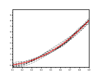
Figure 1: Plots of $J_{0,1}$ and of $10$ adaptive estimations when $H=0.6$ ($\overline{\widehat{m}}=5.4$).

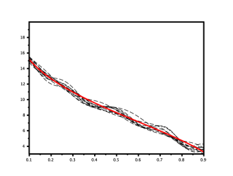
Figure 2: Plots of $J_{0,2}$ and of $10$ adaptive estimations when $H=0.6$ ($\overline{\widehat{m}}=11.2$).

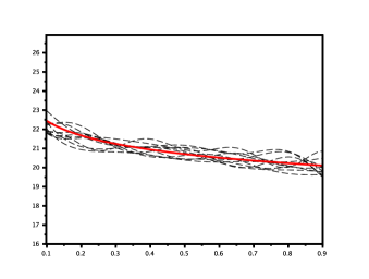
Figure 3: Plots of $J_{0,3}$ and of $10$ adaptive estimations when $H=0.6$ ($\overline{\widehat{m}}=8.2$).

On average, the MISE of our adaptive estimator is lower for the three examples of functions $J_{0}$ when $H=0.6$ than when $H=0.9$. The standard deviation of the MISE of $\widehat{J}_{\widehat{m},N,n}$ is also higher when $H=0.9$. For $H=0.6$, our estimation method seems stable in the sense that the standard deviation of the MISE of our adaptive estimator is almost the same for the three examples of functions $J_{0}$. This can be observed on Figures 1, 2 and 3. For $H=0.9$, our estimation method seems less stable. Finally, for both $H=0.6$ and $H=0.9$, on average, the MISE of $\widehat{J}_{\widehat{m},N,n}$ is higher for $J_{0,2}$ than for $J_{0,1}$ and $J_{0,3}$. This is probably related to the fact that $J_{0,2}(t)$ goes faster to infinity when $t\rightarrow 0^{+}$ than $J_{0,3}(t)$, and of course than $J_{0,1}(t)$ which doesn’t go. In conclusion, the numerical experiments show that when $Z$ is driven by the Molchan martingale, our estimation method of $J_{0}$ is satisfactory on several types of functions, but the MISE of $\widehat{J}_{\widehat{m},N,n}$ seems to increase when $H$ is near to $1$.

5.2 Experiments in the non-autonomous Black-Scholes model

Some numerical experiments on our estimation method of $b_{0}$ in the non-autonomous Black-Scholes model (15) are presented in this subsection on simulated prices datasets with $S_{0}=10$, $\sigma\in\{0.2,1\}$ and $b_{0}=\mathfrak{b}$, where

$$\mathfrak{b}(t):=\sin(2\pi t)+\cos(2\pi t)\textrm{$;$ }\forall t\in\mathbb{R}_{+}.$$

The function $\mathfrak{b}$ is estimated on $[0,1]$ (1 day), but the prices process $S$ of the asset is simulated on $N=100$ days via the non-autonomous Black-Scholes model (15). As explained at Subsection 4.3, here, $Z^{1},\dots,Z^{N}$ are obtained via (16) from the i.i.d. processes $S^{1},\dots,S^{N}$ defined by

$$S_{t}^{i}:=S_{i-1+t}\textrm{$;$ }\forall t\in[0,1].$$

Our adaptive estimator is computed for $S_{0}=10$ and $\sigma\in\{0.2,1\}$ on the paths of $Z^{1},\dots,Z^{N}$ obtained from one path of the prices process observed along the dissection $\{100l/n\textrm{$;$ }l=0,\dots,n\}$ of $[0,100]$ with $n=N^{2}=10000$, when $(\varphi_{1},\dots,\varphi_{m})$ is the $m$-dimensional trigonometric basis for every $m\in\{2,\dots,12\}$. Note that for $\sigma=0.2$, the path of $S$ is plotted on Figure 4, and the associated paths of $Z^{1},\dots,Z^{N}$ are plotted on Figure 5.

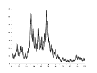
Figure 4: Plot of one path of the non-autonomous Black-Scholes model with $\sigma=0.2$.

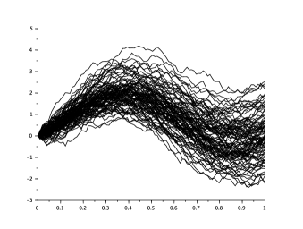
Figure 5: Plots of the paths of $Z^{1},\dots,Z^{N}$ associated to the path of $S$ at Figure 4.

This experiment is repeated 100 times, and the means and the standard deviations of the MISE of $\widehat{b}_{\widehat{m},N,n}:=\sigma\widehat{J}_{\widehat{m},N,n}$ are stored in Table 2.

$\sigma$	$0.2$	$1$
Mean MISE	0.002	0.042
StD MISE	0.002	0.046

Table 2: Means and StD of the MISE of $\widehat{b}_{\widehat{m},N,n}$ (100 repetitions).

Moreover, for $\sigma=0.2$ and $\sigma=1$, 10 estimations (dashed black curves) of $b_{0}=\mathfrak{b}$ (red curve) are respectively plotted on Figures 6 and 7.

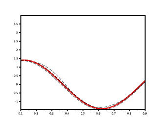
Figure 6: Plots of $\mathfrak{b}$ and of $10$ adaptive estimations when $\sigma=0.2$ ($\overline{\widehat{m}}=3.3$).

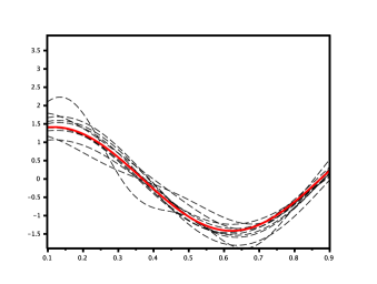
Figure 7: Plots of $\mathfrak{b}$ and of $10$ adaptive estimations when $\sigma=1$ ($\overline{\widehat{m}}=3.5$).

On average, the MISE of our adaptive estimator is obviously lower when $\sigma=0.2$ than when $\sigma=1$, but it remains globally small. Assume now that $\sigma$ is unknown as in practice. Then, it is estimated directly on the observed path of $S$ on $[0,100]$ by

$$\widehat{\sigma}_{N,n}:=\sqrt{\frac{1}{T_{N,n}}\sum_{l=0}^{n-1}[\log(S_{(l+1)N/n})-\log(S_{lN/n})]^{2}}\quad{\rm with}\quad T_{N,n}=nN$$

as usual (see Genon-Catalot GC12 , Subsubsection 3.2.2). The same experiment is then repeated on

$$\widetilde{b}_{\widehat{m},N,n}:=\widehat{\sigma}_{N,n}\widehat{J}_{\widehat{m},N,n}$$

instead of $\widehat{b}_{\widehat{m},N,n}$. The means and the standard deviations of the MISE of $\widetilde{b}_{\widehat{m},N,n}$ remain of same order (see Table 3).

$\sigma$ (mean $\widehat{\sigma}_{N,n}$)	$0.2$ (0.223)	$1$ (1.005)
Mean MISE	0.001	0.042
StD MISE	0.001	0.038

Table 3: Means and StD of the MISE of $\widetilde{b}_{\widehat{m},N,n}$ (100 repetitions).

Acknowledgments. Thank you to Fabienne Comte for her valuable comments on this paper.

References

- (1) Y. Baraud, F. Comte and G. Viennet. Model Selection for (Auto-)Regression with Dependent Data. ESAIM:PS 5, 33-49, 2001.
- (2) A. Cohen, M.A. Leviatan and D. Leviatan. On the Stability and Accuracy of Least Squares Approximations. Found. Comput. Math. 13, 819-834, 2013.
- (3) F. Comte, L. Coutin and E. Renault. Affine Fractional Stochastic Volatility Models. Annals of Finance 8, 337-378, 2012.
- (4) F. Comte and V. Genon-Catalot. Regression Function Estimation on Non Compact Support as a Partly Inverse Problem. The Annals of the Institute of Statistical Mathematics 72, 4, 1023-1054, 2020.
- (5) F. Comte and V. Genon-Catalot. Nonparametric Drift Estimation for i.i.d. Paths of Stochastic Differential Equations. The Annals of Statistics 48, 6, 3336-3365, 2020.
- (6) F. Comte and V. Genon-Catalot. Drift Estimation on Non Compact Support for Diffusion Models. Stoch. Proc. Appl. 134, 174-207, 2021.
- (7) F. Comte, V. Genon-Catalot and Y. Rozenholc. Penalized Nonparametric Mean Square Estimation of the Coefficients of Diffusion Processes. Bernoulli 12, 2, 514-543, 2007.
- (8) F. Comte and N. Marie. Nonparametric Estimation for I.I.D. Paths of Fractional SDE. Statistical Inference for Stochastic Processes 24, 3, 669-705, 2021.
- (9) A. Dalalyan. Sharp Adaptive Estimation of the Trend Coefficient for Ergodic Diffusion. The Annals of Statistics 33, 6, 2507-2528, 2005.
- (10) M. Delattre, V. Genon-Catalot and C. Larédo. Parametric Inference for Discrete Observations of Diffusion Processes with Mixed Effects. Stoch. Proc. Appl. 128, 1929-1957, 2018.
- (11) M. Delattre and M. Lavielle. Coupling the SAEM Algorithm and the Extended Kalman Filter for Maximum Likelihood Estimation in Mixed-Effects Diffusion Models. Stat. Interface 6, 519-532, 2013.
- (12) L. Della Maestra and M. Hoffmann. Nonparametric Estimation for Interacting Particle Systems: McKean-Vlasov Models. To appear in Probability Theory and Related Fields, 2021.
- (13) C. Denis, C. Dion and M. Martinez. A Ridge Estimator of the Drift from Discrete Repeated Observations of the Solutions of a Stochastic Differential Equation. To appear in Bernoulli, 2021.
- (14) R.A. DeVore and G.G. Lorentz. Constructive Approximation. Springer, 1993.
- (15) S. Ditlevsen and A. De Gaetano. Mixed Effects in Stochastic Differential Equation Models. REVSTAT 3, 137-153, 2005.
- (16) V. Genon-Catalot. Cours de statistique des diffusions. MSc. lecture notes, université Paris Cité, 2012.
- (17) M. Hoffmann. Adaptive Estimation in Diffusion Processes. Stoch. Proc. Appl. 79, 135-163, 1999.
- (18) M.L. Kleptsyna and A. Le Breton. Some Explicit Statistical Results About Elementary Fractional Type Models. Nonlinear Analysis 47, 4783-4794, 2001.
- (19) K. Kubilius, Y. Mishura and K. Ralchenko. Parameter Estimation in Fractional Diffusion Models. Springer, 2017.
- (20) Y. Kutoyants. Statistical Inference for Ergodic Diffusion Processes. Springer, 2004.
- (21) G. Lorentz, M. von Golitschek and Y. Makokov. Constructive Approximation, Advanced Problems. Springer, 1996.
- (22) N. Marie and A. Rosier. Nadaraya-Watson Estimator for I.I.D. Paths of Diffusion Processes. To appear in Scandinavian Journal of Statistics, 2022.
- (23) I. Norros, E. Valkeila and J. Virtamo. An Elementary Approach to a Girsanov Formula and Other Analytical Results on Fractional Brownian Motions. Bernoulli 5, 4, 571-587, 1999.
- (24) U. Picchini, A. De Gaetano and S. Ditlevsen. Stochastic Differential Mixed-Effects Models. Scand. J. Stat. 37, 67-90, 2010.
- (25) D. Revuz and M. Yor. Continuous Martingales and Brownian Motion. Springer, 1999.
- (26) S.G. Samko, A.A. Kilbas and O.I. Marichev. Fractional Integrals and Derivatives: Theory and Applications. CRC Press, 1993.
- (27) J.B. Wiggins. Option Values Under Stochastic Volatility. Theory and Empirical Estimates. Journal of Financial Economics 19, 351-372, 1987.