Training Integrable Parameterizations of Deep Neural Networks in the Infinite-Width Limit

Karl Hajjar Corresponding author: hajjarkarl@gmail.com Laboratoire de Mathématiques d’Orsay
Université Paris-Saclay
91405 Orsay, France
Lénaïc Chizat Institut de Mathématiques
École Polytechnique Fédérale de Lausanne
Lausanne, Switzerland
Christophe Giraud Laboratoire de Mathématiques d’Orsay
Université Paris-Saclay
91405 Orsay, France
Abstract

To theoretically understand the behavior of trained deep neural networks, it is necessary to study the dynamics induced by gradient methods from a random initialization. However, the nonlinear and compositional structure of these models make these dynamics difficult to analyze. To overcome these challenges, large-width asymptotics have recently emerged as a fruitful viewpoint and led to practical insights on real-world deep networks. For two-layer neural networks, it has been understood via these asymptotics that the nature of the trained model radically changes depending on the scale of the initial random weights, ranging from a kernel regime (for large initial variance) to a feature learning regime (for small initial variance). For deeper networks more regimes are possible, and in this paper we study in detail a specific choice of “small” initialization corresponding to “mean-field” limits of neural networks, which we call integrable parameterizations (IPs).

First, we show that under standard i.i.d. zero-mean initialization, integrable parameterizations of neural networks with more than four layers start at a stationary point in the infinite-width limit and no learning occurs. We then propose various methods to avoid this trivial behavior and analyze in detail the resulting dynamics. In particular, one of these methods consists in using large initial learning rates, and we show that it is equivalent to a modification of the recently proposed maximal update parameterization μ𝜇\muP. We confirm our results with numerical experiments on image classification tasks, which additionally show a strong difference in behavior between various choices of activation functions that is not yet captured by theory.

1 Introduction

While artificial neural networks routinely achieve state-of-the art performance in various real-world machine learning tasks, it is still a theoretical challenge to understand why and under which conditions they perform so well. The training algorithm—typically a variant of stochastic gradient descent (SGD) with random initialization—plays a central role in this performance but is difficult to analyze for general neural network architectures, because of their highly non-linear and compositional structure. Large-width asymptotics, which have previously been considered for other purposes (Neal, 1995; Bengio et al., 2006), have recently been proposed to overcome some of these difficulties and have brought numerous insights on the training behavior of neural networks (Nitanda and Suzuki, 2017; Mei et al., 2018; Jacot et al., 2018; Rotskoff and Vanden-Eijnden, 2018; Chizat and Bach, 2018; Sirignano and Spiliopoulos, 2020).

One of these insights is that the magnitude of the random weights at initialization has a dramatic impact on the learning behavior of neural networks (Chizat et al., 2019). For two-layer networks and with suitable learning rates, initializing the output layer weights with a standard deviation of 1/m1𝑚1/m, where m𝑚m is the width of the network, leads to feature learning when m𝑚m is large, while the same network initialized with a standard deviation of 1/m1𝑚1/\sqrt{m} leads to the Neural Tangent Kernel (NTK) regime, a.k.a. lazy regime, where the network simply learns a linear predictor on top of fixed features. This observation suggests that parameterizations—that is, the choice of the scaling factors, with the width m𝑚m, of the initial magnitude and of the learning rates of each layer of a neural network—are of fundamental importance in the theory of neural networks. While standard deep learning packages offer various choices of scale at initialization (Glorot and Bengio, 2010; He et al., 2015), those have been designed with the sole criterion in mind to have a non-vanishing first forward and backward passes for arbitrary depths. Theory now offers the tools to explore a larger space of parameterizations and study their dynamics beyond the first forward and backward passes in the infinite-width limit.

With more than two layers, the categorization of parameterizations is more subtle and there are disparate lines of work. On the one hand, some parameterizations still lead to the kernel regime, which is subject to an intense research activity (e.g., Jacot et al., 2018, 2019; Allen-Zhu et al., 2019; Du et al., 2019; Arora et al., 2019; Geiger et al., 2020a, c; Yang, 2020a). Since this regime reduces to learning a linear predictor on top of fixed features in the large width limit, this parameterization is of limited relevance to understand representation learning in networks used in practice (although it should be noted that non-asymptotic analyses reveal interesting effects, e.g., Hanin and Nica, 2019). On the other hand, there is a growing literature around parameterizations where weights are initialized with a standard deviation of 1/m1𝑚1/m (except for the first layer). These are often called “mean-field” models but we prefer to call them integrable parameterizations (IPs) in this work111For deep neural networks, it is somewhat arbitrary to associate the term mean-field with a specific choice of scaling so we believe that this term lacks precision when it comes to discussing various parameterizations., in reference to the fact that sums of m𝑚m terms with standard deviation of order of 1/m1𝑚1/m are absolutely convergent. There already exists mathematical tools to describe the evolution of the parameters of IPs in the infinite-width limit but they are not fully satisfactory to understand the properties of the learned function in the standard setting used in practice (see review in Section 1.2).

Going beyond the dichotomy between the scales 1/m1𝑚1/m and 1/m1𝑚1/\sqrt{m}, Yang and Hu (2021) have exhibited, using a technique called the Tensor Program (Yang, 2019, 2020a, 2020b), a general categorization of parameterizations, in particular between those which allow feature learning and those which do not. As a result from their analysis, they singled out a maximal update parameterization μ𝜇\muP where, as for the NTK parameterization, the intermediate layers’ weights are initialized with a standard deviation of 1/m1𝑚1/\sqrt{m}, but the last layer weights are initialized with a standard deviation of 1/m1𝑚1/m: they show that with appropriate learning rates, this leads to maximal feature learning (in a certain sense). This parameterization had been previously considered in (Geiger et al., 2020b) where the authors study empirically the effect of the scale (Chizat et al., 2019) on learning.

In (Yang and Hu, 2021), IPs have been excluded from the analysis on the basis that they are trivial: if one follows the usual training procedure—which we refer to as Naive-IP—the network starts on a stationary point in the infinite-width limit and the learned function remains at its initial value.

1.1 Contributions

Our goal is to draw connections between the various lines of research discussed above, and to improve our understanding of integrable parameterizations: when and why are they trivial? How can we avoid triviality and actually learn features? What are the salient properties of the resulting networks in the infinite-width limit? To answer these questions rigorously, we leverage the Tensor Program technique developed in (Yang, 2019, 2020a, 2020b; Yang and Hu, 2021). Specifically, our contributions are the following:

  • We first show in Theorem 3.1 that with learning rates constant in time, the functions learned using SGD for integrable parameterizations of neural networks with four layers or more either remain at their value at initialization or explode in the infinite-width limit when the weights are initialized using the standard zero-mean i.i.d. schemes used in practice.

  • We show in Theorem 4.1 that using large learning rates, which grow as a power of m𝑚m, for the first gradient step—and that step only—allows SGD to escape the initial stationary point for integrable parameterizations and to initiate a non-trivial learning phase. In fact, we prove in Theorem 4.2 that the resulting dynamic is equivalent to a modification of the dynamic of μ𝜇\muP  where, after the first gradient step, one subtracts the initial weights from the learned weights of the intermediate layers.

  • We study two alternative ways to escape the initial stationary point for integrable parameterizations and analyze the corresponding dynamics. Removing the scale factor in 1/m1𝑚1/m on the bias terms allows to escape the initial stationary point when using moderately large initial learning rates. A drawback of the resulting dynamics is that its updates only depend weakly on the input data (see Theorem 5.2). On the other hand, using a non-centered law also allows to escape the initial stationary point for i.i.d. initializations without having to use large learning rates, but the dynamics become degenerate as the updates of the entries of the weight matrix in a given layer are all equal to the same fixed quantity in the infinite-width limit (see Theorem 5.1). We investigate numerically the performance of those two models and show that the aforementioned behaviors are detrimental to learning.

The code to reproduce the results of the numerical experiments can be found at:
https://github.com/karl-hajjar/wide-networks.

1.2 Related Work

While the study of infinitely wide neural networks has a long history (Barron, 1993; Neal, 1995, 1996; Kurková and Sanguineti, 2001; Mhaskar, 2004; Bengio et al., 2006; Bach, 2017), it is only recently that their training dynamics have been investigated. Two-layer neural networks with IP enjoy some global convergence properties (Chizat and Bach, 2018) and favorable guarantees in terms of generalization (Bach, 2017; Chizat and Bach, 2020). Going beyond two layers, Nguyen and Pham (2020) and Pham and Nguyen (2020) study the infinite-width limit of IPs and also prove global convergence results for networks with three layers or more. However, those results hold for standard zero-mean i.i.d. initialization schemes only for networks with two or three layers (which is consistent with the results of Section 3.1): for deeper networks they require non-standard (correlated) initializations.

Several other works describe the infinite-width limit of multi-layer IPs: Araújo et al. (2019) characterize the infinite-width dynamics via a model of McKean-Vlasov type, for which they prove existence and uniqueness of solutions, and  Sirignano and Spiliopoulos (2021) prove a global convergence result for three-layer networks. They take the number of units in each layer to infinity sequentially and describe the dynamics of the limit as a system of differential equations over the weights/parameters. On the other hand, Fang et al. (2020) take the infinite-width limit for all layers at once (as in Araújo et al., 2019; Nguyen and Pham, 2020; Pham and Nguyen, 2020) and describe the resulting dynamics as an ODE over functions of the features (pre-activations) of the network. It is interesting to note that Araújo et al. (2019); Sirignano and Spiliopoulos (2021); Pham and Nguyen (2020) all discuss the difficulties associated with describing the dynamics of the infinite-width of IPs with more than three layers. As noted in (Araújo et al., 2019), and appropriately addressed by Nguyen and Pham (2020); Fang et al. (2020); Sirignano and Spiliopoulos (2021), there is a separation of time scales as soon as there are two hidden layers or more, where the gradients of the intermediate layers appear to scale as m2superscript𝑚2m^{-2} whereas the gradients of the input and output layers appear to scale as m1superscript𝑚1m^{-1}, requiring separate learning rate values which can make the analysis of the infinite-width limit more difficult.

In a separate line of work, Yang and Hu (2021) provide with the Tensor Program a theoretical tool to describe the infinite-width limit of different parameterizations of neural networks and categorize them between feature learning and kernel-like behavior. However, IPs with three layers or more are left out of this categorization. Using the same tools, we show that IPs with more than four layers are indeed trivial at any time step if the initial learning rates are not appropriately scaled with m𝑚m under standard zero-mean i.i.d. initializations. This closes the gap with (Nguyen and Pham, 2020) which proves global convergence results for IPs with two or three layers initialized using those standard schemes. We also demonstrate in Section 4 how scaling the initial learning rates appropriately allows to properly train an IP—inducing a feature learning regime as defined in (Yang and Hu, 2021)—and connect the resulting model with a version of the maximal update parameterization μ𝜇\muP (Yang and Hu, 2021) where the initial weights of the intermediate layers are replaced by zero in the first update.

The setting where non-centered i.i.d. initialization laws are used is covered in (Nguyen and Pham, 2020), where it is shown that a certain collapse phenomenon occurs, namely that the updates of the entries of the weight matrix in a given layer are all equal to the same deterministic quantity in the large-width limit. We obtain a similar result in Section 5.1 using different theoretical tools.

Tensor Program vs. other formalisms.

In contrast to prior literature on IPs, we do not use the description of the infinite-width limit as a composition of integral transforms. With the standard (centered i.i.d.) initializations considered in this paper, that description does not offer much insight about the limit beyond the fact that it starts on a stationary point. In order to escape this initial stationary point, we propose in this paper to amplify the random fluctuations around the limit using large initial learning rates. The strength of the Tensor Program formalism (Yang, 2019, 2020a, 2020b; Yang and Hu, 2021) is precisely that it is able to describe rigorously the magnitudes of these fluctuations and allows us to analyze the functions learned with various choices of learning rates. This formalism relies on techniques initiated in the statistical physics literature (Bayati and Montanari, 2011; Bolthausen, 2014) that use the Gaussian conditioning technique to describe the behavior of algorithms (such as message passing) involving random matrices and nonlinearities.

1.3 Organisation of the Paper and Notations

We define and analyze integrable parameterizations in Section 3 and show that they are trivial for common choices of learning rates. In Section 4, we describe how a specific scaling of the learning rates allows to escape the initial stationary point, and further investigate the connection between IPs with large initial learning rates and μ𝜇\muP. In Section 5, we present two alternative modifications of IPs to escape the initial stationary point and discuss the impact of each on the learning dynamics.

We defer all the rigorous proofs of our theoretical results to the Appendix, so as to make the core message of our work stand out more clearly, and keep the flow of the results structured and easy to follow. Among other things, this prevents us from diving too deep into the Tensor Program formalism and calculations (which can be somewhat tedious and abstruse) in the main part of our work. Most proofs require heavy inductions on the time step t𝑡t, and proving the induction step itself often involves inductions on l𝑙l in the forward pass (from l=1𝑙1l=1 to l=L𝑙𝐿l=L) and in the backward pass (from l=L𝑙𝐿l=L to l=1𝑙1l=1). Breaking down all these steps makes for a lengthy Appendix, but the ideas of the proof are relatively straightforward, only their proper formal writing is tedious.

Throughout the paper, for two integers p,q𝑝𝑞p,q, we denote by [p]delimited-[]𝑝[p] the set {1,,p}1𝑝\{1,\ldots,p\} and by [p,q]𝑝𝑞[p,q] the set {p,,q}𝑝𝑞\{p,\ldots,q\}. We write uvdirect-product𝑢𝑣u\odot v for the Hadamard (i.e., element-wise) product of two vectors u𝑢u and v𝑣v. We use Landau notations for comparing two real sequences (um)subscript𝑢𝑚(u_{m}) and (vm)subscript𝑣𝑚(v_{m}): we write um=O(vm)subscript𝑢𝑚𝑂subscript𝑣𝑚u_{m}=O(v_{m}) when there exists a constant C>0𝐶0C>0 such that |um|C|vm|subscript𝑢𝑚𝐶subscript𝑣𝑚|u_{m}|\leq C|v_{m}| for large enough m𝑚m, and um=Θ(vm)subscript𝑢𝑚Θsubscript𝑣𝑚u_{m}=\Theta(v_{m}) when we both have um=O(vm)subscript𝑢𝑚𝑂subscript𝑣𝑚u_{m}=O(v_{m}) and um=O(vm)subscript𝑢𝑚𝑂subscript𝑣𝑚u_{m}=O(v_{m}). We similarly use the O𝑂O (respectively ΘΘ\Theta) notation for two sequences of real-valued random variables (um)subscript𝑢𝑚(u_{m}) and (vm)subscript𝑣𝑚(v_{m}) when, almost surely, um=O(vm)subscript𝑢𝑚𝑂subscript𝑣𝑚u_{m}=O(v_{m}) (respectively um=Θ(vm)subscript𝑢𝑚Θsubscript𝑣𝑚u_{m}=\Theta(v_{m})).

2 General Setting

In this section, we introduce the general setting we consider for this work, as well as the corresponding notations. We also define precisely the notion of parameterization of a neural network and discuss examples of parameterizations commonly found in the literature.

2.1 Network and Data

Training data.

We consider a training dataset {(ξ(i),y(i))}i[n]subscriptsuperscript𝜉𝑖superscript𝑦𝑖𝑖delimited-[]𝑛\left\{(\xi^{(i)},y^{(i)})\right\}_{i\in[n]} containing n𝑛n (input, output) pairs with ξ(i)dsuperscript𝜉𝑖superscript𝑑\xi^{(i)}\in\mathbb{R}^{d} and y(i)superscript𝑦𝑖y^{(i)}\in\mathbb{R}. We will use ξ(i)superscript𝜉𝑖\xi^{(i)} or y(i)superscript𝑦𝑖y^{(i)} when we refer to the i𝑖i-th sample in the training dataset, but use ξtsubscript𝜉𝑡\xi_{t} and ytsubscript𝑦𝑡y_{t} to denote the sample(s) fed to train the network at time step t𝑡t, that is for the (t+1)𝑡1(t+1)-th step of optimization.

Width and depth.

Throughout this work, we consider a feed-forward fully connected neural network, with L𝐿L hidden layers and a common width m𝑚m. The total number of layers, i.e., weight matrices and bias vectors will thus be L+1𝐿1L+1, and most of our results are concerned with four or more layers, that is L3𝐿3L\geq 3, and in the limit m𝑚m\rightarrow\infty. The integer l[L+1]𝑙delimited-[]𝐿1l\in[L+1] will always be used to index the layers of a network, and we call the intermediate layers of a network the layers indexed by l[2,L]𝑙2𝐿l\in[2,L] (i.e., excluding input and output layers).

Activation function.

We assume that all the neurons in the network share the same activation function σ::𝜎\sigma:\mathbb{R}\to\mathbb{R}. The activation is always taken entry-wise and for any vector hmsuperscript𝑚h\in\mathbb{R}^{m}, we denote by σ(h)𝜎\sigma(h) the vector (σ(hp))p[m]msubscript𝜎subscript𝑝𝑝delimited-[]𝑚superscript𝑚(\sigma(h_{p}))_{p\in[m]}\in\mathbb{R}^{m}.

Weights and forward pass.

We denote by Wl(t)superscript𝑊𝑙𝑡W^{l}(t) and Bl(t)superscript𝐵𝑙𝑡B^{l}(t) respectively the weight matrix and bias vector of layer l𝑙l at time step t𝑡t (i.e., after t𝑡t steps of SGD), and thus have W1(t)m×dsuperscript𝑊1𝑡superscript𝑚𝑑W^{1}(t)\in\mathbb{R}^{m\times d}, Wl(t)m×msuperscript𝑊𝑙𝑡superscript𝑚𝑚W^{l}(t)\in\mathbb{R}^{m\times m} for l[2,L]𝑙2𝐿l\in[2,L] and WL+1(t)msuperscript𝑊𝐿1𝑡superscript𝑚W^{L+1}(t)\in\mathbb{R}^{m}. At any time step t𝑡t we denote by htl(ξ)subscriptsuperscript𝑙𝑡𝜉h^{l}_{t}(\xi) and xtl(ξ)subscriptsuperscript𝑥𝑙𝑡𝜉x^{l}_{t}(\xi) the pre-activations and activations respectively coming out of the l𝑙l-th layer when feeding input ξ𝜉\xi to the network (with the convention that xt0(ξ)=ξsubscriptsuperscript𝑥0𝑡𝜉𝜉x^{0}_{t}(\xi)=\xi). That is

htl(ξ):=Wl(t)xtl1(ξ)+Bl(t),assignsubscriptsuperscript𝑙𝑡𝜉superscript𝑊𝑙𝑡subscriptsuperscript𝑥𝑙1𝑡𝜉superscript𝐵𝑙𝑡\displaystyle h^{l}_{t}(\xi):=W^{l}(t)x^{l-1}_{t}(\xi)+B^{l}(t), and xtl(ξ):=σ(htl(ξ)),assignsubscriptsuperscript𝑥𝑙𝑡𝜉𝜎subscriptsuperscript𝑙𝑡𝜉\displaystyle x^{l}_{t}(\xi):=\sigma(h^{l}_{t}(\xi)), forl[1,L].for𝑙1𝐿\displaystyle\textrm{for}\ l\in[1,L]. (2.1)
Output.

We denote the output of the network by

ft(ξ)=f(θ(t);ξ):=(WL+1(t))xtL(ξ)+BL+1(t),subscript𝑓𝑡𝜉𝑓𝜃𝑡𝜉assignsuperscriptsuperscript𝑊𝐿1𝑡subscriptsuperscript𝑥𝐿𝑡𝜉superscript𝐵𝐿1𝑡f_{t}(\xi)=f(\theta(t);\xi):={(W^{L+1}(t))}^{\intercal}x^{L}_{t}(\xi)+B^{L+1}(t), (2.2)

where θ(t)𝜃𝑡\theta(t) denotes the set of all network parameters at time t𝑡t. We often drop the dependency of the forward pass on the input ξ𝜉\xi for brevity and simply use htl,xtlsubscriptsuperscript𝑙𝑡subscriptsuperscript𝑥𝑙𝑡h^{l}_{t},x^{l}_{t} instead of htl(ξ),xtl(ξ)subscriptsuperscript𝑙𝑡𝜉subscriptsuperscript𝑥𝑙𝑡𝜉h^{l}_{t}(\xi),x^{l}_{t}(\xi) as it should always be clear from the context which input is being fed to the network. Note that the weights and biases as well as all the (pre-)activations depend on the width m𝑚m of the network (through their dimensions) but we omit this dependency for clarity.

Loss.

We denote by \ell the loss function used to train the network, which is a function from 2superscript2\mathbb{R}^{2} to \mathbb{R}. The fit of a prediction y^^𝑦\widehat{y} is thus measured by (y,y^)𝑦^𝑦\ell(y,\widehat{y}) where y𝑦y is the desired output. In all this work, we make the following assumption on the loss function \ell, which is met by most common loss functions:

Assumption 1 (Smooth loss w.r.t second argument).

The loss \ell is differentiable with respect to its second argument and 2(y,)subscript2𝑦\partial_{2}\ell(y,\cdot) is a continuous function for any y𝑦y\in\mathbb{R}.

Assumption 1 is essentially here to guarantee that if the sequence (y^(m))msubscriptsuperscript^𝑦𝑚𝑚superscript(\widehat{y}^{(m)})_{m\in\mathbb{N}^{*}} converges almost surely to some y^()superscript^𝑦\widehat{y}^{(\infty)}, then 2(y,y^(m))subscript2𝑦superscript^𝑦𝑚\partial_{2}\ell(y,\widehat{y}^{(m)}) also converges almost surely to 2(y,y^())subscript2𝑦superscript^𝑦\partial_{2}\ell(y,\widehat{y}^{(\infty)}).

2.2 Parameterizations of Neural Networks

The fact that the magnitude of the initialization of the weights and of the scale pre-factor for the weights are key quantities that determine the learning regime achieved by neural networks—and more generally by differentiable models—was pointed out in (Chizat et al., 2019). In this paper, we are interested in the behavior of neural networks when their width m𝑚m goes to infinity, and we refer to as a parameterization of a neural network the choice of how (a) the pre-factor of the weights, (b) the variance at initialization and (c) the learning rates, evolve as a function of m𝑚m. This concept was called an abc-parameterization by  Yang and Hu (2021), because these dependencies are given by masuperscript𝑚𝑎m^{-a}, mbsuperscript𝑚𝑏m^{-b} and mcsuperscript𝑚𝑐m^{-c}.

As explained by these authors, one of those three choices is actually redundant, and one can do with only the choice of two among those three scales. We take the point view considering a parameterization as a choice of scale for the pre-factor of the weights (a) and a choice of scale for the learning rates (c) while the random weights are always initialized (b) with standard i.i.d. Gaussians 𝒩(0,1)𝒩01\mathcal{N}(0,1). We make this (arbitrary) choice as typically in the literature, different models of the infinite-width limit correspond to different choices of scales for the weights’ pre-factors, e.g., NTK corresponds to a pre-factor in 1/m1𝑚1/\sqrt{m} while “mean-field” models correspond to a choice of pre-factor in 1/m1𝑚1/m for the weights. We thus define below ac-parameterizations which are a slight variation of the abc-parameterizations introduced in (Yang and Hu, 2021).

Definition 2.1.

(ac-parameterization). An ac-parameterization of an L𝐿L-hidden layer fully-connected neural network is a choice of scalar exponents (a1,,aL+1)subscript𝑎1subscript𝑎𝐿1(a_{1},\ldots,a_{L+1}), and (c1,,cL+1)subscript𝑐1subscript𝑐𝐿1(c_{1},\ldots,c_{L+1}) such that for any layer l[L+1]𝑙delimited-[]𝐿1l\in[L+1],

  1. (i)

    the learnable weights (i.e., those over which we optimize) are initialized with independent standard Gaussian random variables wjql(0)𝒩(0,1)similar-tosubscriptsuperscript𝑤𝑙𝑗𝑞0𝒩01w^{l}_{jq}(0)\sim\mathcal{N}(0,1), i.i.d. over (l,j,q)𝑙𝑗𝑞(l,j,q), i.e., wl(0)=Ulsuperscript𝑤𝑙0superscript𝑈𝑙w^{l}(0)=U^{l} with (Ul)l[L+1]subscriptsuperscript𝑈𝑙𝑙delimited-[]𝐿1(U^{l})_{l\in[L+1]} independent random matrices with i.i.d. standard Gaussian entries,

  2. (ii)

    the learnable biases are initialized independently of the weights, with bjl(0)𝒩(0,1)similar-tosubscriptsuperscript𝑏𝑙𝑗0𝒩01b^{l}_{j}(0)\sim\mathcal{N}(0,1), i.i.d. over (l,j)𝑙𝑗(l,j), i.e., bl(0)=vlsuperscript𝑏𝑙0superscript𝑣𝑙b^{l}(0)=v^{l} with (vl)l[L+1]subscriptsuperscript𝑣𝑙𝑙delimited-[]𝐿1(v^{l})_{l\in[L+1]} independent standard Gaussian random vectors, independent of Ulsuperscript𝑈𝑙U^{l},

  3. (iii)

    the effective weights Wl(t)superscript𝑊𝑙𝑡W^{l}(t) used to compute the pre-activations at time t𝑡t are Wl(t)=malwl(t)superscript𝑊𝑙𝑡superscript𝑚subscript𝑎𝑙superscript𝑤𝑙𝑡W^{l}(t)=m^{-a_{l}}w^{l}(t), and the effective biases are Bl(t)=malbl(t)superscript𝐵𝑙𝑡superscript𝑚subscript𝑎𝑙superscript𝑏𝑙𝑡B^{l}(t)=m^{-a_{l}}b^{l}(t), so that the pre-activations are

    htl=Wl(t)xtl1+Bl(t)=mal(wl(t)σ(htl1)+bl(t)),l[1,L],formulae-sequencesubscriptsuperscript𝑙𝑡superscript𝑊𝑙𝑡subscriptsuperscript𝑥𝑙1𝑡superscript𝐵𝑙𝑡superscript𝑚subscript𝑎𝑙superscript𝑤𝑙𝑡𝜎subscriptsuperscript𝑙1𝑡superscript𝑏𝑙𝑡𝑙1𝐿\displaystyle h^{l}_{t}=W^{l}(t)x^{l-1}_{t}+B^{l}(t)=m^{-a_{l}}\left(w^{l}(t)\sigma(h^{l-1}_{t})+b^{l}(t)\right),\quad l\in[1,L],

    and the output is

    f(θ(t);ξ)=maL+1(wL+1(t)Tσ(htL(ξ))+bL+1(t)),𝑓𝜃𝑡𝜉superscript𝑚subscript𝑎𝐿1superscript𝑤𝐿1superscript𝑡𝑇𝜎subscriptsuperscript𝐿𝑡𝜉superscript𝑏𝐿1𝑡f(\theta(t);\xi)=m^{-a_{L+1}}\left(w^{L+1}(t)^{T}\sigma(h^{L}_{t}(\xi))+b^{L+1}(t)\right),
  4. (iv)

    the (t+1)𝑡1(t+1)-th update of learnable weights and biases is given by the update rules

    Δwl(t+1)Δsuperscript𝑤𝑙𝑡1\displaystyle\Delta w^{l}(t+1) :=wl(t+1)wl(t)=ηmclwl(yt,f(θ(t);ξt)),assignabsentsuperscript𝑤𝑙𝑡1superscript𝑤𝑙𝑡𝜂superscript𝑚subscript𝑐𝑙subscriptsuperscript𝑤𝑙subscript𝑦𝑡𝑓𝜃𝑡subscript𝜉𝑡\displaystyle:=w^{l}(t+1)-w^{l}(t)=-\eta m^{-c_{l}}\nabla_{w^{l}}\ell\left(y_{t},f(\theta(t);\xi_{t})\right),
    Δbl(t+1)Δsuperscript𝑏𝑙𝑡1\displaystyle\Delta b^{l}(t+1) :=bl(t+1)bl(t)=ηmclbl(yt,f(θ(t);ξt)),assignabsentsuperscript𝑏𝑙𝑡1superscript𝑏𝑙𝑡𝜂superscript𝑚subscript𝑐𝑙subscriptsuperscript𝑏𝑙subscript𝑦𝑡𝑓𝜃𝑡subscript𝜉𝑡\displaystyle:=b^{l}(t+1)-b^{l}(t)=-\eta m^{-c_{l}}\nabla_{b^{l}}\ell\left(y_{t},f(\theta(t);\xi_{t})\right),

    where θ(t)={(w1(t),b1(t)),,(wL+1(t),bL+1(t))}𝜃𝑡superscript𝑤1𝑡superscript𝑏1𝑡superscript𝑤𝐿1𝑡superscript𝑏𝐿1𝑡\theta(t)=\left\{(w^{1}(t),b^{1}(t)),\ldots,(w^{L+1}(t),b^{L+1}(t))\right\} is the full set of all network parameters, (ξt,yt)subscript𝜉𝑡subscript𝑦𝑡(\xi_{t},y_{t}) represent the input(s) and target(s) to the network at step t𝑡t and η+𝜂superscriptsubscript\eta\in\mathbb{R}_{+}^{*} is the scalar part of the learning rate which does not depend on m𝑚m and which we call the base learning rate. We denote by ηl:=ηmclassignsubscript𝜂𝑙𝜂superscript𝑚subscript𝑐𝑙\eta_{l}:=\eta m^{-c_{l}} the full learning rate for layer l𝑙l.

Remark 2.1.
  1. 1.

    Compared to the definition of (Yang and Hu, 2021), we allow for different values of clsubscript𝑐𝑙c_{l} at different layers and remove the redundant initialization scale (the b in abc-parameterizations). Any abc-parameterization with constant c𝑐c for all layers (as presented in Yang and Hu, 2021) can be recovered (same effective weights and biases at any time step) with an ac-parameterization with individual learning rates at each layer via the re-parameterization alal+blsubscript𝑎𝑙subscript𝑎𝑙subscript𝑏𝑙a_{l}\leftarrow a_{l}+b_{l}, bl0subscript𝑏𝑙0b_{l}\leftarrow 0, cl:=c2blassignsubscript𝑐𝑙𝑐2subscript𝑏𝑙c_{l}:=c-2b_{l}.

  2. 2.

    As we study the infinite-width limit m𝑚m\rightarrow\infty, we need to consider an infinite number of random weights at initialization. To this end, we consider for any l[2,L]𝑙2𝐿l\in[2,L], two infinite lists of i.i.d. standard Gaussian variables, independent of each other: (Ujql)j,qsubscriptsubscriptsuperscript𝑈𝑙𝑗𝑞𝑗𝑞superscript(U^{l}_{jq})_{j,q\in\mathbb{N}^{*}} and (vjl)psubscriptsubscriptsuperscript𝑣𝑙𝑗𝑝superscript(v^{l}_{j})_{p\in\mathbb{N}^{*}}, and often simply call, by an abuse of notations, Ul=(Ujql)1j,qmsuperscript𝑈𝑙subscriptsubscriptsuperscript𝑈𝑙𝑗𝑞formulae-sequence1𝑗𝑞𝑚U^{l}=(U^{l}_{jq})_{1\leq j,q\leq m} for the corresponding matrix at width m𝑚m and vl=(vjl)1jmsuperscript𝑣𝑙subscriptsubscriptsuperscript𝑣𝑙𝑗1𝑗𝑚v^{l}=(v^{l}_{j})_{1\leq j\leq m} the corresponding bias vector at width m𝑚m. We proceed similarly at initialization for the input weights U1superscript𝑈1U^{1} and the output vector UL+1superscript𝑈𝐿1U^{L+1}.

  3. 3.

    The (t+1)𝑡1(t+1)-th update of the effective weights is given by ΔWl(t+1):=Wl(t+1)Wl(t)=ηm(2al+cl)wl(yt,f(θ(t);ξt))assignΔsuperscript𝑊𝑙𝑡1superscript𝑊𝑙𝑡1superscript𝑊𝑙𝑡𝜂superscript𝑚2subscript𝑎𝑙subscript𝑐𝑙subscriptsuperscript𝑤𝑙subscript𝑦𝑡𝑓𝜃𝑡subscript𝜉𝑡\Delta W^{l}(t+1):=W^{l}(t+1)-W^{l}(t)=-\eta m^{-(2a_{l}+c_{l})}\nabla_{w^{l}}\ell(y_{t},f(\theta(t);\xi_{t})), and the update of the effective biases by ΔBl(t+1):=Bl(t+1)Bl(t)=ηm(2al+cl)bl(yt,f(θ(t);ξt))assignΔsuperscript𝐵𝑙𝑡1superscript𝐵𝑙𝑡1superscript𝐵𝑙𝑡𝜂superscript𝑚2subscript𝑎𝑙subscript𝑐𝑙subscriptsuperscript𝑏𝑙subscript𝑦𝑡𝑓𝜃𝑡subscript𝜉𝑡\Delta B^{l}(t+1):=B^{l}(t+1)-B^{l}(t)=-\eta m^{-(2a_{l}+c_{l})}\nabla_{b^{l}}\ell(y_{t},f(\theta(t);\xi_{t}))

Examples of ac-parameterizations:
NTK parameterization.

For the NTK parametrization (Jacot et al., 2018) the scaling is a1=0subscript𝑎10a_{1}=0 for the input layer, and al=1/2subscript𝑎𝑙12a_{l}=1/2 for all the other layers l[2,L+1]𝑙2𝐿1l\in[2,L+1]. The scaling of the learning rates is cl=0subscript𝑐𝑙0c_{l}=0 for all layers. Neural networks in the NTK parametrization have been shown to behave as kernel methods in the infinite-width limit (Jacot et al., 2018; Yang, 2020a) and there is no feature learning in that limit.

μ𝜇\muP.

To avoid the lazy training phenomenon arising in the NTK parameterization, Yang and Hu (2021) propose to adjust the scale of the output layer by setting aL+1=1subscript𝑎𝐿11a_{L+1}=1, while keeping a1=0subscript𝑎10a_{1}=0 and al=1/2subscript𝑎𝑙12a_{l}=1/2 for the intermediate layers l[2,L]𝑙2𝐿l\in[2,L]. The learning rates are appropriately adjusted: cl=1subscript𝑐𝑙1c_{l}=-1 for any layer l𝑙l. With this parameterization, Yang and Hu (2021) show that feature learning (see Definition B.1 in Appendix B.3 for a precise statement) occurs at every layer.

Integrable Parameterizations (IPs).

The limits investigated in Araújo et al. (2019); Sirignano and Spiliopoulos (2021); Pham and Nguyen (2020); Weinan and Wojtowytsch (2020) are associated to a scale multiplier in 1/m1𝑚1/m for all layers except the first one. This corresponds to the choice a1=0subscript𝑎10a_{1}=0 and al=1subscript𝑎𝑙1a_{l}=1 for l[2,L+1]𝑙2𝐿1l\in[2,L+1]. We choose the adjective “integrable” in reference to the absolute convergence of sums of the form (1/m)qxq1𝑚subscript𝑞subscript𝑥𝑞(1/m)\sum_{q}x_{q} for i.i.d. random variables with finite expectation. Integrable parameterizations really refer to a class of ac-parameterizations, because various choices for the learning rate exponents clsubscript𝑐𝑙c_{l} are admissible.

Naive-IP.

In the mean-field literature, integrable parameterizations often come with the standard learning rates corresponding to c1=cL+1=1subscript𝑐1subscript𝑐𝐿11c_{1}=c_{L+1}=-1 for the input/output layers and cl=2subscript𝑐𝑙2c_{l}=-2 for the intermediate layers l[2,L]𝑙2𝐿l\in[2,L], see e.g., (Araújo et al., 2019, Remark 3.4), (Fang et al., 2020, Algorithm 1), (Weinan and Wojtowytsch, 2020, Lemma 5.1), and (Sirignano and Spiliopoulos, 2021, Equation 4.3). Mean-field models with these learning rates are the natural counterparts of the infinite-width limits where sums are replaced by integrals, and we call the integrable parameterization with this specific choice of learning rates the Naive Integrable Parameterization.

When L=1𝐿1L=1, μ𝜇\muP and the Naive-IP coincide. For deeper networks, in the setting of abc-parameterizations described in (Yang and Hu, 2021), μ𝜇\muP and Naive-IP correspond to the same parameterization (same values for a and c) except that the weights of the intermediate layers are initialized with a standard deviation of 1/m1𝑚1/m for Naive-IP instead of 1/m1𝑚1/\sqrt{m} for μ𝜇\muP, that is they are downscaled by 1/m1𝑚1/\sqrt{m} compared to μ𝜇\muP. In Section 4.2, we show that there is also a close relationship between μ𝜇\muP and IP with large initial learning rates.

We give below an intuitive explanation for the choice c1=cL+1=1subscript𝑐1subscript𝑐𝐿11c_{1}=c_{L+1}=-1 and cl=2subscript𝑐𝑙2c_{l}=-2 for l[2,L]𝑙2𝐿l\in[2,L] for the scaling of the learning rates in Naive-IP. For l[2,L]𝑙2𝐿l\in[2,L], we have htl=m1(wl(t)xtl1+bl(t))subscriptsuperscript𝑙𝑡superscript𝑚1superscript𝑤𝑙𝑡subscriptsuperscript𝑥𝑙1𝑡superscript𝑏𝑙𝑡h^{l}_{t}=m^{-1}(w^{l}(t)x^{l-1}_{t}+b^{l}(t)), so that wlft(ξt)=m1(hlft(ξt))(xtl1)subscriptsuperscript𝑤𝑙subscript𝑓𝑡subscript𝜉𝑡superscript𝑚1subscriptsuperscript𝑙subscript𝑓𝑡subscript𝜉𝑡superscriptsubscriptsuperscript𝑥𝑙1𝑡\nabla_{w^{l}}f_{t}(\xi_{t})=m^{-1}(\nabla_{h^{l}}f_{t}(\xi_{t})){(x^{l-1}_{t})}^{\intercal}. In addition wL+1ft(ξt)=xtL/msubscriptsuperscript𝑤𝐿1subscript𝑓𝑡subscript𝜉𝑡subscriptsuperscript𝑥𝐿𝑡𝑚\nabla_{w^{L+1}}f_{t}(\xi_{t})=x^{L}_{t}/m and w1ft(ξt)=(h1ft(ξt))(ξt)subscriptsuperscript𝑤1subscript𝑓𝑡subscript𝜉𝑡subscriptsuperscript1subscript𝑓𝑡subscript𝜉𝑡superscriptsubscript𝜉𝑡\nabla_{w^{1}}f_{t}(\xi_{t})=(\nabla_{h^{1}}f_{t}(\xi_{t})){(\xi_{t})}^{\intercal}. So for one step of SGD:

ΔW1(t+1)ξt+1Δsuperscript𝑊1𝑡1subscript𝜉𝑡1\displaystyle\Delta W^{1}(t+1)\xi_{t+1} =η2(yt,ft(ξt))(ξtξt+1)m(1+c1)(mh1ft(ξt)).absent𝜂subscript2subscript𝑦𝑡subscript𝑓𝑡subscript𝜉𝑡superscriptsubscript𝜉𝑡subscript𝜉𝑡1superscript𝑚1subscript𝑐1𝑚subscriptsuperscript1subscript𝑓𝑡subscript𝜉𝑡\displaystyle=-\eta\partial_{2}\ell(y_{t},f_{t}(\xi_{t}))({\xi_{t}}^{\intercal}\xi_{t+1})m^{-(1+c_{1})}(m\nabla_{h^{1}}f_{t}(\xi_{t})). (2.3)
ΔWl(t+1)xt+1l1Δsuperscript𝑊𝑙𝑡1subscriptsuperscript𝑥𝑙1𝑡1\displaystyle\Delta W^{l}(t+1)x^{l-1}_{t+1} =η2(yt,ft(ξt))m(2+cl)(xtl1)xt+1l1m(mhlft(ξt)),forl[2,L]formulae-sequenceabsent𝜂subscript2subscript𝑦𝑡subscript𝑓𝑡subscript𝜉𝑡superscript𝑚2subscript𝑐𝑙superscriptsubscriptsuperscript𝑥𝑙1𝑡subscriptsuperscript𝑥𝑙1𝑡1𝑚𝑚subscriptsuperscript𝑙subscript𝑓𝑡subscript𝜉𝑡for𝑙2𝐿\displaystyle=-\eta\partial_{2}\ell(y_{t},f_{t}(\xi_{t}))m^{-(2+c_{l})}\frac{{(x^{l-1}_{t})}^{\intercal}x^{l-1}_{t+1}}{m}(m\nabla_{h^{l}}f_{t}(\xi_{t})),\quad\textrm{for}\ l\in[2,L]
(ΔWL+1(t+1))xt+1LsuperscriptΔsuperscript𝑊𝐿1𝑡1subscriptsuperscript𝑥𝐿𝑡1\displaystyle{(\Delta W^{L+1}(t+1))}^{\intercal}x^{L}_{t+1} =η2(yt,ft(ξt))m(1+cl)(xtL)xt+1Lm.absent𝜂subscript2subscript𝑦𝑡subscript𝑓𝑡subscript𝜉𝑡superscript𝑚1subscript𝑐𝑙superscriptsubscriptsuperscript𝑥𝐿𝑡subscriptsuperscript𝑥𝐿𝑡1𝑚\displaystyle=-\eta\partial_{2}\ell(y_{t},f_{t}(\xi_{t}))m^{-(1+c_{l})}\frac{{(x^{L}_{t})}^{\intercal}x^{L}_{t+1}}{m}.

In addition, from the equations of backpropagation, we get

htLft(ξt)=1mwL+1(t)σ(htL)andhlft(ξt)=(wl(t))htl+1ft(ξt)mσ(htl),formulae-sequencesubscriptsubscriptsuperscript𝐿𝑡subscript𝑓𝑡subscript𝜉𝑡direct-product1𝑚superscript𝑤𝐿1𝑡superscript𝜎subscriptsuperscript𝐿𝑡andsubscriptsuperscript𝑙subscript𝑓𝑡subscript𝜉𝑡direct-productsuperscriptsuperscript𝑤𝑙𝑡subscriptsubscriptsuperscript𝑙1𝑡subscript𝑓𝑡subscript𝜉𝑡𝑚superscript𝜎subscriptsuperscript𝑙𝑡\displaystyle\nabla_{h^{L}_{t}}f_{t}(\xi_{t})=\frac{1}{m}w^{L+1}(t)\odot\sigma^{\prime}(h^{L}_{t})\quad\textrm{and}\quad\nabla_{h^{l}}f_{t}(\xi_{t})=\frac{{(w^{l}(t))}^{\intercal}\nabla_{h^{l+1}_{t}}f_{t}(\xi_{t})}{m}\odot\sigma^{\prime}(h^{l}_{t}),

for l[1,L1]𝑙1𝐿1l\in[1,L-1], so that, by a simple induction, hlft(ξt)=O(1/m)subscriptsuperscript𝑙subscript𝑓𝑡subscript𝜉𝑡𝑂1𝑚\nabla_{h^{l}}f_{t}(\xi_{t})=O(1/m) for l[1,L]𝑙1𝐿l\in[1,L]. In addition, the averaged inner products (xtl1)xt+1l1/msuperscriptsubscriptsuperscript𝑥𝑙1𝑡subscriptsuperscript𝑥𝑙1𝑡1𝑚{(x^{l-1}_{t})}^{\intercal}x^{l-1}_{t+1}/m in Equation (2.3) converge as m𝑚m\rightarrow\infty. This point is somewhat technical and is handled within the framework of the Tensor Program. The choice of clsubscript𝑐𝑙c_{l} in Naive-IP thus ensures that the updates are O(1)𝑂1O(1) when m𝑚m goes to infinity.

We conclude this section by giving the definition of a training routine which consists in the combination of the base learning rate, the sequence of training samples and a loss function:

Definition 2.2 (Training routine).

A training routine is the list consisting of the base learning rate η>0𝜂0\eta>0, (al,cl)l[L+1]subscriptsubscript𝑎𝑙subscript𝑐𝑙𝑙delimited-[]𝐿1(a_{l},c_{l})_{l\in[L+1]} in the ac-parameterization, the loss \ell and the sequence of training samples (ξ0,y0),,(ξT1,yT1)subscript𝜉0subscript𝑦0subscript𝜉𝑇1subscript𝑦𝑇1(\xi_{0},y_{0}),\ldots,(\xi_{T-1},y_{T-1}) used to train a network for T𝑇T steps.

3 Deep Networks with Naive Integrable Parameterization are Trivial

In this section, we point out that, in the wide limit, neural networks in the Naive-IP remain at their initial value. We then prove that no choice for the learning rates exponents (cl)l[L+1]subscriptsubscript𝑐𝑙𝑙delimited-[]𝐿1(c_{l})_{l\in[L+1]} which is constant in time can induce non-degenerate learning.

3.1 No learning in Deep Networks with Naive Integrable Parameterization

To start with, we show that the functions learned by networks with more than four layers in the naive integrable parameterization, as described in prior work (Araújo et al., 2019; Rotskoff and Vanden-Eijnden, 2019; Fang et al., 2020; Nguyen and Pham, 2020; Weinan and Wojtowytsch, 2020; Sirignano and Spiliopoulos, 2021), remain at there value at initialization in the infinite-width limit: they are identically equal to zero at any time step. Our proof of this result is based on the Tensor Program framework (Yang, 2020b; Yang and Hu, 2021), which requires some regularity assumptions on the activation function.

Definition 3.1.

(Pseudo-Lipschitz functions).  A function ψ:k:𝜓superscript𝑘\psi:\mathbb{R}^{k}\rightarrow\mathbb{R} is pseudo-Lipschitz of degree p>0𝑝0p>0 if there exists a constant K>0𝐾0K>0, such that, for any x,yk𝑥𝑦superscript𝑘x,y\in\mathbb{R}^{k},

|ψ(x)ψ(y)|Kxy(1+r=1k|xr|p+r=1k|yr|p).𝜓𝑥𝜓𝑦𝐾norm𝑥𝑦1superscriptsubscript𝑟1𝑘superscriptsubscript𝑥𝑟𝑝superscriptsubscript𝑟1𝑘superscriptsubscript𝑦𝑟𝑝\displaystyle|\psi(x)-\psi(y)|\leq K||x-y||\left(1+\sum_{r=1}^{k}|x_{r}|^{p}+\sum_{r=1}^{k}|y_{r}|^{p}\right).

A function is pseudo-Lipschitz, if it is pseudo-Lipschitz of degree p𝑝p for some p>0𝑝0p>0.

In particular, functions with polynomially bounded weak derivatives are pseudo-Lipschitz. In the next proposition, we require the activation function σ𝜎\sigma and its derivative to be pseudo-Lipschitz.

Assumption 2 (Smooth activation).

The activation function σ𝜎\sigma is differentiable and both σ𝜎\sigma and its derivative σsuperscript𝜎\sigma^{\prime} are pseudo-Lipschitz and not identically zero.

Proposition 3.1 (Naive-IP is trivial).

Let L3𝐿3L\geq 3 and consider the naive integrable parameterization of a network with L𝐿L-hidden layers, and an activation function satisfying Assumption 2 and σ(0)=0𝜎00\sigma(0)=0. Then, for any training routine which has a loss satisfying Assumption 1, the function learned by SGD remains at its value at initialization in the infinite-width limit:

t0,ξd,limmft(ξ)=limmf0(ξ)=0almost surely.formulae-sequenceformulae-sequencefor-all𝑡0formulae-sequencefor-all𝜉superscript𝑑subscript𝑚subscript𝑓𝑡𝜉subscript𝑚subscript𝑓0𝜉0almost surely\displaystyle\forall\,t\geq 0,\quad\forall\,\xi\in\mathbb{R}^{d},\quad\lim_{m\rightarrow\infty}f_{t}(\xi)=\lim_{m\rightarrow\infty}f_{0}(\xi)=0\quad\text{almost surely}.
Remark 3.1.
  1. 1.

    In the above statement, “almost surely” is relative to the randomness of the initialization.

  2. 2.

    The smoothness Assumption 2 on σ𝜎\sigma is met by common activation functions such as GeLU (Hendrycks and Gimpel, 2016), ELU (Clevert et al., 2016), tanh and the sigmoid activations, but it excludes ReLU and all the other variants of Leaky ReLU. This assumption is required to apply (Yang and Hu, 2021, Theorem 7.4) (which we recall in Appendix B.2) which is the main theoretical result of the Tensor Program series (Yang, 2019, 2020a, 2020b; Yang and Hu, 2021), but the result is likely to hold with weaker assumptions, as observed numerically in Section 6, and we leave this for future work.

  3. 3.

    The assumption σ(0)=0𝜎00\sigma(0)=0 is met by the activation functions mentioned above (except the sigmoid) and is necessary to prove that the network does not move at any layer. Without this assumption, learning is degenerate but not trivial at all layers. It is trivial at step t=1𝑡1t=1 at all layers except the last two: the coordinates of h1Lsubscriptsuperscript𝐿1h^{L}_{1} and f1(ξ)subscript𝑓1𝜉f_{1}(\xi) converge, with m𝑚m, to quantities which are not 0 but which are independent of the input ξ𝜉\xi to the network, similarly to the effect described in Section 5.2.

The proof of Proposition 3.1, presented in Appendix D, proceeds by induction over t𝑡t to show that the forward and backward passes vanish at any time step. For any time t𝑡t, we proceed again by induction over l𝑙l (from l=1𝑙1l=1 to l=L+1𝑙𝐿1l=L+1 for the forward pass and from l=L+1𝑙𝐿1l=L+1 to l=1𝑙1l=1 for the backward pass) to prove this vanishing occurs given the magnitudes of the previous forward and backward passes. The informal idea of the proof is the following: essentially, the multiplications of the activation vectors by m1/2Ulsuperscript𝑚12superscript𝑈𝑙m^{-1/2}U^{l} yield vectors whose coordinates are distributed as a Gaussian with finite variance as m𝑚m\rightarrow\infty for l2𝑙2l\geq 2 (see Appendix B.1.1 for more details). At initialization, since wl(0)=m1Ulsuperscript𝑤𝑙0superscript𝑚1superscript𝑈𝑙w^{l}(0)=m^{-1}U^{l} for l2𝑙2l\geq 2 for IPs, the coordinates of h0lsubscriptsuperscript𝑙0h^{l}_{0} converge towards 00 as fast as m1/2superscript𝑚12m^{-1/2} and that of x0lsubscriptsuperscript𝑥𝑙0x^{l}_{0} towards σ(0)𝜎0\sigma(0) for σ𝜎\sigma continuous at 00. For the same reasons, f0(ξ0)subscript𝑓0subscript𝜉0f_{0}(\xi_{0}) converges to 00. In the first backward pass, multiplications by (Wl(0))superscriptsuperscript𝑊𝑙0{(W^{l}(0))}^{\intercal} also yield vectors whose coordinates are in O(m1/2)𝑂superscript𝑚12O(m^{-1/2}). In contrast to the forward pass, these scales propagate from l=L𝑙𝐿l=L to l=1𝑙1l=1 and thus compound with depth, and since the last layer’s gradient x0L/msubscriptsuperscript𝑥𝐿0𝑚x^{L}_{0}/m is in O(m1)𝑂superscript𝑚1O(m^{-1}), all the gradients’ coordinates vanish as m𝑚m\rightarrow\infty and there is no learning. This reasoning can be repeated at later time steps as there are no correlations between the initial weight matrices and the vectors they multiply because of the degeneracy of the (pre)-activations (their coordinates become equal to the constant σ(0)𝜎0\sigma(0) as m𝑚m\rightarrow\infty). Those informal calculations are made rigorous by the Tensor Program.

Proposition 3.1 shows that the parameters of neural networks in the integrable parameterization are stuck in a stationary point of the objective function in the infinite-width limit, and no learning occurs. It might appear obvious that using larger learning rates to correct the scale with m𝑚m of the weight updates can avoid this pitfall, but as discussed in the following Section 3.2—where we study which choices of learning rates can lead to stable learning with homogeneous activation functions—the issue is more subtle.

3.2 No stable learning with learning rates constant over time

As m𝑚m grows, to compensate the vanishing gradients in the first SGD step, one can use larger learning rates than in the Naive-IP. Yet, as explained below, exponents (cl)l[L+1]subscriptsubscript𝑐𝑙𝑙delimited-[]𝐿1(c_{l})_{l\in[L+1]} for the learning rates which allow to escape the stationary point at initialization will induce an explosion of the pre-activations, if the same values of the exponents are used in the subsequent gradient steps. Indeed, the next informal statement of Theorem 3.2 shows that, with IPs, one cannot have non-trivial and stable learning with learning rate scales clsubscript𝑐𝑙c_{l} constant in time.

Theorem 3.1 (Informal).

Consider an L𝐿L-hidden layer fully-connected neural network with L3𝐿3L\geq 3 in the integrable parameterization. Assume that the contributions of the first and second updates ΔWl(1)x1l1Δsuperscript𝑊𝑙1subscriptsuperscript𝑥𝑙11\Delta W^{l}(1)x^{l-1}_{1} and ΔWl(2)x2l1Δsuperscript𝑊𝑙2subscriptsuperscript𝑥𝑙12\Delta W^{l}(2)x^{l-1}_{2} are non-vanishing and non-exploding with m𝑚m at every layer l𝑙l. Then, the learning rates scales clsubscript𝑐𝑙c_{l} cannot have the same value at t=0𝑡0t=0 and t=1𝑡1t=1.

In a nutshell, one needs large learning rates to escape the initial stationary point, but keeping those initial values at later time steps would make the pre-activations blow-up as m𝑚m\rightarrow\infty. The formal version of the previous Theorem 3.1 is given in Theorem 3.2 below. For this formal statement, we introduce some definitions and assumptions.

Assumption 3 (Smooth non-negative homogeneous activation).

The activation function σ𝜎\sigma is non-negative, not identically zero and it is positively p𝑝p-homogeneous with p2𝑝2p\geq 2, i.e., σ(λz)=λpσ(z)𝜎𝜆𝑧superscript𝜆𝑝𝜎𝑧\sigma(\lambda z)=\lambda^{p}\sigma(z) for any λ>0𝜆0\lambda>0 and z𝑧z\in\mathbb{R}. Additionally, σ𝜎\sigma has faster growth on the positive part of the real line: z>0s.t.σ(z)>σ(z)formulae-sequence𝑧0𝑠𝑡𝜎𝑧𝜎𝑧\exists z>0\ s.t.\ \sigma(z)>\sigma(-z).

Remark 3.2.
  1. 1.

    While the homogeneity assumption is core to the calculation of scales with integrable parameterization, the fact that p2𝑝2p\geq 2, and that σ𝜎\sigma is non-negative and has faster growth on the positive part of the real line are simply here to avoid cumbersome technical difficulties in the proofs. It is clear that ReLUpsuperscriptReLU𝑝\text{ReLU}^{p} satisfies Assumption 3 for any p2𝑝2p\geq 2.

  2. 2.

    With the assumption that p2𝑝2p\geq 2, σ𝜎\sigma also satisfies Assumption 2, so that the rules of the Tensor Program can be applied.

Definition 3.2 (Scales of first updates with homogeneity).

Let p>0𝑝0p>0. We define the following exponents:

γ1(p)subscript𝛾1𝑝\displaystyle\gamma_{1}(p) =γL+1(p)=12(1+k=0L1pk),absentsubscript𝛾𝐿1𝑝121superscriptsubscript𝑘0𝐿1superscript𝑝𝑘\displaystyle=\gamma_{L+1}(p)=-\frac{1}{2}\left(1+\sum_{k=0}^{L-1}p^{k}\right),
andγl(p)andsubscript𝛾𝑙𝑝\displaystyle\textrm{and}\quad\gamma_{l}(p) =112k=0L1pk,forl[2,L].formulae-sequenceabsent112superscriptsubscript𝑘0𝐿1superscript𝑝𝑘for𝑙2𝐿\displaystyle=-1-\frac{1}{2}\sum_{k=0}^{L-1}p^{k},\quad\textrm{for}\ l\in[2,L].
Theorem 3.2 (Formal version).

Consider an L𝐿L-hidden layer fully-connected neural network with L3𝐿3L\geq 3 in the integrable parameterization, and with no bias terms, except for the first layer. Assume that the activation function σ𝜎\sigma satisfies Assumption 3, the loss \ell satisfies Assumption 1 and that limm2(y0,f0(ξ0))0subscript𝑚subscript2subscript𝑦0subscript𝑓0subscript𝜉00\lim_{m\rightarrow\infty}\partial_{2}\ell(y_{0},f_{0}(\xi_{0}))\neq 0, and limm2(y1,f1(ξ1))0subscript𝑚subscript2subscript𝑦1subscript𝑓1subscript𝜉10\lim_{m\rightarrow\infty}\partial_{2}\ell(y_{1},f_{1}(\xi_{1}))\neq 0 almost surely. Assume further that ξ0,ξ1,ξ2dsubscript𝜉0subscript𝜉1subscript𝜉2superscript𝑑\xi_{0},\xi_{1},\xi_{2}\in\mathbb{R}^{d} are all distinct vectors such that ξ0ξ10superscriptsubscript𝜉0subscript𝜉10\xi_{0}^{\intercal}\xi_{1}\neq 0 and ξ1ξ20superscriptsubscript𝜉1subscript𝜉20\xi_{1}^{\intercal}\xi_{2}\neq 0. Finally assume that:

{1mΔWl(1)x1l12=Θ(1),l[1,L](ΔWL+1(1))x1L=Θ(1)casesformulae-sequence1𝑚superscriptnormΔsuperscript𝑊𝑙1subscriptsuperscript𝑥𝑙112Θ1𝑙1𝐿otherwisesuperscriptΔsuperscript𝑊𝐿11subscriptsuperscript𝑥𝐿1Θ1otherwise\displaystyle\begin{cases}\frac{1}{m}||\Delta W^{l}(1)x^{l-1}_{1}||^{2}=\Theta(1),\quad l\in[1,L]\\ {(\Delta W^{L+1}(1))}^{\intercal}x^{L}_{1}=\Theta(1)\end{cases} (3.1)

and

{1mΔWl(2)x2l12=Θ(1),l[1,L](ΔWL+1(2))x2L=Θ(1)casesformulae-sequence1𝑚superscriptnormΔsuperscript𝑊𝑙2subscriptsuperscript𝑥𝑙122Θ1𝑙1𝐿otherwisesuperscriptΔsuperscript𝑊𝐿12subscriptsuperscript𝑥𝐿2Θ1otherwise\displaystyle\begin{cases}\frac{1}{m}||\Delta W^{l}(2)x^{l-1}_{2}||^{2}=\Theta(1),\quad l\in[1,L]\\ {(\Delta W^{L+1}(2))}^{\intercal}x^{L}_{2}=\Theta(1)\end{cases} (3.2)

Then, one necessarily has that:

  1. (i)

    at t=0𝑡0t=0, cl=γl(p)subscript𝑐𝑙subscript𝛾𝑙𝑝c_{l}=\gamma_{l}(p) for any l[1,L+1]𝑙1𝐿1l\in[1,L+1] (see Definition 3.2),

  2. (ii)

    at t=1𝑡1t=1, c1=cL+1=1subscript𝑐1subscript𝑐𝐿11c_{1}=c_{L+1}=-1, and cl=2subscript𝑐𝑙2c_{l}=-2 for l[2,L]𝑙2𝐿l\in[2,L].

Let us comment briefly on the hypotheses of Theorem 3.2. The proof of Theorem 3.2 relies on an analysis of the SGD steps involving both (Yang and Hu, 2021, Theorem 7.4) and the homogeneity property of the activation function. The requirement that p2𝑝2p\geq 2 allows to satisfy the smoothness assumption of (Yang and Hu, 2021, Theorem 7.4) and the removal of the bias terms allows to fully exploit homogeneity. In Section 6, we numerically check that the result still holds with σ=ReLU𝜎ReLU\sigma=\text{ReLU}, which is p=1𝑝1p=1 homogeneous. The corresponding scales for the learning rates in the ReLU case are γ1(1)=(L+1)/2subscript𝛾11𝐿12\gamma_{1}(1)=-(L+1)/2, γl(1)=(L+2)/2subscript𝛾𝑙1𝐿22\gamma_{l}(1)=-(L+2)/2 and γL+1(1)=(L+1)/2subscript𝛾𝐿11𝐿12\gamma_{L+1}(1)=-(L+1)/2.

We give below an informal explanation for the values of the learning rates appearing in Theorem 3.2 in the case of a positively 1-homogeneous activation function. As previously mentioned in Section 3.1, each multiplication by Wl(0)=m1Ulsuperscript𝑊𝑙0superscript𝑚1superscript𝑈𝑙W^{l}(0)=m^{-1}U^{l} or its transpose yields a factor in m1/2superscript𝑚12m^{-1/2} for l2𝑙2l\geq 2. Because of the homogeneity property, this scale propagates from layer to layer starting from layer 222, and the coordinates of h0lsubscriptsuperscript𝑙0h^{l}_{0} and x0lsubscriptsuperscript𝑥𝑙0x^{l}_{0} are thus in Θ(m(l1)/2)Θsuperscript𝑚𝑙12\Theta(m^{-(l-1)/2}) for l[1,L]𝑙1𝐿l\in[1,L]. For the backward pass, the first gradient xLf0(ξ0)=UL+1/msubscriptsuperscript𝑥𝐿subscript𝑓0subscript𝜉0superscript𝑈𝐿1𝑚\nabla_{x^{L}}f_{0}(\xi_{0})=U^{L+1}/m has coordinates in Θ(m1)Θsuperscript𝑚1\Theta(m^{-1}), and, as already discussed in Section 3.1, from l=L𝑙𝐿l=L to l=2𝑙2l=2, each multiplication by (Wl(0))superscriptsuperscript𝑊𝑙0{(W^{l}(0))}^{\intercal} yields an additional factor in m1/2superscript𝑚12m^{-1/2} and those compound with depth so that the coordinates of hlf0(ξ0)subscriptsuperscript𝑙subscript𝑓0subscript𝜉0\nabla_{h^{l}}f_{0}(\xi_{0}) are in Θ(m1m(Ll)/2)Θsuperscript𝑚1superscript𝑚𝐿𝑙2\Theta(m^{-1}m^{-(L-l)/2}). Therefore, calling x~0l:=m(l1)/2x0lassignsubscriptsuperscript~𝑥𝑙0superscript𝑚𝑙12subscriptsuperscript𝑥𝑙0\tilde{x}^{l}_{0}:=m^{(l-1)/2}x^{l}_{0}, and dh~0l:=m1+(Ll)/2hlf0(ξ0)assign𝑑subscriptsuperscript~𝑙0superscript𝑚1𝐿𝑙2subscriptsuperscript𝑙subscript𝑓0subscript𝜉0d\tilde{h}^{l}_{0}:=m^{1+(L-l)/2}\nabla_{h^{l}}f_{0}(\xi_{0}), we have after the first weight update

ΔW1(1)ξ1Δsuperscript𝑊11subscript𝜉1\displaystyle\Delta W^{1}(1)\xi_{1} =η2(y0,ft(ξ0))(ξ0ξ1)mc1m(L+1)/2dh~01,absent𝜂subscript2subscript𝑦0subscript𝑓𝑡subscript𝜉0superscriptsubscript𝜉0subscript𝜉1superscript𝑚subscript𝑐1superscript𝑚𝐿12𝑑subscriptsuperscript~10\displaystyle=-\eta\partial_{2}\ell(y_{0},f_{t}(\xi_{0}))({\xi_{0}}^{\intercal}\xi_{1})m^{-c_{1}}m^{-(L+1)/2}d\tilde{h}^{1}_{0},
ΔWl(1)x1l1Δsuperscript𝑊𝑙1subscriptsuperscript𝑥𝑙11\displaystyle\Delta W^{l}(1)x^{l-1}_{1} =η2(y0,f0(ξ0))mclm2m(Ll)/2(l2)/2(x~0l1)x1l1mdh~0l,l[2,L],formulae-sequenceabsent𝜂subscript2subscript𝑦0subscript𝑓0subscript𝜉0superscript𝑚subscript𝑐𝑙superscript𝑚2superscript𝑚𝐿𝑙2𝑙22superscriptsubscriptsuperscript~𝑥𝑙10subscriptsuperscript𝑥𝑙11𝑚𝑑subscriptsuperscript~𝑙0𝑙2𝐿\displaystyle=-\eta\partial_{2}\ell(y_{0},f_{0}(\xi_{0}))m^{-c_{l}}m^{-2}m^{-(L-l)/2-(l-2)/2}\frac{{(\tilde{x}^{l-1}_{0})}^{\intercal}x^{l-1}_{1}}{m}d\tilde{h}^{l}_{0},\quad l\in[2,L],
(ΔWL+1(1))x1LsuperscriptΔsuperscript𝑊𝐿11subscriptsuperscript𝑥𝐿1\displaystyle{(\Delta W^{L+1}(1))}^{\intercal}x^{L}_{1} =η2(y0,f0(ξ0))mclm1m(L1)/2(x~0L)x1Lm.absent𝜂subscript2subscript𝑦0subscript𝑓0subscript𝜉0superscript𝑚subscript𝑐𝑙superscript𝑚1superscript𝑚𝐿12superscriptsubscriptsuperscript~𝑥𝐿0subscriptsuperscript𝑥𝐿1𝑚\displaystyle=-\eta\partial_{2}\ell(y_{0},f_{0}(\xi_{0}))m^{-c_{l}}m^{-1}m^{-(L-1)/2}\frac{{(\tilde{x}^{L}_{0})}^{\intercal}x^{L}_{1}}{m}.

Since dh~0l𝑑subscriptsuperscript~𝑙0d\tilde{h}^{l}_{0} and x~0lsubscriptsuperscript~𝑥𝑙0\tilde{x}^{l}_{0} have coordinates in Θ(1)Θ1\Theta(1) by design, and since averaged inner products of the type (x~0l1)x1l1/msuperscriptsubscriptsuperscript~𝑥𝑙10subscriptsuperscript𝑥𝑙11𝑚{(\tilde{x}^{l-1}_{0})}^{\intercal}x^{l-1}_{1}/m converge to finite expectations (by the rules of the Tensor Program, see Yang and Hu, 2021, Theorem 7.4), we see that the choice c1=(L+1)/2subscript𝑐1𝐿12c_{1}=-(L+1)/2, cl=(L+2)/2subscript𝑐𝑙𝐿22c_{l}=-(L+2)/2 for l[2,L]𝑙2𝐿l\in[2,L], and cL+1=(L+1)/2subscript𝑐𝐿1𝐿12c_{L+1}=-(L+1)/2 is the only way to ensure that the updates induce contributions which have coordinates in Θ(1)Θ1\Theta(1) at t=1𝑡1t=1. Given this choice for the learning rate scales c1,,cL+1subscript𝑐1subscript𝑐𝐿1c_{1},\ldots,c_{L+1} at t=0𝑡0t=0, we readily get that the coordinates of h1lsubscriptsuperscript𝑙1h^{l}_{1} and x1lsubscriptsuperscript𝑥𝑙1x^{l}_{1} are in Θ(1)Θ1\Theta(1) because the contributions Wl(0)x1l1superscript𝑊𝑙0subscriptsuperscript𝑥𝑙11W^{l}(0)x^{l-1}_{1} have coordinates in O(m1/2)𝑂superscript𝑚12O(m^{-1/2}) for intermediate layers, and in O(1)𝑂1O(1) for the input and output layers. From the Equations (2.3) with t=1𝑡1t=1, we see that for the second gradient step, mhlf1(ξ1)𝑚subscriptsuperscript𝑙subscript𝑓1subscript𝜉1m\nabla_{h^{l}}f_{1}(\xi_{1}) has coordinates in Θ(1)Θ1\Theta(1) because the multiplications by (Wl(1))superscriptsuperscript𝑊𝑙1{(W^{l}(1))}^{\intercal} do not yield a factor in m1/2superscript𝑚12m^{-1/2} due to the scale correction introduced in the first update. At t=1𝑡1t=1, this leads to the choice c1=cL+1=1subscript𝑐1subscript𝑐𝐿11c_{1}=c_{L+1}=-1, and cl=2subscript𝑐𝑙2c_{l}=-2 for l[2,L]𝑙2𝐿l\in[2,L], in order to have update contributions with coordinates in Θ(1)Θ1\Theta(1) at t=2𝑡2t=2. These informal calculations are made rigorous in the proof of Theorem 3.2 using the Tensor Program (Yang, 2020b).

4 Large Initial Learning Rates Induce Learning

In this section, we show that with positively homogeneous activation functions, using large initial learning rates (polynomial in m𝑚m) allows the network to escape from the initial stationary point and to initiate a non-trivial training phase in the infinite-width limit. Because we use the homogeneity property extensively for our results, in all this section, as in Section 3.2, we consider a version of integrable parameterizations where the bias terms are removed except for the first layer.

As observed in Section 3.2, beyond the fact that IPs require large learning rates (for the first gradient step) to be trained, one crucial characteristic of IPs is that no choice of learning rate scales (clsubscript𝑐𝑙c_{l}) which are constant in time can induce a favorable learning behavior: one has to first use large learning rates to escape the stationary point at initialization (t=0𝑡0t=0) and then revert to the Naive-IP learning rates for t1𝑡1t\geq 1 to induce stable learning.

Definition 4.1 (IP with large initial learning rates).

Let σ𝜎\sigma be a positively p𝑝p-homogeneous activation function with p>0𝑝0p>0. We define the integrable parameterization with large initial learning rates (IP-LLR) as the integrable parameterization of an L𝐿L-hidden layer fully connected-network with activation σ𝜎\sigma such that:

  1. (i)

    At t=0𝑡0t=0: cl=γl(p)subscript𝑐𝑙subscript𝛾𝑙𝑝c_{l}=\gamma_{l}(p), for l[1,L+1]𝑙1𝐿1l\in[1,L+1];

  2. (ii)

    At t1𝑡1t\geq 1: c1=cL+1=1subscript𝑐1subscript𝑐𝐿11c_{1}=c_{L+1}=-1 and cl=2subscript𝑐𝑙2c_{l}=-2, for l[2,L]𝑙2𝐿l\in[2,L],

where the values of the γl(p)subscript𝛾𝑙𝑝\gamma_{l}(p) are given in Definition 3.2.

Remark 4.1.
  1. 1.

    The definition means that Δwl(1)=ηmγl(p)wl(y0,f0(ξ0))Δsuperscript𝑤𝑙1𝜂superscript𝑚subscript𝛾𝑙𝑝subscriptsuperscript𝑤𝑙subscript𝑦0subscript𝑓0subscript𝜉0\Delta w^{l}(1)=-\eta m^{-\gamma_{l}(p)}\nabla_{w^{l}}\ell(y_{0},f_{0}(\xi_{0})) for the first weight update after the forward-backward pass at time t=0𝑡0t=0, and for t1𝑡1t\geq 1, the (t+1)𝑡1(t+1)-th weight update is Δwl(t+1)=ηm2wl(yt,ft(ξt))Δsuperscript𝑤𝑙𝑡1𝜂superscript𝑚2subscriptsuperscript𝑤𝑙subscript𝑦𝑡subscript𝑓𝑡subscript𝜉𝑡\Delta w^{l}(t+1)=-\eta m^{-2}\nabla_{w^{l}}\ell(y_{t},f_{t}(\xi_{t})) for l[2,L]𝑙2𝐿l\in[2,L], and Δw1(t+1)=ηm1w1(yt,ft(ξt))Δsuperscript𝑤1𝑡1𝜂superscript𝑚1subscriptsuperscript𝑤1subscript𝑦𝑡subscript𝑓𝑡subscript𝜉𝑡\Delta w^{1}(t+1)=-\eta m^{-1}\nabla_{w^{1}}\ell(y_{t},f_{t}(\xi_{t})), ΔwL+1(t+1)=ηm1wL+1(yt,ft(ξt))Δsuperscript𝑤𝐿1𝑡1𝜂superscript𝑚1subscriptsuperscript𝑤𝐿1subscript𝑦𝑡subscript𝑓𝑡subscript𝜉𝑡\Delta w^{L+1}(t+1)=-\eta m^{-1}\nabla_{w^{L+1}}\ell(y_{t},f_{t}(\xi_{t})) after the forward-backward pass at time t𝑡t.

  2. 2.

    We give the definition with an arbitrary degree of homogeneity p𝑝p (the values of the γl(p)subscript𝛾𝑙𝑝\gamma_{l}(p) are given in Definition 3.2) as for some theorems where we use the Tensor Program for the proof, we need sufficient smoothness of the activation function, which is achieved only when p2𝑝2p\geq 2, but we always use σ=ReLU𝜎ReLU\sigma=\text{ReLU} (which corresponds to p=1𝑝1p=1) in our informal derivations and numerical experiments. Note that since the values of c1,,cL+1subscript𝑐1subscript𝑐𝐿1c_{1},\ldots,c_{L+1} at t=0𝑡0t=0 depend on p𝑝p, the definition of an IP-LLR parameterization also implicitly depends on the degree of homogeneity p𝑝p.

  3. 3.

    Since a1=0subscript𝑎10a_{1}=0 for IPs, we leverage the homogeneity property only for layers l[2,L]𝑙2𝐿l\in[2,L] (see Appendix F.2 for more details), so that we might as well assume L2𝐿2L\geq 2 whenever we study IP-LLR.

4.1 Non-trivial and Stable Learning for Integrable Parameterizations

Theorem 4.1 (Non-trivial and non-exploding learning of IP-LLR).

Consider the IP-LLR parameterization of an L𝐿L-hidden layer neural network with no bias terms, except for the first layer, and with an activation function σ𝜎\sigma satisfying Assumption 3 and a loss function \ell satisfying Assumption 1. Let ξd𝜉superscript𝑑\xi\in\mathbb{R}^{d} be an input to the network, and assume 2(y0,0)0subscript2subscript𝑦000\partial_{2}\ell(y_{0},0)\neq 0. Then, one has:

(i)𝑖\displaystyle(i)\ \ f0(ξ)ma.s.0.\displaystyle f_{0}(\xi)\xrightarrow[m\rightarrow\infty]{a.s.}0.
(ii)𝑖𝑖\displaystyle(ii)\ \ f1(ξ)ma.s.f1(ξ),0<|f1(ξ)|<a.s.\displaystyle f_{1}(\xi)\xrightarrow[m\rightarrow\infty]{a.s.}\overset{\mathrel{{{\circ}}}}{f_{1}}(\xi),\quad 0<|\overset{\mathrel{{{\circ}}}}{f_{1}}(\xi)|<\infty\ a.s.
(iii)𝑖𝑖𝑖\displaystyle(iii)\ \ f2(ξ)ma.s.f2(ξ),|f2(ξ)|<a.s.\displaystyle f_{2}(\xi)\xrightarrow[m\rightarrow\infty]{a.s.}\overset{\mathrel{{{\circ}}}}{f_{2}}(\xi),\quad|\overset{\mathrel{{{\circ}}}}{f_{2}}(\xi)|<\infty\ a.s.
Remark 4.2.
  1. 1.

    We show in our numerical experiments (see Section 6) that with σ=ReLU𝜎ReLU\sigma=\text{ReLU} (i.e., p=1𝑝1p=1), the choice of learning rates for IP-LLR is indeed able to induce learning for networks deeper than four layers without creating instabilities.

  2. 2.

    A similar result could be obtained with more general assumptions on the activation function σ𝜎\sigma, namely that σ𝜎\sigma is twice differentiable almost everywhere and that σ(0)=0𝜎00\sigma(0)=0 and σ(0)0superscript𝜎00\sigma^{\prime}(0)\neq 0 (which is the case for many activation functions such as GeLU, ELU, tanh), but at the cost of a more technical proof. The idea in this case is that because of the scaling in 1/m1𝑚1/m which makes the forward pass vanish at initialization, one can recover the homogeneity property by linearizing σ𝜎\sigma around 0: σ(h)σ(0)hsimilar-to-or-equals𝜎superscript𝜎0\sigma(h)\simeq\sigma^{\prime}(0)h. This linearization also provides the right value |σ(0)|1superscriptsuperscript𝜎01|\sigma^{\prime}(0)|^{-1} for the standard deviation of the initial Gaussians in order to avoid vanishing or explosion at initialization with the depth L𝐿L. See more details in Remark F.3.

  3. 3.

    For positively p𝑝p-homogeneous activations with p2𝑝2p\geq 2, we have σ(0)=0superscript𝜎00\sigma^{\prime}(0)=0 and the behavior of the network is inherently different from that of a network where the first forward pass can effectively be linearized (the setting described in the previous point). This difference appears clearly in the numerical experiments presented in Section 6 where we also discuss the reasons for such a qualitatively different behavior.

  4. 4.

    In IP-LLR, the initial gradient direction will be determined by the first sample (ξ0,y0)subscript𝜉0subscript𝑦0(\xi_{0},y_{0}) fed to the network. To avoid giving too much importance to a single sample, one can in practice average the gradients over a batch of many training samples instead, which is what we do in our numerical experiments in Section 6.

The idea of the proof essentially lies in the informal calculations of Section 3.2 which are made rigorous using the framework of the Tensor Program. Point (ii)𝑖𝑖(ii) stems from the fact that at t=1𝑡1t=1, the output is the difference between two expectations in the limit m𝑚m\rightarrow\infty, which can both be shown to be different from 00 and of opposite signs.

4.2 IP-LLR is a Modified μ𝜇\muP

In this section, we analyze the behavior of IP-LLR more in detail and show that this model is actually equivalent to a modification of μ𝜇\muP where the initial weights are removed from the first weight update for all of the intermediate layers. We first show an equivalence at finite-width in Section 4.2.1 with mild assumptions, and then extend those results to the infinite-width limit in Section 4.2.2 with slightly more restrictive assumptions on the activation function σ𝜎\sigma. Since we study the IP-LLR parameterization, we consider positively p𝑝p-homogeneous activation functions, and only the degree of homogeneity allowed will vary between Sections 4.2.1 and 4.2.2. In short, the main idea behind this equivalence is that since IP-LLR and μ𝜇\muP are both designed to have maximal update contributions at t=0𝑡0t=0, they will induce the same update at initialization, and the only difference at later time steps is that the initial weights of IP-LLR contribute vanishingly to the pre-activations whereas those of μ𝜇\muP contribute in Θ(1)Θ1\Theta(1).

4.2.1 Finite-Width Equivalence

As explained in Section 2.2 in the examples of ac-parameterizations, from the point of view of abc-parameterizations (see Yang and Hu, 2021), both μ𝜇\muP and Naive-IP follow the same training procedure for the effective weights Wlsuperscript𝑊𝑙W^{l}, the only difference being the standard deviation at initialization which is downscaled by 1/m1𝑚1/\sqrt{m} for Naive-IP compared to μ𝜇\muP. In this regard, since IP-LLR is a modification of Naive-IP where large learning rates are used at initialization, it comes as no surprise that the learning dynamics of IP-LLR and μ𝜇\muP are closely related. We detail this relationship in this section.

Recall that for μ𝜇\muP one has WμP1(0)=U1subscriptsuperscript𝑊1μP0superscript𝑈1W^{1}_{\text{$\mu$P}}(0)=U^{1}, WμPl(0)=m1/2Ulsubscriptsuperscript𝑊𝑙μP0superscript𝑚12superscript𝑈𝑙W^{l}_{\text{$\mu$P}}(0)=m^{-1/2}U^{l} for l[2,L]𝑙2𝐿l\in[2,L], and WμPL+1(0)=m1UL+1subscriptsuperscript𝑊𝐿1μP0superscript𝑚1superscript𝑈𝐿1W^{L+1}_{\text{$\mu$P}}(0)=m^{-1}U^{L+1} whereas for any integrable parameterization, one has WIP1(0)=U1subscriptsuperscript𝑊1IP0superscript𝑈1W^{1}_{\text{IP}}(0)=U^{1}, WIPl(0)=m1Ulsubscriptsuperscript𝑊𝑙IP0superscript𝑚1superscript𝑈𝑙W^{l}_{\text{IP}}(0)=m^{-1}U^{l} for l[2,L+1]𝑙2𝐿1l\in[2,L+1]. Consider the following hybrid parameterization (HP) which consists in training with the maximal update parameterization μ𝜇\muP all along, but simply replacing, for all intermediate layers l[2,L]𝑙2𝐿l\in[2,L], the first update Wl(1)=Wl(0)+ΔWl(1)superscript𝑊𝑙1superscript𝑊𝑙0Δsuperscript𝑊𝑙1W^{l}(1)=W^{l}(0)+\Delta W^{l}(1) by Wl(1)=m1Ul+ΔWl(1)superscript𝑊𝑙1superscript𝑚1superscript𝑈𝑙Δsuperscript𝑊𝑙1W^{l}(1)=m^{-1}U^{l}+\Delta W^{l}(1). In other words, this simply consists in using the weight pre-factors of μ𝜇\muP for the intermediate layers in the initial forward and backward passes, and then using the pre-factors from IP for the initial weights of the intermediate layers in any subsequent update.

Proposition 4.1 (Finite width equivalence between IP-LLR and HP).

Consider the IP-LLR and HP parameterizations with a p𝑝p-homogeneous activation function σ𝜎\sigma with p1𝑝1p\geq 1 and without any bias term except at the first layer. Let us sub/super-script the variables of each model with IP and HP respectively. Assume the full sequence of training samples (ξ0,y0),,(ξs,ys),subscript𝜉0subscript𝑦0subscript𝜉𝑠subscript𝑦𝑠(\xi_{0},y_{0}),\ldots,(\xi_{s},y_{s}),\ldots and the loss \ell are the same for both parameterizations. Assume further that 2(y0,f0HP(ξ0))0subscript2subscript𝑦0superscriptsubscript𝑓0𝐻𝑃subscript𝜉00\partial_{2}\ell(y_{0},f_{0}^{HP}(\xi_{0}))\neq 0, and denote by η𝜂\eta the base learning rate of the IP-LLR parameterization. Finally consider the following schedule for the base learning rate of HP:

ηHP(0)subscript𝜂HP0\displaystyle\eta_{\text{HP}}(0) =2(y0,f0IP(ξ0))2(y0,f0HP(ξ0))η,absentsubscript2subscript𝑦0superscriptsubscript𝑓0𝐼𝑃subscript𝜉0subscript2subscript𝑦0superscriptsubscript𝑓0𝐻𝑃subscript𝜉0𝜂\displaystyle={\partial_{2}\ell(y_{0},f_{0}^{IP}(\xi_{0}))\over\partial_{2}\ell(y_{0},f_{0}^{HP}(\xi_{0}))}\eta,
ηHP(s)subscript𝜂HP𝑠\displaystyle\eta_{\text{HP}}(s) =η,s1.formulae-sequenceabsent𝜂𝑠1\displaystyle=\eta,\qquad\qquad\qquad\qquad s\geq 1.

Then one has:

t1,ξd,ftHP(ξ)=ftIP(ξ).formulae-sequencefor-all𝑡1formulae-sequencefor-all𝜉superscript𝑑subscriptsuperscript𝑓HP𝑡𝜉subscriptsuperscript𝑓IP𝑡𝜉\displaystyle\forall t\geq 1,\quad\forall\xi\in\mathbb{R}^{d},\quad f^{\text{HP}}_{t}(\xi)=f^{\text{IP}}_{t}(\xi).

The proof, presented in Appendix J.1, simply shows inductively that the effective weight matrices for both models are equal for all t1𝑡1t\geq 1. Since the Tensor Program is not needed here as we consider only finite-width networks, we can work with any positively homogeneous activation function (not necessarily smooth, so that p=1𝑝1p=1 is not precluded).

4.2.2 Infinite-Width Equivalence

Similarly to HP, we now consider another hybrid parameterization where the initial weights Wl(0)superscript𝑊𝑙0W^{l}(0) are simply replaced by 0 in the first update of the intermediate layers. We thus consider the following hybrid parameterization with zero re-initialization (HPZ): we train with μ𝜇\muP all along, but simply replace, for all intermediate layers l[2,L]𝑙2𝐿l\in[2,L], the first update Wl(1)=Wl(0)+ΔWl(1)superscript𝑊𝑙1superscript𝑊𝑙0Δsuperscript𝑊𝑙1W^{l}(1)=W^{l}(0)+\Delta W^{l}(1) by Wl(1)=ΔWl(1)superscript𝑊𝑙1Δsuperscript𝑊𝑙1W^{l}(1)=\Delta W^{l}(1). In other words, this simply consists in using the weight pre-factors of μ𝜇\muP for the intermediate layers in the initial forward and backward passes, and then forgetting the contribution of the initial weights of the intermediate layers in any subsequent update. As already discussed in Section 3.1, the contribution of the initial weights of the intermediate layers m1Ulsuperscript𝑚1superscript𝑈𝑙m^{-1}U^{l} vanishes as m𝑚m\rightarrow\infty for IP, so that HPZ is simply the infinite-width equivalent of HP.

Theorem 4.2 (HPZ and IP-LLR are equivalent).

Consider the IP-LLR and HPZ parameterizations with a p𝑝p-homogeneous activation function σ𝜎\sigma with p2𝑝2p\geq 2, and with no bias terms except at the first layer. Let us sub/super-script the variables of each models with IP and HPZ respectively. Assume that the training routine is the same for both parameterizations, and assume further that the loss \ell satisfies Assumption 1. Then, one has:

t0,ξd,limmftHPZ(ξ)=limmftIP(ξ)almost surely.formulae-sequencefor-all𝑡0formulae-sequencefor-all𝜉superscript𝑑subscript𝑚subscriptsuperscript𝑓HPZ𝑡𝜉subscript𝑚subscriptsuperscript𝑓IP𝑡𝜉almost surely\displaystyle\forall t\geq 0,\quad\forall\xi\in\mathbb{R}^{d},\quad\lim_{m\rightarrow\infty}f^{\text{HPZ}}_{t}(\xi)=\lim_{m\rightarrow\infty}f^{\text{IP}}_{t}(\xi)\quad\text{almost surely}.

The proof, presented in Appendix J.2, proceeds by induction to show that the quantities appearing in the forward and backward passes at every layer are the same for both models at every time step in the infinite-width limit. We use the Tensor Program framework for this proof so we need smoothness of σ𝜎\sigma (p2𝑝2p\geq 2) for this result.

In essence, Theorem 4.2 shows that the IP-LLR parameterization is equivalent to μ𝜇\muP where we simply forget the initialization after the first forward and backward passes. Said differently, IP-LLR is the same as μ𝜇\muP, except that IP-LLR re-initializes the weights of the intermediate layers l[2,L]𝑙2𝐿l\in[2,L] at t=1𝑡1t=1 with Wl(1)=ΔWl(1)superscript𝑊𝑙1Δsuperscript𝑊𝑙1W^{l}(1)=\Delta W^{l}(1), i.e., with the first update computed after the first forward-backward pass. It is not entirely clear whether forgetting the initial weights in one step is beneficial or detrimental to learning. On the one hand, it would seem like forgetting the random initialization could make the network learn faster and be more robust to perturbations (but this is only speculative at this point, and we leave this open for future work), on the other hand the large rank of the initial weight matrices with i.i.d. Gaussian entries might increase the stability of the training dynamics. In other words, while the randomness from initialization propagates to every layer at every times step for μ𝜇\muP, it is forgotten in one step of SGD for IP-LLR in the infinite-width limit. We explore the comparative performance of μ𝜇\muP and IP-LLR in Section 6 but there appears to be no clear-cut indication towards one model or the other.

Another interesting difference between IP-LLR and μ𝜇\muP is that for any intermediate layer l[2,L]𝑙2𝐿l\in[2,L], while (Wjql(t)Wjql(0))/Wjql(0)=Θ(m1/2)subscriptsuperscript𝑊𝑙𝑗𝑞𝑡subscriptsuperscript𝑊𝑙𝑗𝑞0subscriptsuperscript𝑊𝑙𝑗𝑞0Θsuperscript𝑚12(W^{l}_{jq}(t)-W^{l}_{jq}(0))/W^{l}_{jq}(0)=\Theta(m^{-1/2}) for μ𝜇\muP, so that the effective weights only move infinitesimally (in the infinite-width limit) relatively to their initial values, we have (Wjql(t)Wjql(0))/Wjql(0)=Θ(1)subscriptsuperscript𝑊𝑙𝑗𝑞𝑡subscriptsuperscript𝑊𝑙𝑗𝑞0subscriptsuperscript𝑊𝑙𝑗𝑞0Θ1(W^{l}_{jq}(t)-W^{l}_{jq}(0))/W^{l}_{jq}(0)=\Theta(1) for IP-LLR so that the effective weights actually move in the infinite-width limit (see more details in Remark F.6).

5 Alternative Methods for Escaping the Initial Stationary Point

As discussed in Section 4, using large initial learning rates in combination with a positively homogeneous activation function allows escaping the initial stationary point and induces stable learning. In this section, we introduce two alternatives to escape this initial stationary point and discuss the properties of the resulting models. In contrast to the setting of Section 4, in all this section, we consider IPs with bias terms at every layer.

A first alternative to escape the initial stationary point, which we discuss in Section 5.1, is to simply initialize the weight matrices with i.i.d. Gaussian distributions which are not-centered around 00, as suggested by Nguyen and Pham (2020). This method is able to escape the stationary point without large initial learning rates and without any homogeneity assumption on the activation function. It turns out that the computations in that setting are well described within the Tensor Program framework and we show that, as highlighted in (Nguyen and Pham, 2020, Corollary 37), a collapse phenomenon occurs, where all the individual entries in the weight matrix of an intermediate layer evolve by the same deterministic quantity in the infinite-width limit.

Another alternative is to remove the pre-factor m1superscript𝑚1m^{-1} in front of the bias terms of layers l2𝑙2l\geq 2. Indeed, as observed in Section 3.1, the vanishing of the forward pass and the weight updates in integrable parameterizations is mostly due to the multiplications by the weight matrices m1Ulsuperscript𝑚1superscript𝑈𝑙m^{-1}U^{l} which results in pre-activations whose coordinates are Θ(m1/2)Θsuperscript𝑚12\Theta(m^{-1/2}) for l[2,L]𝑙2𝐿l\in[2,L]. Since the bias terms are decoupled from the input to the layer, re-scaling them appropriately avoids vanishing of the forward pass for IPs. Escaping the initial stationary point can then be achieved without any homogeneity assumption on the activation function σ𝜎\sigma. However, one issue which arises then is that the bias terms have the dominant contribution to the pre-activations, and since the input signal propagates through the network via the weight multiplications, the output of the trained network is only “weakly” dependent on its input and the training data. Let us now study in more details these two alternatives.

5.1 Using Non-Centered i.i.d. Initialization

In this section, we consider the following modified version of IPs which we call IP-non-centered : the forward pass is computed exactly as in IPs but the weight matrices of layers l2𝑙2l\geq 2 are initialized with wjql(0)=Ujql+ul𝒩(ul,1)subscriptsuperscript𝑤𝑙𝑗𝑞0subscriptsuperscript𝑈𝑙𝑗𝑞subscript𝑢𝑙similar-to𝒩subscript𝑢𝑙1w^{l}_{jq}(0)=U^{l}_{jq}+u_{l}\sim\mathcal{N}(u_{l},1) i.i.d. over (j,q)𝑗𝑞(j,q) with ul0subscript𝑢𝑙0u_{l}\neq 0. This simply consists in setting wl(0)=Ul+ulJsuperscript𝑤𝑙0superscript𝑈𝑙subscript𝑢𝑙𝐽w^{l}(0)=U^{l}+u_{l}J for l[2,L]𝑙2𝐿l\in[2,L] and wL+1(0)=UL+1+uL+1𝟏superscript𝑤𝐿10superscript𝑈𝐿1subscript𝑢𝐿11w^{L+1}(0)=U^{L+1}+u_{L+1}\mathbf{1} where J𝐽J is the square matrix full of ones (whose variable size is the same as U2superscript𝑈2U^{2} and thus equal to m𝑚m) and 𝟏1\mathbf{1} is the vector (of variable size equal to m𝑚m) full of ones. As we will see shortly, the effect of this type of initialization is similar to removing the pre-factor in m1superscript𝑚1m^{-1} on the bias terms in that the vanishing of the matrix multiplications m1Ulxtl1superscript𝑚1superscript𝑈𝑙subscriptsuperscript𝑥𝑙1𝑡m^{-1}U^{l}x^{l-1}_{t} is offset by the appearance of an additional term in the expression of htlsubscriptsuperscript𝑙𝑡h^{l}_{t} whose coordinates are all equal and depend on the input data.

5.1.1 First forward Pass

As for any IP, h01subscriptsuperscript10h^{1}_{0} is a Gaussian vector with i.i.d. coordinates following 𝒩(0,ξ2+1)𝒩0superscriptnorm𝜉21\mathcal{N}(0,||\xi||^{2}+1) at any width, and for the second layer we have

h02=m1(U2x01+v2)+u2m1Jx01.subscriptsuperscript20superscript𝑚1superscript𝑈2subscriptsuperscript𝑥10superscript𝑣2subscript𝑢2superscript𝑚1𝐽subscriptsuperscript𝑥10\displaystyle h^{2}_{0}=m^{-1}(U^{2}x^{1}_{0}+v^{2})+u_{2}m^{-1}Jx^{1}_{0}.

The coordinates of m1Jx01superscript𝑚1𝐽subscriptsuperscript𝑥10m^{-1}Jx^{1}_{0} are all equal to (1/m)q=1mσ(h0,q1)1𝑚superscriptsubscript𝑞1𝑚𝜎subscriptsuperscript10𝑞(1/m)\sum_{q=1}^{m}\sigma(h^{1}_{0,q}), which converges almost surely, by the law of large numbers, towards 𝔼[σ(Z1)]𝔼delimited-[]𝜎subscript𝑍1\mathbb{E}[\sigma(Z_{1})] where Z1𝒩(0,ξ2+1)similar-tosubscript𝑍1𝒩0superscriptnorm𝜉21Z_{1}\sim\mathcal{N}(0,||\xi||^{2}+1). When σ=ReLU𝜎ReLU\sigma=\text{ReLU} this expectation is tractable as shown in Appendix M and equal to (ξ2+1)/(2π)superscriptnorm𝜉212𝜋\sqrt{(||\xi||^{2}+1)/(2\pi)}. On the other hand, the coordinates of m1(U2x01+v2)superscript𝑚1superscript𝑈2subscriptsuperscript𝑥10superscript𝑣2m^{-1}(U^{2}x^{1}_{0}+v^{2}) simply converge to 00. The term u2m1Jx01subscript𝑢2superscript𝑚1𝐽subscriptsuperscript𝑥10u_{2}m^{-1}Jx^{1}_{0} thus offsets the vanishing of the term m1(U2x01+v2)superscript𝑚1superscript𝑈2subscriptsuperscript𝑥10superscript𝑣2m^{-1}(U^{2}x^{1}_{0}+v^{2}). In the infinite-width limit, we thus have that x0,j2σ(u2𝔼[σ(Z1)])similar-to-or-equalssubscriptsuperscript𝑥20𝑗𝜎subscript𝑢2𝔼delimited-[]𝜎subscript𝑍1x^{2}_{0,j}\simeq\sigma(u_{2}\mathbb{E}[\sigma(Z_{1})]) for any j[1,m]𝑗1𝑚j\in[1,m]. We thus already see that the coordinates of h02subscriptsuperscript20h^{2}_{0} all converge almost surely to the same deterministic constant C2=u2𝔼[σ(Z1)]subscript𝐶2subscript𝑢2𝔼delimited-[]𝜎subscript𝑍1C_{2}=u_{2}\mathbb{E}[\sigma(Z_{1})] and the coordinates of x02subscriptsuperscript𝑥20x^{2}_{0} towards σ(C2)𝜎subscript𝐶2\sigma(C_{2}).

Degeneracy in intermediate layers.

An easy induction gives that for any l[2,L]𝑙2𝐿l\in[2,L], for any coordinate j𝑗j, and for large m𝑚m

h0,jlsubscriptsuperscript𝑙0𝑗\displaystyle h^{l}_{0,j} ulσ(ul1σ(σ(u2𝔼[σ(Z1)])))=:Cl,\displaystyle\simeq u_{l}\sigma\left(u_{l-1}\sigma\left(\ldots\sigma\left(u_{2}\mathbb{E}\left[\sigma\left(Z_{1}\right)\right]\right)\right)\right)=:C_{l}, (5.1)
x0,jlsubscriptsuperscript𝑥𝑙0𝑗\displaystyle x^{l}_{0,j} σ(ulσ(ul1σ(σ(u2𝔼[σ(Z1)]))))=σ(Cl),similar-to-or-equalsabsent𝜎subscript𝑢𝑙𝜎subscript𝑢𝑙1𝜎𝜎subscript𝑢2𝔼delimited-[]𝜎subscript𝑍1𝜎subscript𝐶𝑙\displaystyle\simeq\sigma\left(u_{l}\sigma\left(u_{l-1}\sigma\left(\ldots\sigma\left(u_{2}\mathbb{E}\left[\sigma\left(Z_{1}\right)\right]\right)\right)\right)\right)=\sigma(C_{l}),

so that the coordinates of the (pre-)activations of any intermediate layer are all equal to the same deterministic constant for large m𝑚m. Finally, the output of the first forward pass is f0(ξ)=m1((UL+1)x0L+vL+1)+uL+1(1/m)q=1mx0,qLsubscript𝑓0𝜉superscript𝑚1superscriptsuperscript𝑈𝐿1subscriptsuperscript𝑥𝐿0superscript𝑣𝐿1subscript𝑢𝐿11𝑚superscriptsubscript𝑞1𝑚subscriptsuperscript𝑥𝐿0𝑞f_{0}(\xi)=m^{-1}({(U^{L+1})}^{\intercal}x^{L}_{0}+v^{L+1})+u_{L+1}(1/m)\sum_{q=1}^{m}x^{L}_{0,q} and converges almost surely towards the constant uL+1σ(uLσ(σ(u2𝔼[σ(Z1)])))subscript𝑢𝐿1𝜎subscript𝑢𝐿𝜎𝜎subscript𝑢2𝔼delimited-[]𝜎subscript𝑍1u_{L+1}\sigma\left(u_{L}\sigma\left(\ldots\sigma\left(u_{2}\mathbb{E}\left[\sigma\left(Z_{1}\right)\right]\right)\right)\right) (this is made rigorous within the framework of the Tensor Program).

If σ=ReLU𝜎ReLU\sigma=\text{ReLU} we see that to avoid vanishing of the first forward pass, one must set ul>0subscript𝑢𝑙0u_{l}>0 for l[2,L]𝑙2𝐿l\in[2,L], and we then get that the coordinates of h0lsubscriptsuperscript𝑙0h^{l}_{0} are roughly all equal to ulul1u2(ξ2+1)/(2π)subscript𝑢𝑙subscript𝑢𝑙1subscript𝑢2superscriptnorm𝜉212𝜋u_{l}u_{l-1}\ldots u_{2}\sqrt{(||\xi||^{2}+1)/(2\pi)}. This suggests that to avoid vanishing or explosion with the depth L𝐿L, one should set ul=1subscript𝑢𝑙1u_{l}=1 for l[2,L]𝑙2𝐿l\in[2,L].

5.1.2 First Backward Pass

We show here that the same degeneracy as in the first forward pass is also at play in the first backward pass. We have xLf0(ξ0)=WL+1(0)=m1(UL+1+uL+1𝟏)subscriptsuperscript𝑥𝐿subscript𝑓0subscript𝜉0superscript𝑊𝐿10superscript𝑚1superscript𝑈𝐿1subscript𝑢𝐿11\nabla_{x^{L}}f_{0}(\xi_{0})=W^{L+1}(0)=m^{-1}(U^{L+1}+u_{L+1}\mathbf{1}), so that the coordinates of mxLf0(ξ0)𝑚subscriptsuperscript𝑥𝐿subscript𝑓0subscript𝜉0m\nabla_{x^{L}}f_{0}(\xi_{0}) are not deterministic in the infinite-width limit and simply follow 𝒩(uL+1,1)𝒩subscript𝑢𝐿11\mathcal{N}(u_{L+1},1) i.i.d. We have mhLf0(ξ0)=mxLf0(ξ0)σ(h0L)𝑚subscriptsuperscript𝐿subscript𝑓0subscript𝜉0direct-product𝑚subscriptsuperscript𝑥𝐿subscript𝑓0subscript𝜉0superscript𝜎subscriptsuperscript𝐿0m\nabla_{h^{L}}f_{0}(\xi_{0})=m\nabla_{x^{L}}f_{0}(\xi_{0})\odot\sigma^{\prime}(h^{L}_{0}) and as shown in Section 5.1.1 the coordinates of h0Lsubscriptsuperscript𝐿0h^{L}_{0} are roughly all equal to the same constant for large m𝑚m, so that the coordinates of mhLf0(ξ0)𝑚subscriptsuperscript𝐿subscript𝑓0subscript𝜉0m\nabla_{h^{L}}f_{0}(\xi_{0}) are in Θ(1)Θ1\Theta(1).

Degeneracy for layers l[1,L1]𝑙1𝐿1l\in[1,L-1].

Using the equations of backpropagation, we have

mxL1f0(ξ0)𝑚subscriptsuperscript𝑥𝐿1subscript𝑓0subscript𝜉0\displaystyle m\nabla_{x^{L-1}}f_{0}(\xi_{0}) =m1(UL)(mhLf0(ξ0))+uLm1J(mhLf0(ξ0)).absentsuperscript𝑚1superscriptsuperscript𝑈𝐿𝑚subscriptsuperscript𝐿subscript𝑓0subscript𝜉0subscript𝑢𝐿superscript𝑚1𝐽𝑚subscriptsuperscript𝐿subscript𝑓0subscript𝜉0\displaystyle=m^{-1}{(U^{L})}^{\intercal}(m\nabla_{h^{L}}f_{0}(\xi_{0}))+u_{L}m^{-1}J(m\nabla_{h^{L}}f_{0}(\xi_{0})).

The multiplication by m1(UL)superscript𝑚1superscriptsuperscript𝑈𝐿m^{-1}{(U^{L})}^{\intercal} yield a vector whose coordinates converge to 00, and the coordinates of m1J(mhLf0(ξ0))superscript𝑚1𝐽𝑚subscriptsuperscript𝐿subscript𝑓0subscript𝜉0m^{-1}J(m\nabla_{h^{L}}f_{0}(\xi_{0})) are all equal to (1/m)q=1mdh~0,qL1𝑚superscriptsubscript𝑞1𝑚𝑑subscriptsuperscript~𝐿0𝑞(1/m)\sum_{q=1}^{m}d\tilde{h}^{L}_{0,q} where dh~0L:=mhLf0(ξ0)=mxLf0(ξ0)σ(h0L)assign𝑑subscriptsuperscript~𝐿0𝑚subscriptsuperscript𝐿subscript𝑓0subscript𝜉0direct-product𝑚subscriptsuperscript𝑥𝐿subscript𝑓0subscript𝜉0superscript𝜎subscriptsuperscript𝐿0d\tilde{h}^{L}_{0}:=m\nabla_{h^{L}}f_{0}(\xi_{0})=m\nabla_{x^{L}}f_{0}(\xi_{0})\odot\sigma^{\prime}(h^{L}_{0}). We thus have that (1/m)q=1mdh~0,qL1𝑚superscriptsubscript𝑞1𝑚𝑑subscriptsuperscript~𝐿0𝑞(1/m)\sum_{q=1}^{m}d\tilde{h}^{L}_{0,q} converges almost surely to the constant uL+1σ(CL)subscript𝑢𝐿1superscript𝜎subscript𝐶𝐿u_{L+1}\sigma^{\prime}(C_{L}), where CLsubscript𝐶𝐿C_{L} is defined in Equation (5.1). Because mhL1f0(ξ0)=mxL1f0(ξ0)σ(h0L1)𝑚subscriptsuperscript𝐿1subscript𝑓0subscript𝜉0direct-product𝑚subscriptsuperscript𝑥𝐿1subscript𝑓0subscript𝜉0superscript𝜎subscriptsuperscript𝐿10m\nabla_{h^{L-1}}f_{0}(\xi_{0})=m\nabla_{x^{L-1}}f_{0}(\xi_{0})\odot\sigma^{\prime}(h^{L-1}_{0}), we get that the coordinates of mhL1f0(ξ0)𝑚subscriptsuperscript𝐿1subscript𝑓0subscript𝜉0m\nabla_{h^{L-1}}f_{0}(\xi_{0}) are roughly all equal to the constant uL+1uLσ(CL)σ(CL1)subscript𝑢𝐿1subscript𝑢𝐿superscript𝜎subscript𝐶𝐿superscript𝜎subscript𝐶𝐿1u_{L+1}u_{L}\sigma^{\prime}(C_{L})\sigma^{\prime}(C_{L-1}) for large m𝑚m. An easy induction then yields that for any l[1,L1]𝑙1𝐿1l\in[1,L-1], and for any coordinate j𝑗j

dx~0,jl𝑑subscriptsuperscript~𝑥𝑙0𝑗\displaystyle d\tilde{x}^{l}_{0,j} uL+1ul+1σ(CL)σ(Cl+1),similar-to-or-equalsabsentsubscript𝑢𝐿1subscript𝑢𝑙1superscript𝜎subscript𝐶𝐿superscript𝜎subscript𝐶𝑙1\displaystyle\simeq u_{L+1}\ldots u_{l+1}\sigma^{\prime}(C_{L})\ldots\sigma^{\prime}(C_{l+1}),
dh~0,jl𝑑subscriptsuperscript~𝑙0𝑗\displaystyle d\tilde{h}^{l}_{0,j} uL+1ul+1σ(CL)σ(Cl),similar-to-or-equalsabsentsubscript𝑢𝐿1subscript𝑢𝑙1superscript𝜎subscript𝐶𝐿superscript𝜎subscript𝐶𝑙\displaystyle\simeq u_{L+1}\ldots u_{l+1}\sigma^{\prime}(C_{L})\ldots\sigma^{\prime}(C_{l}),

as m𝑚m\rightarrow\infty, where dx~0l:=mxlf0(ξ0)assign𝑑subscriptsuperscript~𝑥𝑙0𝑚subscriptsuperscript𝑥𝑙subscript𝑓0subscript𝜉0d\tilde{x}^{l}_{0}:=m\nabla_{x^{l}}f_{0}(\xi_{0}), dh~0l:=mhlf0(ξ0)assign𝑑subscriptsuperscript~𝑙0𝑚subscriptsuperscript𝑙subscript𝑓0subscript𝜉0d\tilde{h}^{l}_{0}:=m\nabla_{h^{l}}f_{0}(\xi_{0}), and Clsubscript𝐶𝑙C_{l} is defined in Equation (5.1). Note that all the Clsubscript𝐶𝑙C_{l} depend on ξ0subscript𝜉0\xi_{0} through Z1𝒩(0,ξ02+1)similar-tosubscript𝑍1𝒩0superscriptnormsubscript𝜉021Z_{1}\sim\mathcal{N}(0,||\xi_{0}||^{2}+1), and the coordinates of mhlf0(ξ0)𝑚subscriptsuperscript𝑙subscript𝑓0subscript𝜉0m\nabla_{h^{l}}f_{0}(\xi_{0}) are in Θ(1)Θ1\Theta(1) for all l[1,L]𝑙1𝐿l\in[1,L]. Again, the products of ulsubscript𝑢𝑙u_{l} which appear in the backward pass strongly suggest setting ul=1subscript𝑢𝑙1u_{l}=1 for any l[2,L]𝑙2𝐿l\in[2,L] to avoid issues with increasing depth L𝐿L.

5.1.3 First parameter updates

Now that we have described the first forward and backward passes, we can give the formulas for the first weight updates of IP-non-centered. We have:

ΔW1(1)Δsuperscript𝑊11\displaystyle\Delta W^{1}(1) =ηm(1+c1)2(y0,f0(ξ0))(mh1f0(ξ0))ξ0absent𝜂superscript𝑚1subscript𝑐1subscript2subscript𝑦0subscript𝑓0subscript𝜉0𝑚subscriptsuperscript1subscript𝑓0subscript𝜉0superscriptsubscript𝜉0\displaystyle=-\eta m^{-(1+c_{1})}\partial_{2}\ell(y_{0},f_{0}(\xi_{0}))(m\nabla_{h^{1}}f_{0}(\xi_{0}))\xi_{0}^{\intercal}
ΔB1(1)Δsuperscript𝐵11\displaystyle\Delta B^{1}(1) =ηm(1+c1)2(y0,f0(ξ0))(mh1f0(ξ0))absent𝜂superscript𝑚1subscript𝑐1subscript2subscript𝑦0subscript𝑓0subscript𝜉0𝑚subscriptsuperscript1subscript𝑓0subscript𝜉0\displaystyle=-\eta m^{-(1+c_{1})}\partial_{2}\ell(y_{0},f_{0}(\xi_{0}))(m\nabla_{h^{1}}f_{0}(\xi_{0}))
ΔWl(1)Δsuperscript𝑊𝑙1\displaystyle\Delta W^{l}(1) =ηm(2+cl)2(y0,f0(ξ0))(mhlf0(ξ0))(x0l1)m,absent𝜂superscript𝑚2subscript𝑐𝑙subscript2subscript𝑦0subscript𝑓0subscript𝜉0𝑚subscriptsuperscript𝑙subscript𝑓0subscript𝜉0superscriptsubscriptsuperscript𝑥𝑙10𝑚\displaystyle=-\eta m^{-(2+c_{l})}\partial_{2}\ell(y_{0},f_{0}(\xi_{0})){(m\nabla_{h^{l}}f_{0}(\xi_{0})){(x^{l-1}_{0})}^{\intercal}\over m}, l[2,L]𝑙2𝐿\displaystyle l\in[2,L]
ΔBl(1)Δsuperscript𝐵𝑙1\displaystyle\Delta B^{l}(1) =ηm(3+cl)2(y0,f0(ξ0))(mhlf0(ξ0))absent𝜂superscript𝑚3subscript𝑐𝑙subscript2subscript𝑦0subscript𝑓0subscript𝜉0𝑚subscriptsuperscript𝑙subscript𝑓0subscript𝜉0\displaystyle=-\eta m^{-(3+c_{l})}\partial_{2}\ell(y_{0},f_{0}(\xi_{0}))(m\nabla_{h^{l}}f_{0}(\xi_{0})) l[2,L]𝑙2𝐿\displaystyle l\in[2,L]
ΔWL+1(1)Δsuperscript𝑊𝐿11\displaystyle\Delta W^{L+1}(1) =ηm(1+cL+1)2(y0,f0(ξ0))x0Lm,absent𝜂superscript𝑚1subscript𝑐𝐿1subscript2subscript𝑦0subscript𝑓0subscript𝜉0subscriptsuperscript𝑥𝐿0𝑚\displaystyle=-\eta m^{-(1+c_{L+1})}\partial_{2}\ell(y_{0},f_{0}(\xi_{0})){x^{L}_{0}\over m},
ΔBL+1(1)Δsuperscript𝐵𝐿11\displaystyle\Delta B^{L+1}(1) =ηm(2+cL+1)2(y0,f0(ξ0)).absent𝜂superscript𝑚2subscript𝑐𝐿1subscript2subscript𝑦0subscript𝑓0subscript𝜉0\displaystyle=-\eta m^{-(2+c_{L+1})}\partial_{2}\ell(y_{0},f_{0}(\xi_{0})).
Choice of learning rates and update contributions.

To ensure non-vanishing and non-exploding updates for both the weights and the bias terms, one must choose different learning rate exponents clsubscript𝑐𝑙c_{l} for the weights and for the bias terms for layers l2𝑙2l\geq 2. To make things simpler, we simply choose cl=2subscript𝑐𝑙2c_{l}=-2 for l[2,L]𝑙2𝐿l\in[2,L] and c1=cL+1=1subscript𝑐1subscript𝑐𝐿11c_{1}=c_{L+1}=-1 (which are the learning rates of Naive-IP) for both the weights and the bias terms, which implies that the updates of the bias terms contribute vanishingly to the second forward pass as m𝑚m\rightarrow\infty for layers l[2,L+1]𝑙2𝐿1l\in[2,L+1], but this is offset by the non-centered initialization.

Degeneracy of the weight updates.

With the choice of learning rate exponents of the Naive-IP, all the entries of Δwl(1)Δsuperscript𝑤𝑙1\Delta w^{l}(1) are equal to the same deterministic constant for large m𝑚m for l[3,L1]𝑙3𝐿1l\in[3,L-1]. In other words, for those layers l[3,L1]𝑙3𝐿1l\in[3,L-1], there is a collapse to a single parameter per layer (since the contribution of the centered initialization vanishes for large m𝑚m) which evolves by a deterministic quantity. We recover a result proved by Nguyen and Pham (2020) (see Nguyen and Pham, 2020, Corollary 37). In Section 3.1 and Proposition 3.1, we have additionally shown that this translation is 00 when the i.i.d. initialization is centered around 00. In fact, a slightly more precise statement can be made: although the coordinates of Δw2(1)Δsuperscript𝑤21\Delta w^{2}(1) dot not become equal to deterministic constants for large m𝑚m, the coordinates of ΔW2(1)x11Δsuperscript𝑊21subscriptsuperscript𝑥11\Delta W^{2}(1)x^{1}_{1} all become equal to the same deterministic constant in the large-width limit because the term (x01)x11/msuperscriptsubscriptsuperscript𝑥10subscriptsuperscript𝑥11𝑚{(x^{1}_{0})}^{\intercal}x^{1}_{1}/m converges to a finite expectation.

5.1.4 Collapse to Deterministic Dynamics

Repeating the same calculations as in Sections 5.1.1 and 5.1.2 shows that the choice of learning rate exponents as in Naive-IP (see Section 2.2), i.e., c1=cL+1=1subscript𝑐1subscript𝑐𝐿11c_{1}=c_{L+1}=-1, and cl=2subscript𝑐𝑙2c_{l}=-2 for l[2,L]𝑙2𝐿l\in[2,L] leads to non-vanishing and non-exploding updates for the weights at any time step for IP-non-centered, and deterministic dynamics as summarized in the following informal theorem:

Theorem 5.1 (Informal).

Consider IP-non-centered with the Naive-IP learning rates at every time step, and let t0𝑡0t\geq 0 and ξd𝜉superscript𝑑\xi\in\mathbb{R}^{d} be an input to the network. Then, one has that:

  1. (i)

    for any l[2,L1]𝑙2𝐿1l\in[2,L-1], the coordinates of htlsubscriptsuperscript𝑙𝑡h^{l}_{t} (resp. xtlsubscriptsuperscript𝑥𝑙𝑡x^{l}_{t}) all converge to the same deterministic constant,

  2. (ii)

    for any l[2,L1]𝑙2𝐿1l\in[2,L-1], the coordinates of mxtlft(ξt)𝑚subscriptsubscriptsuperscript𝑥𝑙𝑡subscript𝑓𝑡subscript𝜉𝑡m\nabla_{x^{l}_{t}}f_{t}(\xi_{t}) (resp. mhtlft(ξt)𝑚subscriptsubscriptsuperscript𝑙𝑡subscript𝑓𝑡subscript𝜉𝑡m\nabla_{h^{l}_{t}}f_{t}(\xi_{t})) all converge to the same deterministic constant,

  3. (iii)

    for any l[3,L1]𝑙3𝐿1l\in[3,L-1], the entries of (Wl(t)Wl(0))superscript𝑊𝑙𝑡superscript𝑊𝑙0(W^{l}(t)-W^{l}(0)) all converge to the same deterministic constant.

The rigorous version of this theorem, and its proof, formalized within the framework of the Tensor Program, are presented in Appendix K.2.

5.2 Not Scaling the Bias Terms

In this section, we consider a version of IPs where we remove the pre-factor 1/m1𝑚1/m for the bias terms of layers l2𝑙2l\geq 2. We thus consider the following computations in the forward pass:

ht1subscriptsuperscript1𝑡\displaystyle h^{1}_{t} =w1(t)ξ+b1(t),absentsuperscript𝑤1𝑡𝜉superscript𝑏1𝑡\displaystyle=w^{1}(t)\xi+b^{1}(t), (5.2)
htlsubscriptsuperscript𝑙𝑡\displaystyle h^{l}_{t} =(m1wl(t)xtl1)+bl(t),l[2,L]formulae-sequenceabsentsuperscript𝑚1superscript𝑤𝑙𝑡subscriptsuperscript𝑥𝑙1𝑡superscript𝑏𝑙𝑡𝑙2𝐿\displaystyle=\left(m^{-1}w^{l}(t)x^{l-1}_{t}\right)+b^{l}(t),\qquad l\in[2,L]
ft(ξ)subscript𝑓𝑡𝜉\displaystyle f_{t}(\xi) =(m1(wL+1(t))xtL)+bL+1(t),absentsuperscript𝑚1superscriptsuperscript𝑤𝐿1𝑡subscriptsuperscript𝑥𝐿𝑡superscript𝑏𝐿1𝑡\displaystyle=\left(m^{-1}{(w^{L+1}(t))}^{\intercal}x^{L}_{t}\right)+b^{L+1}(t),

which in other terms simply means that Bl(t)=bl(t)superscript𝐵𝑙𝑡superscript𝑏𝑙𝑡B^{l}(t)=b^{l}(t) for l[1,L+1]𝑙1𝐿1l\in[1,L+1]. We use the same initialization for the bias terms as in IPs: bl(0)=vlsuperscript𝑏𝑙0superscript𝑣𝑙b^{l}(0)=v^{l} for l[1,L+1]𝑙1𝐿1l\in[1,L+1], where the entries of vlsuperscript𝑣𝑙v^{l} are i.i.d. following 𝒩(0,1)𝒩01\mathcal{N}(0,1). We call IP-bias the modified version of the integrable parameterization described by Equations (5.2).

Gaussian first forward pass.

For the first forward pass we have that the pre-activation of the first layer h01subscriptsuperscript10h^{1}_{0} is the same as in IPs at initialization and thus has i.i.d. Gaussian coordinates. On the other hand, h0lbl(0)=vl𝒩(0,1)similar-to-or-equalssubscriptsuperscript𝑙0superscript𝑏𝑙0superscript𝑣𝑙similar-to𝒩01h^{l}_{0}\simeq b^{l}(0)=v^{l}\sim\mathcal{N}(0,1) as m𝑚m\rightarrow\infty, so that the coordinates of the pre-activations of all the intermediate layers now behave as standard Gaussians in the large-width limit. Note that in contrast to IP-non-centered, the coordinates of h0lsubscriptsuperscript𝑙0h^{l}_{0} do not depend on the input data for l2𝑙2l\geq 2 in the large-width limit. Similarly, we have f0(ξ)vL+1𝒩(0,1)similar-to-or-equalssubscript𝑓0𝜉superscript𝑣𝐿1similar-to𝒩01f_{0}(\xi)\simeq v^{L+1}\sim\mathcal{N}(0,1) (which does not depend on the input ξ𝜉\xi) as m𝑚m\rightarrow\infty.

First parameter updates.

The first backward pass still vanishes as in integrable parameterizations because of the multiplications by (Wl(0))=m1/2(m1/2Ul)superscriptsuperscript𝑊𝑙0superscript𝑚12superscript𝑚12superscript𝑈𝑙{(W^{l}(0))}^{\intercal}=m^{-1/2}(m^{-1/2}U^{l}). Indeed, we have xLf0(ξ)=WL+1(0)=m1UL+1subscriptsuperscript𝑥𝐿subscript𝑓0𝜉superscript𝑊𝐿10superscript𝑚1superscript𝑈𝐿1\nabla_{x^{L}}f_{0}(\xi)=W^{L+1}(0)=m^{-1}U^{L+1}, and hLf0(ξ)=m1UL+1σ(h0L)subscriptsuperscript𝐿subscript𝑓0𝜉direct-productsuperscript𝑚1superscript𝑈𝐿1superscript𝜎subscriptsuperscript𝐿0\nabla_{h^{L}}f_{0}(\xi)=m^{-1}U^{L+1}\odot\sigma^{\prime}(h^{L}_{0}), so that the coordinates of xLf0(ξ)subscriptsuperscript𝑥𝐿subscript𝑓0𝜉\nabla_{x^{L}}f_{0}(\xi) and hLf0(ξ)subscriptsuperscript𝐿subscript𝑓0𝜉\nabla_{h^{L}}f_{0}(\xi) are in Θ(m1)Θsuperscript𝑚1\Theta(m^{-1}). For l[1,L1]𝑙1𝐿1l\in[1,L-1], we have that mxlf0(ξ)=m1/2(m1/2(Ul+1))(mhl+1f0(ξ))𝑚subscriptsuperscript𝑥𝑙subscript𝑓0𝜉superscript𝑚12superscript𝑚12superscriptsuperscript𝑈𝑙1𝑚subscriptsuperscript𝑙1subscript𝑓0𝜉m\nabla_{x^{l}}f_{0}(\xi)=m^{-1/2}\left(m^{-1/2}{(U^{l+1})}^{\intercal}\right)(m\nabla_{h^{l+1}}f_{0}(\xi)), and an easy induction shows that the coordinates of xlf0(ξ)subscriptsuperscript𝑥𝑙subscript𝑓0𝜉\nabla_{x^{l}}f_{0}(\xi) and hlf0(ξ)subscriptsuperscript𝑙subscript𝑓0𝜉\nabla_{h^{l}}f_{0}(\xi) are in Θ(m1m(Ll)/2)Θsuperscript𝑚1superscript𝑚𝐿𝑙2\Theta(m^{-1}m^{-(L-l)/2}) for any l[1,L]𝑙1𝐿l\in[1,L]. Note that as in the forward pass, the backward pass at t=0𝑡0t=0 also does not depend on the first training input input ξ0subscript𝜉0\xi_{0} except for h1f0(ξ0)subscriptsuperscript1subscript𝑓0subscript𝜉0\nabla_{h^{1}}f_{0}(\xi_{0}). We get the following formulas for the first weight and bias updates at t=0𝑡0t=0:

ΔW1(1)Δsuperscript𝑊11\displaystyle\Delta W^{1}(1) =ηmc12(y0,f0(ξ0))(h1f0(ξ0))ξ0,absent𝜂superscript𝑚subscript𝑐1subscript2subscript𝑦0subscript𝑓0subscript𝜉0subscriptsuperscript1subscript𝑓0subscript𝜉0superscriptsubscript𝜉0\displaystyle=-\eta m^{-c_{1}}\partial_{2}\ell(y_{0},f_{0}(\xi_{0}))(\nabla_{h^{1}}f_{0}(\xi_{0}))\xi_{0}^{\intercal}, (5.3)
ΔB1(1)Δsuperscript𝐵11\displaystyle\Delta B^{1}(1) =ηmc12(y0,f0(ξ0))h1f0(ξ0),absent𝜂superscript𝑚subscript𝑐1subscript2subscript𝑦0subscript𝑓0subscript𝜉0subscriptsuperscript1subscript𝑓0subscript𝜉0\displaystyle=-\eta m^{-c_{1}}\partial_{2}\ell(y_{0},f_{0}(\xi_{0}))\nabla_{h^{1}}f_{0}(\xi_{0}),
ΔWl(1)Δsuperscript𝑊𝑙1\displaystyle\Delta W^{l}(1) =ηm(2+cl)2(y0,f0(ξ0))(mhlf0(ξ0))x0l1m,absent𝜂superscript𝑚2subscript𝑐𝑙subscript2subscript𝑦0subscript𝑓0subscript𝜉0𝑚subscriptsuperscript𝑙subscript𝑓0subscript𝜉0subscriptsuperscript𝑥𝑙10𝑚\displaystyle=-\eta m^{-(2+c_{l})}\partial_{2}\ell(y_{0},f_{0}(\xi_{0})){(m\nabla_{h^{l}}f_{0}(\xi_{0}))x^{l-1}_{0}\over m}, l[2,L],𝑙2𝐿\displaystyle l\in[2,L],
ΔBl(1)Δsuperscript𝐵𝑙1\displaystyle\Delta B^{l}(1) =ηmcl2(y0,f0(ξ0))hlf0(ξ0)),\displaystyle=-\eta m^{-c_{l}}\partial_{2}\ell(y_{0},f_{0}(\xi_{0}))\nabla_{h^{l}}f_{0}(\xi_{0})), l[2,L],𝑙2𝐿\displaystyle l\in[2,L],
ΔWL+1(1)Δsuperscript𝑊𝐿11\displaystyle\Delta W^{L+1}(1) =ηm(1+cL+1)2(y0,f0(ξ0))x0L/m,absent𝜂superscript𝑚1subscript𝑐𝐿1subscript2subscript𝑦0subscript𝑓0subscript𝜉0subscriptsuperscript𝑥𝐿0𝑚\displaystyle=-\eta m^{-(1+c_{L+1})}\partial_{2}\ell(y_{0},f_{0}(\xi_{0}))x^{L}_{0}/m,
ΔBL+1(1)Δsuperscript𝐵𝐿11\displaystyle\Delta B^{L+1}(1) =ηmcL+12(y0,f0(ξ0)).absent𝜂superscript𝑚subscript𝑐𝐿1subscript2subscript𝑦0subscript𝑓0subscript𝜉0\displaystyle=-\eta m^{-c_{L+1}}\partial_{2}\ell(y_{0},f_{0}(\xi_{0})).
Initial learning rates.

Because the backward pass vanishes in the infinite-width limit, the learning rate exponents clsubscript𝑐𝑙c_{l} still need to be chosen carefully in order to escape the initial stationary point. However, the two following points stand out: (1) because the first forward pass does not vanish as in the Naive-IP, the choice of clsubscript𝑐𝑙c_{l} does not require any homogeneity property, and needs not be as large (in absolute value) as for IP-LLR (see the values in the case p=1𝑝1p=1 in the comment after Theorem 3.2); (2) Because we removed the pre-factor m1superscript𝑚1m^{-1} from the bias terms, ΔWl(1)Δsuperscript𝑊𝑙1\Delta W^{l}(1) and ΔBl(1)Δsuperscript𝐵𝑙1\Delta B^{l}(1) do not have compatible magnitudes, which suggests setting a separate learning rate exponent ϵlsubscriptitalic-ϵ𝑙\epsilon_{l} for the bias terms, different from clsubscript𝑐𝑙c_{l} for layers l[2,L+1]𝑙2𝐿1l\in[2,L+1], in order to have non-trivial updates for both the weights and the bias terms. In light of the previous comment and of the update formulas of Equations (5.3), we set, at t=0𝑡0t=0, the learning rate exponents for the weights to

c1subscript𝑐1\displaystyle c_{1} =1(L1)/2=(L+1)/2,absent1𝐿12𝐿12\displaystyle=-1-(L-1)/2=-(L+1)/2, (5.4)
clsubscript𝑐𝑙\displaystyle c_{l} =2(Ll)/2=(Ll+4)/2,absent2𝐿𝑙2𝐿𝑙42\displaystyle=-2-(L-l)/2=-(L-l+4)/2,
cL+1subscript𝑐𝐿1\displaystyle c_{L+1} =1,absent1\displaystyle=-1,

and for the bias terms to

ϵ1subscriptitalic-ϵ1\displaystyle\epsilon_{1} =c1=(L+1)/2,absentsubscript𝑐1𝐿12\displaystyle=c_{1}=-(L+1)/2, (5.5)
ϵlsubscriptitalic-ϵ𝑙\displaystyle\epsilon_{l} =(Ll+2)/2,absent𝐿𝑙22\displaystyle=-(L-l+2)/2,
ϵL+1subscriptitalic-ϵ𝐿1\displaystyle\epsilon_{L+1} =0.absent0\displaystyle=0.

One may compare the learning rates exponents for the weights with those of IP-LLR with a degree of homogeneity p=1𝑝1p=1, which are c1=cL+1=(L+1)/2subscript𝑐1subscript𝑐𝐿1𝐿12c_{1}=c_{L+1}=-(L+1)/2, and cl=(L+2)/2subscript𝑐𝑙𝐿22c_{l}=-(L+2)/2, where the absolute value of the exponent does not decrease with the layer l𝑙l for intermediate layers. Even when the learning rates are appropriately scaled as in Equations (5.4) and (5.5), ΔWl(1)Δsuperscript𝑊𝑙1\Delta W^{l}(1) does not depend on the first training input for l[2,L+1]𝑙2𝐿1l\in[2,L+1]. We thus get the following informal theorem, whose formal version within the framework of the Tensor Program is given in Appendix K.1.

Theorem 5.2 (Informal).

Consider the IP-bias as in Equations (5.2), with the initial learning rates as in Equations (5.4) and (5.5). Then, for any input ξd𝜉superscript𝑑\xi\in\mathbb{R}^{d} to the network, h0l(ξ),x0l(ξ)subscriptsuperscript𝑙0𝜉subscriptsuperscript𝑥𝑙0𝜉h^{l}_{0}(\xi),x^{l}_{0}(\xi) for l2𝑙2l\geq 2, and f0(ξ)subscript𝑓0𝜉f_{0}(\xi) do not depend on ξ𝜉\xi in the limit m𝑚m\rightarrow\infty. In addition, ΔWl(1)Δsuperscript𝑊𝑙1\Delta W^{l}(1) also does not depend on the first training input ξ0subscript𝜉0\xi_{0} in the infinite-width limit m𝑚m\rightarrow\infty for l[3,L+1]𝑙3𝐿1l\in[3,L+1].

Learning rates at step t1𝑡1t\geq 1.

Repeating the calculations of the forward pass with the updates of Equation (5.3) and with the learning rates for the weights and bias terms as described in Equations (5.4) and (5.5), we readily get that the coordinates of the second forward pass are in Θ(1)Θ1\Theta(1). Then, it is direct to see that the choice of the Naive-IP learning rate exponents c1=cL+1=1subscript𝑐1subscript𝑐𝐿11c_{1}=c_{L+1}=-1, and cl=2subscript𝑐𝑙2c_{l}=-2 for l[2,L]𝑙2𝐿l\in[2,L] for the weights and ϵl=1subscriptitalic-ϵ𝑙1\epsilon_{l}=-1 for l[1,L]𝑙1𝐿l\in[1,L] and ϵL+1=0subscriptitalic-ϵ𝐿10\epsilon_{L+1}=0 for the bias terms yields non-vanishing and non-exploding updates for the weights and the bias terms at t=1𝑡1t=1.

Degeneracy at time t1𝑡1t\geq 1.

It follows that the same choice of learning rate exponents as at t=1𝑡1t=1 also induce non-vanishing and non-exploding updates in the limit m𝑚m\rightarrow\infty at later time steps t1𝑡1t\geq 1. With this choice of learning rates we thus get, for any t1𝑡1t\geq 1, and for l[2,L]𝑙2𝐿l\in[2,L],

htlvl+s=1t1ΔWl(s)xtl1.similar-to-or-equalssubscriptsuperscript𝑙𝑡superscript𝑣𝑙superscriptsubscript𝑠1𝑡1Δsuperscript𝑊𝑙𝑠subscriptsuperscript𝑥𝑙1𝑡\displaystyle h^{l}_{t}\simeq v^{l}+\sum_{s=1}^{t-1}\Delta W^{l}(s)x^{l-1}_{t}.

With the choice of learning rates prescribed above for t1𝑡1t\geq 1, the products ΔWl(s)xtl1Δsuperscript𝑊𝑙𝑠subscriptsuperscript𝑥𝑙1𝑡\Delta W^{l}(s)x^{l-1}_{t} are finite and their numerical value strongly depends on the values of η𝜂\eta and 2(ys,fs(ξs))subscript2subscript𝑦𝑠subscript𝑓𝑠subscript𝜉𝑠\partial_{2}\ell(y_{s},f_{s}(\xi_{s})). Typically, their product is rather small (e.g., 102absentsuperscript102\leq 10^{-2}), and this means that the initial bias term vlsuperscript𝑣𝑙v^{l} has the dominant contribution to htlsubscriptsuperscript𝑙𝑡h^{l}_{t}. Therefore, in addition to Theorem 5.2, it can be also be argued that the forward pass in the intermediate layers only weakly depends on the training data and on the input to the network at time steps t𝑡t.

6 Numerical Experiments

In this section we investigate numerically the behavior of the models previously introduced in this work, namely Naive-IP, IP-LLR, IP-bias, IP-non-centered and μ𝜇\muP. In contrast to the theoretical analysis carried out in Sections 34, and 5, we examine the performance of the models on a multi-class classification task (instead of a single output prediction) and we train them using mini-batch SGD (instead of single-sample SGD). In addition to these two points, we adopt the following slight modifications compared to our theoretical setting.

Standard deviation of initial weights.

In our numerical experiments, we allow the initial Gaussian weight matrices Ulsuperscript𝑈𝑙U^{l} and vectors vlsuperscript𝑣𝑙v^{l} to have entries drawn from 𝒩(0,δl2)𝒩0superscriptsubscript𝛿𝑙2\mathcal{N}(0,\delta_{l}^{2}) where δlsubscript𝛿𝑙\delta_{l} can be different from 111 for l[1,L]𝑙1𝐿l\in[1,L], but is independent of m𝑚m. As hinted in Remark 4.2 and explained more in detail in Remarks F.2 and F.3, this is to avoid issues (vanishing or explosion of the forward/backward pass) with the depth L𝐿L. The choices of the standard deviation of the Gaussian depend on the activation function and are summarized in Table 1.

activation ReLU GeLU ELU tanh
init. std 22\sqrt{2} 222 111 111
Table 1: Standard deviation δlsubscript𝛿𝑙\delta_{l} of the initial Gaussian entries of layers l[1,L]𝑙1𝐿l\in[1,L] for different choices of activation functions.
Re-scaling the standard deviation of the first layer.

All the models we consider have a1=0subscript𝑎10a_{1}=0 so that, as mentioned in Section 5.2, the coordinates of h01subscriptsuperscript10h^{1}_{0} follow 𝒩(0,ξ2+1)𝒩0superscriptnorm𝜉21\mathcal{N}(0,||\xi||^{2}+1) and the variance is equal to k=1dξk2+1superscriptsubscript𝑘1𝑑superscriptsubscript𝜉𝑘21\sum_{k=1}^{d}\xi_{k}^{2}+1. To avoid having too large a variance when the (fixed) dimension d𝑑d is large, we re-scale the standard deviation of the first layer’s weights and bias term at initialization by dividing it by d+1𝑑1\sqrt{d+1}, that is we use the Gaussian law 𝒩(0,δ12/(d+1))𝒩0superscriptsubscript𝛿12𝑑1\mathcal{N}(0,\delta_{1}^{2}/(d+1)) to initialize the entries of w1(0)superscript𝑤10w^{1}(0) and b1(0)superscript𝑏10b^{1}(0).

Calibrating the initial base learning rates for IP-LLR.

As discussed in Section 4.2, IP-LLR basically amounts to training with μ𝜇\muP but forgetting the initialization in the intermediate layers for the first update. We thus roughly have Wl(1)ΔWl(1)similar-to-or-equalssuperscript𝑊𝑙1Δsuperscript𝑊𝑙1W^{l}(1)\simeq\Delta W^{l}(1) for any l[2,L]𝑙2𝐿l\in[2,L], and the base learning rate η𝜂\eta directly influences the magnitude of ΔWl(1)Δsuperscript𝑊𝑙1\Delta W^{l}(1) and thus that of h1lsubscriptsuperscript𝑙1h^{l}_{1}. Typical values for the learning rates, the initial loss derivative 2(y0,0)subscript2subscript𝑦00\partial_{2}\ell(y_{0},0), and the averaged inner products involved in the second forward pass are rather small (e.g., 101absentsuperscript101\leq 10^{-1}), and this will cause the pre-activations of the second forward pass to be of small magnitude, and this effect compounds quickly with depth as the pre-activations of layer (l1)𝑙1(l-1) are then multiplied by ΔWl(1)Δsuperscript𝑊𝑙1\Delta W^{l}(1). This will in turn lead to very small values for the second weight updates ΔWl(2)Δsuperscript𝑊𝑙2\Delta W^{l}(2) and can considerably slow down learning in practice. To overcome this issue, we simply calibrate the initial values of the base learning rates ηlsubscript𝜂𝑙\eta_{l} (but cap them at a value of 500500500 to avoid too large initial updates) of layers l[2,L]𝑙2𝐿l\in[2,L] at t=0𝑡0t=0, so that the magnitude of the pre-activation of the intermediate layers in the second forward pass is equal to 111 on average over the second training batch.

Note that this calibration results in base learning rates ηlsubscript𝜂𝑙\eta_{l} which do not depend on m𝑚m (they do depend on L𝐿L however) in the large-width limit as the coordinates of h1lsubscriptsuperscript𝑙1h^{l}_{1} have non-zero and finite values for large m𝑚m. In contrast, this is not possible with the Naive-IP as the coordinates of h1lsubscriptsuperscript𝑙1h^{l}_{1} converge to zero as fast as some power of m𝑚m, which would result in the base learning rate ηlsubscript𝜂𝑙\eta_{l} depending on m𝑚m which is prohibited (by definition of the base learning rate).

All the points above can be handled within the framework of the Tensor Program, but they would unnecessarily over-complicate the analysis and the formulas, which is why we used a simpler setting in our theoretical analysis.

6.1 Experimental Setup

We evaluate the performance of the different models on two datasets: MNIST222http://yann.lecun.com/exdb/mnist/, containing 60,000 training samples and 10,000 test samples, and CIFAR-10333https://www.cs.toronto.edu/~kriz/cifar.html, containing 50,000 training samples and 10,000 test samples. Both datasets consist in a 101010-class image classification task. Since we consider only fully-connected networks, we use gray-scale images which we also flatten for both datasets, which means the input dimension is d=28×28=784𝑑2828784d=28\times 28=784 for MNIST and d=32×32=1024𝑑32321024d=32\times 32=1024 for CIFAR-10.

We train for 600600600 SGD steps on MNIST and 120012001200 steps on CIFAR-10 using a base learning rate η=0.01𝜂0.01\eta=0.01, a batch-size B=512𝐵512B=512, and the cross-entropy loss, which satisfies Assumption 1. For each experiment, we run Ntrials=5subscript𝑁trials5N_{\text{trials}}=5 trials with different random initializations. The hyperparameters are summarized in Table 2.

L𝐿L m𝑚m dMNISTsubscript𝑑MNISTd_{\text{MNIST}} dCIFARsubscript𝑑CIFARd_{\text{CIFAR}} \ell η𝜂\eta B𝐵B Ntrialssubscript𝑁trialsN_{\text{trials}}
666 102410241024 784784784 102410241024 cross-ent. 0.010.010.01 512512512 555
Table 2: Hyperparameters for training models.

6.2 Naive-IP is Trivial but Large Initial Learning Rates Induce Learning

In this section we compare the numerical performance of Naive-IP and IP-LLR on MNIST for different activation functions. Essentially, the results we present corroborate Proposition 3.1 and Theorem 4.1, except that numerical evidence tends to show that those results hold with less restrictive assumptions on the activation function than what we consider in the theoretical part, as already hinted in Point 2 of Remark 4.2.

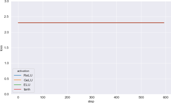
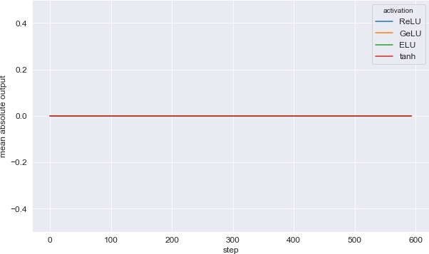
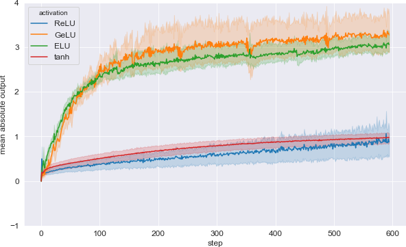
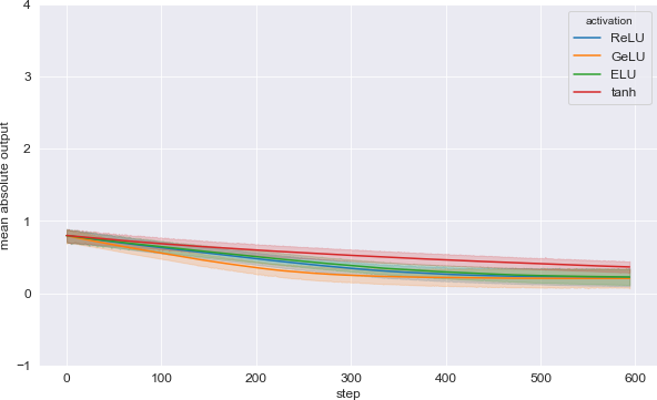
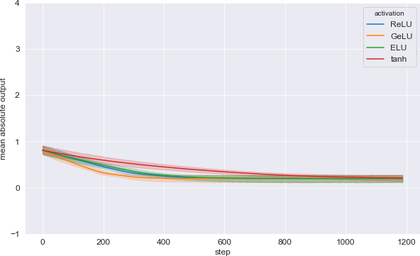
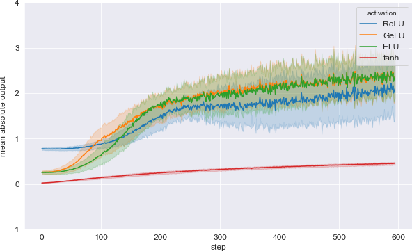
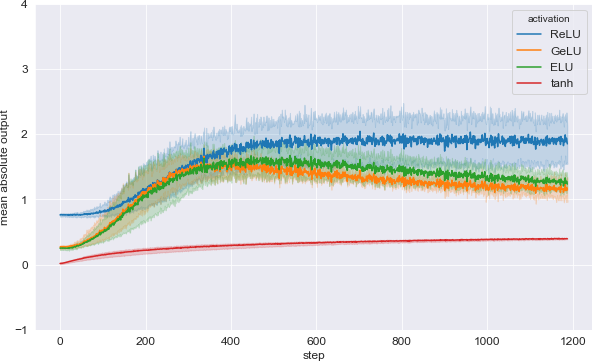
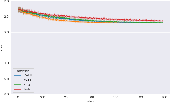
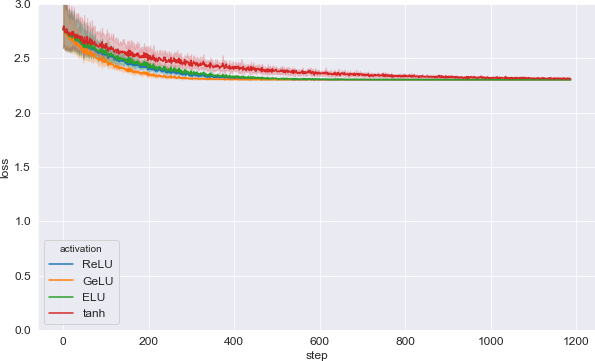
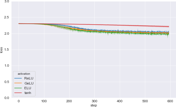
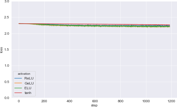
As observed in Figure 1, while the loss (averaged over a batch) stays at its initial value for Naive-IP, we observe a decrease for IP-LLR whose strength depends on the choice of activation function. Similarly, Figure 2 depicts the evolution of the mean absolute output during training, that is, we plot for any step t𝑡t the quantity (1/B)i=1B(1/10)k=110|fk,t(ξt(i))|1𝐵superscriptsubscript𝑖1𝐵110superscriptsubscript𝑘110subscript𝑓𝑘𝑡superscriptsubscript𝜉𝑡𝑖(1/B)\sum_{i=1}^{B}(1/10)\sum_{k=1}^{10}\left|f_{k,t}\left(\xi_{t}^{(i)}\right)\right|, where ξt(i)superscriptsubscript𝜉𝑡𝑖\xi_{t}^{(i)} is the i𝑖i-th sample in the batch at time t𝑡t and for any class label k[1,10]𝑘110k\in[1,10], fk,t(ξ)subscript𝑓𝑘𝑡𝜉f_{k,t}(\xi) is the k𝑘k-th entry of the output of the model (logits for class k𝑘k) on input ξ𝜉\xi. We also observe here that there is no change in the output for the Naive-IP which stays equal to 0 during the course of training, whereas for IP-LLR, the mean absolute output value increases from its initial value, equal to 0, to some positive quantity whose value depends on the activation function. The solid line in both plots denotes the mean of the metric of interest over multiple (5) random trials while the shaded area represents a 95% confidence interval around the mean. There is no shaded area for Naive-IP since the output of the network is equal to the deterministic constant 00 at any time step for large m𝑚m, as stated in Proposition 3.1.

Refer to caption
(a) Naive-IP
Refer to caption
(b) IP-LLR
Figure 1: Loss vs. number of optimization (SGD) steps on MNIST for different activation functions.
Refer to caption
(a) Naive-IP
Refer to caption
(b) IP-LLR
Figure 2: Mean absolute output vs. number of optimization (SGD) steps on MNIST for different activation functions.

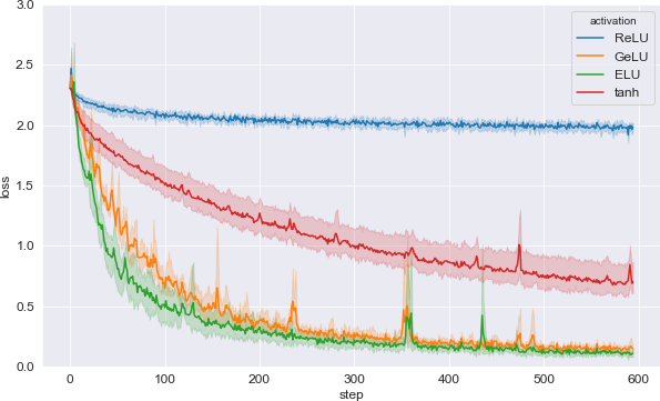
Finally, we show in Table 3 the test accuracy (averaged over 5 random runs) at the end of training for the Naive-IP and IP-LLR for different activation functions. The Naive-IP has the same test accuracy of 0.0980.0980.098 independently of the activation function, which is roughly equal to that of random guessing which would yield an accuracy of 0.100.100.10 as there are 10 classes. In contrast, IP-LLR has higher-than-chance test accuracy for every choice of activation function, and while ReLU appears to perform poorly, all other activations perform relatively well with ELU and GeLU achieving an error lower than 5%.

model activation ReLU GeLU ELU tanh
Naive-IP 0.0980.0980.098 0.0980.0980.098 0.0980.0980.098 0.0980.0980.098
IP-LLR 0.1130.1130.113 0.9560.9560.956 0.9640.9640.964 0.9320.9320.932
Table 3: Test accuracies on MNIST for various activation functions.

6.3 IP-LLR vs. μ𝜇\muP

We compare the numerical performance of IP-LLR and μ𝜇\muP on both MNIST and CIFAR-10, and investigate the reasons behind the differences observed between different models and different non-linearities.

As observed in Tables 4 and 5, the performance, as measured by the accuracy on the test set, is consistent across activation functions for μ𝜇\muP whereas the gaps are larger for IP-LLR. However, the best test accuracy for μ𝜇\muP and IP-LLR are comparable: the former achieves 0.9750.9750.975 test accuracy on MNIST and 0.4190.4190.419 test accuracy on CIFAR-10 with σ=GeLU𝜎GeLU\sigma=\text{GeLU} while the latter achieves 0.9640.9640.964 test accuracy on MNIST and 0.3830.3830.383 test accuracy on CIFAR-10 with σ=ELU𝜎ELU\sigma=\text{ELU}.

model activation ReLU GeLU ELU tanh
IP-LLR 0.1130.1130.113 0.9560.9560.956 0.9640.9640.964 0.9320.9320.932
μ𝜇\muP 0.9540.9540.954 0.9750.9750.975 0.9280.9280.928 0.9050.9050.905
Table 4: Test accuracies on MNIST for various activation functions.
model activation ReLU GeLU ELU tanh
IP-LLR 0.1000.1000.100 0.3290.3290.329 0.3830.3830.383 0.2840.2840.284
μ𝜇\muP 0.4070.4070.407 0.4190.4190.419 0.3560.3560.356 0.3040.3040.304
Table 5: Test accuracies on CIFAR-10 for various activation functions.
Performance and rank collapse.
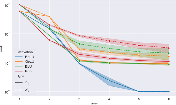
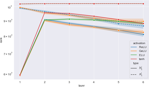
The consistency of μ𝜇\muP across activation functions and the lack of consistency for IP-LLR can be explained by (or at least correlated with) the diversity, measured in terms of rank, of the (pre-)activations at different layers on large batches of samples. Indeed, as shown in (Daneshmand et al., 2020), the rank of the family of pre-activations (considered over large batches) has a dramatic impact on the observed performance of models. In fact, the authors argue that this might be the reason behind the empirical success of batch normalization: it allows the rank of these families of pre-activations to remain large even when the number of hidden layers L𝐿L is large, whereas they show there is a collapse in the rank without the batch-normalization operation, which coincides with poor accuracy. This problem is exacerbated in IP-LLR because the contribution of the initial weight matrices (which are full-rank) vanishes after the first gradient step, thereby lowering considerably the rank of the family of pre-activations. Two effects are then at play: (1) the choice of the activation function σ𝜎\sigma can induce large differences in the rank of the family of vectors (Wl(1)σ(h))h𝒮subscriptsuperscript𝑊𝑙1𝜎𝒮\left(W^{l}(1)\sigma(h)\right)_{h\in\mathcal{S}}, where 𝒮𝒮\mathcal{S} is a large set of vectors; (2) the impact of the activation function on (1) is compounding with depth and can lead to dramatically small rank (equal to 111 in the worst case) towards the last layers of the network.

In Figures 3 we plot the rank (the y𝑦y-axis is in log-scale) of the families (h1l(ξ))ξ𝒮subscriptsubscriptsuperscript𝑙1𝜉𝜉𝒮\left(h^{l}_{1}(\xi)\right)_{\xi\in\mathcal{S}} and (x1l(ξ))ξ𝒮subscriptsubscriptsuperscript𝑥𝑙1𝜉𝜉𝒮\left(x^{l}_{1}(\xi)\right)_{\xi\in\mathcal{S}} for l[1,L]𝑙1𝐿l\in[1,L], where 𝒮𝒮\mathcal{S} is the set comprised of the first 5,000 training inputs of MNIST. The numerical “rank” is computed as in (Daneshmand et al., 2020) with torch.matrix_rank() which regards singular values below σmax×m×107subscript𝜎max𝑚superscript107\sigma_{\text{max}}\times m\times 10^{-7} as zero. We observe that for IP-LLR, the rank of those families with σ=ReLU𝜎ReLU\sigma=\text{ReLU} is one order of magnitude smaller than for other activation functions after layer l=4𝑙4l=4 and even collapses to 1 in the last layers, which might explain its poor performance, whereas for μ𝜇\muP all activation functions induce comparable ranks which remain at least on the order of 102superscript10210^{2} at any layer. We believe the latter fact is due to the non-vanishing contributions of the initial Gaussian matrices which are full-rank (with probability 1). In contrast, it would seem like IP-LLR is much more sensitive to the choice of activation function and we identify the vanishing of the contribution of the initial weights for intermediate layers as a probable cause for this effect.

Whether the difference between ReLU and other activation functions for IP-LLR is actually due to the difference between the homogeneity property with σ=ReLU𝜎ReLU\sigma=\text{ReLU} and the effective linearization property for other activation functions (as highlighted in Remark 4.2) or to other inherent characteristics of the activation functions is still an open question and we leave it for future work.

Refer to caption
(a) IP-LLR
Refer to caption
(b) μ𝜇\muP
Figure 3: Ranks (log-scale) of the families of pre-activations (h1l(ξ)subscriptsuperscript𝑙1𝜉h^{l}_{1}(\xi)) and activations (x1l(ξ)subscriptsuperscript𝑥𝑙1𝜉x^{l}_{1}(\xi)) at time t=1𝑡1t=1 on MNIST vs. layer l𝑙l for different activation functions.

6.4 Learning is Degenerate for IP-bias and IP-non-centered

In this section we show numerically that IP-non-centered and IP-bias (see Sections 5.1 and 5.2 respectively) are able to escape the initial stationary point but that the resulting dynamics do not seem effective as observed through the evolution of the training loss.

Figure 4 shows that both models are indeed able to escape the initial stationary point as the magnitude of the output evolves non-trivially during training but in contrast Figure 5, depicting the training losses on MNIST and CIFAR-10 for both models, shows that learning is very slow for those models and that the dynamics are not effective in reducing the training loss.

Additionally, as summarized in Table 6, the slow decrease of the training loss translates into poor test accuracy at the end of training comparatively with IP-LLR and μ𝜇\muP, even with the best choice of activation function.

dataset model IP-LLR μ𝜇\muP IP-bias IP-non-centered
MNIST 0.9640.9640.964 0.9750.9750.975 0.1130.1130.113 0.2090.2090.209
CIFAR-10 0.3830.3830.383 0.4190.4190.419 0.1000.1000.100 0.1540.1540.154
Table 6: Test accuracies (averaged over 5 random runs) at the end of training on MNIST and CIFAR-10. For each model, we show the maximum (averaged) accuracy over all activation functions. For each model, the activation function which performs best is the same for both datasets and the pairing model \rightarrow activation is the following: IP-LLR \rightarrow ELU, μ𝜇\muP\rightarrow GeLU, IP-bias \rightarrow GeLU, IP-non-centered \rightarrow ELU.
Refer to caption
(a) IP-bias / MNIST
Refer to caption
(b) IP-bias / CIFAR-10
Refer to caption
(c) IP-non-centered / MNIST
Refer to caption
(d) IP-non-centered / CIFAR-10
Figure 4: Mean absolute value of the output during training.
Refer to caption
(a) IP-bias / MNIST
Refer to caption
(b) IP-bias / CIFAR-10
Refer to caption
(c) IP-non-centered / MNIST
Refer to caption
(d) IP-non-centered / CIFAR-10
Figure 5: Loss vs. number of SGD steps.

7 Conclusion

Recent research has shown that the parameterization of a neural network has a dramatic impact on its training dynamics, and therefore, on the type of functions that it is able to learn. Until now, the parameterizations used by practitioners have been restricted to standard schemes which rely on the analysis of the the first forward and backward passes. In the present work, pushing the analysis beyond the first gradient step (which is made possible by the Tensor Program framework), we have studied how to train neural networks with parameterizations that enjoy radically different behaviors, such as forgetting the contribution of the initial weights after the first weight update.

The parameterizations we have analyzed, which we refer to as integrable parameterizations, have been previously described with tools from the mean-field literature, and we have deepened our understanding of these models with a different perspective. Indeed, we have shown that these parameterizations are trivial for deep networks with centered i.i.d. initialization and a constant learning rate: they are stuck at initialization. This observation led us to explore various ways to escape this initial stationary point and initiate learning. Among those methods, we found that the only one that does not lead to a degenerate behaviour is to use large learning rates for the first gradient step. We proved that in the infinite-width limit the resulting dynamic is equivalent to a modification of μ𝜇\muP where the initial weights are removed after the first gradient step. Importantly, the random fluctuations around the limit—which are ignored in the mean-field description—turn out to actually be essential for our analysis, since it is by amplifying them that we are able to escape the stationary point.

Extending our theoretical results to a more general class of activation functions requires more thorough technical work and is left as an open problem. Also, analyzing rigorously the impact of the presence or absence of the initial weight matrices on the learning behavior appears to be an interesting avenue for future research. Finally, understanding the generalization properties of IP-LLR and μ𝜇\muP remains an important open question but is beyond the scope of this paper.

Acknowledgements

Karl Hajjar and Christophe Giraud receive respectively full and partial support from the Agence Nationale de la Recherche (ANR), reference ANR-19-CHIA-0021-01 “BiSCottE”.

Appendix

Appendix A Notations

We introduce here some additional notations that will come in handy in the text and equations presented in the Appendix.

Hat matrices.

We define the following matrices and output weight vector (see Definition 2.1 for the definitions of the matrices Ulsuperscript𝑈𝑙U^{l}):

{W^1=U1W^l=m1/2Ul,l[2,L+1].casessuperscript^𝑊1superscript𝑈1otherwiseformulae-sequencesuperscript^𝑊𝑙superscript𝑚12superscript𝑈𝑙𝑙2𝐿1otherwise\displaystyle\begin{cases}\widehat{W}^{1}=U^{1}\\ \widehat{W}^{l}=m^{-1/2}U^{l},\quad l\in[2,L+1].\end{cases} (A.1)

The pre-factor in m1/2superscript𝑚12m^{-1/2} is the natural re-scaling of the i.i.d. Gaussian matrices when their input dimension grows to infinity due to the central limit theorem (CLT).

Omegas.

For any ac-parameterization, we define ω1:=ma1assignsubscript𝜔1superscript𝑚subscript𝑎1\omega_{1}:=m^{-a_{1}}, and for any l[2,L+1]𝑙2𝐿1l\in[2,L+1], ωl:=m1/2alassignsubscript𝜔𝑙superscript𝑚12subscript𝑎𝑙\omega_{l}:=m^{1/2-a_{l}}. To avoid blow-up or vanishing in the first layer, all the parameterizations we study have ω1=1subscript𝜔11\omega_{1}=1. This is the case for integrable parameterizations, the NTK parameterization and for μ𝜇\muP. For integrable parameterizations we also have ωl=m1/2subscript𝜔𝑙superscript𝑚12\omega_{l}=m^{-1/2} for l[2,L+1]𝑙2𝐿1l\in[2,L+1], but for μ𝜇\muP, ωl=1subscript𝜔𝑙1\omega_{l}=1 if l[2,L]𝑙2𝐿l\in[2,L] and ωL+1=m1/2subscript𝜔𝐿1superscript𝑚12\omega_{L+1}=m^{-1/2} (see Section B.3 for a detailed description of μ𝜇\muP).

Those ωlsubscript𝜔𝑙\omega_{l} naturally appear in the calculations as the magnitudes of the first forward pass of an ac-parameterization of a neural network. The term malsuperscript𝑚subscript𝑎𝑙m^{-a_{l}} comes from the scaling pre-factor of the effective weights, and the added m1/2superscript𝑚12m^{1/2} appears when expressing the computation in function of the naturally scaled W^lsuperscript^𝑊𝑙\widehat{W}^{l}: Wl(0)=ωlW^lsuperscript𝑊𝑙0subscript𝜔𝑙superscript^𝑊𝑙W^{l}(0)=\omega_{l}\widehat{W}^{l}.

Scalar limits.

For any scalar ω𝜔\omega which depends on m𝑚m, we denote by ω𝜔\overset{\mathrel{{{\circ}}}}{\omega} the almost sure limit (when it exists) of this scalar as m𝑚m\rightarrow\infty.

Gradients.

We define for any t𝑡t and l𝑙l,

{dhtl:=htlft(ξt)dxtl:=xtlft(ξt)dwl(t):=wl(t)ft(ξt)dbl(t):=bl(t)ft(ξt)χt:=2(yt,ft(ξt)).casesassign𝑑subscriptsuperscript𝑙𝑡subscriptsubscriptsuperscript𝑙𝑡subscript𝑓𝑡subscript𝜉𝑡otherwiseassign𝑑subscriptsuperscript𝑥𝑙𝑡subscriptsubscriptsuperscript𝑥𝑙𝑡subscript𝑓𝑡subscript𝜉𝑡otherwiseassign𝑑superscript𝑤𝑙𝑡subscriptsuperscript𝑤𝑙𝑡subscript𝑓𝑡subscript𝜉𝑡otherwiseassign𝑑superscript𝑏𝑙𝑡subscriptsuperscript𝑏𝑙𝑡subscript𝑓𝑡subscript𝜉𝑡otherwiseassignsubscript𝜒𝑡subscript2subscript𝑦𝑡subscript𝑓𝑡subscript𝜉𝑡otherwise\displaystyle\begin{cases}dh^{l}_{t}:=\nabla_{h^{l}_{t}}f_{t}(\xi_{t})\\ dx^{l}_{t}:=\nabla_{x^{l}_{t}}f_{t}(\xi_{t})\\ dw^{l}(t):=\nabla_{w^{l}(t)}f_{t}(\xi_{t})\\ db^{l}(t):=\nabla_{b^{l}(t)}f_{t}(\xi_{t})\\ \chi_{t}:=\partial_{2}\ell(y_{t},f_{t}(\xi_{t})).\end{cases}

The equations of backpropagation give:

dxtL=WL+1(t)𝑑subscriptsuperscript𝑥𝐿𝑡superscript𝑊𝐿1𝑡\displaystyle dx^{L}_{t}=W^{L+1}(t)
dwL(t)=maL+1xtL𝑑superscript𝑤𝐿𝑡superscript𝑚subscript𝑎𝐿1subscriptsuperscript𝑥𝐿𝑡\displaystyle dw^{L}(t)=m^{-a_{L+1}}x^{L}_{t}
dhtl=dxtlσ(htl)𝑑subscriptsuperscript𝑙𝑡direct-product𝑑subscriptsuperscript𝑥𝑙𝑡superscript𝜎subscriptsuperscript𝑙𝑡\displaystyle dh^{l}_{t}=dx^{l}_{t}\odot\sigma^{\prime}(h^{l}_{t})
dxtl1=(Wl(t))dhtl𝑑subscriptsuperscript𝑥𝑙1𝑡superscriptsuperscript𝑊𝑙𝑡𝑑subscriptsuperscript𝑙𝑡\displaystyle dx^{l-1}_{t}={(W^{l}(t))}^{\intercal}dh^{l}_{t}
dwl(t)=maldhtl(xtl1),𝑑superscript𝑤𝑙𝑡superscript𝑚subscript𝑎𝑙𝑑subscriptsuperscript𝑙𝑡superscriptsubscriptsuperscript𝑥𝑙1𝑡\displaystyle dw^{l}(t)=m^{-a_{l}}dh^{l}_{t}{(x^{l-1}_{t})}^{\intercal},
dbl(t)=maldhtl.𝑑superscript𝑏𝑙𝑡superscript𝑚subscript𝑎𝑙𝑑subscriptsuperscript𝑙𝑡\displaystyle db^{l}(t)=m^{-a_{l}}dh^{l}_{t}.

As noted in Definition 2.1 Remark 2.1, one has for l[1,L]𝑙1𝐿l\in[1,L],

Δwl(t)=ηmclχtdwl(t)=ηm(al+cl)χtdhtl(xtl1),Δsuperscript𝑤𝑙𝑡𝜂superscript𝑚subscript𝑐𝑙subscript𝜒𝑡𝑑superscript𝑤𝑙𝑡𝜂superscript𝑚subscript𝑎𝑙subscript𝑐𝑙subscript𝜒𝑡𝑑subscriptsuperscript𝑙𝑡superscriptsubscriptsuperscript𝑥𝑙1𝑡\displaystyle\Delta w^{l}(t)=-\eta m^{-c_{l}}\chi_{t}dw^{l}(t)=-\eta m^{-(a_{l}+c_{l})}\chi_{t}dh^{l}_{t}{(x^{l-1}_{t})}^{\intercal}, (A.2)
ΔWl(t)=malΔwl(t)=ηm(2al+cl)χtdhtl(xtl1),Δsuperscript𝑊𝑙𝑡superscript𝑚subscript𝑎𝑙Δsuperscript𝑤𝑙𝑡𝜂superscript𝑚2subscript𝑎𝑙subscript𝑐𝑙subscript𝜒𝑡𝑑subscriptsuperscript𝑙𝑡superscriptsubscriptsuperscript𝑥𝑙1𝑡\displaystyle\Delta W^{l}(t)=m^{-a_{l}}\Delta w^{l}(t)=-\eta m^{-(2a_{l}+c_{l})}\chi_{t}dh^{l}_{t}{(x^{l-1}_{t})}^{\intercal}, (A.3)
ΔBl(t)=malΔbl(t)=ηm(2al+cl)χtdhtl,Δsuperscript𝐵𝑙𝑡superscript𝑚subscript𝑎𝑙Δsuperscript𝑏𝑙𝑡𝜂superscript𝑚2subscript𝑎𝑙subscript𝑐𝑙subscript𝜒𝑡𝑑subscriptsuperscript𝑙𝑡\displaystyle\Delta B^{l}(t)=m^{-a_{l}}\Delta b^{l}(t)=-\eta m^{-(2a_{l}+c_{l})}\chi_{t}dh^{l}_{t}, (A.4)

and for l=L+1𝑙𝐿1l=L+1

ΔwL+1(t)=ηmclχtdwL+1(t)=ηm(aL+1+cL+1)χtxtL,Δsuperscript𝑤𝐿1𝑡𝜂superscript𝑚subscript𝑐𝑙subscript𝜒𝑡𝑑superscript𝑤𝐿1𝑡𝜂superscript𝑚subscript𝑎𝐿1subscript𝑐𝐿1subscript𝜒𝑡subscriptsuperscript𝑥𝐿𝑡\displaystyle\Delta w^{L+1}(t)=-\eta m^{-c_{l}}\chi_{t}dw^{L+1}(t)=-\eta m^{-(a_{L+1}+c_{L+1})}\chi_{t}x^{L}_{t}, (A.5)
ΔWL+1(t)=maL+1ΔwL+1(t)=ηm(2aL+1+cL+1)χtxtL,Δsuperscript𝑊𝐿1𝑡superscript𝑚subscript𝑎𝐿1Δsuperscript𝑤𝐿1𝑡𝜂superscript𝑚2subscript𝑎𝐿1subscript𝑐𝐿1subscript𝜒𝑡subscriptsuperscript𝑥𝐿𝑡\displaystyle\Delta W^{L+1}(t)=m^{-a_{L+1}}\Delta w^{L+1}(t)=-\eta m^{-(2a_{L+1}+c_{L+1})}\chi_{t}x^{L}_{t}, (A.6)
ΔBL+1(t)=maL+1ΔbL+1(t)=ηm(2aL+1+cL+1)χt.Δsuperscript𝐵𝐿1𝑡superscript𝑚subscript𝑎𝐿1Δsuperscript𝑏𝐿1𝑡𝜂superscript𝑚2subscript𝑎𝐿1subscript𝑐𝐿1subscript𝜒𝑡\displaystyle\Delta B^{L+1}(t)=m^{-a_{L+1}}\Delta b^{L+1}(t)=-\eta m^{-(2a_{L+1}+c_{L+1})}\chi_{t}. (A.7)
Z variables.

As described in Section B.2, the variables Z𝑍Z with a superscript will be used to denote the random variable whose law describes the evolution of all coordinates of a given vector of the forward or backward pass at a given layer in the limit m𝑚m\rightarrow\infty.

Tilde variables.

For z{htl,xtl,dhtl,dxtl}𝑧subscriptsuperscript𝑙𝑡subscriptsuperscript𝑥𝑙𝑡𝑑subscriptsuperscript𝑙𝑡𝑑subscriptsuperscript𝑥𝑙𝑡z\in\{h^{l}_{t},x^{l}_{t},dh^{l}_{t},dx^{l}_{t}\}, we will use z~~𝑧\tilde{z} to denote a variable “without scale”, i.e., such that Zz~superscript𝑍~𝑧Z^{\tilde{z}} has positive and finite variance (see Definition F.1). When we do so, we always have z=λz~𝑧𝜆~𝑧z=\lambda\tilde{z} for some scalar λ𝜆\lambda (which might depend on m𝑚m). The tilde variables of the backward pass for t1𝑡1t\geq 1 might have different expressions in different contexts or in different proofs, but we still use the same notation every time as the exact definition should always be clear from the context.

Appendix B An overview of the Tensor Program technique

The Tensor Program technique, first introduced by in Yang (2019), was initially developed to better understand the behavior at initialization of networks whose weights are initialized i.i.d. with standard Gaussians as the number of units in each layer grows to infinity. Since the output of a hidden unit in layer l2𝑙2l\geq 2 is given by q=1mWpql(0)x0,ql1superscriptsubscript𝑞1𝑚subscriptsuperscript𝑊𝑙𝑝𝑞0subscriptsuperscript𝑥𝑙10𝑞\sum_{q=1}^{m}W^{l}_{pq}(0)x^{l-1}_{0,q}, the magnitude of the weights need to be downscaled by some negative power of m𝑚m to avoid blow-up as m𝑚m\rightarrow\infty. Scalings which have naturally appeared in the literature are m1/2superscript𝑚12m^{-1/2} and m1superscript𝑚1m^{-1}, and lead to different types of limits.

Using a first version of the Tensor Program (referred to as NETSOR), it is shown in (Yang, 2019) that the output at initialization of a neural network of any architecture (fully-connected, recurrent, convolutional, with normalization, attention, …) whose weights are initialized with Wl(0)=m1/2Ulsuperscript𝑊𝑙0superscript𝑚12superscript𝑈𝑙W^{l}(0)=m^{-1/2}U^{l} for l2𝑙2l\geq 2 (i.e., al=0subscript𝑎𝑙0a_{l}=0 and bl=1/2subscript𝑏𝑙12b_{l}=1/2 for l2𝑙2l\geq 2 in the ac-parameterization) is a Gaussian process in the infinite-width limit.

Going further, and in the light of the recent literature on the neural tangent kernel, Yang (2020a) studies the first backward pass of networks initialized as above in the limit where m𝑚m\rightarrow\infty and has shown that the neural tangent kernel at initialization, defined as K(ξ,ξ¯):=θf0(θ(0);ξ),θf0(θ(0);ξ¯)assign𝐾𝜉¯𝜉subscript𝜃subscript𝑓0𝜃0𝜉subscript𝜃subscript𝑓0𝜃0¯𝜉K(\xi,\bar{\xi}):=\left<\nabla_{\theta}f_{0}(\theta(0);\xi),\nabla_{\theta}f_{0}(\theta(0);\bar{\xi})\right> converges to a deterministic limit for any architecture.

Finally, and most importantly for our work, the Tensor Program is extended in (Yang, 2020b) to cover the forward and backward passes of networks of any architecture at any time step and not just at initialization. The crucial step taken in (Yang, 2020b) is to be able to describe the evolution of quantities where both a weight matrix Wlsuperscript𝑊𝑙W^{l} and its transpose (Wl)superscriptsuperscript𝑊𝑙{(W^{l})}^{\intercal} are involved. (Yang and Hu, 2021) then applies the results and theorems of (Yang, 2020b) in the particular context of ac-parameterizations (or rather abc-parameterizations as defined by Yang and Hu, 2021) to describe the infinite-width limits of neural networks with different parameterizations.

B.1 Intuition behind the technique

To explain the intuition behind the Tensor Program technique and how it comes into play for neural networks, let us first look at the forward pass of a fully-connected network with L𝐿L hidden layers after t𝑡t steps of SGD. Assume single samples (ξ0,y0),(ξt1,yt1)subscript𝜉0subscript𝑦0subscript𝜉𝑡1subscript𝑦𝑡1(\xi_{0},y_{0}),\ldots(\xi_{t-1},y_{t-1}) are used at each step for simplicity. Consider a neural network in any ac-parameterization and an input ξ𝜉\xi to the network. Using Equation (A.3) for the updates, the forward pass of the network at time t𝑡t is given by:

ht1subscriptsuperscript1𝑡\displaystyle h^{1}_{t} =W1(0)ξηm(2a1+c1)s=0t1χs(ξsξ)dhs1absentsuperscript𝑊10𝜉𝜂superscript𝑚2subscript𝑎1subscript𝑐1superscriptsubscript𝑠0𝑡1subscript𝜒𝑠superscriptsubscript𝜉𝑠𝜉𝑑subscriptsuperscript1𝑠\displaystyle=W^{1}(0)\xi-\eta m^{-(2a_{1}+c_{1})}\sum_{s=0}^{t-1}\chi_{s}\left(\xi_{s}^{\intercal}\xi\right)dh^{1}_{s}
htlsubscriptsuperscript𝑙𝑡\displaystyle h^{l}_{t} =Wl(0)xtl1ηm(2al+cl)s=0t1χs((xsl1)xtl1)dhslabsentsuperscript𝑊𝑙0subscriptsuperscript𝑥𝑙1𝑡𝜂superscript𝑚2subscript𝑎𝑙subscript𝑐𝑙superscriptsubscript𝑠0𝑡1subscript𝜒𝑠superscriptsubscriptsuperscript𝑥𝑙1𝑠subscriptsuperscript𝑥𝑙1𝑡𝑑subscriptsuperscript𝑙𝑠\displaystyle=W^{l}(0)x^{l-1}_{t}-\eta m^{-(2a_{l}+c_{l})}\sum_{s=0}^{t-1}\chi_{s}\left((x^{l-1}_{s})^{\intercal}x^{l-1}_{t}\right)dh^{l}_{s} l[2,L]𝑙2𝐿\displaystyle l\in[2,L]
ft(ξ)subscript𝑓𝑡𝜉\displaystyle f_{t}(\xi) =(WL+1(0))xtLηm(2aL+1+cL+1)s=0t1χs(xsL)xtL.absentsuperscriptsuperscript𝑊𝐿10subscriptsuperscript𝑥𝐿𝑡𝜂superscript𝑚2subscript𝑎𝐿1subscript𝑐𝐿1superscriptsubscript𝑠0𝑡1subscript𝜒𝑠superscriptsubscriptsuperscript𝑥𝐿𝑠subscriptsuperscript𝑥𝐿𝑡\displaystyle={(W^{L+1}(0))}^{\intercal}x^{L}_{t}-\eta m^{-(2a_{L+1}+c_{L+1})}\sum_{s=0}^{t-1}\chi_{s}(x^{L}_{s})^{\intercal}x^{L}_{t}.

To understand what happens in the forward pass, one thus needs to understand the behavior of the multiplication by i.i.d. Gaussian matrices, that of vectors dhsl𝑑subscriptsuperscript𝑙𝑠dh^{l}_{s} of the backward pass as well as that of the inner products (xsl1)xtl1superscriptsubscriptsuperscript𝑥𝑙1𝑠subscriptsuperscript𝑥𝑙1𝑡(x^{l-1}_{s})^{\intercal}x^{l-1}_{t}. As m𝑚m\rightarrow\infty, the sums defining the matrix multiplications and inner products involve an infinity of terms and one must therefore understand how those quantities scale in the limit.

Before we dive into the matrix multiplications, let us look more precisely at what the vectors dhsl𝑑subscriptsuperscript𝑙𝑠dh^{l}_{s} look like. We have:

dhsl𝑑subscriptsuperscript𝑙𝑠\displaystyle dh^{l}_{s} =dxslσ(hsl)absentdirect-product𝑑subscriptsuperscript𝑥𝑙𝑠superscript𝜎subscriptsuperscript𝑙𝑠\displaystyle=dx^{l}_{s}\odot\sigma^{\prime}(h^{l}_{s})
dxsl𝑑subscriptsuperscript𝑥𝑙𝑠\displaystyle dx^{l}_{s} =(Wl+1(0))dhsl+1ηm(2al+cl)u=0sχu((dhul+1)dhsl+1)xulabsentsuperscriptsuperscript𝑊𝑙10𝑑subscriptsuperscript𝑙1𝑠𝜂superscript𝑚2subscript𝑎𝑙subscript𝑐𝑙superscriptsubscript𝑢0𝑠subscript𝜒𝑢superscript𝑑subscriptsuperscript𝑙1𝑢𝑑subscriptsuperscript𝑙1𝑠subscriptsuperscript𝑥𝑙𝑢\displaystyle={(W^{l+1}(0))}^{\intercal}dh^{l+1}_{s}-\eta m^{-(2a_{l}+c_{l})}\sum_{u=0}^{s}\chi_{u}\left((dh^{l+1}_{u})^{\intercal}dh^{l+1}_{s}\right)x^{l}_{u} l[2,L].𝑙2𝐿\displaystyle l\in[2,L].

We observe that inner products appear again, and that in contrast with the forward pass, it is now the multiplication by the transpose of i.i.d. Gaussian matrices which appears.

We already see that two main quantities appear in the calculations: The initial i.i.d. Gaussian matrices, and vectors which are generated either (i)𝑖(i) through the multiplication of another vector with a Gaussian matrix or its transpose, or (ii)𝑖𝑖(ii) through some form of non-linearity involving other vectors as well as the activation function σ𝜎\sigma and/or its derivative σsuperscript𝜎\sigma^{\prime}. Before trying to understand how the inner products behave, let us first dive into the multiplication by i.i.d. Gaussian matrices.

B.1.1 Multiplication by i.i.d. Gaussian matrices

The multiplication of a random vector by an i.i.d. Gaussian matrix can happen in two different scenarios: (i)𝑖(i) the input vector is independent of the Gaussian weights, and (ii)𝑖𝑖(ii) the input vector is correlated with the Gaussian weights, which, in the case of neural networks, will translate into saying that the transpose of the weight matrix is used somewhere to compute the input vector.

Independent input vector. Consider a list (xq)qsubscriptsubscript𝑥𝑞𝑞superscript(x_{q})_{q\in\mathbb{N}^{*}} of i.i.d. random variables with finite first and second moments, independent of Ulsuperscript𝑈𝑙U^{l}, and consider multiplying this vector by the i.i.d. Gaussian matrix Ulsuperscript𝑈𝑙U^{l}. At any finite-width m𝑚m the p𝑝p-th entry of Ulxsuperscript𝑈𝑙𝑥U^{l}x is given by

q=1mUpqlxqmm1/2𝒩(0,𝔼[x12])superscriptsubscript𝑞1𝑚subscriptsuperscript𝑈𝑙𝑝𝑞subscript𝑥𝑞𝑚similar-to-or-equalssuperscript𝑚12𝒩0𝔼delimited-[]superscriptsubscript𝑥12\displaystyle\sum_{q=1}^{m}U^{l}_{pq}x_{q}\underset{m\rightarrow\infty}{\simeq}m^{1/2}\mathcal{N}(0,\mathbb{E}[x_{1}^{2}])

The terms (Upqlxq)q1subscriptsubscriptsuperscript𝑈𝑙𝑝𝑞subscript𝑥𝑞𝑞1(U^{l}_{pq}x_{q})_{q\geq 1} are i.i.d. with mean 0 and finite variance 𝔼[x12]𝔼delimited-[]superscriptsubscript𝑥12\mathbb{E}[x_{1}^{2}] because xqsubscript𝑥𝑞x_{q} is independent of Upqlsubscriptsuperscript𝑈𝑙𝑝𝑞U^{l}_{pq}. Therefore, by a central limit argument, the sum will behave like m1/2𝒩(0,𝔼[x12])superscript𝑚12𝒩0𝔼delimited-[]superscriptsubscript𝑥12m^{1/2}\mathcal{N}(0,\mathbb{E}[x_{1}^{2}]) for large m𝑚m. It is thus natural to scale the sum by m1/2superscript𝑚12m^{-1/2}, or equivalently to consider W^l=m1/2Ulsuperscript^𝑊𝑙superscript𝑚12superscript𝑈𝑙\widehat{W}^{l}=m^{-1/2}U^{l} (as defined in Equation A.1) for matrix multiplications.

With the above result in mind, we take a look at the first forward pass at initialization of a network where all the weight matrices are initialized as Wl(0)=W^lsuperscript𝑊𝑙0superscript^𝑊𝑙W^{l}(0)=\widehat{W}^{l} (i.e., a1=0subscript𝑎10a_{1}=0, al=1/2subscript𝑎𝑙12a_{l}=1/2, l[2,L+1]𝑙2𝐿1l\in[2,L+1]). We consider an input ξd𝜉superscript𝑑\xi\in\mathbb{R}^{d} to the network and compute the pre-activations of each layer recursively. For the first layer, we get that for any p[m]𝑝delimited-[]𝑚p\in[m],

h0,p1subscriptsuperscript10𝑝\displaystyle h^{1}_{0,p} =(W^1ξ)p=(U1ξ)pabsentsubscriptsuperscript^𝑊1𝜉𝑝subscriptsuperscript𝑈1𝜉𝑝\displaystyle=(\widehat{W}^{1}\xi)_{p}=(U^{1}\xi)_{p}
=q=1dξqUpq1𝒩(0,ξ2)absentsuperscriptsubscript𝑞1𝑑subscript𝜉𝑞subscriptsuperscript𝑈1𝑝𝑞similar-to𝒩0superscriptnorm𝜉2\displaystyle=\sum_{q=1}^{d}\xi_{q}U^{1}_{pq}\sim\mathcal{N}(0,||\xi||^{2})

Since the (Upq1)qsubscriptsubscriptsuperscript𝑈1𝑝𝑞𝑞(U^{1}_{pq})_{q} are i.i.d. standard Gaussians, the linear combination above is also a Gaussian with mean 00 and variance qξq2=ξ2subscript𝑞superscriptsubscript𝜉𝑞2superscriptnorm𝜉2\sum_{q}\xi_{q}^{2}=||\xi||^{2}. Note that since the lists (Upq1)qsubscriptsubscriptsuperscript𝑈1𝑝𝑞𝑞(U^{1}_{pq})_{q} are independent for different p𝑝p, the vector h01subscriptsuperscript10h^{1}_{0} has i.i.d. coordinates all distributed as 𝒩(0,ξ2)𝒩0superscriptnorm𝜉2\mathcal{N}(0,||\xi||^{2}). We also note that adding a bias term initialized as 𝒩(0,1)𝒩01\mathcal{N}(0,1) would simply change the variance to ξ2+1superscriptnorm𝜉21||\xi||^{2}+1.

Then for the second layer we get that for any p[m]𝑝delimited-[]𝑚p\in[m]:

h0,p2=1mq=1mUpq2σ(h0,q1)mlaw𝒩(0,𝔼[σ(h0,11)2])subscriptsuperscript20𝑝1𝑚superscriptsubscript𝑞1𝑚subscriptsuperscript𝑈2𝑝𝑞𝜎subscriptsuperscript10𝑞𝑚𝑙𝑎𝑤𝒩0𝔼delimited-[]𝜎superscriptsubscriptsuperscript1012\displaystyle h^{2}_{0,p}=\frac{1}{\sqrt{m}}\sum_{q=1}^{m}U^{2}_{pq}\sigma(h^{1}_{0,q})\xrightarrow[m\rightarrow\infty]{law}\mathcal{N}(0,\mathbb{E}[\sigma(h^{1}_{0,1})^{2}])

The terms (Upq2σ(h0,q1))qsubscriptsubscriptsuperscript𝑈2𝑝𝑞𝜎subscriptsuperscript10𝑞𝑞(U^{2}_{pq}\sigma(h^{1}_{0,q}))_{q} are i.i.d. with mean zero, and by a central limit argument, we have that the coordinates of h02subscriptsuperscript20h^{2}_{0} converge in law towards 𝒩(0,𝔼[σ(h0,11)2])𝒩0𝔼delimited-[]𝜎superscriptsubscriptsuperscript1012\mathcal{N}(0,\mathbb{E}[\sigma(h^{1}_{0,1})^{2}]) where 𝔼[σ(h0,11)2])\mathbb{E}[\sigma(h^{1}_{0,1})^{2}]) is simply 𝔼[σ(Z)2])\mathbb{E}[\sigma(Z)^{2}]) with Z𝒩(0,ξ2)similar-to𝑍𝒩0superscriptnorm𝜉2Z\sim\mathcal{N}(0,||\xi||^{2}). Those coordinates are also independent (and Gaussian at any finite width m𝑚m) conditionally on h01subscriptsuperscript10h^{1}_{0} because the lists (Upq2)qsubscriptsubscriptsuperscript𝑈2𝑝𝑞𝑞(U^{2}_{pq})_{q} are independent (Gaussians) for different p𝑝p. The different coordinates of h02subscriptsuperscript20h^{2}_{0} are identically distributed at any finite width m𝑚m and remain so in the limit. They are not strictly speaking independent at finite width but the intuition is that they become so in the limit m𝑚m\rightarrow\infty as they also become Gaussian, and that is how they should be thought of in the context of the Tensor Program.

Repeating the calculations above at every layer, we can intuitively describe the forward pass in the infinite-width limit by describing the law of a single random variable Zlsubscript𝑍𝑙Z_{l} for each layer (whose law is the common law of all the coordinates of the pre-activations h0lsubscriptsuperscript𝑙0h^{l}_{0}), and by the hand-wavy calculations above, we get the following recursion for the variables Z𝑍Z:

Z1subscript𝑍1\displaystyle Z_{1} 𝒩(0,ξ2)similar-toabsent𝒩0superscriptnorm𝜉2\displaystyle\sim\mathcal{N}(0,||\xi||^{2})
Zl+1subscript𝑍𝑙1\displaystyle Z_{l+1} 𝒩(0,𝔼[σ(Zl)2]),similar-toabsent𝒩0𝔼delimited-[]𝜎superscriptsubscript𝑍𝑙2\displaystyle\sim\mathcal{N}(0,\mathbb{E}[\sigma(Z_{l})^{2}]), l[1,L]𝑙1𝐿\displaystyle l\in[1,L]

Having discussed the case where the input vectors are not correlated with the weight matrix, we now move on to the case where there is some correlation between the two.

Correlated input vector. As the simplest form of correlation, we consider a vector x=(W^l)z𝑥superscriptsuperscript^𝑊𝑙𝑧x={(\widehat{W}^{l})}^{\intercal}z where (zq)qsubscriptsubscript𝑧𝑞𝑞superscript(z_{q})_{q\in\mathbb{N}^{*}} is a list of i.i.d. random variables independent of W^lsuperscript^𝑊𝑙\widehat{W}^{l} with finite first and second moments, and we consider the result of the multiplication h=W^lxsuperscript^𝑊𝑙𝑥h=\widehat{W}^{l}x. For any p[m]𝑝delimited-[]𝑚p\in[m], we have

hpsubscript𝑝\displaystyle h_{p} =q=1mr=1mW^pqlW^rqlzrabsentsuperscriptsubscript𝑞1𝑚superscriptsubscript𝑟1𝑚subscriptsuperscript^𝑊𝑙𝑝𝑞subscriptsuperscript^𝑊𝑙𝑟𝑞subscript𝑧𝑟\displaystyle=\sum_{q=1}^{m}\sum_{r=1}^{m}\widehat{W}^{l}_{pq}\widehat{W}^{l}_{rq}z_{r}
=[1mq=1m(Upql)2]zp+1mrpzr(1mq=1mUpqlUrql)absentdelimited-[]1𝑚superscriptsubscript𝑞1𝑚superscriptsubscriptsuperscript𝑈𝑙𝑝𝑞2subscript𝑧𝑝1𝑚subscript𝑟𝑝subscript𝑧𝑟1𝑚superscriptsubscript𝑞1𝑚subscriptsuperscript𝑈𝑙𝑝𝑞subscriptsuperscript𝑈𝑙𝑟𝑞\displaystyle=\left[\frac{1}{m}\sum_{q=1}^{m}\left(U^{l}_{pq}\right)^{2}\right]z_{p}+\frac{1}{\sqrt{m}}\sum_{r\neq p}z_{r}\left(\frac{1}{\sqrt{m}}\sum_{q=1}^{m}U^{l}_{pq}U^{l}_{rq}\right)

By the law of large numbers, the first term will converge almost surely to zpsubscript𝑧𝑝z_{p} as m𝑚m\rightarrow\infty. For the second term, the intuition is that for any rp𝑟𝑝r\neq p the terms (1/m)qUpqlUrql1𝑚subscript𝑞subscriptsuperscript𝑈𝑙𝑝𝑞subscriptsuperscript𝑈𝑙𝑟𝑞(1/\sqrt{m})\sum_{q}U^{l}_{pq}U^{l}_{rq} become distributed as independent Gaussians as m𝑚m becomes large by a central limit argument. Then, by another central limit argument, intuitively, the sum over rp𝑟𝑝r\neq p should also becomes distributed as 𝒩(0,𝔼[z12])𝒩0𝔼delimited-[]superscriptsubscript𝑧12\mathcal{N}(0,\mathbb{E}[z_{1}^{2}]). In the limit m𝑚m\rightarrow\infty, we thus expect the coordinates of h=W^l(W^l)zsuperscript^𝑊𝑙superscriptsuperscript^𝑊𝑙𝑧h=\widehat{W}^{l}{(\widehat{W}^{l})}^{\intercal}z to be the sum of two terms: a first term distributed as z1subscript𝑧1z_{1} where the correlation between the entries of W^lsuperscript^𝑊𝑙\widehat{W}^{l} and (W^l)superscriptsuperscript^𝑊𝑙{(\widehat{W}^{l})}^{\intercal} comes into play, and a second term distributed as 𝒩(0,𝔼[z12])𝒩0𝔼delimited-[]superscriptsubscript𝑧12\mathcal{N}(0,\mathbb{E}[z_{1}^{2}]) which is purely Gaussian and where the correlation between the entries of W^lsuperscript^𝑊𝑙\widehat{W}^{l} and (W^l)superscriptsuperscript^𝑊𝑙{(\widehat{W}^{l})}^{\intercal} has no effect.

The aim of the Tensor Program series (Yang, 2019, 2020a, 2020b) is to formalize those intuitions into theorems and rigorous calculations. Of course, the calculations become more complex when we introduce non-linearities and consider later steps in training than the initialization, but what the Tensor Program shows is that the intuitions above still hold.

To summarize, the intuition is that in the large-width limit, the coordinates of pre-activation vectors become i.i.d. and we thus only need to track the law of a single real-valued random variable. Therefore, any average of some function of the coordinates should converge to an expectation in the limit m𝑚m\rightarrow\infty by a law of large number argument. Finally, any multiplication by W^lsuperscript^𝑊𝑙\widehat{W}^{l} yields two terms where one is purely Gaussian and the other depends on the expression of the vector that is multiplied by W^lsuperscript^𝑊𝑙\widehat{W}^{l} in function of (W^l)superscriptsuperscript^𝑊𝑙{(\widehat{W}^{l})}^{\intercal}.

B.2 Mathematical formalism

The mathematical formalism of the Tensor Program goes beyond neural network computations and describes the evolution of any computational systems (with some restrictions) in the limit m𝑚m\rightarrow\infty. The computational system is comprised of different vectors whose dimensions are equal to m𝑚m which can be generated from a set of initial vectors in various ways. The Tensor Program is defined by the sequence of mathematical operations which produce the vectors from previously generated vectors. The operations are the same at any given width m𝑚m, only the size of the vectors and matrices involved change with m𝑚m, and the aim of the Tensor Program is to provide the tools (formalism and theorems) to be able to described the behavior of the system in the limit m𝑚m\rightarrow\infty. As described in the intuitions of the previous section B.1, the coordinates of vectors in the program are roughly i.i.d. as m𝑚m\rightarrow\infty and variables Z𝑍Z are introduced to described the common law of the coordinates in the limit m𝑚m\rightarrow\infty.

Initial vectors.

Consider a set 𝒱:={v1,,vN}(m)Nassign𝒱superscript𝑣1superscript𝑣𝑁superscriptsuperscript𝑚𝑁\mathcal{V}:=\left\{v^{1},\ldots,v^{N}\right\}\in(\mathbb{R}^{m})^{N} of initial vectors such that:

  1. (i)

    the coordinates (vp)p[m]subscriptsubscript𝑣𝑝𝑝delimited-[]𝑚(v_{p})_{p\in[m]} are i.i.d. for any v𝒱𝑣𝒱v\in\mathcal{V} and any m𝑚m. We call Zvsuperscript𝑍𝑣Z^{v} a real-valued random variable whose law is the same as that of all the coordinates.

  2. (ii)

    The joint law of Z𝒱:=(Zv1,,ZvN)assignsuperscript𝑍𝒱superscript𝑍superscript𝑣1superscript𝑍superscript𝑣𝑁Z^{\mathcal{V}}:=(Z^{v^{1}},\ldots,Z^{v^{N}}) is a Gaussian 𝒩(μinit,Σinit)𝒩subscript𝜇initsubscriptΣinit\mathcal{N}\left(\mu_{\text{init}},\Sigma_{\text{init}}\right) for any m𝑚m (the variables Zvsuperscript𝑍𝑣Z^{v} do not actually depend on m𝑚m, but this is simply to say that at any width m𝑚m and for any p[m]𝑝delimited-[]𝑚p\in[m], the law of (vp1,,vpN)subscriptsuperscript𝑣1𝑝subscriptsuperscript𝑣𝑁𝑝(v^{1}_{p},\ldots,v^{N}_{p}) is the same N𝑁N-dimensional Gaussian).

Initial scalars.

Similarly, we define a list of initial scalars θ1,,θMsubscript𝜃1subscript𝜃𝑀\theta_{1},\ldots,\theta_{M} which can depend on m𝑚m and for which the only requirement is that each θrsubscript𝜃𝑟\theta_{r} converges almost surely to some finite limit θrsubscript𝜃𝑟\overset{\mathrel{{{\circ}}}}{\theta}_{r} as m𝑚m\rightarrow\infty.

Initial Gaussian matrices.

Consider a set 𝒲:={W^1,,W^P}(m×m)Passign𝒲superscript^𝑊1superscript^𝑊𝑃superscriptsuperscript𝑚𝑚𝑃\mathcal{W}:=\left\{\widehat{W}^{1},\ldots,\widehat{W}^{P}\right\}\in(\mathbb{R}^{m\times m})^{P}, such that W^pqr𝒩(0,1/m)similar-tosubscriptsuperscript^𝑊𝑟𝑝𝑞𝒩01𝑚\widehat{W}^{r}_{pq}\sim\mathcal{N}(0,1/m) i.i.d. over p,q𝑝𝑞p,q for any r𝑟r, and the (W^r)r[P]subscriptsuperscript^𝑊𝑟𝑟delimited-[]𝑃(\widehat{W}^{r})_{r\in[P]} are independent of each other and independent of the vectors in 𝒱𝒱\mathcal{V}. Since we consider a more general setting than neural networks, we do not index those matrices by l𝑙l and can have PL𝑃𝐿P\neq L but for neural networks, those initial matrices will always be the initialization of the weight matrices of the intermediate layers l[2,L]𝑙2𝐿l\in[2,L], appropriately scaled.

Generation of new vectors/scalars.

Given previously generated vectors v1,,vksuperscript𝑣1superscript𝑣𝑘v^{1},\ldots,v^{k}, previously generated scalars θ1,,θrsubscript𝜃1subscript𝜃𝑟\theta_{1},\ldots,\theta_{r}, and a non-linearity ψ(;):k×r:𝜓superscript𝑘superscript𝑟\psi(\cdot\,;\,\cdot):\mathbb{R}^{k}\times\mathbb{R}^{r}\rightarrow\mathbb{R}, we can, in the following ways, generate:

MatMul

a vector z=W^v𝑧^𝑊𝑣z=\widehat{W}v for any v{v1,,vk}𝑣superscript𝑣1superscript𝑣𝑘v\in\{v^{1},\ldots,v^{k}\} and W^𝒲^𝑊𝒲\widehat{W}\in\mathcal{W}.

NonLin

a vector z=ψ(v1,,vk;θ1,,θr)𝑧𝜓superscript𝑣1superscript𝑣𝑘subscript𝜃1subscript𝜃𝑟z=\psi(v^{1},\ldots,v^{k}\,;\,\theta_{1},\ldots,\theta_{r}) where ψ𝜓\psi is taken element-wise, i.e., zp=ψ(vp1,,vpk;θ1,,θr)subscript𝑧𝑝𝜓subscriptsuperscript𝑣1𝑝subscriptsuperscript𝑣𝑘𝑝subscript𝜃1subscript𝜃𝑟z_{p}=\psi(v^{1}_{p},\ldots,v^{k}_{p}\,;\,\theta_{1},\ldots,\theta_{r}) for any p[m]𝑝delimited-[]𝑚p\in[m] and for any m𝑚m.

Moment

a scalar ω=1mp=1mψ(vp1,,vpk;θ1,,θr)𝜔1𝑚superscriptsubscript𝑝1𝑚𝜓subscriptsuperscript𝑣1𝑝subscriptsuperscript𝑣𝑘𝑝subscript𝜃1subscript𝜃𝑟\omega=\frac{1}{m}\sum_{p=1}^{m}\psi(v^{1}_{p},\ldots,v^{k}_{p}\,;\,\theta_{1},\ldots,\theta_{r})\in\mathbb{R}.

The non-linearity used does not have to actually depend on all the previous vectors and/or scalars, but we present the operations this way for simplicity.

Given those operations, the Tensor Program framework allows to seamlessly describe the infinite-width limit of the computational system defining a given Tensor Program by tracking recursively the laws of the variables Z𝑍Z whose law represents the common law of the coordinates of a given vector. Indeed, every vector z𝑧z in the program (initial or generated using previous vectors in the program) will roughly have i.i.d. coordinates in the limit m𝑚m\rightarrow\infty, and the Tensor Program associates a real-valued random variable Zzsuperscript𝑍𝑧Z^{z} to the vector z𝑧z. Then, associated with the operations on vectors and scalars above are the following operations on the corresponding variables Z𝑍Z which come as their natural counterparts in the infinite-width limit to track the evolution of the laws of the variables Z𝑍Z:

ZInit

For initial vectors v𝒱𝑣𝒱v\in\mathcal{V}, define Z.v=0superscriptbold-.𝑍𝑣0\overset{\boldsymbol{.}}{Z}\,^{v}=0 and Z^v=Zvsuperscript^𝑍𝑣superscript𝑍𝑣\widehat{Z}^{v}=Z^{v}. The purpose of those notations will become clear in the ZMatMul section.

ZMoment

Given a scalar ω=(1/m)p=1mψ(zp1,,zpk;θ1,,θr)𝜔1𝑚superscriptsubscript𝑝1𝑚𝜓subscriptsuperscript𝑧1𝑝subscriptsuperscript𝑧𝑘𝑝subscript𝜃1subscript𝜃𝑟\omega=(1/m)\sum_{p=1}^{m}\psi(z^{1}_{p},\ldots,z^{k}_{p}\,;\,\theta_{1},\ldots,\theta_{r}), define

ω=𝔼[ψ(Zz1,,Zzk;θ1,,θ1)]𝜔𝔼delimited-[]𝜓superscript𝑍superscript𝑧1superscript𝑍superscript𝑧𝑘subscript𝜃1subscript𝜃1\displaystyle\overset{\mathrel{{{\circ}}}}{\omega}=\mathbb{E}\left[\psi(Z^{z^{1}},\ldots,Z^{z^{k}}\,;\,\overset{\mathrel{{{\circ}}}}{\theta}_{1},\ldots,\overset{\mathrel{{{\circ}}}}{\theta}_{1})\right] (B.1)
ZNonLin

Given z=ψ(z1,,zk;θ1,,θr)𝑧𝜓superscript𝑧1superscript𝑧𝑘subscript𝜃1subscript𝜃𝑟z=\psi(z^{1},\ldots,z^{k}\,;\,\theta_{1},\ldots,\theta_{r}), define:

Zz=ψ(Zz1,,Zzk;θ1,θr)superscript𝑍𝑧𝜓superscript𝑍superscript𝑧1superscript𝑍superscript𝑧𝑘subscript𝜃1subscript𝜃𝑟\displaystyle Z^{z}=\psi(Z^{z^{1}},\ldots,Z^{z^{k}}\,;\,\overset{\mathrel{{{\circ}}}}{\theta}_{1},\ldots\overset{\mathrel{{{\circ}}}}{\theta}_{r}) (B.2)
ZMatMul

Given z=W^v𝑧^𝑊𝑣z=\widehat{W}v for a previous vector v𝑣v and W^𝒲^𝑊𝒲\widehat{W}\in\mathcal{W}, Zz=Z^z+Z.zsuperscript𝑍𝑧superscript^𝑍𝑧superscriptbold-.𝑍𝑧Z^{z}=\widehat{Z}^{z}+\overset{\boldsymbol{.}}{Z}\,^{z} is the sum of two terms:

ZHat

Z^z𝒩(0,𝔼[(Zv)2])similar-tosuperscript^𝑍𝑧𝒩0𝔼delimited-[]superscriptsuperscript𝑍𝑣2\widehat{Z}^{z}\sim\mathcal{N}\left(0,\mathbb{E}\left[\left(Z^{v}\right)^{2}\right]\right) is a purely Gaussian term. Additionally, if we let 𝒲W^subscript𝒲^𝑊\mathcal{W}_{\widehat{W}} be the set of all vectors in the program of the form W^u^𝑊𝑢\widehat{W}u for some u𝑢u in the program, the vector Z𝒲W^=(Zh)h𝒲W^superscript𝑍subscript𝒲^𝑊subscriptsuperscript𝑍subscript𝒲^𝑊Z^{\mathcal{W}_{\widehat{W}}}=(Z^{h})_{h\in\mathcal{W}_{\widehat{W}}} is defined to be jointly Gaussian with covariance matrix given by:

cov(ZWx,ZWy)=𝔼[ZxZy]covsuperscript𝑍𝑊𝑥superscript𝑍𝑊𝑦𝔼delimited-[]superscript𝑍𝑥superscript𝑍𝑦\displaystyle\text{cov}(Z^{Wx},Z^{Wy})=\mathbb{E}[Z^{x}Z^{y}]

Moreover, the vector Z𝒲W^superscript𝑍subscript𝒲^𝑊Z^{\mathcal{W}_{\widehat{W}}} is defined to be mutually independent of the list of Zusuperscript𝑍𝑢Z^{u} for u𝑢u in {Z^v:v𝒱W𝒲𝒲,WW^𝒲W}conditional-setsuperscript^𝑍𝑣𝑣subscriptformulae-sequence𝑊𝒲superscript𝒲𝑊^𝑊𝒱subscript𝒲𝑊\{\widehat{Z}^{v}:v\in\mathcal{V}\cup_{W\in\mathcal{W}\cup\mathcal{W}^{\intercal},W\neq\widehat{W}}\mathcal{W}_{W}\} where 𝒲:={W^:W^𝒲}assignsuperscript𝒲conditional-setsuperscript^𝑊^𝑊𝒲\mathcal{W}^{\intercal}:=\{{\widehat{W}}^{\intercal}:\widehat{W}\in\mathcal{W}\}, and 𝒲Wsubscript𝒲𝑊\mathcal{W}_{W} is the set of vectors in the program of the form Wu𝑊𝑢Wu for some vector u𝑢u in the program.

ZDot

Z.zsuperscriptbold-.𝑍𝑧\overset{\boldsymbol{.}}{Z}\,^{z} comes from the potential interactions (correlations) between W^^𝑊\widehat{W} and W^superscript^𝑊{\widehat{W}}^{\intercal} in the computation of z𝑧z. One can always unwind the expression of Zvsuperscript𝑍𝑣Z^{v} and express it in function of the Z^W^ysuperscript^𝑍superscript^𝑊𝑦\widehat{Z}^{{\widehat{W}}^{\intercal}y} for some x𝑥x in the program, that is we can always write Zvsuperscript𝑍𝑣Z^{v} as Zv=ϕ(Z^W^y1,,Z^W^yk,Z^x1,Z^xr;θ1,,θs)superscript𝑍𝑣italic-ϕsuperscript^𝑍superscript^𝑊superscript𝑦1superscript^𝑍superscript^𝑊superscript𝑦𝑘superscript^𝑍superscript𝑥1superscript^𝑍superscript𝑥𝑟subscript𝜃1subscript𝜃𝑠Z^{v}=\phi(\widehat{Z}^{\widehat{W}^{\intercal}y^{1}},\ldots,\widehat{Z}^{\widehat{W}^{\intercal}y^{k}}\,,\widehat{Z}^{x^{1}},\ldots\widehat{Z}^{x^{r}}\,;\,\overset{\mathrel{{{\circ}}}}{\theta}_{1},\ldots,\overset{\mathrel{{{\circ}}}}{\theta}_{s}) with x1,,xrsuperscript𝑥1superscript𝑥𝑟x^{1},\ldots,x^{r} such that W^superscript^𝑊{\widehat{W}}^{\intercal} is never used in the computation of those vectors. Then, define:

Z.z=j=1k𝔼[ZvZW^yj]Zyjsuperscriptbold-.𝑍𝑧superscriptsubscript𝑗1𝑘𝔼delimited-[]superscript𝑍𝑣superscript𝑍superscript^𝑊subscript𝑦𝑗superscript𝑍subscript𝑦𝑗\displaystyle\overset{\boldsymbol{.}}{Z}\,^{z}=\sum_{j=1}^{k}\mathbb{E}\left[\frac{\partial Z^{v}}{\partial Z^{{\widehat{W}}^{\intercal}y_{j}}}\right]Z^{y_{j}} (B.3)

where Zv/ZW^yjsuperscript𝑍𝑣superscript𝑍superscript^𝑊subscript𝑦𝑗\partial Z^{v}/\partial Z^{{\widehat{W}}^{\intercal}y_{j}} is simply defined as the j𝑗j-th partial derivative of ϕitalic-ϕ\phi above when expressing Zvsuperscript𝑍𝑣Z^{v} as required for Z.bold-.𝑍\overset{\boldsymbol{.}}{Z}\,. As noted in (Yang and Hu, 2021), if ϕitalic-ϕ\phi is not everywhere differentiable, one can leverage Stein’s lemma to replace the formula in Equation (B.3) by a linear algebra formula.

Now that we have introduced the necessary concepts and described the content of a Tensor Program, we can move on to present the main theorem derived in (Yang and Hu, 2021) which connects the mathematical operations used at finite-width with the infinite-width limit of the computational system defining a Tensor Program. The “master theorem” formulated in (Yang and Hu, 2021) is surprisingly simple (although the proof is much more intricate) yet very powerful, and goes as follows (see  Yang and Hu, 2021, Theorem 7.4):

Theorem B.1 (Master Theorem).

Given a Tensor Program, for any vectors x1,,xksuperscript𝑥1superscript𝑥𝑘x^{1},\ldots,x^{k} and scalars θ1,,θrsubscript𝜃1subscript𝜃𝑟\theta_{1},\ldots,\theta_{r} in the program, and for any pseudo-Lipschitz non-linearity ψ𝜓\psi (see Definition 3.1, page 3.1), one has that:

1mp=1mψ(xp1,,xpk;θ1,,θr)ma.s.𝔼[ψ(Zx1,,Zxk;θ1,,θr)]\displaystyle\frac{1}{m}\sum_{p=1}^{m}\psi(x^{1}_{p},\ldots,x^{k}_{p}\,;\,\theta_{1},\ldots,\theta_{r})\xrightarrow[m\rightarrow\infty]{a.s.}\mathbb{E}\left[\psi\left(Z^{x^{1}},\ldots,Z^{x^{k}}\,;\,\overset{\mathrel{{{\circ}}}}{\theta}_{1},\ldots,\overset{\mathrel{{{\circ}}}}{\theta}_{r}\right)\right]
Remark B.1.
  1. 1.

    The theorem essentially states that even though the coordinates of vectors in the program are not rigorously i.i.d. ​, they appear so from the perspective of the average by a suitable non-linearity so that a law of large number type of result holds. Note that for neural networks, even though the coordinates of the (pre-)activations follow the same law when using i.i.d. initialization for the weights, it is not a priori clear that we can consider them as independent copies, and thus that we can summarize the computations using a single real-valued variable, but the master theorem shows that from the perspective of averaging, this is in fact the case in the infinite-width limit.

  2. 2.

    In (Yang and Hu, 2021), different versions of the Tensor Program are presented in the sense that different classes of non-linearities are allowed. These differences induce minor subtleties in the master theorem and in the proofs. However, most of the results in the main text of the paper require that the non-linearities be pseudo-Lipschitz (which is the stronger assumption), both in NonLin and in the master theorem. The Assumption 2 on the activation function σ𝜎\sigma and its derivative σsuperscript𝜎\sigma^{\prime} ensures that any quantity appearing in the forward or backward computation of a neural network can be expressed as pseudo-Lipschitz non-linearity.

  3. 3.

    What the Tensor Program and its master theorem show is that to understand the behavior of the computational system in the infinite-width limit, one simply needs to track the operations on the variables Z𝑍Z which mimic the recursive operations in the computational system. Then, quantities which involve sum over coordinates such as inner products between the vectors in the program (which occur in the forward and backward passes of a neural network, as well as in the computation of the neural tangent kernel), or norm computations are easily described, when properly re-normalized, through expectations involving the corresponding variables Z𝑍Z. The main difficulty is that it is actually hard (computationally and in the mathematical formulation) to track the correlations between different Z𝑍Z because, as explained in (Yang and Hu, 2021), of the necessary unwinding in the definition of Z.bold-.𝑍\overset{\boldsymbol{.}}{Z}\,, so that the computational graph associated with the operations on the variables Z𝑍Z is hard to implement in practice.

B.3 The maximal update parameterization μ𝜇\muP

We close this section by presenting briefly the maximal update parameterization considered in (Yang and Hu, 2021). To quantify the learning abilities of a given parameterization, Yang and Hu (2021) introduce the notions of feature learning and feature kernel evolution at a given layer l[1,L]𝑙1𝐿l\in[1,L], which we recall below. Both these definitions concern the large-width limit of the networks:

Definition B.1 (Feature Learning).

An ac-parameterization is said to admit feature learning at the l𝑙l-th layer if the quantity Δxtl(ξ):=xtl(ξ)x0l(ξ)assignΔsubscriptsuperscript𝑥𝑙𝑡𝜉subscriptsuperscript𝑥𝑙𝑡𝜉subscriptsuperscript𝑥𝑙0𝜉\Delta x^{l}_{t}(\xi):=x^{l}_{t}(\xi)-x^{l}_{0}(\xi) is such that there exists a training routine for which, almost surely, there exists a constant C>0𝐶0C>0 such that Δxtl(ξ)2/mCsuperscriptnormΔsubscriptsuperscript𝑥𝑙𝑡𝜉2𝑚𝐶||\Delta x^{l}_{t}(\xi)||^{2}/m\geq C for large enough m𝑚m.

Definition B.2 (Kernel Evolution).

An ac-parameterization is said to evolve the feature kernel at the l𝑙l-th layer if the quantity ΔFtl(ξ,ξ¯):=[xtl(ξ)xtl(ξ¯)x0l(ξ)x0l(ξ¯)]/massignΔsubscriptsuperscript𝐹𝑙𝑡𝜉¯𝜉delimited-[]subscriptsuperscript𝑥𝑙𝑡superscript𝜉subscriptsuperscript𝑥𝑙𝑡¯𝜉subscriptsuperscript𝑥𝑙0superscript𝜉subscriptsuperscript𝑥𝑙0¯𝜉𝑚\Delta F^{l}_{t}(\xi,\bar{\xi}):=\left[{x^{l}_{t}(\xi)}^{\intercal}x^{l}_{t}(\bar{\xi})-{x^{l}_{0}(\xi)}^{\intercal}x^{l}_{0}(\bar{\xi})\right]/m is such that there exists a training routine for which, almost surely, there exists a constant C>0𝐶0C>0 such that for large enough m𝑚m, ΔFtl(ξ,ξ¯)CΔsubscriptsuperscript𝐹𝑙𝑡𝜉¯𝜉𝐶\Delta F^{l}_{t}(\xi,\bar{\xi})\geq C.

(Yang and Hu, 2021) goes about categorizing whether different ac-parameterizations admit feature learning or not. One of the striking result presented is that there is essentially a dichotomy (depending on the values of (al,cl)l[L+1]subscriptsubscript𝑎𝑙subscript𝑐𝑙𝑙delimited-[]𝐿1(a_{l},c_{l})_{l\in[L+1]}) among ac-parameterizations: an ac-parameterization either admits feature learning (and evolves the feature kernel) or is in the kernel regime, meaning that the quantities in definitions B.1 and  B.2 converge to 00 almost surely so that in the infinite width limit, the evolution of the prediction function ftsubscript𝑓𝑡f_{t} is deterministic and depends only on the previous prediction function ft1subscript𝑓𝑡1f_{t-1} and the loss at time (t1)𝑡1(t-1) through a (deterministic) kernel K(ξ,ξ¯)=limm(x0L(ξ))x0L(ξ¯)/m𝐾𝜉¯𝜉subscript𝑚superscriptsubscriptsuperscript𝑥𝐿0𝜉subscriptsuperscript𝑥𝐿0¯𝜉𝑚K(\xi,\bar{\xi})=\lim_{m\rightarrow\infty}{(x^{L}_{0}(\xi))}^{\intercal}x^{L}_{0}(\bar{\xi})/m (or a rescaled version thereof).

The categorization result proved in (Yang and Hu, 2021) holds for a certain class of ac-parameterizations which are deemed stable and non-trivial. Stable refers to the fact that the pre-activations and output (h0lsubscriptsuperscript𝑙0h^{l}_{0} and f0(ξ)subscript𝑓0𝜉f_{0}(\xi) respectively) at initialization do not blow-up as m𝑚m\rightarrow\infty at any layer. As already hinted in Section B.1, this corresponds to having a1=0subscript𝑎10a_{1}=0 and al1/2subscript𝑎𝑙12a_{l}\geq 1/2 for l[2,L+1]𝑙2𝐿1l\in[2,L+1]. Non-trivial refers to the fact that the pre-activations of all layers do not converge to 0 almost surely as m𝑚m\rightarrow\infty at initialization. This corresponds to having a10subscript𝑎10a_{1}\leq 0 and al1/2subscript𝑎𝑙12a_{l}\leq 1/2 for l[2,L]𝑙2𝐿l\in[2,L]. It is mentioned in (Yang and Hu, 2021) that those parameterizations for which the pre-activations of the intermediate layers converge to 00 almost surely should stay at their initialization throughout the course of training, and we actually prove in Section 3, using the Tensor Program technique, that this is the case when L3𝐿3L\geq 3 in the setting where a1=0subscript𝑎10a_{1}=0 and al=1subscript𝑎𝑙1a_{l}=1 for l[2,L+1]𝑙2𝐿1l\in[2,L+1] (i.e., integrable parameterizations) unless one uses large (polynomial in m𝑚m) initial learning rates, a scenario which is not covered in (Yang and Hu, 2021). We show that in this case, integrable parameterizations are only trivial at initialization (the pre-activations of all layers except the first one converge to 00 in the infinite-width limit) and are actually in a feature learning regime at all layers after the first gradient step (t1𝑡1t\geq 1).

The maximal update parameterization μ𝜇\muP introduced in (Yang and Hu, 2021) is the result of the analysis of the values of alsubscript𝑎𝑙a_{l}, and clsubscript𝑐𝑙c_{l} for which the parameterization admits feature learning at every layer, and maximally so in the sense that if we were to reduce the value of alsubscript𝑎𝑙a_{l} then the ΔxtlΔsubscriptsuperscript𝑥𝑙𝑡\Delta x^{l}_{t} introduced in Definition B.1 or the pre-activations htlsubscriptsuperscript𝑙𝑡h^{l}_{t} would blow-up as m𝑚m\rightarrow\infty. In essence, μ𝜇\muP corresponds to the values of alsubscript𝑎𝑙a_{l}, and clsubscript𝑐𝑙c_{l} for which ΔxtlΔsubscriptsuperscript𝑥𝑙𝑡\Delta x^{l}_{t} is as large as possible (with regards to its dependency on m𝑚m) at every layer without creating any instabilities (pre-activations or updates blowing-up) in the limit m𝑚m\rightarrow\infty. A quick analysis of the updates at t=0𝑡0t=0 shows that the choice a1=0subscript𝑎10a_{1}=0, al=1/2subscript𝑎𝑙12a_{l}=1/2 for l[2,L]𝑙2𝐿l\in[2,L], and aL+1=1subscript𝑎𝐿11a_{L+1}=1 associated with cl=1subscript𝑐𝑙1c_{l}=-1 for all l[L+1]𝑙delimited-[]𝐿1l\in[L+1] achieves this, and it is rigorously shown in (Yang and Hu, 2021) that this choice of ac-parameterization induces an update such that, ΔWl(t)xtl12/m=Θ(1)superscriptnormΔsuperscript𝑊𝑙𝑡subscriptsuperscript𝑥𝑙1𝑡2𝑚Θ1||\Delta W^{l}(t)x^{l-1}_{t}||^{2}/m=\Theta(1). We thus adopt the following definition for μ𝜇\muP which is the same as in (Yang and Hu, 2021, Definition 5.1) but re-parameterized to remove the redundant b in the abc-parameterization:

Definition B.3 (μ𝜇\muP).

The maximal update parameterization μ𝜇\muP is defined by the following choice of parameterization:

a1=0,subscript𝑎10\displaystyle a_{1}=0, c1=1,subscript𝑐11\displaystyle c_{1}=-1,
al=1/2,subscript𝑎𝑙12\displaystyle a_{l}=1/2, cl=1,l[2,L],formulae-sequencesubscript𝑐𝑙1𝑙2𝐿\displaystyle c_{l}=-1,\qquad l\in[2,L],
aL+1=1,subscript𝑎𝐿11\displaystyle a_{L+1}=1, cL+1=1.subscript𝑐𝐿11\displaystyle c_{L+1}=-1.

Appendix C Useful preliminary results

We show in this section a couple of useful results which will prove helpful in the proofs.

C.1 Positive finite moments of pseudo-Lipschitz functions of Gaussians

Lemma C.1 (Positive finite moments with polynomially bounded non-linearities).

Let ϕitalic-ϕ\phi be a polynomially bounded non-linearity which is not almost everywhere 00, and let Z𝒩(0,v2)similar-to𝑍𝒩0superscript𝑣2Z\sim\mathcal{N}(0,v^{2}) with v2<superscript𝑣2v^{2}<\infty. Then, for any p+𝑝subscriptp\in\mathbb{R}_{+}:

  1. (i)

    0𝔼[|ϕ(Z)|p]<0𝔼delimited-[]superscriptitalic-ϕ𝑍𝑝0\leq\mathbb{E}[|\phi(Z)|^{p}]<\infty,

  2. (ii)

    if in addition v2>0superscript𝑣20v^{2}>0, 0<𝔼[|ϕ(Z)|p]<0𝔼delimited-[]superscriptitalic-ϕ𝑍𝑝0<\mathbb{E}[|\phi(Z)|^{p}]<\infty.

Proof.

If v2=0superscript𝑣20v^{2}=0, and then ϕ(Z)=ϕ(0)italic-ϕ𝑍italic-ϕ0\phi(Z)=\phi(0) almost surely, so that 𝔼[|ϕ(Z)|p]=|ϕ(0)|p<𝔼delimited-[]superscriptitalic-ϕ𝑍𝑝superscriptitalic-ϕ0𝑝\mathbb{E}[|\phi(Z)|^{p}]=|\phi(0)|^{p}<\infty.

Now, assume v2>0superscript𝑣20v^{2}>0. Since ϕitalic-ϕ\phi is bounded by a polynomial of some degree r>0𝑟0r>0, |ϕ(z)|C(1+|z|r)italic-ϕ𝑧𝐶1superscript𝑧𝑟|\phi(z)|\leq C(1+|z|^{r}) for some C>0𝐶0C>0. Then, |ϕ(z)|p=exp(pln(|ϕ(z)|))Cp(1+|z|r)psuperscriptitalic-ϕ𝑧𝑝𝑝italic-ϕ𝑧superscript𝐶𝑝superscript1superscript𝑧𝑟𝑝|\phi(z)|^{p}=\exp(p\ln(|\phi(z)|))\leq C^{p}(1+|z|^{r})^{p}. Since v2>0superscript𝑣20v^{2}>0, we have

𝔼[|ϕ(Z)|p]𝔼delimited-[]superscriptitalic-ϕ𝑍𝑝\displaystyle\mathbb{E}[|\phi(Z)|^{p}] =12πv2|ϕ(z)|pez2/2v2dzabsent12𝜋superscript𝑣2subscriptsuperscriptitalic-ϕ𝑧𝑝superscript𝑒superscript𝑧22superscript𝑣2differential-d𝑧\displaystyle=\frac{1}{\sqrt{2\pi v^{2}}}\int_{\mathbb{R}}|\phi(z)|^{p}e^{-z^{2}/2v^{2}}\mathrm{d}z
12πv2Cp(1+|z|r)pez2/2v2dz<.absent12𝜋superscript𝑣2subscriptsuperscript𝐶𝑝superscript1superscript𝑧𝑟𝑝superscript𝑒superscript𝑧22superscript𝑣2differential-d𝑧\displaystyle\leq\frac{1}{\sqrt{2\pi v^{2}}}\int_{\mathbb{R}}C^{p}(1+|z|^{r})^{p}e^{-z^{2}/2v^{2}}\mathrm{d}z<\infty.

Finally, since ϕitalic-ϕ\phi is not almost everywhere 00, neither is |ϕ|psuperscriptitalic-ϕ𝑝|\phi|^{p} which shows the integral in the first equality above is not 0, and gives 𝔼[|ϕ(Z)|p]>0𝔼delimited-[]superscriptitalic-ϕ𝑍𝑝0\mathbb{E}[|\phi(Z)|^{p}]>0. ∎

C.2 The Z𝑍Z dots are 0 in the first forward-backward pass

Lemma C.2 (Z.=0bold-.𝑍0\overset{\boldsymbol{.}}{Z}\,=0 in the first forward-backward pass).

Consider an ac-parameterization of an L𝐿L-hidden layer fully-connected neural network with a10subscript𝑎10a_{1}\geq 0 and al1/2subscript𝑎𝑙12a_{l}\geq 1/2 for l[2,L+1]𝑙2𝐿1l\in[2,L+1], and with a non-linearity satisfying Assumption 2. Then for any l2𝑙2l\geq 2, Z.W^lx0l1=0superscriptbold-.𝑍superscript^𝑊𝑙subscriptsuperscript𝑥𝑙100\overset{\boldsymbol{.}}{Z}\,^{\widehat{W}^{l}x^{l-1}_{0}}=0, and for any l[1,L]𝑙1𝐿l\in[1,L], Z.(W^l)dh0l=0superscriptbold-.𝑍superscriptsuperscript^𝑊𝑙𝑑subscriptsuperscript𝑙00\overset{\boldsymbol{.}}{Z}\,^{{(\widehat{W}^{l})}^{\intercal}dh^{l}_{0}}=0.

Remark C.1.

This lemma applies to the NTK, μ𝜇\muP, and integrable parameterizations (in particular IP-LLR) as well as HP and HPZ.

Proof.

Consider any ac-parameterization of a fully-connected neural network which has a10subscript𝑎10a_{1}\geq 0 and al1/2subscript𝑎𝑙12a_{l}\geq 1/2 for l[2,L+1]𝑙2𝐿1l\in[2,L+1], and with a non-linearity satisfying Assumption 2. Define ω1=ma1subscript𝜔1superscript𝑚subscript𝑎1\omega_{1}=m^{-a_{1}} and ωl=m(al1/2)subscript𝜔𝑙superscript𝑚subscript𝑎𝑙12\omega_{l}=m^{-(a_{l}-1/2)} for l2𝑙2l\geq 2, and the initial scalar αL+1:=maL+1assignsubscript𝛼𝐿1superscript𝑚subscript𝑎𝐿1\alpha_{L+1}:=m^{-a_{L+1}}. The conditions on the alsubscript𝑎𝑙a_{l} guarantee that the ωlsubscript𝜔𝑙\omega_{l} converge almost surely to either 0 or 1 and and αL+1subscript𝛼𝐿1\alpha_{L+1} converges almost surely to 0, which allows applying the rules of the Tensor Program.

For any l[2,L]𝑙2𝐿l\in[2,L], since the computation of x0l1subscriptsuperscript𝑥𝑙10x^{l-1}_{0}, and thus of Zx0l1superscript𝑍subscriptsuperscript𝑥𝑙10Z^{x^{l-1}_{0}} do not involve (W^l)superscriptsuperscript^𝑊𝑙{(\widehat{W}^{l})}^{\intercal}, Z.W^lx0l1=0superscriptbold-.𝑍superscript^𝑊𝑙subscriptsuperscript𝑥𝑙100\overset{\boldsymbol{.}}{Z}\,^{\widehat{W}^{l}x^{l-1}_{0}}=0 as per the ZDot rule of the Tensor Program. In addition, Zh1l=ω1(Z^W^1ξ+Z^v1)superscript𝑍subscriptsuperscript𝑙1subscript𝜔1superscript^𝑍superscript^𝑊1𝜉superscript^𝑍superscript𝑣1Z^{h^{l}_{1}}=\omega_{1}(\widehat{Z}^{\widehat{W}^{1}\xi}+\widehat{Z}^{v^{1}}) and by definition, Z^W^1ξ𝒩(0,ξ2)similar-tosuperscript^𝑍superscript^𝑊1𝜉𝒩0superscriptnorm𝜉2\widehat{Z}^{\widehat{W}^{1}\xi}\sim\mathcal{N}(0,||\xi||^{2}) and Z^v1𝒩(0,1)similar-tosuperscript^𝑍superscript𝑣1𝒩01\widehat{Z}^{v^{1}}\sim\mathcal{N}(0,1) are independent Gaussians, which shows that Zh1l𝒩(0,ω12(ξ2+1))similar-tosuperscript𝑍subscriptsuperscript𝑙1𝒩0superscriptsubscript𝜔12superscriptnorm𝜉21Z^{h^{l}_{1}}\sim\mathcal{N}(0,\overset{\mathrel{{{\circ}}}}{\omega}_{1}^{2}(||\xi||^{2}+1)) whose variance is finite because ω12{0,1}superscriptsubscript𝜔1201\overset{\mathrel{{{\circ}}}}{\omega}_{1}^{2}\in\{0,1\}. By Lemma C.1, this also shows that 𝔼[(Zx01)2]<𝔼delimited-[]superscriptsuperscript𝑍subscriptsuperscript𝑥102\mathbb{E}[(Z^{x^{1}_{0}})^{2}]<\infty. Let l[2,L]𝑙2𝐿l\in[2,L] and assume that 𝔼[(Zh0l1)2]<𝔼delimited-[]superscriptsuperscript𝑍subscriptsuperscript𝑙102\mathbb{E}[(Z^{h^{l-1}_{0}})^{2}]<\infty and 𝔼[(Zx0l1)2]<𝔼delimited-[]superscriptsuperscript𝑍subscriptsuperscript𝑥𝑙102\mathbb{E}[(Z^{x^{l-1}_{0}})^{2}]<\infty. We have h0l=ωlW^lx0l1+malvlsubscriptsuperscript𝑙0subscript𝜔𝑙superscript^𝑊𝑙subscriptsuperscript𝑥𝑙10superscript𝑚subscript𝑎𝑙superscript𝑣𝑙h^{l}_{0}=\omega_{l}\widehat{W}^{l}x^{l-1}_{0}+m^{-a_{l}}v^{l}. Since m2alsuperscript𝑚2subscript𝑎𝑙m^{-2a_{l}} converges to 00 almost surely, we can consider it as an initial scalar in the program, which gives by ZNonLin Zh0l=ωlZ^W^lx0l1+0×Z^v1lsuperscript𝑍subscriptsuperscript𝑙0subscript𝜔𝑙superscript^𝑍superscript^𝑊𝑙subscriptsuperscript𝑥𝑙100superscript^𝑍subscriptsuperscript𝑣𝑙1Z^{h^{l}_{0}}=\overset{\mathrel{{{\circ}}}}{\omega}_{l}\widehat{Z}^{\widehat{W}^{l}x^{l-1}_{0}}+0\times\widehat{Z}^{v^{l}_{1}}. Z^v1l𝒩(0,1)similar-tosuperscript^𝑍subscriptsuperscript𝑣𝑙1𝒩01\widehat{Z}^{v^{l}_{1}}\sim\mathcal{N}(0,1) by definition since vlsuperscript𝑣𝑙v^{l} is an initial vector in the program, so that Zh0l=ωlZ^W^lx0l1𝒩(0,ωl2𝔼[Zx0l1)2])Z^{h^{l}_{0}}=\overset{\mathrel{{{\circ}}}}{\omega}_{l}\widehat{Z}^{\widehat{W}^{l}x^{l-1}_{0}}\sim\mathcal{N}(0,\overset{\mathrel{{{\circ}}}}{\omega}_{l}^{2}\mathbb{E}[Z^{x^{l-1}_{0}})^{2}]) whose variance is finite by the induction hypothesis and because ωl{0,1}subscript𝜔𝑙01\overset{\mathrel{{{\circ}}}}{\omega}_{l}\in\{0,1\}. Then by Lemma C.1, we also get that 𝔼[(Zx0l)2]<𝔼delimited-[]superscriptsuperscript𝑍subscriptsuperscript𝑥𝑙02\mathbb{E}[(Z^{x^{l}_{0}})^{2}]<\infty, which concludes the induction.

Let us now deal with the first backward pass for any ac-parameterization. The result will essentially boil down to having the expectation of the derivatives defining the Z.bold-.𝑍\overset{\boldsymbol{.}}{Z}\, being 0 because the weight matrices are initialized with 0 mean and because of an independence argument. We have dx0L=WL+1(0)=maL+1UL+1𝑑subscriptsuperscript𝑥𝐿0superscript𝑊𝐿10superscript𝑚subscript𝑎𝐿1superscript𝑈𝐿1dx^{L}_{0}=W^{L+1}(0)=m^{-a_{L+1}}U^{L+1}, and dh0L=dx0Lσ(Zh0L)𝑑subscriptsuperscript𝐿0direct-product𝑑subscriptsuperscript𝑥𝐿0superscript𝜎superscript𝑍subscriptsuperscript𝐿0dh^{L}_{0}=dx^{L}_{0}\odot\sigma^{\prime}(Z^{h^{L}_{0}}). By ZNonLin we thus have

Zdx0Lsuperscript𝑍𝑑subscriptsuperscript𝑥𝐿0\displaystyle Z^{dx^{L}_{0}} =αL+1ZUL+1,absentsubscript𝛼𝐿1superscript𝑍superscript𝑈𝐿1\displaystyle=\overset{\mathrel{{{\circ}}}}{\alpha}_{L+1}Z^{U^{L+1}},
Zdh0Lsuperscript𝑍𝑑subscriptsuperscript𝐿0\displaystyle Z^{dh^{L}_{0}} =αL+1ZUL+1σ(Zh0L).absentsubscript𝛼𝐿1superscript𝑍superscript𝑈𝐿1superscript𝜎superscript𝑍subscriptsuperscript𝐿0\displaystyle=\overset{\mathrel{{{\circ}}}}{\alpha}_{L+1}Z^{U^{L+1}}\sigma^{\prime}(Z^{h^{L}_{0}}).

Now let l[1,L]𝑙1𝐿l\in[1,L]. dx0l1=(W^l)dh0l𝑑subscriptsuperscript𝑥𝑙10superscriptsuperscript^𝑊𝑙𝑑subscriptsuperscript𝑙0dx^{l-1}_{0}={(\widehat{W}^{l})}^{\intercal}dh^{l}_{0} gives

Z(W^l)dh0l=Z^(W^l)dh0l+Z.(W^l)dh0l,superscript𝑍superscriptsuperscript^𝑊𝑙𝑑subscriptsuperscript𝑙0superscript^𝑍superscriptsuperscript^𝑊𝑙𝑑subscriptsuperscript𝑙0superscriptbold-.𝑍superscriptsuperscript^𝑊𝑙𝑑subscriptsuperscript𝑙0\displaystyle Z^{{(\widehat{W}^{l})}^{\intercal}dh^{l}_{0}}=\widehat{Z}^{{(\widehat{W}^{l})}^{\intercal}dh^{l}_{0}}+\overset{\boldsymbol{.}}{Z}\,^{{(\widehat{W}^{l})}^{\intercal}dh^{l}_{0}},

and to understand what Z.(W^l)dh0lsuperscriptbold-.𝑍superscriptsuperscript^𝑊𝑙𝑑subscriptsuperscript𝑙0\overset{\boldsymbol{.}}{Z}\,^{{(\widehat{W}^{l})}^{\intercal}dh^{l}_{0}} is, we need to expand the expression of Zdh0lsuperscript𝑍𝑑subscriptsuperscript𝑙0Z^{dh^{l}_{0}} in function of variables which were generated with W^lsuperscript^𝑊𝑙\widehat{W}^{l}. So far, the only variable where W^lsuperscript^𝑊𝑙\widehat{W}^{l} was used is h0l=ωlW^lx0l1subscriptsuperscript𝑙0subscript𝜔𝑙superscript^𝑊𝑙subscriptsuperscript𝑥𝑙10h^{l}_{0}=\omega_{l}\widehat{W}^{l}x^{l-1}_{0} (with the convention that x00=ξ0subscriptsuperscript𝑥00subscript𝜉0x^{0}_{0}=\xi_{0}). We thus need to expand the expression of Zdh0lsuperscript𝑍𝑑subscriptsuperscript𝑙0Z^{dh^{l}_{0}} in function of Z^W^lx0l1superscript^𝑍superscript^𝑊𝑙subscriptsuperscript𝑥𝑙10\widehat{Z}^{\widehat{W}^{l}x^{l-1}_{0}}. We have, for l=L𝑙𝐿l=L

Zdh0Lsuperscript𝑍𝑑subscriptsuperscript𝐿0\displaystyle Z^{dh^{L}_{0}} =αL+1ZUL+1σ(ωLZW^lx0L1)absentsubscript𝛼𝐿1superscript𝑍superscript𝑈𝐿1superscript𝜎subscript𝜔𝐿superscript𝑍superscript^𝑊𝑙subscriptsuperscript𝑥𝐿10\displaystyle=\overset{\mathrel{{{\circ}}}}{\alpha}_{L+1}Z^{U^{L+1}}\sigma^{\prime}(\overset{\mathrel{{{\circ}}}}{\omega}_{L}Z^{\widehat{W}^{l}x^{L-1}_{0}})
=αL+1Z^UL+1σ(ωLZ^W^lx0L1),absentsubscript𝛼𝐿1superscript^𝑍superscript𝑈𝐿1superscript𝜎subscript𝜔𝐿superscript^𝑍superscript^𝑊𝑙subscriptsuperscript𝑥𝐿10\displaystyle=\overset{\mathrel{{{\circ}}}}{\alpha}_{L+1}\widehat{Z}^{U^{L+1}}\sigma^{\prime}(\overset{\mathrel{{{\circ}}}}{\omega}_{L}\widehat{Z}^{\widehat{W}^{l}x^{L-1}_{0}}),

where the last equality stems from the fact that ZW^Lx0L1=Z^W^Lx0L1superscript𝑍superscript^𝑊𝐿subscriptsuperscript𝑥𝐿10superscript^𝑍superscript^𝑊𝐿subscriptsuperscript𝑥𝐿10Z^{\widehat{W}^{L}x^{L-1}_{0}}=\widehat{Z}^{\widehat{W}^{L}x^{L-1}_{0}} in the first forward pass, and the fact that UL+1superscript𝑈𝐿1U^{L+1} is an initial vector in the program which gives by definition Z^UL+1=ZUL+1superscript^𝑍superscript𝑈𝐿1superscript𝑍superscript𝑈𝐿1\widehat{Z}^{U^{L+1}}=Z^{U^{L+1}}. We can formally write this as

Zdh0L=Ψ(Z^W^Lx0L1,Z^UL+1;αL+1,ωL),superscript𝑍𝑑subscriptsuperscript𝐿0Ψsuperscript^𝑍superscript^𝑊𝐿subscriptsuperscript𝑥𝐿10superscript^𝑍superscript𝑈𝐿1subscript𝛼𝐿1subscript𝜔𝐿\displaystyle Z^{dh^{L}_{0}}=\Psi(\widehat{Z}^{\widehat{W}^{L}x^{L-1}_{0}},\widehat{Z}^{U^{L+1}};\overset{\mathrel{{{\circ}}}}{\alpha}_{L+1},\overset{\mathrel{{{\circ}}}}{\omega}_{L}),

where Ψ(z1,z2;θ1,θ2):=θ1z2σ(θ2z1)assignΨsubscript𝑧1subscript𝑧2subscript𝜃1subscript𝜃2subscript𝜃1subscript𝑧2superscript𝜎subscript𝜃2subscript𝑧1\Psi(z_{1},z_{2};\theta_{1},\theta_{2}):=\theta_{1}z_{2}\sigma^{\prime}(\theta_{2}z_{1}) is a pseudo-Lipschitz function because σsuperscript𝜎\sigma^{\prime} is, and we have

Ψz1(z1,z2;θ1,θ2)=θ1θ2z2σ′′(θ2z1).Ψsubscript𝑧1subscript𝑧1subscript𝑧2subscript𝜃1subscript𝜃2subscript𝜃1subscript𝜃2subscript𝑧2superscript𝜎′′subscript𝜃2subscript𝑧1\displaystyle\frac{\partial\Psi}{\partial z_{1}}(z_{1},z_{2};\theta_{1},\theta_{2})=\theta_{1}\theta_{2}z_{2}\sigma^{\prime\prime}(\theta_{2}z_{1}).

We get that by definition

Z.(W^L)dh0Lsuperscriptbold-.𝑍superscriptsuperscript^𝑊𝐿𝑑subscriptsuperscript𝐿0\displaystyle\overset{\boldsymbol{.}}{Z}\,^{{(\widehat{W}^{L})}^{\intercal}dh^{L}_{0}} =𝔼[Zdh0LZ^W^Lx0L1]Zx0L1absent𝔼delimited-[]superscript𝑍𝑑subscriptsuperscript𝐿0superscript^𝑍superscript^𝑊𝐿subscriptsuperscript𝑥𝐿10superscript𝑍subscriptsuperscript𝑥𝐿10\displaystyle=\mathbb{E}\left[\frac{\partial Z^{dh^{L}_{0}}}{\partial\widehat{Z}^{\widehat{W}^{L}x^{L-1}_{0}}}\right]Z^{x^{L-1}_{0}}
=𝔼[Ψz1(Z^W^Lx0L1,Z^UL+1;αL+1,ωL)]Zx0L1absent𝔼delimited-[]Ψsubscript𝑧1superscript^𝑍superscript^𝑊𝐿subscriptsuperscript𝑥𝐿10superscript^𝑍superscript𝑈𝐿1subscript𝛼𝐿1subscript𝜔𝐿superscript𝑍subscriptsuperscript𝑥𝐿10\displaystyle=\mathbb{E}\left[\frac{\partial\Psi}{\partial z_{1}}(\widehat{Z}^{\widehat{W}^{L}x^{L-1}_{0}},\widehat{Z}^{U^{L+1}};\overset{\mathrel{{{\circ}}}}{\alpha}_{L+1},\overset{\mathrel{{{\circ}}}}{\omega}_{L})\right]Z^{x^{L-1}_{0}}
=αL+1ωL𝔼[ZUL+1σ′′(ωLZ^W^Lx0L1)]Zx0L1absentsubscript𝛼𝐿1subscript𝜔𝐿𝔼delimited-[]superscript𝑍superscript𝑈𝐿1superscript𝜎′′subscript𝜔𝐿superscript^𝑍superscript^𝑊𝐿subscriptsuperscript𝑥𝐿10superscript𝑍subscriptsuperscript𝑥𝐿10\displaystyle=\overset{\mathrel{{{\circ}}}}{\alpha}_{L+1}\overset{\mathrel{{{\circ}}}}{\omega}_{L}\mathbb{E}[Z^{U^{L+1}}\sigma^{\prime\prime}(\overset{\mathrel{{{\circ}}}}{\omega}_{L}\widehat{Z}^{\widehat{W}^{L}x^{L-1}_{0}})]Z^{x^{L-1}_{0}}
=αL+1ωL𝔼[Z^UL+1]0𝔼[σ′′(ωLZ^W^Lx0L1)]<Zx0L1<a.s.,\displaystyle=\overset{\mathrel{{{\circ}}}}{\alpha}_{L+1}\overset{\mathrel{{{\circ}}}}{\omega}_{L}\underbrace{\mathbb{E}[\widehat{Z}^{U^{L+1}}]}_{0}\underbrace{\mathbb{E}[\sigma^{\prime\prime}(\overset{\mathrel{{{\circ}}}}{\omega}_{L}\widehat{Z}^{\widehat{W}^{L}x^{L-1}_{0}})]}_{<\infty}\underbrace{Z^{x^{L-1}_{0}}}_{<\infty\ a.s.},

where the last equality stems from the fact that by ZHat, Z^W^Lx0L1superscript^𝑍superscript^𝑊𝐿subscriptsuperscript𝑥𝐿10\widehat{Z}^{\widehat{W}^{L}x^{L-1}_{0}} is independent of Z^UL+1superscript^𝑍superscript𝑈𝐿1\widehat{Z}^{U^{L+1}} because UL+1superscript𝑈𝐿1U^{L+1} is an initial vector in the program. The fact that the second expectation finite is because ωL{0,1}subscript𝜔𝐿01\overset{\mathrel{{{\circ}}}}{\omega}_{L}\in\{0,1\}, σ′′superscript𝜎′′\sigma^{\prime\prime} is polynomially bounded, and Z^W^Lx0L1superscript^𝑍superscript^𝑊𝐿subscriptsuperscript𝑥𝐿10\widehat{Z}^{\widehat{W}^{L}x^{L-1}_{0}} is a Gaussian with mean 0 and finite variance since 𝔼[(Zx0L1)2]<𝔼delimited-[]superscriptsuperscript𝑍subscriptsuperscript𝑥𝐿102\mathbb{E}[(Z^{x^{L-1}_{0}})^{2}]<\infty. This gives Z.(W^l)dh0L=0superscriptbold-.𝑍superscriptsuperscript^𝑊𝑙𝑑subscriptsuperscript𝐿00\overset{\boldsymbol{.}}{Z}\,^{{(\widehat{W}^{l})}^{\intercal}dh^{L}_{0}}=0.

Now suppose l[1,L1]𝑙1𝐿1l\in[1,L-1] and assume Z.(W^l+1)dh0l+1=0superscriptbold-.𝑍superscriptsuperscript^𝑊𝑙1𝑑subscriptsuperscript𝑙100\overset{\boldsymbol{.}}{Z}\,^{{(\widehat{W}^{l+1})}^{\intercal}dh^{l+1}_{0}}=0 which gives Z(W^l+1)dh0l+1=Z^(W^l+1)dh0l+1superscript𝑍superscriptsuperscript^𝑊𝑙1𝑑subscriptsuperscript𝑙10superscript^𝑍superscriptsuperscript^𝑊𝑙1𝑑subscriptsuperscript𝑙10Z^{{(\widehat{W}^{l+1})}^{\intercal}dh^{l+1}_{0}}=\widehat{Z}^{{(\widehat{W}^{l+1})}^{\intercal}dh^{l+1}_{0}}. We have

Zdh0lsuperscript𝑍𝑑subscriptsuperscript𝑙0\displaystyle Z^{dh^{l}_{0}} =Zdx0lσ(Zh0l)absentsuperscript𝑍𝑑subscriptsuperscript𝑥𝑙0superscript𝜎superscript𝑍subscriptsuperscript𝑙0\displaystyle=Z^{dx^{l}_{0}}\sigma^{\prime}(Z^{h^{l}_{0}})
=ωl+1Z(W^l+1)dh0l+1σ(ωlZW^lx0l1)absentsubscript𝜔𝑙1superscript𝑍superscriptsuperscript^𝑊𝑙1𝑑subscriptsuperscript𝑙10superscript𝜎subscript𝜔𝑙superscript𝑍superscript^𝑊𝑙subscriptsuperscript𝑥𝑙10\displaystyle=\overset{\mathrel{{{\circ}}}}{\omega}_{l+1}Z^{{(\widehat{W}^{l+1})}^{\intercal}dh^{l+1}_{0}}\sigma^{\prime}(\overset{\mathrel{{{\circ}}}}{\omega}_{l}Z^{\widehat{W}^{l}x^{l-1}_{0}})
=ωl+1Z^(W^l+1)dh0l+1σ(ωlZ^W^lx0l1)absentsubscript𝜔𝑙1superscript^𝑍superscriptsuperscript^𝑊𝑙1𝑑subscriptsuperscript𝑙10superscript𝜎subscript𝜔𝑙superscript^𝑍superscript^𝑊𝑙subscriptsuperscript𝑥𝑙10\displaystyle=\overset{\mathrel{{{\circ}}}}{\omega}_{l+1}\widehat{Z}^{{(\widehat{W}^{l+1})}^{\intercal}dh^{l+1}_{0}}\sigma^{\prime}(\overset{\mathrel{{{\circ}}}}{\omega}_{l}\widehat{Z}^{\widehat{W}^{l}x^{l-1}_{0}})

where we have used that previous Z.bold-.𝑍\overset{\boldsymbol{.}}{Z}\, are 0 to replace the Z𝑍Z with Z^^𝑍\widehat{Z}. We can once more formally write this as

Zdh0l=Ψ(Z^W^lx0l1,Z^(W^l+1)dh0l+1;ωl+1,ωl)superscript𝑍𝑑subscriptsuperscript𝑙0Ψsuperscript^𝑍superscript^𝑊𝑙subscriptsuperscript𝑥𝑙10superscript^𝑍superscriptsuperscript^𝑊𝑙1𝑑subscriptsuperscript𝑙10subscript𝜔𝑙1subscript𝜔𝑙\displaystyle Z^{dh^{l}_{0}}=\Psi(\widehat{Z}^{\widehat{W}^{l}x^{l-1}_{0}},\widehat{Z}^{{(\widehat{W}^{l+1})}^{\intercal}dh^{l+1}_{0}};\overset{\mathrel{{{\circ}}}}{\omega}_{l+1},\overset{\mathrel{{{\circ}}}}{\omega}_{l})

with exactly the same ΨΨ\Psi as for l=L𝑙𝐿l=L. We get that by definition

Z.(W^l)dh0lsuperscriptbold-.𝑍superscriptsuperscript^𝑊𝑙𝑑subscriptsuperscript𝑙0\displaystyle\overset{\boldsymbol{.}}{Z}\,^{{(\widehat{W}^{l})}^{\intercal}dh^{l}_{0}} =𝔼[Zdh0lZ^W^lx0l1]Zx0l1absent𝔼delimited-[]superscript𝑍𝑑subscriptsuperscript𝑙0superscript^𝑍superscript^𝑊𝑙subscriptsuperscript𝑥𝑙10superscript𝑍subscriptsuperscript𝑥𝑙10\displaystyle=\mathbb{E}\left[\frac{\partial Z^{dh^{l}_{0}}}{\partial\widehat{Z}^{\widehat{W}^{l}x^{l-1}_{0}}}\right]Z^{x^{l-1}_{0}}
=𝔼[Ψz1(Z^W^lx0l1,Z^(W^l+1)dh0l+1;ωl+1,ωl)]Zx0l1absent𝔼delimited-[]Ψsubscript𝑧1superscript^𝑍superscript^𝑊𝑙subscriptsuperscript𝑥𝑙10superscript^𝑍superscriptsuperscript^𝑊𝑙1𝑑subscriptsuperscript𝑙10subscript𝜔𝑙1subscript𝜔𝑙superscript𝑍subscriptsuperscript𝑥𝑙10\displaystyle=\mathbb{E}\left[\frac{\partial\Psi}{\partial z_{1}}(\widehat{Z}^{\widehat{W}^{l}x^{l-1}_{0}},\widehat{Z}^{{(\widehat{W}^{l+1})}^{\intercal}dh^{l+1}_{0}};\overset{\mathrel{{{\circ}}}}{\omega}_{l+1},\overset{\mathrel{{{\circ}}}}{\omega}_{l})\right]Z^{x^{l-1}_{0}}
=ωl+1ωl𝔼[Z^(W^l+1)dh0l+1σ′′(ωlZ^W^lx0l1)]Zx0l1absentsubscript𝜔𝑙1subscript𝜔𝑙𝔼delimited-[]superscript^𝑍superscriptsuperscript^𝑊𝑙1𝑑subscriptsuperscript𝑙10superscript𝜎′′subscript𝜔𝑙superscript^𝑍superscript^𝑊𝑙subscriptsuperscript𝑥𝑙10superscript𝑍subscriptsuperscript𝑥𝑙10\displaystyle=\overset{\mathrel{{{\circ}}}}{\omega}_{l+1}\overset{\mathrel{{{\circ}}}}{\omega}_{l}\mathbb{E}[\widehat{Z}^{{(\widehat{W}^{l+1})}^{\intercal}dh^{l+1}_{0}}\sigma^{\prime\prime}(\overset{\mathrel{{{\circ}}}}{\omega}_{l}\widehat{Z}^{\widehat{W}^{l}x^{l-1}_{0}})]Z^{x^{l-1}_{0}}
=ωl+1ωl𝔼[Z^(W^l+1)dh0l+1]0𝔼[σ′′(ωlZ^W^lx0l1)]<Zx0l1<a.s.\displaystyle=\overset{\mathrel{{{\circ}}}}{\omega}_{l+1}\overset{\mathrel{{{\circ}}}}{\omega}_{l}\underbrace{\mathbb{E}[\widehat{Z}^{{(\widehat{W}^{l+1})}^{\intercal}dh^{l+1}_{0}}]}_{0}\underbrace{\mathbb{E}[\sigma^{\prime\prime}(\overset{\mathrel{{{\circ}}}}{\omega}_{l}\widehat{Z}^{\widehat{W}^{l}x^{l-1}_{0}})]}_{<\infty}\underbrace{Z^{x^{l-1}_{0}}}_{<\infty a.s.}
=0absent0\displaystyle=0

Where the first expectation is 0 because by definition Z^(W^l+1)dh0l+1superscript^𝑍superscriptsuperscript^𝑊𝑙1𝑑subscriptsuperscript𝑙10\widehat{Z}^{{(\widehat{W}^{l+1})}^{\intercal}dh^{l+1}_{0}} is a Gaussian with 0 mean and an easy induction (from l=L𝑙𝐿l=L to l=1𝑙1l=1) shows that, as for the forward pass, 𝔼[(Zdx0l)2]<𝔼delimited-[]superscriptsuperscript𝑍𝑑subscriptsuperscript𝑥𝑙02\mathbb{E}[(Z^{dx^{l}_{0}})^{2}]<\infty and 𝔼[(Zdh0l)2]<𝔼delimited-[]superscriptsuperscript𝑍𝑑subscriptsuperscript𝑙02\mathbb{E}[(Z^{dh^{l}_{0}})^{2}]<\infty, which implies that Z^(W^l+1)dh0l+1superscript^𝑍superscriptsuperscript^𝑊𝑙1𝑑subscriptsuperscript𝑙10\widehat{Z}^{{(\widehat{W}^{l+1})}^{\intercal}dh^{l+1}_{0}} has finite variance. The second expectation is finite because ωl{0,1}subscript𝜔𝑙01\overset{\mathrel{{{\circ}}}}{\omega}_{l}\in\{0,1\}, Z^W^lx0l1superscript^𝑍superscript^𝑊𝑙subscriptsuperscript𝑥𝑙10\widehat{Z}^{\widehat{W}^{l}x^{l-1}_{0}} is a Gaussian with 0 mean by definition and finite variance, and because σ′′superscript𝜎′′\sigma^{\prime\prime} is polynomially bounded since σsuperscript𝜎\sigma^{\prime} is pseudo-Lipschitz. ∎

C.3 Gaussian output in the infinite-width limit

Lemma C.3 (Gaussian output).

For every m𝑚superscriptm\in\mathbb{N}^{*}, let xmsuperscript𝑥𝑚x^{m} and wmsuperscript𝑤𝑚w^{m} be independent random vectors in msuperscript𝑚\mathbb{R}^{m} such that

{1mxm2ma.s.σ2wjm𝒩(0,1/m) i.i.d. over j=1,,m.\displaystyle\begin{cases}\frac{1}{m}||x^{m}||^{2}\xrightarrow[m\rightarrow\infty]{a.s.}\sigma^{2}_{\infty}\\ w^{m}_{j}\sim\mathcal{N}(0,1/m)\text{ \text{i.i.d.~{}}over }j=1,\ldots,m.\end{cases}

Then

(wm)xmmlaw𝒩(0,σ2)𝑚𝑙𝑎𝑤superscriptsuperscript𝑤𝑚superscript𝑥𝑚𝒩0subscriptsuperscript𝜎2\displaystyle{\left(w^{m}\right)}^{\intercal}x^{m}\xrightarrow[m\rightarrow\infty]{law}\mathcal{N}(0,\sigma^{2}_{\infty})
Proof.

Consider two sequences of independent vectors of growing dimension (wm)msubscriptsuperscript𝑤𝑚𝑚(w^{m})_{m} and (xm)msubscriptsuperscript𝑥𝑚𝑚(x^{m})_{m} as in Lemma C.3. Conditionally on xmsuperscript𝑥𝑚x^{m}, the random variable (wm)xmsuperscriptsuperscript𝑤𝑚superscript𝑥𝑚{\left(w^{m}\right)}^{\intercal}x^{m} follows a Gaussian 𝒩(0,xm2/m)𝒩0superscriptnormsuperscript𝑥𝑚2𝑚\mathcal{N}(0,||x^{m}||^{2}/m) distribution. Since xm2/msuperscriptnormsuperscript𝑥𝑚2𝑚||x^{m}||^{2}/m converges to σ2subscriptsuperscript𝜎2\sigma^{2}_{\infty} almost surely, the conditional distribution of (wm)xmsuperscriptsuperscript𝑤𝑚superscript𝑥𝑚{\left(w^{m}\right)}^{\intercal}x^{m} given xmsuperscript𝑥𝑚x^{m} converges to a Gaussian 𝒩(0,σ2)𝒩0subscriptsuperscript𝜎2\mathcal{N}(0,\sigma^{2}_{\infty}) distribution. The lemma follows. ∎

C.4 Convergence of the coordinates to the limiting distribution Z𝑍Z

Lemma C.4 (Convergence to the limit distribution).

For any vector hh in the Tensor Program we have for any α𝛼superscript\alpha\in\mathbb{N}^{*},

hαmlawZh𝑚𝑙𝑎𝑤subscript𝛼superscript𝑍\displaystyle h_{\alpha}\xrightarrow[m\rightarrow\infty]{law}Z^{h}
Remark C.2.
  1. 1.

    Let h1,,hksuperscript1superscript𝑘h^{1},\ldots,h^{k} be k𝑘k vectors in the program, let θ1,,θpsubscript𝜃1subscript𝜃𝑝\theta_{1},\ldots,\theta_{p} be p𝑝p scalars in the program, and let ϕ:k+p:italic-ϕsuperscript𝑘𝑝\phi:\mathbb{R}^{k+p}\rightarrow\mathbb{R} be a pseudo-Lipschitz function. Then applying the previous Lemma C.4 to h:=ϕ(h1,,hk;θ1,,θp)assignitalic-ϕsuperscript1superscript𝑘subscript𝜃1subscript𝜃𝑝h:=\phi(h^{1},\ldots,h^{k};\theta_{1},\ldots,\theta_{p}) (which is in the program by NonLin), shows that for any α𝛼\alpha, ϕ(hα1,,hαk;θ1,,θp)italic-ϕsubscriptsuperscript1𝛼subscriptsuperscript𝑘𝛼subscript𝜃1subscript𝜃𝑝\phi(h^{1}_{\alpha},\ldots,h^{k}_{\alpha};\theta_{1},\ldots,\theta_{p}) converges in law to Zh=ϕ(Zh1,,Zhk;θ1,,θp)superscript𝑍italic-ϕsuperscript𝑍superscript1superscript𝑍superscript𝑘subscript𝜃1subscript𝜃𝑝Z^{h}=\phi(Z^{h^{1}},\ldots,Z^{h^{k}};\overset{\mathrel{{{\circ}}}}{\theta}_{1},\ldots,\overset{\mathrel{{{\circ}}}}{\theta}_{p}).

  2. 2.

    A stronger form of convergence can occur depending on the parameterization we look at and the context. Indeed, if for example Zhsuperscript𝑍Z^{h} turns out to be a constant, then we already get convergence in probability instead of in law. If in addition the convergence is “fast enough”, it can occur almost surely.

Proof.

Let hh be a vector in the program, and consider the corresponding random variable Zhsuperscript𝑍Z^{h}. All we need is to prove that for any α𝛼superscript\alpha\in\mathbb{N}^{*} and any bounded 1-Lipschitz function ϕitalic-ϕ\phi, we have 𝔼[ϕ(hα)]𝔼[ϕ(Zh)]𝔼delimited-[]italic-ϕsubscript𝛼𝔼delimited-[]italic-ϕsuperscript𝑍\mathbb{E}[\phi(h_{\alpha})]\to\mathbb{E}[\phi(Z^{h})], as m𝑚m goes to infinity. We first observe that the Master Theorem B.1 ensures the convergence

1mβ=1mϕ(hβ)ma.s.𝔼[ϕ(Zh)].\displaystyle\frac{1}{m}\sum_{\beta=1}^{m}\phi(h_{\beta})\xrightarrow[m\rightarrow\infty]{a.s.}\mathbb{E}[\phi(Z^{h})].

Secondly, for any m𝑚m, the distribution of h1,,hmsubscript1subscript𝑚h_{1},\ldots,h_{m} is exchangeable by symmetry, so that we get

𝔼[ϕ(hα)]=𝔼[1mβ=1mϕ(hβ)]m𝔼[ϕ(Zh)],𝔼delimited-[]italic-ϕsubscript𝛼𝔼delimited-[]1𝑚superscriptsubscript𝛽1𝑚italic-ϕsubscript𝛽𝑚absent𝔼delimited-[]italic-ϕsuperscript𝑍\displaystyle\mathbb{E}[\phi(h_{\alpha})]=\mathbb{E}\left[\frac{1}{m}\sum_{\beta=1}^{m}\phi(h_{\beta})\right]\xrightarrow[m\rightarrow\infty]{}\mathbb{E}[\phi(Z^{h})],

where the convergence is obtained by dominated convergence, which concludes the proof. ∎

Appendix D Proof of the triviality of IPs: Proposition 3.1

Proof.

Fix a time t0𝑡0t\geq 0 and an input ξd𝜉superscript𝑑\xi\in\mathbb{R}^{d} for the whole proof. We first show that the coordinates of the (pre-)activations of any layer l2𝑙2l\geq 2 converge to 00 almost surely at initialization. To that end, we prove that the corresponding Z𝑍Z’s are equal to 0. Then we show a similar result for the backward pass, and finally conclude the proof by an induction.

D.1 Proof at t=0𝑡0t=0

D.1.1 First forward pass

Tensor program setup: We consider a Tensor Program as defined in

{W^l+1=UL+1,U1ξ0,,U1ξt,U1ξ,v1,,vL,casessuperscript^𝑊𝑙1superscript𝑈𝐿1otherwisesuperscript𝑈1subscript𝜉0superscript𝑈1subscript𝜉𝑡superscript𝑈1𝜉otherwisesuperscript𝑣1superscript𝑣𝐿otherwise\displaystyle\begin{cases}\widehat{W}^{l+1}=U^{L+1},\\ U^{1}\xi_{0},\ldots,U^{1}\xi_{t},U^{1}\xi,\\ v^{1},\ldots,v^{L},\end{cases}

and the initial scalars

{χ0,,χt,ω:=m1/2,ν:=m1,τ:=m2,m1vL+1;casessubscript𝜒0subscript𝜒𝑡otherwiseformulae-sequenceassign𝜔superscript𝑚12formulae-sequenceassign𝜈superscript𝑚1assign𝜏superscript𝑚2otherwisesuperscript𝑚1superscript𝑣𝐿1otherwise\displaystyle\begin{cases}\chi_{0},\ldots,\chi_{t},\\ \omega:=m^{-1/2},\nu:=m^{-1},\tau:=m^{-2},\\ m^{-1}v^{L+1};\end{cases}

and with initial weight matrices

W^2,,W^L.superscript^𝑊2superscript^𝑊𝐿\displaystyle\widehat{W}^{2},\ldots,\widehat{W}^{L}.

Recall that the W^lsuperscript^𝑊𝑙\widehat{W}^{l} are defined in Equation (A.1) of Appendix A. Note that for any m𝑚superscriptm\in\mathbb{N}^{*} and j[m]𝑗delimited-[]𝑚j\in[m], we have

(UjL+1,(U1ξ0)j,,(U1ξt)j,(U1ξ)j,vj1,,vjL)𝒩(0,(1000M000IL)),similar-tosubscriptsuperscript𝑈𝐿1𝑗subscriptsuperscript𝑈1subscript𝜉0𝑗subscriptsuperscript𝑈1subscript𝜉𝑡𝑗subscriptsuperscript𝑈1𝜉𝑗subscriptsuperscript𝑣1𝑗subscriptsuperscript𝑣𝐿𝑗𝒩0matrix1000𝑀000subscript𝐼𝐿\displaystyle\left(U^{L+1}_{j},(U^{1}\xi_{0})_{j},\ldots,(U^{1}\xi_{t})_{j},(U^{1}\xi)_{j},v^{1}_{j},\ldots,v^{L}_{j}\right)\sim\mathcal{N}\left(0,\begin{pmatrix}1&0&0\\ 0&M&0\\ 0&0&I_{L}\end{pmatrix}\right),

where M:=Gram(ξ0,,ξt,ξ)=(ξrξs)0r,st+1assign𝑀Gramsubscript𝜉0subscript𝜉𝑡𝜉subscriptsuperscriptsubscript𝜉𝑟subscript𝜉𝑠formulae-sequence0𝑟𝑠𝑡1M:=\text{Gram}(\xi_{0},\ldots,\xi_{t},\xi)=(\xi_{r}^{\intercal}\xi_{s})_{0\leq r,s\leq t+1} and ILsubscript𝐼𝐿I_{L} is the identity matrix of size L×L𝐿𝐿L\times L. where we have set ξt+1:=ξassignsubscript𝜉𝑡1𝜉\xi_{t+1}:=\xi.

Convergence of the initial scalars: ω,ν,τ𝜔𝜈𝜏\omega,\nu,\tau as well as m1vL+1superscript𝑚1superscript𝑣𝐿1m^{-1}v^{L+1} all converge almost surely towards 00. For the χssubscript𝜒𝑠\chi_{s} we will show below in the proof that they all converge to constants almost surely, thereby meeting the requirements of the Tensor Program. It is important to note that there is no circular logic to prove the χssubscript𝜒𝑠\chi_{s} converge almost surely. Indeed, each time we apply the master theorem to prove the convergence of fs(ξs)subscript𝑓𝑠subscript𝜉𝑠f_{s}(\xi_{s}) to a constant almost surely and thus that of χssubscript𝜒𝑠\chi_{s}, we apply it to a restricted Tensor Program where only the scalars (χr)0r<ssubscriptsubscript𝜒𝑟0𝑟𝑠(\chi_{r})_{0\leq r<s} appear (and there is no such scalar needed to prove the convergence of χ0subscript𝜒0\chi_{0} as shown below) which will already have been proved to converge almost surely.

1st forward pass: We drop the dependency of the forward and backward passes on ξ𝜉\xi for brevity. h01=U1ξ+v1subscriptsuperscript10superscript𝑈1𝜉superscript𝑣1h^{1}_{0}=U^{1}\xi+v^{1} is th sum of two initial vectors in the program and has iid Gaussian coordinates 𝒩(0,ξ2+1)𝒩0superscriptnorm𝜉21\mathcal{N}(0,||\xi||^{2}+1). By definition, Z^h01=Z^U1ξ+Z^v1𝒩(0,ξ2+1)superscript^𝑍subscriptsuperscript10superscript^𝑍superscript𝑈1𝜉superscript^𝑍superscript𝑣1similar-to𝒩0superscriptnorm𝜉21\widehat{Z}^{h^{1}_{0}}=\widehat{Z}^{U^{1}\xi}+\widehat{Z}^{v^{1}}\sim\mathcal{N}(0,||\xi||^{2}+1) since the two Gaussians appearing in the sum are independent. By NonLin, we have that since x01=σ(h01)subscriptsuperscript𝑥10𝜎subscriptsuperscript10x^{1}_{0}=\sigma(h^{1}_{0}), Zx01=σ(Zh01)superscript𝑍subscriptsuperscript𝑥10𝜎superscript𝑍subscriptsuperscript10Z^{x^{1}_{0}}=\sigma(Z^{h^{1}_{0}}). Note that 𝔼[σ(Zh01)2]<𝔼delimited-[]𝜎superscriptsuperscript𝑍subscriptsuperscript102\mathbb{E}[\sigma(Z^{h^{1}_{0}})^{2}]<\infty since Zh01superscript𝑍subscriptsuperscript10Z^{h^{1}_{0}} is Gaussian with finite variance and σ𝜎\sigma is pseudo-Lipschitz and thus polynomially bounded.

Since L2𝐿2L\geq 2, we can write h02=m1/2W^2x01+m1v2subscriptsuperscript20superscript𝑚12superscript^𝑊2subscriptsuperscript𝑥10superscript𝑚1superscript𝑣2h^{2}_{0}=m^{-1/2}\widehat{W}^{2}x^{1}_{0}+m^{-1}v^{2} (otherwise there is no h02subscriptsuperscript20h^{2}_{0} and we simply have f0(ξ0)=m1(U2)x01subscript𝑓0subscript𝜉0superscript𝑚1superscriptsuperscript𝑈2subscriptsuperscript𝑥10f_{0}(\xi_{0})=m^{-1}{(U^{2})}^{\intercal}x^{1}_{0}), which implies by NonLin that Zh02=ωZW^2x01+νZv2superscript𝑍subscriptsuperscript20𝜔superscript𝑍superscript^𝑊2subscriptsuperscript𝑥10𝜈superscript𝑍superscript𝑣2Z^{h^{2}_{0}}=\overset{\mathrel{{{\circ}}}}{\omega}Z^{\widehat{W}^{2}x^{1}_{0}}+\overset{\mathrel{{{\circ}}}}{\nu}Z^{v^{2}} with ω=ν=0𝜔𝜈0\overset{\mathrel{{{\circ}}}}{\omega}=\overset{\mathrel{{{\circ}}}}{\nu}=0 and

ZW^2x01=Z^W^2x01+Z.W^2x01.superscript𝑍superscript^𝑊2subscriptsuperscript𝑥10superscript^𝑍superscript^𝑊2subscriptsuperscript𝑥10superscriptbold-.𝑍superscript^𝑊2subscriptsuperscript𝑥10\displaystyle Z^{\widehat{W}^{2}x^{1}_{0}}=\widehat{Z}^{\widehat{W}^{2}x^{1}_{0}}+\overset{\boldsymbol{.}}{Z}\,^{\widehat{W}^{2}x^{1}_{0}}.

Z.W^2x01=0superscriptbold-.𝑍superscript^𝑊2subscriptsuperscript𝑥100\overset{\boldsymbol{.}}{Z}\,^{\widehat{W}^{2}x^{1}_{0}}=0 by Lemma C.2, and Z^W^2x01𝒩(0,𝔼[(Zx01)2])similar-tosuperscript^𝑍superscript^𝑊2subscriptsuperscript𝑥10𝒩0𝔼delimited-[]superscriptsuperscript𝑍subscriptsuperscript𝑥102\widehat{Z}^{\widehat{W}^{2}x^{1}_{0}}\sim\mathcal{N}(0,\mathbb{E}[(Z^{x^{1}_{0}})^{2}]) and 0𝔼[(Zx01)2]<0𝔼delimited-[]superscriptsuperscript𝑍subscriptsuperscript𝑥1020\leq\mathbb{E}[(Z^{x^{1}_{0}})^{2}]<\infty. We thus have Zh02=ωZ^W^2(0)x01=0superscript𝑍subscriptsuperscript20𝜔superscript^𝑍superscript^𝑊20subscriptsuperscript𝑥100Z^{h^{2}_{0}}=\overset{\mathrel{{{\circ}}}}{\omega}\widehat{Z}^{\widehat{W}^{2}(0)x^{1}_{0}}=0. Similarly, we also get that nuZv2=0𝑛𝑢superscript𝑍superscript𝑣20\overset{\mathrel{{{\circ}}}}{\\ nu}Z^{v^{2}}=0. We then have by ZNonLin Zx02=σ(Zh02)=σ(0)=0superscript𝑍subscriptsuperscript𝑥20𝜎superscript𝑍subscriptsuperscript20𝜎00Z^{x^{2}_{0}}=\sigma(Z^{h^{2}_{0}})=\sigma(0)=0.

Let l[2,L1]𝑙2𝐿1l\in[2,L-1] and assume Zh0l=0superscript𝑍subscriptsuperscript𝑙00Z^{h^{l}_{0}}=0. Then, Zx0l=σ(Zh0l)=0superscript𝑍subscriptsuperscript𝑥𝑙0𝜎superscript𝑍subscriptsuperscript𝑙00Z^{x^{l}_{0}}=\sigma(Z^{h^{l}_{0}})=0, and since h0l+1=ωW^l+1x0l+νvl+1subscriptsuperscript𝑙10𝜔superscript^𝑊𝑙1subscriptsuperscript𝑥𝑙0𝜈superscript𝑣𝑙1h^{l+1}_{0}=\omega\widehat{W}^{l+1}x^{l}_{0}+\nu v^{l+1}, by ZNonLin, Zh0l+1=ωZW^l+1x0l+νZvl+1superscript𝑍subscriptsuperscript𝑙10𝜔superscript𝑍superscript^𝑊𝑙1subscriptsuperscript𝑥𝑙0𝜈superscript𝑍superscript𝑣𝑙1Z^{h^{l+1}_{0}}=\overset{\mathrel{{{\circ}}}}{\omega}Z^{\widehat{W}^{l+1}x^{l}_{0}}+\overset{\mathrel{{{\circ}}}}{\nu}Z^{v^{l+1}} where by ZMatMul,

ZW^l+1x0l=Z^W^l+1x0l+Z.W^l+1x0l,superscript𝑍superscript^𝑊𝑙1subscriptsuperscript𝑥𝑙0superscript^𝑍superscript^𝑊𝑙1subscriptsuperscript𝑥𝑙0superscriptbold-.𝑍superscript^𝑊𝑙1subscriptsuperscript𝑥𝑙0\displaystyle Z^{\widehat{W}^{l+1}x^{l}_{0}}=\widehat{Z}^{\widehat{W}^{l+1}x^{l}_{0}}+\overset{\boldsymbol{.}}{Z}\,^{\widehat{W}^{l+1}x^{l}_{0}},

and Z.W^l+1x0l=0superscriptbold-.𝑍superscript^𝑊𝑙1subscriptsuperscript𝑥𝑙00\overset{\boldsymbol{.}}{Z}\,^{\widehat{W}^{l+1}x^{l}_{0}}=0 by Lemma C.2. By ZHat, Z^W^l+1x0l𝒩(0,𝔼[(Zx0l)2])similar-tosuperscript^𝑍superscript^𝑊𝑙1subscriptsuperscript𝑥𝑙0𝒩0𝔼delimited-[]superscriptsuperscript𝑍subscriptsuperscript𝑥𝑙02\widehat{Z}^{\widehat{W}^{l+1}x^{l}_{0}}\sim\mathcal{N}(0,\mathbb{E}[(Z^{x^{l}_{0}})^{2}]), and since ω=0𝜔0\overset{\mathrel{{{\circ}}}}{\omega}=0, ωZ^W^l+1x0l=0𝜔superscript^𝑍superscript^𝑊𝑙1subscriptsuperscript𝑥𝑙00\overset{\mathrel{{{\circ}}}}{\omega}\widehat{Z}^{\widehat{W}^{l+1}x^{l}_{0}}=0. Similarly, νZvl+1=0𝜈superscript𝑍superscript𝑣𝑙10\overset{\mathrel{{{\circ}}}}{\nu}Z^{v^{l+1}}=0. Then, by ZNonLin Zx0l+1=σ(Zh0l+1)=σ(0)=0superscript𝑍subscriptsuperscript𝑥𝑙10𝜎superscript𝑍subscriptsuperscript𝑙10𝜎00Z^{x^{l+1}_{0}}=\sigma(Z^{h^{l+1}_{0}})=\sigma(0)=0, which concludes the induction.

We thus have only to deal with the last layer L+1𝐿1L+1 to finish the first forward pass. We have f0(ξ)=m1((UL+1(0))x0L+vL+1)=(1/m)i=1mUiL+1x0,iL+m1vL+1subscript𝑓0𝜉superscript𝑚1superscriptsuperscript𝑈𝐿10subscriptsuperscript𝑥𝐿0superscript𝑣𝐿11𝑚superscriptsubscript𝑖1𝑚subscriptsuperscript𝑈𝐿1𝑖subscriptsuperscript𝑥𝐿0𝑖superscript𝑚1superscript𝑣𝐿1f_{0}(\xi)=m^{-1}({(U^{L+1}(0))}^{\intercal}x^{L}_{0}+v^{L+1})=(1/m)\sum_{i=1}^{m}U^{L+1}_{i}x^{L}_{0,i}+m^{-1}v^{L+1}. Since UL+1superscript𝑈𝐿1U^{L+1} and x0Lsubscriptsuperscript𝑥𝐿0x^{L}_{0} are vectors in the program, (1/m)i=1mUiL+1x0,iL1𝑚superscriptsubscript𝑖1𝑚subscriptsuperscript𝑈𝐿1𝑖subscriptsuperscript𝑥𝐿0𝑖(1/m)\sum_{i=1}^{m}U^{L+1}_{i}x^{L}_{0,i} is a scalar in the program by the Moment rule, and it therefore converges almost surely to 𝔼[ZUL+1Zx0L]𝔼delimited-[]superscript𝑍superscript𝑈𝐿1superscript𝑍subscriptsuperscript𝑥𝐿0\mathbb{E}[Z^{U^{L+1}}Z^{x^{L}_{0}}] by the Master Theorem. Now because UL+1superscript𝑈𝐿1U^{L+1} is an initial vector in the program, by definition, ZUL+1=Z^UL+1𝒩(0,1)superscript𝑍superscript𝑈𝐿1superscript^𝑍superscript𝑈𝐿1similar-to𝒩01Z^{U^{L+1}}=\widehat{Z}^{U^{L+1}}\sim\mathcal{N}(0,1) is independent of Zx0Lsuperscript𝑍subscriptsuperscript𝑥𝐿0Z^{x^{L}_{0}}. We thus get 𝔼[ZUL+1Zx0L]=𝔼[ZUL+1]𝔼[Zx0L]=0𝔼delimited-[]superscript𝑍superscript𝑈𝐿1superscript𝑍subscriptsuperscript𝑥𝐿0𝔼delimited-[]superscript𝑍superscript𝑈𝐿1𝔼delimited-[]superscript𝑍subscriptsuperscript𝑥𝐿00\mathbb{E}[Z^{U^{L+1}}Z^{x^{L}_{0}}]=\mathbb{E}[Z^{U^{L+1}}]\mathbb{E}[Z^{x^{L}_{0}}]=0. On the other hand, m1vLsuperscript𝑚1superscript𝑣𝐿m^{-1}v^{L} is an initial scalar in the program which converges to 00 almost surely, so that f0(ξ)subscript𝑓0𝜉f_{0}(\xi) converges almost surely to 0.

D.1.2 First backward pass

1st backward pass: We can apply the previous reasoning of the forward pass with ξ0subscript𝜉0\xi_{0} instead of ξ𝜉\xi and we get that f0(ξ0)0subscript𝑓0subscript𝜉00f_{0}(\xi_{0})\rightarrow 0 almost surely. Therefore, since χ0=2(y0,f0(ξ0))subscript𝜒0subscript2subscript𝑦0subscript𝑓0subscript𝜉0\chi_{0}=\partial_{2}\ell(y_{0},f_{0}(\xi_{0})) and 2(y0,)subscript2subscript𝑦0\partial_{2}\ell(y_{0},\cdot) is continuous by assumption, χ02(y0,0)=:χ0\chi_{0}\rightarrow\partial_{2}\ell(y_{0},0)=:\overset{\mathrel{{{\circ}}}}{\chi}_{0} almost surely. We have dx0L=m1UL+1𝑑subscriptsuperscript𝑥𝐿0superscript𝑚1superscript𝑈𝐿1dx^{L}_{0}=m^{-1}U^{L+1} which makes it a vector in the program by NonLin, and Zdx0L=νZUL+1superscript𝑍𝑑subscriptsuperscript𝑥𝐿0𝜈superscript𝑍superscript𝑈𝐿1Z^{dx^{L}_{0}}=\overset{\mathrel{{{\circ}}}}{\nu}Z^{U^{L+1}}. Since ZUL+1𝒩(0,1)similar-tosuperscript𝑍superscript𝑈𝐿1𝒩01Z^{U^{L+1}}\sim\mathcal{N}(0,1) has finite variance and ν=0𝜈0\overset{\mathrel{{{\circ}}}}{\nu}=0, we have Zdx0L=0superscript𝑍𝑑subscriptsuperscript𝑥𝐿00Z^{dx^{L}_{0}}=0. dh0L=dx0Lσ(h0L)𝑑subscriptsuperscript𝐿0direct-product𝑑subscriptsuperscript𝑥𝐿0superscript𝜎subscriptsuperscript𝐿0dh^{L}_{0}=dx^{L}_{0}\odot\sigma^{\prime}(h^{L}_{0}) implies by ZNonLin Zdh0L=Zdx0Lσ(Zh0L)=0×σ(0)=0superscript𝑍𝑑subscriptsuperscript𝐿0superscript𝑍𝑑subscriptsuperscript𝑥𝐿0superscript𝜎superscript𝑍subscriptsuperscript𝐿00superscript𝜎00Z^{dh^{L}_{0}}=Z^{dx^{L}_{0}}\sigma^{\prime}(Z^{h^{L}_{0}})=0\times\sigma^{\prime}(0)=0.

One has:

Zmdx0L1=ω(Z^(W^L)(mdh0L)+Z.(W^L)(mdh0L)),superscript𝑍𝑚𝑑subscriptsuperscript𝑥𝐿10𝜔superscript^𝑍superscriptsuperscript^𝑊𝐿𝑚𝑑subscriptsuperscript𝐿0superscriptbold-.𝑍superscriptsuperscript^𝑊𝐿𝑚𝑑subscriptsuperscript𝐿0\displaystyle Z^{mdx^{L-1}_{0}}=\overset{\mathrel{{{\circ}}}}{\omega}(\widehat{Z}^{{(\widehat{W}^{L})}^{\intercal}(mdh^{L}_{0})}+\overset{\boldsymbol{.}}{Z}\,^{{(\widehat{W}^{L})}^{\intercal}(mdh^{L}_{0})}),

where mdh0L=UL+1σ(h0L)𝑚𝑑subscriptsuperscript𝐿0direct-productsuperscript𝑈𝐿1superscript𝜎subscriptsuperscript𝐿0mdh^{L}_{0}=U^{L+1}\odot\sigma^{\prime}(h^{L}_{0}). By Lemma C.2, Z.(W^L)(mdh0L)=0superscriptbold-.𝑍superscriptsuperscript^𝑊𝐿𝑚𝑑subscriptsuperscript𝐿00\overset{\boldsymbol{.}}{Z}\,^{{(\widehat{W}^{L})}^{\intercal}(mdh^{L}_{0})}=0 (essentially, W^lsuperscript^𝑊𝑙\widehat{W}^{l} never appears in the computation of dh0L𝑑subscriptsuperscript𝐿0dh^{L}_{0}), and by ZHat, Z^(W^L)(mdh0L)𝒩(0,𝔼[(Zmdh0L)2])similar-tosuperscript^𝑍superscriptsuperscript^𝑊𝐿𝑚𝑑subscriptsuperscript𝐿0𝒩0𝔼delimited-[]superscriptsuperscript𝑍𝑚𝑑subscriptsuperscript𝐿02\widehat{Z}^{{(\widehat{W}^{L})}^{\intercal}(mdh^{L}_{0})}\sim\mathcal{N}(0,\mathbb{E}[(Z^{mdh^{L}_{0}})^{2}]), and by independence of ZUL+1superscript𝑍superscript𝑈𝐿1Z^{U^{L+1}} and Zh0Lsuperscript𝑍subscriptsuperscript𝐿0Z^{h^{L}_{0}},

𝔼[(Zmdh0L)2])=𝔼[(ZUL+1)2])𝔼[σ(Zh0L)2])=σ(0)2\displaystyle\mathbb{E}[(Z^{mdh^{L}_{0}})^{2}])=\mathbb{E}[(Z^{U^{L+1}})^{2}])\mathbb{E}[\sigma^{\prime}(Z^{h^{L}_{0}})^{2}])=\sigma^{\prime}(0)^{2}

which is finite. Since ω=0𝜔0\overset{\mathrel{{{\circ}}}}{\omega}=0 we get Zmdx0L1=0superscript𝑍𝑚𝑑subscriptsuperscript𝑥𝐿100Z^{mdx^{L-1}_{0}}=0. dh0L1=dx0L1σ(h0L1)𝑑subscriptsuperscript𝐿10direct-product𝑑subscriptsuperscript𝑥𝐿10superscript𝜎subscriptsuperscript𝐿10dh^{L-1}_{0}=dx^{L-1}_{0}\odot\sigma^{\prime}(h^{L-1}_{0}) implies by ZNonLin Zmdh0L1=Zmdx0L1σ(Zh0L1)=0×σ(Zh0L1)=0superscript𝑍𝑚𝑑subscriptsuperscript𝐿10superscript𝑍𝑚𝑑subscriptsuperscript𝑥𝐿10superscript𝜎superscript𝑍subscriptsuperscript𝐿100superscript𝜎superscript𝑍subscriptsuperscript𝐿100Z^{mdh^{L-1}_{0}}=Z^{mdx^{L-1}_{0}}\sigma^{\prime}(Z^{h^{L-1}_{0}})=0\times\sigma^{\prime}(Z^{h^{L-1}_{0}})=0.

Let l[2,L]𝑙2𝐿l\in[2,L] (which is non-empty since L2𝐿2L\geq 2) and assume Zmdx0l=Zmdh0l=0superscript𝑍𝑚𝑑subscriptsuperscript𝑥𝑙0superscript𝑍𝑚𝑑subscriptsuperscript𝑙00Z^{mdx^{l}_{0}}=Z^{mdh^{l}_{0}}=0. mdx0l1=ω(W^l)(mdh0l)𝑚𝑑subscriptsuperscript𝑥𝑙10𝜔superscriptsuperscript^𝑊𝑙𝑚𝑑subscriptsuperscript𝑙0mdx^{l-1}_{0}=\omega{(\widehat{W}^{l})}^{\intercal}(mdh^{l}_{0}) implies by ZMatMul

Zmdx0l1=ω(Z^(W^l)(mdh0l)+Z.(W^l)(mdh0l)).superscript𝑍𝑚𝑑subscriptsuperscript𝑥𝑙10𝜔superscript^𝑍superscriptsuperscript^𝑊𝑙𝑚𝑑subscriptsuperscript𝑙0superscriptbold-.𝑍superscriptsuperscript^𝑊𝑙𝑚𝑑subscriptsuperscript𝑙0\displaystyle Z^{mdx^{l-1}_{0}}=\overset{\mathrel{{{\circ}}}}{\omega}(\widehat{Z}^{{(\widehat{W}^{l})}^{\intercal}(mdh^{l}_{0})}+\overset{\boldsymbol{.}}{Z}\,^{{(\widehat{W}^{l})}^{\intercal}(mdh^{l}_{0})}).

By Lemma C.2, Z.(W^l)(mdh0l)=0superscriptbold-.𝑍superscriptsuperscript^𝑊𝑙𝑚𝑑subscriptsuperscript𝑙00\overset{\boldsymbol{.}}{Z}\,^{{(\widehat{W}^{l})}^{\intercal}(mdh^{l}_{0})}=0, and by ZHat, Z^(W^l)(mdh0l)𝒩(0,𝔼[(Zmdh0l)2])similar-tosuperscript^𝑍superscriptsuperscript^𝑊𝑙𝑚𝑑subscriptsuperscript𝑙0𝒩0𝔼delimited-[]superscriptsuperscript𝑍𝑚𝑑subscriptsuperscript𝑙02\widehat{Z}^{{(\widehat{W}^{l})}^{\intercal}(mdh^{l}_{0})}\sim\mathcal{N}(0,\mathbb{E}[(Z^{mdh^{l}_{0}})^{2}]). By the assumption above, 𝔼[(Zmdh0l)2])=0\mathbb{E}[(Z^{mdh^{l}_{0}})^{2}])=0, and since ω=0𝜔0\overset{\mathrel{{{\circ}}}}{\omega}=0 we get Zmdx0l1=0superscript𝑍𝑚𝑑subscriptsuperscript𝑥𝑙100Z^{mdx^{l-1}_{0}}=0. dh0l1=dx0l1σ(h0l1)𝑑subscriptsuperscript𝑙10direct-product𝑑subscriptsuperscript𝑥𝑙10superscript𝜎subscriptsuperscript𝑙10dh^{l-1}_{0}=dx^{l-1}_{0}\odot\sigma^{\prime}(h^{l-1}_{0}) implies by ZNonLin Zmdh0l1=Zmdx0l1σ(Zh0l1)=0×σ(Zh0l1)superscript𝑍𝑚𝑑subscriptsuperscript𝑙10superscript𝑍𝑚𝑑subscriptsuperscript𝑥𝑙10superscript𝜎superscript𝑍subscriptsuperscript𝑙100superscript𝜎superscript𝑍subscriptsuperscript𝑙10Z^{mdh^{l-1}_{0}}=Z^{mdx^{l-1}_{0}}\sigma^{\prime}(Z^{h^{l-1}_{0}})=0\times\sigma^{\prime}(Z^{h^{l-1}_{0}}). Zh0l1superscript𝑍subscriptsuperscript𝑙10Z^{h^{l-1}_{0}} is not 00 if l=2𝑙2l=2, but since it is Gaussian with finite variance, and σsuperscript𝜎\sigma^{\prime} is pseudo-Lipschitz by assumption, σ(Zh0l1)superscript𝜎superscript𝑍subscriptsuperscript𝑙10\sigma^{\prime}(Z^{h^{l-1}_{0}}) is finite almost surely, and Zmdh0l1=0superscript𝑍𝑚𝑑subscriptsuperscript𝑙100Z^{mdh^{l-1}_{0}}=0 almost surely, which concludes the induction.

D.2 Induction step

Induction: Since we proved the result of the theorem for t=0𝑡0t=0 in the first forward pass, we might as well assume t1𝑡1t\geq 1. Let s[0,t1]𝑠0𝑡1s\in[0,t-1] be an integer. In all that follows, for any r[0,s]𝑟0𝑠r\in[0,s], for z{hrl,xrl,dhrl,dxrl}𝑧subscriptsuperscript𝑙𝑟subscriptsuperscript𝑥𝑙𝑟𝑑subscriptsuperscript𝑙𝑟𝑑subscriptsuperscript𝑥𝑙𝑟z\in\{h^{l}_{r},x^{l}_{r},dh^{l}_{r},dx^{l}_{r}\}, we use z𝑧z to denote z(ξr)𝑧subscript𝜉𝑟z(\xi_{r}). We make the following induction hypothesis: for any r[0,s]𝑟0𝑠r\in[0,s]

{Zhr1=ZU1ξr+v1𝒩(0,ξr2+1)Zhrl=0 almost surely,l[2,L]fr(ξr),fr(ξ)0 almost surely χrχr:=2(yr,0) almost surely Zmdxrl=Zmdhrl=0 almost surely,l[1,L1],ZmdxrL=UL+1.casessuperscript𝑍subscriptsuperscript1𝑟superscript𝑍superscript𝑈1subscript𝜉𝑟superscript𝑣1similar-to𝒩0superscriptnormsubscript𝜉𝑟21otherwiseformulae-sequencesuperscript𝑍subscriptsuperscript𝑙𝑟0 almost surely𝑙2𝐿otherwisesubscript𝑓𝑟subscript𝜉𝑟subscript𝑓𝑟𝜉0 almost surely otherwisesubscript𝜒𝑟subscript𝜒𝑟assignsubscript2subscript𝑦𝑟0 almost surely otherwiseformulae-sequencesuperscript𝑍𝑚𝑑subscriptsuperscript𝑥𝑙𝑟superscript𝑍𝑚𝑑subscriptsuperscript𝑙𝑟0 almost surely𝑙1𝐿1otherwisesuperscript𝑍𝑚𝑑subscriptsuperscript𝑥𝐿𝑟superscript𝑈𝐿1otherwise\displaystyle\begin{cases}Z^{h^{1}_{r}}=Z^{U^{1}\xi_{r}+v^{1}}\sim\mathcal{N}(0,||\xi_{r}||^{2}+1)\\ Z^{h^{l}_{r}}=0\ \text{ almost surely},\ l\in[2,L]\\ f_{r}(\xi_{r}),f_{r}(\xi)\rightarrow 0\ \text{ almost surely }\\ \chi_{r}\rightarrow\overset{\mathrel{{{\circ}}}}{\chi}_{r}:=\partial_{2}\ell(y_{r},0)\ \text{ almost surely }\\ Z^{mdx^{l}_{r}}=Z^{mdh^{l}_{r}}=0\ \text{ almost surely},\ l\in[1,L-1],\\ Z^{mdx^{L}_{r}}=U^{L+1}.\end{cases}

The aim is then to prove the same claims for r=s+1𝑟𝑠1r=s+1. Let us first start with the expressions of ΔWl(s+1)Δsuperscript𝑊𝑙𝑠1\Delta W^{l}(s+1) and ΔBl(s+1)Δsuperscript𝐵𝑙𝑠1\Delta B^{l}(s+1). We will use Equation (A.3) and the fact that cl+20subscript𝑐𝑙20c_{l}+2\geq 0 if l[2,L]𝑙2𝐿l\in[2,L], and cl+10subscript𝑐𝑙10c_{l}+1\geq 0 for l=1𝑙1l=1, and l=L+1𝑙𝐿1l=L+1. We have by Equations (A.3) and (A.6)

ΔW1(s+1)=ηmclr=0sχrdhr1ξr,Δsuperscript𝑊1𝑠1𝜂superscript𝑚subscript𝑐𝑙superscriptsubscript𝑟0𝑠subscript𝜒𝑟𝑑subscriptsuperscript1𝑟superscriptsubscript𝜉𝑟\displaystyle\Delta W^{1}(s+1)=-\eta m^{-c_{l}}\sum_{r=0}^{s}\chi_{r}dh^{1}_{r}\xi_{r}^{\intercal},
ΔWl(s+1)=ηm(2+cl)r=0sχrdhrl(xrl1),l[2,L],formulae-sequenceΔsuperscript𝑊𝑙𝑠1𝜂superscript𝑚2subscript𝑐𝑙superscriptsubscript𝑟0𝑠subscript𝜒𝑟𝑑subscriptsuperscript𝑙𝑟superscriptsubscriptsuperscript𝑥𝑙1𝑟𝑙2𝐿\displaystyle\Delta W^{l}(s+1)=-\eta m^{-(2+c_{l})}\sum_{r=0}^{s}\chi_{r}dh^{l}_{r}{(x^{l-1}_{r})}^{\intercal},\quad l\in[2,L],
ΔWL+1(s+1)=ηm(1+cL+1)r=0sχrxrL/m,Δsuperscript𝑊𝐿1𝑠1𝜂superscript𝑚1subscript𝑐𝐿1superscriptsubscript𝑟0𝑠subscript𝜒𝑟subscriptsuperscript𝑥𝐿𝑟𝑚\displaystyle\Delta W^{L+1}(s+1)=-\eta m^{-(1+c_{L+1})}\sum_{r=0}^{s}\chi_{r}x^{L}_{r}/m,

and by Equations (A.4) and (A.7)

ΔB1(s+1)=ηmclr=0sχrdhr1,Δsuperscript𝐵1𝑠1𝜂superscript𝑚subscript𝑐𝑙superscriptsubscript𝑟0𝑠subscript𝜒𝑟𝑑subscriptsuperscript1𝑟\displaystyle\Delta B^{1}(s+1)=-\eta m^{-c_{l}}\sum_{r=0}^{s}\chi_{r}dh^{1}_{r},
ΔBl(s+1)=ηm(2+cl)r=0sχrdhrl,l[2,L],formulae-sequenceΔsuperscript𝐵𝑙𝑠1𝜂superscript𝑚2subscript𝑐𝑙superscriptsubscript𝑟0𝑠subscript𝜒𝑟𝑑subscriptsuperscript𝑙𝑟𝑙2𝐿\displaystyle\Delta B^{l}(s+1)=-\eta m^{-(2+c_{l})}\sum_{r=0}^{s}\chi_{r}dh^{l}_{r},\quad l\in[2,L],
ΔBL+1(s+1)=ηm(1+cL+1)r=0sχr/m.Δsuperscript𝐵𝐿1𝑠1𝜂superscript𝑚1subscript𝑐𝐿1superscriptsubscript𝑟0𝑠subscript𝜒𝑟𝑚\displaystyle\Delta B^{L+1}(s+1)=-\eta m^{-(1+c_{L+1})}\sum_{r=0}^{s}\chi_{r}/m.

In the following, we use for z{hs+1l,xs+1l,dhs+1l,dxs+1l}𝑧subscriptsuperscript𝑙𝑠1subscriptsuperscript𝑥𝑙𝑠1𝑑subscriptsuperscript𝑙𝑠1𝑑subscriptsuperscript𝑥𝑙𝑠1z\in\{h^{l}_{s+1},x^{l}_{s+1},dh^{l}_{s+1},dx^{l}_{s+1}\}, we use z𝑧z to denote z(ξ)𝑧𝜉z(\xi) (and not z(ξs+1)𝑧subscript𝜉𝑠1z(\xi_{s+1}) for now). Using that in the Naive-IP, c1=cL+1=1subscript𝑐1subscript𝑐𝐿11c_{1}=c_{L+1}=-1, and cl=2subscript𝑐𝑙2c_{l}=-2 for l[2,L]𝑙2𝐿l\in[2,L], we have

ΔW1(s+1)ξ+ΔB1(s+1)=ηr=0s(ξsξ+1)χr(mdhr1),Δsuperscript𝑊1𝑠1𝜉Δsuperscript𝐵1𝑠1𝜂superscriptsubscript𝑟0𝑠superscriptsubscript𝜉𝑠𝜉1subscript𝜒𝑟𝑚𝑑subscriptsuperscript1𝑟\displaystyle\Delta W^{1}(s+1)\xi+\Delta B^{1}(s+1)=-\eta\sum_{r=0}^{s}(\xi_{s}^{\intercal}\xi+1)\chi_{r}(mdh^{1}_{r}),
ΔWl(s+1)xs+1l1+ΔBl(s+1)=ηr=0sχr((xrl1)xs+1l1)+1m(mdhrl),l[2,L],formulae-sequenceΔsuperscript𝑊𝑙𝑠1subscriptsuperscript𝑥𝑙1𝑠1Δsuperscript𝐵𝑙𝑠1𝜂superscriptsubscript𝑟0𝑠subscript𝜒𝑟superscriptsubscriptsuperscript𝑥𝑙1𝑟subscriptsuperscript𝑥𝑙1𝑠11𝑚𝑚𝑑subscriptsuperscript𝑙𝑟𝑙2𝐿\displaystyle\Delta W^{l}(s+1)x^{l-1}_{s+1}+\Delta B^{l}(s+1)=-\eta\sum_{r=0}^{s}\chi_{r}\frac{({(x^{l-1}_{r})}^{\intercal}x^{l-1}_{s+1})+1}{m}(mdh^{l}_{r}),\ \ l\in[2,L],
(ΔWL+1(s+1))xs+1L+ΔBL+1(s+1)=ηr=0sχr(xrL)xs+1L+1m.superscriptΔsuperscript𝑊𝐿1𝑠1subscriptsuperscript𝑥𝐿𝑠1Δsuperscript𝐵𝐿1𝑠1𝜂superscriptsubscript𝑟0𝑠subscript𝜒𝑟superscriptsubscriptsuperscript𝑥𝐿𝑟subscriptsuperscript𝑥𝐿𝑠11𝑚\displaystyle{(\Delta W^{L+1}(s+1))}^{\intercal}x^{L}_{s+1}+\Delta B^{L+1}(s+1)=-\eta\sum_{r=0}^{s}\chi_{r}\frac{{(x^{L}_{r})}^{\intercal}x^{L}_{s+1}+1}{m}.

To prove the claims above for r=s+1𝑟𝑠1r=s+1, we will first induct from l=1𝑙1l=1 to l=L𝑙𝐿l=L for the forward pass and then induct from l=L𝑙𝐿l=L to l=1𝑙1l=1 for the backward pass.

D.2.1 Forward pass at step s+1𝑠1s+1

Forward pass at step (s+1)𝑠1(s+1): hs+11=U1ξ+v1+ΔW1(s+1)ξ+Δb1(s+1)subscriptsuperscript1𝑠1superscript𝑈1𝜉superscript𝑣1Δsuperscript𝑊1𝑠1𝜉Δsuperscript𝑏1𝑠1h^{1}_{s+1}=U^{1}\xi+v^{1}+\Delta W^{1}(s+1)\xi+\Delta b^{1}(s+1) and by ZNonLin

Zhs+11superscript𝑍subscriptsuperscript1𝑠1\displaystyle Z^{h^{1}_{s+1}} =Z^U1ξηr=0s(ξsξ+1)χrZmdhr10a.s.absentsuperscript^𝑍superscript𝑈1𝜉𝜂superscriptsubscript𝑟0𝑠superscriptsubscript𝜉𝑠𝜉1subscript𝜒𝑟subscriptsuperscript𝑍𝑚𝑑subscriptsuperscript1𝑟formulae-sequence0𝑎𝑠\displaystyle=\widehat{Z}^{U^{1}\xi}-\eta\sum_{r=0}^{s}(\xi_{s}^{\intercal}\xi+1)\overset{\mathrel{{{\circ}}}}{\chi}_{r}\underbrace{Z^{mdh^{1}_{r}}}_{0\ a.s.}
=Z^U1ξ=Zh01(ξ) almost surely.formulae-sequenceabsentsuperscript^𝑍superscript𝑈1𝜉superscript𝑍subscriptsuperscript10𝜉 almost surely\displaystyle=\widehat{Z}^{U^{1}\xi}=Z^{h^{1}_{0}(\xi)}\ \ \text{ almost surely}.

Note that the scalars (χr)0rssubscriptsubscript𝜒𝑟0𝑟𝑠(\chi_{r})_{0\leq r\leq s} are now valid scalars in the program by the induction hypothesis which allows applying the Tensor Program rules with those scalars as well as the master theorem. This gives Zhs+11𝒩(0,ξ2+1)similar-tosuperscript𝑍subscriptsuperscript1𝑠1𝒩0superscriptnorm𝜉21Z^{h^{1}_{s+1}}\sim\mathcal{N}(0,||\xi||^{2}+1), and we then have Zxs+11=σ(Z^h01(ξ))=Zx01(ξ)superscript𝑍subscriptsuperscript𝑥1𝑠1𝜎superscript^𝑍subscriptsuperscript10𝜉superscript𝑍subscriptsuperscript𝑥10𝜉Z^{x^{1}_{s+1}}=\sigma(\widehat{Z}^{h^{1}_{0}(\xi)})=Z^{x^{1}_{0}(\xi)} for which we have already proven 𝔼[(Zx01(ξ))2]<𝔼delimited-[]superscriptsuperscript𝑍subscriptsuperscript𝑥10𝜉2\mathbb{E}[(Z^{x^{1}_{0}(\xi)})^{2}]<\infty.

hs+12=ωW^2xs+11+τv2ηr=0sχr(xr1)xs+11+1m(mdhr2).subscriptsuperscript2𝑠1𝜔superscript^𝑊2subscriptsuperscript𝑥1𝑠1𝜏superscript𝑣2𝜂superscriptsubscript𝑟0𝑠subscript𝜒𝑟superscriptsubscriptsuperscript𝑥1𝑟subscriptsuperscript𝑥1𝑠11𝑚𝑚𝑑subscriptsuperscript2𝑟\displaystyle h^{2}_{s+1}=\omega\widehat{W}^{2}x^{1}_{s+1}+\tau v^{2}-\eta\sum_{r=0}^{s}\chi_{r}\frac{{(x^{1}_{r})}^{\intercal}x^{1}_{s+1}+1}{m}(mdh^{2}_{r}).

Because xs+11subscriptsuperscript𝑥1𝑠1x^{1}_{s+1} is a vector in the program, by ZMatMul

ZW^2xs+11=Z^W^2xs+11+Z.W^2xs+11,superscript𝑍superscript^𝑊2subscriptsuperscript𝑥1𝑠1superscript^𝑍superscript^𝑊2subscriptsuperscript𝑥1𝑠1superscriptbold-.𝑍superscript^𝑊2subscriptsuperscript𝑥1𝑠1\displaystyle Z^{\widehat{W}^{2}x^{1}_{s+1}}=\widehat{Z}^{\widehat{W}^{2}x^{1}_{s+1}}+\overset{\boldsymbol{.}}{Z}\,^{\widehat{W}^{2}x^{1}_{s+1}},

and because Zxs+11=σ(Z^U1ξ+v1)superscript𝑍subscriptsuperscript𝑥1𝑠1𝜎superscript^𝑍superscript𝑈1𝜉superscript𝑣1Z^{x^{1}_{s+1}}=\sigma(\widehat{Z}^{U^{1}\xi+v^{1}}) is only a function of the initial vectors U1ξsuperscript𝑈1𝜉U^{1}\xi and v1superscript𝑣1v^{1}, and not of any vector computed used (W^2)superscriptsuperscript^𝑊2{(\widehat{W}^{2})}^{\intercal}, Z.W^2xs+11=0superscriptbold-.𝑍superscript^𝑊2subscriptsuperscript𝑥1𝑠10\overset{\boldsymbol{.}}{Z}\,^{\widehat{W}^{2}x^{1}_{s+1}}=0 by ZDot, and Z^W^2xs+11𝒩(0,𝔼[(Zxs+11)2])similar-tosuperscript^𝑍superscript^𝑊2subscriptsuperscript𝑥1𝑠1𝒩0𝔼delimited-[]superscriptsuperscript𝑍subscriptsuperscript𝑥1𝑠12\widehat{Z}^{\widehat{W}^{2}x^{1}_{s+1}}\sim\mathcal{N}(0,\mathbb{E}[(Z^{x^{1}_{s+1}})^{2}]) is a Gaussian with finite variance by ZHat. (xr1)xs+11/msuperscriptsubscriptsuperscript𝑥1𝑟subscriptsuperscript𝑥1𝑠1𝑚{(x^{1}_{r})}^{\intercal}x^{1}_{s+1}/m is a valid scalar in the program by the moment rule, and by the Master theorem,

((xr1)xs+11+1)/mma.s.𝔼[Zxr1Zxs+11]=𝔼[σ(ZU1ξr+v1)σ(ZU1ξ+v1)],\displaystyle({(x^{1}_{r})}^{\intercal}x^{1}_{s+1}+1)/m\xrightarrow[m\rightarrow\infty]{a.s.}\mathbb{E}[Z^{x^{1}_{r}}Z^{x^{1}_{s+1}}]=\mathbb{E}[\sigma(Z^{U^{1}\xi_{r}+v^{1}})\sigma(Z^{U^{1}\xi+v^{1}})],

and because U1ξrsuperscript𝑈1subscript𝜉𝑟U^{1}\xi_{r}, v1superscript𝑣1v^{1} and U1ξsuperscript𝑈1𝜉U^{1}\xi are initial vectors in the program, (ZU1ξr+v1,ZU1ξ+v1)superscript𝑍superscript𝑈1subscript𝜉𝑟superscript𝑣1superscript𝑍superscript𝑈1𝜉superscript𝑣1(Z^{U^{1}\xi_{r}+v^{1}},Z^{U^{1}\xi+v^{1}}) is jointly Gaussian by definition with finite covariance matrix

(ξr2+1ξrξ+1ξξr+1ξ2+1),matrixsuperscriptnormsubscript𝜉𝑟21superscriptsubscript𝜉𝑟𝜉1superscript𝜉subscript𝜉𝑟1superscriptnorm𝜉21\displaystyle\begin{pmatrix}||\xi_{r}||^{2}+1&\xi_{r}^{\intercal}\xi+1\\ \xi^{\intercal}\xi_{r}+1&||\xi||^{2}+1\end{pmatrix},

which ensures the expectation above is finite because σ𝜎\sigma is polynomially bounded since it is pseudo-Lipschitz. We thus habe

Zhs+12superscript𝑍subscriptsuperscript2𝑠1\displaystyle Z^{h^{2}_{s+1}} =0×Z^W^2xs+11<+0×Zv2ηr=0sχr<𝔼[Zxr1Zxs+11]<Zmdhr20absent0subscriptsuperscript^𝑍superscript^𝑊2subscriptsuperscript𝑥1𝑠1absent0superscript𝑍superscript𝑣2𝜂superscriptsubscript𝑟0𝑠subscriptsubscript𝜒𝑟absentsubscript𝔼delimited-[]superscript𝑍subscriptsuperscript𝑥1𝑟superscript𝑍subscriptsuperscript𝑥1𝑠1absentsubscriptsuperscript𝑍𝑚𝑑subscriptsuperscript2𝑟0\displaystyle=0\times\underbrace{\widehat{Z}^{\widehat{W}^{2}x^{1}_{s+1}}}_{<\infty}+0\times Z^{v^{2}}-\eta\sum_{r=0}^{s}\underbrace{\overset{\mathrel{{{\circ}}}}{\chi}_{r}}_{<\infty}\underbrace{\mathbb{E}[Z^{x^{1}_{r}}Z^{x^{1}_{s+1}}]}_{<\infty}\underbrace{Z^{mdh^{2}_{r}}}_{0}
Zhs+12superscript𝑍subscriptsuperscript2𝑠1\displaystyle Z^{h^{2}_{s+1}} =0.absent0\displaystyle=0.

We then get Zxs+12=σ(0)=0superscript𝑍subscriptsuperscript𝑥2𝑠1𝜎00Z^{x^{2}_{s+1}}=\sigma(0)=0 and thus 𝔼[(Zxs+12)2]=0𝔼delimited-[]superscriptsuperscript𝑍subscriptsuperscript𝑥2𝑠120\mathbb{E}[(Z^{x^{2}_{s+1}})^{2}]=0.

Let l[2,L1]𝑙2𝐿1l\in[2,L-1] and assume Zhs+1l=0superscript𝑍subscriptsuperscript𝑙𝑠10Z^{h^{l}_{s+1}}=0.

hs+1l+1=ωW^l+1+τvl+1+xs+1lηr=0sχr(xrl)xs+1l+1m(mdhrl+1).subscriptsuperscript𝑙1𝑠1𝜔superscript^𝑊𝑙1𝜏superscript𝑣𝑙1subscriptsuperscript𝑥𝑙𝑠1𝜂superscriptsubscript𝑟0𝑠subscript𝜒𝑟superscriptsubscriptsuperscript𝑥𝑙𝑟subscriptsuperscript𝑥𝑙𝑠11𝑚𝑚𝑑subscriptsuperscript𝑙1𝑟\displaystyle h^{l+1}_{s+1}=\omega\widehat{W}^{l+1}+\tau v^{l+1}+x^{l}_{s+1}-\eta\sum_{r=0}^{s}\chi_{r}\frac{{(x^{l}_{r})}^{\intercal}x^{l}_{s+1}+1}{m}(mdh^{l+1}_{r}).

Now, since xs+1lsubscriptsuperscript𝑥𝑙𝑠1x^{l}_{s+1} is a vector in the program, ((xrl)xs+1l+1)/msuperscriptsubscriptsuperscript𝑥𝑙𝑟subscriptsuperscript𝑥𝑙𝑠11𝑚({(x^{l}_{r})}^{\intercal}x^{l}_{s+1}+1)/m is a scalar in the program by the Moment operation, which converges almost surely, by the Master Theorem, to

𝔼[ZxrlZxs+1l]=𝔼[σ(Zhrl)σ(Zhs+1l)]=σ(0)2=0.𝔼delimited-[]superscript𝑍subscriptsuperscript𝑥𝑙𝑟superscript𝑍subscriptsuperscript𝑥𝑙𝑠1𝔼delimited-[]𝜎superscript𝑍subscriptsuperscript𝑙𝑟𝜎superscript𝑍subscriptsuperscript𝑙𝑠1𝜎superscript020\displaystyle\mathbb{E}[Z^{x^{l}_{r}}Z^{x^{l}_{s+1}}]=\mathbb{E}[\sigma(Z^{h^{l}_{r}})\sigma(Z^{h^{l}_{s+1}})]=\sigma(0)^{2}=0.

By ZNonLin,

Zhs+1l+1superscript𝑍subscriptsuperscript𝑙1𝑠1\displaystyle Z^{h^{l+1}_{s+1}} =ωZW^l+1xs+1l+τZvl+1ηr=0sχr<𝔼[ZxrlZxs+1l]<Zmdhrl+10.absent𝜔superscript𝑍superscript^𝑊𝑙1subscriptsuperscript𝑥𝑙𝑠1𝜏superscript𝑍superscript𝑣𝑙1𝜂superscriptsubscript𝑟0𝑠subscriptsubscript𝜒𝑟absentsubscript𝔼delimited-[]superscript𝑍subscriptsuperscript𝑥𝑙𝑟superscript𝑍subscriptsuperscript𝑥𝑙𝑠1absentsubscriptsuperscript𝑍𝑚𝑑subscriptsuperscript𝑙1𝑟0\displaystyle=\overset{\mathrel{{{\circ}}}}{\omega}Z^{\widehat{W}^{l+1}x^{l}_{s+1}}+\overset{\mathrel{{{\circ}}}}{\tau}Z^{v^{l+1}}-\eta\sum_{r=0}^{s}\underbrace{\overset{\mathrel{{{\circ}}}}{\chi}_{r}}_{<\infty}\underbrace{\mathbb{E}[Z^{x^{l}_{r}}Z^{x^{l}_{s+1}}]}_{<\infty}\underbrace{Z^{mdh^{l+1}_{r}}}_{0}.

On the other hand,

ZW^l+1xs+1l=Z^W^l+1xs+1l+Z.W^l+1xs+1l,superscript𝑍superscript^𝑊𝑙1subscriptsuperscript𝑥𝑙𝑠1superscript^𝑍superscript^𝑊𝑙1subscriptsuperscript𝑥𝑙𝑠1superscriptbold-.𝑍superscript^𝑊𝑙1subscriptsuperscript𝑥𝑙𝑠1\displaystyle Z^{\widehat{W}^{l+1}x^{l}_{s+1}}=\widehat{Z}^{\widehat{W}^{l+1}x^{l}_{s+1}}+\overset{\boldsymbol{.}}{Z}\,^{\widehat{W}^{l+1}x^{l}_{s+1}},

and since Zxs+1l=σ(Zhs+1l)=σ(0)=0superscript𝑍subscriptsuperscript𝑥𝑙𝑠1𝜎superscript𝑍subscriptsuperscript𝑙𝑠1𝜎00Z^{x^{l}_{s+1}}=\sigma(Z^{h^{l}_{s+1}})=\sigma(0)=0 is a constant almost surely, the derivatives defining Z.bold-.𝑍\overset{\boldsymbol{.}}{Z}\, are equal to 0 (its expression as a function of the previous Z^^𝑍\widehat{Z} is a constant because any Z^^𝑍\widehat{Z} gets multiplied by 0) so that Z.W^l+1xs+1l=0superscriptbold-.𝑍superscript^𝑊𝑙1subscriptsuperscript𝑥𝑙𝑠10\overset{\boldsymbol{.}}{Z}\,^{\widehat{W}^{l+1}x^{l}_{s+1}}=0, and Z^W^l+1xs+1l𝒩(0,𝔼[(Zxs+1l)2])=0similar-tosuperscript^𝑍superscript^𝑊𝑙1subscriptsuperscript𝑥𝑙𝑠1𝒩0𝔼delimited-[]superscriptsuperscript𝑍subscriptsuperscript𝑥𝑙𝑠120\widehat{Z}^{\widehat{W}^{l+1}x^{l}_{s+1}}\sim\mathcal{N}(0,\mathbb{E}[(Z^{x^{l}_{s+1}})^{2}])=0. With ωl+1=0subscript𝜔𝑙10\overset{\mathrel{{{\circ}}}}{\omega}_{l+1}=0 and τ=0𝜏0\overset{\mathrel{{{\circ}}}}{\tau}=0, this yields Zhs+1l+1=0superscript𝑍subscriptsuperscript𝑙1𝑠10Z^{h^{l+1}_{s+1}}=0, and therefore 𝔼[(Zxs+1l+1)2]=𝔼[σ(Zhs+1l+1)2]=σ(0)2=0𝔼delimited-[]superscriptsuperscript𝑍subscriptsuperscript𝑥𝑙1𝑠12𝔼delimited-[]𝜎superscriptsuperscript𝑍subscriptsuperscript𝑙1𝑠12𝜎superscript020\mathbb{E}[(Z^{x^{l+1}_{s+1}})^{2}]=\mathbb{E}[\sigma(Z^{h^{l+1}_{s+1}})^{2}]=\sigma(0)^{2}=0.

We now deal with the last layer l=L+1𝑙𝐿1l=L+1 in the forward pass.

fs+1(ξ)=m1(UL+1)xs+1Lηr=0sχr(xrL)xs+1L+1m.subscript𝑓𝑠1𝜉superscript𝑚1superscriptsuperscript𝑈𝐿1subscriptsuperscript𝑥𝐿𝑠1𝜂superscriptsubscript𝑟0𝑠subscript𝜒𝑟superscriptsubscriptsuperscript𝑥𝐿𝑟subscriptsuperscript𝑥𝐿𝑠11𝑚\displaystyle f_{s+1}(\xi)=m^{-1}{(U^{L+1})}^{\intercal}x^{L}_{s+1}-\eta\sum_{r=0}^{s}\chi_{r}\frac{{(x^{L}_{r})}^{\intercal}x^{L}_{s+1}+1}{m}.

Since UL+1,xs+1L,xrLsuperscript𝑈𝐿1subscriptsuperscript𝑥𝐿𝑠1subscriptsuperscript𝑥𝐿𝑟U^{L+1},x^{L}_{s+1},x^{L}_{r} are vectors in the program, by the Master Theorem, we have:

m1(UL+1)xs+1Lma.s.𝔼[ZUL+1Zxs+1L]=σ(0)𝔼[ZUL+1]0=0,\displaystyle m^{-1}{(U^{L+1})}^{\intercal}x^{L}_{s+1}\xrightarrow[m\rightarrow\infty]{a.s.}\mathbb{E}[Z^{U^{L+1}}Z^{x^{L}_{s+1}}]=\sigma(0)\underbrace{\mathbb{E}[Z^{U^{L+1}}]}_{0}=0,

and

(xrL)xs+1L+1mma.s.𝔼[ZxrLZxs+1L]=σ(0)2=0.\displaystyle\frac{{(x^{L}_{r})}^{\intercal}x^{L}_{s+1}+1}{m}\xrightarrow[m\rightarrow\infty]{a.s.}\mathbb{E}[Z^{x^{L}_{r}}Z^{x^{L}_{s+1}}]=\sigma(0)^{2}=0.

We thus get

r=0sχr(xrL)xs+1L+1mma.s.r=0sχr<×0=0.\displaystyle\sum_{r=0}^{s}\chi_{r}\frac{{(x^{L}_{r})}^{\intercal}x^{L}_{s+1}+1}{m}\xrightarrow[m\rightarrow\infty]{a.s.}\sum_{r=0}^{s}\underbrace{\overset{\mathrel{{{\circ}}}}{\chi}_{r}}_{<\infty}\times 0=0.

This shows that

fs+1(ξ)ma.s.0.\displaystyle f_{s+1}(\xi)\xrightarrow[m\rightarrow\infty]{a.s.}0.

Doing the exact same reasoning as above with ξs+1subscript𝜉𝑠1\xi_{s+1} instead of ξ𝜉\xi for r=s+1𝑟𝑠1r=s+1 gives us the first 3 claims of the induction hypothesis for r=s+1𝑟𝑠1r=s+1.

D.2.2 Backward pass at step s+1𝑠1s+1

Backward pass at step (s+1)𝑠1(s+1): the fourth claim χs+1χs+1=2(ys+1,0)subscript𝜒𝑠1subscript𝜒𝑠1subscript2subscript𝑦𝑠10\chi_{s+1}\rightarrow\overset{\mathrel{{{\circ}}}}{\chi}_{s+1}=\partial_{2}\ell(y_{s+1},0) is a consequence of the fact that fs+1(ξs+1)0subscript𝑓𝑠1subscript𝜉𝑠10f_{s+1}(\xi_{s+1})\rightarrow 0 almost surely, combined with the facts that χs+1=2(ys+1,fs+1(ξs+1))subscript𝜒𝑠1subscript2subscript𝑦𝑠1subscript𝑓𝑠1subscript𝜉𝑠1\chi_{s+1}=\partial_{2}\ell(y_{s+1},f_{s+1}(\xi_{s+1})) and that 2(ys+1,)subscript2subscript𝑦𝑠1\partial_{2}\ell(y_{s+1},\cdot) is continuous by assumption. In all the rest of this proof, for z{hs+1l,xs+1l,dhs+1l,dxs+1l}𝑧subscriptsuperscript𝑙𝑠1subscriptsuperscript𝑥𝑙𝑠1𝑑subscriptsuperscript𝑙𝑠1𝑑subscriptsuperscript𝑥𝑙𝑠1z\in\{h^{l}_{s+1},x^{l}_{s+1},dh^{l}_{s+1},dx^{l}_{s+1}\} we now use z𝑧z to denote z(ξs+1)𝑧subscript𝜉𝑠1z(\xi_{s+1}) and not z(ξ)𝑧𝜉z(\xi) anymore.

mdxs+1L=wL+1(s+1)=UL+1ηr=0sχrxrL𝑚𝑑subscriptsuperscript𝑥𝐿𝑠1superscript𝑤𝐿1𝑠1superscript𝑈𝐿1𝜂superscriptsubscript𝑟0𝑠subscript𝜒𝑟subscriptsuperscript𝑥𝐿𝑟mdx^{L}_{s+1}=w^{L+1}(s+1)=U^{L+1}-\eta\sum_{r=0}^{s}\chi_{r}x^{L}_{r} yields by ZNonLin

Zmdxs+1Lsuperscript𝑍𝑚𝑑subscriptsuperscript𝑥𝐿𝑠1\displaystyle Z^{mdx^{L}_{s+1}} =ZUL+1ηr=0sχrZxrL0absentsuperscript𝑍superscript𝑈𝐿1𝜂superscriptsubscript𝑟0𝑠subscript𝜒𝑟subscriptsuperscript𝑍subscriptsuperscript𝑥𝐿𝑟0\displaystyle=Z^{U^{L+1}}-\eta\sum_{r=0}^{s}\overset{\mathrel{{{\circ}}}}{\chi}_{r}\underbrace{Z^{x^{L}_{r}}}_{0}
Zdxs+1Lsuperscript𝑍𝑑subscriptsuperscript𝑥𝐿𝑠1\displaystyle Z^{dx^{L}_{s+1}} =ZUL+1.absentsuperscript𝑍superscript𝑈𝐿1\displaystyle=Z^{U^{L+1}}.

We thus have Zdxs+1L=τZmdxs+1L=0superscript𝑍𝑑subscriptsuperscript𝑥𝐿𝑠1𝜏superscript𝑍𝑚𝑑subscriptsuperscript𝑥𝐿𝑠10Z^{dx^{L}_{s+1}}=\overset{\mathrel{{{\circ}}}}{\tau}Z^{mdx^{L}_{s+1}}=0, and Zdhs+1L=Zdxs+1Lσ(Zhs+1L)=0×σ(0)=0superscript𝑍𝑑subscriptsuperscript𝐿𝑠1superscript𝑍𝑑subscriptsuperscript𝑥𝐿𝑠1superscript𝜎superscript𝑍subscriptsuperscript𝐿𝑠10superscript𝜎00Z^{dh^{L}_{s+1}}=Z^{dx^{L}_{s+1}}\sigma^{\prime}(Z^{h^{L}_{s+1}})=0\times\sigma^{\prime}(0)=0 almost surely.

One has:

mdxs+1L1=ω(W^L)(mdhs+1L)ηr=0sχr(mdhrl)mdhs+1LmxrL1,𝑚𝑑subscriptsuperscript𝑥𝐿1𝑠1𝜔superscriptsuperscript^𝑊𝐿𝑚𝑑subscriptsuperscript𝐿𝑠1𝜂superscriptsubscript𝑟0𝑠subscript𝜒𝑟superscript𝑚𝑑subscriptsuperscript𝑙𝑟𝑚𝑑subscriptsuperscript𝐿𝑠1𝑚subscriptsuperscript𝑥𝐿1𝑟\displaystyle mdx^{L-1}_{s+1}=\omega{(\widehat{W}^{L})}^{\intercal}(mdh^{L}_{s+1})-\eta\sum_{r=0}^{s}\chi_{r}\frac{{(mdh^{l}_{r})}^{\intercal}mdh^{L}_{s+1}}{m}x^{L-1}_{r},

so that

Zmdxs+1L1=ωZ(W^L)(mdhs+1L)ηr=0sχr𝔼[ZmdhrlZmdhs+1l]ZxrL1.superscript𝑍𝑚𝑑subscriptsuperscript𝑥𝐿1𝑠1𝜔superscript𝑍superscriptsuperscript^𝑊𝐿𝑚𝑑subscriptsuperscript𝐿𝑠1𝜂superscriptsubscript𝑟0𝑠subscript𝜒𝑟𝔼delimited-[]superscript𝑍𝑚𝑑subscriptsuperscript𝑙𝑟superscript𝑍𝑚𝑑subscriptsuperscript𝑙𝑠1superscript𝑍subscriptsuperscript𝑥𝐿1𝑟\displaystyle Z^{mdx^{L-1}_{s+1}}=\overset{\mathrel{{{\circ}}}}{\omega}Z^{{(\widehat{W}^{L})}^{\intercal}(mdh^{L}_{s+1})}-\eta\sum_{r=0}^{s}\overset{\mathrel{{{\circ}}}}{\chi}_{r}\mathbb{E}[Z^{mdh^{l}_{r}}Z^{mdh^{l}_{s+1}}]Z^{x^{L-1}_{r}}.

Now, we have 𝔼[ZmdhrlZmdhs+1l]=𝔼[(ZUL+1)2]σ(0)2=σ(0)2𝔼delimited-[]superscript𝑍𝑚𝑑subscriptsuperscript𝑙𝑟superscript𝑍𝑚𝑑subscriptsuperscript𝑙𝑠1𝔼delimited-[]superscriptsuperscript𝑍superscript𝑈𝐿12superscript𝜎superscript02superscript𝜎superscript02\mathbb{E}[Z^{mdh^{l}_{r}}Z^{mdh^{l}_{s+1}}]=\mathbb{E}[(Z^{U^{L+1}})^{2}]\sigma^{\prime}(0)^{2}=\sigma^{\prime}(0)^{2} which is finite. On the other hand, because Zmdhs+1L=ZUL+1superscript𝑍𝑚𝑑subscriptsuperscript𝐿𝑠1superscript𝑍superscript𝑈𝐿1Z^{mdh^{L}_{s+1}}=Z^{U^{L+1}} does not depend on ZW^Lsuperscript𝑍superscript^𝑊𝐿Z^{\widehat{W}^{L}}, we get that Z.(W^L)(mdhs+1L)=0superscriptbold-.𝑍superscriptsuperscript^𝑊𝐿𝑚𝑑subscriptsuperscript𝐿𝑠10\overset{\boldsymbol{.}}{Z}\,^{{(\widehat{W}^{L})}^{\intercal}(mdh^{L}_{s+1})}=0 and Z^(W^L)(mdhs+1L)𝒩(0,1)similar-tosuperscript^𝑍superscriptsuperscript^𝑊𝐿𝑚𝑑subscriptsuperscript𝐿𝑠1𝒩01\widehat{Z}^{{(\widehat{W}^{L})}^{\intercal}(mdh^{L}_{s+1})}\sim\mathcal{N}(0,1) so that ωZ(W^L)(mdhs+1L)=0𝜔superscript𝑍superscriptsuperscript^𝑊𝐿𝑚𝑑subscriptsuperscript𝐿𝑠10\overset{\mathrel{{{\circ}}}}{\omega}Z^{{(\widehat{W}^{L})}^{\intercal}(mdh^{L}_{s+1})}=0. It follows that Zmdxs+1L1=0superscript𝑍𝑚𝑑subscriptsuperscript𝑥𝐿1𝑠10Z^{mdx^{L-1}_{s+1}}=0, and since Zmdhs+1L1=Zmdxs+1L1σ(Zh0L1)superscript𝑍𝑚𝑑subscriptsuperscript𝐿1𝑠1superscript𝑍𝑚𝑑subscriptsuperscript𝑥𝐿1𝑠1superscript𝜎superscript𝑍subscriptsuperscript𝐿10Z^{mdh^{L-1}_{s+1}}=Z^{mdx^{L-1}_{s+1}}\sigma^{\prime}(Z^{h^{L-1}_{0}}) we also get Zmdhs+1L1=0superscript𝑍𝑚𝑑subscriptsuperscript𝐿1𝑠10Z^{mdh^{L-1}_{s+1}}=0.

Let l[2,L]𝑙2𝐿l\in[2,L] and assume Zmdxs+1l=Zmdhs+1l=0superscript𝑍𝑚𝑑subscriptsuperscript𝑥𝑙𝑠1superscript𝑍𝑚𝑑subscriptsuperscript𝑙𝑠10Z^{mdx^{l}_{s+1}}=Z^{mdh^{l}_{s+1}}=0. Then

mdxs+1l1=ω(W^l)(mdhs+1l)ηr=0sχr(mdhrl)mdhs+1lmxrl1.𝑚𝑑subscriptsuperscript𝑥𝑙1𝑠1𝜔superscriptsuperscript^𝑊𝑙𝑚𝑑subscriptsuperscript𝑙𝑠1𝜂superscriptsubscript𝑟0𝑠subscript𝜒𝑟superscript𝑚𝑑subscriptsuperscript𝑙𝑟𝑚𝑑subscriptsuperscript𝑙𝑠1𝑚subscriptsuperscript𝑥𝑙1𝑟\displaystyle mdx^{l-1}_{s+1}=\omega{(\widehat{W}^{l})}^{\intercal}(mdh^{l}_{s+1})-\eta\sum_{r=0}^{s}\chi_{r}\frac{{(mdh^{l}_{r})}^{\intercal}mdh^{l}_{s+1}}{m}x^{l-1}_{r}.

Since (mdhrl)superscript𝑚𝑑subscriptsuperscript𝑙𝑟{(mdh^{l}_{r})}^{\intercal} and mdhs+1l𝑚𝑑subscriptsuperscript𝑙𝑠1mdh^{l}_{s+1} are vectors in the program, (mdhrl)mdhs+1l/msuperscript𝑚𝑑subscriptsuperscript𝑙𝑟𝑚𝑑subscriptsuperscript𝑙𝑠1𝑚{(mdh^{l}_{r})}^{\intercal}mdh^{l}_{s+1}/m is a scalar in the program which converges almost surely, by the Master Theorem, to 𝔼[ZmdhrlZmdhs+1l]=0𝔼delimited-[]superscript𝑍𝑚𝑑subscriptsuperscript𝑙𝑟superscript𝑍𝑚𝑑subscriptsuperscript𝑙𝑠10\mathbb{E}[Z^{mdh^{l}_{r}}Z^{mdh^{l}_{s+1}}]=0. On the other hand Z.(W^l)(mdhs+1l)=0superscriptbold-.𝑍superscriptsuperscript^𝑊𝑙𝑚𝑑subscriptsuperscript𝑙𝑠10\overset{\boldsymbol{.}}{Z}\,^{{(\widehat{W}^{l})}^{\intercal}(mdh^{l}_{s+1})}=0 because Zmdhs+1lsuperscript𝑍𝑚𝑑subscriptsuperscript𝑙𝑠1Z^{mdh^{l}_{s+1}} is a constant (its expression in function of the previous Z^^𝑍\widehat{Z} is constant equal to 0), and Z^(W^l)(mdh0l)𝒩(0,𝔼[(Zmdh0l)2])similar-tosuperscript^𝑍superscriptsuperscript^𝑊𝑙𝑚𝑑subscriptsuperscript𝑙0𝒩0𝔼delimited-[]superscriptsuperscript𝑍𝑚𝑑subscriptsuperscript𝑙02\widehat{Z}^{{(\widehat{W}^{l})}^{\intercal}(mdh^{l}_{0})}\sim\mathcal{N}(0,\mathbb{E}[(Z^{mdh^{l}_{0}})^{2}]) is almost surely 0 because 𝔼[(Zmdh0l)2])=0\mathbb{E}[(Z^{mdh^{l}_{0}})^{2}])=0. By ZNonLin we have

Zdxs+1l1superscript𝑍𝑑subscriptsuperscript𝑥𝑙1𝑠1\displaystyle Z^{dx^{l-1}_{s+1}} =ω0Z^(W^l)dh0l0ηr=0sχr<𝔼[ZdhrlZdhs+1l]0Zxrl10absentsubscript𝜔0subscriptsuperscript^𝑍superscriptsuperscript^𝑊𝑙𝑑subscriptsuperscript𝑙00𝜂superscriptsubscript𝑟0𝑠subscriptsubscript𝜒𝑟absentsubscript𝔼delimited-[]superscript𝑍𝑑subscriptsuperscript𝑙𝑟superscript𝑍𝑑subscriptsuperscript𝑙𝑠10subscriptsuperscript𝑍subscriptsuperscript𝑥𝑙1𝑟0\displaystyle=\underbrace{\overset{\mathrel{{{\circ}}}}{\omega}}_{0}\underbrace{\widehat{Z}^{{(\widehat{W}^{l})}^{\intercal}dh^{l}_{0}}}_{0}-\eta\sum_{r=0}^{s}\underbrace{\overset{\mathrel{{{\circ}}}}{\chi}_{r}}_{<\infty}\underbrace{\mathbb{E}[Z^{dh^{l}_{r}}Z^{dh^{l}_{s+1}}]}_{0}\underbrace{Z^{x^{l-1}_{r}}}_{0}
Zdxs+1l1superscript𝑍𝑑subscriptsuperscript𝑥𝑙1𝑠1\displaystyle Z^{dx^{l-1}_{s+1}} =0.absent0\displaystyle=0.

Finally, Zdhs+1l1=Zdxs+1l1σ(Zhs+1l1)superscript𝑍𝑑subscriptsuperscript𝑙1𝑠1superscript𝑍𝑑subscriptsuperscript𝑥𝑙1𝑠1superscript𝜎superscript𝑍subscriptsuperscript𝑙1𝑠1Z^{dh^{l-1}_{s+1}}=Z^{dx^{l-1}_{s+1}}\sigma^{\prime}(Z^{h^{l-1}_{s+1}}) yields Zdhs+1l1=0superscript𝑍𝑑subscriptsuperscript𝑙1𝑠10Z^{dh^{l-1}_{s+1}}=0 because Zhs+1l1=0superscript𝑍subscriptsuperscript𝑙1𝑠10Z^{h^{l-1}_{s+1}}=0. This proves the last claim of the induction hypothesis for r=s+1𝑟𝑠1r=s+1 and thus concludes the induction and therefore the proof. ∎

Appendix E Preliminaries on positively homogeneous functions

In this section we give a description of activation functions σ𝜎\sigma satisfying Assumption 3. The fact that σ𝜎\sigma is positively p𝑝p-homogeneous translates as

σ(z)={αzpif z0β|z|pif z<0.𝜎𝑧cases𝛼superscript𝑧𝑝if 𝑧0otherwise𝛽superscript𝑧𝑝if 𝑧0otherwise\displaystyle\sigma(z)=\begin{cases}\alpha z^{p}\quad\text{if }z\geq 0\\ \beta|z|^{p}\quad\text{if }z<0.\end{cases}

Additionally, one has

σ(z)={αpzp1if z0βp|z|p1if z<0,superscript𝜎𝑧cases𝛼𝑝superscript𝑧𝑝1if 𝑧0otherwise𝛽𝑝superscript𝑧𝑝1if 𝑧0otherwise\displaystyle\sigma^{\prime}(z)=\begin{cases}\alpha pz^{p-1}\quad\text{if }z\geq 0\\ -\beta p|z|^{p-1}\quad\text{if }z<0,\end{cases}

so that σsuperscript𝜎\sigma^{\prime} is positively (p1)𝑝1(p-1)-homogeneous with σ(0)=0superscript𝜎00\sigma^{\prime}(0)=0. Since p2𝑝2p\geq 2, both σ𝜎\sigma and σsuperscript𝜎\sigma^{\prime} are continuous and σsuperscript𝜎\sigma^{\prime} is differentiable everywhere except at 00 if p=2𝑝2p=2. It is immediate to check that both σ𝜎\sigma and σsuperscript𝜎\sigma^{\prime} are pseudo-Lipschitz and that σ𝜎\sigma, σsuperscript𝜎\sigma^{\prime} and σ′′superscript𝜎′′\sigma^{\prime\prime} are also polynomially bounded functions. The non-negativity assumption on σ𝜎\sigma gives α0,β0formulae-sequence𝛼0𝛽0\alpha\geq 0,\beta\geq 0, the fact that σ𝜎\sigma is not identically 00 leads to α>0 or β>0𝛼0 or 𝛽0\alpha>0\text{ or }\beta>0, and finally the fact that σ𝜎\sigma has faster growth on the positive part of the real line yields α>β0𝛼𝛽0\alpha>\beta\geq 0. One notices that the faster growth assumption is stronger than the assumption that σ𝜎\sigma is not identically zero, and the latter could thus be gotten rid of. The conditions on α𝛼\alpha and β𝛽\beta can thus simply be summarized as

α>β0𝛼𝛽0\displaystyle\alpha>\beta\geq 0 (E.1)

With these conditions, we have that σ(z)>0𝜎𝑧0\sigma(z)>0 for z>0𝑧0z>0, and σ(z)z0superscript𝜎𝑧𝑧0\sigma^{\prime}(z)z\geq 0 for z0𝑧0z\neq 0, that is sign(σ(z))=sign(z)signsuperscript𝜎𝑧sign𝑧\text{sign}(\sigma^{\prime}(z))=\text{sign}(z).

Appendix F Preliminaries for Theorem 3.2 and Theorem 4.1

In all this section since we assume positive homogeneity of the activation function, we also consider parameterizations with no bias terms except at the first layer.

F.1 Tilde variables

Definition F.1 (Scaleless variables at initialization).

Let ξd𝜉superscript𝑑\xi\in\mathbb{R}^{d} be an input vector. Independently of any parameterization, we consider the following variables “without scale” at initialization :

{h~01(ξ):=U1ξ+v1x~01(ξ):=σ(h~01(ξ))casesassignsubscriptsuperscript~10𝜉superscript𝑈1𝜉superscript𝑣1otherwiseassignsubscriptsuperscript~𝑥10𝜉𝜎subscriptsuperscript~10𝜉otherwise\displaystyle\begin{cases}\tilde{h}^{1}_{0}(\xi):=U^{1}\xi+v^{1}\\ \tilde{x}^{1}_{0}(\xi):=\sigma(\tilde{h}^{1}_{0}(\xi))\end{cases} l[2,L],{h~0l(ξ):=W^lx~0l1(ξ)x~0l(ξ):=σ(h~0l(ξ))for-all𝑙2𝐿casesassignsubscriptsuperscript~𝑙0𝜉superscript^𝑊𝑙subscriptsuperscript~𝑥𝑙10𝜉otherwiseassignsubscriptsuperscript~𝑥𝑙0𝜉𝜎subscriptsuperscript~𝑙0𝜉otherwise\displaystyle\forall l\in[2,L],\begin{cases}\tilde{h}^{l}_{0}(\xi):=\widehat{W}^{l}\tilde{x}^{l-1}_{0}(\xi)\\ \tilde{x}^{l}_{0}(\xi):=\sigma(\tilde{h}^{l}_{0}(\xi))\end{cases}

and define f~0(ξ):=(W^L+1)x~0Lassignsubscript~𝑓0𝜉superscriptsuperscript^𝑊𝐿1subscriptsuperscript~𝑥𝐿0\tilde{f}_{0}(\xi):={(\widehat{W}^{L+1})}^{\intercal}\tilde{x}^{L}_{0}, as well as

{dx~0L(ξ):=UL+1dh~0L(ξ):=dx~0L(ξ)σ(h~0L(ξ))l[L1],{dx~0l(ξ):=(W^l+1)dh~0l+1(ξ)dh~0l(ξ):=dx~0l(ξ)σ(h~0l(ξ))casesassign𝑑subscriptsuperscript~𝑥𝐿0𝜉superscript𝑈𝐿1otherwiseassign𝑑subscriptsuperscript~𝐿0𝜉direct-product𝑑subscriptsuperscript~𝑥𝐿0𝜉superscript𝜎subscriptsuperscript~𝐿0𝜉otherwisefor-all𝑙delimited-[]𝐿1casesassign𝑑subscriptsuperscript~𝑥𝑙0𝜉superscriptsuperscript^𝑊𝑙1𝑑subscriptsuperscript~𝑙10𝜉otherwiseassign𝑑subscriptsuperscript~𝑙0𝜉direct-product𝑑subscriptsuperscript~𝑥𝑙0𝜉superscript𝜎subscriptsuperscript~𝑙0𝜉otherwise\displaystyle\begin{cases}d\tilde{x}^{L}_{0}(\xi):=U^{L+1}\\ d\tilde{h}^{L}_{0}(\xi):=d\tilde{x}^{L}_{0}(\xi)\odot\sigma^{\prime}(\tilde{h}^{L}_{0}(\xi))\end{cases}\forall l\in[L-1],\begin{cases}d\tilde{x}^{l}_{0}(\xi):={(\widehat{W}^{l+1})}^{\intercal}d\tilde{h}^{l+1}_{0}(\xi)\\ d\tilde{h}^{l}_{0}(\xi):=d\tilde{x}^{l}_{0}(\xi)\odot\sigma^{\prime}(\tilde{h}^{l}_{0}(\xi))\end{cases}

where the W^lsuperscript^𝑊𝑙\widehat{W}^{l} are defined in Equation (A.1).

Remark F.1.

The tilde variables are independent of the choice of parameterization because, independently of the parameterization, W^pql=m1/2Upql𝒩(0,1/m)subscriptsuperscript^𝑊𝑙𝑝𝑞superscript𝑚12subscriptsuperscript𝑈𝑙𝑝𝑞similar-to𝒩01𝑚\widehat{W}^{l}_{pq}=m^{-1/2}U^{l}_{pq}\sim\mathcal{N}(0,1/m) for l[2,L+1]𝑙2𝐿1l\in[2,L+1] and W^pq1=Upq1𝒩(0,1)subscriptsuperscript^𝑊1𝑝𝑞subscriptsuperscript𝑈1𝑝𝑞similar-to𝒩01\widehat{W}^{1}_{pq}=U^{1}_{pq}\sim\mathcal{N}(0,1). Those variables essentially reproduce the computations that take place in the forward (without any bias terms except at the first layer) and backward passes of any ac-parameterization but the magnitudes (the multiplying scalars ωlsubscript𝜔𝑙\omega_{l}) have been set to 111, essentially removing the additional scales which lead to explosion or vanishing as m𝑚m\rightarrow\infty. The tilde variables of the forward pass at initialization correspond to the NTK parameterization. However this is not the case for the backward pass as the backward pass of NTK vanishes at initialization whereas the corresponding tilde variables have positive (>0absent0>0) variance as shown in Lemma F.1 below.

Lemma F.1 (Scaleless variables have positive and finite second moment).

Let ξd𝜉superscript𝑑\xi\in\mathbb{R}^{d} be an input vector, and consider a non-linearity σ𝜎\sigma satisfying Assumption 2. Then, dropping the dependency of the tilde variables on ξ𝜉\xi, one has that for any l[1,L]𝑙1𝐿l\in[1,L], and for any z{h~0l,x~0l,dh~0l,dx~0l}𝑧subscriptsuperscript~𝑙0subscriptsuperscript~𝑥𝑙0𝑑subscriptsuperscript~𝑙0𝑑subscriptsuperscript~𝑥𝑙0z\in\{\tilde{h}^{l}_{0},\tilde{x}^{l}_{0},d\tilde{h}^{l}_{0},d\tilde{x}^{l}_{0}\}, the second moment is positive and finite: 0<𝔼[(Zz)2]<0𝔼delimited-[]superscriptsuperscript𝑍𝑧20<\mathbb{E}[(Z^{z})^{2}]<\infty. More precisely, one has:

Zh~01𝒩(0,ξ2+1),similar-tosuperscript𝑍subscriptsuperscript~10𝒩0superscriptnorm𝜉21\displaystyle Z^{\tilde{h}^{1}_{0}}\sim\mathcal{N}(0,||\xi||^{2}+1), 0<𝔼[(Zx~01)2]<0𝔼delimited-[]superscriptsuperscript𝑍subscriptsuperscript~𝑥102\displaystyle 0<\mathbb{E}[(Z^{\tilde{x}^{1}_{0}})^{2}]<\infty
Zh~0l𝒩(0,Vh,l2),similar-tosuperscript𝑍subscriptsuperscript~𝑙0𝒩0subscriptsuperscript𝑉2𝑙\displaystyle Z^{\tilde{h}^{l}_{0}}\sim\mathcal{N}(0,V^{2}_{h,l}), 0<Vh,l2:=𝔼[(Zx~0l1)2]<,0subscriptsuperscript𝑉2𝑙assign𝔼delimited-[]superscriptsuperscript𝑍subscriptsuperscript~𝑥𝑙102\displaystyle 0<V^{2}_{h,l}:=\mathbb{E}[(Z^{\tilde{x}^{l-1}_{0}})^{2}]<\infty, l[2,L],𝑙2𝐿\displaystyle l\in[2,L],
0<𝔼[(Zx~0l)2]<,0𝔼delimited-[]superscriptsuperscript𝑍subscriptsuperscript~𝑥𝑙02\displaystyle 0<\mathbb{E}[(Z^{\tilde{x}^{l}_{0}})^{2}]<\infty, l[2,L],𝑙2𝐿\displaystyle l\in[2,L],
f~0(ξ)mlaw𝒩(0,Vf2),𝑚𝑙𝑎𝑤subscript~𝑓0𝜉𝒩0subscriptsuperscript𝑉2𝑓\displaystyle\tilde{f}_{0}(\xi)\xrightarrow[m\rightarrow\infty]{law}\mathcal{N}(0,V^{2}_{f}), 0<Vf2:=𝔼[(Zx~0L)2]<,0subscriptsuperscript𝑉2𝑓assign𝔼delimited-[]superscriptsuperscript𝑍subscriptsuperscript~𝑥𝐿02\displaystyle 0<V^{2}_{f}:=\mathbb{E}[(Z^{\tilde{x}^{L}_{0}})^{2}]<\infty,
Zdx~0L𝒩(0,1)similar-tosuperscript𝑍𝑑subscriptsuperscript~𝑥𝐿0𝒩01\displaystyle Z^{d\tilde{x}^{L}_{0}}\sim\mathcal{N}(0,1)
Zdx~0l𝒩(0,Vdx,l2),similar-tosuperscript𝑍𝑑subscriptsuperscript~𝑥𝑙0𝒩0subscriptsuperscript𝑉2𝑑𝑥𝑙\displaystyle Z^{d\tilde{x}^{l}_{0}}\sim\mathcal{N}(0,V^{2}_{dx,l}), 0<Vdx,l2:=𝔼[(Zdh~0l+1)2]<,0subscriptsuperscript𝑉2𝑑𝑥𝑙assign𝔼delimited-[]superscriptsuperscript𝑍𝑑subscriptsuperscript~𝑙102\displaystyle 0<V^{2}_{dx,l}:=\mathbb{E}[(Z^{d\tilde{h}^{l+1}_{0}})^{2}]<\infty, l[1,L1],𝑙1𝐿1\displaystyle l\in[1,L-1],
0<𝔼[(Zdh~0l)2]<,0𝔼delimited-[]superscriptsuperscript𝑍𝑑subscriptsuperscript~𝑙02\displaystyle 0<\mathbb{E}[(Z^{d\tilde{h}^{l}_{0}})^{2}]<\infty, l[1,L].𝑙1𝐿\displaystyle l\in[1,L].
Remark F.2.

As shown in Appendix M, those expectations, as well as the means (first and second moment) are tractable with σ=ReLU𝜎ReLU\sigma=\text{ReLU} and have simple expressions (for the first forward and backward passes). As shown in Appendices M.3 and M.5, the recursive formulas for the variances of the forward and backward passes can be unrolled, and to avoid explosion or vanishing with the depth L𝐿L, one must initialize the i.i.d. Gaussian entries with a standard deviation of 22\sqrt{2} to preserve the norm of the input signal.

Proof.

Let ξd𝜉superscript𝑑\xi\in\mathbb{R}^{d} be an input vector. We omit the dependency of the forward and backward passes on ξ𝜉\xi for simplicity. We first induct from l=1𝑙1l=1 to l=L𝑙𝐿l=L for the forward pass and then from l=L𝑙𝐿l=L to l=1𝑙1l=1 for the backward pass. h~01=U1ξ+v1subscriptsuperscript~10superscript𝑈1𝜉superscript𝑣1\tilde{h}^{1}_{0}=U^{1}\xi+v^{1} is the sum of two initial vectors in the program, which follows two independent Gaussian laws by definition: ZU1ξ𝒩(0,ξ2)similar-tosuperscript𝑍superscript𝑈1𝜉𝒩0superscriptnorm𝜉2Z^{U^{1}\xi}\sim\mathcal{N}(0,||\xi||^{2}), and Zv1𝒩(0,1)similar-tosuperscript𝑍superscript𝑣1𝒩01Z^{v^{1}}\sim\mathcal{N}(0,1) independently of ZU1ξsuperscript𝑍superscript𝑈1𝜉Z^{U^{1}\xi}. We thus have Zh~01𝒩(0,ξ2+1)similar-tosuperscript𝑍subscriptsuperscript~10𝒩0superscriptnorm𝜉21Z^{\tilde{h}^{1}_{0}}\sim\mathcal{N}(0,||\xi||^{2}+1), which shows its variance is finite and >0absent0>0, and by Lemma C.1, 0<𝔼[(Zx~01)2]<0𝔼delimited-[]superscriptsuperscript𝑍subscriptsuperscript~𝑥1020<\mathbb{E}[(Z^{\tilde{x}^{1}_{0}})^{2}]<\infty since Zx~01=σ(Zh~01)superscript𝑍subscriptsuperscript~𝑥10𝜎superscript𝑍subscriptsuperscript~10Z^{\tilde{x}^{1}_{0}}=\sigma(Z^{\tilde{h}^{1}_{0}}).

Now let l[1,L1]𝑙1𝐿1l\in[1,L-1] and assume Zh~0l𝒩(0,Vh,l2)similar-tosuperscript𝑍subscriptsuperscript~𝑙0𝒩0subscriptsuperscript𝑉2𝑙Z^{\tilde{h}^{l}_{0}}\sim\mathcal{N}(0,V^{2}_{h,l}) with 0<Vh,l2<0subscriptsuperscript𝑉2𝑙0<V^{2}_{h,l}<\infty, and 0<𝔼[(Zx~0l)2]<0𝔼delimited-[]superscriptsuperscript𝑍subscriptsuperscript~𝑥𝑙020<\mathbb{E}[(Z^{\tilde{x}^{l}_{0}})^{2}]<\infty. By ZMatMul, Zh~0l+1=ZW^l+1x0lsuperscript𝑍subscriptsuperscript~𝑙10superscript𝑍superscript^𝑊𝑙1subscriptsuperscript𝑥𝑙0Z^{\tilde{h}^{l+1}_{0}}=Z^{\widehat{W}^{l+1}x^{l}_{0}} which is equal to Z^W^l+1x0lsuperscript^𝑍superscript^𝑊𝑙1subscriptsuperscript𝑥𝑙0\widehat{Z}^{\widehat{W}^{l+1}x^{l}_{0}} by Lemma C.2. now by definition, Z^W^l+1x~0l𝒩(0,𝔼[(Zx~0l)2])similar-tosuperscript^𝑍superscript^𝑊𝑙1subscriptsuperscript~𝑥𝑙0𝒩0𝔼delimited-[]superscriptsuperscript𝑍subscriptsuperscript~𝑥𝑙02\widehat{Z}^{\widehat{W}^{l+1}\tilde{x}^{l}_{0}}\sim\mathcal{N}(0,\mathbb{E}[(Z^{\tilde{x}^{l}_{0}})^{2}]), and the variance is >0absent0>0 and finite by the induction hypothesis, so that 0<𝔼[(Zh~0l+1)2]<0𝔼delimited-[]superscriptsuperscript𝑍subscriptsuperscript~𝑙1020<\mathbb{E}[(Z^{\tilde{h}^{l+1}_{0}})^{2}]<\infty. Now by Lemma C.1 again, since Zx~0l+1=σ(Zh~0l+1)superscript𝑍subscriptsuperscript~𝑥𝑙10𝜎superscript𝑍subscriptsuperscript~𝑙10Z^{\tilde{x}^{l+1}_{0}}=\sigma(Z^{\tilde{h}^{l+1}_{0}}), we also get that 0<𝔼[(Zx~0l+1)2]<0𝔼delimited-[]superscriptsuperscript𝑍subscriptsuperscript~𝑥𝑙1020<\mathbb{E}[(Z^{\tilde{x}^{l+1}_{0}})^{2}]<\infty which concludes the induction for the first L𝐿L layers of the forward pass.

f~0(ξ)=(W^l+1)x~0Lsubscript~𝑓0𝜉superscriptsuperscript^𝑊𝑙1subscriptsuperscript~𝑥𝐿0\tilde{f}_{0}(\xi)={(\widehat{W}^{l+1})}^{\intercal}\tilde{x}^{L}_{0} and W^jL+1𝒩(0,1/m)similar-tosubscriptsuperscript^𝑊𝐿1𝑗𝒩01𝑚\widehat{W}^{L+1}_{j}\sim\mathcal{N}(0,1/m) for every m𝑚m, and by the Master Theorem, since x~0L2/msuperscriptnormsubscriptsuperscript~𝑥𝐿02𝑚||\tilde{x}^{L}_{0}||^{2}/m is a scalar in the program defined by the moment operation, it converges almost surely to 𝔼[(Zx~0L)2]𝔼delimited-[]superscriptsuperscript𝑍subscriptsuperscript~𝑥𝐿02\mathbb{E}[(Z^{\tilde{x}^{L}_{0}})^{2}]. Finally, since x~0Lsubscriptsuperscript~𝑥𝐿0\tilde{x}^{L}_{0} is computed using only the W^lsuperscript^𝑊𝑙\widehat{W}^{l} for lL𝑙𝐿l\leq L, x~0Lsubscriptsuperscript~𝑥𝐿0\tilde{x}^{L}_{0} is independent of W^l+1superscript^𝑊𝑙1\widehat{W}^{l+1}. By Lemma C.3, f~0(ξ)subscript~𝑓0𝜉\tilde{f}_{0}(\xi) converges in law towards 𝒩(0,𝔼[(Zx~0L)2])𝒩0𝔼delimited-[]superscriptsuperscript𝑍subscriptsuperscript~𝑥𝐿02\mathcal{N}(0,\mathbb{E}[(Z^{\tilde{x}^{L}_{0}})^{2}]), and 0<𝔼[(Zx~0L)2]<0𝔼delimited-[]superscriptsuperscript𝑍subscriptsuperscript~𝑥𝐿020<\mathbb{E}[(Z^{\tilde{x}^{L}_{0}})^{2}]<\infty by the previous induction.

Zdx~0L=ZUL+1superscript𝑍𝑑subscriptsuperscript~𝑥𝐿0superscript𝑍superscript𝑈𝐿1Z^{d\tilde{x}^{L}_{0}}=Z^{U^{L+1}} and since UL+1superscript𝑈𝐿1U^{L+1} is an initial vector in the program whose coordinates are iid following 𝒩(0,1)𝒩01\mathcal{N}(0,1), we have by definition ZUL+1𝒩(0,1)similar-tosuperscript𝑍superscript𝑈𝐿1𝒩01Z^{U^{L+1}}\sim\mathcal{N}(0,1). Zdh~0L=Zdx~0Lσ(Zh~0L)=Z^Ul+1σ(Z^W^Lx~0L1)superscript𝑍𝑑subscriptsuperscript~𝐿0superscript𝑍𝑑subscriptsuperscript~𝑥𝐿0superscript𝜎superscript𝑍subscriptsuperscript~𝐿0superscript^𝑍superscript𝑈𝑙1superscript𝜎superscript^𝑍superscript^𝑊𝐿subscriptsuperscript~𝑥𝐿10Z^{d\tilde{h}^{L}_{0}}=Z^{d\tilde{x}^{L}_{0}}\sigma^{\prime}(Z^{\tilde{h}^{L}_{0}})=\widehat{Z}^{U^{l+1}}\sigma^{\prime}(\widehat{Z}^{\widehat{W}^{L}\tilde{x}^{L-1}_{0}}). Now by definition in ZHat, Z^W^Lx~0L1superscript^𝑍superscript^𝑊𝐿subscriptsuperscript~𝑥𝐿10\widehat{Z}^{\widehat{W}^{L}\tilde{x}^{L-1}_{0}} is independent of Z^Ul+1superscript^𝑍superscript𝑈𝑙1\widehat{Z}^{U^{l+1}} since UL+1superscript𝑈𝐿1U^{L+1} is an initial vector in the program. This yields

𝔼[(Zdh~0L)2]𝔼delimited-[]superscriptsuperscript𝑍𝑑subscriptsuperscript~𝐿02\displaystyle\mathbb{E}[(Z^{d\tilde{h}^{L}_{0}})^{2}] =𝔼[(Z^UL+1)2]𝔼[σ(Zh~0L)2]absent𝔼delimited-[]superscriptsuperscript^𝑍superscript𝑈𝐿12𝔼delimited-[]superscript𝜎superscriptsuperscript𝑍subscriptsuperscript~𝐿02\displaystyle=\mathbb{E}\left[(\widehat{Z}^{U^{L+1}})^{2}\right]\,\mathbb{E}\left[\sigma^{\prime}(Z^{\tilde{h}^{L}_{0}})^{2}\right]
=1×𝔼[σ(Zh~0L)2].absent1𝔼delimited-[]superscript𝜎superscriptsuperscript𝑍subscriptsuperscript~𝐿02\displaystyle=1\times\mathbb{E}\left[\sigma^{\prime}(Z^{\tilde{h}^{L}_{0}})^{2}\right].

By assumption, σsuperscript𝜎\sigma^{\prime} is pseudo-Lipschitz and thus polynomially bounded, and is not almost everywhere 00. By the induction above, Zh~0L𝒩(0,𝔼[(Zx~0L1)2])similar-tosuperscript𝑍subscriptsuperscript~𝐿0𝒩0𝔼delimited-[]superscriptsuperscript𝑍subscriptsuperscript~𝑥𝐿102Z^{\tilde{h}^{L}_{0}}\sim\mathcal{N}(0,\mathbb{E}[(Z^{\tilde{x}^{L-1}_{0}})^{2}]) with 0<𝔼[(Zx~0L1)2]<0𝔼delimited-[]superscriptsuperscript𝑍subscriptsuperscript~𝑥𝐿1020<\mathbb{E}[(Z^{\tilde{x}^{L-1}_{0}})^{2}]<\infty. By Lemma C.1 we thus have 0<𝔼[σ(Zh~0L)2]<0𝔼delimited-[]superscript𝜎superscriptsuperscript𝑍subscriptsuperscript~𝐿020<\mathbb{E}[\sigma^{\prime}(Z^{\tilde{h}^{L}_{0}})^{2}]<\infty, which shows 0<𝔼[(Zdh~0L)2]<0𝔼delimited-[]superscriptsuperscript𝑍𝑑subscriptsuperscript~𝐿020<\mathbb{E}[(Z^{d\tilde{h}^{L}_{0}})^{2}]<\infty.

Now let l[2,L]𝑙2𝐿l\in[2,L] and assume Zdx~0l𝒩(0,Vdx,l2)similar-tosuperscript𝑍𝑑subscriptsuperscript~𝑥𝑙0𝒩0subscriptsuperscript𝑉2𝑑𝑥𝑙Z^{d\tilde{x}^{l}_{0}}\sim\mathcal{N}(0,V^{2}_{dx,l}) with 0<Vdx,l2<0subscriptsuperscript𝑉2𝑑𝑥𝑙0<V^{2}_{dx,l}<\infty, and assume 0<𝔼[(Zdh~0l)2]<0𝔼delimited-[]superscriptsuperscript𝑍𝑑subscriptsuperscript~𝑙020<\mathbb{E}[(Z^{d\tilde{h}^{l}_{0}})^{2}]<\infty. Zdx~0l1=Z(W^l)dh~0lsuperscript𝑍𝑑subscriptsuperscript~𝑥𝑙10superscript𝑍superscriptsuperscript^𝑊𝑙𝑑subscriptsuperscript~𝑙0Z^{d\tilde{x}^{l-1}_{0}}=Z^{{(\widehat{W}^{l})}^{\intercal}d\tilde{h}^{l}_{0}} and Z(W^l)dh~0l=Z^(W^l)dh~0lsuperscript𝑍superscriptsuperscript^𝑊𝑙𝑑subscriptsuperscript~𝑙0superscript^𝑍superscriptsuperscript^𝑊𝑙𝑑subscriptsuperscript~𝑙0Z^{{(\widehat{W}^{l})}^{\intercal}d\tilde{h}^{l}_{0}}=\widehat{Z}^{{(\widehat{W}^{l})}^{\intercal}d\tilde{h}^{l}_{0}} by Lemma C.2. By definition, Z^(W^l)dh~0l𝒩(0,𝔼[(Zdh~0l)2])similar-tosuperscript^𝑍superscriptsuperscript^𝑊𝑙𝑑subscriptsuperscript~𝑙0𝒩0𝔼delimited-[]superscriptsuperscript𝑍𝑑subscriptsuperscript~𝑙02\widehat{Z}^{{(\widehat{W}^{l})}^{\intercal}d\tilde{h}^{l}_{0}}\sim\mathcal{N}(0,\mathbb{E}[(Z^{d\tilde{h}^{l}_{0}})^{2}]), so that 𝔼[(Zdx~0l1)2]=𝔼[(Zdh~0l)2]𝔼delimited-[]superscriptsuperscript𝑍𝑑subscriptsuperscript~𝑥𝑙102𝔼delimited-[]superscriptsuperscript𝑍𝑑subscriptsuperscript~𝑙02\mathbb{E}[(Z^{d\tilde{x}^{l-1}_{0}})^{2}]=\mathbb{E}[(Z^{d\tilde{h}^{l}_{0}})^{2}] and thus 0<𝔼[(Zdx~0l1)2]<0𝔼delimited-[]superscriptsuperscript𝑍𝑑subscriptsuperscript~𝑥𝑙1020<\mathbb{E}[(Z^{d\tilde{x}^{l-1}_{0}})^{2}]<\infty by the induction hypothesis. We have

Zdh~0l1=Zdx~0l1σ(Zh~0l1)=Z^(W^l)dh~0lσ(Z^W^l1x~0l2)superscript𝑍𝑑subscriptsuperscript~𝑙10superscript𝑍𝑑subscriptsuperscript~𝑥𝑙10superscript𝜎superscript𝑍subscriptsuperscript~𝑙10superscript^𝑍superscriptsuperscript^𝑊𝑙𝑑subscriptsuperscript~𝑙0superscript𝜎superscript^𝑍superscript^𝑊𝑙1subscriptsuperscript~𝑥𝑙20\displaystyle Z^{d\tilde{h}^{l-1}_{0}}=Z^{d\tilde{x}^{l-1}_{0}}\sigma^{\prime}(Z^{\tilde{h}^{l-1}_{0}})=\widehat{Z}^{{(\widehat{W}^{l})}^{\intercal}d\tilde{h}^{l}_{0}}\sigma^{\prime}(\widehat{Z}^{\widehat{W}^{l-1}\tilde{x}^{l-2}_{0}})

if l3𝑙3l\geq 3, and

Zdh~01=Zdx~01σ(Zh~01)=Z^(W^2)dh~02σ(Z^W^1ξ0+v1)superscript𝑍𝑑subscriptsuperscript~10superscript𝑍𝑑subscriptsuperscript~𝑥10superscript𝜎superscript𝑍subscriptsuperscript~10superscript^𝑍superscriptsuperscript^𝑊2𝑑subscriptsuperscript~20superscript𝜎superscript^𝑍superscript^𝑊1subscript𝜉0superscript𝑣1\displaystyle Z^{d\tilde{h}^{1}_{0}}=Z^{d\tilde{x}^{1}_{0}}\sigma^{\prime}(Z^{\tilde{h}^{1}_{0}})=\widehat{Z}^{{(\widehat{W}^{2})}^{\intercal}d\tilde{h}^{2}_{0}}\sigma^{\prime}(\widehat{Z}^{\widehat{W}^{1}\xi_{0}+v^{1}})

if l=2𝑙2l=2. In any case, the random variable inside σsuperscript𝜎\sigma^{\prime} is independent of the other variable in the product. We thus get

𝔼[(Zdh~0l1)2]𝔼delimited-[]superscriptsuperscript𝑍𝑑subscriptsuperscript~𝑙102\displaystyle\mathbb{E}[(Z^{d\tilde{h}^{l-1}_{0}})^{2}] =𝔼[(Zdx~0l1)2]>0,<𝔼[σ(Zh~0l1)2]>0,<absentsubscript𝔼delimited-[]superscriptsuperscript𝑍𝑑subscriptsuperscript~𝑥𝑙102absent0absentsubscript𝔼delimited-[]superscript𝜎superscriptsuperscript𝑍subscriptsuperscript~𝑙102absent0absent\displaystyle=\underbrace{\mathbb{E}\left[(Z^{d\tilde{x}^{l-1}_{0}})^{2}\right]}_{>0,\,<\infty}\,\underbrace{\mathbb{E}\left[\sigma^{\prime}(Z^{\tilde{h}^{l-1}_{0}})^{2}\right]}_{>0,\,<\infty}

where the bounds on the second expectation are obtained using Lemma C.1. This concludes the induction for the backward pass and thus the proof. ∎

F.2 Expression of the forward and backward passes of ac-parameterizations in function of the tilde variables with homogeneity

Lemma F.2 (Forward pass with homogeneity at t=0𝑡0t=0).

Consider any ac-parameterization of an L𝐿L-hidden layer neural network with a p𝑝p-homogeneous activation function, and p1𝑝1p\geq 1. Let ξd𝜉superscript𝑑\xi\in\mathbb{R}^{d} be an input to the network. Then, omitting the dependency of the forward pass and the tilde variables on ξ𝜉\xi, one has:

h0lsubscriptsuperscript𝑙0\displaystyle h^{l}_{0} =γf,lh~0l,l[1,L],formulae-sequenceabsentsubscript𝛾𝑓𝑙subscriptsuperscript~𝑙0𝑙1𝐿\displaystyle=\gamma_{f,l}\tilde{h}^{l}_{0},\qquad l\in[1,L], (F.1)
x0lsubscriptsuperscript𝑥𝑙0\displaystyle x^{l}_{0} =(γf,l)px~0l,l[1,L],formulae-sequenceabsentsuperscriptsubscript𝛾𝑓𝑙𝑝subscriptsuperscript~𝑥𝑙0𝑙1𝐿\displaystyle=(\gamma_{f,l})^{p}\tilde{x}^{l}_{0},\qquad l\in[1,L], (F.2)
f0(ξ)subscript𝑓0𝜉\displaystyle f_{0}(\xi) =γf,L+1f~0(ξ),absentsubscript𝛾𝑓𝐿1subscript~𝑓0𝜉\displaystyle=\gamma_{f,L+1}\tilde{f}_{0}(\xi), (F.3)

where, for any l[1,L+1]𝑙1𝐿1l\in[1,L+1]

γf,l:=(k=1lωkplk).assignsubscript𝛾𝑓𝑙superscriptsubscriptproduct𝑘1𝑙superscriptsubscript𝜔𝑘superscript𝑝𝑙𝑘\displaystyle\gamma_{f,l}:=\left(\prod_{k=1}^{l}\omega_{k}^{p^{l-k}}\right).
Remark F.3.
  1. 1.

    (γf,l)p=(k=1lωkplk+1)superscriptsubscript𝛾𝑓𝑙𝑝superscriptsubscriptproduct𝑘1𝑙superscriptsubscript𝜔𝑘superscript𝑝𝑙𝑘1(\gamma_{f,l})^{p}=\left(\prod_{k=1}^{l}\omega_{k}^{p^{l-k+1}}\right).

  2. 2.

    When p=1𝑝1p=1, γf,lsubscript𝛾𝑓𝑙\gamma_{f,l} and (γf,l)psuperscriptsubscript𝛾𝑓𝑙𝑝(\gamma_{f,l})^{p} simply reduce to ωlω1subscript𝜔𝑙subscript𝜔1\omega_{l}\ldots\omega_{1}.

  3. 3.

    For integrable parameterizations, for any l[1,L+1]𝑙1𝐿1l\in[1,L+1], γf,l=mk=0l2pk/2subscript𝛾𝑓𝑙superscript𝑚superscriptsubscript𝑘0𝑙2superscript𝑝𝑘2\gamma_{f,l}=m^{-\sum_{k=0}^{l-2}p^{k}/2}. The latter term is 111 when l=1𝑙1l=1, and otherwise m(l1)/2superscript𝑚𝑙12m^{-(l-1)/2} if p=1𝑝1p=1 and m(pl11)/2(p1)superscript𝑚superscript𝑝𝑙112𝑝1m^{-(p^{l-1}-1)/2(p-1)} if p>1𝑝1p>1. For μ𝜇\muP, γf,l=1subscript𝛾𝑓𝑙1\gamma_{f,l}=1 for any l[1,L]𝑙1𝐿l\in[1,L] because ωl=1subscript𝜔𝑙1\omega_{l}=1 for μ𝜇\muP if l[1,L]𝑙1𝐿l\in[1,L].

  4. 4.

    Instead of homogeneity, assume σ𝜎\sigma is differentiable, has non-zero derivative in 00 and σ(0)=0𝜎00\sigma(0)=0. Also assume that ω1=1subscript𝜔11\omega_{1}=1 (i.e., a1=0subscript𝑎10a_{1}=0) and ωl0subscript𝜔𝑙0\omega_{l}\rightarrow 0 (i.e., al>1/2subscript𝑎𝑙12a_{l}>1/2) for l[2,L]𝑙2𝐿l\in[2,L], which is the case in integrable parameterizations. Then, we have h01=h~01subscriptsuperscript10subscriptsuperscript~10h^{1}_{0}=\tilde{h}^{1}_{0}, and h02=ω2h~02subscriptsuperscript20subscript𝜔2subscriptsuperscript~20h^{2}_{0}=\omega_{2}\tilde{h}^{2}_{0}, so that x02=σ(ω2h~02)subscriptsuperscript𝑥20𝜎subscript𝜔2subscriptsuperscript~20x^{2}_{0}=\sigma(\omega_{2}\tilde{h}^{2}_{0}) and as m𝑚m\rightarrow\infty, x02ω2σ(0)h~02similar-to-or-equalssubscriptsuperscript𝑥20subscript𝜔2superscript𝜎0subscriptsuperscript~20x^{2}_{0}\simeq\omega_{2}\sigma^{\prime}(0)\tilde{h}^{2}_{0}. Then similarly, we have for h03ω3ω2σ(0)W^3h~02similar-to-or-equalssubscriptsuperscript30subscript𝜔3subscript𝜔2superscript𝜎0superscript^𝑊3subscriptsuperscript~20h^{3}_{0}\simeq\omega_{3}\omega_{2}\sigma^{\prime}(0)\widehat{W}^{3}\tilde{h}^{2}_{0} and x03ω3ω2σ(0)2W^3h~02similar-to-or-equalssubscriptsuperscript𝑥30subscript𝜔3subscript𝜔2superscript𝜎superscript02superscript^𝑊3subscriptsuperscript~20x^{3}_{0}\simeq\omega_{3}\omega_{2}\sigma^{\prime}(0)^{2}\widehat{W}^{3}\tilde{h}^{2}_{0}. An easy induction then gives h0l=σ(0)l2(ωlω2)W^lW^2h~02subscriptsuperscript𝑙0superscript𝜎superscript0𝑙2subscript𝜔𝑙subscript𝜔2superscript^𝑊𝑙superscript^𝑊2subscriptsuperscript~20h^{l}_{0}=\sigma^{\prime}(0)^{l-2}(\omega_{l}\ldots\omega_{2})\widehat{W}^{l}\ldots\widehat{W}^{2}\tilde{h}^{2}_{0}. This thus resembles the case of a p=1𝑝1p=1 positively homogeneous function, except that the first forward pass is effectively linearized after layer 111, but the magnitude of the forward pass at different layers is also well understood in this case so that the learning rates for the first update can be chosen appropriately (e.g., for integrable parameterizations). In particular, the initial learning rates of IP-LLR for p=1𝑝1p=1 will also produce non-trivial weight updates at t=0𝑡0t=0 in this setting, which will in turn induce learning. Finally, setting the initial standard deviations of the weight matrices equal to |σ(0)|1superscriptsuperscript𝜎01|\sigma^{\prime}(0)|^{-1} instead of 111 for the intermediate layers avoids problems with the depth L𝐿L.

Proof.

h01=ma1subscriptsuperscript10superscript𝑚subscript𝑎1h^{1}_{0}=m^{-a_{1}} implies that h01=ω1(U1ξ+v1)=ω1h~01subscriptsuperscript10subscript𝜔1superscript𝑈1𝜉superscript𝑣1subscript𝜔1subscriptsuperscript~10h^{1}_{0}=\omega_{1}(U^{1}\xi+v^{1})=\omega_{1}\tilde{h}^{1}_{0}, which entails x01=ω1px~01subscriptsuperscript𝑥10superscriptsubscript𝜔1𝑝subscriptsuperscript~𝑥10x^{1}_{0}=\omega_{1}^{p}\tilde{x}^{1}_{0} because σ𝜎\sigma is positively p𝑝p-homogeneous and ω10subscript𝜔10\omega_{1}\geq 0. Now let l[1,L1]𝑙1𝐿1l\in[1,L-1] and assume h0l=(k=1lωkplk)h~0lsubscriptsuperscript𝑙0superscriptsubscriptproduct𝑘1𝑙superscriptsubscript𝜔𝑘superscript𝑝𝑙𝑘subscriptsuperscript~𝑙0h^{l}_{0}=(\prod_{k=1}^{l}\omega_{k}^{p^{l-k}})\tilde{h}^{l}_{0}, and x0l=(k=1lωkplk+1)x~0lsubscriptsuperscript𝑥𝑙0superscriptsubscriptproduct𝑘1𝑙superscriptsubscript𝜔𝑘superscript𝑝𝑙𝑘1subscriptsuperscript~𝑥𝑙0x^{l}_{0}=(\prod_{k=1}^{l}\omega_{k}^{p^{l-k+1}})\tilde{x}^{l}_{0}. Then

h0l+1subscriptsuperscript𝑙10\displaystyle h^{l+1}_{0} =ωl+1W^l+1(0)x0labsentsubscript𝜔𝑙1superscript^𝑊𝑙10subscriptsuperscript𝑥𝑙0\displaystyle=\omega_{l+1}\widehat{W}^{l+1}(0)x^{l}_{0}
=ωl+1(k=1lωkplk+1)W^l+1(0)x~0labsentsubscript𝜔𝑙1superscriptsubscriptproduct𝑘1𝑙superscriptsubscript𝜔𝑘superscript𝑝𝑙𝑘1superscript^𝑊𝑙10subscriptsuperscript~𝑥𝑙0\displaystyle=\omega_{l+1}\left(\prod_{k=1}^{l}\omega_{k}^{p^{l-k+1}}\right)\widehat{W}^{l+1}(0)\tilde{x}^{l}_{0}
=(k=1l+1ωkpl+1k)h~0l+1absentsuperscriptsubscriptproduct𝑘1𝑙1superscriptsubscript𝜔𝑘superscript𝑝𝑙1𝑘subscriptsuperscript~𝑙10\displaystyle=\left(\prod_{k=1}^{l+1}\omega_{k}^{p^{l+1-k}}\right)\tilde{h}^{l+1}_{0}

Since σ𝜎\sigma is positively homogeneous, we have

x0l+1subscriptsuperscript𝑥𝑙10\displaystyle x^{l+1}_{0} =σ(h0l+1)absent𝜎subscriptsuperscript𝑙10\displaystyle=\sigma(h^{l+1}_{0})
=(k=1l+1ωkpl+1k)pσ(h~0l+1)absentsuperscriptsuperscriptsubscriptproduct𝑘1𝑙1superscriptsubscript𝜔𝑘superscript𝑝𝑙1𝑘𝑝𝜎subscriptsuperscript~𝑙10\displaystyle=\left(\prod_{k=1}^{l+1}\omega_{k}^{p^{l+1-k}})^{p}\sigma(\tilde{h}^{l+1}_{0}\right)
=(k=1l+1ωkpl+2k)σ(h~0l+1)absentsuperscriptsubscriptproduct𝑘1𝑙1superscriptsubscript𝜔𝑘superscript𝑝𝑙2𝑘𝜎subscriptsuperscript~𝑙10\displaystyle=\left(\prod_{k=1}^{l+1}\omega_{k}^{p^{l+2-k}}\right)\sigma(\tilde{h}^{l+1}_{0})

This concludes the induction and gives the result for any l[1,L]𝑙1𝐿l\in[1,L]. To conclude, we compute the expression of f0(ξ)=ωL+1(W^L+1(0))x0L=ωL+1(k=1LωkpLk+1)(W^L+1(0))x~0L=(k=1L+1ωkpL+1k)f~0(ξ)subscript𝑓0𝜉subscript𝜔𝐿1superscriptsuperscript^𝑊𝐿10subscriptsuperscript𝑥𝐿0subscript𝜔𝐿1superscriptsubscriptproduct𝑘1𝐿superscriptsubscript𝜔𝑘superscript𝑝𝐿𝑘1superscriptsuperscript^𝑊𝐿10subscriptsuperscript~𝑥𝐿0superscriptsubscriptproduct𝑘1𝐿1superscriptsubscript𝜔𝑘superscript𝑝𝐿1𝑘subscript~𝑓0𝜉f_{0}(\xi)=\omega_{L+1}{(\widehat{W}^{L+1}(0))}^{\intercal}x^{L}_{0}=\omega_{L+1}(\prod_{k=1}^{L}\omega_{k}^{p^{L-k+1}}){(\widehat{W}^{L+1}(0))}^{\intercal}\tilde{x}^{L}_{0}=(\prod_{k=1}^{L+1}\omega_{k}^{p^{L+1-k}})\tilde{f}_{0}(\xi). ∎

Lemma F.3 (Backward pass with homogeneity at t=0𝑡0t=0).

Consider any ac-parameterization of an L𝐿L-hidden layer neural network with a positively p𝑝p-homogeneous activation function, and p1𝑝1p\geq 1. Let ξ0dsubscript𝜉0superscript𝑑\xi_{0}\in\mathbb{R}^{d} be the first training input. Then, omitting the dependency of the forward and backward passes, as well as that of the tilde variables on ξ0subscript𝜉0\xi_{0}, one has for any l[1,L]𝑙1𝐿l\in[1,L]:

dx0l𝑑subscriptsuperscript𝑥𝑙0\displaystyle dx^{l}_{0} =maL+1γb,l(k=l+1Lγf,k)p1dx~0l,absentsuperscript𝑚subscript𝑎𝐿1subscript𝛾𝑏𝑙superscriptsuperscriptsubscriptproduct𝑘𝑙1𝐿subscript𝛾𝑓𝑘𝑝1𝑑subscriptsuperscript~𝑥𝑙0\displaystyle=m^{-a_{L+1}}\gamma_{b,l}\left(\prod_{k=l+1}^{L}\gamma_{f,k}\right)^{p-1}d\tilde{x}^{l}_{0}, (F.4)
dh0l𝑑subscriptsuperscript𝑙0\displaystyle dh^{l}_{0} =maL+1γb,l(k=lLγf,k)p1dh~0l,absentsuperscript𝑚subscript𝑎𝐿1subscript𝛾𝑏𝑙superscriptsuperscriptsubscriptproduct𝑘𝑙𝐿subscript𝛾𝑓𝑘𝑝1𝑑subscriptsuperscript~𝑙0\displaystyle=m^{-a_{L+1}}\gamma_{b,l}\left(\prod_{k=l}^{L}\gamma_{f,k}\right)^{p-1}d\tilde{h}^{l}_{0}, (F.5)

where, for any l[1,L]𝑙1𝐿l\in[1,L],

γb,l=k=l+1Lωk.subscript𝛾𝑏𝑙superscriptsubscriptproduct𝑘𝑙1𝐿subscript𝜔𝑘\displaystyle\gamma_{b,l}=\prod_{k=l+1}^{L}\omega_{k}.
Remark F.4.
  1. 1.

    By swapping the products, one has that

    k=l+1Lγf,k=k=1Lωkr=max(k,l+1)Lprk.superscriptsubscriptproduct𝑘𝑙1𝐿subscript𝛾𝑓𝑘superscriptsubscriptproduct𝑘1𝐿superscriptsubscript𝜔𝑘superscriptsubscript𝑟𝑘𝑙1𝐿superscript𝑝𝑟𝑘\displaystyle\prod_{k=l+1}^{L}\gamma_{f,k}=\prod_{k=1}^{L}\omega_{k}^{\sum_{r=\max(k,l+1)}^{L}p^{r-k}}.
  2. 2.

    When p=1𝑝1p=1, (k=lLγf,k)p1=1superscriptsuperscriptsubscriptproduct𝑘𝑙𝐿subscript𝛾𝑓𝑘𝑝11\left(\prod_{k=l}^{L}\gamma_{f,k}\right)^{p-1}=1 for any l[1,L+1]𝑙1𝐿1l\in[1,L+1].

  3. 3.

    For integrable parameterizations, γb,l=m(Ll)/2subscript𝛾𝑏𝑙superscript𝑚𝐿𝑙2\gamma_{b,l}=m^{-(L-l)/2} for any l[1,L]𝑙1𝐿l\in[1,L]. For μ𝜇\muP, γb,l=1subscript𝛾𝑏𝑙1\gamma_{b,l}=1 for any l[1,L]𝑙1𝐿l\in[1,L].

  4. 4.

    For l=L𝑙𝐿l=L, γb,L=1subscript𝛾𝑏𝐿1\gamma_{b,L}=1, k=l+1Lγf,k=1superscriptsubscriptproduct𝑘𝑙1𝐿subscript𝛾𝑓𝑘1\prod_{k=l+1}^{L}\gamma_{f,k}=1, k=lLγf,k=γf,Lsuperscriptsubscriptproduct𝑘𝑙𝐿subscript𝛾𝑓𝑘subscript𝛾𝑓𝐿\prod_{k=l}^{L}\gamma_{f,k}=\gamma_{f,L}.

Proof.

dx0L=WL(0)=maL+1UL+1=maL+1dx~0L𝑑subscriptsuperscript𝑥𝐿0superscript𝑊𝐿0superscript𝑚subscript𝑎𝐿1superscript𝑈𝐿1superscript𝑚subscript𝑎𝐿1𝑑subscriptsuperscript~𝑥𝐿0dx^{L}_{0}=W^{L}(0)=m^{-a_{L+1}}U^{L+1}=m^{-a_{L+1}}d\tilde{x}^{L}_{0},

dh0L𝑑subscriptsuperscript𝐿0\displaystyle dh^{L}_{0} =dx0Lσ(h0L)absentdirect-product𝑑subscriptsuperscript𝑥𝐿0superscript𝜎subscriptsuperscript𝐿0\displaystyle=dx^{L}_{0}\odot\sigma^{\prime}(h^{L}_{0})
=maL+1dx~0Lσ(γf,Lh~0L)absentdirect-productsuperscript𝑚subscript𝑎𝐿1𝑑subscriptsuperscript~𝑥𝐿0superscript𝜎subscript𝛾𝑓𝐿subscriptsuperscript~𝐿0\displaystyle=m^{-a_{L+1}}d\tilde{x}^{L}_{0}\odot\sigma^{\prime}(\gamma_{f,L}\tilde{h}^{L}_{0})
=maL+1(γf,L)p1dx~0Lσ(h~0L)absentdirect-productsuperscript𝑚subscript𝑎𝐿1superscriptsubscript𝛾𝑓𝐿𝑝1𝑑subscriptsuperscript~𝑥𝐿0superscript𝜎subscriptsuperscript~𝐿0\displaystyle=m^{-a_{L+1}}(\gamma_{f,L})^{p-1}d\tilde{x}^{L}_{0}\odot\sigma^{\prime}(\tilde{h}^{L}_{0})

where the second equality stems from Lemma F.2 and the last equality stems from ωLω1>0subscript𝜔𝐿subscript𝜔10\omega_{L}\ldots\omega_{1}>0 and the positive (p1)𝑝1(p-1)-homogeneity of σsuperscript𝜎\sigma^{\prime}. Let l[2,L]𝑙2𝐿l\in[2,L] and assume that dx0l𝑑subscriptsuperscript𝑥𝑙0dx^{l}_{0} satisfies Equation (F.4) and dh0l𝑑subscriptsuperscript𝑙0dh^{l}_{0} satisfies Equation (F.5). Then

dx0l1𝑑subscriptsuperscript𝑥𝑙10\displaystyle dx^{l-1}_{0} =ωl(W^l)dh0labsentsubscript𝜔𝑙superscriptsuperscript^𝑊𝑙𝑑subscriptsuperscript𝑙0\displaystyle=\omega_{l}{(\widehat{W}^{l})}^{\intercal}dh^{l}_{0}
=maL+1ωlγb,l(k=lLγf,k)p1(W^l)dh~0labsentsuperscript𝑚subscript𝑎𝐿1subscript𝜔𝑙subscript𝛾𝑏𝑙superscriptsuperscriptsubscriptproduct𝑘𝑙𝐿subscript𝛾𝑓𝑘𝑝1superscriptsuperscript^𝑊𝑙𝑑subscriptsuperscript~𝑙0\displaystyle=m^{-a_{L+1}}\omega_{l}\gamma_{b,l}\left(\prod_{k=l}^{L}\gamma_{f,k}\right)^{p-1}{(\widehat{W}^{l})}^{\intercal}d\tilde{h}^{l}_{0}
=maL+1γb,l1(k=(l1)+1Lγf,k)p1dx~0l1,absentsuperscript𝑚subscript𝑎𝐿1subscript𝛾𝑏𝑙1superscriptsuperscriptsubscriptproduct𝑘𝑙11𝐿subscript𝛾𝑓𝑘𝑝1𝑑subscriptsuperscript~𝑥𝑙10\displaystyle=m^{-a_{L+1}}\gamma_{b,l-1}\left(\prod_{k=(l-1)+1}^{L}\gamma_{f,k}\right)^{p-1}d\tilde{x}^{l-1}_{0},

and

dh0l1𝑑subscriptsuperscript𝑙10\displaystyle dh^{l-1}_{0} =dx0lσ(h0l)absentdirect-product𝑑subscriptsuperscript𝑥𝑙0superscript𝜎subscriptsuperscript𝑙0\displaystyle=dx^{l}_{0}\odot\sigma^{\prime}(h^{l}_{0})
=maL+1γb,l1(k=lLγf,k)p1dx~0l1σ(γf,lh~0l1)absentdirect-productsuperscript𝑚subscript𝑎𝐿1subscript𝛾𝑏𝑙1superscriptsuperscriptsubscriptproduct𝑘𝑙𝐿subscript𝛾𝑓𝑘𝑝1𝑑subscriptsuperscript~𝑥𝑙10superscript𝜎subscript𝛾𝑓𝑙subscriptsuperscript~𝑙10\displaystyle=m^{-a_{L+1}}\gamma_{b,l-1}\left(\prod_{k=l}^{L}\gamma_{f,k}\right)^{p-1}d\tilde{x}^{l-1}_{0}\odot\sigma^{\prime}(\gamma_{f,l}\tilde{h}^{l-1}_{0})
=maL+1γb,l1(k=lLγf,k)p1(γf,l1)p1dx~0lσ(h~0l)absentdirect-productsuperscript𝑚subscript𝑎𝐿1subscript𝛾𝑏𝑙1superscriptsuperscriptsubscriptproduct𝑘𝑙𝐿subscript𝛾𝑓𝑘𝑝1superscriptsubscript𝛾𝑓𝑙1𝑝1𝑑subscriptsuperscript~𝑥𝑙0superscript𝜎subscriptsuperscript~𝑙0\displaystyle=m^{-a_{L+1}}\gamma_{b,l-1}\left(\prod_{k=l}^{L}\gamma_{f,k}\right)^{p-1}(\gamma_{f,l-1})^{p-1}d\tilde{x}^{l}_{0}\odot\sigma^{\prime}(\tilde{h}^{l}_{0})
=maL+1γb,l1(k=l1Lγf,k)p1dh~0l1,absentsuperscript𝑚subscript𝑎𝐿1subscript𝛾𝑏𝑙1superscriptsuperscriptsubscriptproduct𝑘𝑙1𝐿subscript𝛾𝑓𝑘𝑝1𝑑subscriptsuperscript~𝑙10\displaystyle=m^{-a_{L+1}}\gamma_{b,l-1}\left(\prod_{k=l-1}^{L}\gamma_{f,k}\right)^{p-1}d\tilde{h}^{l-1}_{0},

where we have used Lemma F.2 in the second equality, the positive (p1)𝑝1(p-1)-homogeneity of σsuperscript𝜎\sigma^{\prime} combined with ωlω1>0subscript𝜔𝑙subscript𝜔10\omega_{l}\ldots\omega_{1}>0 in the third equality and the definition of dh~0l1𝑑subscriptsuperscript~𝑙10d\tilde{h}^{l-1}_{0} in the last. This thus concludes the proof by induction. ∎

Lemma F.4 (Weight updates with homogeneity at t=0𝑡0t=0).

Consider any ac-parameterization of an L𝐿L-hidden layer neural network with a positively p𝑝p-homogeneous activation function, and p1𝑝1p\geq 1. Let ξ0dsubscript𝜉0superscript𝑑\xi_{0}\in\mathbb{R}^{d} be the first training input. Then, omitting the dependency of the forward and backward passes, as well as that of the tilde variables on ξ0subscript𝜉0\xi_{0}, one has:

ΔW1(1)Δsuperscript𝑊11\displaystyle\Delta W^{1}(1) =ηχ0m(aL+1+2a1+c1)ω1pL1(k=2LωkpLk+1)dh~01ξ0,absent𝜂subscript𝜒0superscript𝑚subscript𝑎𝐿12subscript𝑎1subscript𝑐1superscriptsubscript𝜔1superscript𝑝𝐿1superscriptsubscriptproduct𝑘2𝐿superscriptsubscript𝜔𝑘superscript𝑝𝐿𝑘1𝑑subscriptsuperscript~10superscriptsubscript𝜉0\displaystyle=-\eta\chi_{0}m^{-(a_{L+1}+2a_{1}+c_{1})}\omega_{1}^{p^{L}-1}\left(\prod_{k=2}^{L}\omega_{k}^{p^{L-k+1}}\right)d\tilde{h}^{1}_{0}\xi_{0}^{\intercal},
ΔB1(1)Δsuperscript𝐵11\displaystyle\Delta B^{1}(1) =ηχ0m(aL+1+2a1+c1)ω1pL1(k=2LωkpLk+1)dh~01,absent𝜂subscript𝜒0superscript𝑚subscript𝑎𝐿12subscript𝑎1subscript𝑐1superscriptsubscript𝜔1superscript𝑝𝐿1superscriptsubscriptproduct𝑘2𝐿superscriptsubscript𝜔𝑘superscript𝑝𝐿𝑘1𝑑subscriptsuperscript~10\displaystyle=-\eta\chi_{0}m^{-(a_{L+1}+2a_{1}+c_{1})}\omega_{1}^{p^{L}-1}\left(\prod_{k=2}^{L}\omega_{k}^{p^{L-k+1}}\right)d\tilde{h}^{1}_{0},
ΔWl(1)Δsuperscript𝑊𝑙1\displaystyle\Delta W^{l}(1) =ηχ0m(aL+1+2al+cl1)(k=1LωkpLk+1)ωl1dh~0l(x~0l1)m,l[2,L],formulae-sequenceabsent𝜂subscript𝜒0superscript𝑚subscript𝑎𝐿12subscript𝑎𝑙subscript𝑐𝑙1superscriptsubscriptproduct𝑘1𝐿superscriptsubscript𝜔𝑘superscript𝑝𝐿𝑘1superscriptsubscript𝜔𝑙1𝑑subscriptsuperscript~𝑙0superscriptsubscriptsuperscript~𝑥𝑙10𝑚𝑙2𝐿\displaystyle=-\eta\chi_{0}m^{-(a_{L+1}+2a_{l}+c_{l}-1)}\left(\prod_{k=1}^{L}\omega_{k}^{p^{L-k+1}}\right)\omega_{l}^{-1}\frac{d\tilde{h}^{l}_{0}{(\tilde{x}^{l-1}_{0})}^{\intercal}}{m},\qquad l\in[2,L],
ΔWL+1(1)Δsuperscript𝑊𝐿11\displaystyle\Delta W^{L+1}(1) =ηχ0m(2aL+1+cL+11)(k=1LωkpLk+1)x~0L/m.absent𝜂subscript𝜒0superscript𝑚2subscript𝑎𝐿1subscript𝑐𝐿11superscriptsubscriptproduct𝑘1𝐿superscriptsubscript𝜔𝑘superscript𝑝𝐿𝑘1subscriptsuperscript~𝑥𝐿0𝑚\displaystyle=-\eta\chi_{0}m^{-(2a_{L+1}+c_{L+1}-1)}\left(\prod_{k=1}^{L}\omega_{k}^{p^{L-k+1}}\right)\tilde{x}^{L}_{0}/m.
Remark F.5.

For p=1𝑝1p=1, we have

ω1pL1(k=2LωkpLk+1)superscriptsubscript𝜔1superscript𝑝𝐿1superscriptsubscriptproduct𝑘2𝐿superscriptsubscript𝜔𝑘superscript𝑝𝐿𝑘1\displaystyle\omega_{1}^{p^{L}-1}\left(\prod_{k=2}^{L}\omega_{k}^{p^{L-k+1}}\right) =ω1ωLabsentsubscript𝜔1subscript𝜔𝐿\displaystyle=\omega_{1}\ldots\omega_{L}
(k=1LωkpLk+1)ωl1superscriptsubscriptproduct𝑘1𝐿superscriptsubscript𝜔𝑘superscript𝑝𝐿𝑘1superscriptsubscript𝜔𝑙1\displaystyle\left(\prod_{k=1}^{L}\omega_{k}^{p^{L-k+1}}\right)\omega_{l}^{-1} =ω1ωl1ωl+1ωLabsentsubscript𝜔1subscript𝜔𝑙1subscript𝜔𝑙1subscript𝜔𝐿\displaystyle=\omega_{1}\ldots\omega_{l-1}\omega_{l+1}\ldots\omega_{L}
k=1LωkpLk+1superscriptsubscriptproduct𝑘1𝐿superscriptsubscript𝜔𝑘superscript𝑝𝐿𝑘1\displaystyle\prod_{k=1}^{L}\omega_{k}^{p^{L-k+1}} =ω1ωLabsentsubscript𝜔1subscript𝜔𝐿\displaystyle=\omega_{1}\ldots\omega_{L}
Proof.

Before we begin with the proof, we start with a first basic result which will be used repeatedly in the proof. Let N𝑁superscriptN\in\mathbb{N}^{*}. By Equation (A.3), we have

(p1)r=0Npr=r=1N+1prr=0Npr=pN+11.𝑝1superscriptsubscript𝑟0𝑁superscript𝑝𝑟superscriptsubscript𝑟1𝑁1superscript𝑝𝑟superscriptsubscript𝑟0𝑁superscript𝑝𝑟superscript𝑝𝑁11\displaystyle(p-1)\sum_{r=0}^{N}p^{r}=\sum_{r=1}^{N+1}p^{r}-\sum_{r=0}^{N}p^{r}=p^{N+1}-1.

Now that this is established, let us look at the update for the first layer. We have

ΔW1(1)Δsuperscript𝑊11\displaystyle\Delta W^{1}(1) =ηm(2a1+c1)χ0dh01ξ0absent𝜂superscript𝑚2subscript𝑎1subscript𝑐1subscript𝜒0𝑑subscriptsuperscript10superscriptsubscript𝜉0\displaystyle=-\eta m^{-(2a_{1}+c_{1})}\chi_{0}dh^{1}_{0}\xi_{0}^{\intercal}
=ηm(2a1+c1+aL+1)γb,1(k=1Lγf,k)p1χ0dh~01ξ0,absent𝜂superscript𝑚2subscript𝑎1subscript𝑐1subscript𝑎𝐿1subscript𝛾𝑏1superscriptsuperscriptsubscriptproduct𝑘1𝐿subscript𝛾𝑓𝑘𝑝1subscript𝜒0𝑑subscriptsuperscript~10superscriptsubscript𝜉0\displaystyle=-\eta m^{-(2a_{1}+c_{1}+a_{L+1})}\gamma_{b,1}\left(\prod_{k=1}^{L}\gamma_{f,k}\right)^{p-1}\chi_{0}d\tilde{h}^{1}_{0}\xi_{0}^{\intercal},

where we have used Lemmas F.2 and F.3 in the second equality. Now, we have

γb,1=k=2Lωk,subscript𝛾𝑏1superscriptsubscriptproduct𝑘2𝐿subscript𝜔𝑘\displaystyle\gamma_{b,1}=\prod_{k=2}^{L}\omega_{k},

and by the first point in Remark F.4, we have (with l=1𝑙1l=1)

(k=1Lγf,k)p1superscriptsuperscriptsubscriptproduct𝑘1𝐿subscript𝛾𝑓𝑘𝑝1\displaystyle\left(\prod_{k=1}^{L}\gamma_{f,k}\right)^{p-1} =k=1Lωk(p1)r=kLprkabsentsuperscriptsubscriptproduct𝑘1𝐿superscriptsubscript𝜔𝑘𝑝1superscriptsubscript𝑟𝑘𝐿superscript𝑝𝑟𝑘\displaystyle=\prod_{k=1}^{L}\omega_{k}^{(p-1)\sum_{r=k}^{L}p^{r-k}}
=k=1Lωk(p1)r=0Lkprabsentsuperscriptsubscriptproduct𝑘1𝐿superscriptsubscript𝜔𝑘𝑝1superscriptsubscript𝑟0𝐿𝑘superscript𝑝𝑟\displaystyle=\prod_{k=1}^{L}\omega_{k}^{(p-1)\sum_{r=0}^{L-k}p^{r}}
=k=1LωkpLk+11.absentsuperscriptsubscriptproduct𝑘1𝐿superscriptsubscript𝜔𝑘superscript𝑝𝐿𝑘11\displaystyle=\prod_{k=1}^{L}\omega_{k}^{p^{L-k+1}-1}.

It follows that

γb,1(k=1Lγf,k)p1subscript𝛾𝑏1superscriptsuperscriptsubscriptproduct𝑘1𝐿subscript𝛾𝑓𝑘𝑝1\displaystyle\gamma_{b,1}\left(\prod_{k=1}^{L}\gamma_{f,k}\right)^{p-1} =ω1pL1k=2LωkpLk+1absentsuperscriptsubscript𝜔1superscript𝑝𝐿1superscriptsubscriptproduct𝑘2𝐿superscriptsubscript𝜔𝑘superscript𝑝𝐿𝑘1\displaystyle=\omega_{1}^{p^{L}-1}\prod_{k=2}^{L}\omega_{k}^{p^{L-k+1}}

The formula for ΔB1(1)Δsuperscript𝐵11\Delta B^{1}(1) follows from the expression of dh01𝑑subscriptsuperscript10dh^{1}_{0} in function of dh~01𝑑subscriptsuperscript~10d\tilde{h}^{1}_{0} and from Equation (A.4).

Let l[2,L]𝑙2𝐿l\in[2,L]

ΔWl(1)Δsuperscript𝑊𝑙1\displaystyle\Delta W^{l}(1) =ηm(2al+cl)χ0dh0l(x0l1)absent𝜂superscript𝑚2subscript𝑎𝑙subscript𝑐𝑙subscript𝜒0𝑑subscriptsuperscript𝑙0superscriptsubscriptsuperscript𝑥𝑙10\displaystyle=-\eta m^{-(2a_{l}+c_{l})}\chi_{0}dh^{l}_{0}{(x^{l-1}_{0})}^{\intercal}
=ηm(2al+cl+aL+11)χ0γb,l(γf,l1)p(k=lLγf,k)p1dh~0l(x~0l1)mabsent𝜂superscript𝑚2subscript𝑎𝑙subscript𝑐𝑙subscript𝑎𝐿11subscript𝜒0subscript𝛾𝑏𝑙superscriptsubscript𝛾𝑓𝑙1𝑝superscriptsuperscriptsubscriptproduct𝑘𝑙𝐿subscript𝛾𝑓𝑘𝑝1𝑑subscriptsuperscript~𝑙0superscriptsubscriptsuperscript~𝑥𝑙10𝑚\displaystyle=-\eta m^{-(2a_{l}+c_{l}+a_{L+1}-1)}\chi_{0}\,\gamma_{b,l}\,(\gamma_{f,l-1})^{p}\left(\prod_{k=l}^{L}\gamma_{f,k}\right)^{p-1}\frac{d\tilde{h}^{l}_{0}{(\tilde{x}^{l-1}_{0})}^{\intercal}}{m}

Now, we have

γb,lsubscript𝛾𝑏𝑙\displaystyle\gamma_{b,l} =k=l+1Lωk.absentsuperscriptsubscriptproduct𝑘𝑙1𝐿subscript𝜔𝑘\displaystyle=\prod_{k=l+1}^{L}\omega_{k}.

In addition, by the first point of Remark F.3, we have

(γf,l1)p=(k=1l1ωkplk),superscriptsubscript𝛾𝑓𝑙1𝑝superscriptsubscriptproduct𝑘1𝑙1superscriptsubscript𝜔𝑘superscript𝑝𝑙𝑘\displaystyle(\gamma_{f,l-1})^{p}=\left(\prod_{k=1}^{l-1}\omega_{k}^{p^{l-k}}\right),

and by the first point in Remark F.4

(k=lLγf,k)p1superscriptsuperscriptsubscriptproduct𝑘𝑙𝐿subscript𝛾𝑓𝑘𝑝1\displaystyle\left(\prod_{k=l}^{L}\gamma_{f,k}\right)^{p-1} =(k=1l1ωk(p1)r=lLprk)×(k=lLωk(p1)r=kLprk)absentsuperscriptsubscriptproduct𝑘1𝑙1superscriptsubscript𝜔𝑘𝑝1superscriptsubscript𝑟𝑙𝐿superscript𝑝𝑟𝑘superscriptsubscriptproduct𝑘𝑙𝐿superscriptsubscript𝜔𝑘𝑝1superscriptsubscript𝑟𝑘𝐿superscript𝑝𝑟𝑘\displaystyle=\left(\prod_{k=1}^{l-1}\omega_{k}^{(p-1)\sum_{r=l}^{L}p^{r-k}}\right)\times\left(\prod_{k=l}^{L}\omega_{k}^{(p-1)\sum_{r=k}^{L}p^{r-k}}\right)
=(k=1l1ωk(p1)plkr=lLprl)×(k=lLωk(p1)r=0Lkpr)absentsuperscriptsubscriptproduct𝑘1𝑙1superscriptsubscript𝜔𝑘𝑝1superscript𝑝𝑙𝑘superscriptsubscript𝑟𝑙𝐿superscript𝑝𝑟𝑙superscriptsubscriptproduct𝑘𝑙𝐿superscriptsubscript𝜔𝑘𝑝1superscriptsubscript𝑟0𝐿𝑘superscript𝑝𝑟\displaystyle=\left(\prod_{k=1}^{l-1}\omega_{k}^{(p-1)p^{l-k}\sum_{r=l}^{L}p^{r-l}}\right)\times\left(\prod_{k=l}^{L}\omega_{k}^{(p-1)\sum_{r=0}^{L-k}p^{r}}\right)
=(k=1l1ωk(p1)plkr=0Llpr)×(k=lLωk(p1)r=0Lkpr).absentsuperscriptsubscriptproduct𝑘1𝑙1superscriptsubscript𝜔𝑘𝑝1superscript𝑝𝑙𝑘superscriptsubscript𝑟0𝐿𝑙superscript𝑝𝑟superscriptsubscriptproduct𝑘𝑙𝐿superscriptsubscript𝜔𝑘𝑝1superscriptsubscript𝑟0𝐿𝑘superscript𝑝𝑟\displaystyle=\left(\prod_{k=1}^{l-1}\omega_{k}^{(p-1)p^{l-k}\sum_{r=0}^{L-l}p^{r}}\right)\times\left(\prod_{k=l}^{L}\omega_{k}^{(p-1)\sum_{r=0}^{L-k}p^{r}}\right).

Let us now look, for each k[1,L]𝑘1𝐿k\in[1,L], at the power of ωksubscript𝜔𝑘\omega_{k} which appears in the product γb,l(γf,l1)p(k=lLγf,k)p1subscript𝛾𝑏𝑙superscriptsubscript𝛾𝑓𝑙1𝑝superscriptsuperscriptsubscriptproduct𝑘𝑙𝐿subscript𝛾𝑓𝑘𝑝1\gamma_{b,l}(\gamma_{f,l-1})^{p}\left(\prod_{k=l}^{L}\gamma_{f,k}\right)^{p-1}. If k[1,l1]𝑘1𝑙1k\in[1,l-1], the exponent for ωksubscript𝜔𝑘\omega_{k} is equal to

plk+(p1)plkr=0Llprsuperscript𝑝𝑙𝑘𝑝1superscript𝑝𝑙𝑘superscriptsubscript𝑟0𝐿𝑙superscript𝑝𝑟\displaystyle p^{l-k}+(p-1)p^{l-k}\sum_{r=0}^{L-l}p^{r} =plk((p1)r=0Llpr+1)absentsuperscript𝑝𝑙𝑘𝑝1superscriptsubscript𝑟0𝐿𝑙superscript𝑝𝑟1\displaystyle=p^{l-k}\left((p-1)\sum_{r=0}^{L-l}p^{r}+1\right)
=plk(pLl+11+1)absentsuperscript𝑝𝑙𝑘superscript𝑝𝐿𝑙111\displaystyle=p^{l-k}\left(p^{L-l+1}-1+1\right)
=pLk+1.absentsuperscript𝑝𝐿𝑘1\displaystyle=p^{L-k+1}.

If k=l𝑘𝑙k=l, the exponent for ωlsubscript𝜔𝑙\omega_{l} is equal to

(p1)r=0Llpr𝑝1superscriptsubscript𝑟0𝐿𝑙superscript𝑝𝑟\displaystyle(p-1)\sum_{r=0}^{L-l}p^{r} =pLl+11.absentsuperscript𝑝𝐿𝑙11\displaystyle=p^{L-l+1}-1.

If k[l+1,L]𝑘𝑙1𝐿k\in[l+1,L], the exponent for ωksubscript𝜔𝑘\omega_{k} is equal to

1+(p1)r=0Lkpr=1+pLk+11=pLk+1.1𝑝1superscriptsubscript𝑟0𝐿𝑘superscript𝑝𝑟1superscript𝑝𝐿𝑘11superscript𝑝𝐿𝑘1\displaystyle 1+(p-1)\sum_{r=0}^{L-k}p^{r}=1+p^{L-k+1}-1=p^{L-k+1}.

Thus, for every kl𝑘𝑙k\neq l, the exponent for ωksubscript𝜔𝑘\omega_{k} is equal to pLk+1superscript𝑝𝐿𝑘1p^{L-k+1}, and for k=l𝑘𝑙k=l, the exponent for ωlsubscript𝜔𝑙\omega_{l} is equal to pLl+11superscript𝑝𝐿𝑙11p^{L-l+1}-1. It follows that

γb,l(γf,l1)p(k=lLγf,k)p1subscript𝛾𝑏𝑙superscriptsubscript𝛾𝑓𝑙1𝑝superscriptsuperscriptsubscriptproduct𝑘𝑙𝐿subscript𝛾𝑓𝑘𝑝1\displaystyle\gamma_{b,l}(\gamma_{f,l-1})^{p}\left(\prod_{k=l}^{L}\gamma_{f,k}\right)^{p-1} =(k=1LωkpLk+1)wl1.absentsuperscriptsubscriptproduct𝑘1𝐿superscriptsubscript𝜔𝑘superscript𝑝𝐿𝑘1superscriptsubscript𝑤𝑙1\displaystyle=\left(\prod_{k=1}^{L}\omega_{k}^{p^{L-k+1}}\right)w_{l}^{-1}.

Finally,

ΔWL+1(1)Δsuperscript𝑊𝐿11\displaystyle\Delta W^{L+1}(1) =ηm(2aL+1+cL+1)χ0x0Labsent𝜂superscript𝑚2subscript𝑎𝐿1subscript𝑐𝐿1subscript𝜒0subscriptsuperscript𝑥𝐿0\displaystyle=-\eta m^{-(2a_{L+1}+c_{L+1})}\chi_{0}x^{L}_{0}
=ηm(2aL+1+cL+11)χ0(γf,L)px~0L/m,absent𝜂superscript𝑚2subscript𝑎𝐿1subscript𝑐𝐿11subscript𝜒0superscriptsubscript𝛾𝑓𝐿𝑝subscriptsuperscript~𝑥𝐿0𝑚\displaystyle=-\eta m^{-(2a_{L+1}+c_{L+1}-1)}\chi_{0}(\gamma_{f,L})^{p}\tilde{x}^{L}_{0}/m,

where we have used Lemma F.2 in the second equality. From the first point of Remark F.3, we get that

(γf,L)p=k=1LωkpLk+1,superscriptsubscript𝛾𝑓𝐿𝑝superscriptsubscriptproduct𝑘1𝐿superscriptsubscript𝜔𝑘superscript𝑝𝐿𝑘1\displaystyle(\gamma_{f,L})^{p}=\prod_{k=1}^{L}\omega_{k}^{p^{L}-k+1},

which concludes the proof.

Corollary F.4.1 (Weight updates of IP with homogeneity at t=0𝑡0t=0).

Consider an integrable parameterization of an L𝐿L-hidden layer neural network with no bias terms except at the first layer, and a positively p𝑝p-homogeneous activation function, and p1𝑝1p\geq 1. Let ξ0dsubscript𝜉0superscript𝑑\xi_{0}\in\mathbb{R}^{d} be the first training input. Then, omitting the dependency of the forward and backward passes, as well as that of the tilde variables on ξ0subscript𝜉0\xi_{0}, one has:

ΔW1(1)Δsuperscript𝑊11\displaystyle\Delta W^{1}(1) =ηχ0m(c1γ1(p))dh~01ξ0,absent𝜂subscript𝜒0superscript𝑚subscript𝑐1subscript𝛾1𝑝𝑑subscriptsuperscript~10superscriptsubscript𝜉0\displaystyle=-\eta\chi_{0}m^{-(c_{1}-\gamma_{1}(p))}d\tilde{h}^{1}_{0}\xi_{0}^{\intercal},
ΔB1(1)Δsuperscript𝐵11\displaystyle\Delta B^{1}(1) =ηχ0m(c1γ1(p))dh~01,absent𝜂subscript𝜒0superscript𝑚subscript𝑐1subscript𝛾1𝑝𝑑subscriptsuperscript~10\displaystyle=-\eta\chi_{0}m^{-(c_{1}-\gamma_{1}(p))}d\tilde{h}^{1}_{0},
ΔWl(1)Δsuperscript𝑊𝑙1\displaystyle\Delta W^{l}(1) =ηχ0m(clγl(p))dh~0l(x~0l1)m,l[2,L],formulae-sequenceabsent𝜂subscript𝜒0superscript𝑚subscript𝑐𝑙subscript𝛾𝑙𝑝𝑑subscriptsuperscript~𝑙0superscriptsubscriptsuperscript~𝑥𝑙10𝑚𝑙2𝐿\displaystyle=-\eta\chi_{0}m^{-(c_{l}-\gamma_{l}(p))}\frac{d\tilde{h}^{l}_{0}{(\tilde{x}^{l-1}_{0})}^{\intercal}}{m},\qquad l\in[2,L],
ΔWL+1(1)Δsuperscript𝑊𝐿11\displaystyle\Delta W^{L+1}(1) =ηχ0m(cL+1γL+1(p))x~0L/m,absent𝜂subscript𝜒0superscript𝑚subscript𝑐𝐿1subscript𝛾𝐿1𝑝subscriptsuperscript~𝑥𝐿0𝑚\displaystyle=-\eta\chi_{0}m^{-(c_{L+1}-\gamma_{L+1}(p))}\tilde{x}^{L}_{0}/m,

where the γl(p)subscript𝛾𝑙𝑝\gamma_{l}(p) are given in Definition 3.2.

Proof.

For integrable parameterizations, ω1=1subscript𝜔11\omega_{1}=1, ωl=m1/2subscript𝜔𝑙superscript𝑚12\omega_{l}=m^{-1/2} for l[2,L]𝑙2𝐿l\in[2,L], and aL+1=1subscript𝑎𝐿11a_{L+1}=1. For the first layer, we have aL+1+2a1+c1=1subscript𝑎𝐿12subscript𝑎1subscript𝑐11a_{L+1}+2a_{1}+c_{1}=1. On the other hand,

ω1pL1(k=2LωkpLk+1)superscriptsubscript𝜔1superscript𝑝𝐿1superscriptsubscriptproduct𝑘2𝐿superscriptsubscript𝜔𝑘superscript𝑝𝐿𝑘1\displaystyle\omega_{1}^{p^{L}-1}\left(\prod_{k=2}^{L}\omega_{k}^{p^{L-k+1}}\right) =k=2LmpLk+1/2absentsuperscriptsubscriptproduct𝑘2𝐿superscript𝑚superscript𝑝𝐿𝑘12\displaystyle=\prod_{k=2}^{L}m^{-p^{L-k+1}/2}
=mk=2LpLk+1/2absentsuperscript𝑚superscriptsubscript𝑘2𝐿superscript𝑝𝐿𝑘12\displaystyle=m^{-\sum_{k=2}^{L}p^{L-k+1}/2}
=mk=1L1pk/2absentsuperscript𝑚superscriptsubscript𝑘1𝐿1superscript𝑝𝑘2\displaystyle=m^{-\sum_{k=1}^{L-1}p^{k}/2}
=m1/2(k=0L1pk1),absentsuperscript𝑚12superscriptsubscript𝑘0𝐿1superscript𝑝𝑘1\displaystyle=m^{-1/2(\sum_{k=0}^{L-1}p^{k}-1)},

so that

m(aL+1+2a1+c1)ω1pL1(k=2LωkpLk+1)superscript𝑚subscript𝑎𝐿12subscript𝑎1subscript𝑐1superscriptsubscript𝜔1superscript𝑝𝐿1superscriptsubscriptproduct𝑘2𝐿superscriptsubscript𝜔𝑘superscript𝑝𝐿𝑘1\displaystyle m^{-(a_{L+1}+2a_{1}+c_{1})}\omega_{1}^{p^{L}-1}\left(\prod_{k=2}^{L}\omega_{k}^{p^{L-k+1}}\right) =mc1m1/2(k=0L1pk1)m1absentsuperscript𝑚subscript𝑐1superscript𝑚12superscriptsubscript𝑘0𝐿1superscript𝑝𝑘1superscript𝑚1\displaystyle=m^{-c_{1}}m^{-1/2(\sum_{k=0}^{L-1}p^{k}-1)}m^{-1}
=mc1m1/2(k=0L1pk+1)absentsuperscript𝑚subscript𝑐1superscript𝑚12superscriptsubscript𝑘0𝐿1superscript𝑝𝑘1\displaystyle=m^{-c_{1}}m^{-1/2(\sum_{k=0}^{L-1}p^{k}+1)}
=mc1mγ1(p),absentsuperscript𝑚subscript𝑐1superscript𝑚subscript𝛾1𝑝\displaystyle=m^{-c_{1}}m^{\gamma_{1}(p)},

by Definition 3.2, which gives the result for the first layer’s update (ΔW1(1)Δsuperscript𝑊11\Delta W^{1}(1) and ΔB1(1)Δsuperscript𝐵11\Delta B^{1}(1)). Let l[2,L]𝑙2𝐿l\in[2,L]. aL+1+2al1=1+21=2subscript𝑎𝐿12subscript𝑎𝑙11212a_{L+1}+2a_{l}-1=1+2-1=2. On the other hand,

(k=1LωkpLk+1)ωl1superscriptsubscriptproduct𝑘1𝐿superscriptsubscript𝜔𝑘superscript𝑝𝐿𝑘1superscriptsubscript𝜔𝑙1\displaystyle\left(\prod_{k=1}^{L}\omega_{k}^{p^{L-k+1}}\right)\omega_{l}^{-1} =m1/2(k=0L1pk1)m1/2absentsuperscript𝑚12superscriptsubscript𝑘0𝐿1superscript𝑝𝑘1superscript𝑚12\displaystyle=m^{-1/2(\sum_{k=0}^{L-1}p^{k}-1)}m^{1/2}
=m1/2k=0L1pk+1,absentsuperscript𝑚12superscriptsubscript𝑘0𝐿1superscript𝑝𝑘1\displaystyle=m^{-1/2\sum_{k=0}^{L-1}p^{k}+1},

so that

m(aL+1+2al+cl)(k=1LωkpLk+1)ωl1superscript𝑚subscript𝑎𝐿12subscript𝑎𝑙subscript𝑐𝑙superscriptsubscriptproduct𝑘1𝐿superscriptsubscript𝜔𝑘superscript𝑝𝐿𝑘1superscriptsubscript𝜔𝑙1\displaystyle m^{-(a_{L+1}+2a_{l}+c_{l})}\left(\prod_{k=1}^{L}\omega_{k}^{p^{L-k+1}}\right)\omega_{l}^{-1} =mclm1/2k=0L1pk+1m2absentsuperscript𝑚subscript𝑐𝑙superscript𝑚12superscriptsubscript𝑘0𝐿1superscript𝑝𝑘1superscript𝑚2\displaystyle=m^{-c_{l}}m^{-1/2\sum_{k=0}^{L-1}p^{k}+1}m^{-2}
=mclm1/2k=0L1pk1absentsuperscript𝑚subscript𝑐𝑙superscript𝑚12superscriptsubscript𝑘0𝐿1superscript𝑝𝑘1\displaystyle=m^{-c_{l}}m^{-1/2\sum_{k=0}^{L-1}p^{k}-1}
=mclmγl(p),absentsuperscript𝑚subscript𝑐𝑙superscript𝑚subscript𝛾𝑙𝑝\displaystyle=m^{-c_{l}}m^{\gamma_{l}(p)},

by Definition 3.2, which proves the result for the updates of the intermediate layers. Finally, we have 2aL+11=21=12subscript𝑎𝐿112112a_{L+1}-1=2-1=1, and on the other hand, because ω1=1subscript𝜔11\omega_{1}=1, as in the first update, we find

k=1LωkpLk+1=m1/2(k=0L1pk1),superscriptsubscriptproduct𝑘1𝐿superscriptsubscript𝜔𝑘superscript𝑝𝐿𝑘1superscript𝑚12superscriptsubscript𝑘0𝐿1superscript𝑝𝑘1\displaystyle\prod_{k=1}^{L}\omega_{k}^{p^{L-k+1}}=m^{-1/2(\sum_{k=0}^{L-1}p^{k}-1)},

so that

m(2aL+1+cL+11)k=1LωkpLk+1superscript𝑚2subscript𝑎𝐿1subscript𝑐𝐿11superscriptsubscriptproduct𝑘1𝐿superscriptsubscript𝜔𝑘superscript𝑝𝐿𝑘1\displaystyle m^{-(2a_{L+1}+c_{L+1}-1)}\prod_{k=1}^{L}\omega_{k}^{p^{L-k+1}} =mcL+1m1/2(k=0L1pk1)m1absentsuperscript𝑚subscript𝑐𝐿1superscript𝑚12superscriptsubscript𝑘0𝐿1superscript𝑝𝑘1superscript𝑚1\displaystyle=m^{-c_{L+1}}m^{-1/2(\sum_{k=0}^{L-1}p^{k}-1)}m^{-1}
=mcL+1m1/2(k=0L1pk+1)absentsuperscript𝑚subscript𝑐𝐿1superscript𝑚12superscriptsubscript𝑘0𝐿1superscript𝑝𝑘1\displaystyle=m^{-c_{L+1}}m^{-1/2(\sum_{k=0}^{L-1}p^{k}+1)}
=mcL+1mγL+1(p),absentsuperscript𝑚subscript𝑐𝐿1superscript𝑚subscript𝛾𝐿1𝑝\displaystyle=m^{-c_{L+1}}m^{\gamma_{L+1}(p)},

by Definition 3.2, which gives the result for the last layer’s update and therefore concludes the proof. ∎

Corollary F.4.2 (Weight updates of IP-LLR at t=0𝑡0t=0).

Consider an IP-LLR parameterization of an L𝐿L-hidden layer neural network with a p𝑝p-homogeneous activation function, and p1𝑝1p\geq 1. Let ξ0dsubscript𝜉0superscript𝑑\xi_{0}\in\mathbb{R}^{d} be the first training input. Then, omitting the dependency of the forward and backward passes of IP-LLR, as well as that of the tilde variables on ξ0subscript𝜉0\xi_{0}, one has:

ΔW1(1)Δsuperscript𝑊11\displaystyle\Delta W^{1}(1) =ηχ0dh~01ξ0,absent𝜂subscript𝜒0𝑑subscriptsuperscript~10superscriptsubscript𝜉0\displaystyle=-\eta\chi_{0}d\tilde{h}^{1}_{0}\xi_{0}^{\intercal},
ΔB1(1)Δsuperscript𝐵11\displaystyle\Delta B^{1}(1) =ηχ0dh~01,absent𝜂subscript𝜒0𝑑subscriptsuperscript~10\displaystyle=-\eta\chi_{0}d\tilde{h}^{1}_{0},
ΔWl(1)Δsuperscript𝑊𝑙1\displaystyle\Delta W^{l}(1) =ηχ0dh~0l(x~0l1)m,l[2,L],formulae-sequenceabsent𝜂subscript𝜒0𝑑subscriptsuperscript~𝑙0superscriptsubscriptsuperscript~𝑥𝑙10𝑚𝑙2𝐿\displaystyle=-\eta\chi_{0}\frac{d\tilde{h}^{l}_{0}{(\tilde{x}^{l-1}_{0})}^{\intercal}}{m},\ \ l\in[2,L],
ΔWL+1(1)Δsuperscript𝑊𝐿11\displaystyle\Delta W^{L+1}(1) =ηχ0x~0L/m.absent𝜂subscript𝜒0subscriptsuperscript~𝑥𝐿0𝑚\displaystyle=-\eta\chi_{0}\tilde{x}^{L}_{0}/m.
Proof.

This is a simple consequence of Corollary F.4.1 and the fact that for IP-LLR cl=γl(p)subscript𝑐𝑙subscript𝛾𝑙𝑝c_{l}=\gamma_{l}(p) at t=0𝑡0t=0 by definition (see Definition 4.1) for any l[1,L+1]𝑙1𝐿1l\in[1,L+1]. ∎

Lemma F.5 (Weight updates of μ𝜇\muP at t=0𝑡0t=0).

Consider the μ𝜇\muP parameterization given in Definition B.3 with a differentiable activation function σ𝜎\sigma. Let ξ0dsubscript𝜉0superscript𝑑\xi_{0}\in\mathbb{R}^{d} be the first training input. Then, omitting the dependency of the forward and backward passes of μ𝜇\muP, as well as that of the tilde variables on ξ0subscript𝜉0\xi_{0}, one has:

ΔW1(1)Δsuperscript𝑊11\displaystyle\Delta W^{1}(1) =ηχ0dh~01ξ0absent𝜂subscript𝜒0𝑑subscriptsuperscript~10superscriptsubscript𝜉0\displaystyle=-\eta\chi_{0}d\tilde{h}^{1}_{0}\xi_{0}^{\intercal}
ΔB1(1)Δsuperscript𝐵11\displaystyle\Delta B^{1}(1) =ηχ0dh~01absent𝜂subscript𝜒0𝑑subscriptsuperscript~10\displaystyle=-\eta\chi_{0}d\tilde{h}^{1}_{0}
ΔWl(1)Δsuperscript𝑊𝑙1\displaystyle\Delta W^{l}(1) =ηχ0dh~0l(x~0l1)m,l[2,L]formulae-sequenceabsent𝜂subscript𝜒0𝑑subscriptsuperscript~𝑙0superscriptsubscriptsuperscript~𝑥𝑙10𝑚𝑙2𝐿\displaystyle=-\eta\chi_{0}\frac{d\tilde{h}^{l}_{0}{(\tilde{x}^{l-1}_{0})}^{\intercal}}{m},\ \ l\in[2,L]
ΔWL+1(1)Δsuperscript𝑊𝐿11\displaystyle\Delta W^{L+1}(1) =ηχ0x~0L/mabsent𝜂subscript𝜒0subscriptsuperscript~𝑥𝐿0𝑚\displaystyle=-\eta\chi_{0}\tilde{x}^{L}_{0}/m
Remark F.6.
  1. 1.

    Although the formulas are identical with those for IP-LLR when the activation function is positively p𝑝p-homogeneous, this does not mean that the weight updates are exactly equal. Indeed, although the tilde variables do not depend on the choice of parameterization and will thus be the same in μ𝜇\muP as in IP-LLR, the variable χ0subscript𝜒0\chi_{0} which appears in the formulas is parameterization-dependent as it depends on f0(ξ)subscript𝑓0𝜉f_{0}(\xi) which itself depends on the choice of parameterization.

  2. 2.

    There is no strong assumption on the activation function here (e.g., homogeneity) as μ𝜇\muP is designed to have such updates which induce feature learning at all layers.

  3. 3.

    Note that the coordinates of ΔWl(1)Δsuperscript𝑊𝑙1\Delta W^{l}(1) are in Θ(m1)Θsuperscript𝑚1\Theta(m^{-1}) whereas that of Wl(0)superscript𝑊𝑙0W^{l}(0) are in Θ(m1/2)Θsuperscript𝑚12\Theta(m^{-1/2}) for l[2,L]𝑙2𝐿l\in[2,L], so that paradoxically, even though μ𝜇\muP is designed to produce “maximal updates” (in a certain sense), we have that ΔWjql(1)/Wjql(0)=Θ(m1/2)0Δsubscriptsuperscript𝑊𝑙𝑗𝑞1subscriptsuperscript𝑊𝑙𝑗𝑞0Θsuperscript𝑚120\Delta W^{l}_{jq}(1)/W^{l}_{jq}(0)=\Theta(m^{-1/2})\rightarrow 0 as m𝑚m\rightarrow\infty: the relative displacement of the weights is zero in the infinite-width limit. More generally, we have that for μ𝜇\muP (Wjql(t)Wjql(0))/Wjql(0)0subscriptsuperscript𝑊𝑙𝑗𝑞𝑡subscriptsuperscript𝑊𝑙𝑗𝑞0subscriptsuperscript𝑊𝑙𝑗𝑞00(W^{l}_{jq}(t)-W^{l}_{jq}(0))/W^{l}_{jq}(0)\rightarrow 0 as m𝑚m\rightarrow\infty if t1𝑡1t\geq 1, which means that weights of the intermediate layers do not move away from their initialization in the infinite-width limit for μ𝜇\muP, even if the (pre-)activations of every layer are maximally updated. This is in stark contrast with IP-LLR for which both Wl(0)superscript𝑊𝑙0W^{l}(0) and ΔWl(1)Δsuperscript𝑊𝑙1\Delta W^{l}(1) are in Θ(m1)Θsuperscript𝑚1\Theta(m^{-1}) for the intermediate layers l[2,L]𝑙2𝐿l\in[2,L]: the weights do move relatively to their initialization in the infinite-width limit.

Proof.

μ𝜇\muP is designed so that its forward pass has h0l=h~0lsubscriptsuperscript𝑙0subscriptsuperscript~𝑙0h^{l}_{0}=\tilde{h}^{l}_{0} for any l[1,L]𝑙1𝐿l\in[1,L]. Indeed, the choice of pre-factors for the weights with μ𝜇\muP  lead to the same recursive equations for the forward pass as the tilde variables, except for f0(ξ)subscript𝑓0𝜉f_{0}(\xi) which is equal to m1/2f~0(ξ)superscript𝑚12subscript~𝑓0𝜉m^{-1/2}\tilde{f}_{0}(\xi). For the backward pass, one has that for μ𝜇\muP, dx0L=WL+1(0)=m1UL+1=m1dx~0L𝑑subscriptsuperscript𝑥𝐿0superscript𝑊𝐿10superscript𝑚1superscript𝑈𝐿1superscript𝑚1𝑑subscriptsuperscript~𝑥𝐿0dx^{L}_{0}=W^{L+1}(0)=m^{-1}U^{L+1}=m^{-1}d\tilde{x}^{L}_{0}. We then have

dh0L𝑑subscriptsuperscript𝐿0\displaystyle dh^{L}_{0} =dx0Lσ(h0L)absentdirect-product𝑑subscriptsuperscript𝑥𝐿0superscript𝜎subscriptsuperscript𝐿0\displaystyle=dx^{L}_{0}\odot\sigma^{\prime}(h^{L}_{0})
=m1dx~0Lσ(h~0L)absentdirect-productsuperscript𝑚1𝑑subscriptsuperscript~𝑥𝐿0superscript𝜎subscriptsuperscript~𝐿0\displaystyle=m^{-1}d\tilde{x}^{L}_{0}\odot\sigma^{\prime}(\tilde{h}^{L}_{0})
=m1dh~0L.absentsuperscript𝑚1𝑑subscriptsuperscript~𝐿0\displaystyle=m^{-1}d\tilde{h}^{L}_{0}.

Let l[1,L1]𝑙1𝐿1l\in[1,L-1], and assume that dx0l+1=m1dx~0l+1𝑑subscriptsuperscript𝑥𝑙10superscript𝑚1𝑑subscriptsuperscript~𝑥𝑙10dx^{l+1}_{0}=m^{-1}d\tilde{x}^{l+1}_{0} and dh0l+1=m1dh~0l+1𝑑subscriptsuperscript𝑙10superscript𝑚1𝑑subscriptsuperscript~𝑙10dh^{l+1}_{0}=m^{-1}d\tilde{h}^{l+1}_{0}. Then, we have

dx0l𝑑subscriptsuperscript𝑥𝑙0\displaystyle dx^{l}_{0} =(Wl+1(0))dh0l+1absentsuperscriptsuperscript𝑊𝑙10𝑑subscriptsuperscript𝑙10\displaystyle={(W^{l+1}(0))}^{\intercal}dh^{l+1}_{0}
=m1(W^l+1)dh~0l+1absentsuperscript𝑚1superscriptsuperscript^𝑊𝑙1𝑑subscriptsuperscript~𝑙10\displaystyle=m^{-1}{(\widehat{W}^{l+1})}^{\intercal}d\tilde{h}^{l+1}_{0}
=m1dx~0l.absentsuperscript𝑚1𝑑subscriptsuperscript~𝑥𝑙0\displaystyle=m^{-1}d\tilde{x}^{l}_{0}.

Similarly, we have

dh0l𝑑subscriptsuperscript𝑙0\displaystyle dh^{l}_{0} =dx0lσ(h0l)absentdirect-product𝑑subscriptsuperscript𝑥𝑙0superscript𝜎subscriptsuperscript𝑙0\displaystyle=dx^{l}_{0}\odot\sigma^{\prime}(h^{l}_{0})
=m1dx~0lσ(h~0l)absentdirect-productsuperscript𝑚1𝑑subscriptsuperscript~𝑥𝑙0superscript𝜎subscriptsuperscript~𝑙0\displaystyle=m^{-1}d\tilde{x}^{l}_{0}\odot\sigma^{\prime}(\tilde{h}^{l}_{0})
=m1dh~0l,absentsuperscript𝑚1𝑑subscriptsuperscript~𝑙0\displaystyle=m^{-1}d\tilde{h}^{l}_{0},

which proves by induction that for any l[1,L]𝑙1𝐿l\in[1,L], dx0l=m1dx~0l𝑑subscriptsuperscript𝑥𝑙0superscript𝑚1𝑑subscriptsuperscript~𝑥𝑙0dx^{l}_{0}=m^{-1}d\tilde{x}^{l}_{0} and dh0l=m1dh~0l𝑑subscriptsuperscript𝑙0superscript𝑚1𝑑subscriptsuperscript~𝑙0dh^{l}_{0}=m^{-1}d\tilde{h}^{l}_{0} for μ𝜇\muP. Recall that for μ𝜇\muP, a1=0subscript𝑎10a_{1}=0, al=1/2subscript𝑎𝑙12a_{l}=1/2 for l[2,L]𝑙2𝐿l\in[2,L] and aL+1=1subscript𝑎𝐿11a_{L+1}=1, and cl=1subscript𝑐𝑙1c_{l}=-1 for any l[1,L+1]𝑙1𝐿1l\in[1,L+1]. Now by Equations (A.3) and (A.4), the first weight updates give:

ΔW1(1)Δsuperscript𝑊11\displaystyle\Delta W^{1}(1) =ηχ0mc1m1dh~01ξ0absent𝜂subscript𝜒0superscript𝑚subscript𝑐1superscript𝑚1𝑑subscriptsuperscript~10superscriptsubscript𝜉0\displaystyle=-\eta\chi_{0}m^{-c_{1}}m^{-1}d\tilde{h}^{1}_{0}\xi_{0}^{\intercal}
=ηχ0dh~01ξ0,absent𝜂subscript𝜒0𝑑subscriptsuperscript~10superscriptsubscript𝜉0\displaystyle=-\eta\chi_{0}d\tilde{h}^{1}_{0}\xi_{0}^{\intercal},

and

ΔB1(1)Δsuperscript𝐵11\displaystyle\Delta B^{1}(1) =ηχ0mc1m1dh~01absent𝜂subscript𝜒0superscript𝑚subscript𝑐1superscript𝑚1𝑑subscriptsuperscript~10\displaystyle=-\eta\chi_{0}m^{-c_{1}}m^{-1}d\tilde{h}^{1}_{0}
=ηχ0dh~01,absent𝜂subscript𝜒0𝑑subscriptsuperscript~10\displaystyle=-\eta\chi_{0}d\tilde{h}^{1}_{0},

For l[2,L]𝑙2𝐿l\in[2,L], we have

ΔWl(1)Δsuperscript𝑊𝑙1\displaystyle\Delta W^{l}(1) =ηχ0m(1+cl)m1dh~0l(x0l1)absent𝜂subscript𝜒0superscript𝑚1subscript𝑐𝑙superscript𝑚1𝑑subscriptsuperscript~𝑙0superscriptsubscriptsuperscript𝑥𝑙10\displaystyle=-\eta\chi_{0}m^{-(1+c_{l})}m^{-1}d\tilde{h}^{l}_{0}{(x^{l-1}_{0})}^{\intercal}
=ηχ0dh~0l(x~0l1)m.absent𝜂subscript𝜒0𝑑subscriptsuperscript~𝑙0superscriptsubscriptsuperscript~𝑥𝑙10𝑚\displaystyle=-\eta\chi_{0}\frac{d\tilde{h}^{l}_{0}{(\tilde{x}^{l-1}_{0})}^{\intercal}}{m}.

Finally,

ΔWL+1(1)Δsuperscript𝑊𝐿11\displaystyle\Delta W^{L+1}(1) =ηχ0m(2+cL+1)x0Labsent𝜂subscript𝜒0superscript𝑚2subscript𝑐𝐿1subscriptsuperscript𝑥𝐿0\displaystyle=-\eta\chi_{0}m^{-(2+c_{L+1})}x^{L}_{0}
=ηχ0x~0L/m,absent𝜂subscript𝜒0subscriptsuperscript~𝑥𝐿0𝑚\displaystyle=-\eta\chi_{0}\tilde{x}^{L}_{0}/m,

which concludes the proof. ∎

Appendix G Dynamics of the infinite-width limit of IP-LLR

Lemma G.1 (IP-LLR is zero at initialization).

Consider the IP-LLR parameterization with a positively p𝑝p-homogeneous activation function, and p2𝑝2p\geq 2. Then, for any input vector ξd𝜉superscript𝑑\xi\in\mathbb{R}^{d}, one has that h~0l(ξ),x~0l(ξ),dx~0l,dh~0lsubscriptsuperscript~𝑙0𝜉subscriptsuperscript~𝑥𝑙0𝜉𝑑subscriptsuperscript~𝑥𝑙0𝑑subscriptsuperscript~𝑙0\tilde{h}^{l}_{0}(\xi),\tilde{x}^{l}_{0}(\xi),d\tilde{x}^{l}_{0},d\tilde{h}^{l}_{0} are vectors in the Tensor Program program for any l[2,L]𝑙2𝐿l\in[2,L], and additionally:

f0(ξ)subscript𝑓0𝜉\displaystyle f_{0}(\xi) ma.s.0\displaystyle\xrightarrow[m\rightarrow\infty]{a.s.}0
χ0subscript𝜒0\displaystyle\chi_{0} ma.s.χ0:=2(y0,0)\displaystyle\xrightarrow[m\rightarrow\infty]{a.s.}\overset{\mathrel{{{\circ}}}}{\chi}_{0}:=\partial_{2}\ell(y_{0},0)
Remark G.1.

The result on the almost sure convergence of χ0subscript𝜒0\chi_{0} ensures that the latter is a valid initial scalar in the Tensor Program defining the computations associated with the IP-LLR parameterization.

Proof.

Because σ𝜎\sigma and σsuperscript𝜎\sigma^{\prime} are pseudo-Lipschitz (since p2𝑝2p\geq 2, see Appendix E), the tilde variables of the first forward and backward passes (h~0l,x~0l,dx~0l,dx~1l)subscriptsuperscript~𝑙0subscriptsuperscript~𝑥𝑙0𝑑subscriptsuperscript~𝑥𝑙0𝑑subscriptsuperscript~𝑥𝑙1(\tilde{h}^{l}_{0},\tilde{x}^{l}_{0},d\tilde{x}^{l}_{0},d\tilde{x}^{l}_{1}) are vectors in the program given Definition F.1 by the ZNonLin and ZMatMul rules. Additionally, by Lemma F.2,

f0(ξ0)subscript𝑓0subscript𝜉0\displaystyle f_{0}(\xi_{0}) =mk=0L1pk/2m1/2(UL+1)x~0labsentsuperscript𝑚superscriptsubscript𝑘0𝐿1superscript𝑝𝑘2superscript𝑚12superscriptsuperscript𝑈𝐿1subscriptsuperscript~𝑥𝑙0\displaystyle=m^{-\sum_{k=0}^{L-1}p^{k}/2}m^{-1/2}{(U^{L+1})}^{\intercal}\tilde{x}^{l}_{0}
=m1/2mk=0L1pk/2m1(UL+1)x~0Labsentsuperscript𝑚12superscript𝑚superscriptsubscript𝑘0𝐿1superscript𝑝𝑘2superscript𝑚1superscriptsuperscript𝑈𝐿1subscriptsuperscript~𝑥𝐿0\displaystyle=m^{1/2}m^{-\sum_{k=0}^{L-1}p^{k}/2}m^{-1}{(U^{L+1})}^{\intercal}\tilde{x}^{L}_{0}
=mk=1L1pk/2m1(UL+1)x~0Labsentsuperscript𝑚superscriptsubscript𝑘1𝐿1superscript𝑝𝑘2superscript𝑚1superscriptsuperscript𝑈𝐿1subscriptsuperscript~𝑥𝐿0\displaystyle=m^{-\sum_{k=1}^{L-1}p^{k}/2}m^{-1}{(U^{L+1})}^{\intercal}\tilde{x}^{L}_{0}

Now, m1(UL+1)x~0L𝔼[ZUL+1Zx~0L]superscript𝑚1superscriptsuperscript𝑈𝐿1subscriptsuperscript~𝑥𝐿0𝔼delimited-[]superscript𝑍superscript𝑈𝐿1superscript𝑍subscriptsuperscript~𝑥𝐿0m^{-1}{(U^{L+1})}^{\intercal}\tilde{x}^{L}_{0}\rightarrow\mathbb{E}[Z^{U^{L+1}}Z^{\tilde{x}^{L}_{0}}] almost surely by the master theorem, and Zx~0L=σ(ZW^Lx~0L1)superscript𝑍subscriptsuperscript~𝑥𝐿0𝜎superscript𝑍superscript^𝑊𝐿subscriptsuperscript~𝑥𝐿10Z^{\tilde{x}^{L}_{0}}=\sigma(Z^{\widehat{W}^{L}\tilde{x}^{L-1}_{0}}). By the Lemma C.2, ZW^Lh~0L1=Z^W^Lh~0L1superscript𝑍superscript^𝑊𝐿subscriptsuperscript~𝐿10superscript^𝑍superscript^𝑊𝐿subscriptsuperscript~𝐿10Z^{\widehat{W}^{L}\tilde{h}^{L-1}_{0}}=\widehat{Z}^{\widehat{W}^{L}\tilde{h}^{L-1}_{0}}, and by the ZHat rule, the latter variable is independent of ZUL+1superscript𝑍superscript𝑈𝐿1Z^{U^{L+1}} since ZUL+1superscript𝑍superscript𝑈𝐿1Z^{U^{L+1}} is an initial vector in the program. This gives 𝔼[ZUL+1Zx~0L]=𝔼[ZUL+1]𝔼[Zx~0L]=0×𝔼[Zx~0L]𝔼delimited-[]superscript𝑍superscript𝑈𝐿1superscript𝑍subscriptsuperscript~𝑥𝐿0𝔼delimited-[]superscript𝑍superscript𝑈𝐿1𝔼delimited-[]superscript𝑍subscriptsuperscript~𝑥𝐿00𝔼delimited-[]superscript𝑍subscriptsuperscript~𝑥𝐿0\mathbb{E}[Z^{U^{L+1}}Z^{\tilde{x}^{L}_{0}}]=\mathbb{E}[Z^{U^{L+1}}]\mathbb{E}[Z^{\tilde{x}^{L}_{0}}]=0\times\mathbb{E}[Z^{\tilde{x}^{L}_{0}}]. By Lemma F.1, and Lemma C.1, 𝔼[Zx~0L]<𝔼delimited-[]superscript𝑍subscriptsuperscript~𝑥𝐿0\mathbb{E}[Z^{\tilde{x}^{L}_{0}}]<\infty because σ𝜎\sigma is polynomially bounded. We thus get 𝔼[ZUL+1Zx~0L]=0𝔼delimited-[]superscript𝑍superscript𝑈𝐿1superscript𝑍subscriptsuperscript~𝑥𝐿00\mathbb{E}[Z^{U^{L+1}}Z^{\tilde{x}^{L}_{0}}]=0, and since mk=1L1pk/2(0,1]superscript𝑚superscriptsubscript𝑘1𝐿1superscript𝑝𝑘201m^{-\sum_{k=1}^{L-1}p^{k}/2}\in(0,1], f0(ξ0)0subscript𝑓0subscript𝜉00f_{0}(\xi_{0})\rightarrow 0 almost surely. Recall that by definition (see Appendix A) χ0=2(y0,f0(ξ0))subscript𝜒0subscript2subscript𝑦0subscript𝑓0subscript𝜉0\chi_{0}=\partial_{2}\ell(y_{0},f_{0}(\xi_{0})). Since f0(ξ0)0subscript𝑓0subscript𝜉00f_{0}(\xi_{0})\rightarrow 0 almost surely, and since 2(y0,)subscript2subscript𝑦0\partial_{2}\ell(y_{0},\cdot) is continuous by assumption, we have that χ02(y0,0)=:χ0\chi_{0}\rightarrow\partial_{2}\ell(y_{0},0)=:\overset{\mathrel{{{\circ}}}}{\chi}_{0}, which concludes the proof. ∎

Definition G.1 (Tilde variables in the backward pass after initialization).

For any ac-parameterization with aL+1=1subscript𝑎𝐿11a_{L+1}=1, define for any t1𝑡1t\geq 1,

dx~tL=mdxtL,dh~tL=dx~tLσ(htL),formulae-sequence𝑑subscriptsuperscript~𝑥𝐿𝑡𝑚𝑑subscriptsuperscript𝑥𝐿𝑡𝑑subscriptsuperscript~𝐿𝑡direct-product𝑑subscriptsuperscript~𝑥𝐿𝑡superscript𝜎subscriptsuperscript𝐿𝑡\displaystyle d\tilde{x}^{L}_{t}=mdx^{L}_{t},\ d\tilde{h}^{L}_{t}=d\tilde{x}^{L}_{t}\odot\sigma^{\prime}(h^{L}_{t}),
dx~tl=(Wl+1(t))dh~tl+1,l[1,L1],formulae-sequence𝑑subscriptsuperscript~𝑥𝑙𝑡superscriptsuperscript𝑊𝑙1𝑡𝑑subscriptsuperscript~𝑙1𝑡𝑙1𝐿1\displaystyle d\tilde{x}^{l}_{t}={(W^{l+1}(t))}^{\intercal}d\tilde{h}^{l+1}_{t},\ \ l\in[1,L-1],
dh~tl=dx~tlσ(htl),l[1,L1].formulae-sequence𝑑subscriptsuperscript~𝑙𝑡direct-product𝑑subscriptsuperscript~𝑥𝑙𝑡superscript𝜎subscriptsuperscript𝑙𝑡𝑙1𝐿1\displaystyle d\tilde{h}^{l}_{t}=d\tilde{x}^{l}_{t}\odot\sigma^{\prime}(h^{l}_{t}),\ \ l\in[1,L-1].
Remark G.2.
  1. 1.

    One could in general define dx~tl𝑑subscriptsuperscript~𝑥𝑙𝑡d\tilde{x}^{l}_{t} to be equal to maL+1dxtlsuperscript𝑚subscript𝑎𝐿1𝑑subscriptsuperscript𝑥𝑙𝑡m^{a_{L+1}}dx^{l}_{t} but since all the ac-parameterizations we study in this paper, i.e., integrable parameterizations, μ𝜇\muP, or hybrid versions thereof have aL+1=1subscript𝑎𝐿11a_{L+1}=1, we limit the formulas to this case. The tilde variables are the right quantity to look at because of the term maL+1superscript𝑚subscript𝑎𝐿1m^{-a_{L+1}} which appears in the gradient w.r.t to xtLsubscriptsuperscript𝑥𝐿𝑡x^{L}_{t} and then propagate to all the other variables of the backward pass by the equations of backpropagation.

  2. 2.

    Recall that in the definition above, it is implicitly assumed that the computations of the forward and backward passes at any time step s𝑠s are done with the input ξ=ξs𝜉subscript𝜉𝑠\xi=\xi_{s}.

Lemma G.2 (Relationship between tilde and non-tilde variables).

For any ac-parameterization with aL+1=1subscript𝑎𝐿11a_{L+1}=1, for any t1𝑡1t\geq 1, and for any ξ𝜉\xi, dropping the dependency of the forward and backward passes on ξ𝜉\xi at time t𝑡t, one has:

l[1,L+1],dxtl=m1dx~tl,dhtl=m1dh~tl.formulae-sequencefor-all𝑙1𝐿1formulae-sequence𝑑subscriptsuperscript𝑥𝑙𝑡superscript𝑚1𝑑subscriptsuperscript~𝑥𝑙𝑡𝑑subscriptsuperscript𝑙𝑡superscript𝑚1𝑑subscriptsuperscript~𝑙𝑡\displaystyle\forall l\in[1,L+1],\ dx^{l}_{t}=m^{-1}d\tilde{x}^{l}_{t},\ dh^{l}_{t}=m^{-1}d\tilde{h}^{l}_{t}.
Proof.

dxtL=m1dx~tL𝑑subscriptsuperscript𝑥𝐿𝑡superscript𝑚1𝑑subscriptsuperscript~𝑥𝐿𝑡dx^{L}_{t}=m^{-1}d\tilde{x}^{L}_{t}. dhtL=dxtLσ(htL)=m1dx~tLσ(htL)=m1dh~tL𝑑subscriptsuperscript𝐿𝑡direct-product𝑑subscriptsuperscript𝑥𝐿𝑡superscript𝜎subscriptsuperscript𝐿𝑡direct-productsuperscript𝑚1𝑑subscriptsuperscript~𝑥𝐿𝑡superscript𝜎subscriptsuperscript𝐿𝑡superscript𝑚1𝑑subscriptsuperscript~𝐿𝑡dh^{L}_{t}=dx^{L}_{t}\odot\sigma^{\prime}(h^{L}_{t})=m^{-1}d\tilde{x}^{L}_{t}\odot\sigma^{\prime}(h^{L}_{t})=m^{-1}d\tilde{h}^{L}_{t}. Now let l[2,L]𝑙2𝐿l\in[2,L] and assume dxtl=m1dx~tl,dhtl=m1dh~tlformulae-sequence𝑑subscriptsuperscript𝑥𝑙𝑡superscript𝑚1𝑑subscriptsuperscript~𝑥𝑙𝑡𝑑subscriptsuperscript𝑙𝑡superscript𝑚1𝑑subscriptsuperscript~𝑙𝑡dx^{l}_{t}=m^{-1}d\tilde{x}^{l}_{t},\ dh^{l}_{t}=m^{-1}d\tilde{h}^{l}_{t}. Then dxtl1=(Wl(t))dhtl=m1(Wl(t))dh~tl=m1dx~tl1𝑑subscriptsuperscript𝑥𝑙1𝑡superscriptsuperscript𝑊𝑙𝑡𝑑subscriptsuperscript𝑙𝑡superscript𝑚1superscriptsuperscript𝑊𝑙𝑡𝑑subscriptsuperscript~𝑙𝑡superscript𝑚1𝑑subscriptsuperscript~𝑥𝑙1𝑡dx^{l-1}_{t}={(W^{l}(t))}^{\intercal}dh^{l}_{t}=m^{-1}{(W^{l}(t))}^{\intercal}d\tilde{h}^{l}_{t}=m^{-1}d\tilde{x}^{l-1}_{t}, and dhtl1=dxtl1σ(htl1)=m1dx~tl1σ(htl1)=m1dh~tl1𝑑subscriptsuperscript𝑙1𝑡𝑑subscriptsuperscript𝑥𝑙1𝑡𝜎subscriptsuperscript𝑙1𝑡superscript𝑚1𝑑subscriptsuperscript~𝑥𝑙1𝑡𝜎subscriptsuperscript𝑙1𝑡superscript𝑚1𝑑subscriptsuperscript~𝑙1𝑡dh^{l-1}_{t}=dx^{l-1}_{t}\sigma(h^{l-1}_{t})=m^{-1}d\tilde{x}^{l-1}_{t}\sigma(h^{l-1}_{t})=m^{-1}d\tilde{h}^{l-1}_{t} which concludes the proof by induction. ∎

Lemma G.3 (Weight updates for IP-LLR at any time step).

Consider the IP-LLR parameterization with a positively p𝑝p-homogeneous activation function, and p1𝑝1p\geq 1, and let t1𝑡1t\geq 1. Then, dropping the dependency of the forward and backward passes on ξtsubscript𝜉𝑡\xi_{t} at time t𝑡t, one has:

ΔWL+1(t+1)Δsuperscript𝑊𝐿1𝑡1\displaystyle\Delta W^{L+1}(t+1) =ηχtxtL/m,absent𝜂subscript𝜒𝑡subscriptsuperscript𝑥𝐿𝑡𝑚\displaystyle=-\eta\chi_{t}x^{L}_{t}/m,
ΔWl(t+1)Δsuperscript𝑊𝑙𝑡1\displaystyle\Delta W^{l}(t+1) =ηχtdh~tl(xtl1)m,l[2,L],formulae-sequenceabsent𝜂subscript𝜒𝑡𝑑subscriptsuperscript~𝑙𝑡superscriptsubscriptsuperscript𝑥𝑙1𝑡𝑚𝑙2𝐿\displaystyle=-\eta\chi_{t}\frac{d\tilde{h}^{l}_{t}{(x^{l-1}_{t})}^{\intercal}}{m},\qquad l\in[2,L],
ΔW1(t+1)Δsuperscript𝑊1𝑡1\displaystyle\Delta W^{1}(t+1) =ηχtdh~t1ξt,absent𝜂subscript𝜒𝑡𝑑subscriptsuperscript~1𝑡superscriptsubscript𝜉𝑡\displaystyle=-\eta\chi_{t}d\tilde{h}^{1}_{t}\xi_{t}^{\intercal},
ΔB1(t+1)Δsuperscript𝐵1𝑡1\displaystyle\Delta B^{1}(t+1) =ηχtdh~t1.absent𝜂subscript𝜒𝑡𝑑subscriptsuperscript~1𝑡\displaystyle=-\eta\chi_{t}d\tilde{h}^{1}_{t}.
Proof.

Using Equation (A.3), we have ΔWL+1(t)=ηχtm(2aL+1+cL+1)xtL=ηχtxtL/mΔsuperscript𝑊𝐿1𝑡𝜂subscript𝜒𝑡superscript𝑚2subscript𝑎𝐿1subscript𝑐𝐿1subscriptsuperscript𝑥𝐿𝑡𝜂subscript𝜒𝑡subscriptsuperscript𝑥𝐿𝑡𝑚\Delta W^{L+1}(t)=-\eta\chi_{t}m^{-(2a_{L+1}+c_{L+1})}x^{L}_{t}=-\eta\chi_{t}x^{L}_{t}/m because 2aL+1+cL+1=21=12subscript𝑎𝐿1subscript𝑐𝐿12112a_{L+1}+c_{L+1}=2-1=1 in IP-LLR since t1𝑡1t\geq 1. For l[2,L]𝑙2𝐿l\in[2,L]

ΔWl(t)Δsuperscript𝑊𝑙𝑡\displaystyle\Delta W^{l}(t) =ηχtm(2al+cl)dhtl(xl1)absent𝜂subscript𝜒𝑡superscript𝑚2subscript𝑎𝑙subscript𝑐𝑙𝑑subscriptsuperscript𝑙𝑡superscriptsuperscript𝑥𝑙1\displaystyle=-\eta\chi_{t}m^{-(2a_{l}+c_{l})}dh^{l}_{t}{(x^{l-1})}^{\intercal}
=ηχtdh~tl(xtl1)m,absent𝜂subscript𝜒𝑡𝑑subscriptsuperscript~𝑙𝑡superscriptsubscriptsuperscript𝑥𝑙1𝑡𝑚\displaystyle=-\eta\chi_{t}\frac{d\tilde{h}^{l}_{t}{(x^{l-1}_{t})}^{\intercal}}{m},

by Lemma G.2 and because 2al+cl=22=02subscript𝑎𝑙subscript𝑐𝑙2202a_{l}+c_{l}=2-2=0 for t1𝑡1t\geq 1 in IP-LLR. ΔW1(t)=ηχtm(2a1+c1)dht1ξt=ηχtdh~t1ξtΔsuperscript𝑊1𝑡𝜂subscript𝜒𝑡superscript𝑚2subscript𝑎1subscript𝑐1𝑑subscriptsuperscript1𝑡subscript𝜉𝑡𝜂subscript𝜒𝑡𝑑subscriptsuperscript~1𝑡superscriptsubscript𝜉𝑡\Delta W^{1}(t)=-\eta\chi_{t}m^{-(2a_{1}+c_{1})}dh^{1}_{t}\xi_{t}=-\eta\chi_{t}d\tilde{h}^{1}_{t}\xi_{t}^{\intercal} by Lemma G.2 and because 2a1+c1=01=12subscript𝑎1subscript𝑐10112a_{1}+c_{1}=0-1=-1 for t1𝑡1t\geq 1 in IP-LLR. Finally, by Equation (A.4), we have ΔB1(t)=ηχtm(2a1+c1)dht1=ηχtdh~t1Δsuperscript𝐵1𝑡𝜂subscript𝜒𝑡superscript𝑚2subscript𝑎1subscript𝑐1𝑑subscriptsuperscript1𝑡𝜂subscript𝜒𝑡𝑑subscriptsuperscript~1𝑡\Delta B^{1}(t)=-\eta\chi_{t}m^{-(2a_{1}+c_{1})}dh^{1}_{t}=-\eta\chi_{t}d\tilde{h}^{1}_{t} by Lemma G.2 and because 2a1+c1=12subscript𝑎1subscript𝑐112a_{1}+c_{1}=-1. ∎

Theorem G.4 (Weights in IP-LLR at time t𝑡t).

Consider the IP-LLR parameterization with a positively p𝑝p-homogeneous activation function, and p1𝑝1p\geq 1. Then, for any t1𝑡1t\geq 1, one has:

  1. (i)

    W1(t)=U1ηχ0dh~01ξ0η(s=1t1χsdh~s1ξs)superscript𝑊1𝑡superscript𝑈1𝜂subscript𝜒0𝑑subscriptsuperscript~10superscriptsubscript𝜉0𝜂superscriptsubscript𝑠1𝑡1subscript𝜒𝑠𝑑subscriptsuperscript~1𝑠superscriptsubscript𝜉𝑠W^{1}(t)=U^{1}-\eta\chi_{0}d\tilde{h}^{1}_{0}\xi_{0}^{\intercal}-\eta\left(\sum_{s=1}^{t-1}\chi_{s}d\tilde{h}^{1}_{s}\xi_{s}^{\intercal}\right),

  2. (ii)

    B1(t)=v1ηχ0dh~01η(s=1t1χsdh~s1)superscript𝐵1𝑡superscript𝑣1𝜂subscript𝜒0𝑑subscriptsuperscript~10𝜂superscriptsubscript𝑠1𝑡1subscript𝜒𝑠𝑑subscriptsuperscript~1𝑠B^{1}(t)=v^{1}-\eta\chi_{0}d\tilde{h}^{1}_{0}-\eta\left(\sum_{s=1}^{t-1}\chi_{s}d\tilde{h}^{1}_{s}\right),

  3. (iii)

    Wl(t)=ωlW^lηχ0dh~0l(x~0l1)mη(s=1t1χsdh~sl(xsl1)m)superscript𝑊𝑙𝑡subscript𝜔𝑙superscript^𝑊𝑙𝜂subscript𝜒0𝑑subscriptsuperscript~𝑙0superscriptsubscriptsuperscript~𝑥𝑙10𝑚𝜂superscriptsubscript𝑠1𝑡1subscript𝜒𝑠𝑑subscriptsuperscript~𝑙𝑠superscriptsubscriptsuperscript𝑥𝑙1𝑠𝑚W^{l}(t)=\omega_{l}\widehat{W}^{l}-\eta\chi_{0}\frac{d\tilde{h}^{l}_{0}{(\tilde{x}^{l-1}_{0})}^{\intercal}}{m}-\eta\left(\sum_{s=1}^{t-1}\chi_{s}\frac{d\tilde{h}^{l}_{s}{(x^{l-1}_{s})}^{\intercal}}{m}\right),   l[2,L]𝑙2𝐿l\in[2,L],

  4. (iv)

    WL+1(t)=UL+1/mηχ0x~0L/mη(s=1t1χsxsL/m)superscript𝑊𝐿1𝑡superscript𝑈𝐿1𝑚𝜂subscript𝜒0subscriptsuperscript~𝑥𝐿0𝑚𝜂superscriptsubscript𝑠1𝑡1subscript𝜒𝑠subscriptsuperscript𝑥𝐿𝑠𝑚W^{L+1}(t)=U^{L+1}/m-\eta\chi_{0}\tilde{x}^{L}_{0}/m-\eta\left(\sum_{s=1}^{t-1}\chi_{s}x^{L}_{s}/m\right).

Proof.

We have already seen the formulas are correct for t=1𝑡1t=1 by Corollary F.4.2. Then, by Lemma G.3, an easy induction immediately yields the result. ∎

Lemma G.5 (Backward pass of IP-LLR at time t𝑡t).

Consider the IP-LLR parameterization with a positively p𝑝p-homogeneous activation function, and p1𝑝1p\geq 1. Then, for any t1𝑡1t\geq 1, dropping the dependency of the forward pass at time t𝑡t on ξtsubscript𝜉𝑡\xi_{t}, and of the previous forward and backward passes on the corresponding ξssubscript𝜉𝑠\xi_{s}, one has:

  1. (i)

    dx~tL=wL+1(t)=UL+1ηχ0x~0Lηs=1t1χsxsL𝑑subscriptsuperscript~𝑥𝐿𝑡superscript𝑤𝐿1𝑡superscript𝑈𝐿1𝜂subscript𝜒0subscriptsuperscript~𝑥𝐿0𝜂superscriptsubscript𝑠1𝑡1subscript𝜒𝑠subscriptsuperscript𝑥𝐿𝑠d\tilde{x}^{L}_{t}=w^{L+1}(t)=U^{L+1}-\eta\chi_{0}\tilde{x}^{L}_{0}-\eta\sum_{s=1}^{t-1}\chi_{s}x^{L}_{s},

  2. (ii)

    dx~tl1=ωl(W^l)dh~tlηχ0(dh~0l)dh~tlmx~0l1ηs=1t1χs(dh~sl)dh~tlmxsl1𝑑subscriptsuperscript~𝑥𝑙1𝑡subscript𝜔𝑙superscriptsuperscript^𝑊𝑙𝑑subscriptsuperscript~𝑙𝑡𝜂subscript𝜒0superscript𝑑subscriptsuperscript~𝑙0𝑑subscriptsuperscript~𝑙𝑡𝑚subscriptsuperscript~𝑥𝑙10𝜂superscriptsubscript𝑠1𝑡1subscript𝜒𝑠superscript𝑑subscriptsuperscript~𝑙𝑠𝑑subscriptsuperscript~𝑙𝑡𝑚subscriptsuperscript𝑥𝑙1𝑠d\tilde{x}^{l-1}_{t}=\omega_{l}{(\widehat{W}^{l})}^{\intercal}d\tilde{h}^{l}_{t}-\eta\chi_{0}\frac{{(d\tilde{h}^{l}_{0})}^{\intercal}d\tilde{h}^{l}_{t}}{m}\tilde{x}^{l-1}_{0}-\eta\sum_{s=1}^{t-1}\chi_{s}\frac{{(d\tilde{h}^{l}_{s})}^{\intercal}d\tilde{h}^{l}_{t}}{m}x^{l-1}_{s},   l[2,L]𝑙2𝐿l\in[2,L].

Proof.

By definition, we have

dx~tL𝑑subscriptsuperscript~𝑥𝐿𝑡\displaystyle d\tilde{x}^{L}_{t} =mdxtLabsent𝑚𝑑subscriptsuperscript𝑥𝐿𝑡\displaystyle=mdx^{L}_{t}
=mWL+1(t)absent𝑚superscript𝑊𝐿1𝑡\displaystyle=mW^{L+1}(t)
=UL+1ηχ0x~0Lηs=1t1χsxsLabsentsuperscript𝑈𝐿1𝜂subscript𝜒0subscriptsuperscript~𝑥𝐿0𝜂superscriptsubscript𝑠1𝑡1subscript𝜒𝑠subscriptsuperscript𝑥𝐿𝑠\displaystyle=U^{L+1}-\eta\chi_{0}\tilde{x}^{L}_{0}-\eta\sum_{s=1}^{t-1}\chi_{s}x^{L}_{s}

where the last equality stems from Theorem G.4.

Let l[2,L]𝑙2𝐿l\in[2,L], we have:

dx~tl1𝑑subscriptsuperscript~𝑥𝑙1𝑡\displaystyle d\tilde{x}^{l-1}_{t} =(Wl(t))dh~tlabsentsuperscriptsuperscript𝑊𝑙𝑡𝑑subscriptsuperscript~𝑙𝑡\displaystyle={(W^{l}(t))}^{\intercal}d\tilde{h}^{l}_{t}
=ωl(W^l)dh~tlηχ0(dh~0l)dh~tlmx~0l1ηs=1t1χs(dh~sl)dh~tlmxsl1absentsubscript𝜔𝑙superscriptsuperscript^𝑊𝑙𝑑subscriptsuperscript~𝑙𝑡𝜂subscript𝜒0superscript𝑑subscriptsuperscript~𝑙0𝑑subscriptsuperscript~𝑙𝑡𝑚subscriptsuperscript~𝑥𝑙10𝜂superscriptsubscript𝑠1𝑡1subscript𝜒𝑠superscript𝑑subscriptsuperscript~𝑙𝑠𝑑subscriptsuperscript~𝑙𝑡𝑚subscriptsuperscript𝑥𝑙1𝑠\displaystyle=\omega_{l}{(\widehat{W}^{l})}^{\intercal}d\tilde{h}^{l}_{t}-\eta\chi_{0}\frac{{(d\tilde{h}^{l}_{0})}^{\intercal}d\tilde{h}^{l}_{t}}{m}\tilde{x}^{l-1}_{0}-\eta\sum_{s=1}^{t-1}\chi_{s}\frac{{(d\tilde{h}^{l}_{s})}^{\intercal}d\tilde{h}^{l}_{t}}{m}x^{l-1}_{s}

where the second equality stems from Theorem G.4. ∎

Lemma G.6 (Z for the forward pass of IP-LLR at time t=1𝑡1t=1).

Consider the IP-LLR parameterization with a positively p𝑝p-homogeneous activation function, and p2𝑝2p\geq 2. Let ξd𝜉superscript𝑑\xi\in\mathbb{R}^{d} be an input to the network. Then, for any l[1,L]𝑙1𝐿l\in[1,L], h1l(ξ),x1l(ξ),dx~1l,dh~1lsubscriptsuperscript𝑙1𝜉subscriptsuperscript𝑥𝑙1𝜉𝑑subscriptsuperscript~𝑥𝑙1𝑑subscriptsuperscript~𝑙1h^{l}_{1}(\xi),x^{l}_{1}(\xi),d\tilde{x}^{l}_{1},d\tilde{h}^{l}_{1} are vectors in the program, f1(ξ)subscript𝑓1𝜉f_{1}(\xi) is a scalar in the program, and χ1subscript𝜒1\chi_{1} is a valid initial scalar in the program. Additionally, dropping the dependency of the forward pass at time t=1𝑡1t=1 on ξ𝜉\xi, and of the first forward and backward passes on ξ0subscript𝜉0\xi_{0}, one has:

  1. (i)

    Zh11=ZW1(1)ξ+B1(1)=ZU1ξ+Zv1ηχ0(ξ0ξ+1)Zdh~01superscript𝑍subscriptsuperscript11superscript𝑍superscript𝑊11𝜉superscript𝐵11superscript𝑍superscript𝑈1𝜉superscript𝑍superscript𝑣1𝜂subscript𝜒0superscriptsubscript𝜉0𝜉1superscript𝑍𝑑subscriptsuperscript~10Z^{h^{1}_{1}}=Z^{W^{1}(1)\xi+B^{1}(1)}=Z^{U^{1}\xi}+Z^{v^{1}}-\eta\overset{\mathrel{{{\circ}}}}{\chi}_{0}(\xi_{0}^{\intercal}\xi+1)Z^{d\tilde{h}^{1}_{0}},

  2. (ii)

    Zh1l=ZWl(1)x1l1=ωlZW^lx1l1ηχ0𝔼[Zx~0l1Zx1l1]Zdh~0lsuperscript𝑍subscriptsuperscript𝑙1superscript𝑍superscript𝑊𝑙1subscriptsuperscript𝑥𝑙11subscript𝜔𝑙superscript𝑍superscript^𝑊𝑙subscriptsuperscript𝑥𝑙11𝜂subscript𝜒0𝔼delimited-[]superscript𝑍subscriptsuperscript~𝑥𝑙10superscript𝑍subscriptsuperscript𝑥𝑙11superscript𝑍𝑑subscriptsuperscript~𝑙0Z^{h^{l}_{1}}=Z^{W^{l}(1)x^{l-1}_{1}}=\overset{\mathrel{{{\circ}}}}{\omega}_{l}Z^{\widehat{W}^{l}x^{l-1}_{1}}-\eta\overset{\mathrel{{{\circ}}}}{\chi}_{0}\mathbb{E}[Z^{\tilde{x}^{l-1}_{0}}Z^{x^{l-1}_{1}}]Z^{d\tilde{h}^{l}_{0}},   l[2,L]𝑙2𝐿l\in[2,L],

  3. (iii)

    f1(ξ)=(WL+1(1))x1Lma.s.𝔼[ZUL+1Zx1L]ηχ0𝔼[Zx~0LZx1L]f_{1}(\xi)={(W^{L+1}(1))}^{\intercal}x^{L}_{1}\xrightarrow[m\rightarrow\infty]{a.s.}\mathbb{E}[Z^{U^{L+1}}Z^{x^{L}_{1}}]-\eta\overset{\mathrel{{{\circ}}}}{\chi}_{0}\mathbb{E}[Z^{\tilde{x}^{L}_{0}}Z^{x^{L}_{1}}].

Proof.

By Theorem G.4, with t=1𝑡1t=1, one has that h11=U1ξ+v1ηχ0(ξ0ξ+1)dh~01subscriptsuperscript11superscript𝑈1𝜉superscript𝑣1𝜂subscript𝜒0subscriptsuperscript𝜉0𝜉1𝑑subscriptsuperscript~10h^{1}_{1}=U^{1}\xi+v^{1}-\eta\chi_{0}(\xi^{\intercal}_{0}\xi+1)d\tilde{h}^{1}_{0}. By Lemma G.1, dh~01𝑑subscriptsuperscript~10d\tilde{h}^{1}_{0} is a vector in the Tensor Program and χ0subscript𝜒0\chi_{0} is a valid initial scalar in the program which has an almost sure limit χ0:=2(y0,0)assignsubscript𝜒0subscript2subscript𝑦00\overset{\mathrel{{{\circ}}}}{\chi}_{0}:=\partial_{2}\ell(y_{0},0) as m𝑚m\rightarrow\infty. In addition, U1ξsuperscript𝑈1𝜉U^{1}\xi and v1superscript𝑣1v^{1} are initial vectors in the program, which thus shows that h11subscriptsuperscript11h^{1}_{1} is a vector in the program by the NonLin operation. This also gives that x11=σ(h11)subscriptsuperscript𝑥11𝜎subscriptsuperscript11x^{1}_{1}=\sigma(h^{1}_{1}) is a vector in the program since σ𝜎\sigma is pseudo-Lipschitz (see Appendix E). Moreover, by ZNonLin, we have Zh11=ZU1ξ+Zv1ηχ0(ξ0ξ+1)Zdh~01superscript𝑍subscriptsuperscript11superscript𝑍superscript𝑈1𝜉superscript𝑍superscript𝑣1𝜂subscript𝜒0subscriptsuperscript𝜉0𝜉1superscript𝑍𝑑subscriptsuperscript~10Z^{h^{1}_{1}}=Z^{U^{1}\xi}+Z^{v^{1}}-\eta\overset{\mathrel{{{\circ}}}}{\chi}_{0}(\xi^{\intercal}_{0}\xi+1)Z^{d\tilde{h}^{1}_{0}}. Let l[2,L]𝑙2𝐿l\in[2,L] and assume that h1l1,x1l1subscriptsuperscript𝑙11subscriptsuperscript𝑥𝑙11h^{l-1}_{1},x^{l-1}_{1} are vectors in the program. Then, by Theorem G.4 with t=1𝑡1t=1, we get

h1l=ωlW^lx1l1ηχ0(x~0l1)x1l1mdh~0l.subscriptsuperscript𝑙1subscript𝜔𝑙superscript^𝑊𝑙subscriptsuperscript𝑥𝑙11𝜂subscript𝜒0superscriptsubscriptsuperscript~𝑥𝑙10subscriptsuperscript𝑥𝑙11𝑚𝑑subscriptsuperscript~𝑙0\displaystyle h^{l}_{1}=\omega_{l}\widehat{W}^{l}x^{l-1}_{1}-\eta\chi_{0}\frac{{(\tilde{x}^{l-1}_{0})}^{\intercal}x^{l-1}_{1}}{m}d\tilde{h}^{l}_{0}.

(x~0l1)x1l1/msuperscriptsubscriptsuperscript~𝑥𝑙10subscriptsuperscript𝑥𝑙11𝑚{(\tilde{x}^{l-1}_{0})}^{\intercal}x^{l-1}_{1}/m is a scalar in the program by the Moment operation, and thus by the MatMul and NonLin operations, h1lsubscriptsuperscript𝑙1h^{l}_{1} is a vector in the program and thus so is x1l=σ(h1l)subscriptsuperscript𝑥𝑙1𝜎subscriptsuperscript𝑙1x^{l}_{1}=\sigma(h^{l}_{1}), which proves by induction that this is the case for any l[2,L]𝑙2𝐿l\in[2,L]. By ZNonLin we thus have

Zh1l=ωlZW^lx1l1ηχ0𝔼[Zx~0l1Zx1l1]Zdh~0l.superscript𝑍subscriptsuperscript𝑙1subscript𝜔𝑙superscript𝑍superscript^𝑊𝑙subscriptsuperscript𝑥𝑙11𝜂subscript𝜒0𝔼delimited-[]superscript𝑍subscriptsuperscript~𝑥𝑙10superscript𝑍subscriptsuperscript𝑥𝑙11superscript𝑍𝑑subscriptsuperscript~𝑙0\displaystyle Z^{h^{l}_{1}}=\overset{\mathrel{{{\circ}}}}{\omega}_{l}Z^{\widehat{W}^{l}x^{l-1}_{1}}-\eta\overset{\mathrel{{{\circ}}}}{\chi}_{0}\mathbb{E}[Z^{\tilde{x}^{l-1}_{0}}Z^{x^{l-1}_{1}}]Z^{d\tilde{h}^{l}_{0}}.

We then have by Theorem G.4 with t=1𝑡1t=1,

f1(ξ)=m1(UL+1)x1Lηχ0(x~0L)x1Lmsubscript𝑓1𝜉superscript𝑚1superscriptsuperscript𝑈𝐿1subscriptsuperscript𝑥𝐿1𝜂subscript𝜒0superscriptsubscriptsuperscript~𝑥𝐿0subscriptsuperscript𝑥𝐿1𝑚\displaystyle f_{1}(\xi)=m^{-1}{(U^{L+1})}^{\intercal}x^{L}_{1}-\eta\chi_{0}\frac{{(\tilde{x}^{L}_{0})}^{\intercal}x^{L}_{1}}{m}

UL+1ηχ0x~0Lsuperscript𝑈𝐿1𝜂subscript𝜒0subscriptsuperscript~𝑥𝐿0U^{L+1}-\eta\chi_{0}\tilde{x}^{L}_{0} is a vector in the program by the NonLin operation, and the quantity m1(UL+1ηχ0x~0L)x1Lsuperscript𝑚1superscriptsuperscript𝑈𝐿1𝜂subscript𝜒0subscriptsuperscript~𝑥𝐿0subscriptsuperscript𝑥𝐿1m^{-1}{(U^{L+1}-\eta\chi_{0}\tilde{x}^{L}_{0})}^{\intercal}x^{L}_{1} is thus a scalar in the program by the Moment operation, and by the master theorem, we get f1(ξ)𝔼[ZUL+1Zx1L]ηχ0𝔼[Zx~0LZx1L]subscript𝑓1𝜉𝔼delimited-[]superscript𝑍superscript𝑈𝐿1superscript𝑍subscriptsuperscript𝑥𝐿1𝜂subscript𝜒0𝔼delimited-[]superscript𝑍subscriptsuperscript~𝑥𝐿0superscript𝑍subscriptsuperscript𝑥𝐿1f_{1}(\xi)\rightarrow\mathbb{E}[Z^{U^{L+1}}Z^{x^{L}_{1}}]-\eta\overset{\mathrel{{{\circ}}}}{\chi}_{0}\mathbb{E}[Z^{\tilde{x}^{L}_{0}}Z^{x^{L}_{1}}] almost surely, since both expectations are finite by Lemma L.1. Since we did the previous reasoning with an arbitrary ξ𝜉\xi, we also get that h1l(ξ1),x1l(ξ1)subscriptsuperscript𝑙1subscript𝜉1subscriptsuperscript𝑥𝑙1subscript𝜉1h^{l}_{1}(\xi_{1}),x^{l}_{1}(\xi_{1}) are vectors in the program for any l[1,L]𝑙1𝐿l\in[1,L] and that the formulas in (i)𝑖(i), (ii)𝑖𝑖(ii), and (iii)𝑖𝑖𝑖(iii) hold when the input is ξ1subscript𝜉1\xi_{1}. In particular, f1(ξ1)subscript𝑓1subscript𝜉1f_{1}(\xi_{1}) converges to a finite almost sure limit f1(ξ1)subscript𝑓1subscript𝜉1\overset{\mathrel{{{\circ}}}}{f_{1}}(\xi_{1}), and thus the continuity of 2(y1,)subscript2subscript𝑦1\partial_{2}\ell(y_{1},\cdot) ensures the almost sure convergence of χ1subscript𝜒1\chi_{1} towards χ1:=2(y1,f1(ξ1))assignsubscript𝜒1subscript2subscript𝑦1subscript𝑓1subscript𝜉1\overset{\mathrel{{{\circ}}}}{\chi}_{1}:=\partial_{2}\ell(y_{1},\overset{\mathrel{{{\circ}}}}{f_{1}}(\xi_{1})), which means χ1subscript𝜒1\chi_{1} is a valid initial scalar in the Tensor Program. Then, dropping the dependency of the second forward pass (at t=1𝑡1t=1) on ξ1subscript𝜉1\xi_{1}, we get by Lemma G.5 with t=1𝑡1t=1:

dx~1L=UL+1ηχ0x~0L𝑑subscriptsuperscript~𝑥𝐿1superscript𝑈𝐿1𝜂subscript𝜒0subscriptsuperscript~𝑥𝐿0\displaystyle d\tilde{x}^{L}_{1}=U^{L+1}-\eta\chi_{0}\tilde{x}^{L}_{0}

which is a vector in the program by NonLin. Then dh~1L=dx~1Lσ(h1L)𝑑subscriptsuperscript~𝐿1direct-product𝑑subscriptsuperscript~𝑥𝐿1superscript𝜎subscriptsuperscript𝐿1d\tilde{h}^{L}_{1}=d\tilde{x}^{L}_{1}\odot\sigma^{\prime}(h^{L}_{1}) is also a vector in the program since σsuperscript𝜎\sigma^{\prime} is pseudo-Lipschitz. Let l[2,L1]𝑙2𝐿1l\in[2,L-1] and assume that dx~1l+1𝑑subscriptsuperscript~𝑥𝑙11d\tilde{x}^{l+1}_{1} and dh~1l+1𝑑subscriptsuperscript~𝑙11d\tilde{h}^{l+1}_{1} are vectors in the program. Then by Lemma G.5 with t=1𝑡1t=1, we have

dx~1l=ωl+1(W^l+1)dh~1l+1ηχ0(dh~0l+1)dh~1l+1mx~0l𝑑subscriptsuperscript~𝑥𝑙1subscript𝜔𝑙1superscriptsuperscript^𝑊𝑙1𝑑subscriptsuperscript~𝑙11𝜂subscript𝜒0superscript𝑑subscriptsuperscript~𝑙10𝑑subscriptsuperscript~𝑙11𝑚subscriptsuperscript~𝑥𝑙0\displaystyle d\tilde{x}^{l}_{1}=\omega_{l+1}{(\widehat{W}^{l+1})}^{\intercal}d\tilde{h}^{l+1}_{1}-\eta\chi_{0}\frac{{(d\tilde{h}^{l+1}_{0})}^{\intercal}d\tilde{h}^{l+1}_{1}}{m}\tilde{x}^{l}_{0}

(dh~0l+1)dh~1l+1/msuperscript𝑑subscriptsuperscript~𝑙10𝑑subscriptsuperscript~𝑙11𝑚{(d\tilde{h}^{l+1}_{0})}^{\intercal}d\tilde{h}^{l+1}_{1}/m is a scalar in the program by the Moment operation and by MatMul and NonLin we thus get that dx~1l𝑑subscriptsuperscript~𝑥𝑙1d\tilde{x}^{l}_{1} is a vector in the program. Then dh~1l=dx~1lσ(h1l)𝑑subscriptsuperscript~𝑙1direct-product𝑑subscriptsuperscript~𝑥𝑙1superscript𝜎subscriptsuperscript𝑙1d\tilde{h}^{l}_{1}=d\tilde{x}^{l}_{1}\odot\sigma^{\prime}(h^{l}_{1}) is also a vector in the program since σsuperscript𝜎\sigma^{\prime} is pseudo-Lipschitz, which concludes the induction and with it the proof. ∎

Theorem G.7 (Z for the forward pass of IP-LLR at time t𝑡t).

Consider the IP-LLR parameterization with a positively p𝑝p-homogeneous activation function, and p2𝑝2p\geq 2. Let ξd𝜉superscript𝑑\xi\in\mathbb{R}^{d} be an input to the network. Then, for any l[1,L]𝑙1𝐿l\in[1,L], hsl(ξ),xsl(ξ),dx~sl,dh~slsubscriptsuperscript𝑙𝑠𝜉subscriptsuperscript𝑥𝑙𝑠𝜉𝑑subscriptsuperscript~𝑥𝑙𝑠𝑑subscriptsuperscript~𝑙𝑠h^{l}_{s}(\xi),x^{l}_{s}(\xi),d\tilde{x}^{l}_{s},d\tilde{h}^{l}_{s} are vectors in the program, fs(ξ)subscript𝑓𝑠𝜉f_{s}(\xi) is a scalar in the program, and χssubscript𝜒𝑠\chi_{s} is a valid initial scalar in the program. Additionally, dropping the dependency of the forward pass at time t𝑡t on ξ𝜉\xi, and of the previous forward and backward passes on the corresponding ξssubscript𝜉𝑠\xi_{s}, one has:

  1. (i)

    Zht1=ZW1(t)ξ+B1(t)=ZU1ξ+Zv1ηχ0(ξ0ξ+1)Zdh~01η(s=1t1χs(ξsξ+1)Zdh~s1)superscript𝑍subscriptsuperscript1𝑡superscript𝑍superscript𝑊1𝑡𝜉superscript𝐵1𝑡superscript𝑍superscript𝑈1𝜉superscript𝑍superscript𝑣1𝜂subscript𝜒0superscriptsubscript𝜉0𝜉1superscript𝑍𝑑subscriptsuperscript~10𝜂superscriptsubscript𝑠1𝑡1subscript𝜒𝑠superscriptsubscript𝜉𝑠𝜉1superscript𝑍𝑑subscriptsuperscript~1𝑠Z^{h^{1}_{t}}=Z^{W^{1}(t)\xi+B^{1}(t)}=Z^{U^{1}\xi}+Z^{v^{1}}-\eta\overset{\mathrel{{{\circ}}}}{\chi}_{0}(\xi_{0}^{\intercal}\xi+1)Z^{d\tilde{h}^{1}_{0}}-\eta\left(\sum_{s=1}^{t-1}\overset{\mathrel{{{\circ}}}}{\chi}_{s}(\xi_{s}^{\intercal}\xi+1)Z^{d\tilde{h}^{1}_{s}}\right),

  2. (ii)

    for any l[2,L]𝑙2𝐿l\in[2,L],

Zhtl=ZWl(t)xtl1=ωlZW^lxtl1ηχ0𝔼[Zx~0l1Zxtl1]Zdh~0lη(s=1t1χs𝔼[Zxsl1Zxtl1]Zdh~sl),superscript𝑍subscriptsuperscript𝑙𝑡superscript𝑍superscript𝑊𝑙𝑡subscriptsuperscript𝑥𝑙1𝑡subscript𝜔𝑙superscript𝑍superscript^𝑊𝑙subscriptsuperscript𝑥𝑙1𝑡𝜂subscript𝜒0𝔼delimited-[]superscript𝑍subscriptsuperscript~𝑥𝑙10superscript𝑍subscriptsuperscript𝑥𝑙1𝑡superscript𝑍𝑑subscriptsuperscript~𝑙0𝜂superscriptsubscript𝑠1𝑡1subscript𝜒𝑠𝔼delimited-[]superscript𝑍subscriptsuperscript𝑥𝑙1𝑠superscript𝑍subscriptsuperscript𝑥𝑙1𝑡superscript𝑍𝑑subscriptsuperscript~𝑙𝑠\displaystyle Z^{h^{l}_{t}}=Z^{W^{l}(t)x^{l-1}_{t}}=\overset{\mathrel{{{\circ}}}}{\omega}_{l}Z^{\widehat{W}^{l}x^{l-1}_{t}}-\eta\overset{\mathrel{{{\circ}}}}{\chi}_{0}\mathbb{E}[Z^{\tilde{x}^{l-1}_{0}}Z^{x^{l-1}_{t}}]Z^{d\tilde{h}^{l}_{0}}-\eta\left(\sum_{s=1}^{t-1}\overset{\mathrel{{{\circ}}}}{\chi}_{s}\mathbb{E}[Z^{x^{l-1}_{s}}Z^{x^{l-1}_{t}}]Z^{d\tilde{h}^{l}_{s}}\right),
  1. (iii)

    ft(ξ)=(WL+1(t))xtLma.s.𝔼[ZUL+1ZxtL]ηχ0𝔼[Zx~0LZxtL]η(s=1t1χs𝔼[ZxsLZxtL])f_{t}(\xi)={(W^{L+1}(t))}^{\intercal}x^{L}_{t}\xrightarrow[m\rightarrow\infty]{a.s.}\mathbb{E}[Z^{U^{L+1}}Z^{x^{L}_{t}}]-\eta\overset{\mathrel{{{\circ}}}}{\chi}_{0}\mathbb{E}[Z^{\tilde{x}^{L}_{0}}Z^{x^{L}_{t}}]-\eta\left(\sum_{s=1}^{t-1}\overset{\mathrel{{{\circ}}}}{\chi}_{s}\mathbb{E}[Z^{x^{L}_{s}}Z^{x^{L}_{t}}]\right).

Proof.

We prove that the vectors and scalars in the claim of the theorem are part of the program by induction. Then the formulas of (i)𝑖(i), (ii)𝑖𝑖(ii), and (iii)𝑖𝑖𝑖(iii) are a simple consequence of the ZNonLin operation. The case t=1𝑡1t=1 has been treated in Lemma G.6. Let t1𝑡1t\geq 1 and assume that the vectors and scalars in the claim of the theorem are part of the program for any s[1,t]𝑠1𝑡s\in[1,t]. By Theorem G.4, one has that

ht+11subscriptsuperscript1𝑡1\displaystyle h^{1}_{t+1} =W1(t+1)ξ+B1(t+1)absentsuperscript𝑊1𝑡1𝜉superscript𝐵1𝑡1\displaystyle=W^{1}(t+1)\xi+B^{1}(t+1)
=U1ξ+v1ηχ0(ξ0ξ+1)dh~01η(s=1tχs(ξsξ+1)dh~s1)absentsuperscript𝑈1𝜉superscript𝑣1𝜂subscript𝜒0subscriptsuperscript𝜉0𝜉1𝑑subscriptsuperscript~10𝜂superscriptsubscript𝑠1𝑡subscript𝜒𝑠subscriptsuperscript𝜉𝑠𝜉1𝑑subscriptsuperscript~1𝑠\displaystyle=U^{1}\xi+v^{1}-\eta\chi_{0}(\xi^{\intercal}_{0}\xi+1)d\tilde{h}^{1}_{0}-\eta\left(\sum_{s=1}^{t}\chi_{s}(\xi^{\intercal}_{s}\xi+1)d\tilde{h}^{1}_{s}\right)

By the induction hypothesis and NonLin, we thus get that ht+11subscriptsuperscript1𝑡1h^{1}_{t+1} is a vector in the program and thus so is xt+11=σ(ht+11)subscriptsuperscript𝑥1𝑡1𝜎subscriptsuperscript1𝑡1x^{1}_{t+1}=\sigma(h^{1}_{t+1}) since σ𝜎\sigma is polynomially bounded. Let l[2,L]𝑙2𝐿l\in[2,L] and assume that ht+1l1,xt+1l1subscriptsuperscript𝑙1𝑡1subscriptsuperscript𝑥𝑙1𝑡1h^{l-1}_{t+1},x^{l-1}_{t+1} are vectors in the program. Then, by Theorem G.4, we get

ht+1l=ωlW^lxt+1l1ηχ0(x~0l1)xt+1l1mdh~0lη(s=1tχs(xsl1)xt+1l1mdh~sl).subscriptsuperscript𝑙𝑡1subscript𝜔𝑙superscript^𝑊𝑙subscriptsuperscript𝑥𝑙1𝑡1𝜂subscript𝜒0superscriptsubscriptsuperscript~𝑥𝑙10subscriptsuperscript𝑥𝑙1𝑡1𝑚𝑑subscriptsuperscript~𝑙0𝜂superscriptsubscript𝑠1𝑡subscript𝜒𝑠superscriptsubscriptsuperscript𝑥𝑙1𝑠subscriptsuperscript𝑥𝑙1𝑡1𝑚𝑑subscriptsuperscript~𝑙𝑠\displaystyle h^{l}_{t+1}=\omega_{l}\widehat{W}^{l}x^{l-1}_{t+1}-\eta\chi_{0}\frac{{(\tilde{x}^{l-1}_{0})}^{\intercal}x^{l-1}_{t+1}}{m}d\tilde{h}^{l}_{0}-\eta\left(\sum_{s=1}^{t}\chi_{s}\frac{{(x^{l-1}_{s})}^{\intercal}x^{l-1}_{t+1}}{m}d\tilde{h}^{l}_{s}\right).

For any s[1,t]𝑠1𝑡s\in[1,t], (xsl1)x1l1/msuperscriptsubscriptsuperscript𝑥𝑙1𝑠subscriptsuperscript𝑥𝑙11𝑚{(x^{l-1}_{s})}^{\intercal}x^{l-1}_{1}/m and (x~0l1)x1l1/msuperscriptsubscriptsuperscript~𝑥𝑙10subscriptsuperscript𝑥𝑙11𝑚{(\tilde{x}^{l-1}_{0})}^{\intercal}x^{l-1}_{1}/m are scalars in the program by the induction hypothesis and the Moment operation. Thus by the MatMul and NonLin operations, ht+1lsubscriptsuperscript𝑙𝑡1h^{l}_{t+1} is a vector in the program and thus so is xt+1l=σ(ht+1l)subscriptsuperscript𝑥𝑙𝑡1𝜎subscriptsuperscript𝑙𝑡1x^{l}_{t+1}=\sigma(h^{l}_{t+1}), which proves by induction that this is the case for any l[2,L]𝑙2𝐿l\in[2,L]. We then have by Theorem G.4,

ft+1(ξ)=m1(UL+1ηχ0x~0Lηs=1tχsxsL)xt+1Lsubscript𝑓𝑡1𝜉superscript𝑚1superscriptsuperscript𝑈𝐿1𝜂subscript𝜒0subscriptsuperscript~𝑥𝐿0𝜂superscriptsubscript𝑠1𝑡subscript𝜒𝑠subscriptsuperscript𝑥𝐿𝑠subscriptsuperscript𝑥𝐿𝑡1\displaystyle f_{t+1}(\xi)=m^{-1}{\left(U^{L+1}-\eta\chi_{0}\tilde{x}^{L}_{0}-\eta\sum_{s=1}^{t}\chi_{s}x^{L}_{s}\right)}^{\intercal}x^{L}_{t+1}

UL+1ηχ0x~0Lηs=1tχsxsLsuperscript𝑈𝐿1𝜂subscript𝜒0subscriptsuperscript~𝑥𝐿0𝜂superscriptsubscript𝑠1𝑡subscript𝜒𝑠subscriptsuperscript𝑥𝐿𝑠U^{L+1}-\eta\chi_{0}\tilde{x}^{L}_{0}-\eta\sum_{s=1}^{t}\chi_{s}x^{L}_{s} is a vector in the program by the induction hypothesis and the NonLin operation. Then, by the Moment operation, ft+1(ξ)subscript𝑓𝑡1𝜉f_{t+1}(\xi) is a scalar in the program since xt+1Lsubscriptsuperscript𝑥𝐿𝑡1x^{L}_{t+1} is also a vector in the program, and by the master theorem, we have

ft+1(ξ)ma.s.𝔼[ZUL+1Zxt+1L]ηχ0𝔼[Zx~0LZxt+1L]ηs=1tχs𝔼[ZxsLZxt+1L].\displaystyle f_{t+1}(\xi)\xrightarrow[m\rightarrow\infty]{a.s.}\mathbb{E}[Z^{U^{L+1}}Z^{x^{L}_{t+1}}]-\eta\overset{\mathrel{{{\circ}}}}{\chi}_{0}\mathbb{E}[Z^{\tilde{x}^{L}_{0}}Z^{x^{L}_{t+1}}]-\eta\sum_{s=1}^{t}\overset{\mathrel{{{\circ}}}}{\chi}_{s}\mathbb{E}[Z^{x^{L}_{s}}Z^{x^{L}_{t+1}}].

The limit is finite by Lemma L.1 since by an easy induction any Z𝑍Z which appears is a polynomially bounded function of a Gaussian vector with finite covariance matrix. Since we did the previous reasoning with an arbitrary ξ𝜉\xi, we also get that ht+1l(ξt+1),xt+1l(ξt+1)subscriptsuperscript𝑙𝑡1subscript𝜉𝑡1subscriptsuperscript𝑥𝑙𝑡1subscript𝜉𝑡1h^{l}_{t+1}(\xi_{t+1}),x^{l}_{t+1}(\xi_{t+1}) are vectors in the program for any l[1,L]𝑙1𝐿l\in[1,L]. In particular, ft+1(ξt+1)subscript𝑓𝑡1subscript𝜉𝑡1f_{t+1}(\xi_{t+1}) converges to an almost sure limit ft+1(ξt+1)subscript𝑓𝑡1subscript𝜉𝑡1\overset{\mathrel{{{\circ}}}}{f}_{t+1}(\xi_{t+1}), and thus the continuity of 2(yt+1,)subscript2subscript𝑦𝑡1\partial_{2}\ell(y_{t+1},\cdot) ensures the almost sure convergence of χt+1subscript𝜒𝑡1\chi_{t+1} towards χt+1:=2(yt+1,ft+1(ξt+1))assignsubscript𝜒𝑡1subscript2subscript𝑦𝑡1subscript𝑓𝑡1subscript𝜉𝑡1\overset{\mathrel{{{\circ}}}}{\chi}_{t+1}:=\partial_{2}\ell(y_{t+1},\overset{\mathrel{{{\circ}}}}{f}_{t+1}(\xi_{t+1})), which means χt+1subscript𝜒𝑡1\chi_{t+1} is a valid initial scalar in the Tensor Program. Then, dropping the dependency of the forward pass at t+1𝑡1t+1 on ξt+1subscript𝜉𝑡1\xi_{t+1}, we get by Lemma G.5:

dx~t+1L=UL+1ηχ0x~0Lηs=1tχsxsL𝑑subscriptsuperscript~𝑥𝐿𝑡1superscript𝑈𝐿1𝜂subscript𝜒0subscriptsuperscript~𝑥𝐿0𝜂superscriptsubscript𝑠1𝑡subscript𝜒𝑠subscriptsuperscript𝑥𝐿𝑠\displaystyle d\tilde{x}^{L}_{t+1}=U^{L+1}-\eta\chi_{0}\tilde{x}^{L}_{0}-\eta\sum_{s=1}^{t}\chi_{s}x^{L}_{s}

which is a vector in the program by NonLin. Then dh~t+1L=dx~t+1Lσ(ht+1L)𝑑subscriptsuperscript~𝐿𝑡1direct-product𝑑subscriptsuperscript~𝑥𝐿𝑡1superscript𝜎subscriptsuperscript𝐿𝑡1d\tilde{h}^{L}_{t+1}=d\tilde{x}^{L}_{t+1}\odot\sigma^{\prime}(h^{L}_{t+1}) is also a vector in the program since σsuperscript𝜎\sigma^{\prime} is pseudo-Lipschitz. Let l[2,L1]𝑙2𝐿1l\in[2,L-1] and assume that dx~t+1l+1𝑑subscriptsuperscript~𝑥𝑙1𝑡1d\tilde{x}^{l+1}_{t+1} and dh~t+1l+1𝑑subscriptsuperscript~𝑙1𝑡1d\tilde{h}^{l+1}_{t+1} are vectors in the program. Then by Lemma G.5, we have

dx~t+1l=ωl+1(W^l+1)dh~t+1l+1ηχ0(dh~0l+1)dh~t+1l+1mx~0lηs=1tχs(dh~sl+1)dh~t+1l+1mxsl𝑑subscriptsuperscript~𝑥𝑙𝑡1subscript𝜔𝑙1superscriptsuperscript^𝑊𝑙1𝑑subscriptsuperscript~𝑙1𝑡1𝜂subscript𝜒0superscript𝑑subscriptsuperscript~𝑙10𝑑subscriptsuperscript~𝑙1𝑡1𝑚subscriptsuperscript~𝑥𝑙0𝜂superscriptsubscript𝑠1𝑡subscript𝜒𝑠superscript𝑑subscriptsuperscript~𝑙1𝑠𝑑subscriptsuperscript~𝑙1𝑡1𝑚subscriptsuperscript𝑥𝑙𝑠\displaystyle d\tilde{x}^{l}_{t+1}=\omega_{l+1}{(\widehat{W}^{l+1})}^{\intercal}d\tilde{h}^{l+1}_{t+1}-\eta\chi_{0}\frac{{(d\tilde{h}^{l+1}_{0})}^{\intercal}d\tilde{h}^{l+1}_{t+1}}{m}\tilde{x}^{l}_{0}-\eta\sum_{s=1}^{t}\chi_{s}\frac{{(d\tilde{h}^{l+1}_{s})}^{\intercal}d\tilde{h}^{l+1}_{t+1}}{m}x^{l}_{s}

(dh~sl+1)dh~t+1l+1/msuperscript𝑑subscriptsuperscript~𝑙1𝑠𝑑subscriptsuperscript~𝑙1𝑡1𝑚{(d\tilde{h}^{l+1}_{s})}^{\intercal}d\tilde{h}^{l+1}_{t+1}/m is a scalar in the program for any s[0,t]𝑠0𝑡s\in[0,t] by the Moment operation and by MatMul and NonLin we thus get that dx~t+1l𝑑subscriptsuperscript~𝑥𝑙𝑡1d\tilde{x}^{l}_{t+1} is a vector in the program. Then dh~t+1l=dx~t+1lσ(ht+1l)𝑑subscriptsuperscript~𝑙𝑡1direct-product𝑑subscriptsuperscript~𝑥𝑙𝑡1superscript𝜎subscriptsuperscript𝑙𝑡1d\tilde{h}^{l}_{t+1}=d\tilde{x}^{l}_{t+1}\odot\sigma^{\prime}(h^{l}_{t+1}) is also a vector in the program since σsuperscript𝜎\sigma^{\prime} is pseudo-Lipschitz, which concludes the induction. Then we get the claims of (i)𝑖(i), (ii)𝑖𝑖(ii) and (iii)𝑖𝑖𝑖(iii) simply by applying the ZNonLin rule to the formulas derived above for the pre-activations ht+1lsubscriptsuperscript𝑙𝑡1h^{l}_{t+1}. ∎

Corollary G.7.1 (Z for the forward pass of IP-LLR at time t𝑡t).

Consider the IP-LLR parameterization with a positively p𝑝p-homogeneous activation function, and p2𝑝2p\geq 2. Then, for any t1𝑡1t\geq 1, and for any input ξd𝜉superscript𝑑\xi\in\mathbb{R}^{d}, dropping the dependency of the forward pass at time t𝑡t on ξ𝜉\xi, and of the previous forward and backward passes on the corresponding ξssubscript𝜉𝑠\xi_{s}, one has:

  1. (i)

    Zht1=ZW1(t)ξ+B1(t)=ZU1ξ+Zv1ηχ0(ξ0ξ+1)Zdh~01η(s=1t1χs(ξsξ+1)Zdh~s1)superscript𝑍subscriptsuperscript1𝑡superscript𝑍superscript𝑊1𝑡𝜉superscript𝐵1𝑡superscript𝑍superscript𝑈1𝜉superscript𝑍superscript𝑣1𝜂subscript𝜒0superscriptsubscript𝜉0𝜉1superscript𝑍𝑑subscriptsuperscript~10𝜂superscriptsubscript𝑠1𝑡1subscript𝜒𝑠superscriptsubscript𝜉𝑠𝜉1superscript𝑍𝑑subscriptsuperscript~1𝑠Z^{h^{1}_{t}}=Z^{W^{1}(t)\xi+B^{1}(t)}=Z^{U^{1}\xi}+Z^{v^{1}}-\eta\overset{\mathrel{{{\circ}}}}{\chi}_{0}(\xi_{0}^{\intercal}\xi+1)Z^{d\tilde{h}^{1}_{0}}-\eta\left(\sum_{s=1}^{t-1}\overset{\mathrel{{{\circ}}}}{\chi}_{s}(\xi_{s}^{\intercal}\xi+1)Z^{d\tilde{h}^{1}_{s}}\right)

  2. (ii)

    for any l[2,L]𝑙2𝐿l\in[2,L],

Zhtl=ZWl(t)xtl1=ηχ0𝔼[Zx~0l1Zxtl1]Zdh~0lη(s=1t1χs𝔼[Zxsl1Zxtl1]Zdh~sl),superscript𝑍subscriptsuperscript𝑙𝑡superscript𝑍superscript𝑊𝑙𝑡subscriptsuperscript𝑥𝑙1𝑡𝜂subscript𝜒0𝔼delimited-[]superscript𝑍subscriptsuperscript~𝑥𝑙10superscript𝑍subscriptsuperscript𝑥𝑙1𝑡superscript𝑍𝑑subscriptsuperscript~𝑙0𝜂superscriptsubscript𝑠1𝑡1subscript𝜒𝑠𝔼delimited-[]superscript𝑍subscriptsuperscript𝑥𝑙1𝑠superscript𝑍subscriptsuperscript𝑥𝑙1𝑡superscript𝑍𝑑subscriptsuperscript~𝑙𝑠\displaystyle Z^{h^{l}_{t}}=Z^{W^{l}(t)x^{l-1}_{t}}=-\eta\overset{\mathrel{{{\circ}}}}{\chi}_{0}\mathbb{E}[Z^{\tilde{x}^{l-1}_{0}}Z^{x^{l-1}_{t}}]Z^{d\tilde{h}^{l}_{0}}-\eta\left(\sum_{s=1}^{t-1}\overset{\mathrel{{{\circ}}}}{\chi}_{s}\mathbb{E}[Z^{x^{l-1}_{s}}Z^{x^{l-1}_{t}}]Z^{d\tilde{h}^{l}_{s}}\right),
  1. (iii)

    ft(ξ)=(WL+1(t))xtLma.s.𝔼[ZUL+1ZxtL]ηχ0𝔼[Zx~0LZxtL]η(s=1t1χs𝔼[ZxsLZxtL]).f_{t}(\xi)={(W^{L+1}(t))}^{\intercal}x^{L}_{t}\xrightarrow[m\rightarrow\infty]{a.s.}\mathbb{E}[Z^{U^{L+1}}Z^{x^{L}_{t}}]-\eta\overset{\mathrel{{{\circ}}}}{\chi}_{0}\mathbb{E}[Z^{\tilde{x}^{L}_{0}}Z^{x^{L}_{t}}]-\eta\left(\sum_{s=1}^{t-1}\overset{\mathrel{{{\circ}}}}{\chi}_{s}\mathbb{E}[Z^{x^{L}_{s}}Z^{x^{L}_{t}}]\right).

Proof.

The formulas are readily obtained by Theorem G.7 coupled with the fact that we have ωlZW^lxtl1=0subscript𝜔𝑙superscript𝑍superscript^𝑊𝑙subscriptsuperscript𝑥𝑙1𝑡0\overset{\mathrel{{{\circ}}}}{\omega}_{l}Z^{\widehat{W}^{l}x^{l-1}_{t}}=0 for any l[2,L]𝑙2𝐿l\in[2,L], and t1𝑡1t\geq 1, which stems from Theorem L.9. ∎

Remark G.3.

Note that there is no circular logic here since only Theorem G.7 is used to prove the results of Appendix L.1 (and in particular Theorem L.9), so that using Theorem L.9 for Corollary G.7.1 does not lead to any issue.

Theorem G.8 (Z𝑍Zs of backward pass of IP-LLR at time t𝑡t).

Consider the IP-LLR parameterization with a positively p𝑝p-homogeneous activation function, and p2𝑝2p\geq 2. Then, for any t1𝑡1t\geq 1, dropping the dependency of the forward pass at time t𝑡t on ξtsubscript𝜉𝑡\xi_{t}, and of the previous forward and backward passes on the corresponding ξssubscript𝜉𝑠\xi_{s}, one has:

  1. (i)

    Zdx~tL=ZwL+1(t)=ZUL+1ηχ0Zx~0Lηs=1t1χsZxsLsuperscript𝑍𝑑subscriptsuperscript~𝑥𝐿𝑡superscript𝑍superscript𝑤𝐿1𝑡superscript𝑍superscript𝑈𝐿1𝜂subscript𝜒0superscript𝑍subscriptsuperscript~𝑥𝐿0𝜂superscriptsubscript𝑠1𝑡1subscript𝜒𝑠superscript𝑍subscriptsuperscript𝑥𝐿𝑠Z^{d\tilde{x}^{L}_{t}}=Z^{w^{L+1}(t)}=Z^{U^{L+1}}-\eta\overset{\mathrel{{{\circ}}}}{\chi}_{0}Z^{\tilde{x}^{L}_{0}}-\eta\sum_{s=1}^{t-1}\overset{\mathrel{{{\circ}}}}{\chi}_{s}Z^{x^{L}_{s}},

  2. (ii)

    Zdx~tl1=ωlZ(W^l)dh~tlηχ0𝔼[Zdh~0lZdh~tl]Zx~0l1ηs=1t1χs𝔼[Zdh~slZdh~tl]Zxsl1superscript𝑍𝑑subscriptsuperscript~𝑥𝑙1𝑡subscript𝜔𝑙superscript𝑍superscriptsuperscript^𝑊𝑙𝑑subscriptsuperscript~𝑙𝑡𝜂subscript𝜒0𝔼delimited-[]superscript𝑍𝑑subscriptsuperscript~𝑙0superscript𝑍𝑑subscriptsuperscript~𝑙𝑡superscript𝑍subscriptsuperscript~𝑥𝑙10𝜂superscriptsubscript𝑠1𝑡1subscript𝜒𝑠𝔼delimited-[]superscript𝑍𝑑subscriptsuperscript~𝑙𝑠superscript𝑍𝑑subscriptsuperscript~𝑙𝑡superscript𝑍subscriptsuperscript𝑥𝑙1𝑠Z^{d\tilde{x}^{l-1}_{t}}=\overset{\mathrel{{{\circ}}}}{\omega}_{l}Z^{{(\widehat{W}^{l})}^{\intercal}d\tilde{h}^{l}_{t}}-\eta\overset{\mathrel{{{\circ}}}}{\chi}_{0}\mathbb{E}[Z^{d\tilde{h}^{l}_{0}}Z^{d\tilde{h}^{l}_{t}}]Z^{\tilde{x}^{l-1}_{0}}-\eta\sum_{s=1}^{t-1}\overset{\mathrel{{{\circ}}}}{\chi}_{s}\mathbb{E}[Z^{d\tilde{h}^{l}_{s}}Z^{d\tilde{h}^{l}_{t}}]Z^{x^{l-1}_{s}},  l[2,L]𝑙2𝐿l\in[2,L].

Proof.

We have already proved in Theorem G.7 that for any s[1,t]𝑠1𝑡s\in[1,t] the vectors of the forward (hsl,xslsubscriptsuperscript𝑙𝑠subscriptsuperscript𝑥𝑙𝑠h^{l}_{s},x^{l}_{s} for l[1,L]𝑙1𝐿l\in[1,L]) and the backward pass (dx~sl,dh~sl𝑑subscriptsuperscript~𝑥𝑙𝑠𝑑subscriptsuperscript~𝑙𝑠d\tilde{x}^{l}_{s},d\tilde{h}^{l}_{s} for l[1,L]𝑙1𝐿l\in[1,L]) at time s𝑠s are part of the program and similarly at t=0𝑡0t=0 by Lemma G.1. Then, claims (i)𝑖(i) and (ii)𝑖𝑖(ii) readily follow from applying the ZNonLin rule to the formulas of Lemma G.5. ∎

Corollary G.8.1 (Z𝑍Zs of backward pass of IP-LLR at time t𝑡t).

Consider the IP-LLR parameterization with a positively p𝑝p-homogeneous activation function, and p2𝑝2p\geq 2. Then, for any t1𝑡1t\geq 1, dropping the dependency of the forward pass at time t𝑡t on ξtsubscript𝜉𝑡\xi_{t}, and of the previous forward and backward passes on the corresponding ξssubscript𝜉𝑠\xi_{s}, one has:

  1. (i)

    Zdx~tL=ZwL+1(t)=ZUL+1ηχ0Zx~0Lηs=1t1χsZxsLsuperscript𝑍𝑑subscriptsuperscript~𝑥𝐿𝑡superscript𝑍superscript𝑤𝐿1𝑡superscript𝑍superscript𝑈𝐿1𝜂subscript𝜒0superscript𝑍subscriptsuperscript~𝑥𝐿0𝜂superscriptsubscript𝑠1𝑡1subscript𝜒𝑠superscript𝑍subscriptsuperscript𝑥𝐿𝑠Z^{d\tilde{x}^{L}_{t}}=Z^{w^{L+1}(t)}=Z^{U^{L+1}}-\eta\overset{\mathrel{{{\circ}}}}{\chi}_{0}Z^{\tilde{x}^{L}_{0}}-\eta\sum_{s=1}^{t-1}\overset{\mathrel{{{\circ}}}}{\chi}_{s}Z^{x^{L}_{s}}

  2. (ii)

    Zdx~tl1=ηχ0𝔼[Zdh~0lZdh~tl]Zx~0l1ηs=1t1χs𝔼[Zdh~slZdh~tl]Zxsl1superscript𝑍𝑑subscriptsuperscript~𝑥𝑙1𝑡𝜂subscript𝜒0𝔼delimited-[]superscript𝑍𝑑subscriptsuperscript~𝑙0superscript𝑍𝑑subscriptsuperscript~𝑙𝑡superscript𝑍subscriptsuperscript~𝑥𝑙10𝜂superscriptsubscript𝑠1𝑡1subscript𝜒𝑠𝔼delimited-[]superscript𝑍𝑑subscriptsuperscript~𝑙𝑠superscript𝑍𝑑subscriptsuperscript~𝑙𝑡superscript𝑍subscriptsuperscript𝑥𝑙1𝑠Z^{d\tilde{x}^{l-1}_{t}}=-\eta\overset{\mathrel{{{\circ}}}}{\chi}_{0}\mathbb{E}[Z^{d\tilde{h}^{l}_{0}}Z^{d\tilde{h}^{l}_{t}}]Z^{\tilde{x}^{l-1}_{0}}-\eta\sum_{s=1}^{t-1}\overset{\mathrel{{{\circ}}}}{\chi}_{s}\mathbb{E}[Z^{d\tilde{h}^{l}_{s}}Z^{d\tilde{h}^{l}_{t}}]Z^{x^{l-1}_{s}},   l[2,L]𝑙2𝐿l\in[2,L].

Proof.

The formulas are readily obtained by Theorem G.8 and the fact that Z(W^l)dh~tl=0superscript𝑍superscriptsuperscript^𝑊𝑙𝑑subscriptsuperscript~𝑙𝑡0Z^{{(\widehat{W}^{l})}^{\intercal}d\tilde{h}^{l}_{t}}=0 for any l[2,L]𝑙2𝐿l\in[2,L] and t1𝑡1t\geq 1, which stems from Theorem L.9. ∎

Remark G.4.

Note that a similar statement can be made as in Remark G.3 regarding circular logic since only Theorem G.8 is used to prove the results of Appendix L.1.

G.1 Second forward pass of IP-LLR (t=1𝑡1t=1)

In this section, we prove that for IP-LLR, we have 0<𝔼[Zx~0lZx1l]<0𝔼delimited-[]superscript𝑍subscriptsuperscript~𝑥𝑙0superscript𝑍subscriptsuperscript𝑥𝑙10<\mathbb{E}[Z^{\tilde{x}^{l}_{0}}Z^{x^{l}_{1}}]<\infty for any l[1,L]𝑙1𝐿l\in[1,L] under the assumption that χ0:=limmχ00assignsubscript𝜒0subscript𝑚subscript𝜒00\overset{\mathrel{{{\circ}}}}{\chi}_{0}:=\lim_{m\rightarrow\infty}\chi_{0}\neq 0. To obtain those results, we use the formulas from Corollary G.7.1 for t=1𝑡1t=1, which are obtained using the main result from Appendix L, namely Theorem L.9. We choose to put Appendix L towards the end of the Appendix section as its main result is quite intuitive: any multiplication by matrices with pre-factors in m1superscript𝑚1m^{-1} result in a vector whose coordinates (the corresponding Z𝑍Z) converge to 00 almost surely at any time step. The proof however requires a long and cumbersome induction and we thus leave it for the later stages of the Appendix so as not to break the narrative of the Appendix.

The finiteness of the expectations 𝔼[Zx~0lZx1l]𝔼delimited-[]superscript𝑍subscriptsuperscript~𝑥𝑙0superscript𝑍subscriptsuperscript𝑥𝑙1\mathbb{E}[Z^{\tilde{x}^{l}_{0}}Z^{x^{l}_{1}}] is a simple consequence of Lemma L.1, but the fact that they are >0absent0>0 requires more work as we will see below. Since we work with IP-LLR, recall that we consider a bias term at the first layer only.

Lemma G.9 (1st layer of forward pass of IP-LLR at t=1𝑡1t=1).

Consider the IP-LLR parameterization with an activation function σ𝜎\sigma satisfying Assumption 3. Let ξ𝜉\xi be an input to the network, and assume χ00subscript𝜒00\overset{\mathrel{{{\circ}}}}{\chi}_{0}\neq 0. Then, dropping the dependency of the first forward-backward pass on ξ0subscript𝜉0\xi_{0}, and that of the second forward pass on ξ𝜉\xi, one has:

  1. (i)

    Zh11=Zh~01(ξ)ηχ0(ξ0ξ+1)Zdh~01=Zh~01(ξ)ηχ0(ξ0ξ+1)Zdx~01σ(Zh~01)superscript𝑍subscriptsuperscript11superscript𝑍subscriptsuperscript~10𝜉𝜂subscript𝜒0superscriptsubscript𝜉0𝜉1superscript𝑍𝑑subscriptsuperscript~10superscript𝑍subscriptsuperscript~10𝜉𝜂subscript𝜒0superscriptsubscript𝜉0𝜉1superscript𝑍𝑑subscriptsuperscript~𝑥10superscript𝜎superscript𝑍subscriptsuperscript~10Z^{h^{1}_{1}}=Z^{\tilde{h}^{1}_{0}(\xi)}-\eta\overset{\mathrel{{{\circ}}}}{\chi}_{0}(\xi_{0}^{\intercal}\xi+1)Z^{d\tilde{h}^{1}_{0}}=Z^{\tilde{h}^{1}_{0}(\xi)}-\eta\overset{\mathrel{{{\circ}}}}{\chi}_{0}(\xi_{0}^{\intercal}\xi+1)Z^{d\tilde{x}^{1}_{0}}\sigma^{\prime}(Z^{\tilde{h}^{1}_{0}}),

  2. (ii)

    (Zh~01,Zh~01(ξ),Zdx~01)𝒩(0,(ξ02+1ξ0ξ+10ξξ0+1ξ2+1000𝔼[(Zdh~02)2]))similar-tosuperscript𝑍subscriptsuperscript~10superscript𝑍subscriptsuperscript~10𝜉superscript𝑍𝑑subscriptsuperscript~𝑥10𝒩0matrixsuperscriptnormsubscript𝜉021superscriptsubscript𝜉0𝜉10superscript𝜉subscript𝜉01superscriptnorm𝜉21000𝔼delimited-[]superscriptsuperscript𝑍𝑑subscriptsuperscript~202(Z^{\tilde{h}^{1}_{0}},Z^{\tilde{h}^{1}_{0}(\xi)},Z^{d\tilde{x}^{1}_{0}})\sim\mathcal{N}\left(0,\begin{pmatrix}||\xi_{0}||^{2}+1&\xi_{0}^{\intercal}\xi+1&0\\ \xi^{\intercal}\xi_{0}+1&||\xi||^{2}+1&0\\ 0&0&\mathbb{E}[(Z^{d\tilde{h}^{2}_{0}})^{2}]\end{pmatrix}\right),

  3. (iii)

    0<𝔼[Zx~01Zx11]<0𝔼delimited-[]superscript𝑍subscriptsuperscript~𝑥10superscript𝑍subscriptsuperscript𝑥110<\mathbb{E}[Z^{\tilde{x}^{1}_{0}}Z^{x^{1}_{1}}]<\infty.

Proof.

We have by Corollary G.7.1 at time t=1𝑡1t=1

Zx11superscript𝑍subscriptsuperscript𝑥11\displaystyle Z^{x^{1}_{1}} =σ(Zh11(ξ))absent𝜎superscript𝑍subscriptsuperscript11𝜉\displaystyle=\sigma\left(Z^{h^{1}_{1}(\xi)}\right)
=σ(Zh~01(ξ)ηχ0(ξ0ξ+1)Zdh~01).absent𝜎superscript𝑍subscriptsuperscript~10𝜉𝜂subscript𝜒0superscriptsubscript𝜉0𝜉1superscript𝑍𝑑subscriptsuperscript~10\displaystyle=\sigma\left(Z^{\tilde{h}^{1}_{0}(\xi)}-\eta\overset{\mathrel{{{\circ}}}}{\chi}_{0}(\xi_{0}^{\intercal}\xi+1)Z^{d\tilde{h}^{1}_{0}}\right).

Moreover, since dh~01=dx~01σ(h~01)𝑑subscriptsuperscript~10direct-product𝑑subscriptsuperscript~𝑥10superscript𝜎subscriptsuperscript~10d\tilde{h}^{1}_{0}=d\tilde{x}^{1}_{0}\odot\sigma^{\prime}(\tilde{h}^{1}_{0}), since all the vectors are part of the Tensor Program, by ZNonLin we have Zdh~01=Zdx~01σ(Zh~01)superscript𝑍𝑑subscriptsuperscript~10superscript𝑍𝑑subscriptsuperscript~𝑥10superscript𝜎superscript𝑍subscriptsuperscript~10Z^{d\tilde{h}^{1}_{0}}=Z^{d\tilde{x}^{1}_{0}}\sigma^{\prime}(Z^{\tilde{h}^{1}_{0}}), so that

Zx11superscript𝑍subscriptsuperscript𝑥11\displaystyle Z^{x^{1}_{1}} =σ(Zh~01(ξ)ηχ0(ξ0ξ+1)Zdx~01σ(Zh~01)).absent𝜎superscript𝑍subscriptsuperscript~10𝜉𝜂subscript𝜒0superscriptsubscript𝜉0𝜉1superscript𝑍𝑑subscriptsuperscript~𝑥10superscript𝜎superscript𝑍subscriptsuperscript~10\displaystyle=\sigma\left(Z^{\tilde{h}^{1}_{0}(\xi)}-\eta\overset{\mathrel{{{\circ}}}}{\chi}_{0}(\xi_{0}^{\intercal}\xi+1)Z^{d\tilde{x}^{1}_{0}}\sigma^{\prime}(Z^{\tilde{h}^{1}_{0}})\right).

Finally, we have

Zx~01=σ(Zh~01).superscript𝑍subscriptsuperscript~𝑥10𝜎superscript𝑍subscriptsuperscript~10\displaystyle Z^{\tilde{x}^{1}_{0}}=\sigma(Z^{\tilde{h}^{1}_{0}}).

From the rules of ZInit and ZHat, we have that

(Zh~01,Zh~01(ξ),Zdx~01)𝒩(0,(S00𝔼[(Zdh~02)2])),similar-tosuperscript𝑍subscriptsuperscript~10superscript𝑍subscriptsuperscript~10𝜉superscript𝑍𝑑subscriptsuperscript~𝑥10𝒩0matrix𝑆00𝔼delimited-[]superscriptsuperscript𝑍𝑑subscriptsuperscript~202\displaystyle(Z^{\tilde{h}^{1}_{0}},Z^{\tilde{h}^{1}_{0}(\xi)},Z^{d\tilde{x}^{1}_{0}})\sim\mathcal{N}\left(0,\begin{pmatrix}S&0\\ 0&\mathbb{E}[(Z^{d\tilde{h}^{2}_{0}})^{2}]\end{pmatrix}\right),

with

S:=(ξ02+1ξ0ξ+1ξ0ξ+1ξ2+1).assign𝑆matrixsuperscriptnormsubscript𝜉021superscriptsubscript𝜉0𝜉1superscriptsubscript𝜉0𝜉1superscriptnorm𝜉21\displaystyle S:=\begin{pmatrix}||\xi_{0}||^{2}+1&\xi_{0}^{\intercal}\xi+1\\ \xi_{0}^{\intercal}\xi+1&||\xi||^{2}+1\end{pmatrix}.

By Lemma F.1, 𝔼[(Zdh~02)2]<𝔼delimited-[]superscriptsuperscript𝑍𝑑subscriptsuperscript~202\mathbb{E}[(Z^{d\tilde{h}^{2}_{0}})^{2}]<\infty, so that the covariance matrix is finite and thus Zx~01Zx11superscript𝑍subscriptsuperscript~𝑥10superscript𝑍subscriptsuperscript𝑥11Z^{\tilde{x}^{1}_{0}}Z^{x^{1}_{1}} is a polynomially bounded function of a Gaussian vector which shows that the expectation is finite by Lemma L.1. It is also non-negative since σ𝜎\sigma is non-negative. To prove that it is positive, one needs only prove that the integrand is not almost everywhere 0. By Lemma F.1, 𝔼[(Zdh~02)2]>0𝔼delimited-[]superscriptsuperscript𝑍𝑑subscriptsuperscript~2020\mathbb{E}[(Z^{d\tilde{h}^{2}_{0}})^{2}]>0 so that the covariance matrix is invertible if and only if S𝑆S is invertible. We have

det(S)=(ξ02ξ2(ξ0ξ)2)+ξ0ξ2,det𝑆superscriptnormsubscript𝜉02superscriptnorm𝜉2superscriptsuperscriptsubscript𝜉0𝜉2superscriptnormsubscript𝜉0𝜉2\displaystyle\text{det}(S)=\left(||\xi_{0}||^{2}||\xi||^{2}-(\xi_{0}^{\intercal}\xi)^{2}\right)+||\xi_{0}-\xi||^{2},

which is the sum of two non-negative terms by Cauchy-Schwarz’s inequality, and is thus 00 if and only if both terms are zero. The first term is zero only when ξ𝜉\xi and ξ0subscript𝜉0\xi_{0} are proportional, and if in addition the second term is zero than ξ=ξ0𝜉subscript𝜉0\xi=\xi_{0}. The distribution of the Gaussian vector appearing in Zx~01Zx11superscript𝑍subscriptsuperscript~𝑥10superscript𝑍subscriptsuperscript𝑥11Z^{\tilde{x}^{1}_{0}}Z^{x^{1}_{1}} thus depends on whether or not ξ0subscript𝜉0\xi_{0} and ξ𝜉\xi are equal.

Case when ξ=ξ0𝜉subscript𝜉0\xi=\xi_{0}. Then, calling λ:=ηχ0(ξ0ξ+1)assign𝜆𝜂subscript𝜒0superscriptsubscript𝜉0𝜉1\lambda:=-\eta\overset{\mathrel{{{\circ}}}}{\chi}_{0}(\xi_{0}^{\intercal}\xi+1), we have

𝔼[Zx~01Zx11]=σ(z)σ(zλuσ(z))pz(z)pu(u)dzdu,𝔼delimited-[]superscript𝑍subscriptsuperscript~𝑥10superscript𝑍subscriptsuperscript𝑥11𝜎𝑧𝜎𝑧𝜆𝑢superscript𝜎𝑧subscript𝑝𝑧𝑧subscript𝑝𝑢𝑢differential-d𝑧differential-d𝑢\displaystyle\mathbb{E}[Z^{\tilde{x}^{1}_{0}}Z^{x^{1}_{1}}]=\int\sigma(z)\sigma\left(z-\lambda u\sigma^{\prime}(z)\right)p_{z}(z)p_{u}(u)\mathrm{d}z\mathrm{d}u,

where pzsubscript𝑝𝑧p_{z} and pusubscript𝑝𝑢p_{u} are the densities of the two Gaussians 𝒩(0,ξ02+1)𝒩0superscriptnormsubscript𝜉021\mathcal{N}(0,||\xi_{0}||^{2}+1) and 𝒩(0,𝔼[(Zdh~02)2])𝒩0𝔼delimited-[]superscriptsuperscript𝑍𝑑subscriptsuperscript~202\mathcal{N}(0,\mathbb{E}[(Z^{d\tilde{h}^{2}_{0}})^{2}]) respectively, which are not degenerate, so that pz(z)>0subscript𝑝𝑧𝑧0p_{z}(z)>0 for any z𝑧z and similarly for pu(u)subscript𝑝𝑢𝑢p_{u}(u). Since Zdx~01superscript𝑍𝑑subscriptsuperscript~𝑥10Z^{d\tilde{x}^{1}_{0}} and Zdx~01superscript𝑍𝑑subscriptsuperscript~𝑥10-Z^{d\tilde{x}^{1}_{0}} have the same distribution and since it is independent of Zh~01superscript𝑍subscriptsuperscript~10Z^{\tilde{h}^{1}_{0}}, we can assume λ0𝜆0\lambda\geq 0 W.L.O.G (if λ0𝜆0\lambda\leq 0 we can always do the change of variable uu𝑢𝑢u\leftarrow-u in the integral above since pu(u)=pu(u)subscript𝑝𝑢𝑢subscript𝑝𝑢𝑢p_{u}(-u)=p_{u}(u)). Consider the point (z,u):=(1,1)assignsuperscript𝑧superscript𝑢11(z^{*},u^{*}):=(1,-1), at which the integrand in the integral above is >0absent0>0, because σ𝜎\sigma and σsuperscript𝜎\sigma^{\prime} are >0absent0>0 on the positive part of the real line (see Appendix E) and λ0𝜆0\lambda\geq 0. The integral is then positive, because the integrand is a continuous function, since σ𝜎\sigma and σsuperscript𝜎\sigma^{\prime} are continuous (see again Appendix E).

Case when ξξ0𝜉subscript𝜉0\xi\neq\xi_{0}. Then, we have

𝔼[Zx~01Zx11]=σ(u)σ(vλzσ(u))pu,v(u,v)pz(z)dudvdz,𝔼delimited-[]superscript𝑍subscriptsuperscript~𝑥10superscript𝑍subscriptsuperscript𝑥11𝜎𝑢𝜎𝑣𝜆𝑧superscript𝜎𝑢subscript𝑝𝑢𝑣𝑢𝑣subscript𝑝𝑧𝑧differential-d𝑢differential-d𝑣differential-d𝑧\displaystyle\mathbb{E}[Z^{\tilde{x}^{1}_{0}}Z^{x^{1}_{1}}]=\int\sigma(u)\sigma\left(v-\lambda z\sigma^{\prime}(u)\right)p_{u,v}(u,v)p_{z}(z)\mathrm{d}u\mathrm{d}v\mathrm{d}z,

where pu,vsubscript𝑝𝑢𝑣p_{u,v} and and pzsubscript𝑝𝑧p_{z} are the densities of non-degenerate Gaussians and are thus well-defined and positive everywhere. Again, we can assume λ0𝜆0\lambda\geq 0 W.L.O.G. We consider the point (u,v,z)=(1,1,1)superscript𝑢superscript𝑣superscript𝑧111(u^{*},v^{*},z^{*})=(1,1,-1) at which the integrand is >0absent0>0 since σ𝜎\sigma and σsuperscript𝜎\sigma^{\prime} are positive on the positive part of the real line. Hence, the integral is >0absent0>0 because the integrand is a continuous function, since σ𝜎\sigma and σsuperscript𝜎\sigma^{\prime} are continuous, which concludes the proof. ∎

Lemma G.10 (Intermediate layer of forward pass of IP-LLR at t=1𝑡1t=1).

Consider the IP-LLR parameterization with an activation function σ𝜎\sigma satisfying Assumption 3. Let ξ𝜉\xi be an input to the network, let l[2,L]𝑙2𝐿l\in[2,L], and assume χ00subscript𝜒00\overset{\mathrel{{{\circ}}}}{\chi}_{0}\neq 0. Then, dropping the dependency of the first forward-backward pass on ξ0subscript𝜉0\xi_{0}, and that of the second forward pass on ξ𝜉\xi, one has:

  1. (i)

    Zh1l=ηχ0𝔼[Zx~0l1Zx1l1]Zdh~0l=ηχ0𝔼[Zx~0l1Zx1l1]Z^dx~0lσ(Z^h~0l)superscript𝑍subscriptsuperscript𝑙1𝜂subscript𝜒0𝔼delimited-[]superscript𝑍subscriptsuperscript~𝑥𝑙10superscript𝑍subscriptsuperscript𝑥𝑙11superscript𝑍𝑑subscriptsuperscript~𝑙0𝜂subscript𝜒0𝔼delimited-[]superscript𝑍subscriptsuperscript~𝑥𝑙10superscript𝑍subscriptsuperscript𝑥𝑙11superscript^𝑍𝑑subscriptsuperscript~𝑥𝑙0superscript𝜎superscript^𝑍subscriptsuperscript~𝑙0Z^{h^{l}_{1}}=-\eta\overset{\mathrel{{{\circ}}}}{\chi}_{0}\mathbb{E}[Z^{\tilde{x}^{l-1}_{0}}Z^{x^{l-1}_{1}}]Z^{d\tilde{h}^{l}_{0}}=-\eta\overset{\mathrel{{{\circ}}}}{\chi}_{0}\mathbb{E}[Z^{\tilde{x}^{l-1}_{0}}Z^{x^{l-1}_{1}}]\widehat{Z}^{d\tilde{x}^{l}_{0}}\sigma^{\prime}(\widehat{Z}^{\tilde{h}^{l}_{0}}),

  2. (ii)

    Zh~0lsuperscript𝑍subscriptsuperscript~𝑙0Z^{\tilde{h}^{l}_{0}} and Zdx~0lsuperscript𝑍𝑑subscriptsuperscript~𝑥𝑙0Z^{d\tilde{x}^{l}_{0}} are independent,

  3. (iii)

    0<𝔼[Zx~0lZx1l]<0𝔼delimited-[]superscript𝑍subscriptsuperscript~𝑥𝑙0superscript𝑍subscriptsuperscript𝑥𝑙10<\mathbb{E}[Z^{\tilde{x}^{l}_{0}}Z^{x^{l}_{1}}]<\infty.

Proof.

We prove the result by induction on l𝑙l, the case of l=1𝑙1l=1 has already been dealt with in Lemma G.9. Let l[1,L1]𝑙1𝐿1l\in[1,L-1], and assume 0<𝔼[Zx~0lZx1l]<0𝔼delimited-[]superscript𝑍subscriptsuperscript~𝑥𝑙0superscript𝑍subscriptsuperscript𝑥𝑙10<\mathbb{E}[Z^{\tilde{x}^{l}_{0}}Z^{x^{l}_{1}}]<\infty. Calling λ:=ηχ0𝔼[Zx~0lZx1l]assign𝜆𝜂subscript𝜒0𝔼delimited-[]superscript𝑍subscriptsuperscript~𝑥𝑙0superscript𝑍subscriptsuperscript𝑥𝑙1\lambda:=-\eta\overset{\mathrel{{{\circ}}}}{\chi}_{0}\mathbb{E}[Z^{\tilde{x}^{l}_{0}}Z^{x^{l}_{1}}], we have λ0𝜆0\lambda\neq 0 by assumption and by the induction hypothesis. Then, by Corollary G.7.1 with t=1𝑡1t=1, we have

Zh1l+1=λZdh~0l+1.superscript𝑍subscriptsuperscript𝑙11𝜆superscript𝑍𝑑subscriptsuperscript~𝑙10\displaystyle Z^{h^{l+1}_{1}}=-\lambda Z^{d\tilde{h}^{l+1}_{0}}.

Moreover, dh~0l+1=dx~0l+1σ(h~0l+1)𝑑subscriptsuperscript~𝑙10direct-product𝑑subscriptsuperscript~𝑥𝑙10superscript𝜎subscriptsuperscript~𝑙10d\tilde{h}^{l+1}_{0}=d\tilde{x}^{l+1}_{0}\odot\sigma^{\prime}(\tilde{h}^{l+1}_{0}), and since all the vectors are part of the Tensor Program, we have by ZNonLin Zdh~0l+1=Zdx~0l+1σ(Zh~0l+1)superscript𝑍𝑑subscriptsuperscript~𝑙10superscript𝑍𝑑subscriptsuperscript~𝑥𝑙10superscript𝜎superscript𝑍subscriptsuperscript~𝑙10Z^{d\tilde{h}^{l+1}_{0}}=Z^{d\tilde{x}^{l+1}_{0}}\sigma^{\prime}(Z^{\tilde{h}^{l+1}_{0}}). On the other hand, by Lemma C.2, we have Zdh~0l+1=Z^dh~0l+1superscript𝑍𝑑subscriptsuperscript~𝑙10superscript^𝑍𝑑subscriptsuperscript~𝑙10Z^{d\tilde{h}^{l+1}_{0}}=\widehat{Z}^{d\tilde{h}^{l+1}_{0}} and Zh~0l+1=Z^h~0l+1superscript𝑍subscriptsuperscript~𝑙10superscript^𝑍subscriptsuperscript~𝑙10Z^{\tilde{h}^{l+1}_{0}}=\widehat{Z}^{\tilde{h}^{l+1}_{0}}, and finally by the ZHat rule, since h~0l+1=W^l+1x~1lsubscriptsuperscript~𝑙10superscript^𝑊𝑙1subscriptsuperscript~𝑥𝑙1\tilde{h}^{l+1}_{0}=\widehat{W}^{l+1}\tilde{x}^{l}_{1} and dx~0l+1=UL+1𝑑subscriptsuperscript~𝑥𝑙10superscript𝑈𝐿1d\tilde{x}^{l+1}_{0}=U^{L+1} if l=L1𝑙𝐿1l=L-1 and (W^l+2)dh~l+2superscriptsuperscript^𝑊𝑙2𝑑superscript~𝑙2{(\widehat{W}^{l+2})}^{\intercal}d\tilde{h}^{l+2} otherwise, we get that Z^h~0l+1superscript^𝑍subscriptsuperscript~𝑙10\widehat{Z}^{\tilde{h}^{l+1}_{0}} and Z^dh~0l+1superscript^𝑍𝑑subscriptsuperscript~𝑙10\widehat{Z}^{d\tilde{h}^{l+1}_{0}} are independent. In addition, we have

𝔼[Zx~0l+1Zx1l+1]𝔼delimited-[]superscript𝑍subscriptsuperscript~𝑥𝑙10superscript𝑍subscriptsuperscript𝑥𝑙11\displaystyle\mathbb{E}[Z^{\tilde{x}^{l+1}_{0}}Z^{x^{l+1}_{1}}] =𝔼[σ(Zh~0l+1)σ(λZdx~0l+1σ(Zh~0l+1))].absent𝔼delimited-[]𝜎superscript𝑍subscriptsuperscript~𝑙10𝜎𝜆superscript𝑍𝑑subscriptsuperscript~𝑥𝑙10superscript𝜎superscript𝑍subscriptsuperscript~𝑙10\displaystyle=\mathbb{E}[\sigma(Z^{\tilde{h}^{l+1}_{0}})\sigma(-\lambda Z^{d\tilde{x}^{l+1}_{0}}\sigma^{\prime}(Z^{\tilde{h}^{l+1}_{0}}))].

The expectation is non-negative because σ𝜎\sigma is and it is finite by Lemma L.1 because the integrand is a polynomially bounded function of the Gaussian vector (Zh~0l+1,Zdx~0l+1)superscript𝑍subscriptsuperscript~𝑙10superscript𝑍𝑑subscriptsuperscript~𝑥𝑙10(Z^{\tilde{h}^{l+1}_{0}},Z^{d\tilde{x}^{l+1}_{0}}) (and thus of Z0subscript𝑍0Z_{0}, see Definition L.1). Using the positive p𝑝p-homogeneity of σ𝜎\sigma and the fact that sign(σ(z))=sign(z)signsuperscript𝜎𝑧sign𝑧\text{sign}(\sigma^{\prime}(z))=\text{sign}(z) (see Appendix E), and calling ϵ=sign(λ){1,1}italic-ϵsign𝜆11\epsilon=\text{sign}(\lambda)\in\{-1,1\}, we have

𝔼[Zx~0l+1Zx1l+1]𝔼delimited-[]superscript𝑍subscriptsuperscript~𝑥𝑙10superscript𝑍subscriptsuperscript𝑥𝑙11\displaystyle\mathbb{E}[Z^{\tilde{x}^{l+1}_{0}}Z^{x^{l+1}_{1}}] =𝔼[𝔼[Zx~0l+1Zx1l+1|Zh~0l+1]]absent𝔼delimited-[]𝔼delimited-[]conditionalsuperscript𝑍subscriptsuperscript~𝑥𝑙10superscript𝑍subscriptsuperscript𝑥𝑙11superscript𝑍subscriptsuperscript~𝑙10\displaystyle=\mathbb{E}\left[\mathbb{E}\left[Z^{\tilde{x}^{l+1}_{0}}Z^{x^{l+1}_{1}}\Big{|}Z^{\tilde{h}^{l+1}_{0}}\right]\right]
=|λ|p𝔼[σ(Zh~0l+1)|σ(Zh~0l+1)|p𝔼[σ(ϵsign(Zh~0l+1)Zdx~0l+1)|Zh~0l+1]],absentsuperscript𝜆𝑝𝔼delimited-[]𝜎superscript𝑍subscriptsuperscript~𝑙10superscriptsuperscript𝜎superscript𝑍subscriptsuperscript~𝑙10𝑝𝔼delimited-[]conditional𝜎italic-ϵsignsuperscript𝑍subscriptsuperscript~𝑙10superscript𝑍𝑑subscriptsuperscript~𝑥𝑙10superscript𝑍subscriptsuperscript~𝑙10\displaystyle=|\lambda|^{p}\,\mathbb{E}\left[\sigma(Z^{\tilde{h}^{l+1}_{0}})|\sigma^{\prime}(Z^{\tilde{h}^{l+1}_{0}})|^{p}\mathbb{E}\left[\sigma(-\epsilon\,\text{sign}(Z^{\tilde{h}^{l+1}_{0}})Z^{d\tilde{x}^{l+1}_{0}})\Big{|}Z^{\tilde{h}^{l+1}_{0}}\right]\right],

Now since ϵsign(Zh~0l+1){1,1}italic-ϵsignsuperscript𝑍subscriptsuperscript~𝑙1011\epsilon\,\text{sign}(Z^{\tilde{h}^{l+1}_{0}})\in\{-1,1\}, Zdx~0l+1superscript𝑍𝑑subscriptsuperscript~𝑥𝑙10Z^{d\tilde{x}^{l+1}_{0}} and ϵsign(Zh~0l+1)Zdx~0l+1italic-ϵsignsuperscript𝑍subscriptsuperscript~𝑙10superscript𝑍𝑑subscriptsuperscript~𝑥𝑙10\epsilon\,\text{sign}(Z^{\tilde{h}^{l+1}_{0}})Z^{d\tilde{x}^{l+1}_{0}} have the same distribution conditionally on Zh~0l+1superscript𝑍subscriptsuperscript~𝑙10Z^{\tilde{h}^{l+1}_{0}}, so that

𝔼[σ(ϵsign(Zh~0l+1)Zdx~0l+1)|Zh~0l+1]𝔼delimited-[]conditional𝜎italic-ϵsignsuperscript𝑍subscriptsuperscript~𝑙10superscript𝑍𝑑subscriptsuperscript~𝑥𝑙10superscript𝑍subscriptsuperscript~𝑙10\displaystyle\mathbb{E}\left[\sigma(-\epsilon\,\text{sign}(Z^{\tilde{h}^{l+1}_{0}})Z^{d\tilde{x}^{l+1}_{0}})\Big{|}Z^{\tilde{h}^{l+1}_{0}}\right] =𝔼[σ(Zdx~0l+1)|Zh~0l+1]absent𝔼delimited-[]conditional𝜎superscript𝑍𝑑subscriptsuperscript~𝑥𝑙10superscript𝑍subscriptsuperscript~𝑙10\displaystyle=\mathbb{E}\left[\sigma(Z^{d\tilde{x}^{l+1}_{0}})\Big{|}Z^{\tilde{h}^{l+1}_{0}}\right]
=𝔼[σ(Zdx~0l+1)].absent𝔼delimited-[]𝜎superscript𝑍𝑑subscriptsuperscript~𝑥𝑙10\displaystyle=\mathbb{E}\left[\sigma(Z^{d\tilde{x}^{l+1}_{0}})\right].

We thus get

𝔼[Zx~0l+1Zx1l+1]𝔼delimited-[]superscript𝑍subscriptsuperscript~𝑥𝑙10superscript𝑍subscriptsuperscript𝑥𝑙11\displaystyle\mathbb{E}[Z^{\tilde{x}^{l+1}_{0}}Z^{x^{l+1}_{1}}] =|λ|p𝔼[σ(Zh~0l+1)|σ(Zh~0l+1)|p]𝔼[σ(Zdx~0l+1)],absentsuperscript𝜆𝑝𝔼delimited-[]𝜎superscript𝑍subscriptsuperscript~𝑙10superscriptsuperscript𝜎superscript𝑍subscriptsuperscript~𝑙10𝑝𝔼delimited-[]𝜎superscript𝑍𝑑subscriptsuperscript~𝑥𝑙10\displaystyle=|\lambda|^{p}\mathbb{E}[\sigma(Z^{\tilde{h}^{l+1}_{0}})|\sigma^{\prime}(Z^{\tilde{h}^{l+1}_{0}})|^{p}]\ \mathbb{E}[\sigma(Z^{d\tilde{x}^{l+1}_{0}})],

and both expectations are positive because they are non-negative and their integrands are >0absent0>0 on the positive part of the real line and the Gaussians involved have non-zero density on this subset of \mathbb{R} as they are not degenerate by Lemma F.1. This proves 𝔼[Zx~0l+1Zx1l+1]>0𝔼delimited-[]superscript𝑍subscriptsuperscript~𝑥𝑙10superscript𝑍subscriptsuperscript𝑥𝑙110\mathbb{E}[Z^{\tilde{x}^{l+1}_{0}}Z^{x^{l+1}_{1}}]>0 and concludes the proof by induction. ∎

Lemma G.11 (Last layer of forward pass of IP-LLR at t=1𝑡1t=1).

Consider the IP-LLR parameterization with an activation function σ𝜎\sigma satisfying Assumption 3. Let ξ𝜉\xi be an input to the network, and assume χ00subscript𝜒00\overset{\mathrel{{{\circ}}}}{\chi}_{0}\neq 0. Then, dropping the dependency of the first forward-backward pass on ξ0subscript𝜉0\xi_{0}, and that of the second forward pass on ξ𝜉\xi, one has:

(i)f1(ξ)=(WL+1(1))x1Lma.s.f1(ξ):=𝔼[ZUL+1Zx1L]ηχ0𝔼[Zx~0LZx1L],\displaystyle(i)\quad f_{1}(\xi)={(W^{L+1}(1))}^{\intercal}x^{L}_{1}\xrightarrow[m\rightarrow\infty]{a.s.}\overset{\mathrel{{{\circ}}}}{f_{1}}(\xi):=\mathbb{E}[Z^{U^{L+1}}Z^{x^{L}_{1}}]-\eta\overset{\mathrel{{{\circ}}}}{\chi}_{0}\mathbb{E}[Z^{\tilde{x}^{L}_{0}}Z^{x^{L}_{1}}],
(ii)ZUL+1 and Zh~0L are independent,𝑖𝑖superscript𝑍superscript𝑈𝐿1 and superscript𝑍subscriptsuperscript~𝐿0 are independent\displaystyle(ii)\quad Z^{U^{L+1}}\text{ and }Z^{\tilde{h}^{L}_{0}}\text{ are independent},
(ii)0<f1(ξ)<.𝑖𝑖0subscript𝑓1𝜉\displaystyle(ii)\quad 0<\overset{\mathrel{{{\circ}}}}{f_{1}}(\xi)<\infty.
Proof.

Claim (i)𝑖(i) comes from Lemma G.6, in which we have already proved that the limit f1(ξ)subscript𝑓1𝜉\overset{\mathrel{{{\circ}}}}{f_{1}}(\xi) is finite as a result of Lemma L.1 and the fact that the integrands are polynomially bounded functions of the Gaussian vector (Zh~0L,ZUL+1)superscript𝑍subscriptsuperscript~𝐿0superscript𝑍superscript𝑈𝐿1(Z^{\tilde{h}^{L}_{0}},Z^{U^{L+1}}) which has finite (and diagonal as we will see shortly) covariance matrix. In addition, by Lemma C.2, we have Zh~0L=Z^h~0Lsuperscript𝑍subscriptsuperscript~𝐿0superscript^𝑍subscriptsuperscript~𝐿0Z^{\tilde{h}^{L}_{0}}=\widehat{Z}^{\tilde{h}^{L}_{0}} and by definition in ZInit ZUL+1=Z^UL+1superscript𝑍superscript𝑈𝐿1superscript^𝑍superscript𝑈𝐿1Z^{U^{L+1}}=\widehat{Z}^{U^{L+1}}. Finally, by the ZHat rule, the latter two random variables are independent since h~0L=W^Lx~0L1subscriptsuperscript~𝐿0superscript^𝑊𝐿subscriptsuperscript~𝑥𝐿10\tilde{h}^{L}_{0}=\widehat{W}^{L}\tilde{x}^{L-1}_{0}. Let ϵ:=sign(χ0)assignitalic-ϵsignsubscript𝜒0\epsilon:=\text{sign}(\overset{\mathrel{{{\circ}}}}{\chi}_{0}) and λl:=𝔼[Zx~0lZx1l]assignsubscript𝜆𝑙𝔼delimited-[]superscript𝑍subscriptsuperscript~𝑥𝑙0superscript𝑍subscriptsuperscript𝑥𝑙1\lambda_{l}:=\mathbb{E}[Z^{\tilde{x}^{l}_{0}}Z^{x^{l}_{1}}] for l{L1,L}𝑙𝐿1𝐿l\in\{L-1,L\}. We have λL1,λL>0subscript𝜆𝐿1subscript𝜆𝐿0\lambda_{L-1},\lambda_{L}>0 by Lemma G.10, and using again the fact that sign(σ(z))=sign(z)signsuperscript𝜎𝑧sign𝑧\text{sign}(\sigma^{\prime}(z))=\text{sign}(z) and the positive p𝑝p-homogeneity of σ𝜎\sigma, we have

𝔼[ZUL+1Zx1L]𝔼delimited-[]superscript𝑍superscript𝑈𝐿1superscript𝑍subscriptsuperscript𝑥𝐿1\displaystyle\mathbb{E}[Z^{U^{L+1}}Z^{x^{L}_{1}}] =𝔼[𝔼[ZUL+1Zx1L|Zh~0L]]absent𝔼delimited-[]𝔼delimited-[]conditionalsuperscript𝑍superscript𝑈𝐿1superscript𝑍subscriptsuperscript𝑥𝐿1superscript𝑍subscriptsuperscript~𝐿0\displaystyle=\mathbb{E}\left[\mathbb{E}\left[Z^{U^{L+1}}Z^{x^{L}_{1}}\Big{|}Z^{\tilde{h}^{L}_{0}}\right]\right]
=𝔼[𝔼[ZUL+1σ(ηχ0λL1ZUL+1σ(Zh~0L))|Zh~0L]]absent𝔼delimited-[]𝔼delimited-[]conditionalsuperscript𝑍superscript𝑈𝐿1𝜎𝜂subscript𝜒0subscript𝜆𝐿1superscript𝑍superscript𝑈𝐿1superscript𝜎superscript𝑍subscriptsuperscript~𝐿0superscript𝑍subscriptsuperscript~𝐿0\displaystyle=\mathbb{E}\left[\mathbb{E}\left[Z^{U^{L+1}}\sigma(-\eta\overset{\mathrel{{{\circ}}}}{\chi}_{0}\lambda_{L-1}Z^{U^{L+1}}\sigma^{\prime}(Z^{\tilde{h}^{L}_{0}}))\Big{|}Z^{\tilde{h}^{L}_{0}}\right]\right]
=|ηλL1χ0|p𝔼[|σ(Zh~0L)|p𝔼[ZUL+1σ(ϵsign(Zh~0L)ZUL+1)|Zh~0L]].absentsuperscript𝜂subscript𝜆𝐿1subscript𝜒0𝑝𝔼delimited-[]superscriptsuperscript𝜎superscript𝑍subscriptsuperscript~𝐿0𝑝𝔼delimited-[]conditionalsuperscript𝑍superscript𝑈𝐿1𝜎italic-ϵsignsuperscript𝑍subscriptsuperscript~𝐿0superscript𝑍superscript𝑈𝐿1superscript𝑍subscriptsuperscript~𝐿0\displaystyle=|\eta\lambda_{L-1}\overset{\mathrel{{{\circ}}}}{\chi}_{0}|^{p}\,\mathbb{E}\left[|\sigma^{\prime}(Z^{\tilde{h}^{L}_{0}})|^{p}\mathbb{E}\left[Z^{U^{L+1}}\sigma(-\epsilon\,\text{sign}(Z^{\tilde{h}^{L}_{0}})Z^{U^{L+1}})\Big{|}Z^{\tilde{h}^{L}_{0}}\right]\right].

Since ZUL+1superscript𝑍superscript𝑈𝐿1Z^{U^{L+1}} and ZUL+1superscript𝑍superscript𝑈𝐿1-Z^{U^{L+1}} have the same distribution, and it is independent of Zh~0Lsuperscript𝑍subscriptsuperscript~𝐿0Z^{\tilde{h}^{L}_{0}}, and since ϵsign(Zh~0L){1,1}italic-ϵsignsuperscript𝑍subscriptsuperscript~𝐿011\epsilon\,\text{sign}(Z^{\tilde{h}^{L}_{0}})\in\{-1,1\}, we have

𝔼[ϵsign(Zh~0L)ZUL+1σ(ϵsign(Zh~0L)ZUL+1)|Zh~0L]𝔼delimited-[]conditionalitalic-ϵsignsuperscript𝑍subscriptsuperscript~𝐿0superscript𝑍superscript𝑈𝐿1𝜎italic-ϵsignsuperscript𝑍subscriptsuperscript~𝐿0superscript𝑍superscript𝑈𝐿1superscript𝑍subscriptsuperscript~𝐿0\displaystyle\mathbb{E}\left[-\epsilon\,\text{sign}(Z^{\tilde{h}^{L}_{0}})Z^{U^{L+1}}\sigma(-\epsilon\,\text{sign}(Z^{\tilde{h}^{L}_{0}})Z^{U^{L+1}})\Big{|}Z^{\tilde{h}^{L}_{0}}\right] =𝔼[ZUL+1σ(ZUL+1)|Zh~0L]absent𝔼delimited-[]conditionalsuperscript𝑍superscript𝑈𝐿1𝜎superscript𝑍superscript𝑈𝐿1superscript𝑍subscriptsuperscript~𝐿0\displaystyle=\mathbb{E}\left[Z^{U^{L+1}}\sigma(Z^{U^{L+1}})\Big{|}Z^{\tilde{h}^{L}_{0}}\right]
=𝔼[ZUL+1σ(ZUL+1)],absent𝔼delimited-[]superscript𝑍superscript𝑈𝐿1𝜎superscript𝑍superscript𝑈𝐿1\displaystyle=\mathbb{E}\left[Z^{U^{L+1}}\sigma(Z^{U^{L+1}})\right],

so that

𝔼[|σ(Zh~0L)|p𝔼[ZUL+1σ(ϵsign(Zh~0L)ZUL+1)|Zh~0L]]=𝔼delimited-[]superscriptsuperscript𝜎superscript𝑍subscriptsuperscript~𝐿0𝑝𝔼delimited-[]conditionalsuperscript𝑍superscript𝑈𝐿1𝜎italic-ϵsignsuperscript𝑍subscriptsuperscript~𝐿0superscript𝑍superscript𝑈𝐿1superscript𝑍subscriptsuperscript~𝐿0absent\displaystyle\mathbb{E}\left[|\sigma^{\prime}(Z^{\tilde{h}^{L}_{0}})|^{p}\mathbb{E}\left[Z^{U^{L+1}}\sigma(-\epsilon\,\text{sign}(Z^{\tilde{h}^{L}_{0}})Z^{U^{L+1}})\Big{|}Z^{\tilde{h}^{L}_{0}}\right]\right]=
ϵ𝔼[sign(Zh~0L)|σ(Zh~0L)|p]𝔼[ZUL+1σ(ZUL+1)].italic-ϵ𝔼delimited-[]signsuperscript𝑍subscriptsuperscript~𝐿0superscriptsuperscript𝜎superscript𝑍subscriptsuperscript~𝐿0𝑝𝔼delimited-[]superscript𝑍superscript𝑈𝐿1𝜎superscript𝑍superscript𝑈𝐿1\displaystyle\qquad-\epsilon\,\mathbb{E}\left[\text{sign}(Z^{\tilde{h}^{L}_{0}})|\sigma^{\prime}(Z^{\tilde{h}^{L}_{0}})|^{p}\right]\mathbb{E}\left[Z^{U^{L+1}}\sigma(Z^{U^{L+1}})\right].

We thus get

𝔼[ZUL+1Zx1L]𝔼delimited-[]superscript𝑍superscript𝑈𝐿1superscript𝑍subscriptsuperscript𝑥𝐿1\displaystyle\mathbb{E}[Z^{U^{L+1}}Z^{x^{L}_{1}}] =ϵ|ηλL1χ0|p𝔼[sign(Zh~0L)|σ(Zh~0L)|p]𝔼[ZUL+1σ(ZUL+1)]absentitalic-ϵsuperscript𝜂subscript𝜆𝐿1subscript𝜒0𝑝𝔼delimited-[]signsuperscript𝑍subscriptsuperscript~𝐿0superscriptsuperscript𝜎superscript𝑍subscriptsuperscript~𝐿0𝑝𝔼delimited-[]superscript𝑍superscript𝑈𝐿1𝜎superscript𝑍superscript𝑈𝐿1\displaystyle=-\epsilon\,|\eta\lambda_{L-1}\overset{\mathrel{{{\circ}}}}{\chi}_{0}|^{p}\,\mathbb{E}\left[\text{sign}(Z^{\tilde{h}^{L}_{0}})|\sigma^{\prime}(Z^{\tilde{h}^{L}_{0}})|^{p}\right]\mathbb{E}\left[Z^{U^{L+1}}\sigma(Z^{U^{L+1}})\right]

We now prove that both expectations are positive. This is where the assumption that α>β𝛼𝛽\alpha>\beta (see Appendix E) appears to be crucial. We start with the first one. Since Zh~0Lsuperscript𝑍subscriptsuperscript~𝐿0Z^{\tilde{h}^{L}_{0}} has a zero-mean Gaussian distribution with positive variance (by Lemma F.1), its density pzsubscript𝑝𝑧p_{z} is positive everywhere and symmetric, and we have

𝔼[sign(Zh~0L)|σ(Zh~0L)|p]𝔼delimited-[]signsuperscript𝑍subscriptsuperscript~𝐿0superscriptsuperscript𝜎superscript𝑍subscriptsuperscript~𝐿0𝑝\displaystyle\mathbb{E}\left[\text{sign}(Z^{\tilde{h}^{L}_{0}})|\sigma^{\prime}(Z^{\tilde{h}^{L}_{0}})|^{p}\right] =z=0+(αp)pzp(p1)pz(z)dz+z=0(βp)p(z)p(p1)pz(z)dzabsentsuperscriptsubscript𝑧0superscript𝛼𝑝𝑝superscript𝑧𝑝𝑝1subscript𝑝𝑧𝑧differential-d𝑧superscriptsubscript𝑧0superscript𝛽𝑝𝑝superscript𝑧𝑝𝑝1subscript𝑝𝑧𝑧d𝑧\displaystyle=\int_{z=0}^{+\infty}(\alpha p)^{p}z^{p(p-1)}p_{z}(z)\mathrm{d}z+\int_{z=-\infty}^{0}-(\beta p)^{p}(-z)^{p(p-1)}p_{z}(z)\mathrm{d}z
=(αp)pz=0+zp(p1)pz(z)dz(βp)pz=0+zp(p1)dzabsentsuperscript𝛼𝑝𝑝superscriptsubscript𝑧0superscript𝑧𝑝𝑝1subscript𝑝𝑧𝑧differential-d𝑧superscript𝛽𝑝𝑝superscriptsubscript𝑧0superscript𝑧𝑝𝑝1differential-d𝑧\displaystyle=(\alpha p)^{p}\int_{z=0}^{+\infty}z^{p(p-1)}p_{z}(z)\mathrm{d}z-(\beta p)^{p}\int_{z=0}^{+\infty}z^{p(p-1)}\mathrm{d}z
=(αpβp)ppz=0+zp(p1)pz(z)dz.absentsuperscript𝛼𝑝superscript𝛽𝑝superscript𝑝𝑝superscriptsubscript𝑧0superscript𝑧𝑝𝑝1subscript𝑝𝑧𝑧differential-d𝑧\displaystyle=(\alpha^{p}-\beta^{p})p^{p}\int_{z=0}^{+\infty}z^{p(p-1)}p_{z}(z)\mathrm{d}z.

The second equality stems from the change of variable zz𝑧𝑧z\leftarrow-z in the second integral and from the symmetry of pzsubscript𝑝𝑧p_{z} with respect to z=0𝑧0z=0. The last integral is >0absent0>0 because its integrand is >0absent0>0 on the corresponding domain, and αpβp>0superscript𝛼𝑝superscript𝛽𝑝0\alpha^{p}-\beta^{p}>0 since α>β𝛼𝛽\alpha>\beta by assumption and p>0𝑝0p>0. For the second expectation, we get with a similar reasoning that

𝔼[ZUL+1σ(ZUL+1)]𝔼delimited-[]superscript𝑍superscript𝑈𝐿1𝜎superscript𝑍superscript𝑈𝐿1\displaystyle\mathbb{E}\left[Z^{U^{L+1}}\sigma(Z^{U^{L+1}})\right] =u=0+uαuppu(u)du+u=0uβ(u)ppu(u)duabsentsuperscriptsubscript𝑢0𝑢𝛼superscript𝑢𝑝subscript𝑝𝑢𝑢differential-d𝑢superscriptsubscript𝑢0𝑢𝛽superscript𝑢𝑝subscript𝑝𝑢𝑢differential-d𝑢\displaystyle=\int_{u=0}^{+\infty}u\alpha u^{p}p_{u}(u)\mathrm{d}u+\int_{u=-\infty}^{0}u\beta(-u)^{p}p_{u}(u)\mathrm{d}u
=(αβ)u=0+up+1pu(u)du,absent𝛼𝛽superscriptsubscript𝑢0superscript𝑢𝑝1subscript𝑝𝑢𝑢differential-d𝑢\displaystyle=(\alpha-\beta)\int_{u=0}^{+\infty}u^{p+1}p_{u}(u)\mathrm{d}u,

which shows the expectation is >0absent0>0.

We now look at the second term in f1(ξ)subscript𝑓1𝜉\overset{\mathrel{{{\circ}}}}{f_{1}}(\xi): ηχ0𝔼[Zx~0LZx1L]=ϵη|χ0|λL𝜂subscript𝜒0𝔼delimited-[]superscript𝑍subscriptsuperscript~𝑥𝐿0superscript𝑍subscriptsuperscript𝑥𝐿1italic-ϵ𝜂subscript𝜒0subscript𝜆𝐿-\eta\overset{\mathrel{{{\circ}}}}{\chi}_{0}\mathbb{E}[Z^{\tilde{x}^{L}_{0}}Z^{x^{L}_{1}}]=-\epsilon\eta|\overset{\mathrel{{{\circ}}}}{\chi}_{0}|\lambda_{L}. Summing this up with the first term, we get

f1(ξ)=ϵ[|ηλL1χ0|p𝔼[sign(Zh~0L)|σ(Zh~0L)|p]𝔼[ZUL+1σ(ZUL+1)]+η|χ0|λL>0]subscript𝑓1𝜉italic-ϵdelimited-[]subscriptsuperscript𝜂subscript𝜆𝐿1subscript𝜒0𝑝𝔼delimited-[]signsuperscript𝑍subscriptsuperscript~𝐿0superscriptsuperscript𝜎superscript𝑍subscriptsuperscript~𝐿0𝑝𝔼delimited-[]superscript𝑍superscript𝑈𝐿1𝜎superscript𝑍superscript𝑈𝐿1𝜂subscript𝜒0subscript𝜆𝐿absent0\displaystyle\overset{\mathrel{{{\circ}}}}{f_{1}}(\xi)=-\epsilon\left[\underbrace{|\eta\lambda_{L-1}\overset{\mathrel{{{\circ}}}}{\chi}_{0}|^{p}\,\mathbb{E}\left[\text{sign}(Z^{\tilde{h}^{L}_{0}})|\sigma^{\prime}(Z^{\tilde{h}^{L}_{0}})|^{p}\right]\mathbb{E}\left[Z^{U^{L+1}}\sigma(Z^{U^{L+1}})\right]+\eta|\overset{\mathrel{{{\circ}}}}{\chi}_{0}|\lambda_{L}}_{>0}\right]

which concludes the proof. ∎

Theorem G.12 (Non-trivial learning of IP-LLR at t=1𝑡1t=1).

Consider an IP-LLR parameterization of an L𝐿L-hidden layer neural network with an activation function σ𝜎\sigma satisfying Assumption 3. Let ξd𝜉superscript𝑑\xi\in\mathbb{R}^{d} be an input to the network, and assume ξ0,ξ,χ00subscript𝜉0𝜉subscript𝜒00\xi_{0},\xi,\overset{\mathrel{{{\circ}}}}{\chi}_{0}\neq 0. Then, one has:

(i)𝑖\displaystyle(i)\ \ f0(ξ)ma.s.0\displaystyle f_{0}(\xi)\xrightarrow[m\rightarrow\infty]{a.s.}0
(ii)𝑖𝑖\displaystyle(ii)\ \ f1(ξ)ma.s.f1(ξ)0\displaystyle f_{1}(\xi)\xrightarrow[m\rightarrow\infty]{a.s.}\overset{\mathrel{{{\circ}}}}{f_{1}}(\xi)\neq 0
Proof.

Claim (i)𝑖(i) has already been proved in Lemma G.1, and claim (ii)𝑖𝑖(ii) has been proved in Lemma G.11 above. ∎

Remark G.5.

Note that since only quantities of the first (t=0𝑡0t=0) forward and backward passes and second (t=1𝑡1t=1) forward pass appear in Lemmas G.9G.10G.11, and Theorem G.12 we only need to assume we have an integrable parameterization with cl=γl(p)subscript𝑐𝑙subscript𝛾𝑙𝑝c_{l}=\gamma_{l}(p) for any l[1,L+1]𝑙1𝐿1l\in[1,L+1] at t=0𝑡0t=0.

Appendix H Proof that no constant learning rate is possible: Theorem 3.2

In this section we prove the result of Theorem 3.2 by splitting the proof in two steps. First we show in Lemma H.1 that to have stable and non-vanishing updates for integrable parameterizations at t=1𝑡1t=1, one must use the learning rate exponents cl=γl(p)subscript𝑐𝑙subscript𝛾𝑙𝑝c_{l}=\gamma_{l}(p) for any l[1,L+1]𝑙1𝐿1l\in[1,L+1] at t=0𝑡0t=0. Then we show some preliminary results on the second backward pass (at t=1𝑡1t=1) for integrable parameterizations when cl=γl(p)subscript𝑐𝑙subscript𝛾𝑙𝑝c_{l}=\gamma_{l}(p) for any l[1,L+1]𝑙1𝐿1l\in[1,L+1] at t=0𝑡0t=0, and some other preliminary results on the third forward pass (at t=2𝑡2t=2) when additionally one uses c1=1subscript𝑐11c_{1}=-1, cl=2subscript𝑐𝑙2c_{l}=-2 for l[2,L]𝑙2𝐿l\in[2,L] and cL+1=1subscript𝑐𝐿11c_{L+1}=-1 at t=1𝑡1t=1. Then we show in Lemma H.4, using those preliminary results, that assuming we have cl=γl(p)subscript𝑐𝑙subscript𝛾𝑙𝑝c_{l}=\gamma_{l}(p) for any l[1,L+1]𝑙1𝐿1l\in[1,L+1] at t=0𝑡0t=0, to have stable and non-vanishing updates at t=2𝑡2t=2 for integrable parameterizations, one must use the learning rate exponents c1=1subscript𝑐11c_{1}=-1, cl=2subscript𝑐𝑙2c_{l}=-2 for l[2,L]𝑙2𝐿l\in[2,L] and cL+1=1subscript𝑐𝐿11c_{L+1}=-1 at t=1𝑡1t=1.

H.1 Proof of the first implication for the learning rates at t=0𝑡0t=0

Lemma H.1 (Learning rates for stable learning with IP at t=0𝑡0t=0).

Consider an L𝐿L-hidden layer fully-connected neural network with L3𝐿3L\geq 3 in the integrable parameterization, and with no bias terms, except for the first layer. Assume that the activation function σ𝜎\sigma satisfies Assumption 3, and that limm2(y0,f0(ξ0))0subscript𝑚subscript2subscript𝑦0subscript𝑓0subscript𝜉00\lim_{m\rightarrow\infty}\partial_{2}\ell(y_{0},f_{0}(\xi_{0}))\neq 0. Assume further that ξ0ξ10superscriptsubscript𝜉0subscript𝜉10\xi_{0}^{\intercal}\xi_{1}\neq 0. Finally assume that Equation (3.1) holds:

{1mΔWl(1)x1l12=Θ(1),l[1,L](ΔWL+1(1))x1L=Θ(1)casesformulae-sequence1𝑚superscriptnormΔsuperscript𝑊𝑙1subscriptsuperscript𝑥𝑙112Θ1𝑙1𝐿otherwisesuperscriptΔsuperscript𝑊𝐿11subscriptsuperscript𝑥𝐿1Θ1otherwise\displaystyle\begin{cases}\frac{1}{m}||\Delta W^{l}(1)x^{l-1}_{1}||^{2}=\Theta(1),\quad l\in[1,L]\\ {(\Delta W^{L+1}(1))}^{\intercal}x^{L}_{1}=\Theta(1)\end{cases}

Then, one necessarily has that at t=0𝑡0t=0, cl=γl(p)subscript𝑐𝑙subscript𝛾𝑙𝑝c_{l}=\gamma_{l}(p) for any l[1,L+1]𝑙1𝐿1l\in[1,L+1] (see Definition 3.2).

Proof.

With the notations introduced in Appendix A, the assumptions on the limit of the loss terms at t=0𝑡0t=0 imply χ00subscript𝜒00\overset{\mathrel{{{\circ}}}}{\chi}_{0}\neq 0. Let us consider the updates at t=0𝑡0t=0. By Corollary F.4.1, we have

ΔW1(1)ξ1=m(c1γ1(p))ηχ0(ξ0ξ)dh~01,Δsuperscript𝑊11subscript𝜉1superscript𝑚subscript𝑐1subscript𝛾1𝑝𝜂subscript𝜒0superscriptsubscript𝜉0𝜉𝑑subscriptsuperscript~10\displaystyle\Delta W^{1}(1)\xi_{1}=-m^{-(c_{1}-\gamma_{1}(p))}\eta\chi_{0}(\xi_{0}^{\intercal}\xi)d\tilde{h}^{1}_{0},

so that

1mΔW1(1)ξ12=m2(c1γ1(p))[ηχ0(ξ0ξ1)]21mq=1m(dh~0,q1)2.1𝑚superscriptnormΔsuperscript𝑊11subscript𝜉12superscript𝑚2subscript𝑐1subscript𝛾1𝑝superscriptdelimited-[]𝜂subscript𝜒0superscriptsubscript𝜉0subscript𝜉121𝑚superscriptsubscript𝑞1𝑚superscript𝑑subscriptsuperscript~10𝑞2\displaystyle\frac{1}{m}||\Delta W^{1}(1)\xi_{1}||^{2}=m^{-2(c_{1}-\gamma_{1}(p))}\left[\eta\chi_{0}(\xi_{0}^{\intercal}\xi_{1})\right]^{2}\frac{1}{m}\sum_{q=1}^{m}\left(d\tilde{h}^{1}_{0,q}\right)^{2}.

From the master theorem, we get that q=1m(dh~0,q1)2/msuperscriptsubscript𝑞1𝑚superscript𝑑subscriptsuperscript~10𝑞2𝑚\sum_{q=1}^{m}(d\tilde{h}^{1}_{0,q})^{2}/m converges almost surely towards 𝔼[(Zdh~01)2]𝔼delimited-[]superscriptsuperscript𝑍𝑑subscriptsuperscript~102\mathbb{E}[(Z^{d\tilde{h}^{1}_{0}})^{2}] which is >0absent0>0 and finite by Lemma F.1. On the other hand, [ηχ0(ξ0ξ1)]2superscriptdelimited-[]𝜂subscript𝜒0superscriptsubscript𝜉0subscript𝜉12\left[\eta\chi_{0}(\xi_{0}^{\intercal}\xi_{1})\right]^{2} converges almost surely to [ηχ0(ξ0ξ1)]2superscriptdelimited-[]𝜂subscript𝜒0superscriptsubscript𝜉0subscript𝜉12\left[\eta\overset{\mathrel{{{\circ}}}}{\chi}_{0}(\xi_{0}^{\intercal}\xi_{1})\right]^{2}, which is >0absent0>0 by assumption, and finite.

If c1>γ1(p)subscript𝑐1subscript𝛾1𝑝c_{1}>\gamma_{1}(p), then c1γ1(p)>0subscript𝑐1subscript𝛾1𝑝0c_{1}-\gamma_{1}(p)>0, and ΔW1(1)ξ12/m0superscriptnormΔsuperscript𝑊11subscript𝜉12𝑚0||\Delta W^{1}(1)\xi_{1}||^{2}/m\rightarrow 0 almost surely, which is impossible since by assumption, almost surely, there exits A>0𝐴0A>0 such that for large enough m𝑚m, AΔW1(1)ξ12/m𝐴superscriptnormΔsuperscript𝑊11subscript𝜉12𝑚A\leq||\Delta W^{1}(1)\xi_{1}||^{2}/m.

If c1<γ1(p)subscript𝑐1subscript𝛾1𝑝c_{1}<\gamma_{1}(p), then c1γ1(p)<0subscript𝑐1subscript𝛾1𝑝0c_{1}-\gamma_{1}(p)<0, and ΔW1(1)ξ12/msuperscriptnormΔsuperscript𝑊11subscript𝜉12𝑚||\Delta W^{1}(1)\xi_{1}||^{2}/m\rightarrow\infty almost surely, which is impossible since by assumption, almost surely, there exits B>0𝐵0B>0 such that for large enough m𝑚m, ΔW1(1)ξ12/mBsuperscriptnormΔsuperscript𝑊11subscript𝜉12𝑚𝐵||\Delta W^{1}(1)\xi_{1}||^{2}/m\leq B.

We thus have that c1=γ1(p)subscript𝑐1subscript𝛾1𝑝c_{1}=\gamma_{1}(p). Let l[1,L1]𝑙1𝐿1l\in[1,L-1] and assume that ck=γk(p)subscript𝑐𝑘subscript𝛾𝑘𝑝c_{k}=\gamma_{k}(p) for k[1,l]𝑘1𝑙k\in[1,l]. Then by Lemmas G.9 and G.10, we have 0<𝔼[Zx~0kZx1k]<0𝔼delimited-[]superscript𝑍subscriptsuperscript~𝑥𝑘0superscript𝑍subscriptsuperscript𝑥𝑘10<\mathbb{E}[Z^{\tilde{x}^{k}_{0}}Z^{x^{k}_{1}}]<\infty for any k[1,l]𝑘1𝑙k\in[1,l]. We have

1mΔWl+1(1)x1l2=m2(cl+1γl+1(p))[ηχ0(x~0l)x1lm]21mq=1m(dh~0,ql+1)2.1𝑚superscriptnormΔsuperscript𝑊𝑙11subscriptsuperscript𝑥𝑙12superscript𝑚2subscript𝑐𝑙1subscript𝛾𝑙1𝑝superscriptdelimited-[]𝜂subscript𝜒0superscriptsubscriptsuperscript~𝑥𝑙0subscriptsuperscript𝑥𝑙1𝑚21𝑚superscriptsubscript𝑞1𝑚superscript𝑑subscriptsuperscript~𝑙10𝑞2\displaystyle\frac{1}{m}||\Delta W^{l+1}(1)x^{l}_{1}||^{2}=m^{-2(c_{l+1}-\gamma_{l+1}(p))}\left[\eta\chi_{0}\frac{{(\tilde{x}^{l}_{0})}^{\intercal}x^{l}_{1}}{m}\right]^{2}\frac{1}{m}\sum_{q=1}^{m}\left(d\tilde{h}^{l+1}_{0,q}\right)^{2}.

From the master theorem, we get that q=1m(dh~0,ql+1)2/msuperscriptsubscript𝑞1𝑚superscript𝑑subscriptsuperscript~𝑙10𝑞2𝑚\sum_{q=1}^{m}(d\tilde{h}^{l+1}_{0,q})^{2}/m converges almost surely towards 𝔼[(Zdh~0l+1)2]𝔼delimited-[]superscriptsuperscript𝑍𝑑subscriptsuperscript~𝑙102\mathbb{E}[(Z^{d\tilde{h}^{l+1}_{0}})^{2}] which is >0absent0>0 and finite by Lemma F.1. On the other hand, [ηχ0(x~0l)x1l/m]2superscriptdelimited-[]𝜂subscript𝜒0superscriptsubscriptsuperscript~𝑥𝑙0subscriptsuperscript𝑥𝑙1𝑚2\left[\eta\chi_{0}{(\tilde{x}^{l}_{0})}^{\intercal}x^{l}_{1}/m\right]^{2} converges almost surely to [ηχ0𝔼[Zx~0lZx1l]]2superscriptdelimited-[]𝜂subscript𝜒0𝔼delimited-[]superscript𝑍subscriptsuperscript~𝑥𝑙0superscript𝑍subscriptsuperscript𝑥𝑙12\left[\eta\overset{\mathrel{{{\circ}}}}{\chi}_{0}\mathbb{E}[Z^{\tilde{x}^{l}_{0}}Z^{x^{l}_{1}}]\right]^{2}, which is >0absent0>0 and finite.

If cl+1>γl+1(p)subscript𝑐𝑙1subscript𝛾𝑙1𝑝c_{l+1}>\gamma_{l+1}(p), then cl+1γl+1(p)>0subscript𝑐𝑙1subscript𝛾𝑙1𝑝0c_{l+1}-\gamma_{l+1}(p)>0, and ΔWl+1(1)x1l2/m0superscriptnormΔsuperscript𝑊𝑙11subscriptsuperscript𝑥𝑙12𝑚0||\Delta W^{l+1}(1)x^{l}_{1}||^{2}/m\rightarrow 0 almost surely, which is impossible since by assumption, almost surely, there exits A>0𝐴0A>0 such that for large enough m𝑚m, AΔWl+1(1)x1l2/m𝐴superscriptnormΔsuperscript𝑊𝑙11subscriptsuperscript𝑥𝑙12𝑚A\leq||\Delta W^{l+1}(1)x^{l}_{1}||^{2}/m.

If cl+1<γl+1(p)subscript𝑐𝑙1subscript𝛾𝑙1𝑝c_{l+1}<\gamma_{l+1}(p), then cl+1γ1(p)<0subscript𝑐𝑙1subscript𝛾1𝑝0c_{l+1}-\gamma_{1}(p)<0, and ΔWl+1(1)x1l2/msuperscriptnormΔsuperscript𝑊𝑙11subscriptsuperscript𝑥𝑙12𝑚||\Delta W^{l+1}(1)x^{l}_{1}||^{2}/m\rightarrow\infty almost surely, which is impossible since by assumption, almost surely, there exits B>0𝐵0B>0 such that for large enough m𝑚m, ΔWl+1(1)x1l2/mBsuperscriptnormΔsuperscript𝑊𝑙11subscriptsuperscript𝑥𝑙12𝑚𝐵||\Delta W^{l+1}(1)x^{l}_{1}||^{2}/m\leq B.

Therefore, we have cl+1=γl+1(p)subscript𝑐𝑙1subscript𝛾𝑙1𝑝c_{l+1}=\gamma_{l+1}(p). By induction, we thus get that cl=γl(p)subscript𝑐𝑙subscript𝛾𝑙𝑝c_{l}=\gamma_{l}(p) for any l[1,L]𝑙1𝐿l\in[1,L], which means in particular that 0<𝔼[Zx~0LZx1L]<0𝔼delimited-[]superscript𝑍subscriptsuperscript~𝑥𝐿0superscript𝑍subscriptsuperscript𝑥𝐿10<\mathbb{E}[Z^{\tilde{x}^{L}_{0}}Z^{x^{L}_{1}}]<\infty by Lemma G.10. Finally, we have

(ΔWL+1(1))x1L=m(cL+1γL+1(p))ηχ0(x~0L)x1Lm.superscriptΔsuperscript𝑊𝐿11subscriptsuperscript𝑥𝐿1superscript𝑚subscript𝑐𝐿1subscript𝛾𝐿1𝑝𝜂subscript𝜒0superscriptsubscriptsuperscript~𝑥𝐿0subscriptsuperscript𝑥𝐿1𝑚\displaystyle{(\Delta W^{L+1}(1))}^{\intercal}x^{L}_{1}=-m^{-(c_{L+1}-\gamma_{L+1}(p))}\eta\chi_{0}\frac{(\tilde{x}^{L}_{0})^{\intercal}x^{L}_{1}}{m}.

The term ηχ0(x~0L)x1L/m𝜂subscript𝜒0superscriptsubscriptsuperscript~𝑥𝐿0subscriptsuperscript𝑥𝐿1𝑚\eta\chi_{0}(\tilde{x}^{L}_{0})^{\intercal}x^{L}_{1}/m converges almost surely towards ηχ0𝔼[Zx~0LZx1L]𝜂subscript𝜒0𝔼delimited-[]superscript𝑍subscriptsuperscript~𝑥𝐿0superscript𝑍subscriptsuperscript𝑥𝐿1\eta\overset{\mathrel{{{\circ}}}}{\chi}_{0}\mathbb{E}[Z^{\tilde{x}^{L}_{0}}Z^{x^{L}_{1}}], whose absolute value is >0absent0>0 and finite. Therefore, if cL+1>γL+1(p)subscript𝑐𝐿1subscript𝛾𝐿1𝑝c_{L+1}>\gamma_{L+1}(p) then cL+1γL+1(p)>0subscript𝑐𝐿1subscript𝛾𝐿1𝑝0c_{L+1}-\gamma_{L+1}(p)>0 so that (ΔWL+1(1))x1L0superscriptΔsuperscript𝑊𝐿11subscriptsuperscript𝑥𝐿10{(\Delta W^{L+1}(1))}^{\intercal}x^{L}_{1}\rightarrow 0 almost surely, which is impossible since by assumption, almost surely, there exits A>0𝐴0A>0 such that for large enough m𝑚m, A|(ΔWL+1(1))x1L|𝐴superscriptΔsuperscript𝑊𝐿11subscriptsuperscript𝑥𝐿1A\leq|{(\Delta W^{L+1}(1))}^{\intercal}x^{L}_{1}|. If cL+1<γL+1(p)subscript𝑐𝐿1subscript𝛾𝐿1𝑝c_{L+1}<\gamma_{L+1}(p) then cL+1γL+1(p)<0subscript𝑐𝐿1subscript𝛾𝐿1𝑝0c_{L+1}-\gamma_{L+1}(p)<0 so that (ΔWL+1(1))x1LsuperscriptΔsuperscript𝑊𝐿11subscriptsuperscript𝑥𝐿1{(\Delta W^{L+1}(1))}^{\intercal}x^{L}_{1}\rightarrow\infty almost surely, which is impossible since by assumption, almost surely, there exits B>0𝐵0B>0 such that for large enough m𝑚m, |(ΔWL+1(1))x1L|BsuperscriptΔsuperscript𝑊𝐿11subscriptsuperscript𝑥𝐿1𝐵|{(\Delta W^{L+1}(1))}^{\intercal}x^{L}_{1}|\leq B. Thus, we must have cL+1=γL+1(p)subscript𝑐𝐿1subscript𝛾𝐿1𝑝c_{L+1}=\gamma_{L+1}(p), which concludes the proof for the first part. ∎

H.2 Preliminaries on the second backward pass (t=1𝑡1t=1)

Before we move on to the proof of the second part of the claim of Theorem 3.2, we stop and prove some preliminary results on the second backward pass (at t=1𝑡1t=1) which will come in handy later on. Similarly to what we did for 𝔼[Zx~0lZx1l]𝔼delimited-[]superscript𝑍subscriptsuperscript~𝑥𝑙0superscript𝑍subscriptsuperscript𝑥𝑙1\mathbb{E}[Z^{\tilde{x}^{l}_{0}}Z^{x^{l}_{1}}], we wish to prove that the quantity 0<𝔼[Zdh~0lZdh~1l]<0𝔼delimited-[]superscript𝑍𝑑subscriptsuperscript~𝑙0superscript𝑍𝑑subscriptsuperscript~𝑙10<\mathbb{E}[Z^{d\tilde{h}^{l}_{0}}Z^{d\tilde{h}^{l}_{1}}]<\infty for any l[2,L]𝑙2𝐿l\in[2,L].

Lemma H.2 (Backward pass of IP-LLR at t=1𝑡1t=1).

Consider the IP-LLR parameterization of an L𝐿L hidden-layer network, and assume that the activation function σ𝜎\sigma satisfies Assumption 3, and that limm2(y0,f0(ξ0))0subscript𝑚subscript2subscript𝑦0subscript𝑓0subscript𝜉00\lim_{m\rightarrow\infty}\partial_{2}\ell(y_{0},f_{0}(\xi_{0}))\neq 0. Then, one has that for any l[2,L]𝑙2𝐿l\in[2,L],

0<𝔼[Zdh~0lZdh~1l]<0𝔼delimited-[]superscript𝑍𝑑subscriptsuperscript~𝑙0superscript𝑍𝑑subscriptsuperscript~𝑙1\displaystyle 0<\mathbb{E}[Z^{d\tilde{h}^{l}_{0}}Z^{d\tilde{h}^{l}_{1}}]<\infty
Remark H.1.

Note that since only quantities of the first (t=0𝑡0t=0) and second (t=1𝑡1t=1) forward and backward passes appear, we only need to assume we have an integrable parameterization with cl=γl(p)subscript𝑐𝑙subscript𝛾𝑙𝑝c_{l}=\gamma_{l}(p) for any l[1,L+1]𝑙1𝐿1l\in[1,L+1] at t=0𝑡0t=0.

Proof.

We start with l=L𝑙𝐿l=L, and then induct over l𝑙l from l=L𝑙𝐿l=L to l=2𝑙2l=2, and we recall that limm2(y0,f0(ξ0))=:χ0\lim_{m\rightarrow\infty}\partial_{2}\ell(y_{0},f_{0}(\xi_{0}))=:\overset{\mathrel{{{\circ}}}}{\chi}_{0} by definition (see Appendix A), which is thus 0absent0\neq 0 by assumption.

The case l=L𝑙𝐿l=L. By Corollary G.8.1, we have Zdh~0L=ZUL+1σ(Zh~0L)superscript𝑍𝑑subscriptsuperscript~𝐿0superscript𝑍superscript𝑈𝐿1superscript𝜎superscript𝑍subscriptsuperscript~𝐿0Z^{d\tilde{h}^{L}_{0}}=Z^{U^{L+1}}\sigma^{\prime}(Z^{\tilde{h}^{L}_{0}}) and Zdh~1L=(ZUL+1ηχ0σ(Zh~0L))σ(Zh1L)superscript𝑍𝑑subscriptsuperscript~𝐿1superscript𝑍superscript𝑈𝐿1𝜂subscript𝜒0𝜎superscript𝑍subscriptsuperscript~𝐿0superscript𝜎superscript𝑍subscriptsuperscript𝐿1Z^{d\tilde{h}^{L}_{1}}=(Z^{U^{L+1}}-\eta\overset{\mathrel{{{\circ}}}}{\chi}_{0}\sigma(Z^{\tilde{h}^{L}_{0}}))\sigma^{\prime}(Z^{h^{L}_{1}}). We thus have

𝔼[Zdh~0LZdh~1L]=𝔼[(ZUL+1)2σ(Zh~0L)σ(Zh1L)]:=A+η|χ0|𝔼[ϵZUL+1σ(Zh~0L)σ(Zh~0L)σ(Zh1L)]:=B,𝔼delimited-[]superscript𝑍𝑑subscriptsuperscript~𝐿0superscript𝑍𝑑subscriptsuperscript~𝐿1subscript𝔼delimited-[]superscriptsuperscript𝑍superscript𝑈𝐿12superscript𝜎superscript𝑍subscriptsuperscript~𝐿0superscript𝜎superscript𝑍subscriptsuperscript𝐿1assignabsent𝐴𝜂subscript𝜒0subscript𝔼delimited-[]italic-ϵsuperscript𝑍superscript𝑈𝐿1superscript𝜎superscript𝑍subscriptsuperscript~𝐿0𝜎superscript𝑍subscriptsuperscript~𝐿0superscript𝜎superscript𝑍subscriptsuperscript𝐿1assignabsent𝐵\displaystyle\mathbb{E}[Z^{d\tilde{h}^{L}_{0}}Z^{d\tilde{h}^{L}_{1}}]=\underbrace{\mathbb{E}[{(Z^{U^{L+1}})^{2}\sigma^{\prime}(Z^{\tilde{h}^{L}_{0}})\sigma^{\prime}(Z^{h^{L}_{1}})]}}_{:=A}+\eta|\overset{\mathrel{{{\circ}}}}{\chi}_{0}|\underbrace{\mathbb{E}[-\epsilon Z^{U^{L+1}}\sigma^{\prime}(Z^{\tilde{h}^{L}_{0}})\sigma(Z^{\tilde{h}^{L}_{0}})\sigma^{\prime}(Z^{h^{L}_{1}})]}_{:=B},

with ϵ:=sign(χ0)assignitalic-ϵsignsubscript𝜒0\epsilon:=\text{sign}(\overset{\mathrel{{{\circ}}}}{\chi}_{0}) and we deal with both terms separately. First, by Corollary G.7.1 we re-write Zh1Lsuperscript𝑍subscriptsuperscript𝐿1Z^{h^{L}_{1}} as

Zh1L=η|χ0|ϵλZUL+1σ(Zh~0L),superscript𝑍subscriptsuperscript𝐿1𝜂subscript𝜒0italic-ϵ𝜆superscript𝑍superscript𝑈𝐿1superscript𝜎superscript𝑍subscriptsuperscript~𝐿0\displaystyle Z^{h^{L}_{1}}=-\eta|\overset{\mathrel{{{\circ}}}}{\chi}_{0}|\epsilon\lambda Z^{U^{L+1}}\sigma^{\prime}(Z^{\tilde{h}^{L}_{0}}),

where λ:=𝔼[Zx~0L1Zx1L1]>0assign𝜆𝔼delimited-[]superscript𝑍subscriptsuperscript~𝑥𝐿10superscript𝑍subscriptsuperscript𝑥𝐿110\lambda:=\mathbb{E}[Z^{\tilde{x}^{L-1}_{0}}Z^{x^{L-1}_{1}}]>0 by Lemma G.10. Using the fact that sign(σ(z))=sign(z)signsuperscript𝜎𝑧sign𝑧\text{sign}(\sigma^{\prime}(z))=\text{sign}(z) and the positive (p1)𝑝1(p-1)-homogeneity of σsuperscript𝜎\sigma^{\prime}, we have

σ(Zh1L)=(η|χ0|λ)p1|σ(Zh~0L)|p1σ(ϵsign(Zh~0L)ZUL+1).superscript𝜎superscript𝑍subscriptsuperscript𝐿1superscript𝜂subscript𝜒0𝜆𝑝1superscriptsuperscript𝜎superscript𝑍subscriptsuperscript~𝐿0𝑝1superscript𝜎italic-ϵsignsuperscript𝑍subscriptsuperscript~𝐿0superscript𝑍superscript𝑈𝐿1\displaystyle\sigma^{\prime}(Z^{h^{L}_{1}})=(\eta|\overset{\mathrel{{{\circ}}}}{\chi}_{0}|\lambda)^{p-1}|\sigma^{\prime}(Z^{\tilde{h}^{L}_{0}})|^{p-1}\sigma^{\prime}(-\epsilon\text{sign}(Z^{\tilde{h}^{L}_{0}})Z^{U^{L+1}}).

The first term in 𝔼[Zdh~0LZdh~1L]𝔼delimited-[]superscript𝑍𝑑subscriptsuperscript~𝐿0superscript𝑍𝑑subscriptsuperscript~𝐿1\mathbb{E}[Z^{d\tilde{h}^{L}_{0}}Z^{d\tilde{h}^{L}_{1}}] is thus equal to

A𝐴\displaystyle A =(η|χ0|λ)p1𝔼[𝔼[(ZUL+1)2σ(Zh~0L)|σ(Zh~0L)|p1σ(ϵsign(Zh~0L)ZUL+1)|Zh~0L]]absentsuperscript𝜂subscript𝜒0𝜆𝑝1𝔼delimited-[]𝔼delimited-[]conditionalsuperscriptsuperscript𝑍superscript𝑈𝐿12superscript𝜎superscript𝑍subscriptsuperscript~𝐿0superscriptsuperscript𝜎superscript𝑍subscriptsuperscript~𝐿0𝑝1superscript𝜎italic-ϵsignsuperscript𝑍subscriptsuperscript~𝐿0superscript𝑍superscript𝑈𝐿1superscript𝑍subscriptsuperscript~𝐿0\displaystyle=(\eta|\overset{\mathrel{{{\circ}}}}{\chi}_{0}|\lambda)^{p-1}\mathbb{E}\left[\mathbb{E}\left[(Z^{U^{L+1}})^{2}\sigma^{\prime}(Z^{\tilde{h}^{L}_{0}})|\sigma^{\prime}(Z^{\tilde{h}^{L}_{0}})|^{p-1}\sigma^{\prime}(-\epsilon\text{sign}(Z^{\tilde{h}^{L}_{0}})Z^{U^{L+1}})\Big{|}Z^{\tilde{h}^{L}_{0}}\right]\right]
=(η|χ0|λ)p1𝔼[σ(Zh~0L)|σ(Zh~0L)|p1𝔼[(ZUL+1)2σ(ϵsign(Zh~0L)ZUL+1)|Zh~0L]]absentsuperscript𝜂subscript𝜒0𝜆𝑝1𝔼delimited-[]superscript𝜎superscript𝑍subscriptsuperscript~𝐿0superscriptsuperscript𝜎superscript𝑍subscriptsuperscript~𝐿0𝑝1𝔼delimited-[]conditionalsuperscriptsuperscript𝑍superscript𝑈𝐿12superscript𝜎italic-ϵsignsuperscript𝑍subscriptsuperscript~𝐿0superscript𝑍superscript𝑈𝐿1superscript𝑍subscriptsuperscript~𝐿0\displaystyle=(\eta|\overset{\mathrel{{{\circ}}}}{\chi}_{0}|\lambda)^{p-1}\mathbb{E}\left[\sigma^{\prime}(Z^{\tilde{h}^{L}_{0}})|\sigma^{\prime}(Z^{\tilde{h}^{L}_{0}})|^{p-1}\mathbb{E}\left[(Z^{U^{L+1}})^{2}\sigma^{\prime}(-\epsilon\text{sign}(Z^{\tilde{h}^{L}_{0}})Z^{U^{L+1}})\Big{|}Z^{\tilde{h}^{L}_{0}}\right]\right]
=(η|χ0|λ)p1𝔼[σ(Zh~0L)|σ(Zh~0L)|p1]𝔼[(ZUL+1)2σ(ZUL+1)].absentsuperscript𝜂subscript𝜒0𝜆𝑝1𝔼delimited-[]superscript𝜎superscript𝑍subscriptsuperscript~𝐿0superscriptsuperscript𝜎superscript𝑍subscriptsuperscript~𝐿0𝑝1𝔼delimited-[]superscriptsuperscript𝑍superscript𝑈𝐿12superscript𝜎superscript𝑍superscript𝑈𝐿1\displaystyle=(\eta|\overset{\mathrel{{{\circ}}}}{\chi}_{0}|\lambda)^{p-1}\mathbb{E}\left[\sigma^{\prime}(Z^{\tilde{h}^{L}_{0}})|\sigma^{\prime}(Z^{\tilde{h}^{L}_{0}})|^{p-1}\right]\mathbb{E}\left[(Z^{U^{L+1}})^{2}\sigma^{\prime}(Z^{U^{L+1}})\right].

The third equality stems from the fact that ϵsign(Zh~0L)ZUL+1italic-ϵsignsuperscript𝑍subscriptsuperscript~𝐿0superscript𝑍superscript𝑈𝐿1-\epsilon\text{sign}(Z^{\tilde{h}^{L}_{0}})Z^{U^{L+1}} and ZUL+1superscript𝑍superscript𝑈𝐿1Z^{U^{L+1}} have the same distribution conditionally on Zh~0Lsuperscript𝑍subscriptsuperscript~𝐿0Z^{\tilde{h}^{L}_{0}}, and from the fact that (ZUL+1)2=(ϵsign(Zh~0L)ZUL+1)2superscriptsuperscript𝑍superscript𝑈𝐿12superscriptitalic-ϵsignsuperscript𝑍subscriptsuperscript~𝐿0superscript𝑍superscript𝑈𝐿12(Z^{U^{L+1}})^{2}=(-\epsilon\text{sign}(Z^{\tilde{h}^{L}_{0}})Z^{U^{L+1}})^{2}. We now show that both expectations are >0absent0>0. Calling pzsubscript𝑝𝑧p_{z} the density of the Gaussian Zh~0Lsuperscript𝑍subscriptsuperscript~𝐿0Z^{\tilde{h}^{L}_{0}} which is symmetric and positive everywhere since Zh~0Lsuperscript𝑍subscriptsuperscript~𝐿0Z^{\tilde{h}^{L}_{0}} is not degenerate, the first term is equal to

𝔼[σ(Zh~0L)|σ(Zh~0L)|p1]𝔼delimited-[]superscript𝜎superscript𝑍subscriptsuperscript~𝐿0superscriptsuperscript𝜎superscript𝑍subscriptsuperscript~𝐿0𝑝1\displaystyle\mathbb{E}\left[\sigma^{\prime}(Z^{\tilde{h}^{L}_{0}})|\sigma^{\prime}(Z^{\tilde{h}^{L}_{0}})|^{p-1}\right] =(αp)pz=0+zp(p1)pz(z)dz(βp)pz=0(z)p(p1)pz(z)dzabsentsuperscript𝛼𝑝𝑝superscriptsubscript𝑧0superscript𝑧𝑝𝑝1subscript𝑝𝑧𝑧differential-d𝑧superscript𝛽𝑝𝑝superscriptsubscript𝑧0superscript𝑧𝑝𝑝1subscript𝑝𝑧𝑧differential-d𝑧\displaystyle=(\alpha p)^{p}\int_{z=0}^{+\infty}z^{p(p-1)}p_{z}(z)\mathrm{d}z-(\beta p)^{p}\int_{z=-\infty}^{0}(-z)^{p(p-1)}p_{z}(z)\mathrm{d}z
=(αpβp)ppz=0+zp(p1)pz(z)dz,absentsuperscript𝛼𝑝superscript𝛽𝑝superscript𝑝𝑝superscriptsubscript𝑧0superscript𝑧𝑝𝑝1subscript𝑝𝑧𝑧differential-d𝑧\displaystyle=(\alpha^{p}-\beta^{p})p^{p}\int_{z=0}^{+\infty}z^{p(p-1)}p_{z}(z)\mathrm{d}z,

where we have used the change of variable zz𝑧𝑧z\leftarrow-z in the second equality, and the last quantity is >0absent0>0 since α>β𝛼𝛽\alpha>\beta. With similar calculations, we get

𝔼[(ZUL+1)2σ(ZUL+1)]𝔼delimited-[]superscriptsuperscript𝑍superscript𝑈𝐿12superscript𝜎superscript𝑍superscript𝑈𝐿1\displaystyle\mathbb{E}\left[(Z^{U^{L+1}})^{2}\sigma^{\prime}(Z^{U^{L+1}})\right] =(αβ)pu=0+up+1pu(u)du>0,absent𝛼𝛽𝑝superscriptsubscript𝑢0superscript𝑢𝑝1subscript𝑝𝑢𝑢differential-d𝑢0\displaystyle=(\alpha-\beta)p\int_{u=0}^{+\infty}u^{p+1}p_{u}(u)\mathrm{d}u>0,

where pusubscript𝑝𝑢p_{u} is the density of the standard Gaussian ZUL+1superscript𝑍superscript𝑈𝐿1Z^{U^{L+1}}. This thus shows that A>0𝐴0A>0.

We now turn to the second term B𝐵B. We have:

B𝐵\displaystyle B =(η|χ0|λ)p1×\displaystyle=(\eta|\overset{\mathrel{{{\circ}}}}{\chi}_{0}|\lambda)^{p-1}\times 𝔼[σ(Zh~0L)σ(Zh~0L)|σ(Zh~0L)|p1sign(Zh~0L)×\displaystyle\mathbb{E}\left[\sigma^{\prime}(Z^{\tilde{h}^{L}_{0}})\sigma(Z^{\tilde{h}^{L}_{0}})|\sigma^{\prime}(Z^{\tilde{h}^{L}_{0}})|^{p-1}\text{sign}(Z^{\tilde{h}^{L}_{0}})\times\right.
𝔼[(ϵsign(Zh~0L)ZUL+1)σ(ϵsign(Zh~0L)ZUL+1)|Zh~0L]]\displaystyle\qquad\left.\mathbb{E}\left[(-\epsilon\text{sign}(Z^{\tilde{h}^{L}_{0}})Z^{U^{L+1}})\sigma^{\prime}(-\epsilon\text{sign}(Z^{\tilde{h}^{L}_{0}})Z^{U^{L+1}})\Big{|}Z^{\tilde{h}^{L}_{0}}\right]\right]
=(η|χ0|λ)p1×\displaystyle=(\eta|\overset{\mathrel{{{\circ}}}}{\chi}_{0}|\lambda)^{p-1}\times 𝔼[σ(Zh~0L)σ(Zh~0L)|σ(Zh~0L)|p1sign(Zh~0L)]𝔼[ZUL+1σ(ZUL+1)]𝔼delimited-[]superscript𝜎superscript𝑍subscriptsuperscript~𝐿0𝜎superscript𝑍subscriptsuperscript~𝐿0superscriptsuperscript𝜎superscript𝑍subscriptsuperscript~𝐿0𝑝1signsuperscript𝑍subscriptsuperscript~𝐿0𝔼delimited-[]superscript𝑍superscript𝑈𝐿1superscript𝜎superscript𝑍superscript𝑈𝐿1\displaystyle\mathbb{E}\left[\sigma^{\prime}(Z^{\tilde{h}^{L}_{0}})\sigma(Z^{\tilde{h}^{L}_{0}})|\sigma^{\prime}(Z^{\tilde{h}^{L}_{0}})|^{p-1}\text{sign}(Z^{\tilde{h}^{L}_{0}})\right]\mathbb{E}\left[Z^{U^{L+1}}\sigma^{\prime}(Z^{U^{L+1}})\right]
=(η|χ0|λ)p1×\displaystyle=(\eta|\overset{\mathrel{{{\circ}}}}{\chi}_{0}|\lambda)^{p-1}\times 𝔼[σ(Zh~0L)|σ(Zh~0L)|p]𝔼[ZUL+1σ(ZUL+1)].𝔼delimited-[]𝜎superscript𝑍subscriptsuperscript~𝐿0superscriptsuperscript𝜎superscript𝑍subscriptsuperscript~𝐿0𝑝𝔼delimited-[]superscript𝑍superscript𝑈𝐿1superscript𝜎superscript𝑍superscript𝑈𝐿1\displaystyle\mathbb{E}\left[\sigma(Z^{\tilde{h}^{L}_{0}})|\sigma^{\prime}(Z^{\tilde{h}^{L}_{0}})|^{p}\right]\mathbb{E}\left[Z^{U^{L+1}}\sigma^{\prime}(Z^{U^{L+1}})\right].

We now prove again that both expectations are >0absent0>0. The first integrand is non-negative everywhere and positive on the positive part of the real line where the Gaussian Zh~0Lsuperscript𝑍subscriptsuperscript~𝐿0Z^{\tilde{h}^{L}_{0}} has non-zero density, which shows the first expectation is >0absent0>0. The same argument holds for the second expectation since ZUL+1superscript𝑍superscript𝑈𝐿1Z^{U^{L+1}} and σ(ZUL+1)superscript𝜎superscript𝑍superscript𝑈𝐿1\sigma^{\prime}(Z^{U^{L+1}}) are of the same sign, which also leads to a positive expectation, which finally gives B>0𝐵0B>0, thereby concluding the proof.

The case l[2,L1]𝑙2𝐿1l\in[2,L-1].
Let l[2,L1]𝑙2𝐿1l\in[2,L-1] and assume 0<ν:=𝔼[Zdh~0l+1Zdh~1l+1]<0𝜈assign𝔼delimited-[]superscript𝑍𝑑subscriptsuperscript~𝑙10superscript𝑍𝑑subscriptsuperscript~𝑙110<\nu:=\mathbb{E}[Z^{d\tilde{h}^{l+1}_{0}}Z^{d\tilde{h}^{l+1}_{1}}]<\infty. Calling ϵ:=sign(χ0)assignitalic-ϵsignsubscript𝜒0\epsilon:=\text{sign}(\overset{\mathrel{{{\circ}}}}{\chi}_{0}), on the one hand, we have by Corollary G.8.1

Zdx~1l=η|χ0|νϵσ(Zh~0l),superscript𝑍𝑑subscriptsuperscript~𝑥𝑙1𝜂subscript𝜒0𝜈italic-ϵ𝜎superscript𝑍subscriptsuperscript~𝑙0\displaystyle Z^{d\tilde{x}^{l}_{1}}=-\eta|\overset{\mathrel{{{\circ}}}}{\chi}_{0}|\nu\epsilon\sigma(Z^{\tilde{h}^{l}_{0}}),

and on the other hand, with λ:=𝔼[Zx~0l1Zx1l1]assign𝜆𝔼delimited-[]superscript𝑍subscriptsuperscript~𝑥𝑙10superscript𝑍subscriptsuperscript𝑥𝑙11\lambda:=\mathbb{E}[Z^{\tilde{x}^{l-1}_{0}}Z^{x^{l-1}_{1}}], which is >0absent0>0 by Lemmas G.10 and  G.9 (if l=2𝑙2l=2)

σ(Zh1l)=(η|χ0|λ)p1|σ(Zh~0l)|p1σ(ϵsign(Zh~0l)Zdx~0l).superscript𝜎superscript𝑍subscriptsuperscript𝑙1superscript𝜂subscript𝜒0𝜆𝑝1superscriptsuperscript𝜎superscript𝑍subscriptsuperscript~𝑙0𝑝1superscript𝜎italic-ϵsignsuperscript𝑍subscriptsuperscript~𝑙0superscript𝑍𝑑subscriptsuperscript~𝑥𝑙0\displaystyle\sigma^{\prime}(Z^{h^{l}_{1}})=(\eta|\overset{\mathrel{{{\circ}}}}{\chi}_{0}|\lambda)^{p-1}|\sigma^{\prime}(Z^{\tilde{h}^{l}_{0}})|^{p-1}\sigma^{\prime}(-\epsilon\text{sign}(Z^{\tilde{h}^{l}_{0}})Z^{d\tilde{x}^{l}_{0}}).

Recalling that Zdh~0l=Zdx~0lσ(Zh~0l)superscript𝑍𝑑subscriptsuperscript~𝑙0superscript𝑍𝑑subscriptsuperscript~𝑥𝑙0superscript𝜎superscript𝑍subscriptsuperscript~𝑙0Z^{d\tilde{h}^{l}_{0}}=Z^{d\tilde{x}^{l}_{0}}\sigma^{\prime}(Z^{\tilde{h}^{l}_{0}}) and Zdh~1l=Zdx~1lσ(Zh1l)superscript𝑍𝑑subscriptsuperscript~𝑙1superscript𝑍𝑑subscriptsuperscript~𝑥𝑙1superscript𝜎superscript𝑍subscriptsuperscript𝑙1Z^{d\tilde{h}^{l}_{1}}=Z^{d\tilde{x}^{l}_{1}}\sigma^{\prime}(Z^{h^{l}_{1}}), this leads to

𝔼[Zdh~0lZdh~1l]=η|χ0|ν(η|χ0|λ)p1𝔼[\displaystyle\mathbb{E}[Z^{d\tilde{h}^{l}_{0}}Z^{d\tilde{h}^{l}_{1}}]=\eta|\overset{\mathrel{{{\circ}}}}{\chi}_{0}|\nu(\eta|\overset{\mathrel{{{\circ}}}}{\chi}_{0}|\lambda)^{p-1}\mathbb{E}[ (ϵsign(Zh~0l)Zdx~0l)σ(ϵsign(Zh~0l)Zdx~0l)italic-ϵsignsuperscript𝑍subscriptsuperscript~𝑙0superscript𝑍𝑑subscriptsuperscript~𝑥𝑙0superscript𝜎italic-ϵsignsuperscript𝑍subscriptsuperscript~𝑙0superscript𝑍𝑑subscriptsuperscript~𝑥𝑙0\displaystyle(-\epsilon\text{sign}(Z^{\tilde{h}^{l}_{0}})Z^{d\tilde{x}^{l}_{0}})\sigma^{\prime}(-\epsilon\text{sign}(Z^{\tilde{h}^{l}_{0}})Z^{d\tilde{x}^{l}_{0}})
sign(Zh~0l)σ(Zh~0l)|σ(Zh~0l)|p1σ(Zh~0l)],\displaystyle\text{sign}(Z^{\tilde{h}^{l}_{0}})\sigma^{\prime}(Z^{\tilde{h}^{l}_{0}})|\sigma^{\prime}(Z^{\tilde{h}^{l}_{0}})|^{p-1}\sigma(Z^{\tilde{h}^{l}_{0}})],

which, by conditioning on Zh~0lsuperscript𝑍subscriptsuperscript~𝑙0Z^{\tilde{h}^{l}_{0}} and since ϵsign(Zh~0l)Zdx~0litalic-ϵsignsuperscript𝑍subscriptsuperscript~𝑙0superscript𝑍𝑑subscriptsuperscript~𝑥𝑙0-\epsilon\text{sign}(Z^{\tilde{h}^{l}_{0}})Z^{d\tilde{x}^{l}_{0}} and Zdx~0lsuperscript𝑍𝑑subscriptsuperscript~𝑥𝑙0Z^{d\tilde{x}^{l}_{0}} have the same distribution conditionally on Zh~0lsuperscript𝑍subscriptsuperscript~𝑙0Z^{\tilde{h}^{l}_{0}}, and since sign(σ(z))=sign(z)signsuperscript𝜎𝑧sign𝑧\text{sign}(\sigma^{\prime}(z))=\text{sign}(z), gives

𝔼[Zdh~0lZdh~1l]=η|χ0|ν(η|χ0|λ)p1𝔼[Zdx~0lσ(Zdx~0l)]𝔼[|σ(Zh~0l)|pσ(Zh~0l)].𝔼delimited-[]superscript𝑍𝑑subscriptsuperscript~𝑙0superscript𝑍𝑑subscriptsuperscript~𝑙1𝜂subscript𝜒0𝜈superscript𝜂subscript𝜒0𝜆𝑝1𝔼delimited-[]superscript𝑍𝑑subscriptsuperscript~𝑥𝑙0superscript𝜎superscript𝑍𝑑subscriptsuperscript~𝑥𝑙0𝔼delimited-[]superscriptsuperscript𝜎superscript𝑍subscriptsuperscript~𝑙0𝑝𝜎superscript𝑍subscriptsuperscript~𝑙0\displaystyle\mathbb{E}[Z^{d\tilde{h}^{l}_{0}}Z^{d\tilde{h}^{l}_{1}}]=\eta|\overset{\mathrel{{{\circ}}}}{\chi}_{0}|\nu(\eta|\overset{\mathrel{{{\circ}}}}{\chi}_{0}|\lambda)^{p-1}\mathbb{E}\left[Z^{d\tilde{x}^{l}_{0}}\sigma^{\prime}(Z^{d\tilde{x}^{l}_{0}})\right]\mathbb{E}\left[|\sigma^{\prime}(Z^{\tilde{h}^{l}_{0}})|^{p}\sigma(Z^{\tilde{h}^{l}_{0}})\right].

The term in front of the expectations is positive by assumption, and both expectations are positive because their integrands are both non-negative and positive on the positive part of the real line where the Gaussians Zdx~0lsuperscript𝑍𝑑subscriptsuperscript~𝑥𝑙0Z^{d\tilde{x}^{l}_{0}} and Zh~0lsuperscript𝑍subscriptsuperscript~𝑙0Z^{\tilde{h}^{l}_{0}} have non-zero density. The expectations are also finite by Lemma L.1 because their integrands are polynomially bounded functions of some Gaussian vector with finite covariance variance matrix. By induction, we thus get that 0<𝔼[Zdh~0lZdh~1l]<0𝔼delimited-[]superscript𝑍𝑑subscriptsuperscript~𝑙0superscript𝑍𝑑subscriptsuperscript~𝑙10<\mathbb{E}[Z^{d\tilde{h}^{l}_{0}}Z^{d\tilde{h}^{l}_{1}}]<\infty for any l[2,L]𝑙2𝐿l\in[2,L], which concludes the proof. ∎

H.3 Preliminaries on the third forward pass (t=2𝑡2t=2)

In this section we wish to prove that similarly to the second forward pass, the quantities the quantities 𝔼[Zx1lZx2l]𝔼delimited-[]superscript𝑍subscriptsuperscript𝑥𝑙1superscript𝑍subscriptsuperscript𝑥𝑙2\mathbb{E}[Z^{x^{l}_{1}}Z^{x^{l}_{2}}] and 𝔼[Zx~0lZx2l]𝔼delimited-[]superscript𝑍subscriptsuperscript~𝑥𝑙0superscript𝑍subscriptsuperscript𝑥𝑙2\mathbb{E}[Z^{\tilde{x}^{l}_{0}}Z^{x^{l}_{2}}] (which appear in the third forward pass at t=2𝑡2t=2) are >0absent0>0 for any l[1,L]𝑙1𝐿l\in[1,L] when using the IP-LLR learning rates at t=0𝑡0t=0 and t=1𝑡1t=1. We assume here that the training samples ξ0,ξ1,ξ2subscript𝜉0subscript𝜉1subscript𝜉2\xi_{0},\xi_{1},\xi_{2} are all distinct, which is probably not necessary for the result to hold but simplifies somewhat some parts of the proof and is in any case a very natural assumption.

Lemma H.3 (Forward pass of IP-LLR at t=2𝑡2t=2).

Consider the IP-LLR parameterization of an L𝐿L hidden-layer network, and assume that the activation function σ𝜎\sigma satisfies Assumption 3, and that limm2(y0,f0(ξ0))0subscript𝑚subscript2subscript𝑦0subscript𝑓0subscript𝜉00\lim_{m\rightarrow\infty}\partial_{2}\ell(y_{0},f_{0}(\xi_{0}))\neq 0 and limm2(y1,f1(ξ1))0subscript𝑚subscript2subscript𝑦1subscript𝑓1subscript𝜉10\lim_{m\rightarrow\infty}\partial_{2}\ell(y_{1},f_{1}(\xi_{1}))\neq 0. Assume further that the first three training samples ξ0,ξ1,ξ2subscript𝜉0subscript𝜉1subscript𝜉2\xi_{0},\xi_{1},\xi_{2} are all distinct. Then, one has that for any l[1,L]𝑙1𝐿l\in[1,L],

0<0absent\displaystyle 0<\, 𝔼[Zx1lZx2l]<𝔼delimited-[]superscript𝑍subscriptsuperscript𝑥𝑙1superscript𝑍subscriptsuperscript𝑥𝑙2\displaystyle\mathbb{E}[Z^{x^{l}_{1}}Z^{x^{l}_{2}}]<\infty
0<0absent\displaystyle 0<\, 𝔼[Zx~0lZx2l]<𝔼delimited-[]superscript𝑍subscriptsuperscript~𝑥𝑙0superscript𝑍subscriptsuperscript𝑥𝑙2\displaystyle\mathbb{E}[Z^{\tilde{x}^{l}_{0}}Z^{x^{l}_{2}}]<\infty
Proof.

We start with the case l=1𝑙1l=1 and then induct over l𝑙l from l=1𝑙1l=1 to l=L𝑙𝐿l=L for both expectations simultaneously as the derivations are very similar.

The case l=1𝑙1l=1.
Let us first unwind the expressions of Zh11superscript𝑍subscriptsuperscript11Z^{h^{1}_{1}} and Zh21superscript𝑍subscriptsuperscript12Z^{h^{1}_{2}}. We have

Zh11=Zh~01(ξ1)ηχ0(ξ0ξ1+1)Zdx~01σ(Zh~01),superscript𝑍subscriptsuperscript11superscript𝑍subscriptsuperscript~10subscript𝜉1𝜂subscript𝜒0subscriptsuperscript𝜉0subscript𝜉11superscript𝑍𝑑subscriptsuperscript~𝑥10superscript𝜎superscript𝑍subscriptsuperscript~10\displaystyle Z^{h^{1}_{1}}=Z^{\tilde{h}^{1}_{0}(\xi_{1})}-\eta\overset{\mathrel{{{\circ}}}}{\chi}_{0}(\xi^{\intercal}_{0}\xi_{1}+1)Z^{d\tilde{x}^{1}_{0}}\sigma^{\prime}(Z^{\tilde{h}^{1}_{0}}),

and

Zh21=Zh~01(ξ2)ηχ0(ξ0ξ2+1)Zdx~01σ(Zh~01)ηχ1(ξ1ξ2+1)Zdx~11σ(Zh11).superscript𝑍subscriptsuperscript12superscript𝑍subscriptsuperscript~10subscript𝜉2𝜂subscript𝜒0subscriptsuperscript𝜉0subscript𝜉21superscript𝑍𝑑subscriptsuperscript~𝑥10superscript𝜎superscript𝑍subscriptsuperscript~10𝜂subscript𝜒1superscriptsubscript𝜉1subscript𝜉21superscript𝑍𝑑subscriptsuperscript~𝑥11superscript𝜎superscript𝑍subscriptsuperscript11\displaystyle Z^{h^{1}_{2}}=Z^{\tilde{h}^{1}_{0}(\xi_{2})}-\eta\overset{\mathrel{{{\circ}}}}{\chi}_{0}(\xi^{\intercal}_{0}\xi_{2}+1)Z^{d\tilde{x}^{1}_{0}}\sigma^{\prime}(Z^{\tilde{h}^{1}_{0}})-\eta\overset{\mathrel{{{\circ}}}}{\chi}_{1}(\xi_{1}^{\intercal}\xi_{2}+1)Z^{d\tilde{x}^{1}_{1}}\sigma^{\prime}(Z^{h^{1}_{1}}).


The case of 𝔼[Zx11Zx21]𝔼delimited-[]superscript𝑍subscriptsuperscript𝑥11superscript𝑍subscriptsuperscript𝑥12\mathbb{E}[Z^{x^{1}_{1}}Z^{x^{1}_{2}}].
Recalling that Zdx~11=ηχ0νσ(Zh~01)superscript𝑍𝑑subscriptsuperscript~𝑥11𝜂subscript𝜒0𝜈𝜎superscript𝑍subscriptsuperscript~10Z^{d\tilde{x}^{1}_{1}}=-\eta\overset{\mathrel{{{\circ}}}}{\chi}_{0}\nu\sigma(Z^{\tilde{h}^{1}_{0}}) where ν:=𝔼[Zdh~02Zdh~12]assign𝜈𝔼delimited-[]superscript𝑍𝑑subscriptsuperscript~20superscript𝑍𝑑subscriptsuperscript~21\nu:=\mathbb{E}[Z^{d\tilde{h}^{2}_{0}}Z^{d\tilde{h}^{2}_{1}}]. With the assumption that ξ0,ξ1,ξ2subscript𝜉0subscript𝜉1subscript𝜉2\xi_{0},\xi_{1},\xi_{2} are all distinct, the vector (Zh~01,Zh~01(ξ1),Zh~01(ξ2),Zdx~01)superscript𝑍subscriptsuperscript~10superscript𝑍subscriptsuperscript~10subscript𝜉1superscript𝑍subscriptsuperscript~10subscript𝜉2superscript𝑍𝑑subscriptsuperscript~𝑥10(Z^{\tilde{h}^{1}_{0}},Z^{\tilde{h}^{1}_{0}(\xi_{1})},Z^{\tilde{h}^{1}_{0}(\xi_{2})},Z^{d\tilde{x}^{1}_{0}}) has a non-degenerate Gaussian distribution, and we thus get

𝔼[Zx11Zx21]=𝔼delimited-[]superscript𝑍subscriptsuperscript𝑥11superscript𝑍subscriptsuperscript𝑥12\displaystyle\mathbb{E}[Z^{x^{1}_{1}}Z^{x^{1}_{2}}]=\int σ(u1μ0zσ(u0))σ(u2μ1zσ(u0)+μ2σ(u0)σ(u1μ0zσ(u0)))×\displaystyle\sigma\left(u_{1}-\mu_{0}z\sigma^{\prime}(u_{0})\right)\sigma\left(u_{2}-\mu_{1}z\sigma^{\prime}(u_{0})+\mu_{2}\sigma(u_{0})\sigma^{\prime}\left(u_{1}-\mu_{0}z\sigma^{\prime}(u_{0})\right)\right)\times
q(u0,u1,u2)pz(z)d(u0,u1,u2)dz,𝑞subscript𝑢0subscript𝑢1subscript𝑢2subscript𝑝𝑧𝑧dsubscript𝑢0subscript𝑢1subscript𝑢2d𝑧\displaystyle q(u_{0},u_{1},u_{2})p_{z}(z)\mathrm{d}(u_{0},u_{1},u_{2})\mathrm{d}z,

where μ0:=ηχ0(ξ0ξ1+1)assignsubscript𝜇0𝜂subscript𝜒0superscriptsubscript𝜉0subscript𝜉11\mu_{0}:=\eta\overset{\mathrel{{{\circ}}}}{\chi}_{0}(\xi_{0}^{\intercal}\xi_{1}+1), μ1:=ηχ0(ξ0ξ2+1)assignsubscript𝜇1𝜂subscript𝜒0superscriptsubscript𝜉0subscript𝜉21\mu_{1}:=\eta\overset{\mathrel{{{\circ}}}}{\chi}_{0}(\xi_{0}^{\intercal}\xi_{2}+1) and μ2:=η2χ0χ1ν(ξ1ξ2+1)assignsubscript𝜇2superscript𝜂2subscript𝜒0subscript𝜒1𝜈superscriptsubscript𝜉1subscript𝜉21\mu_{2}:=\eta^{2}\overset{\mathrel{{{\circ}}}}{\chi}_{0}\overset{\mathrel{{{\circ}}}}{\chi}_{1}\nu(\xi_{1}^{\intercal}\xi_{2}+1), and q𝑞q and pzsubscript𝑝𝑧p_{z} are the densities of non-degenerate Gaussians and are thus positive everywhere. Now the integrand is non-negative everywhere and we wish to show that it is positive at some given point of 4superscript4\mathbb{R}^{4}, and it is also a polynomially bounded function of (Zh~01,Zh~01(ξ1),Zh~01(ξ2),Zdx~01)superscript𝑍subscriptsuperscript~10superscript𝑍subscriptsuperscript~10subscript𝜉1superscript𝑍subscriptsuperscript~10subscript𝜉2superscript𝑍𝑑subscriptsuperscript~𝑥10(Z^{\tilde{h}^{1}_{0}},Z^{\tilde{h}^{1}_{0}(\xi_{1})},Z^{\tilde{h}^{1}_{0}(\xi_{2})},Z^{d\tilde{x}^{1}_{0}}) which shows that the expectation is finite. Since Zdx~01superscript𝑍𝑑subscriptsuperscript~𝑥10Z^{d\tilde{x}^{1}_{0}} and Zdx~01superscript𝑍𝑑subscriptsuperscript~𝑥10-Z^{d\tilde{x}^{1}_{0}} have the same distribution and it is independent of (Zh~01,Zh~01(ξ1),Zh~01(ξ2))superscript𝑍subscriptsuperscript~10superscript𝑍subscriptsuperscript~10subscript𝜉1superscript𝑍subscriptsuperscript~10subscript𝜉2(Z^{\tilde{h}^{1}_{0}},Z^{\tilde{h}^{1}_{0}(\xi_{1})},Z^{\tilde{h}^{1}_{0}(\xi_{2})}), we can assume that μ00subscript𝜇00\mu_{0}\geq 0 W.L.O.G. Consider the point (u0,u1,u2,z)superscriptsubscript𝑢0superscriptsubscript𝑢1superscriptsubscript𝑢2superscript𝑧(u_{0}^{*},u_{1}^{*},u_{2}^{*},z^{*}) defined as u0=u1=1superscriptsubscript𝑢0superscriptsubscript𝑢11u_{0}^{*}=u_{1}^{*}=1, z=1superscript𝑧1z^{*}=-1 and

u2:=|μ1|σ(1)+|μ2|σ(1)σ(1+μ0σ(1))+1.assignsuperscriptsubscript𝑢2subscript𝜇1superscript𝜎1subscript𝜇2𝜎1superscript𝜎1subscript𝜇0superscript𝜎11\displaystyle u_{2}^{*}:=|\mu_{1}|\sigma^{\prime}(1)+|\mu_{2}|\sigma(1)\sigma^{\prime}\left(1+\mu_{0}\sigma^{\prime}(1)\right)+1.

We show below that the integrand is >0absent0>0 at (u0,u1,u2,z)superscriptsubscript𝑢0superscriptsubscript𝑢1superscriptsubscript𝑢2superscript𝑧(u_{0}^{*},u_{1}^{*},u_{2}^{*},z^{*}). Since it is also a continuous function of (u0,u1,u2,z)subscript𝑢0subscript𝑢1subscript𝑢2𝑧(u_{0},u_{1},u_{2},z), we get that the expectation is positive.

Let us now show that the integrand is >0absent0>0 at (u0,u1,u2,z)superscriptsubscript𝑢0superscriptsubscript𝑢1superscriptsubscript𝑢2superscript𝑧(u_{0}^{*},u_{1}^{*},u_{2}^{*},z^{*}). We have

u1μ0zσ(u0)=1+μ0σ(1)1>0,superscriptsubscript𝑢1subscript𝜇0superscript𝑧superscript𝜎superscriptsubscript𝑢01subscript𝜇0superscript𝜎110\displaystyle u_{1}^{*}-\mu_{0}z^{*}\sigma^{\prime}(u_{0}^{*})=1+\mu_{0}\sigma^{\prime}(1)\geq 1>0,

and

μ1zσ(u0)subscript𝜇1superscript𝑧superscript𝜎superscriptsubscript𝑢0\displaystyle-\mu_{1}z^{*}\sigma^{\prime}(u_{0}^{*}) =μ1σ(1)|μ1|σ(1),absentsubscript𝜇1superscript𝜎1subscript𝜇1superscript𝜎1\displaystyle=\mu_{1}\sigma^{\prime}(1)\geq-|\mu_{1}|\sigma^{\prime}(1),

and finally

μ2σ(u0)σ(u1μ0zσ(u0))=μ2σ(1)σ(1+μ0σ(1))|μ2|σ(1)σ(1+μ0σ(1)).subscript𝜇2𝜎superscriptsubscript𝑢0superscript𝜎superscriptsubscript𝑢1subscript𝜇0superscript𝑧superscript𝜎superscriptsubscript𝑢0subscript𝜇2𝜎1superscript𝜎1subscript𝜇0superscript𝜎1subscript𝜇2𝜎1superscript𝜎1subscript𝜇0superscript𝜎1\displaystyle\mu_{2}\sigma(u_{0}^{*})\sigma^{\prime}\left(u_{1}^{*}-\mu_{0}z^{*}\sigma^{\prime}(u_{0}^{*})\right)=\mu_{2}\sigma(1)\sigma^{\prime}\left(1+\mu_{0}\sigma^{\prime}(1)\right)\geq-|\mu_{2}|\sigma(1)\sigma^{\prime}\left(1+\mu_{0}\sigma^{\prime}(1)\right).

With the choice for u2superscriptsubscript𝑢2u_{2}^{*}, one has that u2μ1zσ(u0)+μ2σ(u0)σ(u1μ0zσ(u0))1>0superscriptsubscript𝑢2subscript𝜇1𝑧superscript𝜎superscriptsubscript𝑢0subscript𝜇2𝜎superscriptsubscript𝑢0superscript𝜎superscriptsubscript𝑢1subscript𝜇0superscript𝑧superscript𝜎superscriptsubscript𝑢010u_{2}^{*}-\mu_{1}z\sigma^{\prime}(u_{0}^{*})+\mu_{2}\sigma(u_{0}^{*})\sigma^{\prime}\left(u_{1}^{*}-\mu_{0}z^{*}\sigma^{\prime}(u_{0}^{*})\right)\geq 1>0, which concludes the proof because σ𝜎\sigma is positive on the positive part of the real line.

The case of 𝔼[Zx~01Zx21]𝔼delimited-[]superscript𝑍subscriptsuperscript~𝑥10superscript𝑍subscriptsuperscript𝑥12\mathbb{E}[Z^{\tilde{x}^{1}_{0}}Z^{x^{1}_{2}}].

We have

𝔼[Zx~01Zx21]=𝔼delimited-[]superscript𝑍subscriptsuperscript~𝑥10superscript𝑍subscriptsuperscript𝑥12\displaystyle\mathbb{E}[Z^{\tilde{x}^{1}_{0}}Z^{x^{1}_{2}}]=\int σ(u0)σ(u2μ1zσ(u0)+μ2σ(u0)σ(u1μ0zσ(u0)))×\displaystyle\sigma\left(u_{0}\right)\sigma\left(u_{2}-\mu_{1}z\sigma^{\prime}(u_{0})+\mu_{2}\sigma(u_{0})\sigma^{\prime}\left(u_{1}-\mu_{0}z\sigma^{\prime}(u_{0})\right)\right)\times
q(u0,u1,u2)pz(z)d(u0,u1,u2)dz,𝑞subscript𝑢0subscript𝑢1subscript𝑢2subscript𝑝𝑧𝑧dsubscript𝑢0subscript𝑢1subscript𝑢2d𝑧\displaystyle q(u_{0},u_{1},u_{2})p_{z}(z)\mathrm{d}(u_{0},u_{1},u_{2})\mathrm{d}z,

As for the case of 𝔼[Zx11Zx21]𝔼delimited-[]superscript𝑍subscriptsuperscript𝑥11superscript𝑍subscriptsuperscript𝑥12\mathbb{E}[Z^{x^{1}_{1}}Z^{x^{1}_{2}}], we show that the integrand is >0absent0>0 at the same point (u0,u1,u2,z)superscriptsubscript𝑢0superscriptsubscript𝑢1superscriptsubscript𝑢2superscript𝑧(u_{0}^{*},u_{1}^{*},u_{2}^{*},z^{*}) as above, and since it is also a continuous function of (u0,u1,u2,z)subscript𝑢0subscript𝑢1subscript𝑢2𝑧(u_{0},u_{1},u_{2},z), we get that the expectation is positive. It is also finite by Lemma L.1 because its integrand is a polynomially bounded function of (Zh~01,Zh~01(ξ1),Zh~01(ξ2),Zdx~01)superscript𝑍subscriptsuperscript~10superscript𝑍subscriptsuperscript~10subscript𝜉1superscript𝑍subscriptsuperscript~10subscript𝜉2superscript𝑍𝑑subscriptsuperscript~𝑥10(Z^{\tilde{h}^{1}_{0}},Z^{\tilde{h}^{1}_{0}(\xi_{1})},Z^{\tilde{h}^{1}_{0}(\xi_{2})},Z^{d\tilde{x}^{1}_{0}}).

The case l[2,L1]𝑙2𝐿1l\in[2,L-1].
Let l[2,L1]𝑙2𝐿1l\in[2,L-1] and assume τ:=𝔼[Zx1l1Zx2l1]>0assign𝜏𝔼delimited-[]superscript𝑍subscriptsuperscript𝑥𝑙11superscript𝑍subscriptsuperscript𝑥𝑙120\tau:=\mathbb{E}[Z^{x^{l-1}_{1}}Z^{x^{l-1}_{2}}]>0 and ρ:=𝔼[Zx~0l1Zx2l1]>0assign𝜌𝔼delimited-[]superscript𝑍subscriptsuperscript~𝑥𝑙10superscript𝑍subscriptsuperscript𝑥𝑙120\rho:=\mathbb{E}[Z^{\tilde{x}^{l-1}_{0}}Z^{x^{l-1}_{2}}]>0. Calling λ:=𝔼[Zx~0l1Zx1l1]assign𝜆𝔼delimited-[]superscript𝑍subscriptsuperscript~𝑥𝑙10superscript𝑍subscriptsuperscript𝑥𝑙11\lambda:=\mathbb{E}[Z^{\tilde{x}^{l-1}_{0}}Z^{x^{l-1}_{1}}] which is >0absent0>0 by Lemma G.10, and ν:=𝔼[Zdh~0l+1Zdh~1l+1]assign𝜈𝔼delimited-[]superscript𝑍𝑑subscriptsuperscript~𝑙10superscript𝑍𝑑subscriptsuperscript~𝑙11\nu:=\mathbb{E}[Z^{d\tilde{h}^{l+1}_{0}}Z^{d\tilde{h}^{l+1}_{1}}] which is also >0absent0>0 by Lemma H.2, we have

Zh1l=ηχ0λZdx~0lσ(Zh~0l),superscript𝑍subscriptsuperscript𝑙1𝜂subscript𝜒0𝜆superscript𝑍𝑑subscriptsuperscript~𝑥𝑙0superscript𝜎superscript𝑍subscriptsuperscript~𝑙0\displaystyle Z^{h^{l}_{1}}=-\eta\overset{\mathrel{{{\circ}}}}{\chi}_{0}\lambda Z^{d\tilde{x}^{l}_{0}}\sigma^{\prime}(Z^{\tilde{h}^{l}_{0}}),

and

Zh2l=ηχ0ρZdx~0lσ(Zh~0l)ηχ1τZdx~1lσ(Zh1l).superscript𝑍subscriptsuperscript𝑙2𝜂subscript𝜒0𝜌superscript𝑍𝑑subscriptsuperscript~𝑥𝑙0superscript𝜎superscript𝑍subscriptsuperscript~𝑙0𝜂subscript𝜒1𝜏superscript𝑍𝑑subscriptsuperscript~𝑥𝑙1superscript𝜎superscript𝑍subscriptsuperscript𝑙1\displaystyle Z^{h^{l}_{2}}=-\eta\overset{\mathrel{{{\circ}}}}{\chi}_{0}\rho Z^{d\tilde{x}^{l}_{0}}\sigma^{\prime}(Z^{\tilde{h}^{l}_{0}})-\eta\overset{\mathrel{{{\circ}}}}{\chi}_{1}\tau Z^{d\tilde{x}^{l}_{1}}\sigma^{\prime}(Z^{h^{l}_{1}}).

Finally recall that Zdx~1l=ηχ0νσ(Zh~0l)superscript𝑍𝑑subscriptsuperscript~𝑥𝑙1𝜂subscript𝜒0𝜈𝜎superscript𝑍subscriptsuperscript~𝑙0Z^{d\tilde{x}^{l}_{1}}=-\eta\overset{\mathrel{{{\circ}}}}{\chi}_{0}\nu\sigma(Z^{\tilde{h}^{l}_{0}}), and let us call μ0:=ηχ0λassignsubscript𝜇0𝜂subscript𝜒0𝜆\mu_{0}:=\eta\overset{\mathrel{{{\circ}}}}{\chi}_{0}\lambda, μ1:=ηχ0ρassignsubscript𝜇1𝜂subscript𝜒0𝜌\mu_{1}:=\eta\overset{\mathrel{{{\circ}}}}{\chi}_{0}\rho and μ2:=η2χ0χ1τνassignsubscript𝜇2superscript𝜂2subscript𝜒0subscript𝜒1𝜏𝜈\mu_{2}:=\eta^{2}\overset{\mathrel{{{\circ}}}}{\chi}_{0}\overset{\mathrel{{{\circ}}}}{\chi}_{1}\tau\nu. μ0subscript𝜇0\mu_{0} is 0absent0\neq 0 because of the assumption on χ0subscript𝜒0\overset{\mathrel{{{\circ}}}}{\chi}_{0}. Since Zdx~0lsuperscript𝑍𝑑subscriptsuperscript~𝑥𝑙0Z^{d\tilde{x}^{l}_{0}} and Zdx~0lsuperscript𝑍𝑑subscriptsuperscript~𝑥𝑙0-Z^{d\tilde{x}^{l}_{0}} have the same distribution and it is independent of Zh~0lsuperscript𝑍subscriptsuperscript~𝑙0Z^{\tilde{h}^{l}_{0}}, we can assume μ0>0subscript𝜇00\mu_{0}>0 W.L.O.G. Note then that since μ1subscript𝜇1\mu_{1} is of the same sign as μ0subscript𝜇0\mu_{0} (λρ>0𝜆𝜌0\lambda\rho>0), this also implies μ1>0subscript𝜇10\mu_{1}>0, and μ2subscript𝜇2\mu_{2} has the sign of χ1subscript𝜒1\overset{\mathrel{{{\circ}}}}{\chi}_{1}. By assumption, χ10subscript𝜒10\overset{\mathrel{{{\circ}}}}{\chi}_{1}\neq 0, and by the induction hypothesis and Lemma H.2 we have μ20subscript𝜇20\mu_{2}\neq 0.

The case of 𝔼[Zx1lZx2l]𝔼delimited-[]superscript𝑍subscriptsuperscript𝑥𝑙1superscript𝑍subscriptsuperscript𝑥𝑙2\mathbb{E}[Z^{x^{l}_{1}}Z^{x^{l}_{2}}].
We have

𝔼[Zx1lZx2l]=𝔼delimited-[]superscript𝑍subscriptsuperscript𝑥𝑙1superscript𝑍subscriptsuperscript𝑥𝑙2\displaystyle\mathbb{E}[Z^{x^{l}_{1}}Z^{x^{l}_{2}}]=\int σ(μ0zσ(u))σ(μ1zσ(u)+μ2σ(u)σ(μ0zσ(u)))pu(u)pz(z)dudz,𝜎subscript𝜇0𝑧superscript𝜎𝑢𝜎subscript𝜇1𝑧superscript𝜎𝑢subscript𝜇2𝜎𝑢superscript𝜎subscript𝜇0𝑧superscript𝜎𝑢subscript𝑝𝑢𝑢subscript𝑝𝑧𝑧d𝑢d𝑧\displaystyle\sigma\left(-\mu_{0}z\sigma^{\prime}(u)\right)\sigma\left(-\mu_{1}z\sigma^{\prime}(u)+\mu_{2}\sigma(u)\sigma^{\prime}\left(-\mu_{0}z\sigma^{\prime}(u)\right)\right)p_{u}(u)p_{z}(z)\mathrm{d}u\mathrm{d}z,

where pusubscript𝑝𝑢p_{u} and pzsubscript𝑝𝑧p_{z} are the densities of non-degenerate Gaussians (Zh~0lsuperscript𝑍subscriptsuperscript~𝑙0Z^{\tilde{h}^{l}_{0}} and Zdx~0lsuperscript𝑍𝑑subscriptsuperscript~𝑥𝑙0Z^{d\tilde{x}^{l}_{0}} respectively) and are thus positive everywhere. Now the integrand is non-negative everywhere and we wish to show that it is positive at some given point of 2superscript2\mathbb{R}^{2}. The integrand is also a polynomially bounded function of (Zh~0l,Zdx~0l)superscript𝑍subscriptsuperscript~𝑙0superscript𝑍𝑑subscriptsuperscript~𝑥𝑙0(Z^{\tilde{h}^{l}_{0}},Z^{d\tilde{x}^{l}_{0}}) which shows that the expectation is finite by Lemma L.1. Let z=1superscript𝑧1z^{*}=-1 and u>0𝑢0u>0. Then, μ0zσ(u)=μ0σ(u)>0subscript𝜇0superscript𝑧superscript𝜎𝑢subscript𝜇0superscript𝜎𝑢0-\mu_{0}z^{*}\sigma^{\prime}(u)=\mu_{0}\sigma^{\prime}(u)>0 so that σ(μ0zσ(u))>0𝜎subscript𝜇0superscript𝑧superscript𝜎𝑢0\sigma(-\mu_{0}z^{*}\sigma^{\prime}(u))>0. On the other hand, μ1zσ(u)=μ1αpup1subscript𝜇1superscript𝑧superscript𝜎𝑢subscript𝜇1𝛼𝑝superscript𝑢𝑝1-\mu_{1}z^{*}\sigma^{\prime}(u)=\mu_{1}\alpha pu^{p-1}, and

μ2σ(u)σ(μ0zσ(u))subscript𝜇2𝜎𝑢superscript𝜎subscript𝜇0superscript𝑧superscript𝜎𝑢\displaystyle\mu_{2}\sigma(u)\sigma^{\prime}(-\mu_{0}z^{*}\sigma^{\prime}(u)) =μ2αupαp(μ0αp)p1u(p1)2absentsubscript𝜇2𝛼superscript𝑢𝑝𝛼𝑝superscriptsubscript𝜇0𝛼𝑝𝑝1superscript𝑢superscript𝑝12\displaystyle=\mu_{2}\alpha u^{p}\alpha p(\mu_{0}\alpha p)^{p-1}u^{(p-1)^{2}}
(αp)|μ2|α(μ0αp)p1up1u(p1)2+1.absent𝛼𝑝subscript𝜇2𝛼superscriptsubscript𝜇0𝛼𝑝𝑝1superscript𝑢𝑝1superscript𝑢superscript𝑝121\displaystyle\geq-(\alpha p)|\mu_{2}|\alpha(\mu_{0}\alpha p)^{p-1}u^{p-1}u^{(p-1)^{2}+1}.

This leads to

μ1zσ(u)+μ2σ(u)σ(μ0zσ(u))subscript𝜇1superscript𝑧superscript𝜎𝑢subscript𝜇2𝜎𝑢superscript𝜎subscript𝜇0superscript𝑧superscript𝜎𝑢\displaystyle-\mu_{1}z^{*}\sigma^{\prime}(u)+\mu_{2}\sigma(u)\sigma^{\prime}(-\mu_{0}z^{*}\sigma^{\prime}(u)) αpup1[μ1|μ2|α(μ0αp)p1u(p1)2+1].absent𝛼𝑝superscript𝑢𝑝1delimited-[]subscript𝜇1subscript𝜇2𝛼superscriptsubscript𝜇0𝛼𝑝𝑝1superscript𝑢superscript𝑝121\displaystyle\geq\alpha pu^{p-1}\left[\mu_{1}-|\mu_{2}|\alpha(\mu_{0}\alpha p)^{p-1}u^{(p-1)^{2}+1}\right].

The quantity in the bracket is >0absent0>0 as soon as

u<[μ1|μ2|α(μ0αp)p1]1(p1)2+1=:ε\displaystyle u<\left[\frac{\mu_{1}}{|\mu_{2}|\alpha(\mu_{0}\alpha p)^{p-1}}\right]^{\frac{1}{(p-1)^{2}+1}}=:\varepsilon

Calling u:=ϵ/2assignsuperscript𝑢italic-ϵ2u^{*}:=\epsilon/2, we thus get that the integrand is >0absent0>0 at (u,z)superscript𝑢superscript𝑧(u^{*},z^{*}), and since it is a continuous function of (u,z)𝑢𝑧(u,z), the integral is positive.

The case of 𝔼[Zx~0lZx2l]𝔼delimited-[]superscript𝑍subscriptsuperscript~𝑥𝑙0superscript𝑍subscriptsuperscript𝑥𝑙2\mathbb{E}[Z^{\tilde{x}^{l}_{0}}Z^{x^{l}_{2}}].
We have

𝔼[Zx~0lZx2l]=𝔼delimited-[]superscript𝑍subscriptsuperscript~𝑥𝑙0superscript𝑍subscriptsuperscript𝑥𝑙2\displaystyle\mathbb{E}[Z^{\tilde{x}^{l}_{0}}Z^{x^{l}_{2}}]=\int σ(u)σ(μ1zσ(u)+μ2σ(u)σ(μ0zσ(u)))pu(u)pz(z)dudz,𝜎𝑢𝜎subscript𝜇1𝑧superscript𝜎𝑢subscript𝜇2𝜎𝑢superscript𝜎subscript𝜇0𝑧superscript𝜎𝑢subscript𝑝𝑢𝑢subscript𝑝𝑧𝑧d𝑢d𝑧\displaystyle\sigma\left(u\right)\sigma\left(-\mu_{1}z\sigma^{\prime}(u)+\mu_{2}\sigma(u)\sigma^{\prime}\left(-\mu_{0}z\sigma^{\prime}(u)\right)\right)p_{u}(u)p_{z}(z)\mathrm{d}u\mathrm{d}z,

The integrand is non-negative everywhere and with z=1superscript𝑧1z^{*}=-1 and u=ε/2superscript𝑢𝜀2u^{*}=\varepsilon/2 as above, one shows that the integrand is >0absent0>0 at (u,z)superscript𝑢superscript𝑧(u^{*},z^{*}) which in turn implies that the expectation is positive. It is also finite for the same reasons as 𝔼[Zx1lZx2l]𝔼delimited-[]superscript𝑍subscriptsuperscript𝑥𝑙1superscript𝑍subscriptsuperscript𝑥𝑙2\mathbb{E}[Z^{x^{l}_{1}}Z^{x^{l}_{2}}]. This now concludes the induction over l[1,L1]𝑙1𝐿1l\in[1,L-1] which thus shows that 𝔼[Zx1lZx2l]𝔼delimited-[]superscript𝑍subscriptsuperscript𝑥𝑙1superscript𝑍subscriptsuperscript𝑥𝑙2\mathbb{E}[Z^{x^{l}_{1}}Z^{x^{l}_{2}}] and 𝔼[Zx~0lZx2l]𝔼delimited-[]superscript𝑍subscriptsuperscript~𝑥𝑙0superscript𝑍subscriptsuperscript𝑥𝑙2\mathbb{E}[Z^{\tilde{x}^{l}_{0}}Z^{x^{l}_{2}}] are >0absent0>0 and finite for any l[1,L1]𝑙1𝐿1l\in[1,L-1]. Those expectations are also finite as their integrands are polynomially bounded functions of Gaussian vectors which have finite covariance matrices.

The case l=L𝑙𝐿l=L.
Let τ:=𝔼[Zx1L1Zx2L1]>0assign𝜏𝔼delimited-[]superscript𝑍subscriptsuperscript𝑥𝐿11superscript𝑍subscriptsuperscript𝑥𝐿120\tau:=\mathbb{E}[Z^{x^{L-1}_{1}}Z^{x^{L-1}_{2}}]>0 and ρ:=𝔼[Zx~0L1Zx2L1]>0assign𝜌𝔼delimited-[]superscript𝑍subscriptsuperscript~𝑥𝐿10superscript𝑍subscriptsuperscript𝑥𝐿120\rho:=\mathbb{E}[Z^{\tilde{x}^{L-1}_{0}}Z^{x^{L-1}_{2}}]>0 by the previous induction. Calling λ:=𝔼[Zx~0L1Zx1L1]assign𝜆𝔼delimited-[]superscript𝑍subscriptsuperscript~𝑥𝐿10superscript𝑍subscriptsuperscript𝑥𝐿11\lambda:=\mathbb{E}[Z^{\tilde{x}^{L-1}_{0}}Z^{x^{L-1}_{1}}] which is >0absent0>0 by Lemma G.10, we have

Zh1L=ηχ0λZUL+1σ(Zh~0L),superscript𝑍subscriptsuperscript𝐿1𝜂subscript𝜒0𝜆superscript𝑍superscript𝑈𝐿1superscript𝜎superscript𝑍subscriptsuperscript~𝐿0\displaystyle Z^{h^{L}_{1}}=-\eta\overset{\mathrel{{{\circ}}}}{\chi}_{0}\lambda Z^{U^{L+1}}\sigma^{\prime}(Z^{\tilde{h}^{L}_{0}}),

and

Zh2L=ηχ0ρZUL+1σ(Zh~0L)ηχ1τZdx~1Lσ(Zh1L).superscript𝑍subscriptsuperscript𝐿2𝜂subscript𝜒0𝜌superscript𝑍superscript𝑈𝐿1superscript𝜎superscript𝑍subscriptsuperscript~𝐿0𝜂subscript𝜒1𝜏superscript𝑍𝑑subscriptsuperscript~𝑥𝐿1superscript𝜎superscript𝑍subscriptsuperscript𝐿1\displaystyle Z^{h^{L}_{2}}=-\eta\overset{\mathrel{{{\circ}}}}{\chi}_{0}\rho Z^{U^{L+1}}\sigma^{\prime}(Z^{\tilde{h}^{L}_{0}})-\eta\overset{\mathrel{{{\circ}}}}{\chi}_{1}\tau Z^{d\tilde{x}^{L}_{1}}\sigma^{\prime}(Z^{h^{L}_{1}}).

Finally recall that Zdx~1L=ZUL+1ηχ0σ(Zh~0L)superscript𝑍𝑑subscriptsuperscript~𝑥𝐿1superscript𝑍superscript𝑈𝐿1𝜂subscript𝜒0𝜎superscript𝑍subscriptsuperscript~𝐿0Z^{d\tilde{x}^{L}_{1}}=Z^{U^{L+1}}-\eta\overset{\mathrel{{{\circ}}}}{\chi}_{0}\sigma(Z^{\tilde{h}^{L}_{0}}), and let us call μ0:=ηχ0λassignsubscript𝜇0𝜂subscript𝜒0𝜆\mu_{0}:=\eta\overset{\mathrel{{{\circ}}}}{\chi}_{0}\lambda, μ1:=ηχ0ρassignsubscript𝜇1𝜂subscript𝜒0𝜌\mu_{1}:=\eta\overset{\mathrel{{{\circ}}}}{\chi}_{0}\rho, μ2:=ηχ1τassignsubscript𝜇2𝜂subscript𝜒1𝜏\mu_{2}:=\eta\overset{\mathrel{{{\circ}}}}{\chi}_{1}\tau, and finally μ3:=η2χ0χ1τassignsubscript𝜇3superscript𝜂2subscript𝜒0subscript𝜒1𝜏\mu_{3}:=\eta^{2}\overset{\mathrel{{{\circ}}}}{\chi}_{0}\overset{\mathrel{{{\circ}}}}{\chi}_{1}\tau. Since Zdx~0lsuperscript𝑍𝑑subscriptsuperscript~𝑥𝑙0Z^{d\tilde{x}^{l}_{0}} and Zdx~0lsuperscript𝑍𝑑subscriptsuperscript~𝑥𝑙0-Z^{d\tilde{x}^{l}_{0}} have the same distribution and it is independent of Zh~0lsuperscript𝑍subscriptsuperscript~𝑙0Z^{\tilde{h}^{l}_{0}}, we can assume μ0>0subscript𝜇00\mu_{0}>0 W.L.O.G. Note then that since μ1subscript𝜇1\mu_{1} is of the same sign as μ0subscript𝜇0\mu_{0}, this also implies μ1>0subscript𝜇10\mu_{1}>0, and μ2subscript𝜇2\mu_{2} has the sign of χ1subscript𝜒1\overset{\mathrel{{{\circ}}}}{\chi}_{1}. In addition, with the assumptions and previous results, we have μ20subscript𝜇20\mu_{2}\neq 0 and μ30subscript𝜇30\mu_{3}\neq 0.

The case of 𝔼[Zx1LZx2L]𝔼delimited-[]superscript𝑍subscriptsuperscript𝑥𝐿1superscript𝑍subscriptsuperscript𝑥𝐿2\mathbb{E}[Z^{x^{L}_{1}}Z^{x^{L}_{2}}].
We have

𝔼[Zx1LZx2L]=𝔼delimited-[]superscript𝑍subscriptsuperscript𝑥𝐿1superscript𝑍subscriptsuperscript𝑥𝐿2\displaystyle\mathbb{E}[Z^{x^{L}_{1}}Z^{x^{L}_{2}}]=\int σ(μ0zσ(u))σ(μ1zσ(u)+(μ2z+μ3σ(u))σ(μ0zσ(u)))×\displaystyle\sigma\left(-\mu_{0}z\sigma^{\prime}(u)\right)\sigma\left(-\mu_{1}z\sigma^{\prime}(u)+(-\mu_{2}z+\mu_{3}\sigma(u))\sigma^{\prime}\left(-\mu_{0}z\sigma^{\prime}(u)\right)\right)\times
pu(u)pz(z)dudz,subscript𝑝𝑢𝑢subscript𝑝𝑧𝑧d𝑢d𝑧\displaystyle p_{u}(u)p_{z}(z)\mathrm{d}u\mathrm{d}z,

where pusubscript𝑝𝑢p_{u} and pzsubscript𝑝𝑧p_{z} are the densities of non-degenerate Gaussians (Zh~0Lsuperscript𝑍subscriptsuperscript~𝐿0Z^{\tilde{h}^{L}_{0}} and ZUL+1superscript𝑍superscript𝑈𝐿1Z^{U^{L+1}} respectively) and are thus positive everywhere. Now the integrand is non-negative everywhere and we wish to show that it is positive at some point of 2superscript2\mathbb{R}^{2}. The integrand is also a polynomially bounded function of (Zh~0L,ZUL+1)superscript𝑍subscriptsuperscript~𝐿0superscript𝑍superscript𝑈𝐿1(Z^{\tilde{h}^{L}_{0}},Z^{U^{L+1}}) and the expectation is thus finite by Lemma L.1. We first take a closer look at the second term inside σ𝜎\sigma. Let z0,u0formulae-sequence𝑧0𝑢0z\leq 0,u\geq 0. We have

μ1zσ(u)=μ1|z|αpup1,subscript𝜇1𝑧superscript𝜎𝑢subscript𝜇1𝑧𝛼𝑝superscript𝑢𝑝1\displaystyle-\mu_{1}z\sigma^{\prime}(u)=\mu_{1}|z|\alpha pu^{p-1},

as well as

μ2z+μ3σ(u)=μ2z+μ3αup,subscript𝜇2𝑧subscript𝜇3𝜎𝑢subscript𝜇2𝑧subscript𝜇3𝛼superscript𝑢𝑝\displaystyle-\mu_{2}z+\mu_{3}\sigma(u)=-\mu_{2}z+\mu_{3}\alpha u^{p},

and

σ(μ0zσ(u))=αp(μ0αp)p1|z|p1u(p1)2.superscript𝜎subscript𝜇0𝑧superscript𝜎𝑢𝛼𝑝superscriptsubscript𝜇0𝛼𝑝𝑝1superscript𝑧𝑝1superscript𝑢superscript𝑝12\displaystyle\sigma^{\prime}(-\mu_{0}z\sigma^{\prime}(u))=\alpha p(\mu_{0}\alpha p)^{p-1}|z|^{p-1}u^{(p-1)^{2}}.

We thus get that

μ1zσ(u)+(μ2z+μ3σ(u))σ(μ0zσ(u))=subscript𝜇1𝑧superscript𝜎𝑢subscript𝜇2𝑧subscript𝜇3𝜎𝑢superscript𝜎subscript𝜇0𝑧superscript𝜎𝑢absent\displaystyle-\mu_{1}z\sigma^{\prime}(u)+(-\mu_{2}z+\mu_{3}\sigma(u))\sigma^{\prime}\left(-\mu_{0}z\sigma^{\prime}(u)\right)=
αp|z|up1[μ1+(μ2z+μ3α|u|p)(μ0αp)p1|z|p2|u|(p1)(p2)F(u,z)]𝛼𝑝𝑧superscript𝑢𝑝1delimited-[]subscriptsubscript𝜇1subscript𝜇2𝑧subscript𝜇3𝛼superscript𝑢𝑝superscriptsubscript𝜇0𝛼𝑝𝑝1superscript𝑧𝑝2superscript𝑢𝑝1𝑝2𝐹𝑢𝑧\displaystyle\qquad\alpha p|z|u^{p-1}\left[\underbrace{\mu_{1}+(-\mu_{2}z+\mu_{3}\alpha|u|^{p})(\mu_{0}\alpha p)^{p-1}|z|^{p-2}|u|^{(p-1)(p-2)}}_{F(u,z)}\right]

Because p20𝑝20p-2\geq 0, the function F𝐹F is continuous over 2superscript2\mathbb{R}^{2}, and we have F(0,0)=μ1>0𝐹00subscript𝜇10F(0,0)=\mu_{1}>0. Therefore, there exists u>0superscript𝑢0u^{*}>0 and z<0superscript𝑧0z^{*}<0 such that F(u,z)>0𝐹superscript𝑢superscript𝑧0F(u^{*},z^{*})>0. With such a pair (u,z)superscript𝑢superscript𝑧(u^{*},z^{*}) we get that the integrand is >0absent0>0 at (u,z)superscript𝑢superscript𝑧(u^{*},z^{*}), and since it is a continuous function of (u,z)𝑢𝑧(u,z), it follows that the expectation is positive.

The case of 𝔼[Zx~0LZx2L]𝔼delimited-[]superscript𝑍subscriptsuperscript~𝑥𝐿0superscript𝑍subscriptsuperscript𝑥𝐿2\mathbb{E}[Z^{\tilde{x}^{L}_{0}}Z^{x^{L}_{2}}].
A similar argument to the case of 𝔼[Zx1LZx2L]𝔼delimited-[]superscript𝑍subscriptsuperscript𝑥𝐿1superscript𝑍subscriptsuperscript𝑥𝐿2\mathbb{E}[Z^{x^{L}_{1}}Z^{x^{L}_{2}}] applies and we get that the expectation is positive, which concludes the proof. ∎

H.4 Proof of the second implication

Lemma H.4 (Learning rates for stable learning with IP at t=1𝑡1t=1).

Consider an L𝐿L-hidden layer fully-connected neural network with L3𝐿3L\geq 3 in the integrable parameterization, and with no bias terms, except at the first layer. Assume that the activation function σ𝜎\sigma satisfies Assumption 3, and that limm2(y0,f0(ξ0))0subscript𝑚subscript2subscript𝑦0subscript𝑓0subscript𝜉00\lim_{m\rightarrow\infty}\partial_{2}\ell(y_{0},f_{0}(\xi_{0}))\neq 0 and limm2(y1,f0(ξ1))0subscript𝑚subscript2subscript𝑦1subscript𝑓0subscript𝜉10\lim_{m\rightarrow\infty}\partial_{2}\ell(y_{1},f_{0}(\xi_{1}))\neq 0. Assume further that ξ1ξ20superscriptsubscript𝜉1subscript𝜉20\xi_{1}^{\intercal}\xi_{2}\neq 0, that the first three training samples ξ0,ξ1,ξ2subscript𝜉0subscript𝜉1subscript𝜉2\xi_{0},\xi_{1},\xi_{2} are all distinct, and that at t=0𝑡0t=0 (i.e., to compute ΔWl(1)Δsuperscript𝑊𝑙1\Delta W^{l}(1)) cl=γl(p)subscript𝑐𝑙subscript𝛾𝑙𝑝c_{l}=\gamma_{l}(p) (see Definition 3.2) for any l[1,L+1]𝑙1𝐿1l\in[1,L+1]. Finally assume that Equation (3.2) holds:

{1mΔWl(2)x2l12=Θ(1),l[1,L](ΔWL+1(2))x2L=Θ(1)casesformulae-sequence1𝑚superscriptnormΔsuperscript𝑊𝑙2subscriptsuperscript𝑥𝑙122Θ1𝑙1𝐿otherwisesuperscriptΔsuperscript𝑊𝐿12subscriptsuperscript𝑥𝐿2Θ1otherwise\displaystyle\begin{cases}\frac{1}{m}||\Delta W^{l}(2)x^{l-1}_{2}||^{2}=\Theta(1),\quad l\in[1,L]\\ {(\Delta W^{L+1}(2))}^{\intercal}x^{L}_{2}=\Theta(1)\end{cases}

Then, one necessarily has that at t=1𝑡1t=1, c1=cl+1=1subscript𝑐1subscript𝑐𝑙11c_{1}=c_{l+1}=-1 and cl=2subscript𝑐𝑙2c_{l}=-2 for any l[2,L]𝑙2𝐿l\in[2,L].

Proof.

We first treat the case l=1𝑙1l=1 and then induct over l𝑙l from l=2𝑙2l=2 to l=L𝑙𝐿l=L and conclude by the case l=L+1𝑙𝐿1l=L+1. Note that because of the assumptions, Lemma H.2 holds and the claim of Lemma H.3 will hold at layer l𝑙l as soon as we show c1=1subscript𝑐11c_{1}=-1 and ck=2subscript𝑐𝑘2c_{k}=-2 for k[2,L]𝑘2𝐿k\in[2,L].

The case l=1𝑙1l=1.
We have

ΔW1(2)ξ2=ηm(1+c1)χ1(ξ1ξ2)dx~11σ(h11),Δsuperscript𝑊12subscript𝜉2direct-product𝜂superscript𝑚1subscript𝑐1subscript𝜒1superscriptsubscript𝜉1subscript𝜉2𝑑subscriptsuperscript~𝑥11superscript𝜎subscriptsuperscript11\displaystyle\Delta W^{1}(2)\xi_{2}=-\eta m^{-(1+c_{1})}\chi_{1}({\xi_{1}}^{\intercal}\xi_{2})d\tilde{x}^{1}_{1}\odot\sigma^{\prime}(h^{1}_{1}),

so that

1mΔW1(2)ξ22=m2(1+c1)(ηχ1(ξ1ξ2))21mdx~11σ(h11)2.1𝑚superscriptnormΔsuperscript𝑊12subscript𝜉22superscript𝑚21subscript𝑐1superscript𝜂subscript𝜒1superscriptsubscript𝜉1subscript𝜉221𝑚superscriptnormdirect-product𝑑subscriptsuperscript~𝑥11superscript𝜎subscriptsuperscript112\displaystyle\frac{1}{m}||\Delta W^{1}(2)\xi_{2}||^{2}=m^{-2(1+c_{1})}(\eta\chi_{1}({\xi_{1}}^{\intercal}\xi_{2}))^{2}\frac{1}{m}||d\tilde{x}^{1}_{1}\odot\sigma^{\prime}(h^{1}_{1})||^{2}.

Recall that dx~11=ηχ0((dh~02)dh~12)/mσ(h~01)𝑑subscriptsuperscript~𝑥11𝜂subscript𝜒0superscript𝑑subscriptsuperscript~20𝑑subscriptsuperscript~21𝑚𝜎subscriptsuperscript~10d\tilde{x}^{1}_{1}=-\eta\chi_{0}({(d\tilde{h}^{2}_{0})}^{\intercal}d\tilde{h}^{2}_{1})/m\,\sigma(\tilde{h}^{1}_{0}), so that by the Master Theorem,

1mdx~11σ(h11)2ma.s.(ηχ0ν)2𝔼[σ(Zh~01)2σ(Zh11)2],\displaystyle\frac{1}{m}||d\tilde{x}^{1}_{1}\odot\sigma^{\prime}(h^{1}_{1})||^{2}\xrightarrow[m\rightarrow\infty]{a.s.}(\eta\overset{\mathrel{{{\circ}}}}{\chi}_{0}\nu)^{2}\mathbb{E}[\sigma(Z^{\tilde{h}^{1}_{0}})^{2}\sigma^{\prime}(Z^{h^{1}_{1}})^{2}],

where ν:=𝔼[Zdh~02Zdh~12]>0assign𝜈𝔼delimited-[]superscript𝑍𝑑subscriptsuperscript~20superscript𝑍𝑑subscriptsuperscript~210\nu:=\mathbb{E}[Z^{d\tilde{h}^{2}_{0}}Z^{d\tilde{h}^{2}_{1}}]>0 by Lemma H.2. The term in front of the expectation is >0absent0>0 with the assumptions. On the other hand, the term (ηχ1(ξ1ξ2))2superscript𝜂subscript𝜒1superscriptsubscript𝜉1subscript𝜉22(\eta\chi_{1}({\xi_{1}}^{\intercal}\xi_{2}))^{2} converges almost surely towards (ηχ1(ξ1ξ2))2superscript𝜂subscript𝜒1superscriptsubscript𝜉1subscript𝜉22(\eta\overset{\mathrel{{{\circ}}}}{\chi}_{1}({\xi_{1}}^{\intercal}\xi_{2}))^{2} which is also >0absent0>0 with the assumptions. We show below that the expectation is >0absent0>0, which proves that c1subscript𝑐1c_{1} must be equal to 111 since by assumption 1mΔW1(2)ξ22=Θ(1)1𝑚superscriptnormΔsuperscript𝑊12subscript𝜉22Θ1\frac{1}{m}||\Delta W^{1}(2)\xi_{2}||^{2}=\Theta(1). Recall that

Zh11=Zh~01(ξ1)ηχ0(ξ0ξ1+1)Zdx~01σ(Zh~01).superscript𝑍subscriptsuperscript11superscript𝑍subscriptsuperscript~10subscript𝜉1𝜂subscript𝜒0superscriptsubscript𝜉0subscript𝜉11superscript𝑍𝑑subscriptsuperscript~𝑥10superscript𝜎superscript𝑍subscriptsuperscript~10\displaystyle Z^{h^{1}_{1}}=Z^{\tilde{h}^{1}_{0}(\xi_{1})}-\eta\overset{\mathrel{{{\circ}}}}{\chi}_{0}(\xi_{0}^{\intercal}\xi_{1}+1)Z^{d\tilde{x}^{1}_{0}}\sigma^{\prime}(Z^{\tilde{h}^{1}_{0}}).

The integrand in the expectation is non-negative, and it simply remains to show that is not almost surely zero. Because Zdx~01superscript𝑍𝑑subscriptsuperscript~𝑥10Z^{d\tilde{x}^{1}_{0}} and Zdx~01superscript𝑍𝑑subscriptsuperscript~𝑥10-Z^{d\tilde{x}^{1}_{0}} have the same distribution, and since it is independent of (Zh~01,Zh~01(ξ1))superscript𝑍subscriptsuperscript~10superscript𝑍subscriptsuperscript~10subscript𝜉1(Z^{\tilde{h}^{1}_{0}},Z^{\tilde{h}^{1}_{0}(\xi_{1})}), we can assume W.L.O.G. that μ:=ηχ0(ξ0ξ1+1)0assign𝜇𝜂subscript𝜒0superscriptsubscript𝜉0subscript𝜉110\mu:=\eta\overset{\mathrel{{{\circ}}}}{\chi}_{0}(\xi_{0}^{\intercal}\xi_{1}+1)\geq 0. As usual, the vector (Zh~01,Zh~01(ξ1))superscript𝑍subscriptsuperscript~10superscript𝑍subscriptsuperscript~10subscript𝜉1(Z^{\tilde{h}^{1}_{0}},Z^{\tilde{h}^{1}_{0}(\xi_{1})}) has a Gaussian distribution which is degenerate only if ξ1=ξ0subscript𝜉1subscript𝜉0\xi_{1}=\xi_{0}, which is precluded by the assumptions. Note that in any case, the expectation is finite by Lemma L.1 since its integrand is a polynomially bounded function of a Gaussian vector with finite covariance matrix. Since ξξ0𝜉subscript𝜉0\xi\neq\xi_{0} by assumption, we have

𝔼[σ(Zh~01)2σ(Zh11)2]=σ(u)2σ(vμzσ(u))2pu,v(u,v)pz(z)dudvdz,𝔼delimited-[]𝜎superscriptsuperscript𝑍subscriptsuperscript~102superscript𝜎superscriptsuperscript𝑍subscriptsuperscript112𝜎superscript𝑢2superscript𝜎superscript𝑣𝜇𝑧superscript𝜎𝑢2subscript𝑝𝑢𝑣𝑢𝑣subscript𝑝𝑧𝑧differential-d𝑢differential-d𝑣differential-d𝑧\displaystyle\mathbb{E}[\sigma(Z^{\tilde{h}^{1}_{0}})^{2}\sigma^{\prime}(Z^{h^{1}_{1}})^{2}]=\int\sigma(u)^{2}\sigma^{\prime}\left(v-\mu z\sigma^{\prime}(u)\right)^{2}p_{u,v}(u,v)p_{z}(z)\mathrm{d}u\mathrm{d}v\mathrm{d}z,

where pu,vsubscript𝑝𝑢𝑣p_{u,v} and and pzsubscript𝑝𝑧p_{z} are the densities of non-degenerate Gaussians ((Zh~01,Zh~01(ξ1))superscript𝑍subscriptsuperscript~10superscript𝑍subscriptsuperscript~10subscript𝜉1(Z^{\tilde{h}^{1}_{0}},Z^{\tilde{h}^{1}_{0}(\xi_{1})}) and Zdx~01superscript𝑍𝑑subscriptsuperscript~𝑥10Z^{d\tilde{x}^{1}_{0}} respectively) and are thus well-defined and positive everywhere. Again, one sees that at point (u,v,z)=(1,1,1)superscript𝑢superscript𝑣superscript𝑧111(u^{*},v^{*},z^{*})=(1,1,-1) the integrand is >0absent0>0, and since it is a continuous function, this proves that the expectation is positive. It is also finite by Lemma L.1 since the integrand is a polynomially bounded function of a Gaussian vector with finite covariance matrix.

The case l[1,L1]𝑙1𝐿1l\in[1,L-1]
Let l[2,L1]𝑙2𝐿1l\in[2,L-1]. We have already shown that c1=1subscript𝑐11c_{1}=-1. Assume now that ck=2subscript𝑐𝑘2c_{k}=-2 for k[2,l1]𝑘2𝑙1k\in[2,l-1] (note that if l=2𝑙2l=2 this means no additional assumption). Then we have

ΔWl(2)x2l1=ηm(2+cl)χ1(x1l1)x2l1mdx~1lσ(h1l),Δsuperscript𝑊𝑙2subscriptsuperscript𝑥𝑙12direct-product𝜂superscript𝑚2subscript𝑐𝑙subscript𝜒1superscriptsubscriptsuperscript𝑥𝑙11subscriptsuperscript𝑥𝑙12𝑚𝑑subscriptsuperscript~𝑥𝑙1superscript𝜎subscriptsuperscript𝑙1\displaystyle\Delta W^{l}(2)x^{l-1}_{2}=-\eta m^{-(2+c_{l})}\chi_{1}\frac{{(x^{l-1}_{1})}^{\intercal}x^{l-1}_{2}}{m}d\tilde{x}^{l}_{1}\odot\sigma^{\prime}(h^{l}_{1}),

so that

1mΔWl(2)x2l12=m2(2+cl)(ηχ1(x1l1)x2l1m)21mdx~1lσ(h1l)2.1𝑚superscriptnormΔsuperscript𝑊𝑙2subscriptsuperscript𝑥𝑙122superscript𝑚22subscript𝑐𝑙superscript𝜂subscript𝜒1superscriptsubscriptsuperscript𝑥𝑙11subscriptsuperscript𝑥𝑙12𝑚21𝑚superscriptnormdirect-product𝑑subscriptsuperscript~𝑥𝑙1superscript𝜎subscriptsuperscript𝑙12\displaystyle\frac{1}{m}||\Delta W^{l}(2)x^{l-1}_{2}||^{2}=m^{-2(2+c_{l})}\left(\eta\chi_{1}\frac{{(x^{l-1}_{1})}^{\intercal}x^{l-1}_{2}}{m}\right)^{2}\frac{1}{m}||d\tilde{x}^{l}_{1}\odot\sigma^{\prime}(h^{l}_{1})||^{2}.

In addition, we have dx~1l=ηχ0((dh~0l+1)dh~1l+1)/mσ(h~0l)𝑑subscriptsuperscript~𝑥𝑙1𝜂subscript𝜒0superscript𝑑subscriptsuperscript~𝑙10𝑑subscriptsuperscript~𝑙11𝑚𝜎subscriptsuperscript~𝑙0d\tilde{x}^{l}_{1}=-\eta\chi_{0}({(d\tilde{h}^{l+1}_{0})}^{\intercal}d\tilde{h}^{l+1}_{1})/m\sigma(\tilde{h}^{l}_{0}), so that by the Master Theorem,

1mdx~11σ(h11)2ma.s.(ηχ0ν)2𝔼[σ(Zh~0l)2σ(Zh1l)2],\displaystyle\frac{1}{m}||d\tilde{x}^{1}_{1}\odot\sigma^{\prime}(h^{1}_{1})||^{2}\xrightarrow[m\rightarrow\infty]{a.s.}(\eta\overset{\mathrel{{{\circ}}}}{\chi}_{0}\nu)^{2}\mathbb{E}[\sigma(Z^{\tilde{h}^{l}_{0}})^{2}\sigma^{\prime}(Z^{h^{l}_{1}})^{2}],

where ν:=𝔼[Zdh~0l+1Zdh~1l+1]assign𝜈𝔼delimited-[]superscript𝑍𝑑subscriptsuperscript~𝑙10superscript𝑍𝑑subscriptsuperscript~𝑙11\nu:=\mathbb{E}[Z^{d\tilde{h}^{l+1}_{0}}Z^{d\tilde{h}^{l+1}_{1}}] is such that 0<ν<0𝜈0<\nu<\infty by Lemma H.2. Recall that

Zh1l=ηχ0λZdx~0lσ(Zh~0l),superscript𝑍subscriptsuperscript𝑙1𝜂subscript𝜒0𝜆superscript𝑍𝑑subscriptsuperscript~𝑥𝑙0superscript𝜎superscript𝑍subscriptsuperscript~𝑙0\displaystyle Z^{h^{l}_{1}}=-\eta\overset{\mathrel{{{\circ}}}}{\chi}_{0}\lambda Z^{d\tilde{x}^{l}_{0}}\sigma^{\prime}(Z^{\tilde{h}^{l}_{0}}),

with λ:=𝔼[Zx~0l1Zx1l1]assign𝜆𝔼delimited-[]superscript𝑍subscriptsuperscript~𝑥𝑙10superscript𝑍subscriptsuperscript𝑥𝑙11\lambda:=\mathbb{E}[Z^{\tilde{x}^{l-1}_{0}}Z^{x^{l-1}_{1}}] such that 0<λ<0𝜆0<\lambda<\infty by Lemmas G.9 and G.10, which leads to

𝔼[σ(Zh~0l)2σ(Zh1l)2]𝔼delimited-[]𝜎superscriptsuperscript𝑍subscriptsuperscript~𝑙02superscript𝜎superscriptsuperscript𝑍subscriptsuperscript𝑙12\displaystyle\mathbb{E}[\sigma(Z^{\tilde{h}^{l}_{0}})^{2}\sigma^{\prime}(Z^{h^{l}_{1}})^{2}] =σ(u)2σ(μzσ(u))2pu(u)pz(z)dudz,absent𝜎superscript𝑢2superscript𝜎superscript𝜇𝑧superscript𝜎𝑢2subscript𝑝𝑢𝑢subscript𝑝𝑧𝑧differential-d𝑢differential-d𝑧\displaystyle=\int\sigma(u)^{2}\sigma^{\prime}(-\mu z\sigma^{\prime}(u))^{2}p_{u}(u)p_{z}(z)\mathrm{d}u\mathrm{d}z,

where μ:=ηχ0λassign𝜇𝜂subscript𝜒0𝜆\mu:=\eta\overset{\mathrel{{{\circ}}}}{\chi}_{0}\lambda which is 0absent0\neq 0 with the assumptions, and pusubscript𝑝𝑢p_{u} and pzsubscript𝑝𝑧p_{z} are the densities of two non-degenerate Gaussians (Zh~0lsuperscript𝑍subscriptsuperscript~𝑙0Z^{\tilde{h}^{l}_{0}} and Zdx~0lsuperscript𝑍𝑑subscriptsuperscript~𝑥𝑙0Z^{d\tilde{x}^{l}_{0}} respectively) and are thus positive everywhere. Since Zdx~0lsuperscript𝑍𝑑subscriptsuperscript~𝑥𝑙0Z^{d\tilde{x}^{l}_{0}} and Zdx~0lsuperscript𝑍𝑑subscriptsuperscript~𝑥𝑙0-Z^{d\tilde{x}^{l}_{0}} have the same distribution and it is independent of Zh~0lsuperscript𝑍subscriptsuperscript~𝑙0Z^{\tilde{h}^{l}_{0}} we can assume μ>0𝜇0\mu>0 W.L.O.G. Then, we see that at point (u,z)=(1,1)superscript𝑢superscript𝑧11(u^{*},z^{*})=(1,-1) the integrand is >0absent0>0, and since it is a continuous function, this proves that the expectation is positive. It is also finite by Lemma L.1 since the integrand is a polynomially bounded function of a Gaussian vector with finite covariance matrix. The term (ηχ0ν)2superscript𝜂subscript𝜒0𝜈2(\eta\overset{\mathrel{{{\circ}}}}{\chi}_{0}\nu)^{2} in front of the expectation is >0absent0>0 and finite with the assumptions. Finally the term (ηχ1((x1l1)x2l1)/m)2superscript𝜂subscript𝜒1superscriptsubscriptsuperscript𝑥𝑙11subscriptsuperscript𝑥𝑙12𝑚2(\eta\chi_{1}({(x^{l-1}_{1})}^{\intercal}x^{l-1}_{2})/m)^{2} converges almost surely towards (ηχ1τ)2superscript𝜂subscript𝜒1𝜏2(\eta\overset{\mathrel{{{\circ}}}}{\chi}_{1}\tau)^{2} by the Master Theorem, where τ:=𝔼[Zx1l1Zx2l1]assign𝜏𝔼delimited-[]superscript𝑍subscriptsuperscript𝑥𝑙11superscript𝑍subscriptsuperscript𝑥𝑙12\tau:=\mathbb{E}[Z^{x^{l-1}_{1}}Z^{x^{l-1}_{2}}] is >0absent0>0 and finite by Lemma H.3, which shows that (ηχ1τ)2superscript𝜂subscript𝜒1𝜏2(\eta\overset{\mathrel{{{\circ}}}}{\chi}_{1}\tau)^{2} is >0absent0>0 and finite with the assumptions. Since dx~11σ(h11)2/m=Θ(1)superscriptnormdirect-product𝑑subscriptsuperscript~𝑥11superscript𝜎subscriptsuperscript112𝑚Θ1||d\tilde{x}^{1}_{1}\odot\sigma^{\prime}(h^{1}_{1})||^{2}/m=\Theta(1) by assumption, then clsubscript𝑐𝑙c_{l} must be equal to 22-2 otherwise dx~11σ(h11)2/msuperscriptnormdirect-product𝑑subscriptsuperscript~𝑥11superscript𝜎subscriptsuperscript112𝑚||d\tilde{x}^{1}_{1}\odot\sigma^{\prime}(h^{1}_{1})||^{2}/m would either converge towards 00 or diver towards \infty almost surely.

The case l=L𝑙𝐿l=L. We have already proved that at t=1𝑡1t=1, c1=1subscript𝑐11c_{1}=-1 and cl=2subscript𝑐𝑙2c_{l}=-2 for l[2,L]𝑙2𝐿l\in[2,L]. We have

|(ΔWL+1(2))x2L|=ηm(1+cL+1)|χ1||(x1L)x2Lm|.superscriptΔsuperscript𝑊𝐿12subscriptsuperscript𝑥𝐿2𝜂superscript𝑚1subscript𝑐𝐿1subscript𝜒1superscriptsubscriptsuperscript𝑥𝐿1subscriptsuperscript𝑥𝐿2𝑚\displaystyle|{(\Delta W^{L+1}(2))}^{\intercal}x^{L}_{2}|=\eta m^{-(1+c_{L+1})}|\chi_{1}|\left|\frac{{(x^{L}_{1})}^{\intercal}x^{L}_{2}}{m}\right|.

By the Master Theorem,

|(x1L)x2Lm|ma.s.𝔼[Zx1LZx2L]\displaystyle\left|\frac{{(x^{L}_{1})}^{\intercal}x^{L}_{2}}{m}\right|\xrightarrow[m\rightarrow\infty]{a.s.}\mathbb{E}[Z^{x^{L}_{1}}Z^{x^{L}_{2}}]

which is >0absent0>0 and finite by Lemma H.3. On the other hand, η|χ1|𝜂subscript𝜒1\eta|\chi_{1}| converges almost surely towards η|χ1|𝜂subscript𝜒1\eta|\overset{\mathrel{{{\circ}}}}{\chi}_{1}| which is also >0absent0>0 and finite. This shows that since |(ΔWL+1(2))x2L|=Θ(1)superscriptΔsuperscript𝑊𝐿12subscriptsuperscript𝑥𝐿2Θ1|{(\Delta W^{L+1}(2))}^{\intercal}x^{L}_{2}|=\Theta(1) then we must have cL+1=1subscript𝑐𝐿11c_{L+1}=-1 to avoid vanishing towards 00 or explosion towards ++\infty as m𝑚m\rightarrow\infty, which concludes the proof. ∎

Appendix I Proof of the non-triviality of IP-LLR: Theorem 4.1

Proof.

Claims (i)𝑖(i) and (ii)𝑖𝑖(ii) of Theorem 4.1 have already been shown in Theorem G.12. Claim (iii)𝑖𝑖𝑖(iii) simply stems from Corollary G.7.1 with t=2𝑡2t=2 and the fact that all the variables Z𝑍Z which appear are polynomially bounded functions of the vector Z0subscript𝑍0Z_{0} (see Definition L.1) by a simple induction. ∎

Appendix J Proof of the equivalence between IP-LLR and μ𝜇\muP: Proposition 4.1 and Theorem 4.2

In this section, we present the proofs of the equivalence between IP-LLR and hybrid versions of μ𝜇\muP both at finite-width and in the large-width limit. Because we need to use the homogeneity property, we consider a positively p𝑝p-homogeneous activation function σ𝜎\sigma and no bias terms except at the first layer for all the parameterizations we consider. We assume p1𝑝1p\geq 1 for the finite-width case, which includes ReLU, and p2𝑝2p\geq 2 in the infinite-width case as we use the Tensor Program framework for the proof and thus require some smoothness.

J.1 Finite-width equivalence: Proposition 4.1

We start with a preliminary Lemma showing the equivalence at t=1𝑡1t=1 and then do the proof of Proposition 4.1 by induction.

J.1.1 Equivalence at t=1𝑡1t=1

Lemma J.1 (First weight updates of HP).

Consider the IP-LLR and HP parameterizations with a positively p𝑝p-homogeneous activation function, and p1𝑝1p\geq 1, and no bias terms except at the first layer, and let us sub/super-script the variables of each models with IP and HP respectively. Assume the first training sample (ξ0,y0)subscript𝜉0subscript𝑦0(\xi_{0},y_{0}) and the loss \ell are the same for both parameterizations. Assume further that χ0HP0subscriptsuperscript𝜒HP00\chi^{\text{HP}}_{0}\neq 0, and simply denote by η𝜂\eta the base learning rate of the IP-LLR parameterization. Finally consider for HP the initial learning rate: ηHP(0)=(χ0IP/χ0HP)ηsubscript𝜂HP0subscriptsuperscript𝜒IP0subscriptsuperscript𝜒HP0𝜂\eta_{\text{HP}}(0)=(\chi^{\text{IP}}_{0}/\chi^{\text{HP}}_{0})\eta, and let ξd𝜉superscript𝑑\xi\in\mathbb{R}^{d} be an input to both networks. Then, dropping the dependency of the weights at t=1𝑡1t=1 on η𝜂\eta and ηHPsubscript𝜂HP\eta_{\text{HP}}, one has:

l[1,L+1],WHPl(1)for-all𝑙1𝐿1subscriptsuperscript𝑊𝑙HP1\displaystyle\forall l\in[1,L+1],\quad W^{l}_{\text{HP}}(1) =WIPl(1)absentsubscriptsuperscript𝑊𝑙IP1\displaystyle=W^{l}_{\text{IP}}(1)
BHP1(1)subscriptsuperscript𝐵1HP1\displaystyle B^{1}_{\text{HP}}(1) =BIP1(1)absentsubscriptsuperscript𝐵1IP1\displaystyle=B^{1}_{\text{IP}}(1)
f1HP(ξ)superscriptsubscript𝑓1HP𝜉\displaystyle f_{1}^{\text{HP}}(\xi) =f1IP(ξ)absentsuperscriptsubscript𝑓1IP𝜉\displaystyle=f_{1}^{\text{IP}}(\xi)
Proof.

By definition (see Section 4.2.1), we have

WHP1(1)subscriptsuperscript𝑊1HP1\displaystyle W^{1}_{\text{HP}}(1) =WIP1(0)+ΔWμP1(1)absentsubscriptsuperscript𝑊1IP0Δsubscriptsuperscript𝑊1μP1\displaystyle=W^{1}_{\text{IP}}(0)+\Delta W^{1}_{\text{$\mu$P}}(1)
BHP1(1)subscriptsuperscript𝐵1HP1\displaystyle B^{1}_{\text{HP}}(1) =BIP1(0)+ΔBμP1(1)absentsubscriptsuperscript𝐵1IP0Δsubscriptsuperscript𝐵1μP1\displaystyle=B^{1}_{\text{IP}}(0)+\Delta B^{1}_{\text{$\mu$P}}(1)
WHPl(1)subscriptsuperscript𝑊𝑙HP1\displaystyle W^{l}_{\text{HP}}(1) =WIPl(0)+ΔWμPl(1),l[2,L]formulae-sequenceabsentsubscriptsuperscript𝑊𝑙IP0Δsubscriptsuperscript𝑊𝑙μP1𝑙2𝐿\displaystyle=W^{l}_{\text{IP}}(0)+\Delta W^{l}_{\text{$\mu$P}}(1),\qquad l\in[2,L]
WHPL+1(1)subscriptsuperscript𝑊𝐿1HP1\displaystyle W^{L+1}_{\text{HP}}(1) =WIPL+1(0)+ΔWμPL+1(1)absentsubscriptsuperscript𝑊𝐿1IP0Δsubscriptsuperscript𝑊𝐿1μP1\displaystyle=W^{L+1}_{\text{IP}}(0)+\Delta W^{L+1}_{\text{$\mu$P}}(1)

Using Corollaries F.4.2, and Lemma F.5, and the fact that ηHP(0)χ0μP=ηχ0IPsubscript𝜂HP0superscriptsubscript𝜒0μP𝜂superscriptsubscript𝜒0IP\eta_{\text{HP}}(0)\chi_{0}^{\text{$\mu$P}}=\eta\chi_{0}^{\text{IP}} we have:

ΔWμP1(1)Δsubscriptsuperscript𝑊1μP1\displaystyle\Delta W^{1}_{\text{$\mu$P}}(1) =ηHP(0)χ0μPdh~01ξ0absentsubscript𝜂HP0superscriptsubscript𝜒0μP𝑑subscriptsuperscript~10superscriptsubscript𝜉0\displaystyle=-\eta_{\text{HP}}(0)\chi_{0}^{\text{$\mu$P}}d\tilde{h}^{1}_{0}\xi_{0}^{\intercal}
=ηχ0IPdh~01ξ0absent𝜂superscriptsubscript𝜒0IP𝑑subscriptsuperscript~10superscriptsubscript𝜉0\displaystyle=-\eta\chi_{0}^{\text{IP}}d\tilde{h}^{1}_{0}\xi_{0}^{\intercal}
=ΔWIP1(1),absentΔsubscriptsuperscript𝑊1IP1\displaystyle=\Delta W^{1}_{\text{IP}}(1),
ΔBμP1(1)Δsubscriptsuperscript𝐵1μP1\displaystyle\Delta B^{1}_{\text{$\mu$P}}(1) =ηHP(0)χ0μPdh~01absentsubscript𝜂HP0superscriptsubscript𝜒0μP𝑑subscriptsuperscript~10\displaystyle=-\eta_{\text{HP}}(0)\chi_{0}^{\text{$\mu$P}}d\tilde{h}^{1}_{0}
=ηχ0IPdh~01absent𝜂superscriptsubscript𝜒0IP𝑑subscriptsuperscript~10\displaystyle=-\eta\chi_{0}^{\text{IP}}d\tilde{h}^{1}_{0}
=ΔBIP1(1),absentΔsubscriptsuperscript𝐵1IP1\displaystyle=\Delta B^{1}_{\text{IP}}(1),

and, for l[2,L]𝑙2𝐿l\in[2,L]

ΔWμPl(1)Δsubscriptsuperscript𝑊𝑙μP1\displaystyle\Delta W^{l}_{\text{$\mu$P}}(1) =ηHPχ0μPdh~0l(x~0l1)mabsentsubscript𝜂HPsuperscriptsubscript𝜒0μP𝑑subscriptsuperscript~𝑙0superscriptsubscriptsuperscript~𝑥𝑙10𝑚\displaystyle=-\eta_{\text{HP}}\chi_{0}^{\text{$\mu$P}}\frac{d\tilde{h}^{l}_{0}{(\tilde{x}^{l-1}_{0})}^{\intercal}}{m}
=ηχ0IPdh~0l(x~0l1)mabsent𝜂superscriptsubscript𝜒0IP𝑑subscriptsuperscript~𝑙0superscriptsubscriptsuperscript~𝑥𝑙10𝑚\displaystyle=-\eta\chi_{0}^{\text{IP}}\frac{d\tilde{h}^{l}_{0}{(\tilde{x}^{l-1}_{0})}^{\intercal}}{m}
=ΔWIPl(1),absentΔsubscriptsuperscript𝑊𝑙IP1\displaystyle=\Delta W^{l}_{\text{IP}}(1),

and finally

ΔWμPL+1(1)Δsubscriptsuperscript𝑊𝐿1μP1\displaystyle\Delta W^{L+1}_{\text{$\mu$P}}(1) =ηHPχ0μPx~0L/mabsentsubscript𝜂HPsuperscriptsubscript𝜒0μPsubscriptsuperscript~𝑥𝐿0𝑚\displaystyle=-\eta_{\text{HP}}\chi_{0}^{\text{$\mu$P}}\tilde{x}^{L}_{0}/m
=ηχ0IPx~0L/mabsent𝜂superscriptsubscript𝜒0IPsubscriptsuperscript~𝑥𝐿0𝑚\displaystyle=-\eta\chi_{0}^{\text{IP}}\tilde{x}^{L}_{0}/m
=ΔWIPL+1(1),absentΔsubscriptsuperscript𝑊𝐿1IP1\displaystyle=\Delta W^{L+1}_{\text{IP}}(1),

where the ΔWIPl(1)Δsubscriptsuperscript𝑊𝑙IP1\Delta W^{l}_{\text{IP}}(1) and ΔB1(1)Δsuperscript𝐵11\Delta B^{1}(1) are computed with the base learning rate η𝜂\eta. We then get WHPl(1)=WIPl(1)subscriptsuperscript𝑊𝑙HP1subscriptsuperscript𝑊𝑙IP1W^{l}_{\text{HP}}(1)=W^{l}_{\text{IP}}(1) for all l𝑙l, and it follows that for any input ξ𝜉\xi, f1HP(ξ)=f1IP(ξ)superscriptsubscript𝑓1HP𝜉superscriptsubscript𝑓1IP𝜉f_{1}^{\text{HP}}(\xi)=f_{1}^{\text{IP}}(\xi). ∎

J.1.2 Proof of Proposition 4.1

Proof.

We first show by induction that the effective weight matrices and the effective biases of the first layer are the same for both parameterizations at any time step 1absent1\geq 1, which will then immediately yield the result. We have already shown in Lemma J.1 that with the choice of initial learning rate for HP, WHPl(1)=WIPl(1)subscriptsuperscript𝑊𝑙HP1subscriptsuperscript𝑊𝑙IP1W^{l}_{\text{HP}}(1)=W^{l}_{\text{IP}}(1) for all l[1,L+1]𝑙1𝐿1l\in[1,L+1], and BHPl(1)=BIPl(1)subscriptsuperscript𝐵𝑙HP1subscriptsuperscript𝐵𝑙IP1B^{l}_{\text{HP}}(1)=B^{l}_{\text{IP}}(1) as well as f1HP(ξ)=f1IP(ξ)superscriptsubscript𝑓1HP𝜉superscriptsubscript𝑓1IP𝜉f_{1}^{\text{HP}}(\xi)=f_{1}^{\text{IP}}(\xi).

Now let s1𝑠1s\geq 1, and assume that for all l[1,L+1]𝑙1𝐿1l\in[1,L+1], WHPl(s)=WIPl(s)subscriptsuperscript𝑊𝑙HP𝑠subscriptsuperscript𝑊𝑙IP𝑠W^{l}_{\text{HP}}(s)=W^{l}_{\text{IP}}(s), and BHP1(s)=BHP1(s)subscriptsuperscript𝐵1HP𝑠subscriptsuperscript𝐵1HP𝑠B^{1}_{\text{HP}}(s)=B^{1}_{\text{HP}}(s). We want to show that this also holds true for the next time step s+1𝑠1s+1. An easy induction shows that since the effective weights of all layers are equal, and since by assumption the s𝑠s-th training sample (ξs,ys)subscript𝜉𝑠subscript𝑦𝑠(\xi_{s},y_{s}) is the same for both parameterization, we get that for any l[1,L+1]𝑙1𝐿1l\in[1,L+1], xs,HPl=xs,IPlsubscriptsuperscript𝑥𝑙𝑠HPsubscriptsuperscript𝑥𝑙𝑠IPx^{l}_{s,\text{HP}}=x^{l}_{s,\text{IP}}, hs,HPl=hs,IPlsubscriptsuperscript𝑙𝑠HPsubscriptsuperscript𝑙𝑠IPh^{l}_{s,\text{HP}}=h^{l}_{s,\text{IP}}, as well as fsHP(ξs)=fsIP(ξs)subscriptsuperscript𝑓HP𝑠subscript𝜉𝑠subscriptsuperscript𝑓IP𝑠subscript𝜉𝑠f^{\text{HP}}_{s}(\xi_{s})=f^{\text{IP}}_{s}(\xi_{s}), and therefore χsHP=χsIPsubscriptsuperscript𝜒HP𝑠subscriptsuperscript𝜒IP𝑠\chi^{\text{HP}}_{s}=\chi^{\text{IP}}_{s} since by assumption both parameterization use the same loss. This in turn will give by another easy induction that for any l[1,L+1]𝑙1𝐿1l\in[1,L+1], dxs,HPl=dxs,IPl𝑑subscriptsuperscript𝑥𝑙𝑠HP𝑑subscriptsuperscript𝑥𝑙𝑠IPdx^{l}_{s,\text{HP}}=dx^{l}_{s,\text{IP}}, dhs,HPl=dhs,IPl𝑑subscriptsuperscript𝑙𝑠HP𝑑subscriptsuperscript𝑙𝑠IPdh^{l}_{s,\text{HP}}=dh^{l}_{s,\text{IP}}. Now, by Equation (A.3) we have, on the one hand (recall that s+12𝑠12s+1\geq 2 so that the base learning for both models for the (s+1)𝑠1(s+1)-th SGD step is η𝜂\eta)

ΔWHP1(s+1)Δsubscriptsuperscript𝑊1HP𝑠1\displaystyle\Delta W^{1}_{\text{HP}}(s+1) =ηm(2a1μP+c1μP)dhs,HP1ξsabsent𝜂superscript𝑚2superscriptsubscript𝑎1μPsuperscriptsubscript𝑐1μP𝑑subscriptsuperscript1𝑠HPsuperscriptsubscript𝜉𝑠\displaystyle=-\eta m^{-(2a_{1}^{\text{$\mu$P}}+c_{1}^{\text{$\mu$P}})}dh^{1}_{s,\text{HP}}\xi_{s}^{\intercal}

and for l[2,L]𝑙2𝐿l\in[2,L]

ΔWHPl(s)Δsubscriptsuperscript𝑊𝑙HP𝑠\displaystyle\Delta W^{l}_{\text{HP}}(s) =ηm(2alμP+clμP)dhs,HPlxs,HPl1absent𝜂superscript𝑚2superscriptsubscript𝑎𝑙μPsuperscriptsubscript𝑐𝑙μP𝑑subscriptsuperscript𝑙𝑠HPsubscriptsuperscript𝑥𝑙1𝑠HP\displaystyle=-\eta m^{-(2a_{l}^{\text{$\mu$P}}+c_{l}^{\text{$\mu$P}})}dh^{l}_{s,\text{HP}}x^{l-1}_{s,\text{HP}}

and finally

ΔWHPL+1(s)Δsubscriptsuperscript𝑊𝐿1HP𝑠\displaystyle\Delta W^{L+1}_{\text{HP}}(s) =ηm(2aL+1μP+cL+1μP)xs,HPLabsent𝜂superscript𝑚2superscriptsubscript𝑎𝐿1μPsuperscriptsubscript𝑐𝐿1μPsubscriptsuperscript𝑥𝐿𝑠HP\displaystyle=-\eta m^{-(2a_{L+1}^{\text{$\mu$P}}+c_{L+1}^{\text{$\mu$P}})}x^{L}_{s,\text{HP}}

On the other hand, we have

ΔWIP1(s)Δsubscriptsuperscript𝑊1IP𝑠\displaystyle\Delta W^{1}_{\text{IP}}(s) =ηm(2a1IP+c1IP)dhs,IP1ξsabsent𝜂superscript𝑚2superscriptsubscript𝑎1IPsuperscriptsubscript𝑐1IP𝑑subscriptsuperscript1𝑠IPsuperscriptsubscript𝜉𝑠\displaystyle=-\eta m^{-(2a_{1}^{\text{IP}}+c_{1}^{\text{IP}})}dh^{1}_{s,\text{IP}}\xi_{s}^{\intercal}

and for l[2,L]𝑙2𝐿l\in[2,L]

ΔWIPl(s)Δsubscriptsuperscript𝑊𝑙IP𝑠\displaystyle\Delta W^{l}_{\text{IP}}(s) =ηm(2alIP+clIP)dhs,IPlxs,HPl1absent𝜂superscript𝑚2superscriptsubscript𝑎𝑙IPsuperscriptsubscript𝑐𝑙IP𝑑subscriptsuperscript𝑙𝑠IPsubscriptsuperscript𝑥𝑙1𝑠HP\displaystyle=-\eta m^{-(2a_{l}^{\text{IP}}+c_{l}^{\text{IP}})}dh^{l}_{s,\text{IP}}x^{l-1}_{s,\text{HP}}

and finally

ΔWIPL+1(s)Δsubscriptsuperscript𝑊𝐿1IP𝑠\displaystyle\Delta W^{L+1}_{\text{IP}}(s) =ηm(2aL+1IP+cL+1IP)xs,IPLabsent𝜂superscript𝑚2superscriptsubscript𝑎𝐿1IPsuperscriptsubscript𝑐𝐿1IPsubscriptsuperscript𝑥𝐿𝑠IP\displaystyle=-\eta m^{-(2a_{L+1}^{\text{IP}}+c_{L+1}^{\text{IP}})}x^{L}_{s,\text{IP}}

To see that the quantities are equal, we only need to observe that since s+11𝑠11s+1\geq 1

2a1μP+c1μP=2superscriptsubscript𝑎1μPsuperscriptsubscript𝑐1μP\displaystyle 2a_{1}^{\text{$\mu$P}}+c_{1}^{\text{$\mu$P}}=- 1=2a1IP+c1IP12superscriptsubscript𝑎1IPsuperscriptsubscript𝑐1IP\displaystyle 1=2a_{1}^{\text{IP}}+c_{1}^{\text{IP}}
2alμP+clμP=2superscriptsubscript𝑎𝑙μPsuperscriptsubscript𝑐𝑙μPabsent\displaystyle 2a_{l}^{\text{$\mu$P}}+c_{l}^{\text{$\mu$P}}= 0=2alIP+clIP02superscriptsubscript𝑎𝑙IPsuperscriptsubscript𝑐𝑙IP\displaystyle 0=2a_{l}^{\text{IP}}+c_{l}^{\text{IP}}
2aL+1μP+cL+1μP=2superscriptsubscript𝑎𝐿1μPsuperscriptsubscript𝑐𝐿1μPabsent\displaystyle 2a_{L+1}^{\text{$\mu$P}}+c_{L+1}^{\text{$\mu$P}}= 1=2aL+1IP+cL+1IP12superscriptsubscript𝑎𝐿1IPsuperscriptsubscript𝑐𝐿1IP\displaystyle 1=2a_{L+1}^{\text{IP}}+c_{L+1}^{\text{IP}}

(recall that for s1𝑠1s\geq 1, c1IP=cL+1IP=1superscriptsubscript𝑐1IPsuperscriptsubscript𝑐𝐿1IP1c_{1}^{\text{IP}}=c_{L+1}^{\text{IP}}=-1, and clIP=2superscriptsubscript𝑐𝑙IP2c_{l}^{\text{IP}}=-2 for l[2,L]𝑙2𝐿l\in[2,L]). We thus find ΔWHPl(s)=ΔWIPl(s)Δsubscriptsuperscript𝑊𝑙HP𝑠Δsubscriptsuperscript𝑊𝑙IP𝑠\Delta W^{l}_{\text{HP}}(s)=\Delta W^{l}_{\text{IP}}(s) for all l𝑙l, and since WHPl(s)=WIPl(s)subscriptsuperscript𝑊𝑙HP𝑠subscriptsuperscript𝑊𝑙IP𝑠W^{l}_{\text{HP}}(s)=W^{l}_{\text{IP}}(s) by assumption, we get WHPl(s+1)=WIPl(s+1)subscriptsuperscript𝑊𝑙HP𝑠1subscriptsuperscript𝑊𝑙IP𝑠1W^{l}_{\text{HP}}(s+1)=W^{l}_{\text{IP}}(s+1) for all l𝑙l which concludes the induction.

The effective weights being equal in both parameterizations for all time steps 1absent1\geq 1, we get that at time step t1𝑡1t\geq 1, for any input ξd𝜉superscript𝑑\xi\in\mathbb{R}^{d}, the outputs ftHP(ξ)superscriptsubscript𝑓𝑡HP𝜉f_{t}^{\text{HP}}(\xi) and ftIP(ξ)superscriptsubscript𝑓𝑡IP𝜉f_{t}^{\text{IP}}(\xi) are the same, which concludes the proof. ∎

J.2 Infinite-width equivalence: Theorem 4.2

In this section we prove Theorem 4.2 which states the equivalence between IP-LLR (see Definition 4.1) and HPZ (see Section 4.2.2). We start by a couple of preliminary results on the dynamics of HPZ, then proceed to prove the main induction step over t𝑡t, and finally conclude by putting the results together to prove the theorem.

J.2.1 Preliminary results

Lemma J.2 (μ𝜇\muP is zero at initialization).

Consider the μ𝜇\muP parameterization with an activation function satisfying Assumption 2 and a loss function \ell satisfying Assumption 1, and no bias terms except at the first layer. Let ξd𝜉superscript𝑑\xi\in\mathbb{R}^{d} be an input to the network. One has:

f0(ξ)subscript𝑓0𝜉\displaystyle f_{0}(\xi) ma.s.0\displaystyle\xrightarrow[m\rightarrow\infty]{a.s.}0
χ0subscript𝜒0\displaystyle\chi_{0} ma.s.χ0:=2(y0,0)\displaystyle\xrightarrow[m\rightarrow\infty]{a.s.}\overset{\mathrel{{{\circ}}}}{\chi}_{0}:=\partial_{2}\ell(y_{0},0)
Remark J.1.

The result on the almost sure convergence of χ0subscript𝜒0\chi_{0} ensures that the latter is a valid initial scalar in the Tensor Program defining the computations associated with μ𝜇\muP (and thus and HPZ). Also note that the limit of χ0subscript𝜒0\chi_{0} is the same as for IP-LLR (see Lemma G.1).

Proof.

μ𝜇\muP is designed so that h0l=h~0lsubscriptsuperscript𝑙0subscriptsuperscript~𝑙0h^{l}_{0}=\tilde{h}^{l}_{0} and x0l=x~0lsubscriptsuperscript𝑥𝑙0subscriptsuperscript~𝑥𝑙0x^{l}_{0}=\tilde{x}^{l}_{0} for any l[2,L]𝑙2𝐿l\in[2,L], and as already proved in Lemma G.1, the tilde variables are vectors in the Tensor Program. Since f0(ξ)=m1(UL+1)x~0Lsubscript𝑓0𝜉superscript𝑚1superscriptsuperscript𝑈𝐿1subscriptsuperscript~𝑥𝐿0f_{0}(\xi)=m^{-1}{(U^{L+1})}^{\intercal}\tilde{x}^{L}_{0} we get by the master theorem that f0(ξ)subscript𝑓0𝜉f_{0}(\xi) converges almost surely towards 𝔼[ZUL+1Zx~0L]𝔼delimited-[]superscript𝑍superscript𝑈𝐿1superscript𝑍subscriptsuperscript~𝑥𝐿0\mathbb{E}[Z^{U^{L+1}}Z^{\tilde{x}^{L}_{0}}]. By Lemma L.2, Zh~0L=Z^h~0Lsuperscript𝑍subscriptsuperscript~𝐿0superscript^𝑍subscriptsuperscript~𝐿0Z^{\tilde{h}^{L}_{0}}=\widehat{Z}^{\tilde{h}^{L}_{0}} and ZUL+1=Z^UL+1superscript𝑍superscript𝑈𝐿1superscript^𝑍superscript𝑈𝐿1Z^{U^{L+1}}=\widehat{Z}^{U^{L+1}} by definition, and by the ZHat rule, Z^h~0Lsuperscript^𝑍subscriptsuperscript~𝐿0\widehat{Z}^{\tilde{h}^{L}_{0}} and Z^UL+1superscript^𝑍superscript𝑈𝐿1\widehat{Z}^{U^{L+1}} are independent, and since 𝔼[ZUL+1]=0𝔼delimited-[]superscript𝑍superscript𝑈𝐿10\mathbb{E}[Z^{U^{L+1}}]=0 and 𝔼[(Zx~0L)2]<𝔼delimited-[]superscriptsuperscript𝑍subscriptsuperscript~𝑥𝐿02\mathbb{E}[(Z^{\tilde{x}^{L}_{0}})^{2}]<\infty we get that f0(ξ)subscript𝑓0𝜉f_{0}(\xi) converges almost surely towards 00. The result on the limit of χ0subscript𝜒0\chi_{0} is then simply a consequence of the fact that 2(y0,)subscript2subscript𝑦0\partial_{2}\ell(y_{0},\cdot) is continuous by assumption. ∎

Lemma J.3 (Weight updates for μ𝜇\muP at any time step).

Consider the μ𝜇\muP parameterization with a differentiable activation function σ𝜎\sigma and no bias terms except at the first layer, and let t1𝑡1t\geq 1. Then, dropping the dependency of the forward and backward passes on ξtsubscript𝜉𝑡\xi_{t} at time t𝑡t, one has:

ΔWL+1(t+1)Δsuperscript𝑊𝐿1𝑡1\displaystyle\Delta W^{L+1}(t+1) =ηχtxtL/m,absent𝜂subscript𝜒𝑡subscriptsuperscript𝑥𝐿𝑡𝑚\displaystyle=-\eta\chi_{t}x^{L}_{t}/m,
ΔWl(t+1)Δsuperscript𝑊𝑙𝑡1\displaystyle\Delta W^{l}(t+1) =ηχtdh~tl(xtl1)m,l[2,L],formulae-sequenceabsent𝜂subscript𝜒𝑡𝑑subscriptsuperscript~𝑙𝑡superscriptsubscriptsuperscript𝑥𝑙1𝑡𝑚𝑙2𝐿\displaystyle=-\eta\chi_{t}\frac{d\tilde{h}^{l}_{t}{(x^{l-1}_{t})}^{\intercal}}{m},\qquad l\in[2,L],
ΔW1(t+1)Δsuperscript𝑊1𝑡1\displaystyle\Delta W^{1}(t+1) =ηχtdh~t1ξt,absent𝜂subscript𝜒𝑡𝑑subscriptsuperscript~1𝑡superscriptsubscript𝜉𝑡\displaystyle=-\eta\chi_{t}d\tilde{h}^{1}_{t}\xi_{t}^{\intercal},
ΔB1(t+1)Δsuperscript𝐵1𝑡1\displaystyle\Delta B^{1}(t+1) =ηχtdh~t1.absent𝜂subscript𝜒𝑡𝑑subscriptsuperscript~1𝑡\displaystyle=-\eta\chi_{t}d\tilde{h}^{1}_{t}.
Remark J.2.

Because HPZ and μ𝜇\muP have the same parameterization for t1𝑡1t\geq 1 (see Section 4.2.2), the formulas above for the updates are the same for HPZ, the only difference is that, at finite width, the xtlsubscriptsuperscript𝑥𝑙𝑡x^{l}_{t} and dh~tl𝑑subscriptsuperscript~𝑙𝑡d\tilde{h}^{l}_{t} differ from HPZ to μ𝜇\muP because WHPZl(t)=WμPl(t)WμPl(0)subscriptsuperscript𝑊𝑙HPZ𝑡subscriptsuperscript𝑊𝑙μP𝑡subscriptsuperscript𝑊𝑙μP0W^{l}_{\text{HPZ}}(t)=W^{l}_{\text{$\mu$P}}(t)-W^{l}_{\text{$\mu$P}}(0). Note that the formulas are also exactly the same as for IP-LLR (see Lemma G.3) but again the quantities xtlsubscriptsuperscript𝑥𝑙𝑡x^{l}_{t} and dh~tl𝑑subscriptsuperscript~𝑙𝑡d\tilde{h}^{l}_{t} differ for μ𝜇\muP and IP-LLR because of the initial weight contribution in Wl(t)superscript𝑊𝑙𝑡W^{l}(t) which is different for the intermediate layers of both parameterizations.

Proof.

By Equation (A.6), we have

ΔWL+1(t+1)Δsuperscript𝑊𝐿1𝑡1\displaystyle\Delta W^{L+1}(t+1) =ηm(2aL+1+cL+1)χtxtLabsent𝜂superscript𝑚2subscript𝑎𝐿1subscript𝑐𝐿1subscript𝜒𝑡subscriptsuperscript𝑥𝐿𝑡\displaystyle=-\eta m^{-(2a_{L+1}+c_{L+1})}\chi_{t}x^{L}_{t}
=ηχtxtL/m,absent𝜂subscript𝜒𝑡subscriptsuperscript𝑥𝐿𝑡𝑚\displaystyle=-\eta\chi_{t}x^{L}_{t}/m,

because 2aL+1+cL+1=21=12subscript𝑎𝐿1subscript𝑐𝐿12112a_{L+1}+c_{L+1}=2-1=1 for μ𝜇\muP. For l[2,L]𝑙2𝐿l\in[2,L], we have by Equation (A.3)

ΔWl(t+1)Δsuperscript𝑊𝑙𝑡1\displaystyle\Delta W^{l}(t+1) =ηχtm(2al+cl)dhtl(xtl1)absent𝜂subscript𝜒𝑡superscript𝑚2subscript𝑎𝑙subscript𝑐𝑙𝑑subscriptsuperscript𝑙𝑡superscriptsubscriptsuperscript𝑥𝑙1𝑡\displaystyle=-\eta\chi_{t}m^{-(2a_{l}+c_{l})}dh^{l}_{t}{(x^{l-1}_{t})}^{\intercal}
=ηχtdh~tl(xtl1)m,absent𝜂subscript𝜒𝑡𝑑subscriptsuperscript~𝑙𝑡superscriptsubscriptsuperscript𝑥𝑙1𝑡𝑚\displaystyle=-\eta\chi_{t}\frac{d\tilde{h}^{l}_{t}{(x^{l-1}_{t})}^{\intercal}}{m},

because dhtl=m1dh~tl𝑑subscriptsuperscript𝑙𝑡superscript𝑚1𝑑subscriptsuperscript~𝑙𝑡dh^{l}_{t}=m^{-1}d\tilde{h}^{l}_{t} and 2al+cl=11=02subscript𝑎𝑙subscript𝑐𝑙1102a_{l}+c_{l}=1-1=0 for μ𝜇\muP. Finally, for l=1𝑙1l=1 we have again by Equation (A.3)

ΔW1(t+1)Δsuperscript𝑊1𝑡1\displaystyle\Delta W^{1}(t+1) =ηχtm(2a1+c1)dht1ξtabsent𝜂subscript𝜒𝑡superscript𝑚2subscript𝑎1subscript𝑐1𝑑subscriptsuperscript1𝑡superscriptsubscript𝜉𝑡\displaystyle=-\eta\chi_{t}m^{-(2a_{1}+c_{1})}dh^{1}_{t}\xi_{t}^{\intercal}
=ηχtdh~t1ξt,absent𝜂subscript𝜒𝑡𝑑subscriptsuperscript~1𝑡superscriptsubscript𝜉𝑡\displaystyle=-\eta\chi_{t}d\tilde{h}^{1}_{t}\xi_{t}^{\intercal},

because 2a1+c1=12subscript𝑎1subscript𝑐112a_{1}+c_{1}=-1 for μ𝜇\muP and dht1=dh~t1𝑑subscriptsuperscript1𝑡𝑑subscriptsuperscript~1𝑡dh^{1}_{t}=d\tilde{h}^{1}_{t}. A similar argument holds for ΔB1(t+1)Δsuperscript𝐵1𝑡1\Delta B^{1}(t+1), which concludes the proof. ∎

Theorem J.4 (Weights in HPZ at time t𝑡t).

Consider the HPZ parameterization with a differentiable activation function σ𝜎\sigma and no bias terms except at the first layer. Then, for any t1𝑡1t\geq 1, one has:

  1. (i)

    W1(t)=U1ηχ0dh~01ξ0η(s=1t1χsdh~s1ξs)superscript𝑊1𝑡superscript𝑈1𝜂subscript𝜒0𝑑subscriptsuperscript~10superscriptsubscript𝜉0𝜂superscriptsubscript𝑠1𝑡1subscript𝜒𝑠𝑑subscriptsuperscript~1𝑠superscriptsubscript𝜉𝑠W^{1}(t)=U^{1}-\eta\chi_{0}d\tilde{h}^{1}_{0}\xi_{0}^{\intercal}-\eta\left(\sum_{s=1}^{t-1}\chi_{s}d\tilde{h}^{1}_{s}\xi_{s}^{\intercal}\right),

  2. (ii)

    B1(t)=v1ηχ0dh~01η(s=1t1χsdh~s1)superscript𝐵1𝑡superscript𝑣1𝜂subscript𝜒0𝑑subscriptsuperscript~10𝜂superscriptsubscript𝑠1𝑡1subscript𝜒𝑠𝑑subscriptsuperscript~1𝑠B^{1}(t)=v^{1}-\eta\chi_{0}d\tilde{h}^{1}_{0}-\eta\left(\sum_{s=1}^{t-1}\chi_{s}d\tilde{h}^{1}_{s}\right),

  3. (iii)

    Wl(t)=ηχ0dh~0l(x~0l1)mη(s=1t1χsdh~sl(xsl1)m)superscript𝑊𝑙𝑡𝜂subscript𝜒0𝑑subscriptsuperscript~𝑙0superscriptsubscriptsuperscript~𝑥𝑙10𝑚𝜂superscriptsubscript𝑠1𝑡1subscript𝜒𝑠𝑑subscriptsuperscript~𝑙𝑠superscriptsubscriptsuperscript𝑥𝑙1𝑠𝑚W^{l}(t)=-\eta\chi_{0}\frac{d\tilde{h}^{l}_{0}{(\tilde{x}^{l-1}_{0})}^{\intercal}}{m}-\eta\left(\sum_{s=1}^{t-1}\chi_{s}\frac{d\tilde{h}^{l}_{s}{(x^{l-1}_{s})}^{\intercal}}{m}\right),   l[2,L]𝑙2𝐿l\in[2,L],

  4. (iv)

    WL+1(t)=UL+1/mηχ0x~0L/mη(s=1t1χsxsL/m)superscript𝑊𝐿1𝑡superscript𝑈𝐿1𝑚𝜂subscript𝜒0subscriptsuperscript~𝑥𝐿0𝑚𝜂superscriptsubscript𝑠1𝑡1subscript𝜒𝑠subscriptsuperscript𝑥𝐿𝑠𝑚W^{L+1}(t)=U^{L+1}/m-\eta\chi_{0}\tilde{x}^{L}_{0}/m-\eta\left(\sum_{s=1}^{t-1}\chi_{s}x^{L}_{s}/m\right).

Proof.

The formulas are correct at t=1𝑡1t=1 by definition of HPZ and by Lemma F.5 which gives the first weight updates for μ𝜇\muP. Then, an easy induction using Lemma J.3 yields the result. ∎

Lemma J.5 (Backward pass of HPZ at time t𝑡t).

Consider the HPZ parameterization with a differentiable activation function σ𝜎\sigma and no bias terms except at the first layer. Then, for any t1𝑡1t\geq 1, dropping the dependency of the forward pass at time t𝑡t on ξtsubscript𝜉𝑡\xi_{t}, and of the previous forward and backward passes on the corresponding ξssubscript𝜉𝑠\xi_{s}, one has:

  1. (i)

    dx~tL=wL+1(t)=UL+1ηχ0x~0Lηs=1t1χsxsL𝑑subscriptsuperscript~𝑥𝐿𝑡superscript𝑤𝐿1𝑡superscript𝑈𝐿1𝜂subscript𝜒0subscriptsuperscript~𝑥𝐿0𝜂superscriptsubscript𝑠1𝑡1subscript𝜒𝑠subscriptsuperscript𝑥𝐿𝑠d\tilde{x}^{L}_{t}=w^{L+1}(t)=U^{L+1}-\eta\chi_{0}\tilde{x}^{L}_{0}-\eta\sum_{s=1}^{t-1}\chi_{s}x^{L}_{s},

  2. (ii)

    dx~tl1=ηχ0(dh~0l)dh~tlmx~0l1ηs=1t1χs(dh~sl)dh~tlmxsl1𝑑subscriptsuperscript~𝑥𝑙1𝑡𝜂subscript𝜒0superscript𝑑subscriptsuperscript~𝑙0𝑑subscriptsuperscript~𝑙𝑡𝑚subscriptsuperscript~𝑥𝑙10𝜂superscriptsubscript𝑠1𝑡1subscript𝜒𝑠superscript𝑑subscriptsuperscript~𝑙𝑠𝑑subscriptsuperscript~𝑙𝑡𝑚subscriptsuperscript𝑥𝑙1𝑠d\tilde{x}^{l-1}_{t}=-\eta\chi_{0}\frac{{(d\tilde{h}^{l}_{0})}^{\intercal}d\tilde{h}^{l}_{t}}{m}\tilde{x}^{l-1}_{0}-\eta\sum_{s=1}^{t-1}\chi_{s}\frac{{(d\tilde{h}^{l}_{s})}^{\intercal}d\tilde{h}^{l}_{t}}{m}x^{l-1}_{s},   l[2,L]𝑙2𝐿l\in[2,L].

Proof.

By definition, we have

dx~tL𝑑subscriptsuperscript~𝑥𝐿𝑡\displaystyle d\tilde{x}^{L}_{t} =mdxtLabsent𝑚𝑑subscriptsuperscript𝑥𝐿𝑡\displaystyle=mdx^{L}_{t}
=mWL+1(t)absent𝑚superscript𝑊𝐿1𝑡\displaystyle=mW^{L+1}(t)
=UL+1ηχ0x~0Lηs=1t1χsxsLabsentsuperscript𝑈𝐿1𝜂subscript𝜒0subscriptsuperscript~𝑥𝐿0𝜂superscriptsubscript𝑠1𝑡1subscript𝜒𝑠subscriptsuperscript𝑥𝐿𝑠\displaystyle=U^{L+1}-\eta\chi_{0}\tilde{x}^{L}_{0}-\eta\sum_{s=1}^{t-1}\chi_{s}x^{L}_{s}

where the last equality stems from Theorem J.4.

Let l[2,L]𝑙2𝐿l\in[2,L], we have:

dx~tl1𝑑subscriptsuperscript~𝑥𝑙1𝑡\displaystyle d\tilde{x}^{l-1}_{t} =(Wl(t))dh~tlabsentsuperscriptsuperscript𝑊𝑙𝑡𝑑subscriptsuperscript~𝑙𝑡\displaystyle={(W^{l}(t))}^{\intercal}d\tilde{h}^{l}_{t}
=ηχ0(dh~0l)dh~tlmx~0l1ηs=1t1χs(dh~sl)dh~tlmxsl1absent𝜂subscript𝜒0superscript𝑑subscriptsuperscript~𝑙0𝑑subscriptsuperscript~𝑙𝑡𝑚subscriptsuperscript~𝑥𝑙10𝜂superscriptsubscript𝑠1𝑡1subscript𝜒𝑠superscript𝑑subscriptsuperscript~𝑙𝑠𝑑subscriptsuperscript~𝑙𝑡𝑚subscriptsuperscript𝑥𝑙1𝑠\displaystyle=-\eta\chi_{0}\frac{{(d\tilde{h}^{l}_{0})}^{\intercal}d\tilde{h}^{l}_{t}}{m}\tilde{x}^{l-1}_{0}-\eta\sum_{s=1}^{t-1}\chi_{s}\frac{{(d\tilde{h}^{l}_{s})}^{\intercal}d\tilde{h}^{l}_{t}}{m}x^{l-1}_{s}

where the second equality stems from Theorem J.4. ∎

Lemma J.6 (Z for the forward pass of HPZ at time t=1𝑡1t=1).

Consider the HPZ parameterization with an activation function σ𝜎\sigma satisfying Assumption 2 and no bias terms except at the first layer. Let ξd𝜉superscript𝑑\xi\in\mathbb{R}^{d} be an input to the network. Then, for any l[1,L]𝑙1𝐿l\in[1,L], h1l(ξ),x1l(ξ),dx~1l,dh~1lsubscriptsuperscript𝑙1𝜉subscriptsuperscript𝑥𝑙1𝜉𝑑subscriptsuperscript~𝑥𝑙1𝑑subscriptsuperscript~𝑙1h^{l}_{1}(\xi),x^{l}_{1}(\xi),d\tilde{x}^{l}_{1},d\tilde{h}^{l}_{1} are vectors in the program, f1(ξ)subscript𝑓1𝜉f_{1}(\xi) is a scalar in the program, and χ1subscript𝜒1\chi_{1} is a valid initial scalar in the program. Additionally, dropping the dependency of the forward pass at time t=1𝑡1t=1 on ξ𝜉\xi, and of the first forward and backward passes on ξ0subscript𝜉0\xi_{0}, one has:

  1. (i)

    Zh11=ZW1(1)ξ+B1(1)=ZU1ξ+Zv1ηχ0(ξ0ξ+1)Zdh~01superscript𝑍subscriptsuperscript11superscript𝑍superscript𝑊11𝜉superscript𝐵11superscript𝑍superscript𝑈1𝜉superscript𝑍superscript𝑣1𝜂subscript𝜒0superscriptsubscript𝜉0𝜉1superscript𝑍𝑑subscriptsuperscript~10Z^{h^{1}_{1}}=Z^{W^{1}(1)\xi+B^{1}(1)}=Z^{U^{1}\xi}+Z^{v^{1}}-\eta\overset{\mathrel{{{\circ}}}}{\chi}_{0}(\xi_{0}^{\intercal}\xi+1)Z^{d\tilde{h}^{1}_{0}},

  2. (ii)

    Zh1l=ZWl(1)x1l1=ηχ0𝔼[Zx~0l1Zx1l1]Zdh~0lsuperscript𝑍subscriptsuperscript𝑙1superscript𝑍superscript𝑊𝑙1subscriptsuperscript𝑥𝑙11𝜂subscript𝜒0𝔼delimited-[]superscript𝑍subscriptsuperscript~𝑥𝑙10superscript𝑍subscriptsuperscript𝑥𝑙11superscript𝑍𝑑subscriptsuperscript~𝑙0Z^{h^{l}_{1}}=Z^{W^{l}(1)x^{l-1}_{1}}=-\eta\overset{\mathrel{{{\circ}}}}{\chi}_{0}\mathbb{E}[Z^{\tilde{x}^{l-1}_{0}}Z^{x^{l-1}_{1}}]Z^{d\tilde{h}^{l}_{0}},   l[2,L]𝑙2𝐿l\in[2,L],

  3. (iii)

    f1(ξ)=(WL+1(1))x1Lma.s.𝔼[ZUL+1Zx1L]ηχ0𝔼[Zx~0LZx1L]f_{1}(\xi)={(W^{L+1}(1))}^{\intercal}x^{L}_{1}\xrightarrow[m\rightarrow\infty]{a.s.}\mathbb{E}[Z^{U^{L+1}}Z^{x^{L}_{1}}]-\eta\overset{\mathrel{{{\circ}}}}{\chi}_{0}\mathbb{E}[Z^{\tilde{x}^{L}_{0}}Z^{x^{L}_{1}}].

Proof.

By Theorem J.4, with t=1𝑡1t=1, one has that h11=U1ξ+v1ηχ0(ξ0ξ+1)dh~01subscriptsuperscript11superscript𝑈1𝜉superscript𝑣1𝜂subscript𝜒0subscriptsuperscript𝜉0𝜉1𝑑subscriptsuperscript~10h^{1}_{1}=U^{1}\xi+v^{1}-\eta\chi_{0}(\xi^{\intercal}_{0}\xi+1)d\tilde{h}^{1}_{0}. By Lemma G.1, dh~01𝑑subscriptsuperscript~10d\tilde{h}^{1}_{0} is a vector in the Tensor Program (recall that the tilde variables at initialization do not depend on the choice of parameterization) and by Lemma J.2 χ0subscript𝜒0\chi_{0} is a valid initial scalar in the program which has an almost sure limit χ0:=2(y0,0)assignsubscript𝜒0subscript2subscript𝑦00\overset{\mathrel{{{\circ}}}}{\chi}_{0}:=\partial_{2}\ell(y_{0},0) as m𝑚m\rightarrow\infty (see Remark J.1). In addition, U1ξsuperscript𝑈1𝜉U^{1}\xi and v1superscript𝑣1v^{1} are initial vectors in the program, which thus shows that h11subscriptsuperscript11h^{1}_{1} is a vector in the program by the NonLin operation. This also gives that x11=σ(h11)subscriptsuperscript𝑥11𝜎subscriptsuperscript11x^{1}_{1}=\sigma(h^{1}_{1}) is a vector in the program since σ𝜎\sigma is pseudo-Lipschitz by assumption. Moreover, by ZNonLin, we have Zh11=ZU1ξ+Zv1ηχ0(ξ0ξ+1)Zdh~01superscript𝑍subscriptsuperscript11superscript𝑍superscript𝑈1𝜉superscript𝑍superscript𝑣1𝜂subscript𝜒0subscriptsuperscript𝜉0𝜉1superscript𝑍𝑑subscriptsuperscript~10Z^{h^{1}_{1}}=Z^{U^{1}\xi}+Z^{v^{1}}-\eta\overset{\mathrel{{{\circ}}}}{\chi}_{0}(\xi^{\intercal}_{0}\xi+1)Z^{d\tilde{h}^{1}_{0}}. Let l[2,L]𝑙2𝐿l\in[2,L] and assume that h1l1,x1l1subscriptsuperscript𝑙11subscriptsuperscript𝑥𝑙11h^{l-1}_{1},x^{l-1}_{1} are vectors in the program. Then, by Theorem J.4 with t=1𝑡1t=1, we get

h1l=ηχ0(x~0l1)x1l1mdh~0l.subscriptsuperscript𝑙1𝜂subscript𝜒0superscriptsubscriptsuperscript~𝑥𝑙10subscriptsuperscript𝑥𝑙11𝑚𝑑subscriptsuperscript~𝑙0\displaystyle h^{l}_{1}=-\eta\chi_{0}\frac{{(\tilde{x}^{l-1}_{0})}^{\intercal}x^{l-1}_{1}}{m}d\tilde{h}^{l}_{0}.

(x~0l1)x1l1/msuperscriptsubscriptsuperscript~𝑥𝑙10subscriptsuperscript𝑥𝑙11𝑚{(\tilde{x}^{l-1}_{0})}^{\intercal}x^{l-1}_{1}/m is a scalar in the program by the Moment operation, and thus by the MatMul and NonLin operations, h1lsubscriptsuperscript𝑙1h^{l}_{1} is a vector in the program and thus so is x1l=σ(h1l)subscriptsuperscript𝑥𝑙1𝜎subscriptsuperscript𝑙1x^{l}_{1}=\sigma(h^{l}_{1}), which proves by induction that this is the case for any l[2,L]𝑙2𝐿l\in[2,L]. By ZNonLin we thus have

Zh1l=ηχ0𝔼[Zx~0l1Zx1l1]Zdh~0l.superscript𝑍subscriptsuperscript𝑙1𝜂subscript𝜒0𝔼delimited-[]superscript𝑍subscriptsuperscript~𝑥𝑙10superscript𝑍subscriptsuperscript𝑥𝑙11superscript𝑍𝑑subscriptsuperscript~𝑙0\displaystyle Z^{h^{l}_{1}}=-\eta\overset{\mathrel{{{\circ}}}}{\chi}_{0}\mathbb{E}[Z^{\tilde{x}^{l-1}_{0}}Z^{x^{l-1}_{1}}]Z^{d\tilde{h}^{l}_{0}}.

We then have by Theorem J.4 with t=1𝑡1t=1,

f1(ξ)=m1(UL+1)x1Lηχ0(x~0L)x1Lmsubscript𝑓1𝜉superscript𝑚1superscriptsuperscript𝑈𝐿1subscriptsuperscript𝑥𝐿1𝜂subscript𝜒0superscriptsubscriptsuperscript~𝑥𝐿0subscriptsuperscript𝑥𝐿1𝑚\displaystyle f_{1}(\xi)=m^{-1}{(U^{L+1})}^{\intercal}x^{L}_{1}-\eta\chi_{0}\frac{{(\tilde{x}^{L}_{0})}^{\intercal}x^{L}_{1}}{m}

UL+1ηχ0x~0Lsuperscript𝑈𝐿1𝜂subscript𝜒0subscriptsuperscript~𝑥𝐿0U^{L+1}-\eta\chi_{0}\tilde{x}^{L}_{0} is a vector in the program by the NonLin operation, and the quantity m1(UL+1ηχ0x~0L)x1Lsuperscript𝑚1superscriptsuperscript𝑈𝐿1𝜂subscript𝜒0subscriptsuperscript~𝑥𝐿0subscriptsuperscript𝑥𝐿1m^{-1}{(U^{L+1}-\eta\chi_{0}\tilde{x}^{L}_{0})}^{\intercal}x^{L}_{1} is thus a scalar in the program by the Moment operation, and by the master theorem, we get f1(ξ)𝔼[ZUL+1Zx1L]ηχ0𝔼[Zx~0LZx1L]subscript𝑓1𝜉𝔼delimited-[]superscript𝑍superscript𝑈𝐿1superscript𝑍subscriptsuperscript𝑥𝐿1𝜂subscript𝜒0𝔼delimited-[]superscript𝑍subscriptsuperscript~𝑥𝐿0superscript𝑍subscriptsuperscript𝑥𝐿1f_{1}(\xi)\rightarrow\mathbb{E}[Z^{U^{L+1}}Z^{x^{L}_{1}}]-\eta\overset{\mathrel{{{\circ}}}}{\chi}_{0}\mathbb{E}[Z^{\tilde{x}^{L}_{0}}Z^{x^{L}_{1}}] almost surely, since both expectations are finite by Lemma L.1. Since we did the previous reasoning with an arbitrary ξ𝜉\xi, we also get that h1l(ξ1),x1l(ξ1)subscriptsuperscript𝑙1subscript𝜉1subscriptsuperscript𝑥𝑙1subscript𝜉1h^{l}_{1}(\xi_{1}),x^{l}_{1}(\xi_{1}) are vectors in the program for any l[1,L]𝑙1𝐿l\in[1,L] and that the formulas in (i)𝑖(i), (ii)𝑖𝑖(ii), and (iii)𝑖𝑖𝑖(iii) hold when the input is ξ1subscript𝜉1\xi_{1}. In particular, f1(ξ1)subscript𝑓1subscript𝜉1f_{1}(\xi_{1}) converges to a finite almost sure limit f1(ξ1)subscript𝑓1subscript𝜉1\overset{\mathrel{{{\circ}}}}{f_{1}}(\xi_{1}), and thus the continuity of 2(y1,)subscript2subscript𝑦1\partial_{2}\ell(y_{1},\cdot) ensures the almost sure convergence of χ1subscript𝜒1\chi_{1} towards χ1:=2(y1,f1(ξ1))assignsubscript𝜒1subscript2subscript𝑦1subscript𝑓1subscript𝜉1\overset{\mathrel{{{\circ}}}}{\chi}_{1}:=\partial_{2}\ell(y_{1},\overset{\mathrel{{{\circ}}}}{f_{1}}(\xi_{1})), which means χ1subscript𝜒1\chi_{1} is a valid initial scalar in the Tensor Program. Then, dropping the dependency of the second forward pass (at t=1𝑡1t=1) on ξ1subscript𝜉1\xi_{1}, we get by J.5 with t=1𝑡1t=1:

dx~1L=UL+1ηχ0x~0L𝑑subscriptsuperscript~𝑥𝐿1superscript𝑈𝐿1𝜂subscript𝜒0subscriptsuperscript~𝑥𝐿0\displaystyle d\tilde{x}^{L}_{1}=U^{L+1}-\eta\chi_{0}\tilde{x}^{L}_{0}

which is a vector in the program by NonLin. Then dh~1L=dx~1Lσ(h1L)𝑑subscriptsuperscript~𝐿1direct-product𝑑subscriptsuperscript~𝑥𝐿1superscript𝜎subscriptsuperscript𝐿1d\tilde{h}^{L}_{1}=d\tilde{x}^{L}_{1}\odot\sigma^{\prime}(h^{L}_{1}) is also a vector in the program by NonLin since σsuperscript𝜎\sigma^{\prime} is pseudo-Lipschitz. Let l[2,L1]𝑙2𝐿1l\in[2,L-1] and assume that dx~1l+1𝑑subscriptsuperscript~𝑥𝑙11d\tilde{x}^{l+1}_{1} and dh~1l+1𝑑subscriptsuperscript~𝑙11d\tilde{h}^{l+1}_{1} are vectors in the program. Then by J.5 with t=1𝑡1t=1, we have

dx~1l=ηχ0(dh~0l+1)dh~1l+1mx~0l𝑑subscriptsuperscript~𝑥𝑙1𝜂subscript𝜒0superscript𝑑subscriptsuperscript~𝑙10𝑑subscriptsuperscript~𝑙11𝑚subscriptsuperscript~𝑥𝑙0\displaystyle d\tilde{x}^{l}_{1}=-\eta\chi_{0}\frac{{(d\tilde{h}^{l+1}_{0})}^{\intercal}d\tilde{h}^{l+1}_{1}}{m}\tilde{x}^{l}_{0}

(dh~0l+1)dh~1l+1/msuperscript𝑑subscriptsuperscript~𝑙10𝑑subscriptsuperscript~𝑙11𝑚{(d\tilde{h}^{l+1}_{0})}^{\intercal}d\tilde{h}^{l+1}_{1}/m is a scalar in the program by the Moment operation and by MatMul and NonLin we thus get that dx~1l𝑑subscriptsuperscript~𝑥𝑙1d\tilde{x}^{l}_{1} is a vector in the program. Then dh~1l=dx~1lσ(h1l)𝑑subscriptsuperscript~𝑙1direct-product𝑑subscriptsuperscript~𝑥𝑙1superscript𝜎subscriptsuperscript𝑙1d\tilde{h}^{l}_{1}=d\tilde{x}^{l}_{1}\odot\sigma^{\prime}(h^{l}_{1}) is also a vector in the program since σsuperscript𝜎\sigma^{\prime} is pseudo-Lipschitz, which concludes the induction and with it the proof. ∎

Lemma J.7 (Z𝑍Zs of HPZ and IP-LLR are equal at t=1𝑡1t=1).

Consider the HPZ and IP-LLR parameterization with an activation function σ𝜎\sigma satisfying Assumption 3, and no bias terms except at the first layer, and let us sub/super-script the variables of each models with HPZ and IP respectively. Let ξd𝜉superscript𝑑\xi\in\mathbb{R}^{d} be an input to the networks, and assume that HPZ and IP-LLR share the same training samples (ξ0,y0)subscript𝜉0subscript𝑦0(\xi_{0},y_{0}) and (ξ1,y1)subscript𝜉1subscript𝑦1(\xi_{1},y_{1}) at t=0𝑡0t=0 and t=1𝑡1t=1, the same loss function \ell satisfying Assumption 1, and the same base learning rate η𝜂\eta. Then dropping the dependency of the first forward and backward passes on ξ0subscript𝜉0\xi_{0} and that of the second forward passes on ξ𝜉\xi, we have:

  1. (i)

    Zh1,HPZl=Zh1,IPlsuperscript𝑍subscriptsuperscript𝑙1HPZsuperscript𝑍subscriptsuperscript𝑙1IPZ^{h^{l}_{1,\text{HPZ}}}=Z^{h^{l}_{1,\text{IP}}},  Zx1,HPZl=Zx1,IPlsuperscript𝑍subscriptsuperscript𝑥𝑙1HPZsuperscript𝑍subscriptsuperscript𝑥𝑙1IPZ^{x^{l}_{1,\text{HPZ}}}=Z^{x^{l}_{1,\text{IP}}},   l[1,L]𝑙1𝐿l\in[1,L],

  2. (ii)

    limmf1HPZ(ξ)=limmf1IP(ξ)subscript𝑚superscriptsubscript𝑓1HPZ𝜉subscript𝑚superscriptsubscript𝑓1IP𝜉\lim_{m\rightarrow\infty}f_{1}^{\text{HPZ}}(\xi)=\lim_{m\rightarrow\infty}f_{1}^{\text{IP}}(\xi),

  3. (iii)

    χ1HPZ=χ1IPsubscriptsuperscript𝜒HPZ1subscriptsuperscript𝜒IP1\overset{\mathrel{{{\circ}}}}{\chi}^{\text{HPZ}}_{1}=\overset{\mathrel{{{\circ}}}}{\chi}^{\text{IP}}_{1},

  4. (iv)

    Zdx~1,HPZl=Zdx~1,IPlsuperscript𝑍𝑑subscriptsuperscript~𝑥𝑙1HPZsuperscript𝑍𝑑subscriptsuperscript~𝑥𝑙1IPZ^{d\tilde{x}^{l}_{1,\text{HPZ}}}=Z^{d\tilde{x}^{l}_{1,\text{IP}}},  Zdh~1,HPZl=Zdh~1,IPlsuperscript𝑍𝑑subscriptsuperscript~𝑙1HPZsuperscript𝑍𝑑subscriptsuperscript~𝑙1IPZ^{d\tilde{h}^{l}_{1,\text{HPZ}}}=Z^{d\tilde{h}^{l}_{1,\text{IP}}},   l[1,L]𝑙1𝐿l\in[1,L].

Proof.

By Lemmas G.1 and  G.1 we have χ0IP=χ0μP=χ0HPZ=2(y0,0)superscriptsubscript𝜒0IPsuperscriptsubscript𝜒0μPsuperscriptsubscript𝜒0HPZsubscript2subscript𝑦00\overset{\mathrel{{{\circ}}}}{\chi}_{0}^{\text{IP}}=\overset{\mathrel{{{\circ}}}}{\chi}_{0}^{\text{$\mu$P}}=\overset{\mathrel{{{\circ}}}}{\chi}_{0}^{\text{HPZ}}=\partial_{2}\ell(y_{0},0), which we simply call χ0subscript𝜒0\overset{\mathrel{{{\circ}}}}{\chi}_{0} in the remainder of this proof for simplicity. By Corollary G.6 and Lemma J.6 we have

Zh1,IP1=ZU1ξ+Zv1ηχ0(ξ0ξ+1)Zdh~01,superscript𝑍subscriptsuperscript11IPsuperscript𝑍superscript𝑈1𝜉superscript𝑍superscript𝑣1𝜂subscript𝜒0superscriptsubscript𝜉0𝜉1superscript𝑍𝑑subscriptsuperscript~10\displaystyle Z^{h^{1}_{1,\text{IP}}}=Z^{U^{1}\xi}+Z^{v^{1}}-\eta\overset{\mathrel{{{\circ}}}}{\chi}_{0}({\xi_{0}}^{\intercal}\xi+1)Z^{d\tilde{h}^{1}_{0}},

and

Zh1,HPZ1=ZU1ξ+Zv1ηχ0(ξ0ξ+1)Zdh~01,superscript𝑍subscriptsuperscript11HPZsuperscript𝑍superscript𝑈1𝜉superscript𝑍superscript𝑣1𝜂subscript𝜒0superscriptsubscript𝜉0𝜉1superscript𝑍𝑑subscriptsuperscript~10\displaystyle Z^{h^{1}_{1,\text{HPZ}}}=Z^{U^{1}\xi}+Z^{v^{1}}-\eta\overset{\mathrel{{{\circ}}}}{\chi}_{0}({\xi_{0}}^{\intercal}\xi+1)Z^{d\tilde{h}^{1}_{0}},

and since the tilde variables are computed independently of any parameterization, we have Zh1,HPZ1=Zh1,IP1superscript𝑍subscriptsuperscript11HPZsuperscript𝑍subscriptsuperscript11IPZ^{h^{1}_{1,\text{HPZ}}}=Z^{h^{1}_{1,\text{IP}}}. Because IP and HPZ share the same activation function we also get Zx1,HPZ1=Zx1,IP1superscript𝑍subscriptsuperscript𝑥11HPZsuperscript𝑍subscriptsuperscript𝑥11IPZ^{x^{1}_{1,\text{HPZ}}}=Z^{x^{1}_{1,\text{IP}}}. Now let l[2,L]𝑙2𝐿l\in[2,L] and assume Zh1,HPZl1=Zh1,IPl1superscript𝑍subscriptsuperscript𝑙11HPZsuperscript𝑍subscriptsuperscript𝑙11IPZ^{h^{l-1}_{1,\text{HPZ}}}=Z^{h^{l-1}_{1,\text{IP}}} as well as Zx1,HPZl1=Zx1,IPl1superscript𝑍subscriptsuperscript𝑥𝑙11HPZsuperscript𝑍subscriptsuperscript𝑥𝑙11IPZ^{x^{l-1}_{1,\text{HPZ}}}=Z^{x^{l-1}_{1,\text{IP}}}. By Corollary G.6 and Lemma J.6 we have

Zh1,IPl=ηχ0𝔼[Zx~0l1Zx1,IPl1]Zdh~0l,superscript𝑍subscriptsuperscript𝑙1IP𝜂subscript𝜒0𝔼delimited-[]superscript𝑍subscriptsuperscript~𝑥𝑙10superscript𝑍subscriptsuperscript𝑥𝑙11IPsuperscript𝑍𝑑subscriptsuperscript~𝑙0\displaystyle Z^{h^{l}_{1,\text{IP}}}=-\eta\overset{\mathrel{{{\circ}}}}{\chi}_{0}\mathbb{E}[Z^{\tilde{x}^{l-1}_{0}}Z^{x^{l-1}_{1,\text{IP}}}]Z^{d\tilde{h}^{l}_{0}},

and

Zh1,HPZl=ηχ0𝔼[Zx~0l1Zx1,HPZl1]Zdh~0l,superscript𝑍subscriptsuperscript𝑙1HPZ𝜂subscript𝜒0𝔼delimited-[]superscript𝑍subscriptsuperscript~𝑥𝑙10superscript𝑍subscriptsuperscript𝑥𝑙11HPZsuperscript𝑍𝑑subscriptsuperscript~𝑙0\displaystyle Z^{h^{l}_{1,\text{HPZ}}}=-\eta\overset{\mathrel{{{\circ}}}}{\chi}_{0}\mathbb{E}[Z^{\tilde{x}^{l-1}_{0}}Z^{x^{l-1}_{1,\text{HPZ}}}]Z^{d\tilde{h}^{l}_{0}},

which shows Zh1,IPl=Zh1,HPZlsuperscript𝑍subscriptsuperscript𝑙1IPsuperscript𝑍subscriptsuperscript𝑙1HPZZ^{h^{l}_{1,\text{IP}}}=Z^{h^{l}_{1,\text{HPZ}}} since the tilde variables are independent of any choice of parameterization. Since the activation function σ𝜎\sigma is the same for both models we also get Zx1,IPl=Zx1,HPZlsuperscript𝑍subscriptsuperscript𝑥𝑙1IPsuperscript𝑍subscriptsuperscript𝑥𝑙1HPZZ^{x^{l}_{1,\text{IP}}}=Z^{x^{l}_{1,\text{HPZ}}} which concludes the induction. For the output of the networks, we have by Corollary G.6 and Lemma J.6

f1IP(ξ)ma.s.𝔼[ZUL+1Zx1,IPL]ηχ0𝔼[Zx~0LZx1,IPL],\displaystyle f_{1}^{\text{IP}}(\xi)\xrightarrow[m\rightarrow\infty]{a.s.}\mathbb{E}[Z^{U^{L+1}}Z^{x^{L}_{1,\text{IP}}}]-\eta\overset{\mathrel{{{\circ}}}}{\chi}_{0}\mathbb{E}[Z^{\tilde{x}^{L}_{0}}Z^{x^{L}_{1,\text{IP}}}],

and

f1HPZ(ξ)ma.s.𝔼[ZUL+1ZxHPZL]ηχ0𝔼[Zx~0LZx1,HPZL],\displaystyle f_{1}^{\text{HPZ}}(\xi)\xrightarrow[m\rightarrow\infty]{a.s.}\mathbb{E}[Z^{U^{L+1}}Z^{x^{L}_{HPZ}}]-\eta\overset{\mathrel{{{\circ}}}}{\chi}_{0}\mathbb{E}[Z^{\tilde{x}^{L}_{0}}Z^{x^{L}_{1,\text{HPZ}}}],

and since Zx1,IPL=Zx1,HPZLsuperscript𝑍subscriptsuperscript𝑥𝐿1IPsuperscript𝑍subscriptsuperscript𝑥𝐿1HPZZ^{x^{L}_{1,\text{IP}}}=Z^{x^{L}_{1,\text{HPZ}}} by the previous induction and the tilde variables are independent of the parameterization, we get limmf1HPZ(ξ)=limmf1IP(ξ)=:f1(ξ)\lim_{m\rightarrow\infty}f_{1}^{\text{HPZ}}(\xi)=\lim_{m\rightarrow\infty}f_{1}^{\text{IP}}(\xi)=:\overset{\mathrel{{{\circ}}}}{f_{1}}(\xi). Since χ1IP=2(y1,f1IP(ξ))superscriptsubscript𝜒1IPsubscript2subscript𝑦1superscriptsubscript𝑓1IP𝜉\chi_{1}^{\text{IP}}=\partial_{2}(y_{1},f_{1}^{\text{IP}}(\xi)) and χ1HPZ=2(y1,f1HPZ(ξ))superscriptsubscript𝜒1HPZsubscript2subscript𝑦1superscriptsubscript𝑓1HPZ𝜉\chi_{1}^{\text{HPZ}}=\partial_{2}(y_{1},f_{1}^{\text{HPZ}}(\xi)), by continuity of 2(y1,)subscript2subscript𝑦1\partial_{2}\ell(y_{1},\cdot) we get that χ1HPZ=2(y1,f1(ξ))=χ1IPsuperscriptsubscript𝜒1HPZsubscript2subscript𝑦1subscript𝑓1𝜉superscriptsubscript𝜒1IP\overset{\mathrel{{{\circ}}}}{\chi}_{1}^{\text{HPZ}}=\partial_{2}\ell(y_{1},\overset{\mathrel{{{\circ}}}}{f_{1}}(\xi))=\overset{\mathrel{{{\circ}}}}{\chi}_{1}^{\text{IP}}.

For the backward pass, we have by Lemma J.5 that dx~1,HPZL=UL+1ηχ0,HPZx~0L𝑑subscriptsuperscript~𝑥𝐿1HPZsuperscript𝑈𝐿1𝜂subscript𝜒0HPZsubscriptsuperscript~𝑥𝐿0d\tilde{x}^{L}_{1,\text{HPZ}}=U^{L+1}-\eta\chi_{0,\text{HPZ}}\tilde{x}^{L}_{0} which gives by NonLin Zdx~1,HPZL=ZUL+1ηχ0Zx~0Lsuperscript𝑍𝑑subscriptsuperscript~𝑥𝐿1HPZ𝑍superscript𝑈𝐿1𝜂subscript𝜒0superscript𝑍subscriptsuperscript~𝑥𝐿0Z^{d\tilde{x}^{L}_{1,\text{HPZ}}}=Z{U^{L+1}}-\eta\overset{\mathrel{{{\circ}}}}{\chi}_{0}Z^{\tilde{x}^{L}_{0}} which is also equal to Zdx~1,IPLsuperscript𝑍𝑑subscriptsuperscript~𝑥𝐿1IPZ^{d\tilde{x}^{L}_{1,\text{IP}}} by Lemma G.5 since the tilde variables are independent of the choice of parameterization. Then, we also get Zdh~1,HPZL=Zdx~1,HPZLσ(Zh1,HPZL)superscript𝑍𝑑subscriptsuperscript~𝐿1HPZsuperscript𝑍𝑑subscriptsuperscript~𝑥𝐿1HPZsuperscript𝜎superscript𝑍subscriptsuperscript𝐿1HPZZ^{d\tilde{h}^{L}_{1,\text{HPZ}}}=Z^{d\tilde{x}^{L}_{1,\text{HPZ}}}\sigma^{\prime}(Z^{h^{L}_{1,\text{HPZ}}}) and Zdh~1,IPL=Zdx~1,HPZLσ(Zh1,IPL)superscript𝑍𝑑subscriptsuperscript~𝐿1IPsuperscript𝑍𝑑subscriptsuperscript~𝑥𝐿1HPZsuperscript𝜎superscript𝑍subscriptsuperscript𝐿1IPZ^{d\tilde{h}^{L}_{1,\text{IP}}}=Z^{d\tilde{x}^{L}_{1,\text{HPZ}}}\sigma^{\prime}(Z^{h^{L}_{1,\text{IP}}}) which shows Zdh~1,HPZL=Zdh~1,IPLsuperscript𝑍𝑑subscriptsuperscript~𝐿1HPZsuperscript𝑍𝑑subscriptsuperscript~𝐿1IPZ^{d\tilde{h}^{L}_{1,\text{HPZ}}}=Z^{d\tilde{h}^{L}_{1,\text{IP}}}. Let l[1,L1]𝑙1𝐿1l\in[1,L-1] and assume Zdx~1,HPZl+1=Zdx~1,IPl+1superscript𝑍𝑑subscriptsuperscript~𝑥𝑙11HPZsuperscript𝑍𝑑subscriptsuperscript~𝑥𝑙11IPZ^{d\tilde{x}^{l+1}_{1,\text{HPZ}}}=Z^{d\tilde{x}^{l+1}_{1,\text{IP}}} as well as Zdh~1,HPZl+1=Zdh~1,IPl+1superscript𝑍𝑑subscriptsuperscript~𝑙11HPZsuperscript𝑍𝑑subscriptsuperscript~𝑙11IPZ^{d\tilde{h}^{l+1}_{1,\text{HPZ}}}=Z^{d\tilde{h}^{l+1}_{1,\text{IP}}}. By Lemma J.5, we have

dx~1,HPZl=ηχ0(dh~0l+1)dh~1,HPZl+1mx~0l𝑑subscriptsuperscript~𝑥𝑙1HPZ𝜂subscript𝜒0superscript𝑑subscriptsuperscript~𝑙10𝑑subscriptsuperscript~𝑙11HPZ𝑚subscriptsuperscript~𝑥𝑙0\displaystyle d\tilde{x}^{l}_{1,\text{HPZ}}=-\eta\chi_{0}\frac{{(d\tilde{h}^{l+1}_{0})}^{\intercal}d\tilde{h}^{l+1}_{1,\text{HPZ}}}{m}\tilde{x}^{l}_{0}

which gives by the master theorem and the ZNonLin

Zdx~1,HPZl=ηχ0𝔼[Zdh~0l+1Zdh~1,HPZl+1]Zx~0lsuperscript𝑍𝑑subscriptsuperscript~𝑥𝑙1HPZ𝜂subscript𝜒0𝔼delimited-[]superscript𝑍𝑑subscriptsuperscript~𝑙10superscript𝑍𝑑subscriptsuperscript~𝑙11HPZsuperscript𝑍subscriptsuperscript~𝑥𝑙0\displaystyle Z^{d\tilde{x}^{l}_{1,\text{HPZ}}}=-\eta\overset{\mathrel{{{\circ}}}}{\chi}_{0}\mathbb{E}[Z^{d\tilde{h}^{l+1}_{0}}Z^{d\tilde{h}^{l+1}_{1,\text{HPZ}}}]Z^{\tilde{x}^{l}_{0}}

which is the same expression as Zdx~1,IPlsuperscript𝑍𝑑subscriptsuperscript~𝑥𝑙1IPZ^{d\tilde{x}^{l}_{1,\text{IP}}} by Lemma G.5. It then follows that Zdh~1,HPZl=Zdh~1,IPlsuperscript𝑍𝑑subscriptsuperscript~𝑙1HPZsuperscript𝑍𝑑subscriptsuperscript~𝑙1IPZ^{d\tilde{h}^{l}_{1,\text{HPZ}}}=Z^{d\tilde{h}^{l}_{1,\text{IP}}}, which concludes the induction and with it the proof. ∎

Theorem J.8 (Z for the forward pass of HPZ at time t𝑡t).

Consider the HPZ parameterization with an activation function σ𝜎\sigma satisfying Assumption 2 and no bias terms except at the first layer. Let ξd𝜉superscript𝑑\xi\in\mathbb{R}^{d} be an input to the network. Then, for any l[1,L]𝑙1𝐿l\in[1,L], hsl(ξ),xsl(ξ),dx~sl,dh~slsubscriptsuperscript𝑙𝑠𝜉subscriptsuperscript𝑥𝑙𝑠𝜉𝑑subscriptsuperscript~𝑥𝑙𝑠𝑑subscriptsuperscript~𝑙𝑠h^{l}_{s}(\xi),x^{l}_{s}(\xi),d\tilde{x}^{l}_{s},d\tilde{h}^{l}_{s} are vectors in the program, fs(ξ)subscript𝑓𝑠𝜉f_{s}(\xi) is a scalar in the program, and χssubscript𝜒𝑠\chi_{s} is a valid initial scalar in the program. Additionally, dropping the dependency of the forward pass at time t𝑡t on ξ𝜉\xi, and of the previous forward and backward passes on the corresponding ξssubscript𝜉𝑠\xi_{s}, one has:

  1. (i)

    Zht1=ZW1(t)ξ+B1(t)=ZU1ξ+Zv1ηχ0(ξ0ξ+1)Zdh~01η(s=1t1χs(ξsξ+1)Zdh~s1)superscript𝑍subscriptsuperscript1𝑡superscript𝑍superscript𝑊1𝑡𝜉superscript𝐵1𝑡superscript𝑍superscript𝑈1𝜉superscript𝑍superscript𝑣1𝜂subscript𝜒0superscriptsubscript𝜉0𝜉1superscript𝑍𝑑subscriptsuperscript~10𝜂superscriptsubscript𝑠1𝑡1subscript𝜒𝑠superscriptsubscript𝜉𝑠𝜉1superscript𝑍𝑑subscriptsuperscript~1𝑠Z^{h^{1}_{t}}=Z^{W^{1}(t)\xi+B^{1}(t)}=Z^{U^{1}\xi}+Z^{v^{1}}-\eta\overset{\mathrel{{{\circ}}}}{\chi}_{0}(\xi_{0}^{\intercal}\xi+1)Z^{d\tilde{h}^{1}_{0}}-\eta\left(\sum_{s=1}^{t-1}\overset{\mathrel{{{\circ}}}}{\chi}_{s}(\xi_{s}^{\intercal}\xi+1)Z^{d\tilde{h}^{1}_{s}}\right),

  2. (ii)

    Zhtl=ZWl(t)xtl1=ηχ0𝔼[Zx~0l1Zxtl1]Zdh~0lη(s=1t1χs𝔼[Zxsl1Zxtl1]Zdh~sl),l[2,L],formulae-sequencesuperscript𝑍subscriptsuperscript𝑙𝑡superscript𝑍superscript𝑊𝑙𝑡subscriptsuperscript𝑥𝑙1𝑡𝜂subscript𝜒0𝔼delimited-[]superscript𝑍subscriptsuperscript~𝑥𝑙10superscript𝑍subscriptsuperscript𝑥𝑙1𝑡superscript𝑍𝑑subscriptsuperscript~𝑙0𝜂superscriptsubscript𝑠1𝑡1subscript𝜒𝑠𝔼delimited-[]superscript𝑍subscriptsuperscript𝑥𝑙1𝑠superscript𝑍subscriptsuperscript𝑥𝑙1𝑡superscript𝑍𝑑subscriptsuperscript~𝑙𝑠𝑙2𝐿Z^{h^{l}_{t}}=Z^{W^{l}(t)x^{l-1}_{t}}=-\eta\overset{\mathrel{{{\circ}}}}{\chi}_{0}\mathbb{E}[Z^{\tilde{x}^{l-1}_{0}}Z^{x^{l-1}_{t}}]Z^{d\tilde{h}^{l}_{0}}-\eta\left(\sum_{s=1}^{t-1}\overset{\mathrel{{{\circ}}}}{\chi}_{s}\mathbb{E}[Z^{x^{l-1}_{s}}Z^{x^{l-1}_{t}}]Z^{d\tilde{h}^{l}_{s}}\right),\quad l\in[2,L],

  3. (iii)

    ft(ξ)=(WL+1(t))xtLma.s.𝔼[ZUL+1ZxtL]ηχ0𝔼[Zx~0LZxtL]η(s=1t1χs𝔼[ZxsLZxtL])f_{t}(\xi)={(W^{L+1}(t))}^{\intercal}x^{L}_{t}\xrightarrow[m\rightarrow\infty]{a.s.}\mathbb{E}[Z^{U^{L+1}}Z^{x^{L}_{t}}]-\eta\overset{\mathrel{{{\circ}}}}{\chi}_{0}\mathbb{E}[Z^{\tilde{x}^{L}_{0}}Z^{x^{L}_{t}}]-\eta\left(\sum_{s=1}^{t-1}\overset{\mathrel{{{\circ}}}}{\chi}_{s}\mathbb{E}[Z^{x^{L}_{s}}Z^{x^{L}_{t}}]\right).

Proof.

The proof is exactly the same as for Theorem G.7 except that whenever a multiplication by Wl(0)superscript𝑊𝑙0W^{l}(0) appears with l[2,L]𝑙2𝐿l\in[2,L], it is now replaced by 00, but the reasoning and all the arguments are the same, which in summary uses an induction over t𝑡t as well as the master theorem and the ZNonLin rule from the Tensor Program. ∎

Theorem J.9 (Z𝑍Zs of backward pass of HPZ at time t𝑡t).

Consider the HPZ parameterization with an activation function σ𝜎\sigma satisfying Assumption 2 and no bias terms except at the first layer. Then, for any t1𝑡1t\geq 1, dropping the dependency of the forward pass at time t𝑡t on ξtsubscript𝜉𝑡\xi_{t}, and of the previous forward and backward passes on the corresponding ξssubscript𝜉𝑠\xi_{s}, one has:

  1. (i)

    Zdx~tL=ZwL+1(t)=ZUL+1ηχ0Zx~0Lηs=1t1χsZxsLsuperscript𝑍𝑑subscriptsuperscript~𝑥𝐿𝑡superscript𝑍superscript𝑤𝐿1𝑡superscript𝑍superscript𝑈𝐿1𝜂subscript𝜒0superscript𝑍subscriptsuperscript~𝑥𝐿0𝜂superscriptsubscript𝑠1𝑡1subscript𝜒𝑠superscript𝑍subscriptsuperscript𝑥𝐿𝑠Z^{d\tilde{x}^{L}_{t}}=Z^{w^{L+1}(t)}=Z^{U^{L+1}}-\eta\overset{\mathrel{{{\circ}}}}{\chi}_{0}Z^{\tilde{x}^{L}_{0}}-\eta\sum_{s=1}^{t-1}\overset{\mathrel{{{\circ}}}}{\chi}_{s}Z^{x^{L}_{s}},

  2. (ii)

    Zdx~tl1=ηχ0𝔼[Zdh~0lZdh~tl]Zx~0l1ηs=1t1χs𝔼[Zdh~slZdh~tl]Zxsl1superscript𝑍𝑑subscriptsuperscript~𝑥𝑙1𝑡𝜂subscript𝜒0𝔼delimited-[]superscript𝑍𝑑subscriptsuperscript~𝑙0superscript𝑍𝑑subscriptsuperscript~𝑙𝑡superscript𝑍subscriptsuperscript~𝑥𝑙10𝜂superscriptsubscript𝑠1𝑡1subscript𝜒𝑠𝔼delimited-[]superscript𝑍𝑑subscriptsuperscript~𝑙𝑠superscript𝑍𝑑subscriptsuperscript~𝑙𝑡superscript𝑍subscriptsuperscript𝑥𝑙1𝑠Z^{d\tilde{x}^{l-1}_{t}}=-\eta\overset{\mathrel{{{\circ}}}}{\chi}_{0}\mathbb{E}[Z^{d\tilde{h}^{l}_{0}}Z^{d\tilde{h}^{l}_{t}}]Z^{\tilde{x}^{l-1}_{0}}-\eta\sum_{s=1}^{t-1}\overset{\mathrel{{{\circ}}}}{\chi}_{s}\mathbb{E}[Z^{d\tilde{h}^{l}_{s}}Z^{d\tilde{h}^{l}_{t}}]Z^{x^{l-1}_{s}},  l[2,L]𝑙2𝐿l\in[2,L].

Proof.

As for Theorem J.8, the proof follows exactly the same pattern as for Theorem J.9 except that whenever a multiplication by Wl(0)superscript𝑊𝑙0W^{l}(0) appears with l[2,L]𝑙2𝐿l\in[2,L], it is now replaced by 00. ∎

J.2.2 Induction on t𝑡t

Lemma J.10 (Induction step on the Z𝑍Zs of the forward pass).

Consider the IP-LLR and HPZ parameterizations with an activation function σ𝜎\sigma satisfying Assumption 3 and no bias terms except at the first layer, and let us sub/super-script the variables of each models with IP and HP respectively. Let s1𝑠1s\geq 1, ξd𝜉superscript𝑑\xi\in\mathbb{R}^{d} be an input to the networks, and assume that the training routine (see Definition 2.2) is the same for both models with a loss satisfying Assumption 1. Assume further that, dropping the dependency of the forward and backward passes at time t=r𝑡𝑟t=r on ξrsubscript𝜉𝑟\xi_{r}, for all r[1,s]𝑟1𝑠r\in[1,s], we have:

  1. (i)

    ZhHPZ,rl=ZhIP,rl,ZxHPZ,rl=ZxIP,rl,l[1,L]formulae-sequencesuperscript𝑍subscriptsuperscript𝑙HPZ𝑟superscript𝑍subscriptsuperscript𝑙IP𝑟formulae-sequencesuperscript𝑍subscriptsuperscript𝑥𝑙HPZ𝑟superscript𝑍subscriptsuperscript𝑥𝑙IP𝑟𝑙1𝐿Z^{h^{l}_{\text{HPZ},r}}=Z^{h^{l}_{\text{IP},r}},\quad Z^{x^{l}_{\text{HPZ},r}}=Z^{x^{l}_{\text{IP},r}},\qquad l\in[1,L],

  2. (ii)

    limmfrHPZ(ξ)=limmfrIP(ξ)subscript𝑚superscriptsubscript𝑓𝑟HPZ𝜉subscript𝑚superscriptsubscript𝑓𝑟IP𝜉\lim_{m\rightarrow\infty}f_{r}^{\text{HPZ}}(\xi)=\lim_{m\rightarrow\infty}f_{r}^{\text{IP}}(\xi),

  3. (iii)

    χrHPZ=χrIPsubscriptsuperscript𝜒HPZ𝑟subscriptsuperscript𝜒IP𝑟\overset{\mathrel{{{\circ}}}}{\chi}^{\text{HPZ}}_{r}=\overset{\mathrel{{{\circ}}}}{\chi}^{\text{IP}}_{r},

  4. (iv)

    Zdh~HPZ,rl=Zdh~IP,rl,Zdx~HPZ,rl=Zdx~IP,rl,l[1,L]formulae-sequencesuperscript𝑍𝑑subscriptsuperscript~𝑙HPZ𝑟superscript𝑍𝑑subscriptsuperscript~𝑙IP𝑟formulae-sequencesuperscript𝑍𝑑subscriptsuperscript~𝑥𝑙HPZ𝑟superscript𝑍𝑑subscriptsuperscript~𝑥𝑙IP𝑟𝑙1𝐿Z^{d\tilde{h}^{l}_{\text{HPZ},r}}=Z^{d\tilde{h}^{l}_{\text{IP},r}},\quad Z^{d\tilde{x}^{l}_{\text{HPZ},r}}=Z^{d\tilde{x}^{l}_{\text{IP},r}},\qquad l\in[1,L].

Then, dropping the dependency of the forward pass at time t=s+1𝑡𝑠1t=s+1 on ξ𝜉\xi, one has:

  1. (v)

    ZhHPZ,s+1l=ZhIP,s+1l,ZxHPZ,s+1l=ZxIP,s+1l,l[1,L]formulae-sequencesuperscript𝑍subscriptsuperscript𝑙HPZ𝑠1superscript𝑍subscriptsuperscript𝑙IP𝑠1formulae-sequencesuperscript𝑍subscriptsuperscript𝑥𝑙HPZ𝑠1superscript𝑍subscriptsuperscript𝑥𝑙IP𝑠1𝑙1𝐿Z^{h^{l}_{\text{HPZ},s+1}}=Z^{h^{l}_{\text{IP},s+1}},\quad Z^{x^{l}_{\text{HPZ},s+1}}=Z^{x^{l}_{\text{IP},s+1}},\qquad l\in[1,L],

  2. (vi)

    limmfs+1HPZ(ξ)=limmfs+1IP(ξ)subscript𝑚superscriptsubscript𝑓𝑠1HPZ𝜉subscript𝑚superscriptsubscript𝑓𝑠1IP𝜉\lim_{m\rightarrow\infty}f_{s+1}^{\text{HPZ}}(\xi)=\lim_{m\rightarrow\infty}f_{s+1}^{\text{IP}}(\xi),

  3. (vii)

    χs+1HPZ=χs+1IPsubscriptsuperscript𝜒HPZ𝑠1subscriptsuperscript𝜒IP𝑠1\overset{\mathrel{{{\circ}}}}{\chi}^{\text{HPZ}}_{s+1}=\overset{\mathrel{{{\circ}}}}{\chi}^{\text{IP}}_{s+1},

  4. (viii)

    Zdh~HPZ,rl=Zdh~IP,s+1l,Zdx~HPZ,s+1l=Zdx~IP,s+1l,l[1,L]formulae-sequencesuperscript𝑍𝑑subscriptsuperscript~𝑙HPZ𝑟superscript𝑍𝑑subscriptsuperscript~𝑙IP𝑠1formulae-sequencesuperscript𝑍𝑑subscriptsuperscript~𝑥𝑙HPZ𝑠1superscript𝑍𝑑subscriptsuperscript~𝑥𝑙IP𝑠1𝑙1𝐿Z^{d\tilde{h}^{l}_{\text{HPZ},r}}=Z^{d\tilde{h}^{l}_{\text{IP},s+1}},\quad Z^{d\tilde{x}^{l}_{\text{HPZ},s+1}}=Z^{d\tilde{x}^{l}_{\text{IP},s+1}},\qquad l\in[1,L].

Proof.

Since by assumption, for any r[1,s]𝑟1𝑠r\in[1,s], the Z𝑍Zs of the forward and backward passes are equal for both parameterizations, we drop the dependency of those quantities on the model, and for z{hrl,xrl,dh~rl,dx~rl}𝑧subscriptsuperscript𝑙𝑟subscriptsuperscript𝑥𝑙𝑟𝑑subscriptsuperscript~𝑙𝑟𝑑subscriptsuperscript~𝑥𝑙𝑟z\in\{h^{l}_{r},x^{l}_{r},d\tilde{h}^{l}_{r},d\tilde{x}^{l}_{r}\}, we simply call ZzHPZ=ZzIP=Zzsuperscript𝑍subscript𝑧HPZsuperscript𝑍subscript𝑧IPsuperscript𝑍𝑧Z^{z_{\text{HPZ}}}=Z^{z_{\text{IP}}}=Z^{z}. Similarly we simply call χrHPZ=χrIP=χrsuperscriptsubscript𝜒𝑟HPZsuperscriptsubscript𝜒𝑟IPsubscript𝜒𝑟\overset{\mathrel{{{\circ}}}}{\chi}_{r}^{\text{HPZ}}=\overset{\mathrel{{{\circ}}}}{\chi}_{r}^{\text{IP}}=\overset{\mathrel{{{\circ}}}}{\chi}_{r}. We have  G.7

ZhHPZ,s+11superscript𝑍subscriptsuperscript1HPZ𝑠1\displaystyle Z^{h^{1}_{\text{HPZ},s+1}} =ZU1ξs+1ηχ0(ξ0ξs+1+1)Zdh~01ηr=1sχr(ξrξs+1+1)Zdh~r1absentsuperscript𝑍superscript𝑈1subscript𝜉𝑠1𝜂subscript𝜒0superscriptsubscript𝜉0subscript𝜉𝑠11superscript𝑍𝑑subscriptsuperscript~10𝜂superscriptsubscript𝑟1𝑠subscript𝜒𝑟superscriptsubscript𝜉𝑟subscript𝜉𝑠11superscript𝑍𝑑subscriptsuperscript~1𝑟\displaystyle=Z^{U^{1}\xi_{s+1}}-\eta\overset{\mathrel{{{\circ}}}}{\chi}_{0}(\xi_{0}^{\intercal}\xi_{s+1}+1)Z^{d\tilde{h}^{1}_{0}}-\eta\sum_{r=1}^{s}\overset{\mathrel{{{\circ}}}}{\chi}_{r}(\xi_{r}^{\intercal}\xi_{s+1}+1)Z^{d\tilde{h}^{1}_{r}}
=ZhIP,s+11absentsuperscript𝑍subscriptsuperscript1IP𝑠1\displaystyle=Z^{h^{1}_{\text{IP},s+1}}

where the first equality stems from Theorem J.8 and the second one from Theorem G.7. Since both parameterizations use the same linearity σ𝜎\sigma, we get ZxHPZ,s+11=σ(ZhHPZ,s+11)=σ(ZhIP,s+11)=ZxIP,s+11superscript𝑍subscriptsuperscript𝑥1HPZ𝑠1𝜎superscript𝑍subscriptsuperscript1HPZ𝑠1𝜎superscript𝑍subscriptsuperscript1IP𝑠1superscript𝑍subscriptsuperscript𝑥1IP𝑠1Z^{x^{1}_{\text{HPZ},s+1}}=\sigma(Z^{h^{1}_{\text{HPZ},s+1}})=\sigma(Z^{h^{1}_{\text{IP},s+1}})=Z^{x^{1}_{\text{IP},s+1}}.

Let l[2,L]𝑙2𝐿l\in[2,L] and assume ZhHPZ,s+1l1=ZhIP,s+1l1superscript𝑍subscriptsuperscript𝑙1HPZ𝑠1superscript𝑍subscriptsuperscript𝑙1IP𝑠1Z^{h^{l-1}_{\text{HPZ},s+1}}=Z^{h^{l-1}_{\text{IP},s+1}}, ZxHPZ,s+1l1=ZxIP,s+1l1superscript𝑍subscriptsuperscript𝑥𝑙1HPZ𝑠1superscript𝑍subscriptsuperscript𝑥𝑙1IP𝑠1Z^{x^{l-1}_{\text{HPZ},s+1}}=Z^{x^{l-1}_{\text{IP},s+1}}. By Theorem J.8, we have

ZhHPZ,s+1lsuperscript𝑍subscriptsuperscript𝑙HPZ𝑠1\displaystyle Z^{h^{l}_{\text{HPZ},s+1}} =ηχ0𝔼[Zx~0l1ZxHPZ,s+1l1]Zdh~0lηr=1sχr𝔼[Zxrl1ZxHPZ,s+1l1]Zdh~rlabsent𝜂subscript𝜒0𝔼delimited-[]superscript𝑍subscriptsuperscript~𝑥𝑙10superscript𝑍subscriptsuperscript𝑥𝑙1HPZ𝑠1superscript𝑍𝑑subscriptsuperscript~𝑙0𝜂superscriptsubscript𝑟1𝑠subscript𝜒𝑟𝔼delimited-[]superscript𝑍subscriptsuperscript𝑥𝑙1𝑟superscript𝑍subscriptsuperscript𝑥𝑙1HPZ𝑠1superscript𝑍𝑑subscriptsuperscript~𝑙𝑟\displaystyle=-\eta\overset{\mathrel{{{\circ}}}}{\chi}_{0}\mathbb{E}[Z^{\tilde{x}^{l-1}_{0}}Z^{x^{l-1}_{\text{HPZ},s+1}}]Z^{d\tilde{h}^{l}_{0}}-\eta\sum_{r=1}^{s}\overset{\mathrel{{{\circ}}}}{\chi}_{r}\mathbb{E}[Z^{x^{l-1}_{r}}Z^{x^{l-1}_{\text{HPZ},s+1}}]Z^{d\tilde{h}^{l}_{r}}
=ηχ0𝔼[Zx~0l1ZxIP,s+1l1]Zdh~0lηr=1sχr𝔼[Zxrl1ZxIP,s+1l1]Zdh~rlabsent𝜂subscript𝜒0𝔼delimited-[]superscript𝑍subscriptsuperscript~𝑥𝑙10superscript𝑍subscriptsuperscript𝑥𝑙1IP𝑠1superscript𝑍𝑑subscriptsuperscript~𝑙0𝜂superscriptsubscript𝑟1𝑠subscript𝜒𝑟𝔼delimited-[]superscript𝑍subscriptsuperscript𝑥𝑙1𝑟superscript𝑍subscriptsuperscript𝑥𝑙1IP𝑠1superscript𝑍𝑑subscriptsuperscript~𝑙𝑟\displaystyle=-\eta\overset{\mathrel{{{\circ}}}}{\chi}_{0}\mathbb{E}[Z^{\tilde{x}^{l-1}_{0}}Z^{x^{l-1}_{\text{IP},s+1}}]Z^{d\tilde{h}^{l}_{0}}-\eta\sum_{r=1}^{s}\overset{\mathrel{{{\circ}}}}{\chi}_{r}\mathbb{E}[Z^{x^{l-1}_{r}}Z^{x^{l-1}_{\text{IP},s+1}}]Z^{d\tilde{h}^{l}_{r}}
=ZhHPZ,s+1labsentsuperscript𝑍subscriptsuperscript𝑙HPZ𝑠1\displaystyle=Z^{h^{l}_{\text{HPZ},s+1}}

where the last equality stems from Theorem G.7. Since both parameterizations used the same non-linearity σ𝜎\sigma, we get ZxHPZ,s+1l+1=ZxIP,s+1l+1superscript𝑍subscriptsuperscript𝑥𝑙1HPZ𝑠1superscript𝑍subscriptsuperscript𝑥𝑙1IP𝑠1Z^{x^{l+1}_{\text{HPZ},s+1}}=Z^{x^{l+1}_{\text{IP},s+1}}.

By induction, we thus get that for any l[1,L]𝑙1𝐿l\in[1,L], ZhHPZ,s+1l=ZhIP,s+1lsuperscript𝑍subscriptsuperscript𝑙HPZ𝑠1superscript𝑍subscriptsuperscript𝑙IP𝑠1Z^{h^{l}_{\text{HPZ},s+1}}=Z^{h^{l}_{\text{IP},s+1}}, and ZxHPZ,s+1l=ZxIP,s+1lsuperscript𝑍subscriptsuperscript𝑥𝑙HPZ𝑠1superscript𝑍subscriptsuperscript𝑥𝑙IP𝑠1Z^{x^{l}_{\text{HPZ},s+1}}=Z^{x^{l}_{\text{IP},s+1}}, which proves (v)𝑣(v). We can thus drop the dependency of hs+1lsubscriptsuperscript𝑙𝑠1h^{l}_{s+1} and xs+1lsubscriptsuperscript𝑥𝑙𝑠1x^{l}_{s+1} on the model HPZ or IP. Now, we thus have by Theorem J.8

limmfs+1HPZ(ξ)subscript𝑚superscriptsubscript𝑓𝑠1HPZ𝜉\displaystyle\lim_{m\rightarrow\infty}f_{s+1}^{\text{HPZ}}(\xi) =𝔼[ZUL+1Zxs+1L]ηχ0𝔼[Zx~0LZxs+1L]η(r=1sχr𝔼[ZxrLZxs+1L])absent𝔼delimited-[]superscript𝑍superscript𝑈𝐿1superscript𝑍subscriptsuperscript𝑥𝐿𝑠1𝜂subscript𝜒0𝔼delimited-[]superscript𝑍subscriptsuperscript~𝑥𝐿0superscript𝑍subscriptsuperscript𝑥𝐿𝑠1𝜂superscriptsubscript𝑟1𝑠subscript𝜒𝑟𝔼delimited-[]superscript𝑍subscriptsuperscript𝑥𝐿𝑟superscript𝑍subscriptsuperscript𝑥𝐿𝑠1\displaystyle=\mathbb{E}[Z^{U^{L+1}}Z^{x^{L}_{s+1}}]-\eta\overset{\mathrel{{{\circ}}}}{\chi}_{0}\mathbb{E}[Z^{\tilde{x}^{L}_{0}}Z^{x^{L}_{s+1}}]-\eta\left(\sum_{r=1}^{s}\overset{\mathrel{{{\circ}}}}{\chi}_{r}\mathbb{E}[Z^{x^{L}_{r}}Z^{x^{L}_{s+1}}]\right)
=limmfs+1IP(ξ)absentsubscript𝑚superscriptsubscript𝑓𝑠1IP𝜉\displaystyle=\lim_{m\rightarrow\infty}f_{s+1}^{\text{IP}}(\xi)

where the last equality stems from Theorem G.7, which proves (vi)𝑣𝑖(vi). Then (vi)𝑣𝑖(vi) combined with the continuity of 2(ys+1,)subscript2subscript𝑦𝑠1\partial_{2}\ell(y_{s+1},\cdot) proves (vii)𝑣𝑖𝑖(vii), and we can thus imply denote χs+1IP=χs+1HPZ=χs+1subscriptsuperscript𝜒IP𝑠1subscriptsuperscript𝜒HPZ𝑠1subscript𝜒𝑠1\overset{\mathrel{{{\circ}}}}{\chi}^{\text{IP}}_{s+1}=\overset{\mathrel{{{\circ}}}}{\chi}^{\text{HPZ}}_{s+1}=\overset{\mathrel{{{\circ}}}}{\chi}_{s+1}. By Theorems J.9 and G.8 we get Zdx~s+1,HPZL=Zdx~s+1,IPLsuperscript𝑍𝑑subscriptsuperscript~𝑥𝐿𝑠1HPZsuperscript𝑍𝑑subscriptsuperscript~𝑥𝐿𝑠1IPZ^{d\tilde{x}^{L}_{s+1,\text{HPZ}}}=Z^{d\tilde{x}^{L}_{s+1,\text{IP}}}, from which it follows that Zdh~s+1,HPZL=Zdh~s+1,IPLsuperscript𝑍𝑑subscriptsuperscript~𝐿𝑠1HPZsuperscript𝑍𝑑subscriptsuperscript~𝐿𝑠1IPZ^{d\tilde{h}^{L}_{s+1,\text{HPZ}}}=Z^{d\tilde{h}^{L}_{s+1,\text{IP}}} by (v)𝑣(v) and since both models share the same activation function. Finally, given the previous result, with (i),(iii),(iv),(v)𝑖𝑖𝑖𝑖𝑖𝑣𝑣(i),(iii),(iv),(v) and (vii)𝑣𝑖𝑖(vii), an easy induction gives (viii)𝑣𝑖𝑖𝑖(viii) with the formulas of Theorems J.9 and G.8, which concludes the proof. ∎

J.2.3 Proof of Theorem 4.2

Proof.

The claim has already been proved at t=0𝑡0t=0 by Lemmas G.1 and J.2, and at t=1𝑡1t=1 by Lemma J.7. Then, by Lemma J.10, we get the result at any time step t1𝑡1t\geq 1 by induction. ∎

Appendix K Formal versions of the results for the alternative methods to escape the initial stationary point

K.1 Formal version of Theorem 5.2

Theorem K.1 (Formal).

Consider the IP-bias parameterization as in Equations (5.2), with the initial learning rates as in Equations (5.4) and (5.5). Assume the activation function σ𝜎\sigma satisfies Assumption 2 and the loss \ell satisfies Assumption 1. Then, for any input ξd𝜉superscript𝑑\xi\in\mathbb{R}^{d} to the network, Zh0l(ξ),Zx0l(ξ)superscript𝑍subscriptsuperscript𝑙0𝜉superscript𝑍subscriptsuperscript𝑥𝑙0𝜉Z^{h^{l}_{0}(\xi)},Z^{x^{l}_{0}(\xi)} for l2𝑙2l\geq 2, and limmf0(ξ)subscript𝑚subscript𝑓0𝜉\lim_{m\rightarrow\infty}f_{0}(\xi) do not depend on ξ𝜉\xi. In addition, for any vector x𝑥x in the program such that Zxsuperscript𝑍𝑥Z^{x} does not depend on on the first training input ξ0subscript𝜉0\xi_{0}, ZΔWl(1)xsuperscript𝑍Δsuperscript𝑊𝑙1𝑥Z^{\Delta W^{l}(1)x} for l[3,L]𝑙3𝐿l\in[3,L], and limm(ΔWL+1(1))xsubscript𝑚superscriptΔsuperscript𝑊𝐿11𝑥\lim_{m\rightarrow\infty}{(\Delta W^{L+1}(1))}^{\intercal}x do not depend on ξ0subscript𝜉0\xi_{0}.

Proof.

We have h01=U1ξ+v1subscriptsuperscript10superscript𝑈1𝜉superscript𝑣1h^{1}_{0}=U^{1}\xi+v^{1} so that Zh01=Z^U1ξ+Z^v1𝒩(0,ξ2+1)superscript𝑍subscriptsuperscript10superscript^𝑍superscript𝑈1𝜉superscript^𝑍superscript𝑣1similar-to𝒩0superscriptnorm𝜉21Z^{h^{1}_{0}}=\widehat{Z}^{U^{1}\xi}+\widehat{Z}^{v^{1}}\sim\mathcal{N}(0,||\xi||^{2}+1), and Zx01=σ(Zh01)superscript𝑍subscriptsuperscript𝑥10𝜎superscript𝑍subscriptsuperscript10Z^{x^{1}_{0}}=\sigma(Z^{h^{1}_{0}}). At the second layer l=2𝑙2l=2, we have h02=m1/2W^2x01+v2subscriptsuperscript20superscript𝑚12superscript^𝑊2subscriptsuperscript𝑥10superscript𝑣2h^{2}_{0}=m^{-1/2}\widehat{W}^{2}x^{1}_{0}+v^{2} so that by ZNonLin Zh02=0×Z^W^2x01+Zv2superscript𝑍subscriptsuperscript200superscript^𝑍superscript^𝑊2subscriptsuperscript𝑥10superscript𝑍superscript𝑣2Z^{h^{2}_{0}}=0\times\widehat{Z}^{\widehat{W}^{2}x^{1}_{0}}+Z^{v^{2}}, and Z^W^2x01𝒩(0,𝔼[(Zx01)2])similar-tosuperscript^𝑍superscript^𝑊2subscriptsuperscript𝑥10𝒩0𝔼delimited-[]superscriptsuperscript𝑍subscriptsuperscript𝑥102\widehat{Z}^{\widehat{W}^{2}x^{1}_{0}}\sim\mathcal{N}(0,\mathbb{E}[(Z^{x^{1}_{0}})^{2}]). Because σ𝜎\sigma is pseudo-Lipschitz, it is also polynomially bounded, and the variance of the Gaussian is finite by Lemma C.1, so that Zh02=Zv2𝒩(0,1)superscript𝑍subscriptsuperscript20superscript𝑍superscript𝑣2similar-to𝒩01Z^{h^{2}_{0}}=Z^{v^{2}}\sim\mathcal{N}(0,1) which does not depend on ξ𝜉\xi. Therefore, Zx02=σ(Zh02)superscript𝑍subscriptsuperscript𝑥20𝜎superscript𝑍subscriptsuperscript20Z^{x^{2}_{0}}=\sigma(Z^{h^{2}_{0}}) also does not depend on ξ𝜉\xi. Let l[3,L]𝑙3𝐿l\in[3,L] and assume that Zh0l1=Zvl1superscript𝑍subscriptsuperscript𝑙10superscript𝑍superscript𝑣𝑙1Z^{h^{l-1}_{0}}=Z^{v^{l-1}} and Zx0l1=σ(Zvl1)superscript𝑍subscriptsuperscript𝑥𝑙10𝜎superscript𝑍superscript𝑣𝑙1Z^{x^{l-1}_{0}}=\sigma(Z^{v^{l-1}}). Then, we have Zh0l=0×Z^W^lx0l1+Zvlsuperscript𝑍subscriptsuperscript𝑙00superscript^𝑍superscript^𝑊𝑙subscriptsuperscript𝑥𝑙10superscript𝑍superscript𝑣𝑙Z^{h^{l}_{0}}=0\times\widehat{Z}^{\widehat{W}^{l}x^{l-1}_{0}}+Z^{v^{l}}, and Z^W^lx0l1𝒩(0,𝔼[(Zx0l1)2])similar-tosuperscript^𝑍superscript^𝑊𝑙subscriptsuperscript𝑥𝑙10𝒩0𝔼delimited-[]superscriptsuperscript𝑍subscriptsuperscript𝑥𝑙102\widehat{Z}^{\widehat{W}^{l}x^{l-1}_{0}}\sim\mathcal{N}(0,\mathbb{E}[(Z^{x^{l-1}_{0}})^{2}]), and the variance is again finite by the same arguments as for l=2𝑙2l=2. We thus get Zh0l=Zvlsuperscript𝑍subscriptsuperscript𝑙0superscript𝑍superscript𝑣𝑙Z^{h^{l}_{0}}=Z^{v^{l}} and Zx0l=σ(Zh0l)=σ(Zvl)superscript𝑍subscriptsuperscript𝑥𝑙0𝜎superscript𝑍subscriptsuperscript𝑙0𝜎superscript𝑍superscript𝑣𝑙Z^{x^{l}_{0}}=\sigma(Z^{h^{l}_{0}})=\sigma(Z^{v^{l}}) which concludes the induction and shows that Zh0lsuperscript𝑍subscriptsuperscript𝑙0Z^{h^{l}_{0}} and Zx0lsuperscript𝑍subscriptsuperscript𝑥𝑙0Z^{x^{l}_{0}} do not depend on ξ𝜉\xi for all intermediate layers l𝑙l.

For the output of the network, we have by the master theorem that m1(UL+1)x0Lsuperscript𝑚1superscriptsuperscript𝑈𝐿1subscriptsuperscript𝑥𝐿0m^{-1}{(U^{L+1})}^{\intercal}x^{L}_{0} converges almost surely to 𝔼[ZUL+1σ(ZvL)]=0𝔼delimited-[]superscript𝑍superscript𝑈𝐿1𝜎superscript𝑍superscript𝑣𝐿0\mathbb{E}[Z^{U^{L+1}}\sigma(Z^{v^{L}})]=0 since ZUL+1superscript𝑍superscript𝑈𝐿1Z^{U^{L+1}} has mean 00 and is independent of ZvLsuperscript𝑍superscript𝑣𝐿Z^{v^{L}}. Since f0(ξ)=m1(UL+1)x0L+vL+1subscript𝑓0𝜉superscript𝑚1superscriptsuperscript𝑈𝐿1subscriptsuperscript𝑥𝐿0superscript𝑣𝐿1f_{0}(\xi)=m^{-1}{(U^{L+1})}^{\intercal}x^{L}_{0}+v^{L+1} where vL+1𝒩(0,1)similar-tosuperscript𝑣𝐿1𝒩01v^{L+1}\sim\mathcal{N}(0,1), we have that f0(ξ)subscript𝑓0𝜉f_{0}(\xi) converges almost surely to the Gaussian variable vL+1superscript𝑣𝐿1v^{L+1} which does not depend on ξ𝜉\xi. For the backward pass, recall that we call dx~0l:=m1m(Ll)/2xlf0(ξ0)assign𝑑subscriptsuperscript~𝑥𝑙0superscript𝑚1superscript𝑚𝐿𝑙2subscriptsuperscript𝑥𝑙subscript𝑓0subscript𝜉0d\tilde{x}^{l}_{0}:=m^{-1}m^{-(L-l)/2}\nabla_{x^{l}}f_{0}(\xi_{0}) and dh~0l:=m1m(Ll)/2hlf0(ξ0)assign𝑑subscriptsuperscript~𝑙0superscript𝑚1superscript𝑚𝐿𝑙2subscriptsuperscript𝑙subscript𝑓0subscript𝜉0d\tilde{h}^{l}_{0}:=m^{-1}m^{-(L-l)/2}\nabla_{h^{l}}f_{0}(\xi_{0}). Then, we have dx~0L=UL+1𝑑subscriptsuperscript~𝑥𝐿0superscript𝑈𝐿1d\tilde{x}^{L}_{0}=U^{L+1}, dh~0L=UL+1σ(h0L)𝑑subscriptsuperscript~𝐿0direct-productsuperscript𝑈𝐿1superscript𝜎subscriptsuperscript𝐿0d\tilde{h}^{L}_{0}=U^{L+1}\odot\sigma^{\prime}(h^{L}_{0}), and a simple induction shows that for any l[1,L1]𝑙1𝐿1l\in[1,L-1], dx~0l=(W^l+1)dh~0l+1𝑑subscriptsuperscript~𝑥𝑙0superscriptsuperscript^𝑊𝑙1𝑑subscriptsuperscript~𝑙10d\tilde{x}^{l}_{0}={(\widehat{W}^{l+1})}^{\intercal}d\tilde{h}^{l+1}_{0}, dh~0l=dx~0lσ(h0l)𝑑subscriptsuperscript~𝑙0direct-product𝑑subscriptsuperscript~𝑥𝑙0superscript𝜎subscriptsuperscript𝑙0d\tilde{h}^{l}_{0}=d\tilde{x}^{l}_{0}\odot\sigma^{\prime}(h^{l}_{0}). We thus have Zdx~0L=ZUL+1superscript𝑍𝑑subscriptsuperscript~𝑥𝐿0superscript𝑍superscript𝑈𝐿1Z^{d\tilde{x}^{L}_{0}}=Z^{U^{L+1}} and Zdh~0L=ZUL+1σ(ZvL)superscript𝑍𝑑subscriptsuperscript~𝐿0superscript𝑍superscript𝑈𝐿1superscript𝜎superscript𝑍superscript𝑣𝐿Z^{d\tilde{h}^{L}_{0}}=Z^{U^{L+1}}\sigma^{\prime}(Z^{v^{L}}) which does not depend on the first training input ξ0subscript𝜉0\xi_{0}. With the recursive formulas above, and since Zh0l=Zvlsuperscript𝑍subscriptsuperscript𝑙0superscript𝑍superscript𝑣𝑙Z^{h^{l}_{0}}=Z^{v^{l}} for l[2,L]𝑙2𝐿l\in[2,L], it is clear that Zdx~0lsuperscript𝑍𝑑subscriptsuperscript~𝑥𝑙0Z^{d\tilde{x}^{l}_{0}} and Zdh~0lsuperscript𝑍𝑑subscriptsuperscript~𝑙0Z^{d\tilde{h}^{l}_{0}} do not depend on ξ0subscript𝜉0\xi_{0} for l[2,L]𝑙2𝐿l\in[2,L].

Finally, let x𝑥x be a vector in the program for which Zxsuperscript𝑍𝑥Z^{x} does not depend on ξ𝜉\xi, and let l[3,L]𝑙3𝐿l\in[3,L]. Then, by design, with the initial learning rates of Equation (5.4) for the weights with IP-bias, we have

ΔWl(1)x=ηχ0(x0l1)xmdh~0l,Δsuperscript𝑊𝑙1𝑥𝜂subscript𝜒0superscriptsubscriptsuperscript𝑥𝑙10𝑥𝑚𝑑subscriptsuperscript~𝑙0\displaystyle\Delta W^{l}(1)x=-\eta\chi_{0}{{(x^{l-1}_{0})}^{\intercal}x\over m}d\tilde{h}^{l}_{0},

so that by ZNonLin

ZΔWl(1)x=ηχ0𝔼[Zx1l1Zx]Zdh~0l,superscript𝑍Δsuperscript𝑊𝑙1𝑥𝜂subscript𝜒0𝔼delimited-[]superscript𝑍subscriptsuperscript𝑥𝑙11superscript𝑍𝑥superscript𝑍𝑑subscriptsuperscript~𝑙0\displaystyle Z^{\Delta W^{l}(1)x}=-\eta\overset{\mathrel{{{\circ}}}}{\chi}_{0}\mathbb{E}[Z^{x^{l-1}_{1}}Z^{x}]Z^{d\tilde{h}^{l}_{0}},

where χ0:=2(y0,vL+1)assignsubscript𝜒0subscript2subscript𝑦0superscript𝑣𝐿1\overset{\mathrel{{{\circ}}}}{\chi}_{0}:=\partial_{2}\ell(y_{0},v^{L+1}). Since vL+1superscript𝑣𝐿1v^{L+1}, Zx0l1superscript𝑍subscriptsuperscript𝑥𝑙10Z^{x^{l-1}_{0}}, Zxsuperscript𝑍𝑥Z^{x} and Zdh~0lsuperscript𝑍𝑑subscriptsuperscript~𝑙0Z^{d\tilde{h}^{l}_{0}} do not depend on ξ0subscript𝜉0\xi_{0} (l1𝑙1l-1 and l𝑙l are both in [2,L]2𝐿[2,L]), ZΔWl(1)xsuperscript𝑍Δsuperscript𝑊𝑙1𝑥Z^{\Delta W^{l}(1)x} also does not depend on the first training input ξ0subscript𝜉0\xi_{0}. To conclude, we have by the master theorem that (ΔWL+1(1))xsuperscriptΔsuperscript𝑊𝐿11𝑥{(\Delta W^{L+1}(1))}^{\intercal}x converges almost surely towards ηχ0𝔼[Zx0LZx]𝜂subscript𝜒0𝔼delimited-[]superscript𝑍subscriptsuperscript𝑥𝐿0superscript𝑍𝑥-\eta\overset{\mathrel{{{\circ}}}}{\chi}_{0}\mathbb{E}[Z^{x^{L}_{0}}Z^{x}] which is does not depend on ξ0subscript𝜉0\xi_{0} since this is the case for vL+1superscript𝑣𝐿1v^{L+1}, Zx0Lsuperscript𝑍subscriptsuperscript𝑥𝐿0Z^{x^{L}_{0}} and Zxsuperscript𝑍𝑥Z^{x}, which concludes the proof.

K.2 Formal version of Theorem 5.1

Theorem K.2 (Formal).

Consider IP-non-centered with the Naive-IP learning rates at every time step. Assume the activation function σ𝜎\sigma satisfies Assumption 2 and the loss \ell satisfies Assumption 1, and let t0𝑡0t\geq 0 and ξd𝜉superscript𝑑\xi\in\mathbb{R}^{d} be an input to the network. Then, calling dx~sl:=mxlfs(ξs)assign𝑑subscriptsuperscript~𝑥𝑙𝑠𝑚subscriptsuperscript𝑥𝑙subscript𝑓𝑠subscript𝜉𝑠d\tilde{x}^{l}_{s}:=m\nabla_{x^{l}}f_{s}(\xi_{s}) and dh~sl:=mhlfs(ξs)assign𝑑subscriptsuperscript~𝑙𝑠𝑚subscriptsuperscript𝑙subscript𝑓𝑠subscript𝜉𝑠d\tilde{h}^{l}_{s}:=m\nabla_{h^{l}}f_{s}(\xi_{s}), one has that:

  1. (i)

    for any l[2,L1]𝑙2𝐿1l\in[2,L-1], Zhtlsuperscript𝑍subscriptsuperscript𝑙𝑡Z^{h^{l}_{t}} and Zxtlsuperscript𝑍subscriptsuperscript𝑥𝑙𝑡Z^{x^{l}_{t}} are deterministic constants,

  2. (ii)

    for any l[2,L1]𝑙2𝐿1l\in[2,L-1], Zdx~tlsuperscript𝑍𝑑subscriptsuperscript~𝑥𝑙𝑡Z^{d\tilde{x}^{l}_{t}} and Zdh~tlsuperscript𝑍𝑑subscriptsuperscript~𝑙𝑡Z^{d\tilde{h}^{l}_{t}} deterministic constants,

  3. (iii)

    for any l[3,L1]𝑙3𝐿1l\in[3,L-1], and for any vector x𝑥x in the program, we have that
    Z(Wl(t+1)Wl(0))x=(ηs=0tχsZdh~slZxsl1)𝔼[Zx]superscript𝑍superscript𝑊𝑙𝑡1superscript𝑊𝑙0𝑥𝜂superscriptsubscript𝑠0𝑡subscript𝜒𝑠superscript𝑍𝑑subscriptsuperscript~𝑙𝑠superscript𝑍subscriptsuperscript𝑥𝑙1𝑠𝔼delimited-[]superscript𝑍𝑥Z^{(W^{l}(t+1)-W^{l}(0))x}=\left(-\eta\sum_{s=0}^{t}\overset{\mathrel{{{\circ}}}}{\chi}_{s}Z^{d\tilde{h}^{l}_{s}}Z^{x^{l-1}_{s}}\right)\mathbb{E}[Z^{x}].

Remark K.1.

Point (iii)𝑖𝑖𝑖(iii) highlights the fact that in the infinite-width limit the (random) matrix operator (wl(t)wl(0))superscript𝑤𝑙𝑡superscript𝑤𝑙0(w^{l}(t)-w^{l}(0)) acts on a vector x𝑥x as if all the entries of the matrix operator were equal to a single deterministic constant (ηs=0t1χsZdh~slZxsl1)𝜂superscriptsubscript𝑠0𝑡1subscript𝜒𝑠superscript𝑍𝑑subscriptsuperscript~𝑙𝑠superscript𝑍subscriptsuperscript𝑥𝑙1𝑠\left(-\eta\sum_{s=0}^{t-1}\overset{\mathrel{{{\circ}}}}{\chi}_{s}Z^{d\tilde{h}^{l}_{s}}Z^{x^{l-1}_{s}}\right), because then the averages over the coordinates of x𝑥x involved in (Wl(t)Wl(0))xsuperscript𝑊𝑙𝑡superscript𝑊𝑙0𝑥(W^{l}(t)-W^{l}(0))x would simply yield 𝔼[Zx]𝔼delimited-[]superscript𝑍𝑥\mathbb{E}[Z^{x}] by the master theorem of the Tensor Program.

The proof Theorem K.2 can be found in Appendix K.2.2. The proof is done by inducting over t𝑡t, and we present the case t=0𝑡0t=0 and the induction step first in Appendix K.2.1.

K.2.1 Preliminaries

Lemma K.3 (First forward-backward pass and weight updates).

Claims (i)𝑖(i), (ii)𝑖𝑖(ii) and (iii)𝑖𝑖𝑖(iii) of Theorem K.2 hold at t=0𝑡0t=0.

Proof.

h01subscriptsuperscript10h^{1}_{0} and x01=σ(h01)subscriptsuperscript𝑥10𝜎subscriptsuperscript10x^{1}_{0}=\sigma(h^{1}_{0}) are vectors in the program by the MatMul and NonLin rules since σ𝜎\sigma is pseudo-Lipschitz by assumption, and Zh01=ZU1ξ+Zv1𝒩(0,ξ2+1)superscript𝑍subscriptsuperscript10superscript𝑍superscript𝑈1𝜉superscript𝑍superscript𝑣1similar-to𝒩0superscriptnorm𝜉21Z^{h^{1}_{0}}=Z^{U^{1}\xi}+Z^{v^{1}}\sim\mathcal{N}(0,||\xi||^{2}+1), and finally Zx01=σ(Zh01)superscript𝑍subscriptsuperscript𝑥10𝜎superscript𝑍subscriptsuperscript10Z^{x^{1}_{0}}=\sigma(Z^{h^{1}_{0}}). Now, we have (recall that as defined in Section 5.1 J𝐽J is the matrix full of ones)

h02subscriptsuperscript20\displaystyle h^{2}_{0} =m1/2W^2x01+m1v2+u2m1Jx01.absentsuperscript𝑚12superscript^𝑊2subscriptsuperscript𝑥10superscript𝑚1superscript𝑣2subscript𝑢2superscript𝑚1𝐽subscriptsuperscript𝑥10\displaystyle=m^{-1/2}\widehat{W}^{2}x^{1}_{0}+m^{-1}v^{2}+u_{2}m^{-1}Jx^{1}_{0}.

m1/2W^2x01+m1v2superscript𝑚12superscript^𝑊2subscriptsuperscript𝑥10superscript𝑚1superscript𝑣2m^{-1/2}\widehat{W}^{2}x^{1}_{0}+m^{-1}v^{2} is a valid vector in the program by MatMul and NonLin because the initial scalars m1/2superscript𝑚12m^{-1/2} and m1superscript𝑚1m^{-1} converge to 0 almost surely, and Zm1/2W^2x01+m1v2=0×Z^W^2x01+0×Z^v2superscript𝑍superscript𝑚12superscript^𝑊2subscriptsuperscript𝑥10superscript𝑚1superscript𝑣20superscript^𝑍superscript^𝑊2subscriptsuperscript𝑥100superscript^𝑍superscript𝑣2Z^{m^{-1/2}\widehat{W}^{2}x^{1}_{0}+m^{-1}v^{2}}=0\times\widehat{Z}^{\widehat{W}^{2}x^{1}_{0}}+0\times\widehat{Z}^{v^{2}}. By the ZHat rule we get that Z^W^2x01𝒩(0,𝔼[(Zx01)2])similar-tosuperscript^𝑍superscript^𝑊2subscriptsuperscript𝑥10𝒩0𝔼delimited-[]superscriptsuperscript𝑍subscriptsuperscript𝑥102\widehat{Z}^{\widehat{W}^{2}x^{1}_{0}}\sim\mathcal{N}(0,\mathbb{E}[(Z^{x^{1}_{0}})^{2}]), with finite variance by Lemma C.1 since σ𝜎\sigma is pseudo-Lipschitz and thus polynomially bounded, and Z^v2𝒩(0,1)similar-tosuperscript^𝑍superscript𝑣2𝒩01\widehat{Z}^{v^{2}}\sim\mathcal{N}(0,1). We thus get Zm1/2(W^2x01+v2)=0superscript𝑍superscript𝑚12superscript^𝑊2subscriptsuperscript𝑥10superscript𝑣20Z^{m^{-1/2}(\widehat{W}^{2}x^{1}_{0}+v^{2})}=0. On the other hand, θ:=(1/m)q=1mx0,q1assign𝜃1𝑚superscriptsubscript𝑞1𝑚subscriptsuperscript𝑥10𝑞\theta:=(1/m)\sum_{q=1}^{m}x^{1}_{0,q} is a valid scalar in the program by the Moment rule and it converges almost surely to θ=𝔼[Zx01]𝜃𝔼delimited-[]superscript𝑍subscriptsuperscript𝑥10\overset{\mathrel{{{\circ}}}}{\theta}=\mathbb{E}[Z^{x^{1}_{0}}] by the master theorem. The coordinates of u2m1Jx01subscript𝑢2superscript𝑚1𝐽subscriptsuperscript𝑥10u_{2}m^{-1}Jx^{1}_{0} are thus all equal to u2θsubscript𝑢2𝜃u_{2}\theta, and the vector u2m1Jx01subscript𝑢2superscript𝑚1𝐽subscriptsuperscript𝑥10u_{2}m^{-1}Jx^{1}_{0} is thus equal to ψ(x01;θ)𝜓subscriptsuperscript𝑥10𝜃\psi(x^{1}_{0};\theta) coordinate-wise where the function ψ(;):×:𝜓\psi(\cdot;\cdot):\mathbb{R}\times\mathbb{R}\rightarrow\mathbb{R} is pseudo-Lipschitz and depends only on the second variable with ψ(x;α)=u2α𝜓𝑥𝛼subscript𝑢2𝛼\psi(x;\alpha)=u_{2}\alpha. By the NonLin rule u2m1Jx01subscript𝑢2superscript𝑚1𝐽subscriptsuperscript𝑥10u_{2}m^{-1}Jx^{1}_{0} is thus a vector in the program and by ZNonLin we thus get Zu2m1Jx01=ψ(Zx01;θ)=u2𝔼[Zx01]superscript𝑍subscript𝑢2superscript𝑚1𝐽subscriptsuperscript𝑥10𝜓superscript𝑍subscriptsuperscript𝑥10𝜃subscript𝑢2𝔼delimited-[]superscript𝑍subscriptsuperscript𝑥10Z^{u_{2}m^{-1}Jx^{1}_{0}}=\psi(Z^{x^{1}_{0}};\overset{\mathrel{{{\circ}}}}{\theta})=u_{2}\mathbb{E}[Z^{x^{1}_{0}}]. We thus finally get

Zh02superscript𝑍subscriptsuperscript20\displaystyle Z^{h^{2}_{0}} =u2𝔼[Zx01],absentsubscript𝑢2𝔼delimited-[]superscript𝑍subscriptsuperscript𝑥10\displaystyle=u_{2}\mathbb{E}[Z^{x^{1}_{0}}],

which is a (finite) deterministic constant. Then the same statement holds for Zx02=σ(u2𝔼[Zx01])superscript𝑍subscriptsuperscript𝑥20𝜎subscript𝑢2𝔼delimited-[]superscript𝑍subscriptsuperscript𝑥10Z^{x^{2}_{0}}=\sigma(u_{2}\mathbb{E}[Z^{x^{1}_{0}}]). Let l[3,L]𝑙3𝐿l\in[3,L] and assume that h0l1subscriptsuperscript𝑙10h^{l-1}_{0} and x0l1subscriptsuperscript𝑥𝑙10x^{l-1}_{0} are vectors in the program and that Zh0l1superscript𝑍subscriptsuperscript𝑙10Z^{h^{l-1}_{0}} and Zx0l1superscript𝑍subscriptsuperscript𝑥𝑙10Z^{x^{l-1}_{0}} are deterministic constants. Then, we have

h0l=m1/2W^lx0l1+m1vl+ulm1Jx0l1subscriptsuperscript𝑙0superscript𝑚12superscript^𝑊𝑙subscriptsuperscript𝑥𝑙10superscript𝑚1superscript𝑣𝑙subscript𝑢𝑙superscript𝑚1𝐽subscriptsuperscript𝑥𝑙10\displaystyle h^{l}_{0}=m^{-1/2}\widehat{W}^{l}x^{l-1}_{0}+m^{-1}v^{l}+u_{l}m^{-1}Jx^{l-1}_{0}

As for the case l=2𝑙2l=2, we get that m1/2W^lx0l1+m1vlsuperscript𝑚12superscript^𝑊𝑙subscriptsuperscript𝑥𝑙10superscript𝑚1superscript𝑣𝑙m^{-1/2}\widehat{W}^{l}x^{l-1}_{0}+m^{-1}v^{l} is a vector in the program with Zm1/2W^lx0l1+m1vl=0superscript𝑍superscript𝑚12superscript^𝑊𝑙subscriptsuperscript𝑥𝑙10superscript𝑚1superscript𝑣𝑙0Z^{m^{-1/2}\widehat{W}^{l}x^{l-1}_{0}+m^{-1}v^{l}}=0, and ulm1Jx0l1=ψ(x0l1;θ)subscript𝑢𝑙superscript𝑚1𝐽subscriptsuperscript𝑥𝑙10𝜓subscriptsuperscript𝑥𝑙10𝜃u_{l}m^{-1}Jx^{l-1}_{0}=\psi(x^{l-1}_{0};\theta) is a vector in the program with ψ(z;α)=ulα𝜓𝑧𝛼subscript𝑢𝑙𝛼\psi(z;\alpha)=u_{l}\alpha (recall that ψ𝜓\psi is taken coordinate-wise) depending only on the second variable and θ:=(1/m)q=1mx0,ql1assign𝜃1𝑚superscriptsubscript𝑞1𝑚subscriptsuperscript𝑥𝑙10𝑞\theta:=(1/m)\sum_{q=1}^{m}x^{l-1}_{0,q} is a valid scalar in the program by the Moment rule, which, by the master theorem, converges almost surely towards θ=𝔼[Zx0l1]=Zx0l1𝜃𝔼delimited-[]superscript𝑍subscriptsuperscript𝑥𝑙10superscript𝑍subscriptsuperscript𝑥𝑙10\overset{\mathrel{{{\circ}}}}{\theta}=\mathbb{E}[Z^{x^{l-1}_{0}}]=Z^{x^{l-1}_{0}} since the latter is a deterministic constant by the induction hypothesis. By NonLin h0lsubscriptsuperscript𝑙0h^{l}_{0} is a vector in the program and by ZNonLin Zh0l=ψ(Zx0l1;θ)=ulZx0l1superscript𝑍subscriptsuperscript𝑙0𝜓superscript𝑍subscriptsuperscript𝑥𝑙10𝜃subscript𝑢𝑙superscript𝑍subscriptsuperscript𝑥𝑙10Z^{h^{l}_{0}}=\psi(Z^{x^{l-1}_{0}};\overset{\mathrel{{{\circ}}}}{\theta})=u_{l}Z^{x^{l-1}_{0}} which is a deterministic constant. The same claim holds for Zx0l=σ(ulZx0l1)superscript𝑍subscriptsuperscript𝑥𝑙0𝜎subscript𝑢𝑙superscript𝑍subscriptsuperscript𝑥𝑙10Z^{x^{l}_{0}}=\sigma(u_{l}Z^{x^{l-1}_{0}}), which concludes the induction for the forward pass. For the backward pass we get dx~0L=wL+1(0)=UL+1+uL+1𝟏𝑑subscriptsuperscript~𝑥𝐿0superscript𝑤𝐿10superscript𝑈𝐿1subscript𝑢𝐿11d\tilde{x}^{L}_{0}=w^{L+1}(0)=U^{L+1}+u_{L+1}\mathbf{1} so that by ZNonLin Zdx~0L=ZUL+1+uL+1𝒩(uL+1,1)superscript𝑍𝑑subscriptsuperscript~𝑥𝐿0superscript𝑍superscript𝑈𝐿1subscript𝑢𝐿1similar-to𝒩subscript𝑢𝐿11Z^{d\tilde{x}^{L}_{0}}=Z^{U^{L+1}}+u_{L+1}\sim\mathcal{N}(u_{L+1},1) since uL+1subscript𝑢𝐿1u_{L+1} is a valid initial scalar in the program as it converges almost surely to uL+1subscript𝑢𝐿1u_{L+1}. We then have Zdh~0L=Zdx~0Lσ(Zh0L)superscript𝑍𝑑subscriptsuperscript~𝐿0superscript𝑍𝑑subscriptsuperscript~𝑥𝐿0superscript𝜎superscript𝑍subscriptsuperscript𝐿0Z^{d\tilde{h}^{L}_{0}}=Z^{d\tilde{x}^{L}_{0}}\sigma^{\prime}(Z^{h^{L}_{0}}). Note that both Zdx~0Lsuperscript𝑍𝑑subscriptsuperscript~𝑥𝐿0Z^{d\tilde{x}^{L}_{0}} and Zdh~0Lsuperscript𝑍𝑑subscriptsuperscript~𝐿0Z^{d\tilde{h}^{L}_{0}} are not deterministic constants because UL+1superscript𝑈𝐿1U^{L+1} is Gaussian with variance 111. We then have:

dx~0L1𝑑subscriptsuperscript~𝑥𝐿10\displaystyle d\tilde{x}^{L-1}_{0} =m1/2(W^L)dh~0L+uLm1Jdh~0Labsentsuperscript𝑚12superscriptsuperscript^𝑊𝐿𝑑subscriptsuperscript~𝐿0subscript𝑢𝐿superscript𝑚1superscript𝐽𝑑subscriptsuperscript~𝐿0\displaystyle=m^{-1/2}{(\widehat{W}^{L})}^{\intercal}d\tilde{h}^{L}_{0}+u_{L}m^{-1}{J}^{\intercal}d\tilde{h}^{L}_{0}

As usual the first term m1/2(W^L)dh~0Lsuperscript𝑚12superscriptsuperscript^𝑊𝐿𝑑subscriptsuperscript~𝐿0m^{-1/2}{(\widehat{W}^{L})}^{\intercal}d\tilde{h}^{L}_{0} is a vector in the program by MatMul and NonLin  and Zm1/2(W^L)dh~0L=0superscript𝑍superscript𝑚12superscriptsuperscript^𝑊𝐿𝑑subscriptsuperscript~𝐿00Z^{m^{-1/2}{(\widehat{W}^{L})}^{\intercal}d\tilde{h}^{L}_{0}}=0. For the second term, since J=Jsuperscript𝐽𝐽{J}^{\intercal}=J, m1Jdh~0Lsuperscript𝑚1superscript𝐽𝑑subscriptsuperscript~𝐿0m^{-1}{J}^{\intercal}d\tilde{h}^{L}_{0} is also a vector in the program and Zm1Jdh~0L=uL𝔼[Zdh~0L]superscript𝑍superscript𝑚1superscript𝐽𝑑subscriptsuperscript~𝐿0subscript𝑢𝐿𝔼delimited-[]superscript𝑍𝑑subscriptsuperscript~𝐿0Z^{m^{-1}{J}^{\intercal}d\tilde{h}^{L}_{0}}=u_{L}\mathbb{E}[Z^{d\tilde{h}^{L}_{0}}]. We thus get that dx~0L1𝑑subscriptsuperscript~𝑥𝐿10d\tilde{x}^{L-1}_{0} is a vector in the program with Zdx~0L1=uL𝔼[Zdh~0L]superscript𝑍𝑑subscriptsuperscript~𝑥𝐿10subscript𝑢𝐿𝔼delimited-[]superscript𝑍𝑑subscriptsuperscript~𝐿0Z^{d\tilde{x}^{L-1}_{0}}=u_{L}\mathbb{E}[Z^{d\tilde{h}^{L}_{0}}] which is a deterministic constant. Then, dh~0l1𝑑subscriptsuperscript~𝑙10d\tilde{h}^{l-1}_{0} is also a vector in the program and by ZNonLin Zdh~0L1=Zdx~0L1σ(Zh0L)superscript𝑍𝑑subscriptsuperscript~𝐿10superscript𝑍𝑑subscriptsuperscript~𝑥𝐿10superscript𝜎superscript𝑍subscriptsuperscript𝐿0Z^{d\tilde{h}^{L-1}_{0}}=Z^{d\tilde{x}^{L-1}_{0}}\sigma^{\prime}(Z^{h^{L}_{0}}) is a deterministic constant. Repeating the reasoning above at any layer l[2,L1]𝑙2𝐿1l\in[2,L-1], an easy induction (as in the forward pass) shows that dx~0l𝑑subscriptsuperscript~𝑥𝑙0d\tilde{x}^{l}_{0} and dh~0l𝑑subscriptsuperscript~𝑙0d\tilde{h}^{l}_{0} are vectors in the program and that Zdx~0lsuperscript𝑍𝑑subscriptsuperscript~𝑥𝑙0Z^{d\tilde{x}^{l}_{0}} and Zdh~0lsuperscript𝑍𝑑subscriptsuperscript~𝑙0Z^{d\tilde{h}^{l}_{0}} are deterministic constants. Note that Zdx~01=u2𝔼[Zdh~02]=u2Zdh~02superscript𝑍𝑑subscriptsuperscript~𝑥10subscript𝑢2𝔼delimited-[]superscript𝑍𝑑subscriptsuperscript~20subscript𝑢2superscript𝑍𝑑subscriptsuperscript~20Z^{d\tilde{x}^{1}_{0}}=u_{2}\mathbb{E}[Z^{d\tilde{h}^{2}_{0}}]=u_{2}Z^{d\tilde{h}^{2}_{0}} is also a deterministic constant but that Zdh~01=Zdx~01σ(Zh01)superscript𝑍𝑑subscriptsuperscript~10superscript𝑍𝑑subscriptsuperscript~𝑥10superscript𝜎superscript𝑍subscriptsuperscript10Z^{d\tilde{h}^{1}_{0}}=Z^{d\tilde{x}^{1}_{0}}\sigma^{\prime}(Z^{h^{1}_{0}}) is not because Zh01𝒩(0,ξ2+1)similar-tosuperscript𝑍subscriptsuperscript10𝒩0superscriptnorm𝜉21Z^{h^{1}_{0}}\sim\mathcal{N}(0,||\xi||^{2}+1). Let l[3,L1]𝑙3𝐿1l\in[3,L-1], and let x𝑥x be a vector in the program. With the Naive-IP learning rates, we have

ΔWl(1)Δsuperscript𝑊𝑙1\displaystyle\Delta W^{l}(1) =ηχ0dh~0l(x0l1)mabsent𝜂subscript𝜒0𝑑subscriptsuperscript~𝑙0superscriptsubscriptsuperscript𝑥𝑙10𝑚\displaystyle=-\eta\chi_{0}{d\tilde{h}^{l}_{0}{(x^{l-1}_{0})}^{\intercal}\over m}

Since l[3,L1]𝑙3𝐿1l\in[3,L-1], Zdh~0lsuperscript𝑍𝑑subscriptsuperscript~𝑙0Z^{d\tilde{h}^{l}_{0}} is a deterministic constant, and since l1[2,L2]𝑙12𝐿2l-1\in[2,L-2], Zx0l1superscript𝑍subscriptsuperscript𝑥𝑙10Z^{x^{l-1}_{0}} is also a deterministic constant. By ZNonLin and ZMomentwe get

ZΔWl(1)xsuperscript𝑍Δsuperscript𝑊𝑙1𝑥\displaystyle Z^{\Delta W^{l}(1)x} =ηχ0𝔼[Zx0l1Zx]Zdh~0labsent𝜂subscript𝜒0𝔼delimited-[]superscript𝑍subscriptsuperscript𝑥𝑙10superscript𝑍𝑥superscript𝑍𝑑subscriptsuperscript~𝑙0\displaystyle=-\eta\overset{\mathrel{{{\circ}}}}{\chi}_{0}\mathbb{E}[Z^{x^{l-1}_{0}}Z^{x}]Z^{d\tilde{h}^{l}_{0}}
=ηχ0Zdh~0lZx0l1𝔼[Zx]absent𝜂subscript𝜒0superscript𝑍𝑑subscriptsuperscript~𝑙0superscript𝑍subscriptsuperscript𝑥𝑙10𝔼delimited-[]superscript𝑍𝑥\displaystyle=-\eta\overset{\mathrel{{{\circ}}}}{\chi}_{0}Z^{d\tilde{h}^{l}_{0}}Z^{x^{l-1}_{0}}\mathbb{E}[Z^{x}]

which concludes the proof. Note that χ0subscript𝜒0\chi_{0} is a valid initial scalar in the program because f0(ξ0)=m1(UL+1)x0L+uL+1m1𝟏x0Lsubscript𝑓0subscript𝜉0superscript𝑚1superscriptsuperscript𝑈𝐿1subscriptsuperscript𝑥𝐿0subscript𝑢𝐿1superscript𝑚1superscript1subscriptsuperscript𝑥𝐿0f_{0}(\xi_{0})=m^{-1}{(U^{L+1})}^{\intercal}x^{L}_{0}+u_{L+1}m^{-1}\mathbf{1}^{\intercal}x^{L}_{0} converges almost surely, by the master theorem, to 𝔼[ZUL+1Zx0L]+uL+1𝔼[Zx0L]=uL+1Zx0L𝔼delimited-[]superscript𝑍superscript𝑈𝐿1superscript𝑍subscriptsuperscript𝑥𝐿0subscript𝑢𝐿1𝔼delimited-[]superscript𝑍subscriptsuperscript𝑥𝐿0subscript𝑢𝐿1superscript𝑍subscriptsuperscript𝑥𝐿0\mathbb{E}[Z^{U^{L+1}}Z^{x^{L}_{0}}]+u_{L+1}\mathbb{E}[Z^{x^{L}_{0}}]=u_{L+1}Z^{x^{L}_{0}} since Zx0Lsuperscript𝑍subscriptsuperscript𝑥𝐿0Z^{x^{L}_{0}} is a deterministic constant and ZUL+1𝒩(0,1)similar-tosuperscript𝑍superscript𝑈𝐿1𝒩01Z^{U^{L+1}}\sim\mathcal{N}(0,1) has mean zero. Since 2(y0,)subscript2subscript𝑦0\partial_{2}\ell(y_{0},\cdot) is continuous by assumption, χ0subscript𝜒0\chi_{0} converges almost surely towards χ0:=2(y0,uL+1Zx0L)assignsubscript𝜒0subscript2subscript𝑦0subscript𝑢𝐿1superscript𝑍subscriptsuperscript𝑥𝐿0\overset{\mathrel{{{\circ}}}}{\chi}_{0}:=\partial_{2}\ell(y_{0},u_{L+1}Z^{x^{L}_{0}}). ∎

Lemma K.4 (Induction step at time t1𝑡1t\geq 1).

Let t1𝑡1t\geq 1 and assume claims (i)𝑖(i), (ii)𝑖𝑖(ii) and (iii)𝑖𝑖𝑖(iii) of Theorem K.2 hold at all time steps s[0,t1]𝑠0𝑡1s\in[0,t-1]. Then claims (i)𝑖(i), (ii)𝑖𝑖(ii) and (iii)𝑖𝑖𝑖(iii) also hold at time step t𝑡t.

Proof.

With the Naive-IP learning rate exponents, we get that for any t1𝑡1t\geq 1,

W1(t)superscript𝑊1𝑡\displaystyle W^{1}(t) =U1ηs=0t1χsdh~s1ξs,absentsuperscript𝑈1𝜂superscriptsubscript𝑠0𝑡1subscript𝜒𝑠𝑑subscriptsuperscript~1𝑠superscriptsubscript𝜉𝑠\displaystyle=U^{1}-\eta\sum_{s=0}^{t-1}\chi_{s}d\tilde{h}^{1}_{s}\xi_{s}^{\intercal},
B1(t)superscript𝐵1𝑡\displaystyle B^{1}(t) =v1ηs=0t1χsdh~s1,absentsuperscript𝑣1𝜂superscriptsubscript𝑠0𝑡1subscript𝜒𝑠𝑑subscriptsuperscript~1𝑠\displaystyle=v^{1}-\eta\sum_{s=0}^{t-1}\chi_{s}d\tilde{h}^{1}_{s},
Wl(t)superscript𝑊𝑙𝑡\displaystyle W^{l}(t) =m1(Ul+ulJ)ηs=0t1χsdh~sl(xsl1)m,absentsuperscript𝑚1superscript𝑈𝑙subscript𝑢𝑙𝐽𝜂superscriptsubscript𝑠0𝑡1subscript𝜒𝑠𝑑subscriptsuperscript~𝑙𝑠superscriptsubscriptsuperscript𝑥𝑙1𝑠𝑚\displaystyle=m^{-1}(U^{l}+u_{l}J)-\eta\sum_{s=0}^{t-1}\chi_{s}{d\tilde{h}^{l}_{s}{(x^{l-1}_{s})}^{\intercal}\over m}, l[2,L],𝑙2𝐿\displaystyle l\in[2,L],
Bl(t)superscript𝐵𝑙𝑡\displaystyle B^{l}(t) =m1vlηm1s=0t1χsdh~sl,absentsuperscript𝑚1superscript𝑣𝑙𝜂superscript𝑚1superscriptsubscript𝑠0𝑡1subscript𝜒𝑠𝑑subscriptsuperscript~𝑙𝑠\displaystyle=m^{-1}v^{l}-\eta m^{-1}\sum_{s=0}^{t-1}\chi_{s}d\tilde{h}^{l}_{s}, l[2,L],𝑙2𝐿\displaystyle l\in[2,L],
WL+1(t)superscript𝑊𝐿1𝑡\displaystyle W^{L+1}(t) =m1(UL+1+uL+1)ηs=0t1χsxsLm,absentsuperscript𝑚1superscript𝑈𝐿1subscript𝑢𝐿1𝜂superscriptsubscript𝑠0𝑡1subscript𝜒𝑠subscriptsuperscript𝑥𝐿𝑠𝑚\displaystyle=m^{-1}(U^{L+1}+u_{L+1})-\eta\sum_{s=0}^{t-1}\chi_{s}{x^{L}_{s}\over m},
BL+1(t)superscript𝐵𝐿1𝑡\displaystyle B^{L+1}(t) =m1vL+1ηm1s=0t1χs.absentsuperscript𝑚1superscript𝑣𝐿1𝜂superscript𝑚1superscriptsubscript𝑠0𝑡1subscript𝜒𝑠\displaystyle=m^{-1}v^{L+1}-\eta m^{-1}\sum_{s=0}^{t-1}\chi_{s}.

By a simple induction, all the hsl,xslsubscriptsuperscript𝑙𝑠subscriptsuperscript𝑥𝑙𝑠h^{l}_{s},x^{l}_{s} and dx~sl,dh~sl𝑑subscriptsuperscript~𝑥𝑙𝑠𝑑subscriptsuperscript~𝑙𝑠d\tilde{x}^{l}_{s},d\tilde{h}^{l}_{s} are part of and the scalars χssubscript𝜒𝑠\chi_{s} are valid scalars in the program which have a constant almost sure limit, and by ZNonLin we get:

Zht1=ZU1ξ+Zv1ηs=0t1χs(ξsξ+1)Zdh~s1superscript𝑍subscriptsuperscript1𝑡superscript𝑍superscript𝑈1𝜉superscript𝑍superscript𝑣1𝜂superscriptsubscript𝑠0𝑡1subscript𝜒𝑠superscriptsubscript𝜉𝑠𝜉1superscript𝑍𝑑subscriptsuperscript~1𝑠\displaystyle Z^{h^{1}_{t}}=Z^{U^{1}\xi}+Z^{v^{1}}-\eta\sum_{s=0}^{t-1}\overset{\mathrel{{{\circ}}}}{\chi}_{s}(\xi_{s}^{\intercal}\xi+1)Z^{d\tilde{h}^{1}_{s}}

and Zxt1=σ(Zht1)superscript𝑍subscriptsuperscript𝑥1𝑡𝜎superscript𝑍subscriptsuperscript1𝑡Z^{x^{1}_{t}}=\sigma(Z^{h^{1}_{t}}) is not a deterministic constant because ZU1ξ+Zv1𝒩(0,ξ2+1)similar-tosuperscript𝑍superscript𝑈1𝜉superscript𝑍superscript𝑣1𝒩0superscriptnorm𝜉21Z^{U^{1}\xi}+Z^{v^{1}}\sim\mathcal{N}(0,||\xi||^{2}+1). Let l[2,L1]𝑙2𝐿1l\in[2,L-1]. We have

Zhtlsuperscript𝑍subscriptsuperscript𝑙𝑡\displaystyle Z^{h^{l}_{t}} =0×ZW^lxtl1+0×Zvl+ul𝔼[Zxtl1]ηs=0t1χs𝔼[Zxsl1Zxtl1]Zdh~slabsent0superscript𝑍superscript^𝑊𝑙subscriptsuperscript𝑥𝑙1𝑡0superscript𝑍superscript𝑣𝑙subscript𝑢𝑙𝔼delimited-[]superscript𝑍subscriptsuperscript𝑥𝑙1𝑡𝜂superscriptsubscript𝑠0𝑡1subscript𝜒𝑠𝔼delimited-[]superscript𝑍subscriptsuperscript𝑥𝑙1𝑠superscript𝑍subscriptsuperscript𝑥𝑙1𝑡superscript𝑍𝑑subscriptsuperscript~𝑙𝑠\displaystyle=0\times Z^{\widehat{W}^{l}x^{l-1}_{t}}+0\times Z^{v^{l}}+u_{l}\mathbb{E}[Z^{x^{l-1}_{t}}]-\eta\sum_{s=0}^{t-1}\overset{\mathrel{{{\circ}}}}{\chi}_{s}\mathbb{E}[Z^{x^{l-1}_{s}}Z^{x^{l-1}_{t}}]Z^{d\tilde{h}^{l}_{s}}
=ul𝔼[Zxtl1]ηs=0t1χs𝔼[Zxsl1Zxtl1]Zdh~sl,absentsubscript𝑢𝑙𝔼delimited-[]superscript𝑍subscriptsuperscript𝑥𝑙1𝑡𝜂superscriptsubscript𝑠0𝑡1subscript𝜒𝑠𝔼delimited-[]superscript𝑍subscriptsuperscript𝑥𝑙1𝑠superscript𝑍subscriptsuperscript𝑥𝑙1𝑡superscript𝑍𝑑subscriptsuperscript~𝑙𝑠\displaystyle=u_{l}\mathbb{E}[Z^{x^{l-1}_{t}}]-\eta\sum_{s=0}^{t-1}\overset{\mathrel{{{\circ}}}}{\chi}_{s}\mathbb{E}[Z^{x^{l-1}_{s}}Z^{x^{l-1}_{t}}]Z^{d\tilde{h}^{l}_{s}},

which is a deterministic constant with the assumption on the Zdh~slsuperscript𝑍𝑑subscriptsuperscript~𝑙𝑠Z^{d\tilde{h}^{l}_{s}} since l[2,L1]𝑙2𝐿1l\in[2,L-1]. Note that if l[3,L1]𝑙3𝐿1l\in[3,L-1], we even have that the expectations simplify and we get Zhtl=(ulηs=0t1χsZxsl1Zdh~sl)Zxtl1superscript𝑍subscriptsuperscript𝑙𝑡subscript𝑢𝑙𝜂superscriptsubscript𝑠0𝑡1subscript𝜒𝑠superscript𝑍subscriptsuperscript𝑥𝑙1𝑠superscript𝑍𝑑subscriptsuperscript~𝑙𝑠superscript𝑍subscriptsuperscript𝑥𝑙1𝑡Z^{h^{l}_{t}}=(u_{l}-\eta\sum_{s=0}^{t-1}\overset{\mathrel{{{\circ}}}}{\chi}_{s}Z^{x^{l-1}_{s}}Z^{d\tilde{h}^{l}_{s}})Z^{x^{l-1}_{t}}. In any case, Zxtl=σ(Zhtl)superscript𝑍subscriptsuperscript𝑥𝑙𝑡𝜎superscript𝑍subscriptsuperscript𝑙𝑡Z^{x^{l}_{t}}=\sigma(Z^{h^{l}_{t}}) is also a deterministic constant. For the output of the network, we have

ft(ξ)=(UL+1)xtLm+uL+1𝟏xtLm+m1(vL+1ηs=0t1χs)ηs=0t1χs(xsL)xtLmsubscript𝑓𝑡𝜉superscriptsuperscript𝑈𝐿1subscriptsuperscript𝑥𝐿𝑡𝑚subscript𝑢𝐿1superscript1subscriptsuperscript𝑥𝐿𝑡𝑚superscript𝑚1superscript𝑣𝐿1𝜂superscriptsubscript𝑠0𝑡1subscript𝜒𝑠𝜂superscriptsubscript𝑠0𝑡1subscript𝜒𝑠superscriptsubscriptsuperscript𝑥𝐿𝑠subscriptsuperscript𝑥𝐿𝑡𝑚\displaystyle f_{t}(\xi)={{(U^{L+1})}^{\intercal}x^{L}_{t}\over m}+u_{L+1}{{\mathbf{1}}^{\intercal}x^{L}_{t}\over m}+m^{-1}(v^{L+1}-\eta\sum_{s=0}^{t-1}\chi_{s})-\eta\sum_{s=0}^{t-1}\chi_{s}{{(x^{L}_{s})}^{\intercal}x^{L}_{t}\over m}

so that even if the xsLsubscriptsuperscript𝑥𝐿𝑠x^{L}_{s} are not deterministic, ft(ξ)subscript𝑓𝑡𝜉f_{t}(\xi) still converges almost surely, by the master theorem, to 𝔼[(ZUL+1+uL+1)ZxtL]ηs=0t1χs𝔼[ZxsLZxtL]𝔼delimited-[]superscript𝑍superscript𝑈𝐿1subscript𝑢𝐿1superscript𝑍subscriptsuperscript𝑥𝐿𝑡𝜂superscriptsubscript𝑠0𝑡1subscript𝜒𝑠𝔼delimited-[]superscript𝑍subscriptsuperscript𝑥𝐿𝑠superscript𝑍subscriptsuperscript𝑥𝐿𝑡\mathbb{E}[(Z^{U^{L+1}}+u_{L+1})Z^{x^{L}_{t}}]-\eta\sum_{s=0}^{t-1}\overset{\mathrel{{{\circ}}}}{\chi}_{s}\mathbb{E}[Z^{x^{L}_{s}}Z^{x^{L}_{t}}], and since 2(yt,)subscript2subscript𝑦𝑡\partial_{2}\ell(y_{t},\cdot) is continuous by assumption, χtsubscript𝜒𝑡\chi_{t} converges almost surely towards the constant 2(yt,𝔼[(ZUL+1+uL+1)ZxtL]ηs=0t1χs𝔼[ZxsLZxtL])subscript2subscript𝑦𝑡𝔼delimited-[]superscript𝑍superscript𝑈𝐿1subscript𝑢𝐿1superscript𝑍subscriptsuperscript𝑥𝐿𝑡𝜂superscriptsubscript𝑠0𝑡1subscript𝜒𝑠𝔼delimited-[]superscript𝑍subscriptsuperscript𝑥𝐿𝑠superscript𝑍subscriptsuperscript𝑥𝐿𝑡\partial_{2}\ell(y_{t},\mathbb{E}[(Z^{U^{L+1}}+u_{L+1})Z^{x^{L}_{t}}]-\eta\sum_{s=0}^{t-1}\overset{\mathrel{{{\circ}}}}{\chi}_{s}\mathbb{E}[Z^{x^{L}_{s}}Z^{x^{L}_{t}}]). For the backward pass, we get:

Zdx~tL=ZwL+1(t)=ZUL+1+uL+1ηs=0t1χsZxsLsuperscript𝑍𝑑subscriptsuperscript~𝑥𝐿𝑡superscript𝑍superscript𝑤𝐿1𝑡superscript𝑍superscript𝑈𝐿1subscript𝑢𝐿1𝜂superscriptsubscript𝑠0𝑡1subscript𝜒𝑠superscript𝑍subscriptsuperscript𝑥𝐿𝑠\displaystyle Z^{d\tilde{x}^{L}_{t}}=Z^{w^{L+1}(t)}=Z^{U^{L+1}}+u_{L+1}-\eta\sum_{s=0}^{t-1}\overset{\mathrel{{{\circ}}}}{\chi}_{s}Z^{x^{L}_{s}}

and Zdh~tL=Zdx~tLσ(ZhtL)superscript𝑍𝑑subscriptsuperscript~𝐿𝑡superscript𝑍𝑑subscriptsuperscript~𝑥𝐿𝑡superscript𝜎superscript𝑍subscriptsuperscript𝐿𝑡Z^{d\tilde{h}^{L}_{t}}=Z^{d\tilde{x}^{L}_{t}}\sigma^{\prime}(Z^{h^{L}_{t}}). Let l[2,L1]𝑙2𝐿1l\in[2,L-1], we have

dx~tl𝑑subscriptsuperscript~𝑥𝑙𝑡\displaystyle d\tilde{x}^{l}_{t} =(Wl+1(t))dh~tl+1absentsuperscriptsuperscript𝑊𝑙1𝑡𝑑subscriptsuperscript~𝑙1𝑡\displaystyle={(W^{l+1}(t))}^{\intercal}d\tilde{h}^{l+1}_{t}
=m1/2(W^l+1)dh~tl+1+m1ul+1Jdh~tl+1ηs=0t1χs(dh~sl+1)dh~tl+1mxsl,absentsuperscript𝑚12superscriptsuperscript^𝑊𝑙1𝑑subscriptsuperscript~𝑙1𝑡superscript𝑚1subscript𝑢𝑙1𝐽𝑑subscriptsuperscript~𝑙1𝑡𝜂superscriptsubscript𝑠0𝑡1subscript𝜒𝑠superscript𝑑subscriptsuperscript~𝑙1𝑠𝑑subscriptsuperscript~𝑙1𝑡𝑚subscriptsuperscript𝑥𝑙𝑠\displaystyle=m^{-1/2}{(\widehat{W}^{l+1})}^{\intercal}d\tilde{h}^{l+1}_{t}+m^{-1}u_{l+1}Jd\tilde{h}^{l+1}_{t}-\eta\sum_{s=0}^{t-1}\chi_{s}{{(d\tilde{h}^{l+1}_{s})}^{\intercal}d\tilde{h}^{l+1}_{t}\over m}x^{l}_{s},

so that by ZNonLin we get

Zdx~tl=ul+1𝔼[Zdh~tl+1]ηs=0t1χs𝔼[Zdh~sl+1Zdh~tl+1]Zxsl,superscript𝑍𝑑subscriptsuperscript~𝑥𝑙𝑡subscript𝑢𝑙1𝔼delimited-[]superscript𝑍𝑑subscriptsuperscript~𝑙1𝑡𝜂superscriptsubscript𝑠0𝑡1subscript𝜒𝑠𝔼delimited-[]superscript𝑍𝑑subscriptsuperscript~𝑙1𝑠superscript𝑍𝑑subscriptsuperscript~𝑙1𝑡superscript𝑍subscriptsuperscript𝑥𝑙𝑠\displaystyle Z^{d\tilde{x}^{l}_{t}}=u_{l+1}\mathbb{E}[Z^{d\tilde{h}^{l+1}_{t}}]-\eta\sum_{s=0}^{t-1}\overset{\mathrel{{{\circ}}}}{\chi}_{s}\mathbb{E}[Z^{d\tilde{h}^{l+1}_{s}}Z^{d\tilde{h}^{l+1}_{t}}]Z^{x^{l}_{s}},

and since l[2,L1]𝑙2𝐿1l\in[2,L-1], Zxslsuperscript𝑍subscriptsuperscript𝑥𝑙𝑠Z^{x^{l}_{s}} is a deterministic constant and thus so is Zdx~tlsuperscript𝑍𝑑subscriptsuperscript~𝑥𝑙𝑡Z^{d\tilde{x}^{l}_{t}}. Then, Zdh~tl=Zdx~tlσ(Zhtl)superscript𝑍𝑑subscriptsuperscript~𝑙𝑡superscript𝑍𝑑subscriptsuperscript~𝑥𝑙𝑡superscript𝜎superscript𝑍subscriptsuperscript𝑙𝑡Z^{d\tilde{h}^{l}_{t}}=Z^{d\tilde{x}^{l}_{t}}\sigma^{\prime}(Z^{h^{l}_{t}}) and since l[2,L1]𝑙2𝐿1l\in[2,L-1], Zhtlsuperscript𝑍subscriptsuperscript𝑙𝑡Z^{h^{l}_{t}} is a deterministic constant. Finally, let l[3,L1]𝑙3𝐿1l\in[3,L-1], and let x𝑥x be a vector in the program. We have

(Wl(t+1)Wl(0))xsuperscript𝑊𝑙𝑡1superscript𝑊𝑙0𝑥\displaystyle(W^{l}(t+1)-W^{l}(0))x =ηs=0tχs(xsl1)xmdh~sl,absent𝜂superscriptsubscript𝑠0𝑡subscript𝜒𝑠superscriptsubscriptsuperscript𝑥𝑙1𝑠𝑥𝑚𝑑subscriptsuperscript~𝑙𝑠\displaystyle=-\eta\sum_{s=0}^{t}\chi_{s}{{(x^{l-1}_{s})}^{\intercal}x\over m}d\tilde{h}^{l}_{s},

and by ZNonLin

Z(Wl(t+1)Wl(0))xsuperscript𝑍superscript𝑊𝑙𝑡1superscript𝑊𝑙0𝑥\displaystyle Z^{(W^{l}(t+1)-W^{l}(0))x} =ηs=0tχs𝔼[Zxsl1Zx]Zdh~slabsent𝜂superscriptsubscript𝑠0𝑡subscript𝜒𝑠𝔼delimited-[]superscript𝑍subscriptsuperscript𝑥𝑙1𝑠superscript𝑍𝑥superscript𝑍𝑑subscriptsuperscript~𝑙𝑠\displaystyle=-\eta\sum_{s=0}^{t}\overset{\mathrel{{{\circ}}}}{\chi}_{s}\mathbb{E}[Z^{x^{l-1}_{s}}Z^{x}]Z^{d\tilde{h}^{l}_{s}}
=(ηs=0tχsZdh~slZxsl1)𝔼[Zx],absent𝜂superscriptsubscript𝑠0𝑡subscript𝜒𝑠superscript𝑍𝑑subscriptsuperscript~𝑙𝑠superscript𝑍subscriptsuperscript𝑥𝑙1𝑠𝔼delimited-[]superscript𝑍𝑥\displaystyle=\left(-\eta\sum_{s=0}^{t}\overset{\mathrel{{{\circ}}}}{\chi}_{s}Z^{d\tilde{h}^{l}_{s}}Z^{x^{l-1}_{s}}\right)\mathbb{E}[Z^{x}],

where the last equality stems from the fact that since l[3,L1]𝑙3𝐿1l\in[3,L-1], l1[2,L2]𝑙12𝐿2l-1\in[2,L-2] and Zxsl1superscript𝑍subscriptsuperscript𝑥𝑙1𝑠Z^{x^{l-1}_{s}} is a deterministic constant for any s[0,t]𝑠0𝑡s\in[0,t]. Since l[2,L1]𝑙2𝐿1l\in[2,L-1], Zdh~slsuperscript𝑍𝑑subscriptsuperscript~𝑙𝑠Z^{d\tilde{h}^{l}_{s}} is also a deterministic constant, so that ηs=0tχsZdh~slZxsl1𝜂superscriptsubscript𝑠0𝑡subscript𝜒𝑠superscript𝑍𝑑subscriptsuperscript~𝑙𝑠superscript𝑍subscriptsuperscript𝑥𝑙1𝑠-\eta\sum_{s=0}^{t}\overset{\mathrel{{{\circ}}}}{\chi}_{s}Z^{d\tilde{h}^{l}_{s}}Z^{x^{l-1}_{s}} is a deterministic constant, which concludes the proof. ∎

K.2.2 Proof of Theorem K.2

Proof.

The result simply comes by induction over t𝑡t using Lemmas K.3 and K.4. ∎

Appendix L The variables associated with the initial weights vanish in IP-LLR

In this section we wish to study more precisely the evolution and the expression of the variables Z𝑍Z in the dynamics of IP-LLR at any time step t𝑡t. To this end, we will show that the Z𝑍Zs of all the forward and backward variables in IP-LLR are functions only of the Z^W^lx~0l1superscript^𝑍superscript^𝑊𝑙subscriptsuperscript~𝑥𝑙10\widehat{Z}^{\widehat{W}^{l}\tilde{x}^{l-1}_{0}} and Z^(W^l)dh~0lsuperscript^𝑍superscriptsuperscript^𝑊𝑙𝑑subscriptsuperscript~𝑙0\widehat{Z}^{{(\widehat{W}^{l})}^{\intercal}d\tilde{h}^{l}_{0}}, as well as the initial vectors U1ξ0,,U1ξtsuperscript𝑈1subscript𝜉0superscript𝑈1subscript𝜉𝑡U^{1}\xi_{0},\ldots,U^{1}\xi_{t}, v1superscript𝑣1v^{1}, UL+1superscript𝑈𝐿1U^{L+1}. We will thus write

Zz=ψ((Z^W^lx~0l1)l,(Z^(W^k)dh~0k)k,(U1ξs)s,v1,UL+1)superscript𝑍𝑧𝜓subscriptsuperscript^𝑍superscript^𝑊𝑙subscriptsuperscript~𝑥𝑙10𝑙subscriptsuperscript^𝑍superscriptsuperscript^𝑊𝑘𝑑subscriptsuperscript~𝑘0𝑘subscriptsuperscript𝑈1subscript𝜉𝑠𝑠superscript𝑣1superscript𝑈𝐿1\displaystyle Z^{z}=\psi\left(\left(\widehat{Z}^{\widehat{W}^{l}\tilde{x}^{l-1}_{0}}\right)_{l},\left(\widehat{Z}^{{(\widehat{W}^{k})}^{\intercal}d\tilde{h}^{k}_{0}}\right)_{k},\left(U^{1}\xi_{s}\right)_{s},v^{1},U^{L+1}\right)

to generically denote that the variable Zzsuperscript𝑍𝑧Z^{z} is a function only of the variables which appear in the arguments: Z^W^lx~0l1superscript^𝑍superscript^𝑊𝑙subscriptsuperscript~𝑥𝑙10\widehat{Z}^{\widehat{W}^{l}\tilde{x}^{l-1}_{0}}, Z^(W^k)dh~0ksuperscript^𝑍superscriptsuperscript^𝑊𝑘𝑑subscriptsuperscript~𝑘0\widehat{Z}^{{(\widehat{W}^{k})}^{\intercal}d\tilde{h}^{k}_{0}}, U1ξssuperscript𝑈1subscript𝜉𝑠U^{1}\xi_{s}, v1superscript𝑣1v^{1}, and UL+1superscript𝑈𝐿1U^{L+1}, (where multiple values of l𝑙l, k𝑘k and s𝑠s might actually appear in the argument). This function ψ𝜓\psi (we will sometimes also use ϕitalic-ϕ\phi) will of course depend on the z𝑧z under consideration, and we might denote it by ψzsuperscript𝜓𝑧\psi^{z} (or ϕzsuperscriptitalic-ϕ𝑧\phi^{z},) but most of the time we will omit this dependency and simply use the symbol ψ𝜓\psi for different variables to express that the variable Zzsuperscript𝑍𝑧Z^{z} is a function of the arguments of ψ𝜓\psi only.

We will see that the function ψ𝜓\psi appearing will always be polynomially bounded by some form of composition or product of polynomially bounded functions, which will allow us to prove that the corresponding Zzsuperscript𝑍𝑧Z^{z} is finite almost surely since its arguments, considered as a vector, follow a Gaussian distribution with finite variance (and thus finite moments of any order). Note that in the proofs, we will use extensively (without explicitly saying so) that if ϕitalic-ϕ\phi and ψ𝜓\psi are polynomially bounded then ϕ×ψitalic-ϕ𝜓\phi\times\psi is also polynomially bounded, and if φ𝜑\varphi is a polynomially bounded function of a single variable then φψ𝜑𝜓\varphi\circ\psi is also polynomially bounded. We introduce the following definition and lemma which we will use extensively in the proof by induction:

Definition L.1 (Vector of initial vectors and first forward-backward).

Let t1𝑡1t\geq 1. Then, dropping the dependency on t𝑡t, we define the random vector:

Z0=Z0,t:=subscript𝑍0subscript𝑍0𝑡assignabsent\displaystyle Z_{0}=Z_{0,t}:= (Z^U1ξ0,,Z^U1ξt,Zv1,Z^UL+1,\displaystyle\left(\widehat{Z}^{U^{1}\xi_{0}},\ldots,\widehat{Z}^{U^{1}\xi_{t}},Z^{v^{1}},\widehat{Z}^{U^{L+1}},\right.
Z^W^2x~01,,Z^W^Lx~0L1,superscript^𝑍superscript^𝑊2subscriptsuperscript~𝑥10superscript^𝑍superscript^𝑊𝐿subscriptsuperscript~𝑥𝐿10\displaystyle\ \ \widehat{Z}^{\widehat{W}^{2}\tilde{x}^{1}_{0}},\ldots,\widehat{Z}^{\widehat{W}^{L}\tilde{x}^{L-1}_{0}},
Z^(W^2)dh~02,,Z^(W^L)dh~0L)\displaystyle\ \left.\widehat{Z}^{{(\widehat{W}^{2})}^{\intercal}d\tilde{h}^{2}_{0}},\ldots,\widehat{Z}^{{(\widehat{W}^{L})}^{\intercal}d\tilde{h}^{L}_{0}}\right)
Remark L.1.
  1. 1.

    Note that any function of Z0,ssubscript𝑍0𝑠Z_{0,s} will also be a function of Z0,tsubscript𝑍0𝑡Z_{0,t} for ts𝑡𝑠t\geq s, which is also why we suppress the dependency on t𝑡t as we can always take the largest possible t𝑡t when we make a specific claim which involves Z0subscript𝑍0Z_{0}.

  2. 2.

    Also note that by the ZDot rule of the Tensor Program, for any vector z𝑧z in the Tensor Program such that Zzsuperscript𝑍𝑧Z^{z} is a function only of Z0subscript𝑍0Z_{0}, then for any l[2,L]𝑙2𝐿l\in[2,L]:

    {Z.W^lz=𝔼[ZzZ^(W^l)dh~0l]Zdh~0lZ.(W^l)z=𝔼[ZzZ^W^lx~0l1]Zx~0l1casessuperscriptbold-.𝑍superscript^𝑊𝑙𝑧𝔼delimited-[]superscript𝑍𝑧superscript^𝑍superscriptsuperscript^𝑊𝑙𝑑subscriptsuperscript~𝑙0superscript𝑍𝑑subscriptsuperscript~𝑙0otherwiseotherwiseotherwisesuperscriptbold-.𝑍superscriptsuperscript^𝑊𝑙𝑧𝔼delimited-[]superscript𝑍𝑧superscript^𝑍superscript^𝑊𝑙subscriptsuperscript~𝑥𝑙10superscript𝑍subscriptsuperscript~𝑥𝑙10otherwise\displaystyle\begin{cases}\overset{\boldsymbol{.}}{Z}\,^{\widehat{W}^{l}z}=\mathbb{E}\left[\frac{\partial Z^{z}}{\partial\widehat{Z}^{{(\widehat{W}^{l})}^{\intercal}d\tilde{h}^{l}_{0}}}\right]Z^{d\tilde{h}^{l}_{0}}\\ \\ \overset{\boldsymbol{.}}{Z}\,^{{(\widehat{W}^{l})}^{\intercal}z}=\mathbb{E}\left[\frac{\partial Z^{z}}{\partial\widehat{Z}^{\widehat{W}^{l}\tilde{x}^{l-1}_{0}}}\right]Z^{\tilde{x}^{l-1}_{0}}\end{cases}
Lemma L.1 (Distribution of Z0subscript𝑍0Z_{0} and moments).

One has

  1. (i)

    Z0𝒩(0,(S000Df000Db))similar-tosubscript𝑍0𝒩0matrix𝑆000subscript𝐷𝑓000subscript𝐷𝑏Z_{0}\sim\mathcal{N}\left(0,\begin{pmatrix}S&0&0\\ 0&D_{f}&0\\ 0&0&D_{b}\end{pmatrix}\right) with
    S:=(Σ00010001)(t+3)×(t+3)assign𝑆matrixΣ00010001superscript𝑡3𝑡3S:=\begin{pmatrix}\Sigma&0&0\\ 0&1&0\\ 0&0&1\end{pmatrix}\in\mathbb{R}^{(t+3)\times(t+3)},   Σrs=ξrξssubscriptΣ𝑟𝑠superscriptsubscript𝜉𝑟subscript𝜉𝑠\Sigma_{rs}=\xi_{r}^{\intercal}\xi_{s},
    Df:=[𝔼[(Zx~01)2]𝔼[(Zx~0L1)2]](L1)×(L1)assignsubscript𝐷𝑓matrix𝔼delimited-[]superscriptsuperscript𝑍subscriptsuperscript~𝑥102missing-subexpressionmissing-subexpressionmissing-subexpressionmissing-subexpressionmissing-subexpressionmissing-subexpression𝔼delimited-[]superscriptsuperscript𝑍subscriptsuperscript~𝑥𝐿102superscript𝐿1𝐿1D_{f}:=\begin{bmatrix}\mathbb{E}[(Z^{\tilde{x}^{1}_{0}})^{2}]&&\\ &\ddots&\\ &&\mathbb{E}[(Z^{\tilde{x}^{L-1}_{0}})^{2}]\end{bmatrix}\in\mathbb{R}^{(L-1)\times(L-1)},
    Db:=[𝔼[(Zdh~02)2]𝔼[(Zdh~0L)2]](L1)×(L1).assignsubscript𝐷𝑏matrix𝔼delimited-[]superscriptsuperscript𝑍𝑑subscriptsuperscript~202missing-subexpressionmissing-subexpressionmissing-subexpressionmissing-subexpressionmissing-subexpressionmissing-subexpression𝔼delimited-[]superscriptsuperscript𝑍𝑑subscriptsuperscript~𝐿02superscript𝐿1𝐿1D_{b}:=\begin{bmatrix}\mathbb{E}[(Z^{d\tilde{h}^{2}_{0}})^{2}]&&\\ &\ddots&\\ &&\mathbb{E}[(Z^{d\tilde{h}^{L}_{0}})^{2}]\end{bmatrix}\in\mathbb{R}^{(L-1)\times(L-1)}.

  2. (ii)

    |𝔼[ψ(Z0)]|<𝔼delimited-[]𝜓subscript𝑍0|\mathbb{E}[\psi(Z_{0})]|<\infty, and |ψ(Z0)|<𝜓subscript𝑍0|\psi(Z_{0})|<\infty almost surely for any polynomially bounded function ψ:t+2L:𝜓superscript𝑡2𝐿\psi:\mathbb{R}^{t+2L}\longrightarrow\mathbb{R}.

Remark L.2.

Note that the lemma stays valid even if ψ𝜓\psi does not depend on the whole list of variables inside Z0subscript𝑍0Z_{0} but only on a couple of them, which will be the case in the Tensor Program. Point (ii)𝑖𝑖(ii) will be used repeatedly in different proofs to show that the expectations appearing in the forward and backward passes are finite.

Proof.

Claim (i)𝑖(i) simply comes from the definition of the initial vectors U1ξ0superscript𝑈1subscript𝜉0U^{1}\xi_{0}, \ldots, U1ξtsuperscript𝑈1subscript𝜉𝑡U^{1}\xi_{t}, UL+1superscript𝑈𝐿1U^{L+1} and from the ZHat rule in a Tensor Program. Claim (ii)𝑖𝑖(ii) then follows because all entries in the covariance matrix are finite by Lemma F.1, and since ψ𝜓\psi is polynomially bounded and the moments of a Gaussian with finite variance are finite, |𝔼[ψ(Z0)]|𝔼[|ψ(Z0)|]<𝔼delimited-[]𝜓subscript𝑍0𝔼delimited-[]𝜓subscript𝑍0|\mathbb{E}[\psi(Z_{0})]|\leq\mathbb{E}[|\psi(Z_{0})|]<\infty and thus |ψ(Z0)|<𝜓subscript𝑍0|\psi(Z_{0})|<\infty almost surely. ∎

Note that by Lemmas F.2 and F.3, the first forward and backward passes of IP-LLR easily express in function of the entries of Z0subscript𝑍0Z_{0}. Let us now take care of the forward and backward passes at t=1𝑡1t=1. As the dynamics evolve with time, the expression of the forward and backward passes of IP-LLR in function of Z0subscript𝑍0Z_{0} (or rather of some of the entries of Z0subscript𝑍0Z_{0}) get more intricate. They are still easy to develop explicitly for t=1𝑡1t=1 but we choose to simply express what variables appear in the expression of the forward and backward passes instead of giving the expression explicitly.

Lemma L.2 (Multiplications by initial weight matrices vanish with polynomially bounded variables).

Consider the IP-LLR parameterization and let z𝑧z be a vector in the program such that Zz=ψ(Z0)superscript𝑍𝑧𝜓subscript𝑍0Z^{z}=\psi(Z_{0}) with ψ𝜓\psi polynomially bounded. Then, one has that for any l[2,L]𝑙2𝐿l\in[2,L]:

  1. (i)

    if ZzZ^(W^l)dh~0l=ϕ(Z0)superscript𝑍𝑧superscript^𝑍superscriptsuperscript^𝑊𝑙𝑑subscriptsuperscript~𝑙0italic-ϕsubscript𝑍0\frac{\partial Z^{z}}{\partial\widehat{Z}^{{(\widehat{W}^{l})}^{\intercal}d\tilde{h}^{l}_{0}}}=\phi(Z_{0}) with ϕitalic-ϕ\phi polynomially bounded, then ZWl(0)z=0superscript𝑍superscript𝑊𝑙0𝑧0Z^{W^{l}(0)z}=0.

  2. (ii)

    if ZzZ^W^lx~0l1=ϕ(Z0)superscript𝑍𝑧superscript^𝑍superscript^𝑊𝑙subscriptsuperscript~𝑥𝑙10italic-ϕsubscript𝑍0\frac{\partial Z^{z}}{\partial\widehat{Z}^{\widehat{W}^{l}\tilde{x}^{l-1}_{0}}}=\phi(Z_{0}) with ϕitalic-ϕ\phi polynomially bounded, then Z(Wl(0))z=0superscript𝑍superscriptsuperscript𝑊𝑙0𝑧0Z^{{(W^{l}(0))}^{\intercal}z}=0.

Proof.

Let l[2,L]𝑙2𝐿l\in[2,L]. We simply write

ZWl(0)z=ωlZ^W^lz+ωlZ.W^lzsuperscript𝑍superscript𝑊𝑙0𝑧subscript𝜔𝑙superscript^𝑍superscript^𝑊𝑙𝑧subscript𝜔𝑙superscriptbold-.𝑍superscript^𝑊𝑙𝑧\displaystyle Z^{W^{l}(0)z}=\overset{\mathrel{{{\circ}}}}{\omega}_{l}\widehat{Z}^{\widehat{W}^{l}z}+\overset{\mathrel{{{\circ}}}}{\omega}_{l}\overset{\boldsymbol{.}}{Z}\,^{\widehat{W}^{l}z}

where Z^Wl(0)z𝒩(0,𝔼[(Zz)2])similar-tosuperscript^𝑍superscript𝑊𝑙0𝑧𝒩0𝔼delimited-[]superscriptsuperscript𝑍𝑧2\widehat{Z}^{W^{l}(0)z}\sim\mathcal{N}(0,\mathbb{E}[(Z^{z})^{2}]) and the variance is finite by Lemma L.1 because (Zz)2superscriptsuperscript𝑍𝑧2(Z^{z})^{2} is a polynomially bounded function of Z0subscript𝑍0Z_{0} since Zzsuperscript𝑍𝑧Z^{z} is. This shows that |Z^Wl(0)z|<superscript^𝑍superscript𝑊𝑙0𝑧|\widehat{Z}^{W^{l}(0)z}|<\infty almost surely and thus that ωlZ^W^lz=0subscript𝜔𝑙superscript^𝑍superscript^𝑊𝑙𝑧0\overset{\mathrel{{{\circ}}}}{\omega}_{l}\widehat{Z}^{\widehat{W}^{l}z}=0 since ωl=0subscript𝜔𝑙0\overset{\mathrel{{{\circ}}}}{\omega}_{l}=0 in IPs. On the other hand,

Z.W^lz=𝔼[ZzZ^(W^l)dh~0l]Zdh~0lsuperscriptbold-.𝑍superscript^𝑊𝑙𝑧𝔼delimited-[]superscript𝑍𝑧superscript^𝑍superscriptsuperscript^𝑊𝑙𝑑subscriptsuperscript~𝑙0superscript𝑍𝑑subscriptsuperscript~𝑙0\displaystyle\overset{\boldsymbol{.}}{Z}\,^{\widehat{W}^{l}z}=\mathbb{E}\left[\frac{\partial Z^{z}}{\partial\widehat{Z}^{{(\widehat{W}^{l})}^{\intercal}d\tilde{h}^{l}_{0}}}\right]Z^{d\tilde{h}^{l}_{0}}

and the expectation is finite by Lemma L.1 since Zz/Z^(W^l)=ϕ(Z0)superscript𝑍𝑧superscript^𝑍superscriptsuperscript^𝑊𝑙italic-ϕsubscript𝑍0\partial Z^{z}/\partial\widehat{Z}^{{(\widehat{W}^{l})}^{\intercal}}=\phi(Z_{0}) with ϕitalic-ϕ\phi polynomially bounded, and

Zdh~0l={Z^(W^l+1)dh~l+10σ(Z^W^lx~0l1) if l[2,L1]Z^UL+1σ(Z^W^lx~0L1) if l=Lsuperscript𝑍𝑑subscriptsuperscript~𝑙0casessuperscript^𝑍superscriptsuperscript^𝑊𝑙1𝑑~𝑙subscript10superscript𝜎superscript^𝑍superscript^𝑊𝑙subscriptsuperscript~𝑥𝑙10 if 𝑙2𝐿1otherwisesuperscript^𝑍superscript𝑈𝐿1superscript𝜎superscript^𝑍superscript^𝑊𝑙subscriptsuperscript~𝑥𝐿10 if 𝑙𝐿otherwise\displaystyle Z^{d\tilde{h}^{l}_{0}}=\begin{cases}\widehat{Z}^{{(\widehat{W}^{l+1})}^{\intercal}d\tilde{h}{l+1}_{0}}\sigma^{\prime}(\widehat{Z}^{\widehat{W}^{l}\tilde{x}^{l-1}_{0}})\text{ if }\ l\in[2,L-1]\\ \widehat{Z}^{U^{L+1}}\sigma^{\prime}(\widehat{Z}^{\widehat{W}^{l}\tilde{x}^{L-1}_{0}})\text{ if }\ l=L\end{cases}

In any case, Zdh~0lsuperscript𝑍𝑑subscriptsuperscript~𝑙0Z^{d\tilde{h}^{l}_{0}} is a polynomially bounded function of Z0subscript𝑍0Z_{0} and is thus finite almost surely, which entails ωlZ^W^lz=0subscript𝜔𝑙superscript^𝑍superscript^𝑊𝑙𝑧0\overset{\mathrel{{{\circ}}}}{\omega}_{l}\widehat{Z}^{\widehat{W}^{l}z}=0, and therefore Z^Wl(0)z=0superscript^𝑍superscript𝑊𝑙0𝑧0\widehat{Z}^{W^{l}(0)z}=0 which gives (i)𝑖(i).

The same reasoning with Wl(0)superscript𝑊𝑙superscript0{W^{l}(0)}^{\intercal} gives (ii)𝑖𝑖(ii) if Zz/Z^W^lx~0l1=ϕ(Z0)superscript𝑍𝑧superscript^𝑍superscript^𝑊𝑙subscriptsuperscript~𝑥𝑙10italic-ϕsubscript𝑍0\partial Z^{z}/\partial\widehat{Z}^{\widehat{W}^{l}\tilde{x}^{l-1}_{0}}=\phi(Z_{0}) with ϕitalic-ϕ\phi polynomially bounded.

L.0.1 The case t=1𝑡1t=1

Lemma L.3 (Z0subscript𝑍0Z_{0} in the forward pass of IP-LLR at t=1𝑡1t=1).

Consider the IP-LLR parameterization with a positively p𝑝p-homogeneous activation function, and p2𝑝2p\geq 2. Then, dropping the dependency of the forward pass on ξ1subscript𝜉1\xi_{1}, one has:

  1. (i)

    Zh11=ψ(Z^U1ξ0,Z^U1ξ1,Z^(W^2)dh~02)superscript𝑍subscriptsuperscript11𝜓superscript^𝑍superscript𝑈1subscript𝜉0superscript^𝑍superscript𝑈1subscript𝜉1superscript^𝑍superscriptsuperscript^𝑊2𝑑subscriptsuperscript~20Z^{h^{1}_{1}}=\psi\left(\widehat{Z}^{U^{1}\xi_{0}},\ \widehat{Z}^{U^{1}\xi_{1}},\ \widehat{Z}^{(\widehat{W}^{2})^{\intercal}d\tilde{h}^{2}_{0}}\right)

  2. (ii)

    Zh1l=ψ(Z^W^lx~0l1,Z^(W^l+1)dh~0l+1)superscript𝑍subscriptsuperscript𝑙1𝜓superscript^𝑍superscript^𝑊𝑙subscriptsuperscript~𝑥𝑙10superscript^𝑍superscriptsuperscript^𝑊𝑙1𝑑subscriptsuperscript~𝑙10Z^{h^{l}_{1}}=\psi\left(\widehat{Z}^{\widehat{W}^{l}\tilde{x}^{l-1}_{0}},\ \widehat{Z}^{(\widehat{W}^{l+1})^{\intercal}d\tilde{h}^{l+1}_{0}}\right),  l[2,L1]𝑙2𝐿1l\in[2,L-1]

  3. (iii)

    Zh1L=ψ(Z^UL+1,Z^W^Lx~0L1)superscript𝑍subscriptsuperscript𝐿1𝜓superscript^𝑍superscript𝑈𝐿1superscript^𝑍superscript^𝑊𝐿subscriptsuperscript~𝑥𝐿10Z^{h^{L}_{1}}=\psi\left(\widehat{Z}^{U^{L+1}},\ \widehat{Z}^{\widehat{W}^{L}\tilde{x}^{L-1}_{0}}\right)

and

  1. (iv)

    Zh1l1Z^(W^l)dh~0l=ψ(Z0)superscript𝑍subscriptsuperscript𝑙11superscript^𝑍superscriptsuperscript^𝑊𝑙𝑑subscriptsuperscript~𝑙0𝜓subscript𝑍0\frac{\partial Z^{h^{l-1}_{1}}}{\widehat{Z}^{{(\widehat{W}^{l})}^{\intercal}d\tilde{h}^{l}_{0}}}=\psi\left(Z_{0}\right), l[2,L]𝑙2𝐿l\in[2,L]

  2. (v)

    Zh1lZ^W^lx~0l1=ψ(Z0)superscript𝑍subscriptsuperscript𝑙1superscript^𝑍superscript^𝑊𝑙subscriptsuperscript~𝑥𝑙10𝜓subscript𝑍0\frac{\partial Z^{h^{l}_{1}}}{\widehat{Z}^{\widehat{W}^{l}\tilde{x}^{l-1}_{0}}}=\psi\left(Z_{0}\right), l[2,L]𝑙2𝐿l\in[2,L]

and all the different ψ𝜓\psi that appear are polynomially bounded.

Remark L.3.
  1. 1.

    Recall that we simply use ψ𝜓\psi or ϕitalic-ϕ\phi to mean that the variable is a function of the arguments of ψ𝜓\psi (or ϕitalic-ϕ\phi) only, and that the different ψ𝜓\psi and ϕitalic-ϕ\phi which appear in the different claims (i)𝑖(i) to (v)𝑣(v) are not actually the same.

  2. 2.

    For the partial derivatives we chose not to make a precise statement on which variables exactly appear in the expression as this will not matter and would only over-complicate things for close to none added-value.

  3. 3.

    Note that with the claims above, one can prove that ωlZW^lx1l1=0subscript𝜔𝑙superscript𝑍superscript^𝑊𝑙subscriptsuperscript𝑥𝑙110\overset{\mathrel{{{\circ}}}}{\omega}_{l}Z^{\widehat{W}^{l}x^{l-1}_{1}}=0 because both of the terms Z^^𝑍\widehat{Z} and Z.bold-.𝑍\overset{\boldsymbol{.}}{Z}\, defining ZW^lx1l1superscript𝑍superscript^𝑊𝑙subscriptsuperscript𝑥𝑙11Z^{\widehat{W}^{l}x^{l-1}_{1}} are polynomially bounded functions of Gaussians which has finite covariance matrices, and ωl=0subscript𝜔𝑙0\overset{\mathrel{{{\circ}}}}{\omega}_{l}=0 in IPs.

Proof.

Using Theorem G.7 with ξ=ξ1𝜉subscript𝜉1\xi=\xi_{1} and t=1𝑡1t=1 we have claim (i)𝑖(i) because, first Z^dx~01=Z^(W^2)dh~02superscript^𝑍𝑑subscriptsuperscript~𝑥10superscript^𝑍superscriptsuperscript^𝑊2𝑑subscriptsuperscript~20\widehat{Z}^{d\tilde{x}^{1}_{0}}=\widehat{Z}^{{(\widehat{W}^{2})}^{\intercal}d\tilde{h}^{2}_{0}}, and second σsuperscript𝜎\sigma^{\prime} is polynomially bounded (see Appendix E). Claim (ii)𝑖𝑖(ii) also stems from Theorem G.7 since Z^dx~0l=Z^(W^l+1)dh~0l+1superscript^𝑍𝑑subscriptsuperscript~𝑥𝑙0superscript^𝑍superscriptsuperscript^𝑊𝑙1𝑑subscriptsuperscript~𝑙10\widehat{Z}^{d\tilde{x}^{l}_{0}}=\widehat{Z}^{{(\widehat{W}^{l+1})}^{\intercal}d\tilde{h}^{l+1}_{0}}, Z^h~0l=Z^W^lx~0l1superscript^𝑍subscriptsuperscript~𝑙0superscript^𝑍superscript^𝑊𝑙subscriptsuperscript~𝑥𝑙10\widehat{Z}^{\tilde{h}^{l}_{0}}=\widehat{Z}^{\widehat{W}^{l}\tilde{x}^{l-1}_{0}}, and σsuperscript𝜎\sigma^{\prime} is polynomially bounded. Finally, claim (iii)𝑖𝑖𝑖(iii) also stems from Theorem G.7 since Z^dx~0L=ZUL+1superscript^𝑍𝑑subscriptsuperscript~𝑥𝐿0superscript𝑍superscript𝑈𝐿1\widehat{Z}^{d\tilde{x}^{L}_{0}}=Z^{U^{L+1}}, Z^h~0L=Z^W^lx~0L1superscript^𝑍subscriptsuperscript~𝐿0superscript^𝑍superscript^𝑊𝑙subscriptsuperscript~𝑥𝐿10\widehat{Z}^{\tilde{h}^{L}_{0}}=\widehat{Z}^{\widehat{W}^{l}\tilde{x}^{L-1}_{0}}, and σsuperscript𝜎\sigma^{\prime} is polynomially bounded.

From Theorem G.7, we get:

Zh11Z^(W^2)dh~02=ηχ0(ξ0ξ1)σ(Z^U1ξ0)superscript𝑍subscriptsuperscript11superscript^𝑍superscriptsuperscript^𝑊2𝑑subscriptsuperscript~20𝜂subscript𝜒0superscriptsubscript𝜉0subscript𝜉1superscript𝜎superscript^𝑍superscript𝑈1subscript𝜉0\displaystyle\frac{\partial Z^{h^{1}_{1}}}{\partial\widehat{Z}^{{(\widehat{W}^{2})}^{\intercal}d\tilde{h}^{2}_{0}}}=-\eta\overset{\mathrel{{{\circ}}}}{\chi}_{0}(\xi_{0}^{\intercal}\xi_{1})\sigma^{\prime}(\widehat{Z}^{U^{1}\xi_{0}})

For l[3,L]𝑙3𝐿l\in[3,L], from Theorem G.7, we get

Zh1l1Z(W^l)dh~0l=ηχ0𝔼[Zx~0l2Zx~1l2]σ(Z^W^lx~0l1)superscript𝑍subscriptsuperscript𝑙11superscript𝑍superscriptsuperscript^𝑊𝑙𝑑subscriptsuperscript~𝑙0𝜂subscript𝜒0𝔼delimited-[]superscript𝑍subscriptsuperscript~𝑥𝑙20superscript𝑍subscriptsuperscript~𝑥𝑙21superscript𝜎superscript^𝑍superscript^𝑊𝑙subscriptsuperscript~𝑥𝑙10\displaystyle\frac{\partial Z^{h^{l-1}_{1}}}{Z^{{(\widehat{W}^{l})}^{\intercal}d\tilde{h}^{l}_{0}}}=-\eta\overset{\mathrel{{{\circ}}}}{\chi}_{0}\mathbb{E}[Z^{\tilde{x}^{l-2}_{0}}Z^{\tilde{x}^{l-2}_{1}}]\sigma^{\prime}(\widehat{Z}^{\widehat{W}^{l}\tilde{x}^{l-1}_{0}})

which immediately gives claim (iv)𝑖𝑣(iv) since σsuperscript𝜎\sigma^{\prime} is polynomially bounded and with claim (ii)𝑖𝑖(ii) and Lemma L.1, we also have |𝔼[Zx~0l2Zx~1l2]|<𝔼delimited-[]superscript𝑍subscriptsuperscript~𝑥𝑙20superscript𝑍subscriptsuperscript~𝑥𝑙21|\mathbb{E}[Z^{\tilde{x}^{l-2}_{0}}Z^{\tilde{x}^{l-2}_{1}}]|<\infty. Similarly, for l[2,L]𝑙2𝐿l\in[2,L], from Theorem G.7, we get

Zh1lZ^W^lx~0l=ηχ0𝔼[Zx~0l1Zx~1l1]Zdx~0lσ′′(Z^W^lx~0l1)superscript𝑍subscriptsuperscript𝑙1superscript^𝑍superscript^𝑊𝑙subscriptsuperscript~𝑥𝑙0𝜂subscript𝜒0𝔼delimited-[]superscript𝑍subscriptsuperscript~𝑥𝑙10superscript𝑍subscriptsuperscript~𝑥𝑙11superscript𝑍𝑑subscriptsuperscript~𝑥𝑙0superscript𝜎′′superscript^𝑍superscript^𝑊𝑙subscriptsuperscript~𝑥𝑙10\displaystyle\frac{\partial Z^{h^{l}_{1}}}{\partial\widehat{Z}^{\widehat{W}^{l}\tilde{x}^{l}_{0}}}=-\eta\overset{\mathrel{{{\circ}}}}{\chi}_{0}\mathbb{E}[Z^{\tilde{x}^{l-1}_{0}}Z^{\tilde{x}^{l-1}_{1}}]Z^{d\tilde{x}^{l}_{0}}\sigma^{\prime\prime}(\widehat{Z}^{\widehat{W}^{l}\tilde{x}^{l-1}_{0}})

and Zdx~0l1=Z^(W^l+1)dh~0l+1superscript𝑍𝑑subscriptsuperscript~𝑥𝑙10superscript^𝑍superscriptsuperscript^𝑊𝑙1𝑑subscriptsuperscript~𝑙10Z^{d\tilde{x}^{l-1}_{0}}=\widehat{Z}^{{(\widehat{W}^{l+1})}^{\intercal}d\tilde{h}^{l+1}_{0}} if l[2,L1]𝑙2𝐿1l\in[2,L-1], and Zdx~0l1=Z^UL+1superscript𝑍𝑑subscriptsuperscript~𝑥𝑙10superscript^𝑍superscript𝑈𝐿1Z^{d\tilde{x}^{l-1}_{0}}=\widehat{Z}^{U^{L+1}} if l=L𝑙𝐿l=L. Since the expectation is finite by claim (ii)𝑖𝑖(ii) and Lemma L.1, and since σ′′superscript𝜎′′\sigma^{\prime\prime} is polynomially bounded, we get claim (v)𝑣(v). ∎

Lemma L.4 (Z0subscript𝑍0Z_{0} in the backward pass of IP-LLR at t=1𝑡1t=1).

Consider the IP-LLR parameterization with a positively p𝑝p-homogeneous activation function, and p2𝑝2p\geq 2. Then, dropping the dependency of the forward and backward passes on ξ1subscript𝜉1\xi_{1}, one has:

  1. (i)

    Zdx~1L=ψ(Z^UL+1,Z^W^Lx~0L1)superscript𝑍𝑑subscriptsuperscript~𝑥𝐿1𝜓superscript^𝑍superscript𝑈𝐿1superscript^𝑍superscript^𝑊𝐿subscriptsuperscript~𝑥𝐿10Z^{d\tilde{x}^{L}_{1}}=\psi\left(\widehat{Z}^{U^{L+1}},\ \widehat{Z}^{\widehat{W}^{L}\tilde{x}^{L-1}_{0}}\right),
    Zdh~1L=ψ(Z^UL+1,Z^W^Lx~0L1)superscript𝑍𝑑subscriptsuperscript~𝐿1𝜓superscript^𝑍superscript𝑈𝐿1superscript^𝑍superscript^𝑊𝐿subscriptsuperscript~𝑥𝐿10Z^{d\tilde{h}^{L}_{1}}=\psi\left(\widehat{Z}^{U^{L+1}},\ \widehat{Z}^{\widehat{W}^{L}\tilde{x}^{L-1}_{0}}\right)

  2. (ii)

    Zdx~1l1=ψ(Z^W^l1x~l2)superscript𝑍𝑑subscriptsuperscript~𝑥𝑙11𝜓superscript^𝑍superscript^𝑊𝑙1superscript~𝑥𝑙2Z^{d\tilde{x}^{l-1}_{1}}=\psi\left(\widehat{Z}^{\widehat{W}^{l-1}\tilde{x}^{l-2}}\right),
    Zdh~1l1=ψ(Z^W^l1x~l2,Z^(W^l)dh~0l)superscript𝑍𝑑subscriptsuperscript~𝑙11𝜓superscript^𝑍superscript^𝑊𝑙1superscript~𝑥𝑙2superscript^𝑍superscriptsuperscript^𝑊𝑙𝑑subscriptsuperscript~𝑙0Z^{d\tilde{h}^{l-1}_{1}}=\psi\left(\widehat{Z}^{\widehat{W}^{l-1}\tilde{x}^{l-2}},\ \widehat{Z}^{{(\widehat{W}^{l})}^{\intercal}d\tilde{h}^{l}_{0}}\right), l[3,L]𝑙3𝐿l\in[3,L]

  3. (iii)

    Zdx~11=ψ(Z^U1ξ0)superscript𝑍𝑑subscriptsuperscript~𝑥11𝜓superscript^𝑍superscript𝑈1subscript𝜉0Z^{d\tilde{x}^{1}_{1}}=\psi\left(\widehat{Z}^{U^{1}\xi_{0}}\right),
    Zdh~11=ψ(Z^U1ξ0,Z^U1ξ1,Z^(W^2)dh~02)superscript𝑍𝑑subscriptsuperscript~11𝜓superscript^𝑍superscript𝑈1subscript𝜉0superscript^𝑍superscript𝑈1subscript𝜉1superscript^𝑍superscriptsuperscript^𝑊2𝑑subscriptsuperscript~20Z^{d\tilde{h}^{1}_{1}}=\psi\left(\widehat{Z}^{U^{1}\xi_{0}},\ \widehat{Z}^{U^{1}\xi_{1}},\ \widehat{Z}^{(\widehat{W}^{2})^{\intercal}d\tilde{h}^{2}_{0}}\right)

and

  1. (iv)

    Zdh~1lZ^W^lx~0l1=ψ(Z0)superscript𝑍𝑑subscriptsuperscript~𝑙1superscript^𝑍superscript^𝑊𝑙subscriptsuperscript~𝑥𝑙10𝜓subscript𝑍0\frac{\partial Z^{d\tilde{h}^{l}_{1}}}{\partial\widehat{Z}^{\widehat{W}^{l}\tilde{x}^{l-1}_{0}}}=\psi(Z_{0}), l[1,L]𝑙1𝐿l\in[1,L]

  2. (v)

    Zdh~1lZ^(W^l+1)dh~0l+1=ψ(Z0)superscript𝑍𝑑subscriptsuperscript~𝑙1superscript^𝑍superscriptsuperscript^𝑊𝑙1𝑑subscriptsuperscript~𝑙10𝜓subscript𝑍0\frac{\partial Z^{d\tilde{h}^{l}_{1}}}{\partial\widehat{Z}^{{(\widehat{W}^{l+1})}^{\intercal}d\tilde{h}^{l+1}_{0}}}=\psi(Z_{0}), l[1,L1]𝑙1𝐿1l\in[1,L-1]

and all the different ψ𝜓\psi that appear are polynomially bounded.

Proof.

For the backward pass, we have by definition of the tilde variables for t1𝑡1t\geq 1, dx~1L=wL+1(1)=UL+1ηχ0x~1L𝑑subscriptsuperscript~𝑥𝐿1superscript𝑤𝐿11superscript𝑈𝐿1𝜂subscript𝜒0subscriptsuperscript~𝑥𝐿1d\tilde{x}^{L}_{1}=w^{L+1}(1)=U^{L+1}-\eta\chi_{0}\tilde{x}^{L}_{1} by Lemma F.4.2, and thus

Zdx~1L=Z^UL+1ηχ0σ(Z^W^lx~0L1)superscript𝑍𝑑subscriptsuperscript~𝑥𝐿1superscript^𝑍superscript𝑈𝐿1𝜂subscript𝜒0𝜎superscript^𝑍superscript^𝑊𝑙subscriptsuperscript~𝑥𝐿10\displaystyle Z^{d\tilde{x}^{L}_{1}}=\widehat{Z}^{U^{L+1}}-\eta\overset{\mathrel{{{\circ}}}}{\chi}_{0}\sigma(\widehat{Z}^{\widehat{W}^{l}\tilde{x}^{L-1}_{0}})

Then,

Zdh~1L=Zdx~1Lσ(Zh1L)superscript𝑍𝑑subscriptsuperscript~𝐿1superscript𝑍𝑑subscriptsuperscript~𝑥𝐿1superscript𝜎superscript𝑍subscriptsuperscript𝐿1\displaystyle Z^{d\tilde{h}^{L}_{1}}=Z^{d\tilde{x}^{L}_{1}}\sigma^{\prime}(Z^{h^{L}_{1}})

which gives claim (i)𝑖(i) since σ𝜎\sigma and σsuperscript𝜎\sigma^{\prime} are polynomially bounded, and Zh1L=ψ(Z^UL+1,Z^W^Lx~0L1)superscript𝑍subscriptsuperscript𝐿1𝜓superscript^𝑍superscript𝑈𝐿1superscript^𝑍superscript^𝑊𝐿subscriptsuperscript~𝑥𝐿10Z^{h^{L}_{1}}=\psi(\widehat{Z}^{U^{L+1}},\ \widehat{Z}^{\widehat{W}^{L}\tilde{x}^{L-1}_{0}}) and ψ𝜓\psi is polynomially bounded by Lemma L.3.

For l=L1𝑙𝐿1l=L-1, we have

dx~1L1𝑑subscriptsuperscript~𝑥𝐿11\displaystyle d\tilde{x}^{L-1}_{1} =(WL(1))dh~1Labsentsuperscriptsuperscript𝑊𝐿1𝑑subscriptsuperscript~𝐿1\displaystyle={(W^{L}(1))}^{\intercal}d\tilde{h}^{L}_{1}
=ωL(W^l)dh~1Lηχ0(dh~0L)dh~1Lmx~0L1absentsubscript𝜔𝐿superscriptsuperscript^𝑊𝑙𝑑subscriptsuperscript~𝐿1𝜂subscript𝜒0superscript𝑑subscriptsuperscript~𝐿0𝑑subscriptsuperscript~𝐿1𝑚subscriptsuperscript~𝑥𝐿10\displaystyle=\omega_{L}{(\widehat{W}^{l})}^{\intercal}d\tilde{h}^{L}_{1}-\eta\chi_{0}\frac{{(d\tilde{h}^{L}_{0})}^{\intercal}d\tilde{h}^{L}_{1}}{m}\tilde{x}^{L-1}_{0}

which gives

Zdx~1L1=ωLZ(W^l)dh~1Lηχ0𝔼[Zdh~0LZdh~1L]Zx~0L1superscript𝑍𝑑subscriptsuperscript~𝑥𝐿11subscript𝜔𝐿superscript𝑍superscriptsuperscript^𝑊𝑙𝑑subscriptsuperscript~𝐿1𝜂subscript𝜒0𝔼delimited-[]superscript𝑍𝑑subscriptsuperscript~𝐿0superscript𝑍𝑑subscriptsuperscript~𝐿1superscript𝑍subscriptsuperscript~𝑥𝐿10\displaystyle Z^{d\tilde{x}^{L-1}_{1}}=\overset{\mathrel{{{\circ}}}}{\omega}_{L}Z^{{(\widehat{W}^{l})}^{\intercal}d\tilde{h}^{L}_{1}}-\eta\overset{\mathrel{{{\circ}}}}{\chi}_{0}\mathbb{E}[Z^{d\tilde{h}^{L}_{0}}Z^{d\tilde{h}^{L}_{1}}]Z^{\tilde{x}^{L-1}_{0}}

Now, by the previous expression of Zdh~1Lsuperscript𝑍𝑑subscriptsuperscript~𝐿1Z^{d\tilde{h}^{L}_{1}} and by Lemma L.3, we get

Zdh~1LW^lx~0L1=superscript𝑍𝑑subscriptsuperscript~𝐿1superscript^𝑊𝑙subscriptsuperscript~𝑥𝐿10absent\displaystyle\frac{\partial Z^{d\tilde{h}^{L}_{1}}}{\partial\widehat{W}^{l}\tilde{x}^{L-1}_{0}}= ηχ0σ(Z^W^lx~0L1)σ(Zh1L)+Zdx~1LZh1LW^lx~0L1σ′′(Zh1L)𝜂subscript𝜒0superscript𝜎superscript^𝑍superscript^𝑊𝑙subscriptsuperscript~𝑥𝐿10superscript𝜎superscript𝑍subscriptsuperscript𝐿1superscript𝑍𝑑subscriptsuperscript~𝑥𝐿1superscript𝑍subscriptsuperscript𝐿1superscript^𝑊𝑙subscriptsuperscript~𝑥𝐿10superscript𝜎′′superscript𝑍subscriptsuperscript𝐿1\displaystyle-\eta\overset{\mathrel{{{\circ}}}}{\chi}_{0}\sigma^{\prime}(\widehat{Z}^{\widehat{W}^{l}\tilde{x}^{L-1}_{0}})\sigma^{\prime}(Z^{h^{L}_{1}})+Z^{d\tilde{x}^{L}_{1}}\,\frac{\partial Z^{h^{L}_{1}}}{\widehat{W}^{l}\tilde{x}^{L-1}_{0}}\sigma^{\prime\prime}(Z^{h^{L}_{1}})

and by claim (i)𝑖(i) and Lemma L.3 we get

Zdh~1LW^lx~0L1=ψ(Z0)superscript𝑍𝑑subscriptsuperscript~𝐿1superscript^𝑊𝑙subscriptsuperscript~𝑥𝐿10𝜓subscript𝑍0\displaystyle\frac{\partial Z^{d\tilde{h}^{L}_{1}}}{\partial\widehat{W}^{l}\tilde{x}^{L-1}_{0}}=\psi(Z_{0})

with ψ𝜓\psi polynomially bounded since σsuperscript𝜎\sigma^{\prime} and σ′′superscript𝜎′′\sigma^{\prime\prime} are polynomially bounded. Therefore, by Lemma L.2, we get ωLZ(W^l)dh~1L=0subscript𝜔𝐿superscript𝑍superscriptsuperscript^𝑊𝑙𝑑subscriptsuperscript~𝐿10\overset{\mathrel{{{\circ}}}}{\omega}_{L}Z^{{(\widehat{W}^{l})}^{\intercal}d\tilde{h}^{L}_{1}}=0.

We thus simply get

Zdx~1L1=ηχ0𝔼[Zdh~0LZdh~1L]Zx~0L1superscript𝑍𝑑subscriptsuperscript~𝑥𝐿11𝜂subscript𝜒0𝔼delimited-[]superscript𝑍𝑑subscriptsuperscript~𝐿0superscript𝑍𝑑subscriptsuperscript~𝐿1superscript𝑍subscriptsuperscript~𝑥𝐿10\displaystyle Z^{d\tilde{x}^{L-1}_{1}}=-\eta\overset{\mathrel{{{\circ}}}}{\chi}_{0}\mathbb{E}[Z^{d\tilde{h}^{L}_{0}}Z^{d\tilde{h}^{L}_{1}}]Z^{\tilde{x}^{L-1}_{0}}

Zdh~0Lsuperscript𝑍𝑑subscriptsuperscript~𝐿0Z^{d\tilde{h}^{L}_{0}} and Zdh~1Lsuperscript𝑍𝑑subscriptsuperscript~𝐿1Z^{d\tilde{h}^{L}_{1}} are polynomially bounded functions of Z0subscript𝑍0Z_{0} and thus so is Zdh~0LZdh~1Lsuperscript𝑍𝑑subscriptsuperscript~𝐿0superscript𝑍𝑑subscriptsuperscript~𝐿1Z^{d\tilde{h}^{L}_{0}}Z^{d\tilde{h}^{L}_{1}}, and by Lemma L.1, |𝔼[Zdh~0LZdh~1L]|<𝔼delimited-[]superscript𝑍𝑑subscriptsuperscript~𝐿0superscript𝑍𝑑subscriptsuperscript~𝐿1|\mathbb{E}[Z^{d\tilde{h}^{L}_{0}}Z^{d\tilde{h}^{L}_{1}}]|<\infty. Since Zdx~1L1=ψ(Zx~0L1)superscript𝑍𝑑subscriptsuperscript~𝑥𝐿11𝜓superscript𝑍subscriptsuperscript~𝑥𝐿10Z^{d\tilde{x}^{L-1}_{1}}=\psi(Z^{\tilde{x}^{L-1}_{0}}) with ψ𝜓\psi polynomially bounded, we thus get Zdx~1L1=ψ(Z^W^l1x~0L2)superscript𝑍𝑑subscriptsuperscript~𝑥𝐿11𝜓superscript^𝑍superscript^𝑊𝑙1subscriptsuperscript~𝑥𝐿20Z^{d\tilde{x}^{L-1}_{1}}=\psi(\widehat{Z}^{\widehat{W}^{l-1}\tilde{x}^{L-2}_{0}}) and ψ𝜓\psi is polynomially bounded (indeed: ψ(z)=ηχ0𝔼[Zdh~0LZdh~1L]σ(z)𝜓𝑧𝜂subscript𝜒0𝔼delimited-[]superscript𝑍𝑑subscriptsuperscript~𝐿0superscript𝑍𝑑subscriptsuperscript~𝐿1𝜎𝑧\psi(z)=-\eta\overset{\mathrel{{{\circ}}}}{\chi}_{0}\mathbb{E}[Z^{d\tilde{h}^{L}_{0}}Z^{d\tilde{h}^{L}_{1}}]\sigma(z)).

We have

Zdh~1L1=Zdx~1L1σ(Zh1L1)superscript𝑍𝑑subscriptsuperscript~𝐿11superscript𝑍𝑑subscriptsuperscript~𝑥𝐿11superscript𝜎superscript𝑍subscriptsuperscript𝐿11\displaystyle Z^{d\tilde{h}^{L-1}_{1}}=Z^{d\tilde{x}^{L-1}_{1}}\sigma^{\prime}(Z^{h^{L-1}_{1}})

and since by Lemma L.3, Zh1L1=ψ(Z^W^l1x~0L2,Z^(W^l)dh~0L)superscript𝑍subscriptsuperscript𝐿11𝜓superscript^𝑍superscript^𝑊𝑙1subscriptsuperscript~𝑥𝐿20superscript^𝑍superscriptsuperscript^𝑊𝑙𝑑subscriptsuperscript~𝐿0Z^{h^{L-1}_{1}}=\psi(\widehat{Z}^{\widehat{W}^{l-1}\tilde{x}^{L-2}_{0}},\widehat{Z}^{{(\widehat{W}^{l})}^{\intercal}d\tilde{h}^{L}_{0}}) with ψ𝜓\psi polynomially bounded, by the previous result for Zdx~1L1superscript𝑍𝑑subscriptsuperscript~𝑥𝐿11Z^{d\tilde{x}^{L-1}_{1}} and since σsuperscript𝜎\sigma^{\prime} is polynomially bounded we get

Zdh~1L1=ψ(Z^W^l1x~0L2,Z^(W^l)dh~0L)superscript𝑍𝑑subscriptsuperscript~𝐿11𝜓superscript^𝑍superscript^𝑊𝑙1subscriptsuperscript~𝑥𝐿20superscript^𝑍superscriptsuperscript^𝑊𝑙𝑑subscriptsuperscript~𝐿0\displaystyle Z^{d\tilde{h}^{L-1}_{1}}=\psi(\widehat{Z}^{\widehat{W}^{l-1}\tilde{x}^{L-2}_{0}},\widehat{Z}^{{(\widehat{W}^{l})}^{\intercal}d\tilde{h}^{L}_{0}})

with ψ𝜓\psi polynomially bounded.

We have

Zdh~1L1Z^W^l1x~0L2=superscript𝑍𝑑subscriptsuperscript~𝐿11superscript^𝑍superscript^𝑊𝑙1subscriptsuperscript~𝑥𝐿20absent\displaystyle\frac{\partial Z^{d\tilde{h}^{L-1}_{1}}}{\partial\widehat{Z}^{\widehat{W}^{l-1}\tilde{x}^{L-2}_{0}}}= Zdx~1L1Z^W^l1x~0L2σ(Zh1L1)+Zdx~1L1Zh1L1Z^W^l1x~0L2σ′′(Zh1L1)superscript𝑍𝑑subscriptsuperscript~𝑥𝐿11superscript^𝑍superscript^𝑊𝑙1subscriptsuperscript~𝑥𝐿20superscript𝜎superscript𝑍subscriptsuperscript𝐿11superscript𝑍𝑑subscriptsuperscript~𝑥𝐿11superscript𝑍subscriptsuperscript𝐿11superscript^𝑍superscript^𝑊𝑙1subscriptsuperscript~𝑥𝐿20superscript𝜎′′superscript𝑍subscriptsuperscript𝐿11\displaystyle\frac{\partial Z^{d\tilde{x}^{L-1}_{1}}}{\partial\widehat{Z}^{\widehat{W}^{l-1}\tilde{x}^{L-2}_{0}}}\sigma^{\prime}(Z^{h^{L-1}_{1}})+Z^{d\tilde{x}^{L-1}_{1}}\frac{\partial Z^{h^{L-1}_{1}}}{\partial\widehat{Z}^{\widehat{W}^{l-1}\tilde{x}^{L-2}_{0}}}\sigma^{\prime\prime}(Z^{h^{L-1}_{1}})
=\displaystyle= ηχ0𝔼[Zdh~0LZdh~1L]σ(Z^W^l1x~0L2)σ(Zh1L1)+limit-from𝜂subscript𝜒0𝔼delimited-[]superscript𝑍𝑑subscriptsuperscript~𝐿0superscript𝑍𝑑subscriptsuperscript~𝐿1superscript𝜎superscript^𝑍superscript^𝑊𝑙1subscriptsuperscript~𝑥𝐿20superscript𝜎superscript𝑍subscriptsuperscript𝐿11\displaystyle-\eta\overset{\mathrel{{{\circ}}}}{\chi}_{0}\mathbb{E}[Z^{d\tilde{h}^{L}_{0}}Z^{d\tilde{h}^{L}_{1}}]\sigma^{\prime}(\widehat{Z}^{\widehat{W}^{l-1}\tilde{x}^{L-2}_{0}})\sigma^{\prime}(Z^{h^{L-1}_{1}})\ +
Zdx~1L1Zh1L1Z^W^l1x~0L2σ′′(Zh1L1)superscript𝑍𝑑subscriptsuperscript~𝑥𝐿11superscript𝑍subscriptsuperscript𝐿11superscript^𝑍superscript^𝑊𝑙1subscriptsuperscript~𝑥𝐿20superscript𝜎′′superscript𝑍subscriptsuperscript𝐿11\displaystyle Z^{d\tilde{x}^{L-1}_{1}}\frac{\partial Z^{h^{L-1}_{1}}}{\partial\widehat{Z}^{\widehat{W}^{l-1}\tilde{x}^{L-2}_{0}}}\sigma^{\prime\prime}(Z^{h^{L-1}_{1}})

By Lemma L.3 and since σsuperscript𝜎\sigma^{\prime} and σ′′superscript𝜎′′\sigma^{\prime\prime} are polynomially bounded, and we have already proven that Zdx~1L1=ψ(Z0)superscript𝑍𝑑subscriptsuperscript~𝑥𝐿11𝜓subscript𝑍0Z^{d\tilde{x}^{L-1}_{1}}=\psi(Z_{0}) with ψ𝜓\psi polynomially bounded, as well as |𝔼[Zdh~0LZdh~1L]|<𝔼delimited-[]superscript𝑍𝑑subscriptsuperscript~𝐿0superscript𝑍𝑑subscriptsuperscript~𝐿1|\mathbb{E}[Z^{d\tilde{h}^{L}_{0}}Z^{d\tilde{h}^{L}_{1}}]|<\infty, we get

Zdh~1L1Z^W^l1x~0L2=ψ(Z0)superscript𝑍𝑑subscriptsuperscript~𝐿11superscript^𝑍superscript^𝑊𝑙1subscriptsuperscript~𝑥𝐿20𝜓subscript𝑍0\displaystyle\frac{\partial Z^{d\tilde{h}^{L-1}_{1}}}{\partial\widehat{Z}^{\widehat{W}^{l-1}\tilde{x}^{L-2}_{0}}}=\psi(Z_{0})

with ψ𝜓\psi polynomially bounded.

Similarly, we have

Zdh~1L1Z^(W^L)dh~0L=superscript𝑍𝑑subscriptsuperscript~𝐿11superscript^𝑍superscriptsuperscript^𝑊𝐿𝑑subscriptsuperscript~𝐿0absent\displaystyle\frac{\partial Z^{d\tilde{h}^{L-1}_{1}}}{\partial\widehat{Z}^{{(\widehat{W}^{L})}^{\intercal}d\tilde{h}^{L}_{0}}}= Zdx~1L1Z(W^L)dh~0Lσ(Zh1L1)+Zdx~1L1Zh1L1Z(W^L)dh~0Lσ′′(Zh1L1)superscript𝑍𝑑subscriptsuperscript~𝑥𝐿11superscript𝑍superscriptsuperscript^𝑊𝐿𝑑subscriptsuperscript~𝐿0superscript𝜎superscript𝑍subscriptsuperscript𝐿11superscript𝑍𝑑subscriptsuperscript~𝑥𝐿11superscript𝑍subscriptsuperscript𝐿11superscript𝑍superscriptsuperscript^𝑊𝐿𝑑subscriptsuperscript~𝐿0superscript𝜎′′superscript𝑍subscriptsuperscript𝐿11\displaystyle\frac{\partial Z^{d\tilde{x}^{L-1}_{1}}}{\partial Z^{{(\widehat{W}^{L})}^{\intercal}d\tilde{h}^{L}_{0}}}\sigma^{\prime}(Z^{h^{L-1}_{1}})+Z^{d\tilde{x}^{L-1}_{1}}\frac{\partial Z^{h^{L-1}_{1}}}{\partial Z^{{(\widehat{W}^{L})}^{\intercal}d\tilde{h}^{L}_{0}}}\sigma^{\prime\prime}(Z^{h^{L-1}_{1}})
=\displaystyle= Zdx~1L1Zh1L1Z(W^L)dh~0Lσ′′(Zh1L1)superscript𝑍𝑑subscriptsuperscript~𝑥𝐿11superscript𝑍subscriptsuperscript𝐿11superscript𝑍superscriptsuperscript^𝑊𝐿𝑑subscriptsuperscript~𝐿0superscript𝜎′′superscript𝑍subscriptsuperscript𝐿11\displaystyle Z^{d\tilde{x}^{L-1}_{1}}\frac{\partial Z^{h^{L-1}_{1}}}{\partial Z^{{(\widehat{W}^{L})}^{\intercal}d\tilde{h}^{L}_{0}}}\sigma^{\prime\prime}(Z^{h^{L-1}_{1}})

Now, we have shown above that Zdx~1L1=ψ(Z0)superscript𝑍𝑑subscriptsuperscript~𝑥𝐿11𝜓subscript𝑍0Z^{d\tilde{x}^{L-1}_{1}}=\psi(Z_{0}) with ψ𝜓\psi polynomially bounded, and by Lemma L.3 we have that both Zh1L1/Z(W^L)dh~0Lsuperscript𝑍subscriptsuperscript𝐿11superscript𝑍superscriptsuperscript^𝑊𝐿𝑑subscriptsuperscript~𝐿0\partial Z^{h^{L-1}_{1}}/\partial Z^{{(\widehat{W}^{L})}^{\intercal}d\tilde{h}^{L}_{0}} and Zh1L1superscript𝑍subscriptsuperscript𝐿11Z^{h^{L-1}_{1}} are polynomially bounded functions of Z0subscript𝑍0Z_{0}, which gives

Zdh~1L1Z^(W^L)dh~0L=ψ(Z0)superscript𝑍𝑑subscriptsuperscript~𝐿11superscript^𝑍superscriptsuperscript^𝑊𝐿𝑑subscriptsuperscript~𝐿0𝜓subscript𝑍0\displaystyle\frac{\partial Z^{d\tilde{h}^{L-1}_{1}}}{\partial\widehat{Z}^{{(\widehat{W}^{L})}^{\intercal}d\tilde{h}^{L}_{0}}}=\psi(Z_{0})

with ψ𝜓\psi polynomially bounded.

Let l[2,L1]𝑙2𝐿1l\in[2,L-1] and assume claims (ii)𝑖𝑖(ii), (iv)𝑖𝑣(iv) and (v)𝑣(v) are true for layer l𝑙l. We have

Zdx~1l1=ωlZ(W^l)dh~1lηχ0𝔼[Zdh~0lZdh~1l]Zx~0l1superscript𝑍𝑑subscriptsuperscript~𝑥𝑙11subscript𝜔𝑙superscript𝑍superscriptsuperscript^𝑊𝑙𝑑subscriptsuperscript~𝑙1𝜂subscript𝜒0𝔼delimited-[]superscript𝑍𝑑subscriptsuperscript~𝑙0superscript𝑍𝑑subscriptsuperscript~𝑙1superscript𝑍subscriptsuperscript~𝑥𝑙10\displaystyle Z^{d\tilde{x}^{l-1}_{1}}=\overset{\mathrel{{{\circ}}}}{\omega}_{l}Z^{{(\widehat{W}^{l})}^{\intercal}d\tilde{h}^{l}_{1}}-\eta\overset{\mathrel{{{\circ}}}}{\chi}_{0}\mathbb{E}[Z^{d\tilde{h}^{l}_{0}}Z^{d\tilde{h}^{l}_{1}}]Z^{\tilde{x}^{l-1}_{0}}

Since by the induction hypothesis Zdh~1l/Z^W^lx~0l1=ψ(Z0)superscript𝑍𝑑subscriptsuperscript~𝑙1superscript^𝑍superscript^𝑊𝑙subscriptsuperscript~𝑥𝑙10𝜓subscript𝑍0\partial Z^{d\tilde{h}^{l}_{1}}/\partial\widehat{Z}^{\widehat{W}^{l}\tilde{x}^{l-1}_{0}}=\psi(Z_{0}) with ψ𝜓\psi polynomially bounded, and Zdh~1lsuperscript𝑍𝑑subscriptsuperscript~𝑙1Z^{d\tilde{h}^{l}_{1}} is a polynomially bounded function of Z0subscript𝑍0Z_{0}, by Lemma L.2 we get ωlZ(W^l)dh~1l=0subscript𝜔𝑙superscript𝑍superscriptsuperscript^𝑊𝑙𝑑subscriptsuperscript~𝑙10\overset{\mathrel{{{\circ}}}}{\omega}_{l}Z^{{(\widehat{W}^{l})}^{\intercal}d\tilde{h}^{l}_{1}}=0. Then, we simply get

Zdx~1l1=ηχ0𝔼[Zdh~0lZdh~1l]Zx~0l1superscript𝑍𝑑subscriptsuperscript~𝑥𝑙11𝜂subscript𝜒0𝔼delimited-[]superscript𝑍𝑑subscriptsuperscript~𝑙0superscript𝑍𝑑subscriptsuperscript~𝑙1superscript𝑍subscriptsuperscript~𝑥𝑙10\displaystyle Z^{d\tilde{x}^{l-1}_{1}}=-\eta\overset{\mathrel{{{\circ}}}}{\chi}_{0}\mathbb{E}[Z^{d\tilde{h}^{l}_{0}}Z^{d\tilde{h}^{l}_{1}}]Z^{\tilde{x}^{l-1}_{0}}

Again here, since both Zdh~0lsuperscript𝑍𝑑subscriptsuperscript~𝑙0Z^{d\tilde{h}^{l}_{0}} and Zdh~1lsuperscript𝑍𝑑subscriptsuperscript~𝑙1Z^{d\tilde{h}^{l}_{1}} are polynomially bounded functions of Z0subscript𝑍0Z_{0}, then so is Zdh~0lZdh~1lsuperscript𝑍𝑑subscriptsuperscript~𝑙0superscript𝑍𝑑subscriptsuperscript~𝑙1Z^{d\tilde{h}^{l}_{0}}Z^{d\tilde{h}^{l}_{1}}, which shows by Lemma L.1 that |𝔼[Zdh~0lZdh~1l]|<𝔼delimited-[]superscript𝑍𝑑subscriptsuperscript~𝑙0superscript𝑍𝑑subscriptsuperscript~𝑙1|\mathbb{E}[Z^{d\tilde{h}^{l}_{0}}Z^{d\tilde{h}^{l}_{1}}]|<\infty. If l3𝑙3l\geq 3, since Zx~0l1=σ(Z^W^l1x~0l2)superscript𝑍subscriptsuperscript~𝑥𝑙10𝜎superscript^𝑍superscript^𝑊𝑙1subscriptsuperscript~𝑥𝑙20Z^{\tilde{x}^{l-1}_{0}}=\sigma(\widehat{Z}^{\widehat{W}^{l-1}\tilde{x}^{l-2}_{0}}) and σ𝜎\sigma is polynomially bounded, we get that

Zdx~1l1=ψ(Z^W^l1x~0l2)superscript𝑍𝑑subscriptsuperscript~𝑥𝑙11𝜓superscript^𝑍superscript^𝑊𝑙1subscriptsuperscript~𝑥𝑙20\displaystyle Z^{d\tilde{x}^{l-1}_{1}}=\psi(\widehat{Z}^{\widehat{W}^{l-1}\tilde{x}^{l-2}_{0}})

If l=2𝑙2l=2, since Zx~01=σ(ZU1ξ0)superscript𝑍subscriptsuperscript~𝑥10𝜎superscript𝑍superscript𝑈1subscript𝜉0Z^{\tilde{x}^{1}_{0}}=\sigma(Z^{U^{1}\xi_{0}}) and σ𝜎\sigma is polynomially bounded we get:

Zdx~1l1=ψ(ZU1ξ0)superscript𝑍𝑑subscriptsuperscript~𝑥𝑙11𝜓superscript𝑍superscript𝑈1subscript𝜉0\displaystyle Z^{d\tilde{x}^{l-1}_{1}}=\psi(Z^{U^{1}\xi_{0}})

with ψ𝜓\psi polynomially bounded.

We then have

Zdh~1l1=Zdx~1l1σ(Zh1l1)superscript𝑍𝑑subscriptsuperscript~𝑙11superscript𝑍𝑑subscriptsuperscript~𝑥𝑙11superscript𝜎superscript𝑍subscriptsuperscript𝑙11\displaystyle Z^{d\tilde{h}^{l-1}_{1}}=Z^{d\tilde{x}^{l-1}_{1}}\sigma^{\prime}(Z^{h^{l-1}_{1}})

and thus

Zdh~1l1Z^W^l1x~0l2=superscript𝑍𝑑subscriptsuperscript~𝑙11superscript^𝑍superscript^𝑊𝑙1subscriptsuperscript~𝑥𝑙20absent\displaystyle\frac{\partial Z^{d\tilde{h}^{l-1}_{1}}}{\partial\widehat{Z}^{\widehat{W}^{l-1}\tilde{x}^{l-2}_{0}}}= Zdx~1l1Z^W^l1(0)x~0l2σ(Zh1l1)+Zdx~1l1Zh1l1Z^W^l1x~0l2σ′′(Zh1l1)\displaystyle\frac{\partial Z^{d\tilde{x}^{l-1}_{1}}}{\partial\widehat{Z}^{\widehat{W}{{}^{l}-1}(0)\tilde{x}^{l-2}_{0}}}\sigma^{\prime}(Z^{h^{l-1}_{1}})+Z^{d\tilde{x}^{l-1}_{1}}\frac{\partial Z^{h^{l-1}_{1}}}{\partial\widehat{Z}^{\widehat{W}^{l-1}\tilde{x}^{l-2}_{0}}}\sigma^{\prime\prime}(Z^{h^{l-1}_{1}})
=\displaystyle= ηχ0𝔼[Zdh~0lZdh~1l]σ(Z^W^l1x~0l2)σ(Zh1l1)+limit-from𝜂subscript𝜒0𝔼delimited-[]superscript𝑍𝑑subscriptsuperscript~𝑙0superscript𝑍𝑑subscriptsuperscript~𝑙1superscript𝜎superscript^𝑍superscript^𝑊𝑙1subscriptsuperscript~𝑥𝑙20superscript𝜎superscript𝑍subscriptsuperscript𝑙11\displaystyle-\eta\overset{\mathrel{{{\circ}}}}{\chi}_{0}\mathbb{E}[Z^{d\tilde{h}^{l}_{0}}Z^{d\tilde{h}^{l}_{1}}]\sigma^{\prime}(\widehat{Z}^{\widehat{W}^{l-1}\tilde{x}^{l-2}_{0}})\sigma^{\prime}(Z^{h^{l-1}_{1}})\ +
Zdx~1l1Zh1l1Z^W^l1x~0l2σ′′(Zh1l1)superscript𝑍𝑑subscriptsuperscript~𝑥𝑙11superscript𝑍subscriptsuperscript𝑙11superscript^𝑍superscript^𝑊𝑙1subscriptsuperscript~𝑥𝑙20superscript𝜎′′superscript𝑍subscriptsuperscript𝑙11\displaystyle Z^{d\tilde{x}^{l-1}_{1}}\frac{\partial Z^{h^{l-1}_{1}}}{\partial\widehat{Z}^{\widehat{W}^{l-1}\tilde{x}^{l-2}_{0}}}\sigma^{\prime\prime}(Z^{h^{l-1}_{1}})

By Lemma L.3 as well as the previous result on Zdx~1l1superscript𝑍𝑑subscriptsuperscript~𝑥𝑙11Z^{d\tilde{x}^{l-1}_{1}}, and since |𝔼[Zdh~0lZdh~1l]|<𝔼delimited-[]superscript𝑍𝑑subscriptsuperscript~𝑙0superscript𝑍𝑑subscriptsuperscript~𝑙1|\mathbb{E}[Z^{d\tilde{h}^{l}_{0}}Z^{d\tilde{h}^{l}_{1}}]|<\infty, and σsuperscript𝜎\sigma^{\prime} and σ′′superscript𝜎′′\sigma^{\prime\prime} are polynomially bounded, we get that

Zdh~1l1Z^W^l1x~0l2=ψ(Z0)superscript𝑍𝑑subscriptsuperscript~𝑙11superscript^𝑍superscript^𝑊𝑙1subscriptsuperscript~𝑥𝑙20𝜓subscript𝑍0\displaystyle\frac{\partial Z^{d\tilde{h}^{l-1}_{1}}}{\partial\widehat{Z}^{\widehat{W}^{l-1}\tilde{x}^{l-2}_{0}}}=\psi(Z_{0})

with ψ𝜓\psi polynomially bounded.

Similarly

Zdh~1l1Z^(W^L)dh~0l=superscript𝑍𝑑subscriptsuperscript~𝑙11superscript^𝑍superscriptsuperscript^𝑊𝐿𝑑subscriptsuperscript~𝑙0absent\displaystyle\frac{\partial Z^{d\tilde{h}^{l-1}_{1}}}{\partial\widehat{Z}^{{(\widehat{W}^{L})}^{\intercal}d\tilde{h}^{l}_{0}}}= Zdx~1l1Z^(W^l+1)dh~0lσ(Zh1l1)+Zdx~1l1Zh1l1Z^(W^L)dh~0lσ′′(Zh1l1)superscript𝑍𝑑subscriptsuperscript~𝑥𝑙11superscript^𝑍superscriptsuperscript^𝑊𝑙1𝑑subscriptsuperscript~𝑙0superscript𝜎superscript𝑍subscriptsuperscript𝑙11superscript𝑍𝑑subscriptsuperscript~𝑥𝑙11superscript𝑍subscriptsuperscript𝑙11superscript^𝑍superscriptsuperscript^𝑊𝐿𝑑subscriptsuperscript~𝑙0superscript𝜎′′superscript𝑍subscriptsuperscript𝑙11\displaystyle\frac{\partial Z^{d\tilde{x}^{l-1}_{1}}}{\partial\widehat{Z}^{{(\widehat{W}^{l+1})}^{\intercal}d\tilde{h}^{l}_{0}}}\sigma^{\prime}(Z^{h^{l-1}_{1}})+Z^{d\tilde{x}^{l-1}_{1}}\frac{\partial Z^{h^{l-1}_{1}}}{\partial\widehat{Z}^{{(\widehat{W}^{L})}^{\intercal}d\tilde{h}^{l}_{0}}}\sigma^{\prime\prime}(Z^{h^{l-1}_{1}})
=\displaystyle= Zdx~1l1Zh1l1Z^(W^L)dh~0lσ′′(Zh1l1)superscript𝑍𝑑subscriptsuperscript~𝑥𝑙11superscript𝑍subscriptsuperscript𝑙11superscript^𝑍superscriptsuperscript^𝑊𝐿𝑑subscriptsuperscript~𝑙0superscript𝜎′′superscript𝑍subscriptsuperscript𝑙11\displaystyle Z^{d\tilde{x}^{l-1}_{1}}\frac{\partial Z^{h^{l-1}_{1}}}{\partial\widehat{Z}^{{(\widehat{W}^{L})}^{\intercal}d\tilde{h}^{l}_{0}}}\sigma^{\prime\prime}(Z^{h^{l-1}_{1}})

and the three quantities in the product are polynomially bounded functions of Z0subscript𝑍0Z_{0} (shown above for the first term and by Lemma L.3 for the two other terms). We thus get

Zdh~1l1Z^(W^L)dh~0l=ψ(Z0)superscript𝑍𝑑subscriptsuperscript~𝑙11superscript^𝑍superscriptsuperscript^𝑊𝐿𝑑subscriptsuperscript~𝑙0𝜓subscript𝑍0\displaystyle\frac{\partial Z^{d\tilde{h}^{l-1}_{1}}}{\partial\widehat{Z}^{{(\widehat{W}^{L})}^{\intercal}d\tilde{h}^{l}_{0}}}=\psi(Z_{0})

with ψ𝜓\psi polynomially bounded. This concludes the induction and thus proves claims (ii)𝑖𝑖(ii), (iii)𝑖𝑖𝑖(iii), (iv)𝑖𝑣(iv) and (v)𝑣(v) by induction.

Corollary L.4.1 (Multiplications by the initial weight matrices vanish in IP-LLR at t=1𝑡1t=1).

Consider the IP-LLR parameterization with a positively p𝑝p-homogeneous activation function, and p2𝑝2p\geq 2. Then for any l[2,L]𝑙2𝐿l\in[2,L], one has:

{ZWl(0)x1l1=ωlZW^lx1l1=0Z(Wl(0))dh~1l=ωlZ(W^l)dh~1l=0casessuperscript𝑍superscript𝑊𝑙0subscriptsuperscript𝑥𝑙11subscript𝜔𝑙superscript𝑍superscript^𝑊𝑙subscriptsuperscript𝑥𝑙110otherwisesuperscript𝑍superscriptsuperscript𝑊𝑙0𝑑subscriptsuperscript~𝑙1subscript𝜔𝑙superscript𝑍superscriptsuperscript^𝑊𝑙𝑑subscriptsuperscript~𝑙10otherwise\displaystyle\begin{cases}Z^{W^{l}(0)x^{l-1}_{1}}=\overset{\mathrel{{{\circ}}}}{\omega}_{l}Z^{\widehat{W}^{l}x^{l-1}_{1}}=0\\ Z^{{(W^{l}(0))}^{\intercal}d\tilde{h}^{l}_{1}}=\overset{\mathrel{{{\circ}}}}{\omega}_{l}Z^{{(\widehat{W}^{l})}^{\intercal}d\tilde{h}^{l}_{1}}=0\end{cases}
Proof.

Those results are actually hidden in the proof of Lemma L.4 and come from Lemma L.2. ∎

L.0.2 The case t=2𝑡2t=2

Lemma L.5 (Z0subscript𝑍0Z_{0} in the forward pass of IP-LLR at t=2𝑡2t=2).

Consider the IP-LLR parameterization with a positively p𝑝p-homogeneous activation function, and p2𝑝2p\geq 2. Then, dropping the dependency of the forward pass on ξ2subscript𝜉2\xi_{2}, one has:

  1. (i)

    Zh21=ψ(Z^U1ξ0,Z^U1ξ1,Z^U1ξ2,Z^(W^2)dh~02)superscript𝑍subscriptsuperscript12𝜓superscript^𝑍superscript𝑈1subscript𝜉0superscript^𝑍superscript𝑈1subscript𝜉1superscript^𝑍superscript𝑈1subscript𝜉2superscript^𝑍superscriptsuperscript^𝑊2𝑑subscriptsuperscript~20Z^{h^{1}_{2}}=\psi\left(\widehat{Z}^{U^{1}\xi_{0}},\ \widehat{Z}^{U^{1}\xi_{1}},\ \widehat{Z}^{U^{1}\xi_{2}},\ \widehat{Z}^{(\widehat{W}^{2})^{\intercal}d\tilde{h}^{2}_{0}}\right)

  2. (ii)

    Zh2l=ψ(Z^W^lx~0l1,Z^(W^l+1)dh~0l+1)superscript𝑍subscriptsuperscript𝑙2𝜓superscript^𝑍superscript^𝑊𝑙subscriptsuperscript~𝑥𝑙10superscript^𝑍superscriptsuperscript^𝑊𝑙1𝑑subscriptsuperscript~𝑙10Z^{h^{l}_{2}}=\psi\left(\widehat{Z}^{\widehat{W}^{l}\tilde{x}^{l-1}_{0}},\ \widehat{Z}^{(\widehat{W}^{l+1})^{\intercal}d\tilde{h}^{l+1}_{0}}\right),  l[2,L1]𝑙2𝐿1l\in[2,L-1]

  3. (iii)

    Zh2L=ψ(Z^UL+1,Z^W^Lx~0L1)superscript𝑍subscriptsuperscript𝐿2𝜓superscript^𝑍superscript𝑈𝐿1superscript^𝑍superscript^𝑊𝐿subscriptsuperscript~𝑥𝐿10Z^{h^{L}_{2}}=\psi\left(\widehat{Z}^{U^{L+1}},\ \widehat{Z}^{\widehat{W}^{L}\tilde{x}^{L-1}_{0}}\right)

and

  1. (iv)

    Zh2l1Z^(W^l)dh~0l=ψ(Z0)superscript𝑍subscriptsuperscript𝑙12superscript^𝑍superscriptsuperscript^𝑊𝑙𝑑subscriptsuperscript~𝑙0𝜓subscript𝑍0\frac{\partial Z^{h^{l-1}_{2}}}{\widehat{Z}^{{(\widehat{W}^{l})}^{\intercal}d\tilde{h}^{l}_{0}}}=\psi\left(Z_{0}\right), l[2,L]𝑙2𝐿l\in[2,L]

  2. (v)

    Zh2lZ^W^lx~0l1=ψ(Z0)superscript𝑍subscriptsuperscript𝑙2superscript^𝑍superscript^𝑊𝑙subscriptsuperscript~𝑥𝑙10𝜓subscript𝑍0\frac{\partial Z^{h^{l}_{2}}}{\widehat{Z}^{\widehat{W}^{l}\tilde{x}^{l-1}_{0}}}=\psi\left(Z_{0}\right), l[2,L]𝑙2𝐿l\in[2,L]

and

  1. (vi)

    ZWl(0)x2l1=0superscript𝑍superscript𝑊𝑙0subscriptsuperscript𝑥𝑙120Z^{W^{l}(0)x^{l-1}_{2}}=0, l[2,L]𝑙2𝐿l\in[2,L]

and all the different ψ𝜓\psi that appear are polynomially bounded.

Proof.

We have

h21=U1ξ2ηχ0(ξ0ξ2)dh~01ηχ1(ξ1ξ2)dh~11subscriptsuperscript12superscript𝑈1subscript𝜉2𝜂subscript𝜒0superscriptsubscript𝜉0subscript𝜉2𝑑subscriptsuperscript~10𝜂subscript𝜒1superscriptsubscript𝜉1subscript𝜉2𝑑subscriptsuperscript~11\displaystyle h^{1}_{2}=U^{1}\xi_{2}-\eta\chi_{0}(\xi_{0}^{\intercal}\xi_{2})d\tilde{h}^{1}_{0}-\eta\chi_{1}(\xi_{1}^{\intercal}\xi_{2})d\tilde{h}^{1}_{1}

which gives

Zh21=ZU1ξ2ηχ0(ξ0ξ2)Zdh~01ηχ1(ξ1ξ2)Zdh~11superscript𝑍subscriptsuperscript12superscript𝑍superscript𝑈1subscript𝜉2𝜂subscript𝜒0superscriptsubscript𝜉0subscript𝜉2superscript𝑍𝑑subscriptsuperscript~10𝜂subscript𝜒1superscriptsubscript𝜉1subscript𝜉2superscript𝑍𝑑subscriptsuperscript~11\displaystyle Z^{h^{1}_{2}}=Z^{U^{1}\xi_{2}}-\eta\overset{\mathrel{{{\circ}}}}{\chi}_{0}(\xi_{0}^{\intercal}\xi_{2})Z^{d\tilde{h}^{1}_{0}}-\eta\overset{\mathrel{{{\circ}}}}{\chi}_{1}(\xi_{1}^{\intercal}\xi_{2})Z^{d\tilde{h}^{1}_{1}}

By Lemma L.4 Zdh~11=ψ(Z^U1ξ0,Z^U1ξ1,Z^(W^2)dh~02)superscript𝑍𝑑subscriptsuperscript~11𝜓superscript^𝑍superscript𝑈1subscript𝜉0superscript^𝑍superscript𝑈1subscript𝜉1superscript^𝑍superscriptsuperscript^𝑊2𝑑subscriptsuperscript~20Z^{d\tilde{h}^{1}_{1}}=\psi(\widehat{Z}^{U^{1}\xi_{0}},\ \widehat{Z}^{U^{1}\xi_{1}},\ \widehat{Z}^{(\widehat{W}^{2})^{\intercal}d\tilde{h}^{2}_{0}}) and we also have Zdh~01=ψ(ZU1ξ0,Z^(W^2)dh~02)superscript𝑍𝑑subscriptsuperscript~10𝜓superscript𝑍superscript𝑈1subscript𝜉0superscript^𝑍superscriptsuperscript^𝑊2𝑑subscriptsuperscript~20Z^{d\tilde{h}^{1}_{0}}=\psi(Z^{U^{1}\xi_{0}},\widehat{Z}^{(\widehat{W}^{2})^{\intercal}d\tilde{h}^{2}_{0}}) where the different ψ𝜓\psi are polynomially bounded, which gives claim (i)𝑖(i).

We have

Zh21Z^(W^2)dh~02=ηχ0(ξ0ξ2)Zdh~01Z^(W^2)dh~02ηχ1(ξ1ξ2)Zdh~11Z^(W^2)dh~02superscript𝑍subscriptsuperscript12superscript^𝑍superscriptsuperscript^𝑊2𝑑subscriptsuperscript~20𝜂subscript𝜒0superscriptsubscript𝜉0subscript𝜉2superscript𝑍𝑑subscriptsuperscript~10superscript^𝑍superscriptsuperscript^𝑊2𝑑subscriptsuperscript~20𝜂subscript𝜒1superscriptsubscript𝜉1subscript𝜉2superscript𝑍𝑑subscriptsuperscript~11superscript^𝑍superscriptsuperscript^𝑊2𝑑subscriptsuperscript~20\displaystyle\frac{\partial Z^{h^{1}_{2}}}{\partial\widehat{Z}^{{(\widehat{W}^{2})}^{\intercal}d\tilde{h}^{2}_{0}}}=-\eta\overset{\mathrel{{{\circ}}}}{\chi}_{0}(\xi_{0}^{\intercal}\xi_{2})\frac{\partial Z^{d\tilde{h}^{1}_{0}}}{\partial\widehat{Z}^{{(\widehat{W}^{2})}^{\intercal}d\tilde{h}^{2}_{0}}}-\eta\overset{\mathrel{{{\circ}}}}{\chi}_{1}(\xi_{1}^{\intercal}\xi_{2})\frac{\partial Z^{d\tilde{h}^{1}_{1}}}{\partial\widehat{Z}^{{(\widehat{W}^{2})}^{\intercal}d\tilde{h}^{2}_{0}}}

with

Zdh~01Z^(W^2)dh~02=σ(ZU1ξ0)superscript𝑍𝑑subscriptsuperscript~10superscript^𝑍superscriptsuperscript^𝑊2𝑑subscriptsuperscript~20superscript𝜎superscript𝑍superscript𝑈1subscript𝜉0\displaystyle\frac{\partial Z^{d\tilde{h}^{1}_{0}}}{\partial\widehat{Z}^{{(\widehat{W}^{2})}^{\intercal}d\tilde{h}^{2}_{0}}}=\sigma^{\prime}(Z^{U^{1}\xi_{0}})

which is a polynomially bounded function of Z0subscript𝑍0Z_{0} and so is Zdh~11/Z^(W^2)dh~02superscript𝑍𝑑subscriptsuperscript~11superscript^𝑍superscriptsuperscript^𝑊2𝑑subscriptsuperscript~20\partial Z^{d\tilde{h}^{1}_{1}}/\partial\widehat{Z}^{{(\widehat{W}^{2})}^{\intercal}d\tilde{h}^{2}_{0}} by Lemma L.4. We thus get claim (iv)𝑖𝑣(iv) for l=2𝑙2l=2.

We have

Zh22=ω2ZW^2x21ηχ0𝔼[Zx~01Zx21]Zdh~02ηχ1𝔼[Zx11Zx21]Zdh~12superscript𝑍subscriptsuperscript22subscript𝜔2superscript𝑍superscript^𝑊2subscriptsuperscript𝑥12𝜂subscript𝜒0𝔼delimited-[]superscript𝑍subscriptsuperscript~𝑥10superscript𝑍subscriptsuperscript𝑥12superscript𝑍𝑑subscriptsuperscript~20𝜂subscript𝜒1𝔼delimited-[]superscript𝑍subscriptsuperscript𝑥11superscript𝑍subscriptsuperscript𝑥12superscript𝑍𝑑subscriptsuperscript~21\displaystyle Z^{h^{2}_{2}}=\overset{\mathrel{{{\circ}}}}{\omega_{2}}Z^{\widehat{W}^{2}x^{1}_{2}}-\eta\overset{\mathrel{{{\circ}}}}{\chi}_{0}\mathbb{E}[Z^{\tilde{x}^{1}_{0}}Z^{x^{1}_{2}}]Z^{d\tilde{h}^{2}_{0}}-\eta\overset{\mathrel{{{\circ}}}}{\chi}_{1}\mathbb{E}[Z^{x^{1}_{1}}Z^{x^{1}_{2}}]Z^{d\tilde{h}^{2}_{1}}

Now Zx21=σ(Zh21)superscript𝑍subscriptsuperscript𝑥12𝜎superscript𝑍subscriptsuperscript12Z^{x^{1}_{2}}=\sigma(Z^{h^{1}_{2}}) is a polynomially bounded function of Z0subscript𝑍0Z_{0} because Zh21superscript𝑍subscriptsuperscript12Z^{h^{1}_{2}} is and σ𝜎\sigma is polynomially bounded. Secondly, we have

Zx21Z^(W^2)dh~02=Zh21Z^(W^2)dh~02σ(Zh21)superscript𝑍subscriptsuperscript𝑥12superscript^𝑍superscriptsuperscript^𝑊2𝑑subscriptsuperscript~20superscript𝑍subscriptsuperscript12superscript^𝑍superscriptsuperscript^𝑊2𝑑subscriptsuperscript~20superscript𝜎superscript𝑍subscriptsuperscript12\displaystyle\frac{\partial Z^{x^{1}_{2}}}{\partial\widehat{Z}^{{(\widehat{W}^{2})}^{\intercal}d\tilde{h}^{2}_{0}}}=\frac{\partial Z^{h^{1}_{2}}}{\partial\widehat{Z}^{{(\widehat{W}^{2})}^{\intercal}d\tilde{h}^{2}_{0}}}\sigma^{\prime}(Z^{h^{1}_{2}})

which is a polynomially bounded function of Z0subscript𝑍0Z_{0} by the previous results. By Lemma L.2 we get that ω2ZW^2x21=0subscript𝜔2superscript𝑍superscript^𝑊2subscriptsuperscript𝑥120\overset{\mathrel{{{\circ}}}}{\omega_{2}}Z^{\widehat{W}^{2}x^{1}_{2}}=0 which gives claim (vi)𝑣𝑖(vi) for l=2𝑙2l=2. In addition, this yields

Zh22=ηχ0𝔼[Zx~01Zx21]Zdh~02ηχ1𝔼[Zx11Zx21]Zdh~12superscript𝑍subscriptsuperscript22𝜂subscript𝜒0𝔼delimited-[]superscript𝑍subscriptsuperscript~𝑥10superscript𝑍subscriptsuperscript𝑥12superscript𝑍𝑑subscriptsuperscript~20𝜂subscript𝜒1𝔼delimited-[]superscript𝑍subscriptsuperscript𝑥11superscript𝑍subscriptsuperscript𝑥12superscript𝑍𝑑subscriptsuperscript~21\displaystyle Z^{h^{2}_{2}}=-\eta\overset{\mathrel{{{\circ}}}}{\chi}_{0}\mathbb{E}[Z^{\tilde{x}^{1}_{0}}Z^{x^{1}_{2}}]Z^{d\tilde{h}^{2}_{0}}-\eta\overset{\mathrel{{{\circ}}}}{\chi}_{1}\mathbb{E}[Z^{x^{1}_{1}}Z^{x^{1}_{2}}]Z^{d\tilde{h}^{2}_{1}}

which gives claim (ii)𝑖𝑖(ii) for l=2𝑙2l=2 by the results for the backward passes at time t=0𝑡0t=0 and t=1𝑡1t=1 and because the expectations are finite since the integrands are polynomially bounded functions of Z0subscript𝑍0Z_{0}, as they are products of such variables by the induction hypothesis. Additionally, we have

Zh22Z^(W^3(0))dh~03=ηχ0𝔼[Zx~01Zx21]Zdh~02Z^(W^3(0))dh~03ηχ1𝔼[Zx11Zx21]Zdh~12Z^(W^3(0))dh~03superscript𝑍subscriptsuperscript22superscript^𝑍superscriptsuperscript^𝑊30𝑑subscriptsuperscript~30𝜂subscript𝜒0𝔼delimited-[]superscript𝑍subscriptsuperscript~𝑥10superscript𝑍subscriptsuperscript𝑥12superscript𝑍𝑑subscriptsuperscript~20superscript^𝑍superscriptsuperscript^𝑊30𝑑subscriptsuperscript~30𝜂subscript𝜒1𝔼delimited-[]superscript𝑍subscriptsuperscript𝑥11superscript𝑍subscriptsuperscript𝑥12superscript𝑍𝑑subscriptsuperscript~21superscript^𝑍superscriptsuperscript^𝑊30𝑑subscriptsuperscript~30\displaystyle\frac{\partial Z^{h^{2}_{2}}}{\partial\widehat{Z}^{{(\widehat{W}^{3}(0))}^{\intercal}d\tilde{h}^{3}_{0}}}=-\eta\overset{\mathrel{{{\circ}}}}{\chi}_{0}\mathbb{E}[Z^{\tilde{x}^{1}_{0}}Z^{x^{1}_{2}}]\frac{\partial Z^{d\tilde{h}^{2}_{0}}}{\partial\widehat{Z}^{{(\widehat{W}^{3}(0))}^{\intercal}d\tilde{h}^{3}_{0}}}-\eta\overset{\mathrel{{{\circ}}}}{\chi}_{1}\mathbb{E}[Z^{x^{1}_{1}}Z^{x^{1}_{2}}]\frac{\partial Z^{d\tilde{h}^{2}_{1}}}{\partial\widehat{Z}^{{(\widehat{W}^{3}(0))}^{\intercal}d\tilde{h}^{3}_{0}}}

and we have

Zdh~02Z^(W^3(0))dh~03=σ(Z^W^2x~01)superscript𝑍𝑑subscriptsuperscript~20superscript^𝑍superscriptsuperscript^𝑊30𝑑subscriptsuperscript~30superscript𝜎superscript^𝑍superscript^𝑊2subscriptsuperscript~𝑥10\displaystyle\frac{\partial Z^{d\tilde{h}^{2}_{0}}}{\partial\widehat{Z}^{{(\widehat{W}^{3}(0))}^{\intercal}d\tilde{h}^{3}_{0}}}=\sigma^{\prime}(\widehat{Z}^{\widehat{W}^{2}\tilde{x}^{1}_{0}})

and Zdh~12/Z^(W^3(0))dh~03superscript𝑍𝑑subscriptsuperscript~21superscript^𝑍superscriptsuperscript^𝑊30𝑑subscriptsuperscript~30\partial Z^{d\tilde{h}^{2}_{1}}/\partial\widehat{Z}^{{(\widehat{W}^{3}(0))}^{\intercal}d\tilde{h}^{3}_{0}} is a polynomially bounded function of Z0subscript𝑍0Z_{0} by Lemma L.4. Once again, since the expectations are finite, we thus get that

Zh22Z^(W^3(0))dh~03=ψ(Z0)superscript𝑍subscriptsuperscript22superscript^𝑍superscriptsuperscript^𝑊30𝑑subscriptsuperscript~30𝜓subscript𝑍0\displaystyle\frac{\partial Z^{h^{2}_{2}}}{\partial\widehat{Z}^{{(\widehat{W}^{3}(0))}^{\intercal}d\tilde{h}^{3}_{0}}}=\psi(Z_{0})

with ψ𝜓\psi polynomially bounded. A similar reasoning would prove that

Zh22Z^W^3(0)x~02=ψ(Z0)superscript𝑍subscriptsuperscript22superscript^𝑍superscript^𝑊30subscriptsuperscript~𝑥20𝜓subscript𝑍0\displaystyle\frac{\partial Z^{h^{2}_{2}}}{\partial\widehat{Z}^{\widehat{W}^{3}(0)\tilde{x}^{2}_{0}}}=\psi(Z_{0})

with ψ𝜓\psi polynomially bounded because

Zdh~01Z^W^3(0)x~02=Z^(W^3(0))dh~03σ′′(Z^W^2x~01)superscript𝑍𝑑subscriptsuperscript~10superscript^𝑍superscript^𝑊30subscriptsuperscript~𝑥20superscript^𝑍superscriptsuperscript^𝑊30𝑑subscriptsuperscript~30superscript𝜎′′superscript^𝑍superscript^𝑊2subscriptsuperscript~𝑥10\displaystyle\frac{\partial Z^{d\tilde{h}^{1}_{0}}}{\partial\widehat{Z}^{\widehat{W}^{3}(0)\tilde{x}^{2}_{0}}}=\widehat{Z}^{{(\widehat{W}^{3}(0))}^{\intercal}d\tilde{h}^{3}_{0}}\sigma^{\prime\prime}(\widehat{Z}^{\widehat{W}^{2}\tilde{x}^{1}_{0}})

and Zdh~11/Z^W^3(0)x~02=ψ(Z0)superscript𝑍𝑑subscriptsuperscript~11superscript^𝑍superscript^𝑊30subscriptsuperscript~𝑥20𝜓subscript𝑍0\partial Z^{d\tilde{h}^{1}_{1}}/\partial\widehat{Z}^{\widehat{W}^{3}(0)\tilde{x}^{2}_{0}}=\psi(Z_{0}) with ψ𝜓\psi polynomially bounded by Lemma L.4.

Let l[2,L1]𝑙2𝐿1l\in[2,L-1] and assume claims (ii)𝑖𝑖(ii), (iv)𝑖𝑣(iv), (v)𝑣(v), and (vi)𝑣𝑖(vi) for layer l𝑙l. Then, we have:

Zh2l+1=ωl+1ZW^l+1x2lηχ0𝔼[Zx~0lZx2l]Zdh~0l+1ηχ1𝔼[Zx1lZx2l]Zdh~1l+1superscript𝑍subscriptsuperscript𝑙12subscript𝜔𝑙1superscript𝑍superscript^𝑊𝑙1subscriptsuperscript𝑥𝑙2𝜂subscript𝜒0𝔼delimited-[]superscript𝑍subscriptsuperscript~𝑥𝑙0superscript𝑍subscriptsuperscript𝑥𝑙2superscript𝑍𝑑subscriptsuperscript~𝑙10𝜂subscript𝜒1𝔼delimited-[]superscript𝑍subscriptsuperscript𝑥𝑙1superscript𝑍subscriptsuperscript𝑥𝑙2superscript𝑍𝑑subscriptsuperscript~𝑙11\displaystyle Z^{h^{l+1}_{2}}=\overset{\mathrel{{{\circ}}}}{\omega}_{l+1}Z^{\widehat{W}^{l+1}x^{l}_{2}}-\eta\overset{\mathrel{{{\circ}}}}{\chi}_{0}\mathbb{E}[Z^{\tilde{x}^{l}_{0}}Z^{x^{l}_{2}}]Z^{d\tilde{h}^{l+1}_{0}}-\eta\overset{\mathrel{{{\circ}}}}{\chi}_{1}\mathbb{E}[Z^{x^{l}_{1}}Z^{x^{l}_{2}}]Z^{d\tilde{h}^{l+1}_{1}}

Now Zx2l=σ(Zh2l)superscript𝑍subscriptsuperscript𝑥𝑙2𝜎superscript𝑍subscriptsuperscript𝑙2Z^{x^{l}_{2}}=\sigma(Z^{h^{l}_{2}}) is a polynomially bounded function of Z0subscript𝑍0Z_{0} because Zh2lsuperscript𝑍subscriptsuperscript𝑙2Z^{h^{l}_{2}} is by the induction hypothesis and σ𝜎\sigma is polynomially bounded. Secondly, we have

Zx2lZ^(W^l+1)dh~0l+1=Zh2lZ^(W^l+1)dh~0l+1σ(Zh2l)superscript𝑍subscriptsuperscript𝑥𝑙2superscript^𝑍superscriptsuperscript^𝑊𝑙1𝑑subscriptsuperscript~𝑙10superscript𝑍subscriptsuperscript𝑙2superscript^𝑍superscriptsuperscript^𝑊𝑙1𝑑subscriptsuperscript~𝑙10superscript𝜎superscript𝑍subscriptsuperscript𝑙2\displaystyle\frac{\partial Z^{x^{l}_{2}}}{\partial\widehat{Z}^{{(\widehat{W}^{l+1})}^{\intercal}d\tilde{h}^{l+1}_{0}}}=\frac{\partial Z^{h^{l}_{2}}}{\partial\widehat{Z}^{{(\widehat{W}^{l+1})}^{\intercal}d\tilde{h}^{l+1}_{0}}}\sigma^{\prime}(Z^{h^{l}_{2}})

which is a polynomially bounded function of Z0subscript𝑍0Z_{0} by the induction hypothesis. By Lemma L.2 we get that ωl+1ZW^l+1x2l=0subscript𝜔𝑙1superscript𝑍superscript^𝑊𝑙1subscriptsuperscript𝑥𝑙20\overset{\mathrel{{{\circ}}}}{\omega_{l+1}}Z^{\widehat{W}^{l+1}x^{l}_{2}}=0 which gives claim (vi)𝑣𝑖(vi) for layer l+1𝑙1l+1. In addition, this yields

Zh2l+1=ηχ0𝔼[Zx~0lZx2l]Zdh~0l+1ηχ1𝔼[Zx11Zx21]Zdh~1l+1superscript𝑍subscriptsuperscript𝑙12𝜂subscript𝜒0𝔼delimited-[]superscript𝑍subscriptsuperscript~𝑥𝑙0superscript𝑍subscriptsuperscript𝑥𝑙2superscript𝑍𝑑subscriptsuperscript~𝑙10𝜂subscript𝜒1𝔼delimited-[]superscript𝑍subscriptsuperscript𝑥11superscript𝑍subscriptsuperscript𝑥12superscript𝑍𝑑subscriptsuperscript~𝑙11\displaystyle Z^{h^{l+1}_{2}}=-\eta\overset{\mathrel{{{\circ}}}}{\chi}_{0}\mathbb{E}[Z^{\tilde{x}^{l}_{0}}Z^{x^{l}_{2}}]Z^{d\tilde{h}^{l+1}_{0}}-\eta\overset{\mathrel{{{\circ}}}}{\chi}_{1}\mathbb{E}[Z^{x^{1}_{1}}Z^{x^{1}_{2}}]Z^{d\tilde{h}^{l+1}_{1}}

which gives claim (ii)𝑖𝑖(ii) for layer l+1𝑙1l+1 by the results for the backward passes at time t=0𝑡0t=0 and t=1𝑡1t=1 and because the expectations are finite since the integrands are polynomially bounded functions of Z0subscript𝑍0Z_{0}, as they are products of such variables. The only thing that one has to be careful with is that if l+1=L𝑙1𝐿l+1=L, then Zh~0l+1=ψ(ZUL+1,Z^W^lx~0L1)superscript𝑍subscriptsuperscript~𝑙10𝜓superscript𝑍superscript𝑈𝐿1superscript^𝑍superscript^𝑊𝑙subscriptsuperscript~𝑥𝐿10Z^{\tilde{h}^{l+1}_{0}}=\psi(Z^{U^{L+1}},\widehat{Z}^{\widehat{W}^{l}\tilde{x}^{L-1}_{0}}) and Zh~1l+1=ψ(ZUL+1,Z^W^lx~0L1)superscript𝑍subscriptsuperscript~𝑙11𝜓superscript𝑍superscript𝑈𝐿1superscript^𝑍superscript^𝑊𝑙subscriptsuperscript~𝑥𝐿10Z^{\tilde{h}^{l+1}_{1}}=\psi(Z^{U^{L+1}},\widehat{Z}^{\widehat{W}^{l}\tilde{x}^{L-1}_{0}}) with both ψ𝜓\psi polynomially bounded, which gives claim (iii)𝑖𝑖𝑖(iii). Otherwise, if l+1L1𝑙1𝐿1l+1\leq L-1, Zh~0l+1=ψ(Z^W^l+1x~0l,Z^(W^l+2(0))dh~l+2)Z^{\tilde{h}^{l+1}_{0}}=\psi(\widehat{Z}^{\widehat{W}^{l+1}\tilde{x}^{l}_{0}},\widehat{Z}^{{(\widehat{W}^{l+2}(0))}^{\intercal}d\tilde{h}^{l+2)}} and Zh~1l+1=ψ(Z^W^l+1x~0l,Z^(W^l+2(0))dh~l+2)Z^{\tilde{h}^{l+1}_{1}}=\psi(\widehat{Z}^{\widehat{W}^{l+1}\tilde{x}^{l}_{0}},\widehat{Z}^{{(\widehat{W}^{l+2}(0))}^{\intercal}d\tilde{h}^{l+2)}} with both ψ𝜓\psi polynomially bounded, which gives claim (ii)𝑖𝑖(ii) for layer l+1𝑙1l+1.

Now, if l+1L1𝑙1𝐿1l+1\leq L-1,

Zh2l+1Z^(W^l+2(0))dh~0l+2=ηχ0𝔼[Zx~0lZx2l]Zdh~0l+1Z^(W^l+2(0))dh~0l+2ηχ1𝔼[Zx1lZx2l]Zdh~1l+1Z^(W^l+2(0))dh~0l+2superscript𝑍subscriptsuperscript𝑙12superscript^𝑍superscriptsuperscript^𝑊𝑙20𝑑subscriptsuperscript~𝑙20𝜂subscript𝜒0𝔼delimited-[]superscript𝑍subscriptsuperscript~𝑥𝑙0superscript𝑍subscriptsuperscript𝑥𝑙2superscript𝑍𝑑subscriptsuperscript~𝑙10superscript^𝑍superscriptsuperscript^𝑊𝑙20𝑑subscriptsuperscript~𝑙20𝜂subscript𝜒1𝔼delimited-[]superscript𝑍subscriptsuperscript𝑥𝑙1superscript𝑍subscriptsuperscript𝑥𝑙2superscript𝑍𝑑subscriptsuperscript~𝑙11superscript^𝑍superscriptsuperscript^𝑊𝑙20𝑑subscriptsuperscript~𝑙20\displaystyle\frac{\partial Z^{h^{l+1}_{2}}}{\partial\widehat{Z}^{{(\widehat{W}^{l+2}(0))}^{\intercal}d\tilde{h}^{l+2}_{0}}}=-\eta\overset{\mathrel{{{\circ}}}}{\chi}_{0}\mathbb{E}[Z^{\tilde{x}^{l}_{0}}Z^{x^{l}_{2}}]\frac{\partial Z^{d\tilde{h}^{l+1}_{0}}}{\partial\widehat{Z}^{{(\widehat{W}^{l+2}(0))}^{\intercal}d\tilde{h}^{l+2}_{0}}}-\eta\overset{\mathrel{{{\circ}}}}{\chi}_{1}\mathbb{E}[Z^{x^{l}_{1}}Z^{x^{l}_{2}}]\frac{\partial Z^{d\tilde{h}^{l+1}_{1}}}{\partial\widehat{Z}^{{(\widehat{W}^{l+2}(0))}^{\intercal}d\tilde{h}^{l+2}_{0}}}

and we have

Zdh~0l+1Z^(W^l+2(0))dh~0l+2=σ(Z^W^l+1x~0l)superscript𝑍𝑑subscriptsuperscript~𝑙10superscript^𝑍superscriptsuperscript^𝑊𝑙20𝑑subscriptsuperscript~𝑙20superscript𝜎superscript^𝑍superscript^𝑊𝑙1subscriptsuperscript~𝑥𝑙0\displaystyle\frac{\partial Z^{d\tilde{h}^{l+1}_{0}}}{\partial\widehat{Z}^{{(\widehat{W}^{l+2}(0))}^{\intercal}d\tilde{h}^{l+2}_{0}}}=\sigma^{\prime}(\widehat{Z}^{\widehat{W}^{l+1}\tilde{x}^{l}_{0}})

and Zdh~1l+1/Z^(W^l+2(0))dh~0l+2superscript𝑍𝑑subscriptsuperscript~𝑙11superscript^𝑍superscriptsuperscript^𝑊𝑙20𝑑subscriptsuperscript~𝑙20\partial Z^{d\tilde{h}^{l+1}_{1}}/\partial\widehat{Z}^{{(\widehat{W}^{l+2}(0))}^{\intercal}d\tilde{h}^{l+2}_{0}} is a polynomially bounded function of Z0subscript𝑍0Z_{0} by Lemma L.4. Once again, since the expectations are finite, we thus get that

Zh2l+1Z^(W^l+2(0))dh~0l+2=ψ(Z0)superscript𝑍subscriptsuperscript𝑙12superscript^𝑍superscriptsuperscript^𝑊𝑙20𝑑subscriptsuperscript~𝑙20𝜓subscript𝑍0\displaystyle\frac{\partial Z^{h^{l+1}_{2}}}{\partial\widehat{Z}^{{(\widehat{W}^{l+2}(0))}^{\intercal}d\tilde{h}^{l+2}_{0}}}=\psi(Z_{0})

with ψ𝜓\psi polynomially bounded, which proves claim (iv)𝑖𝑣(iv) for layer l+1𝑙1l+1. A similar reasoning would prove that

Zh2l+1Z^W^l+1x~0l=ψ(Z0)superscript𝑍subscriptsuperscript𝑙12superscript^𝑍superscript^𝑊𝑙1subscriptsuperscript~𝑥𝑙0𝜓subscript𝑍0\displaystyle\frac{\partial Z^{h^{l+1}_{2}}}{\partial\widehat{Z}^{\widehat{W}^{l+1}\tilde{x}^{l}_{0}}}=\psi(Z_{0})

with ψ𝜓\psi polynomially bounded because

Zdh~0l+1Z^W^l+2(0)x~0l={Z^(W^l+2(0))dh~0l+2σ′′(Z^W^l+1x~0l) if l+1L1Z^UL+1σ′′(Z^W^Lx~0L1) if l+1=Lsuperscript𝑍𝑑subscriptsuperscript~𝑙10superscript^𝑍superscript^𝑊𝑙20subscriptsuperscript~𝑥𝑙0casessuperscript^𝑍superscriptsuperscript^𝑊𝑙20𝑑subscriptsuperscript~𝑙20superscript𝜎′′superscript^𝑍superscript^𝑊𝑙1subscriptsuperscript~𝑥𝑙0 if 𝑙1𝐿1otherwisesuperscript^𝑍superscript𝑈𝐿1superscript𝜎′′superscript^𝑍superscript^𝑊𝐿subscriptsuperscript~𝑥𝐿10 if 𝑙1𝐿otherwise\displaystyle\frac{\partial Z^{d\tilde{h}^{l+1}_{0}}}{\partial\widehat{Z}^{\widehat{W}^{l+2}(0)\tilde{x}^{l}_{0}}}=\begin{cases}\widehat{Z}^{{(\widehat{W}^{l+2}(0))}^{\intercal}d\tilde{h}^{{l+2}}_{0}}\sigma^{\prime\prime}(\widehat{Z}^{\widehat{W}^{l+1}\tilde{x}^{l}_{0}})\text{ if }\ l+1\leq L-1\\ \widehat{Z}^{U^{L+1}}\sigma^{\prime\prime}(\widehat{Z}^{\widehat{W}^{L}\tilde{x}^{L-1}_{0}})\text{ if }\ l+1=L\end{cases}

and Zdh~1l+1/Z^W^l+1x~0l=ψ(Z0)superscript𝑍𝑑subscriptsuperscript~𝑙11superscript^𝑍superscript^𝑊𝑙1subscriptsuperscript~𝑥𝑙0𝜓subscript𝑍0\partial Z^{d\tilde{h}^{l+1}_{1}}/\partial\widehat{Z}^{\widehat{W}^{l+1}\tilde{x}^{l}_{0}}=\psi(Z_{0}) with ψ𝜓\psi polynomially bounded by Lemma L.4. This proves claim (v)𝑣(v) and thus concludes the induction and with it the proof. ∎

Lemma L.6 (Z0subscript𝑍0Z_{0} in the backward pass of IP-LLR at t=2𝑡2t=2).

Consider the IP-LLR parameterization with a positively p𝑝p-homogeneous activation function, and p2𝑝2p\geq 2. Then, dropping the dependency of the forward and backward passes on ξ2subscript𝜉2\xi_{2}, one has:

  1. (i)

    Zdx~2L=ψ(Z^UL+1,Z^W^Lx~0L1)superscript𝑍𝑑subscriptsuperscript~𝑥𝐿2𝜓superscript^𝑍superscript𝑈𝐿1superscript^𝑍superscript^𝑊𝐿subscriptsuperscript~𝑥𝐿10Z^{d\tilde{x}^{L}_{2}}=\psi\left(\widehat{Z}^{U^{L+1}},\ \widehat{Z}^{\widehat{W}^{L}\tilde{x}^{L-1}_{0}}\right),
    Zdh~2L=ψ(Z^UL+1,Z^W^Lx~0L1)superscript𝑍𝑑subscriptsuperscript~𝐿2𝜓superscript^𝑍superscript𝑈𝐿1superscript^𝑍superscript^𝑊𝐿subscriptsuperscript~𝑥𝐿10Z^{d\tilde{h}^{L}_{2}}=\psi\left(\widehat{Z}^{U^{L+1}},\ \widehat{Z}^{\widehat{W}^{L}\tilde{x}^{L-1}_{0}}\right)

  2. (ii)

    Zdx~2l1=ψ(Z^W^l1x~l2,Z^(W^l)dh~0l)superscript𝑍𝑑subscriptsuperscript~𝑥𝑙12𝜓superscript^𝑍superscript^𝑊𝑙1superscript~𝑥𝑙2superscript^𝑍superscriptsuperscript^𝑊𝑙𝑑subscriptsuperscript~𝑙0Z^{d\tilde{x}^{l-1}_{2}}=\psi\left(\widehat{Z}^{\widehat{W}^{l-1}\tilde{x}^{l-2}},\ \widehat{Z}^{{(\widehat{W}^{l})}^{\intercal}d\tilde{h}^{l}_{0}}\right),
    Zdh~2l1=ψ(Z^W^l1x~l2,Z^(W^l)dh~0l)superscript𝑍𝑑subscriptsuperscript~𝑙12𝜓superscript^𝑍superscript^𝑊𝑙1superscript~𝑥𝑙2superscript^𝑍superscriptsuperscript^𝑊𝑙𝑑subscriptsuperscript~𝑙0Z^{d\tilde{h}^{l-1}_{2}}=\psi\left(\widehat{Z}^{\widehat{W}^{l-1}\tilde{x}^{l-2}},\ \widehat{Z}^{{(\widehat{W}^{l})}^{\intercal}d\tilde{h}^{l}_{0}}\right), l[3,L]𝑙3𝐿l\in[3,L]

  3. (iii)

    Zdx~21=ψ(Z^U1ξ0,Z^U1ξ1,Z^(W^2)dh~02)superscript𝑍𝑑subscriptsuperscript~𝑥12𝜓superscript^𝑍superscript𝑈1subscript𝜉0superscript^𝑍superscript𝑈1subscript𝜉1superscript^𝑍superscriptsuperscript^𝑊2𝑑subscriptsuperscript~20Z^{d\tilde{x}^{1}_{2}}=\psi\left(\widehat{Z}^{U^{1}\xi_{0}},\ \widehat{Z}^{U^{1}\xi_{1}},\ \widehat{Z}^{(\widehat{W}^{2})^{\intercal}d\tilde{h}^{2}_{0}}\right),
    Zdh~21=ψ(Z^U1ξ0,Z^U1ξ1,Z^U1ξ2,Z^(W^2)dh~02)superscript𝑍𝑑subscriptsuperscript~12𝜓superscript^𝑍superscript𝑈1subscript𝜉0superscript^𝑍superscript𝑈1subscript𝜉1superscript^𝑍superscript𝑈1subscript𝜉2superscript^𝑍superscriptsuperscript^𝑊2𝑑subscriptsuperscript~20Z^{d\tilde{h}^{1}_{2}}=\psi\left(\widehat{Z}^{U^{1}\xi_{0}},\ \widehat{Z}^{U^{1}\xi_{1}},\ \widehat{Z}^{U^{1}\xi_{2}},\ \widehat{Z}^{(\widehat{W}^{2})^{\intercal}d\tilde{h}^{2}_{0}}\right)

and

  1. (iv)

    Zdh~2lZ^W^lx~0l1=ψ(Z0)superscript𝑍𝑑subscriptsuperscript~𝑙2superscript^𝑍superscript^𝑊𝑙subscriptsuperscript~𝑥𝑙10𝜓subscript𝑍0\frac{\partial Z^{d\tilde{h}^{l}_{2}}}{\partial\widehat{Z}^{\widehat{W}^{l}\tilde{x}^{l-1}_{0}}}=\psi(Z_{0}), l[2,L]𝑙2𝐿l\in[2,L]

  2. (v)

    Zdh~2l1Z^(W^L)dh~0l=ψ(Z0)superscript𝑍𝑑subscriptsuperscript~𝑙12superscript^𝑍superscriptsuperscript^𝑊𝐿𝑑subscriptsuperscript~𝑙0𝜓subscript𝑍0\frac{\partial Z^{d\tilde{h}^{l-1}_{2}}}{\partial\widehat{Z}^{{(\widehat{W}^{L})}^{\intercal}d\tilde{h}^{l}_{0}}}=\psi(Z_{0}), l[2,L]𝑙2𝐿l\in[2,L]

and

  1. (vi)

    Z(Wl(0))dh~2l=0superscript𝑍superscriptsuperscript𝑊𝑙0𝑑subscriptsuperscript~𝑙20Z^{{(W^{l}(0))}^{\intercal}d\tilde{h}^{l}_{2}}=0, l[2,L]𝑙2𝐿l\in[2,L]

and all the different ψ𝜓\psi that appear are polynomially bounded.

Proof.

We have:

Zdx~2L=Z^UL+1ηχ0Zx~0Lηχ1Zx1Lsuperscript𝑍𝑑subscriptsuperscript~𝑥𝐿2superscript^𝑍superscript𝑈𝐿1𝜂subscript𝜒0superscript𝑍subscriptsuperscript~𝑥𝐿0𝜂subscript𝜒1superscript𝑍subscriptsuperscript𝑥𝐿1\displaystyle Z^{d\tilde{x}^{L}_{2}}=\widehat{Z}^{U^{L+1}}-\eta\overset{\mathrel{{{\circ}}}}{\chi}_{0}Z^{\tilde{x}^{L}_{0}}-\eta\overset{\mathrel{{{\circ}}}}{\chi}_{1}Z^{x^{L}_{1}}

where Zx~0L=σ(Z^W^lx~0L1)superscript𝑍subscriptsuperscript~𝑥𝐿0𝜎superscript^𝑍superscript^𝑊𝑙subscriptsuperscript~𝑥𝐿10Z^{\tilde{x}^{L}_{0}}=\sigma(\widehat{Z}^{\widehat{W}^{l}\tilde{x}^{L-1}_{0}}) and Zx1L=ψ(Z^UL+1,Z^W^lx~0L1)superscript𝑍subscriptsuperscript𝑥𝐿1𝜓superscript^𝑍superscript𝑈𝐿1superscript^𝑍superscript^𝑊𝑙subscriptsuperscript~𝑥𝐿10Z^{x^{L}_{1}}=\psi(\widehat{Z}^{U^{L+1}},\widehat{Z}^{\widehat{W}^{l}\tilde{x}^{L-1}_{0}}) with ψ𝜓\psi polynomially bounded by Lemma L.3. Combining all this gives

Zdx~2L=ψ(Z^UL+1,Z^W^lx~0L1)superscript𝑍𝑑subscriptsuperscript~𝑥𝐿2𝜓superscript^𝑍superscript𝑈𝐿1superscript^𝑍superscript^𝑊𝑙subscriptsuperscript~𝑥𝐿10\displaystyle Z^{d\tilde{x}^{L}_{2}}=\psi(\widehat{Z}^{U^{L+1}},\widehat{Z}^{\widehat{W}^{l}\tilde{x}^{L-1}_{0}})

with ψ𝜓\psi polynomially bounded since σ𝜎\sigma is also polynomially bounded. Then

Zdh~2L=Zdx~2Lσ(Zh2L)superscript𝑍𝑑subscriptsuperscript~𝐿2superscript𝑍𝑑subscriptsuperscript~𝑥𝐿2superscript𝜎superscript𝑍subscriptsuperscript𝐿2\displaystyle Z^{d\tilde{h}^{L}_{2}}=Z^{d\tilde{x}^{L}_{2}}\sigma^{\prime}(Z^{h^{L}_{2}})

and since Zh2L=ψ(Z^UL+1,Z^W^lx~0L1)superscript𝑍subscriptsuperscript𝐿2𝜓superscript^𝑍superscript𝑈𝐿1superscript^𝑍superscript^𝑊𝑙subscriptsuperscript~𝑥𝐿10Z^{h^{L}_{2}}=\psi(\widehat{Z}^{U^{L+1}},\widehat{Z}^{\widehat{W}^{l}\tilde{x}^{L-1}_{0}}) with ψ𝜓\psi polynomially bounded by Lemma L.5, we get

Zdh~2L=ψ(Z^UL+1,Z^W^lx~0L1)superscript𝑍𝑑subscriptsuperscript~𝐿2𝜓superscript^𝑍superscript𝑈𝐿1superscript^𝑍superscript^𝑊𝑙subscriptsuperscript~𝑥𝐿10\displaystyle Z^{d\tilde{h}^{L}_{2}}=\psi(\widehat{Z}^{U^{L+1}},\widehat{Z}^{\widehat{W}^{l}\tilde{x}^{L-1}_{0}})

with ψ𝜓\psi polynomially bounded since σsuperscript𝜎\sigma^{\prime} is also polynomially bounded. This thus proves claim (i)𝑖(i). Now, we have

Zdh~2LZ^W^lx~0L1=superscript𝑍𝑑subscriptsuperscript~𝐿2superscript^𝑍superscript^𝑊𝑙subscriptsuperscript~𝑥𝐿10absent\displaystyle\frac{\partial Z^{d\tilde{h}^{L}_{2}}}{\partial\widehat{Z}^{\widehat{W}^{l}\tilde{x}^{L-1}_{0}}}= Zdx~2LZ^W^lx~0L1σ(Zh2L)+Zdx~2LZh2LZ^W^lx~0L1σ′′(Zh2L)superscript𝑍𝑑subscriptsuperscript~𝑥𝐿2superscript^𝑍superscript^𝑊𝑙subscriptsuperscript~𝑥𝐿10superscript𝜎superscript𝑍subscriptsuperscript𝐿2superscript𝑍𝑑subscriptsuperscript~𝑥𝐿2superscript𝑍subscriptsuperscript𝐿2superscript^𝑍superscript^𝑊𝑙subscriptsuperscript~𝑥𝐿10superscript𝜎′′superscript𝑍subscriptsuperscript𝐿2\displaystyle\frac{\partial Z^{d\tilde{x}^{L}_{2}}}{\partial\widehat{Z}^{\widehat{W}^{l}\tilde{x}^{L-1}_{0}}}\sigma^{\prime}(Z^{h^{L}_{2}})+Z^{d\tilde{x}^{L}_{2}}\frac{\partial Z^{h^{L}_{2}}}{\partial\widehat{Z}^{\widehat{W}^{l}\tilde{x}^{L-1}_{0}}}\sigma^{\prime\prime}(Z^{h^{L}_{2}})

where Zh2Lsuperscript𝑍subscriptsuperscript𝐿2Z^{h^{L}_{2}}, Zh2L/Z^W^lx~0L1superscript𝑍subscriptsuperscript𝐿2superscript^𝑍superscript^𝑊𝑙subscriptsuperscript~𝑥𝐿10\partial Z^{h^{L}_{2}}/\partial\widehat{Z}^{\widehat{W}^{l}\tilde{x}^{L-1}_{0}}, and Zdx~2Lsuperscript𝑍𝑑subscriptsuperscript~𝑥𝐿2Z^{d\tilde{x}^{L}_{2}} are polynomially bounded functions of Z0subscript𝑍0Z_{0} by the previous result and by Lemma L.5. We have

Zdx~2LZ^W^lx~0L1=superscript𝑍𝑑subscriptsuperscript~𝑥𝐿2superscript^𝑍superscript^𝑊𝑙subscriptsuperscript~𝑥𝐿10absent\displaystyle\frac{\partial Z^{d\tilde{x}^{L}_{2}}}{\partial\widehat{Z}^{\widehat{W}^{l}\tilde{x}^{L-1}_{0}}}= ηχ0σ(Z^W^lx~0L1)ηχ1Zh1LZ^W^lx~0L1σ(Zh1L)𝜂subscript𝜒0superscript𝜎superscript^𝑍superscript^𝑊𝑙subscriptsuperscript~𝑥𝐿10𝜂subscript𝜒1superscript𝑍subscriptsuperscript𝐿1superscript^𝑍superscript^𝑊𝑙subscriptsuperscript~𝑥𝐿10superscript𝜎superscript𝑍subscriptsuperscript𝐿1\displaystyle-\eta\overset{\mathrel{{{\circ}}}}{\chi}_{0}\sigma^{\prime}(\widehat{Z}^{\widehat{W}^{l}\tilde{x}^{L-1}_{0}})-\eta\overset{\mathrel{{{\circ}}}}{\chi}_{1}\frac{\partial Z^{h^{L}_{1}}}{\partial\widehat{Z}^{\widehat{W}^{l}\tilde{x}^{L-1}_{0}}}\sigma^{\prime}(Z^{h^{L}_{1}})

which is a polynomially bounded function of Z0subscript𝑍0Z_{0} since σsuperscript𝜎\sigma^{\prime} is polynomially bounded and by Lemma L.3. We thus get

Zdh~2LZ^W^lx~0L1=ψ(Z0)superscript𝑍𝑑subscriptsuperscript~𝐿2superscript^𝑍superscript^𝑊𝑙subscriptsuperscript~𝑥𝐿10𝜓subscript𝑍0\displaystyle\frac{\partial Z^{d\tilde{h}^{L}_{2}}}{\partial\widehat{Z}^{\widehat{W}^{l}\tilde{x}^{L-1}_{0}}}=\psi(Z_{0})

with ψ𝜓\psi polynomially bounded since σsuperscript𝜎\sigma^{\prime} and σ′′superscript𝜎′′\sigma^{\prime\prime} are polynomially bounded. This proves (iv)𝑖𝑣(iv) for l=L𝑙𝐿l=L.

We have:

Zdx~2L1=ωLZ^(W^l)dh~2Lηχ0𝔼[Zdh~0LZdh~2L]Zx~0L1ηχ1𝔼[Zdh~1LZdh~2L]Zx1L1superscript𝑍𝑑subscriptsuperscript~𝑥𝐿12subscript𝜔𝐿superscript^𝑍superscriptsuperscript^𝑊𝑙𝑑subscriptsuperscript~𝐿2𝜂subscript𝜒0𝔼delimited-[]superscript𝑍𝑑subscriptsuperscript~𝐿0superscript𝑍𝑑subscriptsuperscript~𝐿2superscript𝑍subscriptsuperscript~𝑥𝐿10𝜂subscript𝜒1𝔼delimited-[]superscript𝑍𝑑subscriptsuperscript~𝐿1superscript𝑍𝑑subscriptsuperscript~𝐿2superscript𝑍subscriptsuperscript𝑥𝐿11\displaystyle Z^{d\tilde{x}^{L-1}_{2}}=\overset{\mathrel{{{\circ}}}}{\omega}_{L}\widehat{Z}^{{(\widehat{W}^{l})}^{\intercal}d\tilde{h}^{L}_{2}}-\eta\overset{\mathrel{{{\circ}}}}{\chi}_{0}\mathbb{E}[Z^{d\tilde{h}^{L}_{0}}Z^{d\tilde{h}^{L}_{2}}]Z^{\tilde{x}^{L-1}_{0}}-\eta\overset{\mathrel{{{\circ}}}}{\chi}_{1}\mathbb{E}[Z^{d\tilde{h}^{L}_{1}}Z^{d\tilde{h}^{L}_{2}}]Z^{x^{L-1}_{1}}

From the previous step we have that both Zdh~2Lsuperscript𝑍𝑑subscriptsuperscript~𝐿2Z^{d\tilde{h}^{L}_{2}} and Zdh~2L/Z^W^lx~0L1superscript𝑍𝑑subscriptsuperscript~𝐿2superscript^𝑍superscript^𝑊𝑙subscriptsuperscript~𝑥𝐿10\partial Z^{d\tilde{h}^{L}_{2}}/\partial\widehat{Z}^{\widehat{W}^{l}\tilde{x}^{L-1}_{0}} are polynomially bounded functions of Z0subscript𝑍0Z_{0}. By Lemma L.2, this first shows that ωLZ^(W^l)dh~2L=0subscript𝜔𝐿superscript^𝑍superscriptsuperscript^𝑊𝑙𝑑subscriptsuperscript~𝐿20\overset{\mathrel{{{\circ}}}}{\omega}_{L}\widehat{Z}^{{(\widehat{W}^{l})}^{\intercal}d\tilde{h}^{L}_{2}}=0, and thus gives (vi)𝑣𝑖(vi) for l=L𝑙𝐿l=L, leading to:

Zdx~2L1=ηχ0𝔼[Zdh~0LZdh~2L]Zx~0L1ηχ1𝔼[Zdh~1LZdh~2L]Zx1L1superscript𝑍𝑑subscriptsuperscript~𝑥𝐿12𝜂subscript𝜒0𝔼delimited-[]superscript𝑍𝑑subscriptsuperscript~𝐿0superscript𝑍𝑑subscriptsuperscript~𝐿2superscript𝑍subscriptsuperscript~𝑥𝐿10𝜂subscript𝜒1𝔼delimited-[]superscript𝑍𝑑subscriptsuperscript~𝐿1superscript𝑍𝑑subscriptsuperscript~𝐿2superscript𝑍subscriptsuperscript𝑥𝐿11\displaystyle Z^{d\tilde{x}^{L-1}_{2}}=-\eta\overset{\mathrel{{{\circ}}}}{\chi}_{0}\mathbb{E}[Z^{d\tilde{h}^{L}_{0}}Z^{d\tilde{h}^{L}_{2}}]Z^{\tilde{x}^{L-1}_{0}}-\eta\overset{\mathrel{{{\circ}}}}{\chi}_{1}\mathbb{E}[Z^{d\tilde{h}^{L}_{1}}Z^{d\tilde{h}^{L}_{2}}]Z^{x^{L-1}_{1}}

Now Zx~0L1=σ(Z^W^l1x~0L2)superscript𝑍subscriptsuperscript~𝑥𝐿10𝜎superscript^𝑍superscript^𝑊𝑙1subscriptsuperscript~𝑥𝐿20Z^{\tilde{x}^{L-1}_{0}}=\sigma(\widehat{Z}^{\widehat{W}^{l-1}\tilde{x}^{L-2}_{0}}) and by Lemma L.3, we also have that Zx1L1=ψ(Z^W^l1x~0L2,Z^(W^L)dh~0L)superscript𝑍subscriptsuperscript𝑥𝐿11𝜓superscript^𝑍superscript^𝑊𝑙1subscriptsuperscript~𝑥𝐿20superscript^𝑍superscriptsuperscript^𝑊𝐿𝑑subscriptsuperscript~𝐿0Z^{x^{L-1}_{1}}=\psi(\widehat{Z}^{\widehat{W}^{l-1}\tilde{x}^{L-2}_{0}},\widehat{Z}^{{(\widehat{W}^{L})}^{\intercal}d\tilde{h}^{L}_{0}}) with ψ𝜓\psi polynomially bounded. As always the expectations are finite by Lemma L.1 because the integrands are polynomially bounded functions of Z0subscript𝑍0Z_{0} as products of such variables. Since σ𝜎\sigma is also polynomially bounded, this gives

Zdx~2L1=ψ(Z^W^l1x~0L1,Z^(W^L)dh~0L)superscript𝑍𝑑subscriptsuperscript~𝑥𝐿12𝜓superscript^𝑍superscript^𝑊𝑙1subscriptsuperscript~𝑥𝐿10superscript^𝑍superscriptsuperscript^𝑊𝐿𝑑subscriptsuperscript~𝐿0\displaystyle Z^{d\tilde{x}^{L-1}_{2}}=\psi(\widehat{Z}^{\widehat{W}^{l-1}\tilde{x}^{L-1}_{0}},\widehat{Z}^{{(\widehat{W}^{L})}^{\intercal}d\tilde{h}^{L}_{0}})

Then, we have

Zdh~2L1=Zdx~2L1σ(Zh2L1)superscript𝑍𝑑subscriptsuperscript~𝐿12superscript𝑍𝑑subscriptsuperscript~𝑥𝐿12superscript𝜎superscript𝑍subscriptsuperscript𝐿12\displaystyle Z^{d\tilde{h}^{L-1}_{2}}=Z^{d\tilde{x}^{L-1}_{2}}\sigma^{\prime}(Z^{h^{L-1}_{2}})

and since Zh2L1=ψ(Z^W^l1x~0L1,Z^(W^L)dh~0L)superscript𝑍subscriptsuperscript𝐿12𝜓superscript^𝑍superscript^𝑊𝑙1subscriptsuperscript~𝑥𝐿10superscript^𝑍superscriptsuperscript^𝑊𝐿𝑑subscriptsuperscript~𝐿0Z^{h^{L-1}_{2}}=\psi(\widehat{Z}^{\widehat{W}^{l-1}\tilde{x}^{L-1}_{0}},\widehat{Z}^{{(\widehat{W}^{L})}^{\intercal}d\tilde{h}^{L}_{0}}) with ψ𝜓\psi polynomially bounded by Lemma L.5, we get

Zdh~2L1=ψ(Z^W^l1x~0L1,Z^(W^L)dh~0L)superscript𝑍𝑑subscriptsuperscript~𝐿12𝜓superscript^𝑍superscript^𝑊𝑙1subscriptsuperscript~𝑥𝐿10superscript^𝑍superscriptsuperscript^𝑊𝐿𝑑subscriptsuperscript~𝐿0\displaystyle Z^{d\tilde{h}^{L-1}_{2}}=\psi(\widehat{Z}^{\widehat{W}^{l-1}\tilde{x}^{L-1}_{0}},\widehat{Z}^{{(\widehat{W}^{L})}^{\intercal}d\tilde{h}^{L}_{0}})

with ψ𝜓\psi polynomially bounded since σsuperscript𝜎\sigma^{\prime} is also polynomially bounded. This thus proves claim (ii)𝑖𝑖(ii) for l=L1𝑙𝐿1l=L-1. Now, let Z{Z^W^l1x~0L1,Z^(W^L)dh~0L}𝑍superscript^𝑍superscript^𝑊𝑙1subscriptsuperscript~𝑥𝐿10superscript^𝑍superscriptsuperscript^𝑊𝐿𝑑subscriptsuperscript~𝐿0Z\in\{\widehat{Z}^{\widehat{W}^{l-1}\tilde{x}^{L-1}_{0}},\widehat{Z}^{{(\widehat{W}^{L})}^{\intercal}d\tilde{h}^{L}_{0}}\}. We have

Zdh~2L1Z=superscript𝑍𝑑subscriptsuperscript~𝐿12𝑍absent\displaystyle\frac{\partial Z^{d\tilde{h}^{L-1}_{2}}}{\partial Z}= Zdx~2L1Zσ(Zh2L1)+Zdx~2L1Zh2L1Zσ′′(Zh2L1)superscript𝑍𝑑subscriptsuperscript~𝑥𝐿12𝑍superscript𝜎superscript𝑍subscriptsuperscript𝐿12superscript𝑍𝑑subscriptsuperscript~𝑥𝐿12superscript𝑍subscriptsuperscript𝐿12𝑍superscript𝜎′′superscript𝑍subscriptsuperscript𝐿12\displaystyle\frac{\partial Z^{d\tilde{x}^{L-1}_{2}}}{\partial Z}\sigma^{\prime}(Z^{h^{L-1}_{2}})+Z^{d\tilde{x}^{L-1}_{2}}\frac{\partial Z^{h^{L-1}_{2}}}{\partial Z}\sigma^{\prime\prime}(Z^{h^{L-1}_{2}})

where Zh2L1superscript𝑍subscriptsuperscript𝐿12Z^{h^{L-1}_{2}}, Zh2L1/Zsuperscript𝑍subscriptsuperscript𝐿12𝑍\partial Z^{h^{L-1}_{2}}/\partial Z, and Zdx~2L1superscript𝑍𝑑subscriptsuperscript~𝑥𝐿12Z^{d\tilde{x}^{L-1}_{2}} are polynomially bounded functions of Z0subscript𝑍0Z_{0} by the previous result and by Lemma L.5. We have

Zdx~2L1Z=superscript𝑍𝑑subscriptsuperscript~𝑥𝐿12𝑍absent\displaystyle\frac{\partial Z^{d\tilde{x}^{L-1}_{2}}}{\partial Z}= ηχ0𝔼[Zdh~0LZdh~2L]Zh~0L1Zσ(Zh~0L1)ηχ1𝔼[Zdh~1LZdh~2L]Zh1L1Zσ(Zh1L1)𝜂subscript𝜒0𝔼delimited-[]superscript𝑍𝑑subscriptsuperscript~𝐿0superscript𝑍𝑑subscriptsuperscript~𝐿2superscript𝑍subscriptsuperscript~𝐿10𝑍superscript𝜎superscript𝑍subscriptsuperscript~𝐿10𝜂subscript𝜒1𝔼delimited-[]superscript𝑍𝑑subscriptsuperscript~𝐿1superscript𝑍𝑑subscriptsuperscript~𝐿2superscript𝑍subscriptsuperscript𝐿11𝑍superscript𝜎superscript𝑍subscriptsuperscript𝐿11\displaystyle-\eta\overset{\mathrel{{{\circ}}}}{\chi}_{0}\mathbb{E}[Z^{d\tilde{h}^{L}_{0}}Z^{d\tilde{h}^{L}_{2}}]\frac{\partial Z^{\tilde{h}^{L-1}_{0}}}{\partial Z}\sigma^{\prime}(Z^{\tilde{h}^{L-1}_{0}})-\eta\overset{\mathrel{{{\circ}}}}{\chi}_{1}\mathbb{E}[Z^{d\tilde{h}^{L}_{1}}Z^{d\tilde{h}^{L}_{2}}]\frac{\partial Z^{h^{L-1}_{1}}}{\partial Z}\sigma^{\prime}(Z^{h^{L-1}_{1}})

which is a polynomially bounded function of Z0subscript𝑍0Z_{0} since σsuperscript𝜎\sigma^{\prime} is polynomially bounded and by Lemma L.3.

For both possible values of Z𝑍Z, the expression of Zh~0L1/Zsuperscript𝑍subscriptsuperscript~𝐿10𝑍\partial Z^{\tilde{h}^{L-1}_{0}}/\partial Z is easy to obtain and is a polynomially bounded function of Z0subscript𝑍0Z_{0} (this has actually already been shown for the proofs at time t=1𝑡1t=1), and Zh1L1/Z=ψ(Z0)superscript𝑍subscriptsuperscript𝐿11𝑍𝜓subscript𝑍0Z^{h^{L-1}_{1}}/\partial Z=\psi(Z_{0}) with ψ𝜓\psi polynomially bounded by Lemma L.3. Since the expectations are finite and σsuperscript𝜎\sigma^{\prime} is polynomially bounded, we get

Zdx~2L1Z=ψ(Z0)superscript𝑍𝑑subscriptsuperscript~𝑥𝐿12𝑍𝜓subscript𝑍0\displaystyle\frac{\partial Z^{d\tilde{x}^{L-1}_{2}}}{\partial Z}=\psi(Z_{0})

with ψ𝜓\psi polynomially bounded and thus

Zdh~2L1Z=ψ(Z0)superscript𝑍𝑑subscriptsuperscript~𝐿12𝑍𝜓subscript𝑍0\displaystyle\frac{\partial Z^{d\tilde{h}^{L-1}_{2}}}{\partial Z}=\psi(Z_{0})

with ψ𝜓\psi polynomially bounded. This proves (iv)𝑖𝑣(iv) and (v)𝑣(v) for l=L1𝑙𝐿1l=L-1.

Let l[2,L1]𝑙2𝐿1l\in[2,L-1], and assume claims (ii)𝑖𝑖(ii), (iv)𝑖𝑣(iv), (v)𝑣(v), are true at layer l𝑙l and claim (vi)𝑣𝑖(vi) is true at layer l+1𝑙1l+1. We have:

Zdx~2l1=ωlZ^(W^l)dh~2lηχ0𝔼[Zdh~0lZdh~2l]Zx~0l1ηχ1𝔼[Zdh~1lZdh~2l]Zx1l1superscript𝑍𝑑subscriptsuperscript~𝑥𝑙12subscript𝜔𝑙superscript^𝑍superscriptsuperscript^𝑊𝑙𝑑subscriptsuperscript~𝑙2𝜂subscript𝜒0𝔼delimited-[]superscript𝑍𝑑subscriptsuperscript~𝑙0superscript𝑍𝑑subscriptsuperscript~𝑙2superscript𝑍subscriptsuperscript~𝑥𝑙10𝜂subscript𝜒1𝔼delimited-[]superscript𝑍𝑑subscriptsuperscript~𝑙1superscript𝑍𝑑subscriptsuperscript~𝑙2superscript𝑍subscriptsuperscript𝑥𝑙11\displaystyle Z^{d\tilde{x}^{l-1}_{2}}=\overset{\mathrel{{{\circ}}}}{\omega}_{l}\widehat{Z}^{{(\widehat{W}^{l})}^{\intercal}d\tilde{h}^{l}_{2}}-\eta\overset{\mathrel{{{\circ}}}}{\chi}_{0}\mathbb{E}[Z^{d\tilde{h}^{l}_{0}}Z^{d\tilde{h}^{l}_{2}}]Z^{\tilde{x}^{l-1}_{0}}-\eta\overset{\mathrel{{{\circ}}}}{\chi}_{1}\mathbb{E}[Z^{d\tilde{h}^{l}_{1}}Z^{d\tilde{h}^{l}_{2}}]Z^{x^{l-1}_{1}}

From the induction hypothesis we have that both Zdh~2lsuperscript𝑍𝑑subscriptsuperscript~𝑙2Z^{d\tilde{h}^{l}_{2}} and Zdh~2l/Z^W^lx~0l1superscript𝑍𝑑subscriptsuperscript~𝑙2superscript^𝑍superscript^𝑊𝑙subscriptsuperscript~𝑥𝑙10\partial Z^{d\tilde{h}^{l}_{2}}/\partial\widehat{Z}^{\widehat{W}^{l}\tilde{x}^{l-1}_{0}} are polynomially bounded functions of Z0subscript𝑍0Z_{0}. By Lemma L.2, this first shows that ωlZ^(W^l)dh~2l=0subscript𝜔𝑙superscript^𝑍superscriptsuperscript^𝑊𝑙𝑑subscriptsuperscript~𝑙20\overset{\mathrel{{{\circ}}}}{\omega}_{l}\widehat{Z}^{{(\widehat{W}^{l})}^{\intercal}d\tilde{h}^{l}_{2}}=0, and thus gives (vi)𝑣𝑖(vi) for layer l𝑙l, leading to:

Zdx~2l1=ηχ0𝔼[Zdh~0lZdh~2l]Zx~0l1ηχ1𝔼[Zdh~1lZdh~2l]Zx1l1superscript𝑍𝑑subscriptsuperscript~𝑥𝑙12𝜂subscript𝜒0𝔼delimited-[]superscript𝑍𝑑subscriptsuperscript~𝑙0superscript𝑍𝑑subscriptsuperscript~𝑙2superscript𝑍subscriptsuperscript~𝑥𝑙10𝜂subscript𝜒1𝔼delimited-[]superscript𝑍𝑑subscriptsuperscript~𝑙1superscript𝑍𝑑subscriptsuperscript~𝑙2superscript𝑍subscriptsuperscript𝑥𝑙11\displaystyle Z^{d\tilde{x}^{l-1}_{2}}=-\eta\overset{\mathrel{{{\circ}}}}{\chi}_{0}\mathbb{E}[Z^{d\tilde{h}^{l}_{0}}Z^{d\tilde{h}^{l}_{2}}]Z^{\tilde{x}^{l-1}_{0}}-\eta\overset{\mathrel{{{\circ}}}}{\chi}_{1}\mathbb{E}[Z^{d\tilde{h}^{l}_{1}}Z^{d\tilde{h}^{l}_{2}}]Z^{x^{l-1}_{1}}

Now, if l12𝑙12l-1\geq 2, Zx~0l1=σ(Z^W^l1x~0l2)superscript𝑍subscriptsuperscript~𝑥𝑙10𝜎superscript^𝑍superscript^𝑊𝑙1subscriptsuperscript~𝑥𝑙20Z^{\tilde{x}^{l-1}_{0}}=\sigma(\widehat{Z}^{\widehat{W}^{l-1}\tilde{x}^{l-2}_{0}}) and by Lemma L.3, we also have that Zx1l1=ψ(Z^W^l1x~0l2,Z^(W^L)dh~0l)superscript𝑍subscriptsuperscript𝑥𝑙11𝜓superscript^𝑍superscript^𝑊𝑙1subscriptsuperscript~𝑥𝑙20superscript^𝑍superscriptsuperscript^𝑊𝐿𝑑subscriptsuperscript~𝑙0Z^{x^{l-1}_{1}}=\psi(\widehat{Z}^{\widehat{W}^{l-1}\tilde{x}^{l-2}_{0}},\widehat{Z}^{{(\widehat{W}^{L})}^{\intercal}d\tilde{h}^{l}_{0}}) with ψ𝜓\psi polynomially bounded. On the other hand, if l1=1𝑙11l-1=1, we have Zx~0l1=σ(Z^U1ξ0)superscript𝑍subscriptsuperscript~𝑥𝑙10𝜎superscript^𝑍superscript𝑈1subscript𝜉0Z^{\tilde{x}^{l-1}_{0}}=\sigma(\widehat{Z}^{U^{1}\xi_{0}}) and we also have that Zx1l1=ψ(Z^U1ξ0,Z^U1ξ1,Z^(W^2)dh~02)superscript𝑍subscriptsuperscript𝑥𝑙11𝜓superscript^𝑍superscript𝑈1subscript𝜉0superscript^𝑍superscript𝑈1subscript𝜉1superscript^𝑍superscriptsuperscript^𝑊2𝑑subscriptsuperscript~20Z^{x^{l-1}_{1}}=\psi(\widehat{Z}^{U^{1}\xi_{0}},\widehat{Z}^{U^{1}\xi_{1}},\widehat{Z}^{{(\widehat{W}^{2})}^{\intercal}d\tilde{h}^{2}_{0}}) by Lemma L.3. As always the expectations are finite by Lemma L.1 because the integrands are polynomially bounded functions of Z0subscript𝑍0Z_{0} as products of such variables. Since σ𝜎\sigma is also polynomially bounded, this gives

Zdx~2l1={ψ(Z^W^l1x~0l2,Z^(W^L)dh~0l) if l12ψ(Z^U1ξ0,Z^U1ξ1,Z^(W^2)dh~02) if l1=1superscript𝑍𝑑subscriptsuperscript~𝑥𝑙12cases𝜓superscript^𝑍superscript^𝑊𝑙1subscriptsuperscript~𝑥𝑙20superscript^𝑍superscriptsuperscript^𝑊𝐿𝑑subscriptsuperscript~𝑙0 if 𝑙12otherwise𝜓superscript^𝑍superscript𝑈1subscript𝜉0superscript^𝑍superscript𝑈1subscript𝜉1superscript^𝑍superscriptsuperscript^𝑊2𝑑subscriptsuperscript~20 if 𝑙11otherwise\displaystyle Z^{d\tilde{x}^{l-1}_{2}}=\begin{cases}\psi(\widehat{Z}^{\widehat{W}^{l-1}\tilde{x}^{l-2}_{0}},\widehat{Z}^{{(\widehat{W}^{L})}^{\intercal}d\tilde{h}^{l}_{0}})\text{ if }l-1\geq 2\\ \psi(\widehat{Z}^{U^{1}\xi_{0}},\widehat{Z}^{U^{1}\xi_{1}},\widehat{Z}^{{(\widehat{W}^{2})}^{\intercal}d\tilde{h}^{2}_{0}})\text{ if }l-1=1\end{cases}

Since Zdh~2l1=Zdx~2l1σ(Zh2l1)superscript𝑍𝑑subscriptsuperscript~𝑙12superscript𝑍𝑑subscriptsuperscript~𝑥𝑙12superscript𝜎superscript𝑍subscriptsuperscript𝑙12Z^{d\tilde{h}^{l-1}_{2}}=Z^{d\tilde{x}^{l-1}_{2}}\sigma^{\prime}(Z^{h^{l-1}_{2}}), by Lemma L.3 we get

Zdh~2l1={ψ(Z^W^l1x~0l2,Z^(W^L)dh~0l) if l12ψ(Z^U1ξ0,Z^U1ξ1,Z^U1ξ2,Z^(W^2)dh~02) if l1=1superscript𝑍𝑑subscriptsuperscript~𝑙12cases𝜓superscript^𝑍superscript^𝑊𝑙1subscriptsuperscript~𝑥𝑙20superscript^𝑍superscriptsuperscript^𝑊𝐿𝑑subscriptsuperscript~𝑙0 if 𝑙12otherwise𝜓superscript^𝑍superscript𝑈1subscript𝜉0superscript^𝑍superscript𝑈1subscript𝜉1superscript^𝑍superscript𝑈1subscript𝜉2superscript^𝑍superscriptsuperscript^𝑊2𝑑subscriptsuperscript~20 if 𝑙11otherwise\displaystyle Z^{d\tilde{h}^{l-1}_{2}}=\begin{cases}\psi(\widehat{Z}^{\widehat{W}^{l-1}\tilde{x}^{l-2}_{0}},\widehat{Z}^{{(\widehat{W}^{L})}^{\intercal}d\tilde{h}^{l}_{0}})\text{ if }l-1\geq 2\\ \psi(\widehat{Z}^{U^{1}\xi_{0}},\widehat{Z}^{U^{1}\xi_{1}},\widehat{Z}^{U^{1}\xi_{2}},\widehat{Z}^{{(\widehat{W}^{2})}^{\intercal}d\tilde{h}^{2}_{0}})\text{ if }l-1=1\end{cases}

This gives claim (ii)𝑖𝑖(ii) for layer l1𝑙1l-1 and claim (iii)𝑖𝑖𝑖(iii) for the case when l1=1𝑙11l-1=1. Now, let Z{Z^W^l1x~0l2,Z^(W^L)dh~0l}𝑍superscript^𝑍superscript^𝑊𝑙1subscriptsuperscript~𝑥𝑙20superscript^𝑍superscriptsuperscript^𝑊𝐿𝑑subscriptsuperscript~𝑙0Z\in\{\widehat{Z}^{\widehat{W}^{l-1}\tilde{x}^{l-2}_{0}},\widehat{Z}^{{(\widehat{W}^{L})}^{\intercal}d\tilde{h}^{l}_{0}}\}. We have

Zdh~2l1Z=superscript𝑍𝑑subscriptsuperscript~𝑙12𝑍absent\displaystyle\frac{\partial Z^{d\tilde{h}^{l-1}_{2}}}{\partial Z}= Zdx~2l1Zσ(Zh2l1)+Zdx~2l1Zh2l1Zσ′′(Zh2l1)superscript𝑍𝑑subscriptsuperscript~𝑥𝑙12𝑍superscript𝜎superscript𝑍subscriptsuperscript𝑙12superscript𝑍𝑑subscriptsuperscript~𝑥𝑙12superscript𝑍subscriptsuperscript𝑙12𝑍superscript𝜎′′superscript𝑍subscriptsuperscript𝑙12\displaystyle\frac{\partial Z^{d\tilde{x}^{l-1}_{2}}}{\partial Z}\sigma^{\prime}(Z^{h^{l-1}_{2}})+Z^{d\tilde{x}^{l-1}_{2}}\frac{\partial Z^{h^{l-1}_{2}}}{\partial Z}\sigma^{\prime\prime}(Z^{h^{l-1}_{2}})

where Zh2l1superscript𝑍subscriptsuperscript𝑙12Z^{h^{l-1}_{2}} and Zdx~2l1superscript𝑍𝑑subscriptsuperscript~𝑥𝑙12Z^{d\tilde{x}^{l-1}_{2}} are polynomially bounded functions of Z0subscript𝑍0Z_{0} by the previous result and by Lemma L.5. Also by Lemma L.5, we have

Zh2l1Z={0 if l1=1 and Z=Z^W^2x~01ψ(Z0) otherwisesuperscript𝑍subscriptsuperscript𝑙12𝑍cases0 if 𝑙11 and 𝑍superscript^𝑍superscript^𝑊2subscriptsuperscript~𝑥10otherwise𝜓subscript𝑍0 otherwiseotherwise\displaystyle\frac{\partial Z^{h^{l-1}_{2}}}{\partial Z}=\begin{cases}0\ \text{ if }\ l-1=1\text{ and }Z=\widehat{Z}^{\widehat{W}^{2}\tilde{x}^{1}_{0}}\\ \psi(Z_{0})\ \text{ otherwise}\end{cases}

with ψ𝜓\psi polynomially bounded. In any case, Zh2l1/Zsuperscript𝑍subscriptsuperscript𝑙12𝑍\partial Z^{h^{l-1}_{2}}/\partial Z is a polynomially bounded function of Z0subscript𝑍0Z_{0}. On the other hand, we have

Zdx~2l1Z=superscript𝑍𝑑subscriptsuperscript~𝑥𝑙12𝑍absent\displaystyle\frac{\partial Z^{d\tilde{x}^{l-1}_{2}}}{\partial Z}= ηχ0𝔼[Zdh~0lZdh~2l]Zh~0l1Zσ(Zh~0l1)ηχ1𝔼[Zdh~1lZdh~2l]Zh1l1Zσ(Zh1l1)𝜂subscript𝜒0𝔼delimited-[]superscript𝑍𝑑subscriptsuperscript~𝑙0superscript𝑍𝑑subscriptsuperscript~𝑙2superscript𝑍subscriptsuperscript~𝑙10𝑍superscript𝜎superscript𝑍subscriptsuperscript~𝑙10𝜂subscript𝜒1𝔼delimited-[]superscript𝑍𝑑subscriptsuperscript~𝑙1superscript𝑍𝑑subscriptsuperscript~𝑙2superscript𝑍subscriptsuperscript𝑙11𝑍superscript𝜎superscript𝑍subscriptsuperscript𝑙11\displaystyle-\eta\overset{\mathrel{{{\circ}}}}{\chi}_{0}\mathbb{E}[Z^{d\tilde{h}^{l}_{0}}Z^{d\tilde{h}^{l}_{2}}]\frac{\partial Z^{\tilde{h}^{l-1}_{0}}}{\partial Z}\sigma^{\prime}(Z^{\tilde{h}^{l-1}_{0}})-\eta\overset{\mathrel{{{\circ}}}}{\chi}_{1}\mathbb{E}[Z^{d\tilde{h}^{l}_{1}}Z^{d\tilde{h}^{l}_{2}}]\frac{\partial Z^{h^{l-1}_{1}}}{\partial Z}\sigma^{\prime}(Z^{h^{l-1}_{1}})

For both possible values of Z𝑍Z, Zh~0l1/Zsuperscript𝑍subscriptsuperscript~𝑙10𝑍\partial Z^{\tilde{h}^{l-1}_{0}}/\partial Z has an easy expression and is a polynomially bounded function of Z0subscript𝑍0Z_{0} (essentially because σ𝜎\sigma and its derivatives are polynomially bounded). On the other hand, Zh~1l1/Zsuperscript𝑍subscriptsuperscript~𝑙11𝑍\partial Z^{\tilde{h}^{l-1}_{1}}/\partial Z is a polynomially bounded function of Z0subscript𝑍0Z_{0} by Lemma L.4. σsuperscript𝜎\sigma^{\prime} is polynomially bounded, and the expectations are finite by Lemma L.1 since the integrands are polynomially bounded functions of Z0subscript𝑍0Z_{0} as they are products of such functions by Lemma L.4 and by the induction hypothesis. We thus get that

Zdx~2l1Z=ψ(Z0)superscript𝑍𝑑subscriptsuperscript~𝑥𝑙12𝑍𝜓subscript𝑍0\displaystyle\frac{\partial Z^{d\tilde{x}^{l-1}_{2}}}{\partial Z}=\psi(Z_{0})

with ψ𝜓\psi polynomially bounded. We thus have that:

Zdh~2l1Z=ψ(Z0)superscript𝑍𝑑subscriptsuperscript~𝑙12𝑍𝜓subscript𝑍0\displaystyle\frac{\partial Z^{d\tilde{h}^{l-1}_{2}}}{\partial Z}=\psi(Z_{0})

with ψ𝜓\psi polynomially bounded, which proves claims (iv)𝑖𝑣(iv) and (v)𝑣(v) at layer l1𝑙1l-1. This thus concludes the induction, and with it the proof. ∎

L.0.3 The case t2𝑡2t\geq 2

We have now treated the base case t=2𝑡2t=2 and are thus equipped to do the induction for t2𝑡2t\geq 2. To make things easier we first introduce some equations. Let t2𝑡2t\geq 2, we define the following assertions, where the different ψ𝜓\psi appearing are assumed to be polynomially bounded:
Forward pass at time t𝑡t:

(i)Zht1=ψ(Z^U1ξ0,,Z^U1ξt,Z^(W^2)dh~02)𝑖superscript𝑍subscriptsuperscript1𝑡𝜓superscript^𝑍superscript𝑈1subscript𝜉0superscript^𝑍superscript𝑈1subscript𝜉𝑡superscript^𝑍superscriptsuperscript^𝑊2𝑑subscriptsuperscript~20\displaystyle(i)\ \ Z^{h^{1}_{t}}=\psi\left(\widehat{Z}^{U^{1}\xi_{0}},\ \ldots,\ \widehat{Z}^{U^{1}\xi_{t}},\ \widehat{Z}^{(\widehat{W}^{2})^{\intercal}d\tilde{h}^{2}_{0}}\right) (L.1)

For l[2,L]𝑙2𝐿l\in[2,L],

(i)Zhtl=ψ(Z^W^lx~0l1,Z^(W^l+1)dh~0l+1)𝑖superscript𝑍subscriptsuperscript𝑙𝑡𝜓superscript^𝑍superscript^𝑊𝑙subscriptsuperscript~𝑥𝑙10superscript^𝑍superscriptsuperscript^𝑊𝑙1𝑑subscriptsuperscript~𝑙10\displaystyle(i)\ \ Z^{h^{l}_{t}}=\psi\left(\widehat{Z}^{\widehat{W}^{l}\tilde{x}^{l-1}_{0}},\ \widehat{Z}^{(\widehat{W}^{l+1})^{\intercal}d\tilde{h}^{l+1}_{0}}\right) (L.2)
(iii)ZhtL=ψ(Z^UL+1,Z^W^Lx~0L1)𝑖𝑖𝑖superscript𝑍subscriptsuperscript𝐿𝑡𝜓superscript^𝑍superscript𝑈𝐿1superscript^𝑍superscript^𝑊𝐿subscriptsuperscript~𝑥𝐿10\displaystyle(iii)\ \ Z^{h^{L}_{t}}=\psi\left(\widehat{Z}^{U^{L+1}},\ \widehat{Z}^{\widehat{W}^{L}\tilde{x}^{L-1}_{0}}\right) (L.3)

For l[2,L]𝑙2𝐿l\in[2,L],

(iv)Zhtl1Z^(W^l)dh~0l=ψ(Z0)𝑖𝑣superscript𝑍subscriptsuperscript𝑙1𝑡superscript^𝑍superscriptsuperscript^𝑊𝑙𝑑subscriptsuperscript~𝑙0𝜓subscript𝑍0\displaystyle(iv)\ \ \frac{\partial Z^{h^{l-1}_{t}}}{\widehat{Z}^{{(\widehat{W}^{l})}^{\intercal}d\tilde{h}^{l}_{0}}}=\psi\left(Z_{0}\right) (L.4)
(v)ZhtlZ^W^lx~0l1=ψ(Z0)𝑣superscript𝑍subscriptsuperscript𝑙𝑡superscript^𝑍superscript^𝑊𝑙subscriptsuperscript~𝑥𝑙10𝜓subscript𝑍0\displaystyle(v)\ \ \frac{\partial Z^{h^{l}_{t}}}{\widehat{Z}^{\widehat{W}^{l}\tilde{x}^{l-1}_{0}}}=\psi\left(Z_{0}\right) (L.5)
(vi)ZWl(0)xtl1=0𝑣𝑖superscript𝑍superscript𝑊𝑙0subscriptsuperscript𝑥𝑙1𝑡0\displaystyle(vi)\ \ Z^{W^{l}(0)x^{l-1}_{t}}=0 (L.6)


Backward pass at time t𝑡t:

(i1)Zdx~tL=ψ(Z^UL+1,Z^W^Lx~0L1)𝑖1superscript𝑍𝑑subscriptsuperscript~𝑥𝐿𝑡𝜓superscript^𝑍superscript𝑈𝐿1superscript^𝑍superscript^𝑊𝐿subscriptsuperscript~𝑥𝐿10\displaystyle(i1)\ \ Z^{d\tilde{x}^{L}_{t}}=\psi\left(\widehat{Z}^{U^{L+1}},\ \widehat{Z}^{\widehat{W}^{L}\tilde{x}^{L-1}_{0}}\right) (L.7)
(i2)Zdh~tL=ψ(Z^UL+1,Z^W^Lx~0L1)𝑖2superscript𝑍𝑑subscriptsuperscript~𝐿𝑡𝜓superscript^𝑍superscript𝑈𝐿1superscript^𝑍superscript^𝑊𝐿subscriptsuperscript~𝑥𝐿10\displaystyle(i2)\ \ Z^{d\tilde{h}^{L}_{t}}=\psi\left(\widehat{Z}^{U^{L+1}},\ \widehat{Z}^{\widehat{W}^{L}\tilde{x}^{L-1}_{0}}\right) (L.8)

For l[3,L]𝑙3𝐿l\in[3,L],

(ii1)Zdx~tl1=ψ(Z^W^l1x~l2,Z^(W^l)dh~0l)𝑖𝑖1superscript𝑍𝑑subscriptsuperscript~𝑥𝑙1𝑡𝜓superscript^𝑍superscript^𝑊𝑙1superscript~𝑥𝑙2superscript^𝑍superscriptsuperscript^𝑊𝑙𝑑subscriptsuperscript~𝑙0\displaystyle(ii1)\ \ Z^{d\tilde{x}^{l-1}_{t}}=\psi\left(\widehat{Z}^{\widehat{W}^{l-1}\tilde{x}^{l-2}},\ \widehat{Z}^{{(\widehat{W}^{l})}^{\intercal}d\tilde{h}^{l}_{0}}\right) (L.9)
(ii2)Zdh~tl1=ψ(Z^W^l1x~l2,Z^(W^l)dh~0l)𝑖𝑖2superscript𝑍𝑑subscriptsuperscript~𝑙1𝑡𝜓superscript^𝑍superscript^𝑊𝑙1superscript~𝑥𝑙2superscript^𝑍superscriptsuperscript^𝑊𝑙𝑑subscriptsuperscript~𝑙0\displaystyle(ii2)\ \ Z^{d\tilde{h}^{l-1}_{t}}=\psi\left(\widehat{Z}^{\widehat{W}^{l-1}\tilde{x}^{l-2}},\ \widehat{Z}^{{(\widehat{W}^{l})}^{\intercal}d\tilde{h}^{l}_{0}}\right) (L.10)
(iii1)Zdx~t1=ψ(Z^U1ξ0,,Z^U1ξt1,Z^(W^2)dh~02)𝑖𝑖𝑖1superscript𝑍𝑑subscriptsuperscript~𝑥1𝑡𝜓superscript^𝑍superscript𝑈1subscript𝜉0superscript^𝑍superscript𝑈1subscript𝜉𝑡1superscript^𝑍superscriptsuperscript^𝑊2𝑑subscriptsuperscript~20\displaystyle(iii1)\ \ Z^{d\tilde{x}^{1}_{t}}=\psi\left(\widehat{Z}^{U^{1}\xi_{0}},\ \ldots,\ \widehat{Z}^{U^{1}\xi_{t-1}},\ \widehat{Z}^{(\widehat{W}^{2})^{\intercal}d\tilde{h}^{2}_{0}}\right) (L.11)
(iii2)Zdh~t1=ψ(Z^U1ξ0,,Z^U1ξt,Z^(W^2)dh~02)𝑖𝑖𝑖2superscript𝑍𝑑subscriptsuperscript~1𝑡𝜓superscript^𝑍superscript𝑈1subscript𝜉0superscript^𝑍superscript𝑈1subscript𝜉𝑡superscript^𝑍superscriptsuperscript^𝑊2𝑑subscriptsuperscript~20\displaystyle(iii2)\ \ Z^{d\tilde{h}^{1}_{t}}=\psi\left(\widehat{Z}^{U^{1}\xi_{0}},\ \ldots,\,\widehat{Z}^{U^{1}\xi_{t}},\ \widehat{Z}^{(\widehat{W}^{2})^{\intercal}d\tilde{h}^{2}_{0}}\right) (L.12)

For l[2,L]𝑙2𝐿l\in[2,L],

(iv)Zdh~tlZ^W^lx~0l1=ψ(Z0)𝑖𝑣superscript𝑍𝑑subscriptsuperscript~𝑙𝑡superscript^𝑍superscript^𝑊𝑙subscriptsuperscript~𝑥𝑙10𝜓subscript𝑍0\displaystyle(iv)\ \ \frac{\partial Z^{d\tilde{h}^{l}_{t}}}{\partial\widehat{Z}^{\widehat{W}^{l}\tilde{x}^{l-1}_{0}}}=\psi(Z_{0}) (L.13)
(v)Zdh~tl1Z^(W^L)dh~0l=ψ(Z0)𝑣superscript𝑍𝑑subscriptsuperscript~𝑙1𝑡superscript^𝑍superscriptsuperscript^𝑊𝐿𝑑subscriptsuperscript~𝑙0𝜓subscript𝑍0\displaystyle(v)\ \ \frac{\partial Z^{d\tilde{h}^{l-1}_{t}}}{\partial\widehat{Z}^{{(\widehat{W}^{L})}^{\intercal}d\tilde{h}^{l}_{0}}}=\psi(Z_{0}) (L.14)
(vi)Z(Wl(0))dh~tl=0𝑣𝑖superscript𝑍superscriptsuperscript𝑊𝑙0𝑑subscriptsuperscript~𝑙𝑡0\displaystyle(vi)\ \ Z^{{(W^{l}(0))}^{\intercal}d\tilde{h}^{l}_{t}}=0 (L.15)

Note that we have proved in Appendix L.0.2 that all the assertions above hold for t=2𝑡2t=2. Our goal is now to show by induction that they hold for any t2𝑡2t\geq 2. For this we prove the following two lemmas. The proofs will essentially follow exactly the same pattern as for t=2𝑡2t=2, the only difference is that the formulas will involve more terms, but since any finite sum of polynomially bounded functions is polynomially bounded, we will get the same results. Before proving the lemmas, we introduce the following quantities for 0s<t0𝑠𝑡0\leq s<t:
For l[2,L]𝑙2𝐿l\in[2,L]

γs,t,lf:={𝔼[Zx~0l1Zxtl1] if s=0𝔼[Zxsl1Zxtl1] otherwiseassignsubscriptsuperscript𝛾𝑓𝑠𝑡𝑙cases𝔼delimited-[]superscript𝑍subscriptsuperscript~𝑥𝑙10superscript𝑍subscriptsuperscript𝑥𝑙1𝑡 if 𝑠0otherwise𝔼delimited-[]superscript𝑍subscriptsuperscript𝑥𝑙1𝑠superscript𝑍subscriptsuperscript𝑥𝑙1𝑡 otherwiseotherwise\displaystyle\gamma^{f}_{s,t,l}:=\begin{cases}\mathbb{E}[Z^{\tilde{x}^{l-1}_{0}}Z^{x^{l-1}_{t}}]\ \text{ if }\ s=0\\ \mathbb{E}[Z^{x^{l-1}_{s}}Z^{x^{l-1}_{t}}]\ \text{ otherwise}\end{cases} (L.16)

For l[1,L1]𝑙1𝐿1l\in[1,L-1]

γs,t,lb:=𝔼[Zdh~sl+1Zdh~tl+1]assignsubscriptsuperscript𝛾𝑏𝑠𝑡𝑙𝔼delimited-[]superscript𝑍𝑑subscriptsuperscript~𝑙1𝑠superscript𝑍𝑑subscriptsuperscript~𝑙1𝑡\displaystyle\gamma^{b}_{s,t,l}:=\mathbb{E}[Z^{d\tilde{h}^{l+1}_{s}}Z^{d\tilde{h}^{l+1}_{t}}] (L.17)

γs,t,lfsubscriptsuperscript𝛾𝑓𝑠𝑡𝑙\gamma^{f}_{s,t,l} (resp. γs,t,lbsubscriptsuperscript𝛾𝑏𝑠𝑡𝑙\gamma^{b}_{s,t,l}) will appear when expressing the variables of the l𝑙l-th layer at time t𝑡t in the forward (resp. backward) pass. We will show in the proofs that as for t=1𝑡1t=1 and t=2𝑡2t=2, those expectations are finite by Lemma L.1 because the integrands are polynomially bounded functions of Z0subscript𝑍0Z_{0} as they are products of such variables.

Lemma L.7 (Induction step in IP-LLR, forward pass).

Consider the IP-LLR parameterization with a positively p𝑝p-homogeneous activation function, and p2𝑝2p\geq 2. Let t2𝑡2t\geq 2, and assume that all of the assertions of Equation (L.1) up until Equation (L.15) hold for every time step s[2,t]𝑠2𝑡s\in[2,t]. Then, the assertions of the forward pass, i.e., from Equation (L.1) up until Equation (L.6), hold at time t+1𝑡1t+1.

Proof.

We follow the proof of Lemma L.5. By Theorem G.7, we have

Zht+11=ZU1ξt+1ηs=0tχs(ξsξt+1)Zdh~s1superscript𝑍subscriptsuperscript1𝑡1superscript𝑍superscript𝑈1subscript𝜉𝑡1𝜂superscriptsubscript𝑠0𝑡subscript𝜒𝑠superscriptsubscript𝜉𝑠subscript𝜉𝑡1superscript𝑍𝑑subscriptsuperscript~1𝑠\displaystyle Z^{h^{1}_{t+1}}=Z^{U^{1}\xi_{t+1}}-\eta\sum_{s=0}^{t}\overset{\mathrel{{{\circ}}}}{\chi}_{s}(\xi_{s}^{\intercal}\xi_{t+1})Z^{d\tilde{h}^{1}_{s}}

By Lemma L.4 Zdh~11=ψ(Z^U1ξ0,Z^U1ξ1,Z^(W^2)dh~02)superscript𝑍𝑑subscriptsuperscript~11𝜓superscript^𝑍superscript𝑈1subscript𝜉0superscript^𝑍superscript𝑈1subscript𝜉1superscript^𝑍superscriptsuperscript^𝑊2𝑑subscriptsuperscript~20Z^{d\tilde{h}^{1}_{1}}=\psi(\widehat{Z}^{U^{1}\xi_{0}},\ \widehat{Z}^{U^{1}\xi_{1}},\ \widehat{Z}^{(\widehat{W}^{2})^{\intercal}d\tilde{h}^{2}_{0}}) and and by assumption we also have Zdh~s1=ψ(ZU1ξ0,,ZU1ξs,Z^(W^2)dh~02)superscript𝑍𝑑subscriptsuperscript~1𝑠𝜓superscript𝑍superscript𝑈1subscript𝜉0superscript𝑍superscript𝑈1subscript𝜉𝑠superscript^𝑍superscriptsuperscript^𝑊2𝑑subscriptsuperscript~20Z^{d\tilde{h}^{1}_{s}}=\psi(Z^{U^{1}\xi_{0}},\ldots,Z^{U^{1}\xi_{s}},\widehat{Z}^{(\widehat{W}^{2})^{\intercal}d\tilde{h}^{2}_{0}}) where the different ψ𝜓\psi are polynomially bounded, which gives claim (i)𝑖(i) at time t+1𝑡1t+1.

We have

Zht+11Z^(W^2)dh~02=ηs=0tχs(ξsξt+1)Zdh~s1Z^(W^2)dh~02superscript𝑍subscriptsuperscript1𝑡1superscript^𝑍superscriptsuperscript^𝑊2𝑑subscriptsuperscript~20𝜂superscriptsubscript𝑠0𝑡subscript𝜒𝑠superscriptsubscript𝜉𝑠subscript𝜉𝑡1superscript𝑍𝑑subscriptsuperscript~1𝑠superscript^𝑍superscriptsuperscript^𝑊2𝑑subscriptsuperscript~20\displaystyle\frac{\partial Z^{h^{1}_{t+1}}}{\partial\widehat{Z}^{{(\widehat{W}^{2})}^{\intercal}d\tilde{h}^{2}_{0}}}=-\eta\sum_{s=0}^{t}\overset{\mathrel{{{\circ}}}}{\chi}_{s}(\xi_{s}^{\intercal}\xi_{t+1})\frac{\partial Z^{d\tilde{h}^{1}_{s}}}{\partial\widehat{Z}^{{(\widehat{W}^{2})}^{\intercal}d\tilde{h}^{2}_{0}}}

with

Zdh~01Z^(W^2)dh~02=σ(ZU1ξ0)superscript𝑍𝑑subscriptsuperscript~10superscript^𝑍superscriptsuperscript^𝑊2𝑑subscriptsuperscript~20superscript𝜎superscript𝑍superscript𝑈1subscript𝜉0\displaystyle\frac{\partial Z^{d\tilde{h}^{1}_{0}}}{\partial\widehat{Z}^{{(\widehat{W}^{2})}^{\intercal}d\tilde{h}^{2}_{0}}}=\sigma^{\prime}(Z^{U^{1}\xi_{0}})

which is a polynomially bounded function of Z0subscript𝑍0Z_{0} and so is Zdh~11/Z^(W^2)dh~02superscript𝑍𝑑subscriptsuperscript~11superscript^𝑍superscriptsuperscript^𝑊2𝑑subscriptsuperscript~20\partial Z^{d\tilde{h}^{1}_{1}}/\partial\widehat{Z}^{{(\widehat{W}^{2})}^{\intercal}d\tilde{h}^{2}_{0}} by Lemma L.4. In addition, by assumption, for s[2,t]𝑠2𝑡s\in[2,t], Zdh~s1/Z^(W^2)dh~02=ψ(Z0)superscript𝑍𝑑subscriptsuperscript~1𝑠superscript^𝑍superscriptsuperscript^𝑊2𝑑subscriptsuperscript~20𝜓subscript𝑍0\partial Z^{d\tilde{h}^{1}_{s}}/\partial\widehat{Z}^{{(\widehat{W}^{2})}^{\intercal}d\tilde{h}^{2}_{0}}=\psi(Z_{0}) with ψ𝜓\psi polynomially bounded. We thus get claim (iv)𝑖𝑣(iv) for l=2𝑙2l=2 at time t+1𝑡1t+1.

We have by Theorem G.7

Zht+12=ω2ZW^2xt+11ηs=0tχsγs,t+1,2fZdh~s2superscript𝑍subscriptsuperscript2𝑡1subscript𝜔2superscript𝑍superscript^𝑊2subscriptsuperscript𝑥1𝑡1𝜂superscriptsubscript𝑠0𝑡subscript𝜒𝑠subscriptsuperscript𝛾𝑓𝑠𝑡12superscript𝑍𝑑subscriptsuperscript~2𝑠\displaystyle Z^{h^{2}_{t+1}}=\overset{\mathrel{{{\circ}}}}{\omega_{2}}Z^{\widehat{W}^{2}x^{1}_{t+1}}-\eta\sum_{s=0}^{t}\overset{\mathrel{{{\circ}}}}{\chi}_{s}\gamma^{f}_{s,t+1,2}Z^{d\tilde{h}^{2}_{s}}

Now Zxt+11=σ(Zht+1)1Z^{x^{1}_{t+1}}=\sigma(Z^{h^{1}_{t+1)}} is a polynomially bounded function of Z0subscript𝑍0Z_{0} because Zht+11superscript𝑍subscriptsuperscript1𝑡1Z^{h^{1}_{t+1}} is and σ𝜎\sigma is polynomially bounded. Secondly, we have

Zxt+11Z^(W^2)dh~02=Zht+11Z^(W^2)dh~02σ(Zht+1)1\displaystyle\frac{\partial Z^{x^{1}_{t+1}}}{\partial\widehat{Z}^{{(\widehat{W}^{2})}^{\intercal}d\tilde{h}^{2}_{0}}}=\frac{\partial Z^{h^{1}_{t+1}}}{\partial\widehat{Z}^{{(\widehat{W}^{2})}^{\intercal}d\tilde{h}^{2}_{0}}}\sigma^{\prime}(Z^{h^{1}_{t+1)}}

which is a polynomially bounded function of Z0subscript𝑍0Z_{0} by the previous results and because σsuperscript𝜎\sigma^{\prime} is polynomially bounded. By Lemma L.2 we get that ω2ZW^2xt+11=0subscript𝜔2superscript𝑍superscript^𝑊2subscriptsuperscript𝑥1𝑡10\overset{\mathrel{{{\circ}}}}{\omega_{2}}Z^{\widehat{W}^{2}x^{1}_{t+1}}=0 which gives claim (vi)𝑣𝑖(vi) for l=2𝑙2l=2 at time t+1𝑡1t+1. In addition, this yields

Zht+12=ηχ0γ0,t+1,2fZdh~02ηs=0tχsγs,t+1,2fZdh~s2superscript𝑍subscriptsuperscript2𝑡1𝜂subscript𝜒0subscriptsuperscript𝛾𝑓0𝑡12superscript𝑍𝑑subscriptsuperscript~20𝜂superscriptsubscript𝑠0𝑡subscript𝜒𝑠subscriptsuperscript𝛾𝑓𝑠𝑡12superscript𝑍𝑑subscriptsuperscript~2𝑠\displaystyle Z^{h^{2}_{t+1}}=-\eta\overset{\mathrel{{{\circ}}}}{\chi}_{0}\gamma^{f}_{0,t+1,2}Z^{d\tilde{h}^{2}_{0}}-\eta\sum_{s=0}^{t}\overset{\mathrel{{{\circ}}}}{\chi}_{s}\gamma^{f}_{s,t+1,2}Z^{d\tilde{h}^{2}_{s}}

The expectations defining the γfsuperscript𝛾𝑓\gamma^{f} are finite by Lemma L.1 since the integrands are polynomially bounded functions of Z0subscript𝑍0Z_{0}, as they are products of such variables by the previous result on Zxt+11superscript𝑍subscriptsuperscript𝑥1𝑡1Z^{x^{1}_{t+1}} and by the assumption. This gives claim (ii)𝑖𝑖(ii) for l=2𝑙2l=2 by the results for the backward passes at time t=0𝑡0t=0 and t=1𝑡1t=1 and by the assumptions. Let Z{Z^W^2x~01,Z^(W^3)dh~03}𝑍superscript^𝑍superscript^𝑊2subscriptsuperscript~𝑥10superscript^𝑍superscriptsuperscript^𝑊3𝑑subscriptsuperscript~30Z\in\{\widehat{Z}^{\widehat{W}^{2}\tilde{x}^{1}_{0}},\widehat{Z}^{{(\widehat{W}^{3})}^{\intercal}d\tilde{h}^{3}_{0}}\}. We have

Zht+12Z=ηs=0tχsγs,t+1,2fZdh~s2Zsuperscript𝑍subscriptsuperscript2𝑡1𝑍𝜂superscriptsubscript𝑠0𝑡subscript𝜒𝑠subscriptsuperscript𝛾𝑓𝑠𝑡12superscript𝑍𝑑subscriptsuperscript~2𝑠𝑍\displaystyle\frac{\partial Z^{h^{2}_{t+1}}}{\partial Z}=-\eta\sum_{s=0}^{t}\overset{\mathrel{{{\circ}}}}{\chi}_{s}\gamma^{f}_{s,t+1,2}\frac{\partial Z^{d\tilde{h}^{2}_{s}}}{\partial Z}

Zdh~02/Zsuperscript𝑍𝑑subscriptsuperscript~20𝑍\partial Z^{d\tilde{h}^{2}_{0}}/\partial Z has a simple expression and is a polynomially bounded function of Z0subscript𝑍0Z_{0}. Additionally, by the results of the backward pass for t=1𝑡1t=1, and by assumption, for s[1,t]𝑠1𝑡s\in[1,t], Zdh~s2/Z=ψ(Z0)superscript𝑍𝑑subscriptsuperscript~2𝑠𝑍𝜓subscript𝑍0\partial Z^{d\tilde{h}^{2}_{s}}/\partial Z=\psi(Z_{0}) with ψ𝜓\psi polynomially bounded. Since the γfsuperscript𝛾𝑓\gamma^{f} are finite, we thus get

Zht+12Z=ψ(Z0)superscript𝑍subscriptsuperscript2𝑡1𝑍𝜓subscript𝑍0\displaystyle\frac{\partial Z^{h^{2}_{t+1}}}{\partial Z}=\psi(Z_{0})

with ψ𝜓\psi polynomially bounded. This gives claims (iv)𝑖𝑣(iv) and (v)𝑣(v) at time t+1𝑡1t+1.

Let l[2,L1]𝑙2𝐿1l\in[2,L-1] and assume claims (ii)𝑖𝑖(ii), (iv)𝑖𝑣(iv), (v)𝑣(v), and (vi)𝑣𝑖(vi) for layer l𝑙l at time t+1𝑡1t+1. Then, by Theorem G.7 we have:

Zht+1l+1=ωl+1ZW^l+1xt+1lηs=0tχsγs,t+1,l+1fZdh~sl+1superscript𝑍subscriptsuperscript𝑙1𝑡1subscript𝜔𝑙1superscript𝑍superscript^𝑊𝑙1subscriptsuperscript𝑥𝑙𝑡1𝜂superscriptsubscript𝑠0𝑡subscript𝜒𝑠subscriptsuperscript𝛾𝑓𝑠𝑡1𝑙1superscript𝑍𝑑subscriptsuperscript~𝑙1𝑠\displaystyle Z^{h^{l+1}_{t+1}}=\overset{\mathrel{{{\circ}}}}{\omega}_{l+1}Z^{\widehat{W}^{l+1}x^{l}_{t+1}}-\eta\sum_{s=0}^{t}\overset{\mathrel{{{\circ}}}}{\chi}_{s}\gamma^{f}_{s,t+1,l+1}Z^{d\tilde{h}^{l+1}_{s}}

Now Zxt+1l=σ(Zht+1l)superscript𝑍subscriptsuperscript𝑥𝑙𝑡1𝜎superscript𝑍subscriptsuperscript𝑙𝑡1Z^{x^{l}_{t+1}}=\sigma(Z^{h^{l}_{t+1}}) is a polynomially bounded function of Z0subscript𝑍0Z_{0} because Zht+1lsuperscript𝑍subscriptsuperscript𝑙𝑡1Z^{h^{l}_{t+1}} is by the induction hypothesis and σ𝜎\sigma is polynomially bounded. Secondly, we have

Zxt+1lZ^(W^l+1)dh~0l+1=Zht+1lZ^(W^l+1)dh~0l+1σ(Zht+1l)superscript𝑍subscriptsuperscript𝑥𝑙𝑡1superscript^𝑍superscriptsuperscript^𝑊𝑙1𝑑subscriptsuperscript~𝑙10superscript𝑍subscriptsuperscript𝑙𝑡1superscript^𝑍superscriptsuperscript^𝑊𝑙1𝑑subscriptsuperscript~𝑙10superscript𝜎superscript𝑍subscriptsuperscript𝑙𝑡1\displaystyle\frac{\partial Z^{x^{l}_{t+1}}}{\partial\widehat{Z}^{{(\widehat{W}^{l+1})}^{\intercal}d\tilde{h}^{l+1}_{0}}}=\frac{\partial Z^{h^{l}_{t+1}}}{\partial\widehat{Z}^{{(\widehat{W}^{l+1})}^{\intercal}d\tilde{h}^{l+1}_{0}}}\sigma^{\prime}(Z^{h^{l}_{t+1}})

which is a polynomially bounded function of Z0subscript𝑍0Z_{0} by the induction hypothesis. By Lemma L.2 we get that ωl+1ZW^2xt+1l=0subscript𝜔𝑙1superscript𝑍superscript^𝑊2subscriptsuperscript𝑥𝑙𝑡10\overset{\mathrel{{{\circ}}}}{\omega_{l+1}}Z^{\widehat{W}^{2}x^{l}_{t+1}}=0 which gives claim (vi)𝑣𝑖(vi) for layer l+1𝑙1l+1 at time t+1𝑡1t+1. In addition, this yields

Zht+1l+1=ηs=0tχsγs,t+1,l+1fZdh~sl+1superscript𝑍subscriptsuperscript𝑙1𝑡1𝜂superscriptsubscript𝑠0𝑡subscript𝜒𝑠subscriptsuperscript𝛾𝑓𝑠𝑡1𝑙1superscript𝑍𝑑subscriptsuperscript~𝑙1𝑠\displaystyle Z^{h^{l+1}_{t+1}}=-\eta\sum_{s=0}^{t}\overset{\mathrel{{{\circ}}}}{\chi}_{s}\gamma^{f}_{s,t+1,l+1}Z^{d\tilde{h}^{l+1}_{s}}

The expectations defining the γfsuperscript𝛾𝑓\gamma^{f} are finite by Lemma L.1 since the integrands are polynomially bounded functions of Z0subscript𝑍0Z_{0}, as they are products of such variables by the assumption and by the induction hypothesis. If l+1=L𝑙1𝐿l+1=L, we have, for any s[0,s]𝑠0𝑠s\in[0,s], Zdh~sl+1=ψ(Z^UL+1,Z^W^lx~0L1)superscript𝑍𝑑subscriptsuperscript~𝑙1𝑠𝜓superscript^𝑍superscript𝑈𝐿1superscript^𝑍superscript^𝑊𝑙subscriptsuperscript~𝑥𝐿10Z^{d\tilde{h}^{l+1}_{s}}=\psi(\widehat{Z}^{U^{L+1}},\widehat{Z}^{\widehat{W}^{l}\tilde{x}^{L-1}_{0}}) with ψ𝜓\psi polynomially bounded, which shows

Zht+1l+1=ψ(Z^UL+1,Z^W^lx~0L1)superscript𝑍subscriptsuperscript𝑙1𝑡1𝜓superscript^𝑍superscript𝑈𝐿1superscript^𝑍superscript^𝑊𝑙subscriptsuperscript~𝑥𝐿10\displaystyle Z^{h^{l+1}_{t+1}}=\psi(\widehat{Z}^{U^{L+1}},\widehat{Z}^{\widehat{W}^{l}\tilde{x}^{L-1}_{0}})

with ψ𝜓\psi polynomially bounded, which gives claim (iii)𝑖𝑖𝑖(iii). If l+1L1𝑙1𝐿1l+1\leq L-1, for any s[0,s]𝑠0𝑠s\in[0,s], Zdh~sl+1=ψ(Z^W^l+1x~0l,Z^(W^l+2()dh~0l+2)Z^{d\tilde{h}^{l+1}_{s}}=\psi(\widehat{Z}^{\widehat{W}^{l+1}\tilde{x}^{l}_{0}},\widehat{Z}^{{(\widehat{W}^{l+2}()}^{\intercal}d\tilde{h}^{l+2}_{0}}) with ψ𝜓\psi polynomially bounded, which shows

Zht+1l+1=ψ(Z^W^l+1x~0l,Z^(W^l+2)dh~0l+2)superscript𝑍subscriptsuperscript𝑙1𝑡1𝜓superscript^𝑍superscript^𝑊𝑙1subscriptsuperscript~𝑥𝑙0superscript^𝑍superscriptsuperscript^𝑊𝑙2𝑑subscriptsuperscript~𝑙20\displaystyle Z^{h^{l+1}_{t+1}}=\psi(\widehat{Z}^{\widehat{W}^{l+1}\tilde{x}^{l}_{0}},\widehat{Z}^{{(\widehat{W}^{l+2})}^{\intercal}d\tilde{h}^{l+2}_{0}})

ψ𝜓\psi polynomially bounded, which shows claim (ii)𝑖𝑖(ii) at layer l+1𝑙1l+1 for time t+1𝑡1t+1. Let Z{Z^W^l+1x~0l,Z^(W^l+2)dh~0l+2}𝑍superscript^𝑍superscript^𝑊𝑙1subscriptsuperscript~𝑥𝑙0superscript^𝑍superscriptsuperscript^𝑊𝑙2𝑑subscriptsuperscript~𝑙20Z\in\{\widehat{Z}^{\widehat{W}^{l+1}\tilde{x}^{l}_{0}},\widehat{Z}^{{(\widehat{W}^{l+2})}^{\intercal}d\tilde{h}^{l+2}_{0}}\}. Note that the second value is only valid if l+1L1𝑙1𝐿1l+1\leq L-1. Whenever Z𝑍Z is well-defined, we have

Zht+1l+1Z=ηs=0tχsγs,t+1,l+1fZdh~sl+1Zsuperscript𝑍subscriptsuperscript𝑙1𝑡1𝑍𝜂superscriptsubscript𝑠0𝑡subscript𝜒𝑠subscriptsuperscript𝛾𝑓𝑠𝑡1𝑙1superscript𝑍𝑑subscriptsuperscript~𝑙1𝑠𝑍\displaystyle\frac{\partial Z^{h^{l+1}_{t+1}}}{\partial Z}=-\eta\sum_{s=0}^{t}\overset{\mathrel{{{\circ}}}}{\chi}_{s}\gamma^{f}_{s,t+1,l+1}\frac{\partial Z^{d\tilde{h}^{l+1}_{s}}}{\partial Z}

For both possible values of Z𝑍Z, Zdh~0l+1/Zsuperscript𝑍𝑑subscriptsuperscript~𝑙10𝑍\partial Z^{d\tilde{h}^{l+1}_{0}}/\partial Z has a simple expression and is a polynomially bounded function of Z0subscript𝑍0Z_{0}. Zdh~1l+1/Zsuperscript𝑍𝑑subscriptsuperscript~𝑙11𝑍Z^{d\tilde{h}^{l+1}_{1}}/\partial Z is a polynomially bounded function of Z0subscript𝑍0Z_{0} by the results of the backward pass at time t=1𝑡1t=1 (Lemma L.4), and finally for s[2,t]𝑠2𝑡s\in[2,t], Zdh~1l+1/Z=ψ(Z0)superscript𝑍𝑑subscriptsuperscript~𝑙11𝑍𝜓subscript𝑍0Z^{d\tilde{h}^{l+1}_{1}}/\partial Z=\psi(Z_{0}) with ψ𝜓\psi polynomially bounded by assumption. Since the γfsuperscript𝛾𝑓\gamma^{f} are finite, this gives

Zht+1l+1Z=ψ(Z0)superscript𝑍subscriptsuperscript𝑙1𝑡1𝑍𝜓subscript𝑍0\displaystyle\frac{\partial Z^{h^{l+1}_{t+1}}}{\partial Z}=\psi(Z_{0})

with ψ𝜓\psi polynomially bounded. This proves claim (iv)𝑖𝑣(iv) and (v)𝑣(v) for layer l+1𝑙1l+1 at time t+1𝑡1t+1, and thus concludes the induction on l𝑙l and with it the proof. ∎

Lemma L.8 (Induction step in IP-LLR, backward pass).

Consider the IP-LLR parameterization with a positively p𝑝p-homogeneous activation function, and p2𝑝2p\geq 2. Let t2𝑡2t\geq 2, and assume that all of the assertions of Equation (L.1) up until Equation (L.15) for every time step s[2,t]𝑠2𝑡s\in[2,t]. Additionally assume that the assertions of the forward pass, i.e., from Equation (L.1) up until Equation (L.6), hold at time t+1𝑡1t+1. Then, the assertions of the backward pass, i.e., from Equation (L.7) up until Equation (L.15), hold at time t+1𝑡1t+1.

Proof.

We follow the proof of Lemma L.6. We have:

Zdx~t+1L=Z^UL+1ηχ0Zx~0Lηs=1tχsZxtLsuperscript𝑍𝑑subscriptsuperscript~𝑥𝐿𝑡1superscript^𝑍superscript𝑈𝐿1𝜂subscript𝜒0superscript𝑍subscriptsuperscript~𝑥𝐿0𝜂superscriptsubscript𝑠1𝑡subscript𝜒𝑠superscript𝑍subscriptsuperscript𝑥𝐿𝑡\displaystyle Z^{d\tilde{x}^{L}_{t+1}}=\widehat{Z}^{U^{L+1}}-\eta\overset{\mathrel{{{\circ}}}}{\chi}_{0}Z^{\tilde{x}^{L}_{0}}-\eta\sum_{s=1}^{t}\overset{\mathrel{{{\circ}}}}{\chi}_{s}Z^{x^{L}_{t}}

where Zx~0L=σ(Z^W^lx~0L1)superscript𝑍subscriptsuperscript~𝑥𝐿0𝜎superscript^𝑍superscript^𝑊𝑙subscriptsuperscript~𝑥𝐿10Z^{\tilde{x}^{L}_{0}}=\sigma(\widehat{Z}^{\widehat{W}^{l}\tilde{x}^{L-1}_{0}}), Zx1L=ψ(Z^UL+1,Z^W^lx~0L1)superscript𝑍subscriptsuperscript𝑥𝐿1𝜓superscript^𝑍superscript𝑈𝐿1superscript^𝑍superscript^𝑊𝑙subscriptsuperscript~𝑥𝐿10Z^{x^{L}_{1}}=\psi(\widehat{Z}^{U^{L+1}},\widehat{Z}^{\widehat{W}^{l}\tilde{x}^{L-1}_{0}}) with ψ𝜓\psi polynomially bounded by Lemma L.3 and for s[2,t]𝑠2𝑡s\in[2,t], ZxsL=ψ(Z^UL+1,Z^W^lx~0L1)superscript𝑍subscriptsuperscript𝑥𝐿𝑠𝜓superscript^𝑍superscript𝑈𝐿1superscript^𝑍superscript^𝑊𝑙subscriptsuperscript~𝑥𝐿10Z^{x^{L}_{s}}=\psi(\widehat{Z}^{U^{L+1}},\widehat{Z}^{\widehat{W}^{l}\tilde{x}^{L-1}_{0}}) with ψ𝜓\psi polynomially bounded by assumption. Combining all this gives

Zdx~t+1L=ψ(Z^UL+1,Z^W^lx~0L1)superscript𝑍𝑑subscriptsuperscript~𝑥𝐿𝑡1𝜓superscript^𝑍superscript𝑈𝐿1superscript^𝑍superscript^𝑊𝑙subscriptsuperscript~𝑥𝐿10\displaystyle Z^{d\tilde{x}^{L}_{t+1}}=\psi(\widehat{Z}^{U^{L+1}},\widehat{Z}^{\widehat{W}^{l}\tilde{x}^{L-1}_{0}})

with ψ𝜓\psi polynomially bounded since σ𝜎\sigma is also polynomially bounded. Then

Zdh~t+1L=Zdx~t+1Lσ(Zht+1L)superscript𝑍𝑑subscriptsuperscript~𝐿𝑡1superscript𝑍𝑑subscriptsuperscript~𝑥𝐿𝑡1superscript𝜎superscript𝑍subscriptsuperscript𝐿𝑡1\displaystyle Z^{d\tilde{h}^{L}_{t+1}}=Z^{d\tilde{x}^{L}_{t+1}}\sigma^{\prime}(Z^{h^{L}_{t+1}})

and since Zht+1L=ψ(Z^UL+1,Z^W^lx~0L1)superscript𝑍subscriptsuperscript𝐿𝑡1𝜓superscript^𝑍superscript𝑈𝐿1superscript^𝑍superscript^𝑊𝑙subscriptsuperscript~𝑥𝐿10Z^{h^{L}_{t+1}}=\psi(\widehat{Z}^{U^{L+1}},\widehat{Z}^{\widehat{W}^{l}\tilde{x}^{L-1}_{0}}) with ψ𝜓\psi polynomially bounded by assumption, we get

Zdh~t+1L=ψ(Z^UL+1,Z^W^lx~0L1)superscript𝑍𝑑subscriptsuperscript~𝐿𝑡1𝜓superscript^𝑍superscript𝑈𝐿1superscript^𝑍superscript^𝑊𝑙subscriptsuperscript~𝑥𝐿10\displaystyle Z^{d\tilde{h}^{L}_{t+1}}=\psi(\widehat{Z}^{U^{L+1}},\widehat{Z}^{\widehat{W}^{l}\tilde{x}^{L-1}_{0}})

with ψ𝜓\psi polynomially bounded since σsuperscript𝜎\sigma^{\prime} is also polynomially bounded. This thus proves claim (i)𝑖(i). Now, we have

Zdh~t+1LZ^W^lx~0L1=superscript𝑍𝑑subscriptsuperscript~𝐿𝑡1superscript^𝑍superscript^𝑊𝑙subscriptsuperscript~𝑥𝐿10absent\displaystyle\frac{\partial Z^{d\tilde{h}^{L}_{t+1}}}{\partial\widehat{Z}^{\widehat{W}^{l}\tilde{x}^{L-1}_{0}}}= Zdx~t+1LZ^W^lx~0L1σ(Zht+1L)+Zdx~t+1LZht+1LZ^W^lx~0L1σ′′(Zht+1L)superscript𝑍𝑑subscriptsuperscript~𝑥𝐿𝑡1superscript^𝑍superscript^𝑊𝑙subscriptsuperscript~𝑥𝐿10superscript𝜎superscript𝑍subscriptsuperscript𝐿𝑡1superscript𝑍𝑑subscriptsuperscript~𝑥𝐿𝑡1superscript𝑍subscriptsuperscript𝐿𝑡1superscript^𝑍superscript^𝑊𝑙subscriptsuperscript~𝑥𝐿10superscript𝜎′′superscript𝑍subscriptsuperscript𝐿𝑡1\displaystyle\frac{\partial Z^{d\tilde{x}^{L}_{t+1}}}{\partial\widehat{Z}^{\widehat{W}^{l}\tilde{x}^{L-1}_{0}}}\sigma^{\prime}(Z^{h^{L}_{t+1}})+Z^{d\tilde{x}^{L}_{t+1}}\frac{\partial Z^{h^{L}_{t+1}}}{\partial\widehat{Z}^{\widehat{W}^{l}\tilde{x}^{L-1}_{0}}}\sigma^{\prime\prime}(Z^{h^{L}_{t+1}})

where Zht+1Lsuperscript𝑍subscriptsuperscript𝐿𝑡1Z^{h^{L}_{t+1}}, Zht+1L/Z^W^lx~0L1superscript𝑍subscriptsuperscript𝐿𝑡1superscript^𝑍superscript^𝑊𝑙subscriptsuperscript~𝑥𝐿10\partial Z^{h^{L}_{t+1}}/\partial\widehat{Z}^{\widehat{W}^{l}\tilde{x}^{L-1}_{0}}, and Zdx~t+1Lsuperscript𝑍𝑑subscriptsuperscript~𝑥𝐿𝑡1Z^{d\tilde{x}^{L}_{t+1}} are polynomially bounded functions of Z0subscript𝑍0Z_{0} by assumption and by the previous result on Zdx~t+1Lsuperscript𝑍𝑑subscriptsuperscript~𝑥𝐿𝑡1Z^{d\tilde{x}^{L}_{t+1}}. Additionally, we have

Zdx~t+1LZ^W^lx~0L1=superscript𝑍𝑑subscriptsuperscript~𝑥𝐿𝑡1superscript^𝑍superscript^𝑊𝑙subscriptsuperscript~𝑥𝐿10absent\displaystyle\frac{\partial Z^{d\tilde{x}^{L}_{t+1}}}{\partial\widehat{Z}^{\widehat{W}^{l}\tilde{x}^{L-1}_{0}}}= ηχ0σ(Z^W^lx~0L1)ηs=1tχsZhsLZ^W^lx~0L1σ(ZhsL)𝜂subscript𝜒0superscript𝜎superscript^𝑍superscript^𝑊𝑙subscriptsuperscript~𝑥𝐿10𝜂superscriptsubscript𝑠1𝑡subscript𝜒𝑠superscript𝑍subscriptsuperscript𝐿𝑠superscript^𝑍superscript^𝑊𝑙subscriptsuperscript~𝑥𝐿10superscript𝜎superscript𝑍subscriptsuperscript𝐿𝑠\displaystyle-\eta\overset{\mathrel{{{\circ}}}}{\chi}_{0}\sigma^{\prime}(\widehat{Z}^{\widehat{W}^{l}\tilde{x}^{L-1}_{0}})-\eta\sum_{s=1}^{t}\overset{\mathrel{{{\circ}}}}{\chi}_{s}\frac{\partial Z^{h^{L}_{s}}}{\partial\widehat{Z}^{\widehat{W}^{l}\tilde{x}^{L-1}_{0}}}\sigma^{\prime}(Z^{h^{L}_{s}})

σsuperscript𝜎\sigma^{\prime} is polynomially bounded and by the results of the forward pass at t=1𝑡1t=1 (Lemma L.3) Zh1L/Z^W^lx~0L1=ψ(Z0)superscript𝑍subscriptsuperscript𝐿1superscript^𝑍superscript^𝑊𝑙subscriptsuperscript~𝑥𝐿10𝜓subscript𝑍0\partial Z^{h^{L}_{1}}/\partial\widehat{Z}^{\widehat{W}^{l}\tilde{x}^{L-1}_{0}}=\psi(Z_{0}) with ψ𝜓\psi polynomially bounded. In addition, by assumption, for any s[2,t]𝑠2𝑡s\in[2,t], ZhsL/Z^W^lx~0L1=ψ(Z0)superscript𝑍subscriptsuperscript𝐿𝑠superscript^𝑍superscript^𝑊𝑙subscriptsuperscript~𝑥𝐿10𝜓subscript𝑍0\partial Z^{h^{L}_{s}}/\partial\widehat{Z}^{\widehat{W}^{l}\tilde{x}^{L-1}_{0}}=\psi(Z_{0}) with ψ𝜓\psi polynomially bounded. This thus gives

Zdx~t+1LZ^W^lx~0L1=ψ(Z0)superscript𝑍𝑑subscriptsuperscript~𝑥𝐿𝑡1superscript^𝑍superscript^𝑊𝑙subscriptsuperscript~𝑥𝐿10𝜓subscript𝑍0\displaystyle\frac{\partial Z^{d\tilde{x}^{L}_{t+1}}}{\partial\widehat{Z}^{\widehat{W}^{l}\tilde{x}^{L-1}_{0}}}=\psi(Z_{0})

with ψ𝜓\psi polynomially bounded, and thus

Zdh~t+1LZ^W^lx~0L1=ψ(Z0)superscript𝑍𝑑subscriptsuperscript~𝐿𝑡1superscript^𝑍superscript^𝑊𝑙subscriptsuperscript~𝑥𝐿10𝜓subscript𝑍0\displaystyle\frac{\partial Z^{d\tilde{h}^{L}_{t+1}}}{\partial\widehat{Z}^{\widehat{W}^{l}\tilde{x}^{L-1}_{0}}}=\psi(Z_{0})

with ψ𝜓\psi polynomially bounded since σsuperscript𝜎\sigma^{\prime} and σ′′superscript𝜎′′\sigma^{\prime\prime} are polynomially bounded. This proves (iv)𝑖𝑣(iv) for l=L𝑙𝐿l=L at time t+1𝑡1t+1.

We have:

Zdx~t+1L1=ωLZ^(W^l)dh~t+1Lηχ0γ0,t+1,L1bZx~0L1ηs=1tχsγs,t+1,L1bZxsL1superscript𝑍𝑑subscriptsuperscript~𝑥𝐿1𝑡1subscript𝜔𝐿superscript^𝑍superscriptsuperscript^𝑊𝑙𝑑subscriptsuperscript~𝐿𝑡1𝜂subscript𝜒0subscriptsuperscript𝛾𝑏0𝑡1𝐿1superscript𝑍subscriptsuperscript~𝑥𝐿10𝜂superscriptsubscript𝑠1𝑡subscript𝜒𝑠subscriptsuperscript𝛾𝑏𝑠𝑡1𝐿1superscript𝑍subscriptsuperscript𝑥𝐿1𝑠\displaystyle Z^{d\tilde{x}^{L-1}_{t+1}}=\overset{\mathrel{{{\circ}}}}{\omega}_{L}\widehat{Z}^{{(\widehat{W}^{l})}^{\intercal}d\tilde{h}^{L}_{t+1}}-\eta\overset{\mathrel{{{\circ}}}}{\chi}_{0}\gamma^{b}_{0,t+1,L-1}Z^{\tilde{x}^{L-1}_{0}}-\eta\sum_{s=1}^{t}\overset{\mathrel{{{\circ}}}}{\chi}_{s}\gamma^{b}_{s,t+1,L-1}Z^{x^{L-1}_{s}}

From the previous step we have that both Zdh~t+1Lsuperscript𝑍𝑑subscriptsuperscript~𝐿𝑡1Z^{d\tilde{h}^{L}_{t+1}} and Zdh~t+1L/Z^W^lx~0L1superscript𝑍𝑑subscriptsuperscript~𝐿𝑡1superscript^𝑍superscript^𝑊𝑙subscriptsuperscript~𝑥𝐿10\partial Z^{d\tilde{h}^{L}_{t+1}}/\partial\widehat{Z}^{\widehat{W}^{l}\tilde{x}^{L-1}_{0}} are polynomially bounded functions of Z0subscript𝑍0Z_{0}. By Lemma L.2, this first shows that ωLZ^(W^l)dh~t+1L=0subscript𝜔𝐿superscript^𝑍superscriptsuperscript^𝑊𝑙𝑑subscriptsuperscript~𝐿𝑡10\overset{\mathrel{{{\circ}}}}{\omega}_{L}\widehat{Z}^{{(\widehat{W}^{l})}^{\intercal}d\tilde{h}^{L}_{t+1}}=0, and thus gives (vi)𝑣𝑖(vi) for l=L𝑙𝐿l=L, leading to:

Zdx~t+1L1=ηχ0γ0,t+1,LbZx~0L1ηs=1tχsγs,t+1,LbZxsL1superscript𝑍𝑑subscriptsuperscript~𝑥𝐿1𝑡1𝜂subscript𝜒0subscriptsuperscript𝛾𝑏0𝑡1𝐿superscript𝑍subscriptsuperscript~𝑥𝐿10𝜂superscriptsubscript𝑠1𝑡subscript𝜒𝑠subscriptsuperscript𝛾𝑏𝑠𝑡1𝐿superscript𝑍subscriptsuperscript𝑥𝐿1𝑠\displaystyle Z^{d\tilde{x}^{L-1}_{t+1}}=-\eta\overset{\mathrel{{{\circ}}}}{\chi}_{0}\gamma^{b}_{0,t+1,L}Z^{\tilde{x}^{L-1}_{0}}-\eta\sum_{s=1}^{t}\overset{\mathrel{{{\circ}}}}{\chi}_{s}\gamma^{b}_{s,t+1,L}Z^{x^{L-1}_{s}}

Now Zx~0L1=σ(Z^W^l1x~0L2)superscript𝑍subscriptsuperscript~𝑥𝐿10𝜎superscript^𝑍superscript^𝑊𝑙1subscriptsuperscript~𝑥𝐿20Z^{\tilde{x}^{L-1}_{0}}=\sigma(\widehat{Z}^{\widehat{W}^{l-1}\tilde{x}^{L-2}_{0}}) and we also have that Zx1L1=ψ(Z^W^l1x~0L2,Z^(W^L)dh~0L)superscript𝑍subscriptsuperscript𝑥𝐿11𝜓superscript^𝑍superscript^𝑊𝑙1subscriptsuperscript~𝑥𝐿20superscript^𝑍superscriptsuperscript^𝑊𝐿𝑑subscriptsuperscript~𝐿0Z^{x^{L-1}_{1}}=\psi(\widehat{Z}^{\widehat{W}^{l-1}\tilde{x}^{L-2}_{0}},\widehat{Z}^{{(\widehat{W}^{L})}^{\intercal}d\tilde{h}^{L}_{0}}) with ψ𝜓\psi polynomially bounded by Lemma L.3. In addition, we have or any s[2,t]𝑠2𝑡s\in[2,t], we get ZxsL1=ψ(Z^W^l1x~0L2,Z^(W^L)dh~0L)superscript𝑍subscriptsuperscript𝑥𝐿1𝑠𝜓superscript^𝑍superscript^𝑊𝑙1subscriptsuperscript~𝑥𝐿20superscript^𝑍superscriptsuperscript^𝑊𝐿𝑑subscriptsuperscript~𝐿0Z^{x^{L-1}_{s}}=\psi(\widehat{Z}^{\widehat{W}^{l-1}\tilde{x}^{L-2}_{0}},\widehat{Z}^{{(\widehat{W}^{L})}^{\intercal}d\tilde{h}^{L}_{0}}) with ψ𝜓\psi polynomially bounded by assumption since it is the case for ZhsL1superscript𝑍subscriptsuperscript𝐿1𝑠Z^{h^{L-1}_{s}} and σ𝜎\sigma is polynomially bounded. As always the expectations defining the γbsuperscript𝛾𝑏\gamma^{b} are finite by Lemma L.1 because the integrands are polynomially bounded functions of Z0subscript𝑍0Z_{0} as products of such variables by the results for the backward pass at times t=0𝑡0t=0 and t=1𝑡1t=1, by the assumptions and by the previous result on Zdh~t+1Lsuperscript𝑍𝑑subscriptsuperscript~𝐿𝑡1Z^{d\tilde{h}^{L}_{t+1}}. Since σ𝜎\sigma is also polynomially bounded, this gives

Zdx~t+1L1=ψ(Z^W^l1x~0L1,Z^(W^L)dh~0L)superscript𝑍𝑑subscriptsuperscript~𝑥𝐿1𝑡1𝜓superscript^𝑍superscript^𝑊𝑙1subscriptsuperscript~𝑥𝐿10superscript^𝑍superscriptsuperscript^𝑊𝐿𝑑subscriptsuperscript~𝐿0\displaystyle Z^{d\tilde{x}^{L-1}_{t+1}}=\psi(\widehat{Z}^{\widehat{W}^{l-1}\tilde{x}^{L-1}_{0}},\widehat{Z}^{{(\widehat{W}^{L})}^{\intercal}d\tilde{h}^{L}_{0}})

Then, we have

Zdh~t+1L1=Zdx~t+1L1σ(Zht+1)L1\displaystyle Z^{d\tilde{h}^{L-1}_{t+1}}=Z^{d\tilde{x}^{L-1}_{t+1}}\sigma^{\prime}(Z^{h^{L-1}_{t+1)}}

and since Zht+1L1=ψ(Z^W^l1x~0L1,Z^(W^L)dh~0L)superscript𝑍subscriptsuperscript𝐿1𝑡1𝜓superscript^𝑍superscript^𝑊𝑙1subscriptsuperscript~𝑥𝐿10superscript^𝑍superscriptsuperscript^𝑊𝐿𝑑subscriptsuperscript~𝐿0Z^{h^{L-1}_{t+1}}=\psi(\widehat{Z}^{\widehat{W}^{l-1}\tilde{x}^{L-1}_{0}},\widehat{Z}^{{(\widehat{W}^{L})}^{\intercal}d\tilde{h}^{L}_{0}}) with ψ𝜓\psi polynomially bounded by assumption

Zdh~2L1=ψ(Z^W^l1x~0L1,Z^(W^L)dh~0L)superscript𝑍𝑑subscriptsuperscript~𝐿12𝜓superscript^𝑍superscript^𝑊𝑙1subscriptsuperscript~𝑥𝐿10superscript^𝑍superscriptsuperscript^𝑊𝐿𝑑subscriptsuperscript~𝐿0\displaystyle Z^{d\tilde{h}^{L-1}_{2}}=\psi(\widehat{Z}^{\widehat{W}^{l-1}\tilde{x}^{L-1}_{0}},\widehat{Z}^{{(\widehat{W}^{L})}^{\intercal}d\tilde{h}^{L}_{0}})

with ψ𝜓\psi polynomially bounded since σsuperscript𝜎\sigma^{\prime} is also polynomially bounded. This thus proves claim (ii)𝑖𝑖(ii) for l=L1𝑙𝐿1l=L-1. Now, let Z{Z^W^l1x~0L1,Z^(W^L)dh~0L}𝑍superscript^𝑍superscript^𝑊𝑙1subscriptsuperscript~𝑥𝐿10superscript^𝑍superscriptsuperscript^𝑊𝐿𝑑subscriptsuperscript~𝐿0Z\in\{\widehat{Z}^{\widehat{W}^{l-1}\tilde{x}^{L-1}_{0}},\widehat{Z}^{{(\widehat{W}^{L})}^{\intercal}d\tilde{h}^{L}_{0}}\}. We have

Zdh~t+1L1Z=superscript𝑍𝑑subscriptsuperscript~𝐿1𝑡1𝑍absent\displaystyle\frac{\partial Z^{d\tilde{h}^{L-1}_{t+1}}}{\partial Z}= Zdx~t+1L1Zσ(Zht+1)L1+Zdx~t+1L1Zht+1L1Zσ′′(Zht+1)L1\displaystyle\frac{\partial Z^{d\tilde{x}^{L-1}_{t+1}}}{\partial Z}\sigma^{\prime}(Z^{h^{L-1}_{t+1)}}+Z^{d\tilde{x}^{L-1}_{t+1}}\frac{\partial Z^{h^{L-1}_{t+1}}}{\partial Z}\sigma^{\prime\prime}(Z^{h^{L-1}_{t+1)}}

where Zht+1L1superscript𝑍subscriptsuperscript𝐿1𝑡1Z^{h^{L-1}_{t+1}}, Zht+1L1/Zsuperscript𝑍subscriptsuperscript𝐿1𝑡1𝑍\partial Z^{h^{L-1}_{t+1}}/\partial Z, and Zdx~t+1L1superscript𝑍𝑑subscriptsuperscript~𝑥𝐿1𝑡1Z^{d\tilde{x}^{L-1}_{t+1}} are polynomially bounded functions of Z0subscript𝑍0Z_{0} by assumption and by the previous result. We have

Zdx~t+1L1Z=superscript𝑍𝑑subscriptsuperscript~𝑥𝐿1𝑡1𝑍absent\displaystyle\frac{\partial Z^{d\tilde{x}^{L-1}_{t+1}}}{\partial Z}= ηχ0γ0,t+1,L1bZh~0L1Zσ(Zh~0L1)ηs=1tχsγs,t+1,L1bZhsL1Zσ(ZhsL1)𝜂subscript𝜒0subscriptsuperscript𝛾𝑏0𝑡1𝐿1superscript𝑍subscriptsuperscript~𝐿10𝑍superscript𝜎superscript𝑍subscriptsuperscript~𝐿10𝜂superscriptsubscript𝑠1𝑡subscript𝜒𝑠subscriptsuperscript𝛾𝑏𝑠𝑡1𝐿1superscript𝑍subscriptsuperscript𝐿1𝑠𝑍superscript𝜎superscript𝑍subscriptsuperscript𝐿1𝑠\displaystyle-\eta\overset{\mathrel{{{\circ}}}}{\chi}_{0}\gamma^{b}_{0,t+1,L-1}\frac{\partial Z^{\tilde{h}^{L-1}_{0}}}{\partial Z}\sigma^{\prime}(Z^{\tilde{h}^{L-1}_{0}})-\eta\sum_{s=1}^{t}\overset{\mathrel{{{\circ}}}}{\chi}_{s}\gamma^{b}_{s,t+1,L-1}\frac{\partial Z^{h^{L-1}_{s}}}{\partial Z}\sigma^{\prime}(Z^{h^{L-1}_{s}})

For both possible values of Z𝑍Z, Zh~0L1/Zsuperscript𝑍subscriptsuperscript~𝐿10𝑍\partial Z^{\tilde{h}^{L-1}_{0}}/\partial Z has a simple expression and is a polynomially bounded function of Z0subscript𝑍0Z_{0}, as is h~0L1subscriptsuperscript~𝐿10\tilde{h}^{L-1}_{0}. In addition, Zh1L1superscript𝑍subscriptsuperscript𝐿11Z^{h^{L-1}_{1}} and Zh1L1/Zsuperscript𝑍subscriptsuperscript𝐿11𝑍\partial Z^{h^{L-1}_{1}}/\partial Z are polynomially bounded functions of Z0subscript𝑍0Z_{0} by the results of the forward pass at t=1𝑡1t=1, and finally, for s[2,t]𝑠2𝑡s\in[2,t], Zh1L1superscript𝑍subscriptsuperscript𝐿11Z^{h^{L-1}_{1}} and Zh1L1/Zsuperscript𝑍subscriptsuperscript𝐿11𝑍\partial Z^{h^{L-1}_{1}}/\partial Z are polynomially bounded functions of Z0subscript𝑍0Z_{0} by assumption. Since the γbsuperscript𝛾𝑏\gamma^{b} are finite and σsuperscript𝜎\sigma^{\prime} is polynomially bounded, we get

Zdx~t+1L1Z=ψ(Z0)superscript𝑍𝑑subscriptsuperscript~𝑥𝐿1𝑡1𝑍𝜓subscript𝑍0\displaystyle\frac{\partial Z^{d\tilde{x}^{L-1}_{t+1}}}{\partial Z}=\psi(Z_{0})

with ψ𝜓\psi polynomially bounded and thus

Zdh~t+1L1Z=ψ(Z0)superscript𝑍𝑑subscriptsuperscript~𝐿1𝑡1𝑍𝜓subscript𝑍0\displaystyle\frac{\partial Z^{d\tilde{h}^{L-1}_{t+1}}}{\partial Z}=\psi(Z_{0})

with ψ𝜓\psi polynomially bounded since σsuperscript𝜎\sigma^{\prime} and σ′′superscript𝜎′′\sigma^{\prime\prime} are polynomially bounded. This proves (iv)𝑖𝑣(iv) and (v)𝑣(v) for l=L1𝑙𝐿1l=L-1.

Let l[2,L1]𝑙2𝐿1l\in[2,L-1], and assume claims (ii)𝑖𝑖(ii), (iv)𝑖𝑣(iv), (v)𝑣(v), are true at layer l𝑙l and claim (vi)𝑣𝑖(vi) is true at layer l+1𝑙1l+1. We have:

Zdx~t+1l1=ωlZ^(W^l)dh~t+1lηχ0γ0,t+1,l1bZx~0l1ηs=1tχsγs,t+1,l1bZxsl1superscript𝑍𝑑subscriptsuperscript~𝑥𝑙1𝑡1subscript𝜔𝑙superscript^𝑍superscriptsuperscript^𝑊𝑙𝑑subscriptsuperscript~𝑙𝑡1𝜂subscript𝜒0subscriptsuperscript𝛾𝑏0𝑡1𝑙1superscript𝑍subscriptsuperscript~𝑥𝑙10𝜂superscriptsubscript𝑠1𝑡subscript𝜒𝑠subscriptsuperscript𝛾𝑏𝑠𝑡1𝑙1superscript𝑍subscriptsuperscript𝑥𝑙1𝑠\displaystyle Z^{d\tilde{x}^{l-1}_{t+1}}=\overset{\mathrel{{{\circ}}}}{\omega}_{l}\widehat{Z}^{{(\widehat{W}^{l})}^{\intercal}d\tilde{h}^{l}_{t+1}}-\eta\overset{\mathrel{{{\circ}}}}{\chi}_{0}\gamma^{b}_{0,t+1,l-1}Z^{\tilde{x}^{l-1}_{0}}-\eta\sum_{s=1}^{t}\overset{\mathrel{{{\circ}}}}{\chi}_{s}\gamma^{b}_{s,t+1,l-1}Z^{x^{l-1}_{s}}

From the induction hypothesis we have that both Zdh~t+1lsuperscript𝑍𝑑subscriptsuperscript~𝑙𝑡1Z^{d\tilde{h}^{l}_{t+1}} and Zdh~t+1l/Z^W^lx~0l1superscript𝑍𝑑subscriptsuperscript~𝑙𝑡1superscript^𝑍superscript^𝑊𝑙subscriptsuperscript~𝑥𝑙10\partial Z^{d\tilde{h}^{l}_{t+1}}/\partial\widehat{Z}^{\widehat{W}^{l}\tilde{x}^{l-1}_{0}} are polynomially bounded functions of Z0subscript𝑍0Z_{0}. By Lemma L.2, this first shows that ωlZ^(W^l)dh~t+1l=0subscript𝜔𝑙superscript^𝑍superscriptsuperscript^𝑊𝑙𝑑subscriptsuperscript~𝑙𝑡10\overset{\mathrel{{{\circ}}}}{\omega}_{l}\widehat{Z}^{{(\widehat{W}^{l})}^{\intercal}d\tilde{h}^{l}_{t+1}}=0, and thus gives (vi)𝑣𝑖(vi) for layer l𝑙l, leading to:

Zdx~t+1l1=ηχ0γ0,t+1,l1bZx~0l1ηs=1tχsγs,t+1,l1bZxsl1superscript𝑍𝑑subscriptsuperscript~𝑥𝑙1𝑡1𝜂subscript𝜒0subscriptsuperscript𝛾𝑏0𝑡1𝑙1superscript𝑍subscriptsuperscript~𝑥𝑙10𝜂superscriptsubscript𝑠1𝑡subscript𝜒𝑠subscriptsuperscript𝛾𝑏𝑠𝑡1𝑙1superscript𝑍subscriptsuperscript𝑥𝑙1𝑠\displaystyle Z^{d\tilde{x}^{l-1}_{t+1}}=-\eta\overset{\mathrel{{{\circ}}}}{\chi}_{0}\gamma^{b}_{0,t+1,l-1}Z^{\tilde{x}^{l-1}_{0}}-\eta\sum_{s=1}^{t}\overset{\mathrel{{{\circ}}}}{\chi}_{s}\gamma^{b}_{s,t+1,l-1}Z^{x^{l-1}_{s}}

Now, if l12𝑙12l-1\geq 2, Zx~0l1=σ(Z^W^l1x~0l2)superscript𝑍subscriptsuperscript~𝑥𝑙10𝜎superscript^𝑍superscript^𝑊𝑙1subscriptsuperscript~𝑥𝑙20Z^{\tilde{x}^{l-1}_{0}}=\sigma(\widehat{Z}^{\widehat{W}^{l-1}\tilde{x}^{l-2}_{0}}) and by Lemma L.3, we also have that Zx1l1=ψ(Z^W^l1x~0l2,Z^(W^L)dh~0l)superscript𝑍subscriptsuperscript𝑥𝑙11𝜓superscript^𝑍superscript^𝑊𝑙1subscriptsuperscript~𝑥𝑙20superscript^𝑍superscriptsuperscript^𝑊𝐿𝑑subscriptsuperscript~𝑙0Z^{x^{l-1}_{1}}=\psi(\widehat{Z}^{\widehat{W}^{l-1}\tilde{x}^{l-2}_{0}},\widehat{Z}^{{(\widehat{W}^{L})}^{\intercal}d\tilde{h}^{l}_{0}}) with ψ𝜓\psi polynomially bounded because it is the case for Zh1l1superscript𝑍subscriptsuperscript𝑙11Z^{h^{l-1}_{1}} and σ𝜎\sigma is polynomially bounded. In addition, by assumption, we have for any s[2,t]𝑠2𝑡s\in[2,t], Zxsl1=ψ(Z^W^l1x~0l2,Z^(W^L)dh~0l)superscript𝑍subscriptsuperscript𝑥𝑙1𝑠𝜓superscript^𝑍superscript^𝑊𝑙1subscriptsuperscript~𝑥𝑙20superscript^𝑍superscriptsuperscript^𝑊𝐿𝑑subscriptsuperscript~𝑙0Z^{x^{l-1}_{s}}=\psi(\widehat{Z}^{\widehat{W}^{l-1}\tilde{x}^{l-2}_{0}},\widehat{Z}^{{(\widehat{W}^{L})}^{\intercal}d\tilde{h}^{l}_{0}}) with ψ𝜓\psi polynomially bounded since it is the case for Zhsl1superscript𝑍subscriptsuperscript𝑙1𝑠Z^{h^{l-1}_{s}} and σ𝜎\sigma is polynomially bounded. As always the expectations defining the γbsuperscript𝛾𝑏\gamma^{b} are finite by Lemma L.1 because the integrands are polynomially bounded functions of Z0subscript𝑍0Z_{0} as products of such variables by the results of the backward passes at times t=0𝑡0t=0 and t=1𝑡1t=1 and by the induction hypothesis. We thus get

Zdx~t+1l1=ψ(Z^W^l1x~0l2,Z^(W^L)dh~0l)superscript𝑍𝑑subscriptsuperscript~𝑥𝑙1𝑡1𝜓superscript^𝑍superscript^𝑊𝑙1subscriptsuperscript~𝑥𝑙20superscript^𝑍superscriptsuperscript^𝑊𝐿𝑑subscriptsuperscript~𝑙0\displaystyle Z^{d\tilde{x}^{l-1}_{t+1}}=\psi(\widehat{Z}^{\widehat{W}^{l-1}\tilde{x}^{l-2}_{0}},\widehat{Z}^{{(\widehat{W}^{L})}^{\intercal}d\tilde{h}^{l}_{0}})

with ψ𝜓\psi polynomially bounded. On the other hand, if l1=1𝑙11l-1=1, we have Zx~01=σ(Z^U1ξ0)superscript𝑍subscriptsuperscript~𝑥10𝜎superscript^𝑍superscript𝑈1subscript𝜉0Z^{\tilde{x}^{1}_{0}}=\sigma(\widehat{Z}^{U^{1}\xi_{0}}) and by Lemma L.3, we have Zx11=ψ(Z^U1ξ0,Z^U1ξ1,Z^(W^2)dh~02)superscript𝑍subscriptsuperscript𝑥11𝜓superscript^𝑍superscript𝑈1subscript𝜉0superscript^𝑍superscript𝑈1subscript𝜉1superscript^𝑍superscriptsuperscript^𝑊2𝑑subscriptsuperscript~20Z^{x^{1}_{1}}=\psi(\widehat{Z}^{U^{1}\xi_{0}},\widehat{Z}^{U^{1}\xi_{1}},\widehat{Z}^{{(\widehat{W}^{2})}^{\intercal}d\tilde{h}^{2}_{0}}) with ψ𝜓\psi polynomially bounded. In addition, by assumption we have for s[2,t]𝑠2𝑡s\in[2,t], Zxs1=ψ(Z^U1ξ0,,Z^U1ξs,Z^(W^2)dh~02)superscript𝑍subscriptsuperscript𝑥1𝑠𝜓superscript^𝑍superscript𝑈1subscript𝜉0superscript^𝑍superscript𝑈1subscript𝜉𝑠superscript^𝑍superscriptsuperscript^𝑊2𝑑subscriptsuperscript~20Z^{x^{1}_{s}}=\psi(\widehat{Z}^{U^{1}\xi_{0}},\ldots,\widehat{Z}^{U^{1}\xi_{s}},\widehat{Z}^{{(\widehat{W}^{2})}^{\intercal}d\tilde{h}^{2}_{0}}) with ψ𝜓\psi polynomially bounded. Since σ𝜎\sigma is also polynomially bounded, this gives

Zdx~t+11=ψ(Z^U1ξ0,,Z^U1ξt,Z^(W^2)dh~02)superscript𝑍𝑑subscriptsuperscript~𝑥1𝑡1𝜓superscript^𝑍superscript𝑈1subscript𝜉0superscript^𝑍superscript𝑈1subscript𝜉𝑡superscript^𝑍superscriptsuperscript^𝑊2𝑑subscriptsuperscript~20\displaystyle Z^{d\tilde{x}^{1}_{t+1}}=\psi(\widehat{Z}^{U^{1}\xi_{0}},\ldots,\widehat{Z}^{U^{1}\xi_{t}},\widehat{Z}^{{(\widehat{W}^{2})}^{\intercal}d\tilde{h}^{2}_{0}})

ψ𝜓\psi polynomially bounded. Since Zdh~t+1l1=Zdx~t+1l1σ(Zht+1l1)superscript𝑍𝑑subscriptsuperscript~𝑙1𝑡1superscript𝑍𝑑subscriptsuperscript~𝑥𝑙1𝑡1superscript𝜎superscript𝑍subscriptsuperscript𝑙1𝑡1Z^{d\tilde{h}^{l-1}_{t+1}}=Z^{d\tilde{x}^{l-1}_{t+1}}\sigma^{\prime}(Z^{h^{l-1}_{t+1}}), and by assumption Zht+1l1=ψ(Z^W^l1x~0l2,Z^(W^L)dh~0l)superscript𝑍subscriptsuperscript𝑙1𝑡1𝜓superscript^𝑍superscript^𝑊𝑙1subscriptsuperscript~𝑥𝑙20superscript^𝑍superscriptsuperscript^𝑊𝐿𝑑subscriptsuperscript~𝑙0Z^{h^{l-1}_{t+1}}=\psi(\widehat{Z}^{\widehat{W}^{l-1}\tilde{x}^{l-2}_{0}},\widehat{Z}^{{(\widehat{W}^{L})}^{\intercal}d\tilde{h}^{l}_{0}}) if l12𝑙12l-1\geq 2, and otherwise Zht+11=ψ(Z^U1ξ0,,Z^U1ξt+1,Z^(W^2)dh~02)superscript𝑍subscriptsuperscript1𝑡1𝜓superscript^𝑍superscript𝑈1subscript𝜉0superscript^𝑍superscript𝑈1subscript𝜉𝑡1superscript^𝑍superscriptsuperscript^𝑊2𝑑subscriptsuperscript~20Z^{h^{1}_{t+1}}=\psi(\widehat{Z}^{U^{1}\xi_{0}},\ldots,\widehat{Z}^{U^{1}\xi_{t+1}},\widehat{Z}^{{(\widehat{W}^{2})}^{\intercal}d\tilde{h}^{2}_{0}}), we get

Zdh~t+1l1={ψ(Z^W^l1x~0l2,Z^(W^L)dh~0l) if l12ψ(Z^U1ξ0,Z^U1ξ1,,Z^U1ξt+1,Z^(W^2)dh~02) if l1=1superscript𝑍𝑑subscriptsuperscript~𝑙1𝑡1cases𝜓superscript^𝑍superscript^𝑊𝑙1subscriptsuperscript~𝑥𝑙20superscript^𝑍superscriptsuperscript^𝑊𝐿𝑑subscriptsuperscript~𝑙0 if 𝑙12otherwise𝜓superscript^𝑍superscript𝑈1subscript𝜉0superscript^𝑍superscript𝑈1subscript𝜉1superscript^𝑍superscript𝑈1subscript𝜉𝑡1superscript^𝑍superscriptsuperscript^𝑊2𝑑subscriptsuperscript~20 if 𝑙11otherwise\displaystyle Z^{d\tilde{h}^{l-1}_{t+1}}=\begin{cases}\psi(\widehat{Z}^{\widehat{W}^{l-1}\tilde{x}^{l-2}_{0}},\widehat{Z}^{{(\widehat{W}^{L})}^{\intercal}d\tilde{h}^{l}_{0}})\text{ if }l-1\geq 2\\ \psi(\widehat{Z}^{U^{1}\xi_{0}},\widehat{Z}^{U^{1}\xi_{1}},\ldots,\widehat{Z}^{U^{1}\xi_{t+1}},\widehat{Z}^{{(\widehat{W}^{2})}^{\intercal}d\tilde{h}^{2}_{0}})\text{ if }l-1=1\end{cases}

This gives claim (ii)𝑖𝑖(ii) for layer l1𝑙1l-1 and claim (iii)𝑖𝑖𝑖(iii) for the case when l1=1𝑙11l-1=1. Now, let Z{Z^W^l1x~0l2,Z^(W^L)dh~0l}𝑍superscript^𝑍superscript^𝑊𝑙1subscriptsuperscript~𝑥𝑙20superscript^𝑍superscriptsuperscript^𝑊𝐿𝑑subscriptsuperscript~𝑙0Z\in\{\widehat{Z}^{\widehat{W}^{l-1}\tilde{x}^{l-2}_{0}},\widehat{Z}^{{(\widehat{W}^{L})}^{\intercal}d\tilde{h}^{l}_{0}}\}. We have

Zdh~t+1l1Z=superscript𝑍𝑑subscriptsuperscript~𝑙1𝑡1𝑍absent\displaystyle\frac{\partial Z^{d\tilde{h}^{l-1}_{t+1}}}{\partial Z}= Zdx~t+1l1Zσ(Zht+1l1)+Zdx~t+1l1Zht+1l1Zσ′′(Zht+1l1)superscript𝑍𝑑subscriptsuperscript~𝑥𝑙1𝑡1𝑍superscript𝜎superscript𝑍subscriptsuperscript𝑙1𝑡1superscript𝑍𝑑subscriptsuperscript~𝑥𝑙1𝑡1superscript𝑍subscriptsuperscript𝑙1𝑡1𝑍superscript𝜎′′superscript𝑍subscriptsuperscript𝑙1𝑡1\displaystyle\frac{\partial Z^{d\tilde{x}^{l-1}_{t+1}}}{\partial Z}\sigma^{\prime}(Z^{h^{l-1}_{t+1}})+Z^{d\tilde{x}^{l-1}_{t+1}}\frac{\partial Z^{h^{l-1}_{t+1}}}{\partial Z}\sigma^{\prime\prime}(Z^{h^{l-1}_{t+1}})

where Zht+1l1superscript𝑍subscriptsuperscript𝑙1𝑡1Z^{h^{l-1}_{t+1}} and Zdx~t+1l1superscript𝑍𝑑subscriptsuperscript~𝑥𝑙1𝑡1Z^{d\tilde{x}^{l-1}_{t+1}} are polynomially bounded functions of Z0subscript𝑍0Z_{0} by assumption and by the previous result on Zdx~t+1l1superscript𝑍𝑑subscriptsuperscript~𝑥𝑙1𝑡1Z^{d\tilde{x}^{l-1}_{t+1}}. Also by assumption, we have

Zht+1l1Z={0 if l1=1 and Z=Z^W^2x~01ψ(Z0) otherwisesuperscript𝑍subscriptsuperscript𝑙1𝑡1𝑍cases0 if 𝑙11 and 𝑍superscript^𝑍superscript^𝑊2subscriptsuperscript~𝑥10otherwise𝜓subscript𝑍0 otherwiseotherwise\displaystyle\frac{\partial Z^{h^{l-1}_{t+1}}}{\partial Z}=\begin{cases}0\ \text{ if }\ l-1=1\text{ and }Z=\widehat{Z}^{\widehat{W}^{2}\tilde{x}^{1}_{0}}\\ \psi(Z_{0})\ \text{ otherwise}\end{cases}

with ψ𝜓\psi polynomially bounded. In any case, Zht+1l1/Zsuperscript𝑍subscriptsuperscript𝑙1𝑡1𝑍\partial Z^{h^{l-1}_{t+1}}/\partial Z is a polynomially bounded function of Z0subscript𝑍0Z_{0}. On the other hand, we have

Zdx~2l1Z=superscript𝑍𝑑subscriptsuperscript~𝑥𝑙12𝑍absent\displaystyle\frac{\partial Z^{d\tilde{x}^{l-1}_{2}}}{\partial Z}= ηχ0γ0,t+1,l1bZh~0l1Zσ(Zh~0l1)ηs=1tχtγs,t+1,l1bZhsl1Zσ(Zhsl1)𝜂subscript𝜒0subscriptsuperscript𝛾𝑏0𝑡1𝑙1superscript𝑍subscriptsuperscript~𝑙10𝑍superscript𝜎superscript𝑍subscriptsuperscript~𝑙10𝜂superscriptsubscript𝑠1𝑡subscript𝜒𝑡subscriptsuperscript𝛾𝑏𝑠𝑡1𝑙1superscript𝑍subscriptsuperscript𝑙1𝑠𝑍superscript𝜎superscript𝑍subscriptsuperscript𝑙1𝑠\displaystyle-\eta\overset{\mathrel{{{\circ}}}}{\chi}_{0}\gamma^{b}_{0,t+1,l-1}\frac{\partial Z^{\tilde{h}^{l-1}_{0}}}{\partial Z}\sigma^{\prime}(Z^{\tilde{h}^{l-1}_{0}})-\eta\sum_{s=1}^{t}\overset{\mathrel{{{\circ}}}}{\chi}_{t}\gamma^{b}_{s,t+1,l-1}\frac{\partial Z^{h^{l-1}_{s}}}{\partial Z}\sigma^{\prime}(Z^{h^{l-1}_{s}})

For both possible values of Z𝑍Z, Zh~0l1/Zsuperscript𝑍subscriptsuperscript~𝑙10𝑍\partial Z^{\tilde{h}^{l-1}_{0}}/\partial Z has an easy expression and is a polynomially bounded function of Z0subscript𝑍0Z_{0} (essentially because σ𝜎\sigma and its derivatives are polynomially bounded). On the other hand, Zh~sl1/Zsuperscript𝑍subscriptsuperscript~𝑙1𝑠𝑍\partial Z^{\tilde{h}^{l-1}_{s}}/\partial Z is a polynomially bounded function of Z0subscript𝑍0Z_{0} by assumption. σsuperscript𝜎\sigma^{\prime} is polynomially bounded, and the γbsuperscript𝛾𝑏\gamma^{b} are finite. We thus get that

Zdx~t+1l1Z=ψ(Z0)superscript𝑍𝑑subscriptsuperscript~𝑥𝑙1𝑡1𝑍𝜓subscript𝑍0\displaystyle\frac{\partial Z^{d\tilde{x}^{l-1}_{t+1}}}{\partial Z}=\psi(Z_{0})

with ψ𝜓\psi polynomially bounded, and thus:

Zdh~t+1l1Z=ψ(Z0)superscript𝑍𝑑subscriptsuperscript~𝑙1𝑡1𝑍𝜓subscript𝑍0\displaystyle\frac{\partial Z^{d\tilde{h}^{l-1}_{t+1}}}{\partial Z}=\psi(Z_{0})

with ψ𝜓\psi polynomially bounded, which proves claims (iv)𝑖𝑣(iv) and (v)𝑣(v) at layer l1𝑙1l-1 for time t+1𝑡1t+1. This thus concludes the induction on l𝑙l, and with it the proof. ∎

L.1 Main result

Theorem L.9 (Multiplications by the initial weight matrices vanish in IP-LLR for t1𝑡1t\geq 1).

Consider the IP-LLR parameterization with a positively p𝑝p-homogeneous activation function, and p2𝑝2p\geq 2. Then, for any t1𝑡1t\geq 1, and for any l[2,L]𝑙2𝐿l\in[2,L], one has:

{ZWl(0)xtl1=ωlZW^lxtl1=0Z(Wl(0))dh~tl=ωlZ(W^l)dh~tl=0casessuperscript𝑍superscript𝑊𝑙0subscriptsuperscript𝑥𝑙1𝑡subscript𝜔𝑙superscript𝑍superscript^𝑊𝑙subscriptsuperscript𝑥𝑙1𝑡0otherwisesuperscript𝑍superscriptsuperscript𝑊𝑙0𝑑subscriptsuperscript~𝑙𝑡subscript𝜔𝑙superscript𝑍superscriptsuperscript^𝑊𝑙𝑑subscriptsuperscript~𝑙𝑡0otherwise\displaystyle\begin{cases}Z^{W^{l}(0)x^{l-1}_{t}}=\overset{\mathrel{{{\circ}}}}{\omega}_{l}Z^{\widehat{W}^{l}x^{l-1}_{t}}=0\\ Z^{{(W^{l}(0))}^{\intercal}d\tilde{h}^{l}_{t}}=\overset{\mathrel{{{\circ}}}}{\omega}_{l}Z^{{(\widehat{W}^{l})}^{\intercal}d\tilde{h}^{l}_{t}}=0\end{cases}
Proof.

The result for t=1𝑡1t=1 has essentially been proved already early on in Corollary L.4.1 (which stems from Lemmas L.3 and L.4). For t=2𝑡2t=2, the result has been proved in Lemmas L.5 and L.6. Then we can prove the result for any t2𝑡2t\geq 2 by induction using Lemmas L.7 and L.8. ∎

Appendix M Expectations with ReLU

In all this section, we consider Z𝒩(0,σ2)similar-to𝑍𝒩0superscript𝜎2Z\sim\mathcal{N}(0,\sigma^{2}), so that Z=σU𝑍𝜎𝑈Z=\sigma U where U𝒩(0,1)similar-to𝑈𝒩01U\sim\mathcal{N}(0,1).

M.1 First moment

For ϕ(z)=max(0,z)italic-ϕ𝑧0𝑧\phi(z)=\max(0,z) and Z𝒩(0,σ2)similar-to𝑍𝒩0superscript𝜎2Z\sim\mathcal{N}(0,\sigma^{2}), we have

𝔼[ϕ(Z)]𝔼delimited-[]italic-ϕ𝑍\displaystyle\mathbb{E}[\phi(Z)] =𝔼[ϕ(σU)]=σ2π0ueu2/2du=σ2π.absent𝔼delimited-[]italic-ϕ𝜎𝑈𝜎2𝜋superscriptsubscript0𝑢superscript𝑒superscript𝑢22differential-d𝑢𝜎2𝜋\displaystyle=\mathbb{E}[\phi(\sigma U)]=\frac{\sigma}{\sqrt{2\pi}}\int_{0}^{\infty}ue^{-u^{2}/2}\mathrm{d}u=\frac{\sigma}{\sqrt{2\pi}}.

M.2 Second moment

For ϕ(z)=max(0,z)italic-ϕ𝑧0𝑧\phi(z)=\max(0,z) and Z𝒩(0,σ2)similar-to𝑍𝒩0superscript𝜎2Z\sim\mathcal{N}(0,\sigma^{2}), we have

𝔼[ϕ(Z)2]=12𝔼[Z2]=σ22.𝔼delimited-[]italic-ϕsuperscript𝑍212𝔼delimited-[]superscript𝑍2superscript𝜎22\displaystyle\mathbb{E}[\phi(Z)^{2}]={1\over 2}\mathbb{E}[Z^{2}]=\frac{\sigma^{2}}{2}.

M.3 First forward pass moments

We have, for any l[1,L]𝑙1𝐿l\in[1,L], with σ0:=ξ02+1assignsubscript𝜎0superscriptnormsubscript𝜉021\sigma_{0}:=\sqrt{||\xi_{0}||^{2}+1},

𝔼[Z^h~0l]=0,𝔼[(Z^h~0l)2]=σ022l1formulae-sequence𝔼delimited-[]superscript^𝑍subscriptsuperscript~𝑙00𝔼delimited-[]superscriptsuperscript^𝑍subscriptsuperscript~𝑙02superscriptsubscript𝜎02superscript2𝑙1\displaystyle\mathbb{E}[\widehat{Z}^{\tilde{h}^{l}_{0}}]=0,\ \ \ \ \mathbb{E}[(\widehat{Z}^{\tilde{h}^{l}_{0}})^{2}]=\frac{\sigma_{0}^{2}}{2^{l-1}}
𝔼[Zx~0l]=σ02lπ,𝔼[(Zx~0l)2]=σ022lformulae-sequence𝔼delimited-[]superscript𝑍subscriptsuperscript~𝑥𝑙0subscript𝜎0superscript2𝑙𝜋𝔼delimited-[]superscriptsuperscript𝑍subscriptsuperscript~𝑥𝑙02superscriptsubscript𝜎02superscript2𝑙\displaystyle\mathbb{E}[Z^{\tilde{x}^{l}_{0}}]=\frac{\sigma_{0}}{\sqrt{2^{l}\pi}},\ \ \ \ \mathbb{E}[(Z^{\tilde{x}^{l}_{0}})^{2}]=\frac{\sigma_{0}^{2}}{2^{l}}

M.4 First derivative moments

For ϕ(z)=max(0,z)italic-ϕ𝑧0𝑧\phi(z)=\max(0,z), we have ϕ(z)=𝟙z0superscriptitalic-ϕ𝑧subscript1𝑧0\phi^{\prime}(z)=\mathds{1}_{z\geq 0} almost everywhere, so for Z𝒩(0,σ2)similar-to𝑍𝒩0superscript𝜎2Z\sim\mathcal{N}(0,\sigma^{2}), we have

𝔼[ϕ(Z)]𝔼delimited-[]superscriptitalic-ϕ𝑍\displaystyle\mathbb{E}[\phi^{\prime}(Z)] =(Z0)=1/2.absent𝑍012\displaystyle=\mathbb{P}(Z\geq 0)=1/2.

Note that since ϕ(z)p=ϕ(z)superscriptitalic-ϕsuperscript𝑧𝑝superscriptitalic-ϕ𝑧\phi^{\prime}(z)^{p}=\phi^{\prime}(z) for any p>0𝑝0p>0, all the moments of ϕ(Z)superscriptitalic-ϕ𝑍\phi^{\prime}(Z) are equal to the first moment.

M.5 First backward pass moments

We have, for any l[1,L]𝑙1𝐿l\in[1,L], with,

𝔼[Z^dx~0l]=0,𝔼[(Z^dx~0l)2]=12Llformulae-sequence𝔼delimited-[]superscript^𝑍𝑑subscriptsuperscript~𝑥𝑙00𝔼delimited-[]superscriptsuperscript^𝑍𝑑subscriptsuperscript~𝑥𝑙021superscript2𝐿𝑙\displaystyle\mathbb{E}[\widehat{Z}^{d\tilde{x}^{l}_{0}}]=0,\ \ \ \ \mathbb{E}[(\widehat{Z}^{d\tilde{x}^{l}_{0}})^{2}]=\frac{1}{2^{L-l}}
𝔼[Zdh~0l]=0,𝔼[(Zdh~0l)2]=12Ll+1formulae-sequence𝔼delimited-[]superscript𝑍𝑑subscriptsuperscript~𝑙00𝔼delimited-[]superscriptsuperscript𝑍𝑑subscriptsuperscript~𝑙021superscript2𝐿𝑙1\displaystyle\mathbb{E}[Z^{d\tilde{h}^{l}_{0}}]=0,\ \ \ \ \mathbb{E}[(Z^{d\tilde{h}^{l}_{0}})^{2}]=\frac{1}{2^{L-l+1}}

References

  • Allen-Zhu et al. (2019) Zeyuan Allen-Zhu, Yuanzhi Li, and Yingyu Liang. Learning and generalization in overparameterized neural networks, going beyond two layers. In Proceedings of the 33rd International Conference on Neural Information Processing Systems, pages 6158–6169, 2019.
  • Araújo et al. (2019) Dyego Araújo, Roberto I. Oliveira, and Daniel Yukimura. A mean-field limit for certain deep neural networks, 2019.
  • Arora et al. (2019) Sanjeev Arora, Simon Du, Wei Hu, Zhiyuan Li, and Ruosong Wang. Fine-grained analysis of optimization and generalization for overparameterized two-layer neural networks. In International Conference on Machine Learning, pages 322–332. PMLR, 2019.
  • Bach (2017) Francis Bach. Breaking the curse of dimensionality with convex neural networks. The Journal of Machine Learning Research, 18(1):629–681, 2017.
  • Barron (1993) Andrew Barron. Barron, a.e.: Universal approximation bounds for superpositions of a sigmoidal function. ieee trans. on information theory 39, 930-945. Information Theory, IEEE Transactions on, 39:930 – 945, 06 1993. doi: 10.1109/18.256500.
  • Bayati and Montanari (2011) Mohsen Bayati and Andrea Montanari. The dynamics of message passing on dense graphs, with applications to compressed sensing. IEEE Transactions on Information Theory, 57(2):764–785, 2011.
  • Bengio et al. (2006) Yoshua Bengio, Nicolas Roux, Pascal Vincent, Olivier Delalleau, and Patrice Marcotte. Convex neural networks. In Y. Weiss, B. Schölkopf, and J. Platt, editors, Advances in Neural Information Processing Systems, volume 18. MIT Press, 2006. URL https://proceedings.neurips.cc/paper/2005/file/0fc170ecbb8ff1afb2c6de48ea5343e7-Paper.pdf.
  • Bolthausen (2014) Erwin Bolthausen. An iterative construction of solutions of the TAP equations for the Sherrington–Kirkpatrick model. Communications in Mathematical Physics, 325(1):333–366, 2014.
  • Chizat and Bach (2018) Lénaïc Chizat and Francis Bach. On the global convergence of gradient descent for over-parameterized models using optimal transport. In Proceedings of the 32nd International Conference on Neural Information Processing Systems, pages 3040–3050, 2018.
  • Chizat and Bach (2020) Lenaic Chizat and Francis Bach. Implicit bias of gradient descent for wide two-layer neural networks trained with the logistic loss. In Conference on Learning Theory, pages 1305–1338. PMLR, 2020.
  • Chizat et al. (2019) Lénaïc Chizat, Edouard Oyallon, and Francis Bach. On lazy training in differentiable programming. In H. Wallach, H. Larochelle, A. Beygelzimer, F. d'Alché-Buc, E. Fox, and R. Garnett, editors, Advances in Neural Information Processing Systems, volume 32. Curran Associates, Inc., 2019. URL https://proceedings.neurips.cc/paper/2019/file/ae614c557843b1df326cb29c57225459-Paper.pdf.
  • Clevert et al. (2016) Djork-Arné Clevert, Thomas Unterthiner, and Sepp Hochreiter. Fast and accurate deep network learning by exponential linear units (elus). In Yoshua Bengio and Yann LeCun, editors, 4th International Conference on Learning Representations, ICLR 2016, San Juan, Puerto Rico, May 2-4, 2016, Conference Track Proceedings, 2016. URL http://arxiv.org/abs/1511.07289.
  • Daneshmand et al. (2020) Hadi Daneshmand, Jonas Kohler, Francis Bach, Thomas Hofmann, and Aurelien Lucchi. Batch normalization provably avoids ranks collapse for randomly initialised deep networks. In H. Larochelle, M. Ranzato, R. Hadsell, M. F. Balcan, and H. Lin, editors, Advances in Neural Information Processing Systems, volume 33, pages 18387–18398. Curran Associates, Inc., 2020. URL https://proceedings.neurips.cc/paper/2020/file/d5ade38a2c9f6f073d69e1bc6b6e64c1-Paper.pdf.
  • Du et al. (2019) Simon Du, Jason Lee, Haochuan Li, Liwei Wang, and Xiyu Zhai. Gradient descent finds global minima of deep neural networks. In International Conference on Machine Learning, pages 1675–1685. PMLR, 2019.
  • Fang et al. (2020) Cong Fang, Jason D. Lee, Pengkun Yang, and Tong Zhang. Modeling from features: a mean-field framework for over-parameterized deep neural networks, 2020.
  • Geiger et al. (2020a) Mario Geiger, Arthur Jacot, Stefano Spigler, Franck Gabriel, Levent Sagun, Stephane d’Ascoli, Giulio Biroli, Clement Hongler, and Matthieu Wyart. Scaling description of generalization with number of parameters in deep learning. Journal Of Statistical Mechanics-Theory And Experiment, 2020(ARTICLE):023401, 2020a.
  • Geiger et al. (2020b) Mario Geiger, Stefano Spigler, Arthur Jacot, and Matthieu Wyart. Disentangling feature and lazy training in deep neural networks. Journal of Statistical Mechanics: Theory and Experiment, 2020(11):113301, 2020b.
  • Geiger et al. (2020c) Mario Geiger, Stefano Spigler, Arthur Jacot, and Matthieu Wyart. Disentangling feature and lazy training in deep neural networks. Journal of Statistical Mechanics: Theory and Experiment, 2020(11):113301, 2020c.
  • Glorot and Bengio (2010) Xavier Glorot and Yoshua Bengio. Understanding the difficulty of training deep feedforward neural networks. In Yee Whye Teh and Mike Titterington, editors, Proceedings of the Thirteenth International Conference on Artificial Intelligence and Statistics, volume 9 of Proceedings of Machine Learning Research, pages 249–256, Chia Laguna Resort, Sardinia, Italy, 13–15 May 2010. PMLR. URL http://proceedings.mlr.press/v9/glorot10a.html.
  • Hanin and Nica (2019) Boris Hanin and Mihai Nica. Finite depth and width corrections to the neural tangent kernel. In International Conference on Learning Representations, 2019.
  • He et al. (2015) Kaiming He, Xiangyu Zhang, Shaoqing Ren, and Jian Sun. Delving deep into rectifiers: Surpassing human-level performance on imagenet classification. In Proceedings of the IEEE international conference on computer vision, pages 1026–1034, 2015.
  • Hendrycks and Gimpel (2016) Dan Hendrycks and Kevin Gimpel. Bridging nonlinearities and stochastic regularizers with gaussian error linear units. CoRR, abs/1606.08415, 2016. URL http://arxiv.org/abs/1606.08415.
  • Jacot et al. (2018) Arthur Jacot, Franck Gabriel, and Clément Hongler. Neural tangent kernel: Convergence and generalization in neural networks. CoRR, abs/1806.07572, 2018. URL http://arxiv.org/abs/1806.07572.
  • Jacot et al. (2019) Arthur Jacot, Franck Gabriel, François Ged, and Clément Hongler. Order and chaos: Ntk views on dnn normalization, checkerboard and boundary artifacts. arXiv preprint arXiv:1907.05715, 2019.
  • Kurková and Sanguineti (2001) Vera Kurková and Marcello Sanguineti. Bounds on rates of variable-basis and neural-network approximation. Information Theory, IEEE Transactions on, 47:2659 – 2665, 10 2001. doi: 10.1109/18.945285.
  • Mei et al. (2018) Song Mei, Andrea Montanari, and Phan-Minh Nguyen. A mean field view of the landscape of two-layer neural networks. Proceedings of the National Academy of Sciences, 115(33):E7665–E7671, 2018.
  • Mhaskar (2004) Hrushikesh Mhaskar. On the tractability of multivariate integration and approximation by neural networks. J. Complexity, 20:561–590, 08 2004. doi: 10.1016/j.jco.2003.11.004.
  • Neal (1995) Radford M Neal. BAYESIAN LEARNING FOR NEURAL NETWORKS. PhD thesis, University of Toronto, 1995.
  • Neal (1996) Radford M Neal. Priors for infinite networks. In Bayesian Learning for Neural Networks, pages 29–53. Springer, 1996.
  • Nguyen and Pham (2020) Phan-Minh Nguyen and Huy Tuan Pham. A rigorous framework for the mean field limit of multilayer neural networks. CoRR, abs/2001.11443, 2020. URL https://arxiv.org/abs/2001.11443.
  • Nitanda and Suzuki (2017) Atsushi Nitanda and Taiji Suzuki. Stochastic particle gradient descent for infinite ensembles. arXiv preprint arXiv:1712.05438, 2017.
  • Pham and Nguyen (2020) Huy Tuan Pham and Phan-Minh Nguyen. A note on the global convergence of multilayer neural networks in the mean field regime. CoRR, abs/2006.09355, 2020. URL https://arxiv.org/abs/2006.09355.
  • Rotskoff and Vanden-Eijnden (2018) Grant Rotskoff and Eric Vanden-Eijnden. Parameters as interacting particles: long time convergence and asymptotic error scaling of neural networks. In S. Bengio, H. Wallach, H. Larochelle, K. Grauman, N. Cesa-Bianchi, and R. Garnett, editors, Advances in Neural Information Processing Systems, volume 31, 2018.
  • Rotskoff and Vanden-Eijnden (2019) Grant M. Rotskoff and Eric Vanden-Eijnden. Trainability and accuracy of neural networks: An interacting particle system approach, 2019.
  • Sirignano and Spiliopoulos (2020) Justin Sirignano and Konstantinos Spiliopoulos. Mean field analysis of neural networks: A law of large numbers. SIAM Journal on Applied Mathematics, 80(2):725–752, 2020.
  • Sirignano and Spiliopoulos (2021) Justin Sirignano and Konstantinos Spiliopoulos. Mean field analysis of deep neural networks. Mathematics of Operations Research, 2021.
  • Weinan and Wojtowytsch (2020) E. Weinan and Stephan Wojtowytsch. On the banach spaces associated with multi-layer relu networks: Function representation, approximation theory and gradient descent dynamics. ArXiv, abs/2007.15623, 2020.
  • Yang (2019) Greg Yang. Wide feedforward or recurrent neural networks of any architecture are gaussian processes. In H. Wallach, H. Larochelle, A. Beygelzimer, F. d'Alché-Buc, E. Fox, and R. Garnett, editors, Advances in Neural Information Processing Systems, volume 32. Curran Associates, Inc., 2019. URL https://proceedings.neurips.cc/paper/2019/file/5e69fda38cda2060819766569fd93aa5-Paper.pdf.
  • Yang (2020a) Greg Yang. Tensor programs ii: Neural tangent kernel for any architecture. ArXiv, abs/2006.14548, 2020a.
  • Yang (2020b) Greg Yang. Tensor programs III: neural matrix laws. CoRR, abs/2009.10685, 2020b. URL https://arxiv.org/abs/2009.10685.
  • Yang and Hu (2021) Greg Yang and Edward J. Hu. Tensor programs iv: Feature learning in infinite-width neural networks. In Marina Meila and Tong Zhang, editors, Proceedings of the 38th International Conference on Machine Learning, volume 139 of Proceedings of Machine Learning Research, pages 11727–11737. PMLR, 18–24 Jul 2021. URL https://proceedings.mlr.press/v139/yang21c.html.