PEDENet: Image Anomaly Localization via Patch Embedding and Density Estimation

Abstract

A neural network targeting at unsupervised image anomaly localization, called the PEDENet, is proposed in this work. PEDENet contains a patch embedding (PE) network, a density estimation (DE) network, and an auxiliary network called the location prediction (LP) network. The PE network takes local image patches as input and performs dimension reduction to get low-dimensional patch embeddings via a deep encoder structure. Being inspired by the Gaussian Mixture Model (GMM), the DE network takes those patch embeddings, and then predicts the cluster membership of an embedded patch. The sum of membership probabilities is used as a loss term to guide the learning process. The LP network is a Multi-layer Perception (MLP), which takes embeddings from two neighboring patches as input and predicts their relative location. The performance of the proposed PEDENet is evaluated extensively and benchmarked with that of state-of-the-art methods.

1 Introduction

Image anomaly detection is a binary classification problem that decides whether an input image contains an anomaly or not. Image anomaly localization is to further localize the anomalous region at the pixel level. Due to recent advances in deep learning and availability of new datasets, recent research works are no longer limited to the image-level anomaly detection result, but also show a significant interest in the pixel-level localization of anomaly regions. Image anomaly detection and localization find real-world applications such as manufacturing process monitoring[1], medical image analysis [2, 3], and video surveillance analysis [4, 5].

Most well-studied localization solutions (e.g., semantic segmentation) rely on heavy supervision, where a large number of pixel-level labels and many labeled images are needed. However, in the context of image anomaly detection and localization, a typical assumption is that only normal (i.e., artifact-free) images are available in the training stage. This is because anomalous samples are few in general. Besides, they are often hard to collect and expensive in labeling. To this end, image anomaly localization is usually done in an unsupervised manner, and traditional supervised solutions are not applicable.

Several methods that integrate local image features and anomaly detection models for anomaly localization have been proposed recently, e.g., [6, 7, 8]. They first employ a deep neural network to extract local image features and then apply the anomaly detection technique to local regions. Generally speaking, stage-by-stage training is only sub-optimal. However, when the stages are relatively independent, the loss could be little. Actually, it is observed in Sec. 4 that this approach offers excellent (and even the best) performance among various benchmarking models [6, 7]. This is attributed to the adopt of a very large pretrained network. On one hand, the pre-trained network plays an important role in their superior performance. On the other hand, it demands higher computational complexity and memory requirement. Thus, it is costly to deploy in real-world applications.

To address these issues, we present a new neural network model, called the PEDENet, for unsupervised image anomaly localization in this work. PEDENet contains a patch embedding (PE) network, a density estimation (DE) network and an auxiliary network called the location prediction (LP) network. The PE network utilizes a deep encoder to get a low-dimensional embedding for local patches. Inspired by the Gaussian mixture model (GMM), the DE network models the distribution of patch embeddings and computes the membership of a patch belonging to certain modalities. It helps identify outlying artifact patches. The sum of membership probabilities is used as a loss term to guide the learning process. The LP network is a Multi-layer Perception (MLP), which takes patch embeddings as input and predicts the relative location of corresponding patches. The performance of the proposed PEDENet is evaluated and compared with state-of-the-art benchmarking methods by extensive experiments.

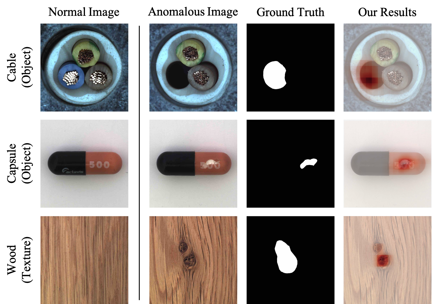
Figure 1: Image anomaly localization examples (from left to right): normal images, anomalous images, ground truth of the anomalous region and the predicted anomalous region by the proposed PEDENet, where the red region indicates the detected anomalous region. These examples are taken from the MVTec AD dataset.

Our work has the following three main contributions.

• We propose PEDENet for unsupervised image anomaly localization. It can be trained in an end-to-end manner with only normal images (i.e. unsupervised learning).

• Being inspired by the GMM, the DE network models the distribution of patch embeddings and computes the membership of a patch belonging to certain modalities. It helps find outlying artifact patches.

• Experiments show that PEDENet achieves state-of-the-art performance on unsupervised anomaly localization for the MVTec AD dataset.

The rest of this letter is organized as follows. Related previous work is reviewed in Sec. 2. The proposed PEDENet is presented in Sec. 3. Experimental results are shown in Sec. 4. Finally, concluding remarks are given in Sec. 5.

2 Related Work

Some related previous work is reviewed in this section. For image anomaly detection and localization, there are three commonly used approaches: 1) reconstruction-based, 2) pretrained network-based and 3) one-class classification-based approaches. They are reviewed in Secs. 2.1, 2.2 and 2.3, respectively. Finally, work on non-image anomaly data is briefly mentioned in Sec. 2.4.

2.1 Reconstruction-based Approach

Since normal samples are only available in training, the reconstruction-based approach utilizes the extraordinary capability of neural networks to focus on normal samples’ characteristics. Early work mainly uses the autoencoder and its variants [9, 10, 11, 12]. Since they are trained with only normal training data, it is unlikely for them to reconstruct abnormal images in the testing stage. As a result, the pixel-wise difference between the input abnormal image and its reconstructed image can indicate the region of abnormality. However, this approach is problematic due to inaccurate reconstructions or poorly calibrated likelihoods. More recently, several methods exploit factors on top of the reconstruction loss such as the incorporation of an attention map [13] or a student-teacher network to exploit intrinsic uncertainty in reconstruction [14]. A similar idea is to adopt the inpainting model as an alternative [15], [16]. It first removes part of an image and then reconstructs the missing part based on the visible part. The difference between the removed region and its inpainted result could tell the abnormality level of that region. Although they show promising results, the resolution of anomaly maps is somehow coarse due to the heavy computational burden.

2.2 Pretrained Network-based Approach

The performance of some computer vision algorithms can be improved by transfer learning using discriminative embeddings from pretrained networks. Along this line of thought, some models combine image features obtained by pretrained networks with anomaly detection algorithms. For example, the nearest-neighbor algorithm is used in [7] to examine whether an image patch of a test image is similar to any known normal image patches in the training set. The Gaussian distribution is adopted by [6] to fit the distribution of local features that are extracted from a pretrained network. However, since the pretrained networks are not specially optimized for the image anomaly detection task, the resulting model usually has a large model size.

2.3 One-class Classification-based Approach

Another natural idea is to adopt the Support Vector Data Description (SVDD) classifier. SVDD is a classic one-class classification algorithm derived from the Support Vector Machine (SVM). It maps all normal training data into a kernel space and seeks the smallest hypersphere that encloses the data in the space. Anomalies are expected to be located outside the learned hypersphere. Ruff et al. [17] first incorporated this idea in a deep neural network for non-image data anomaly detection and then extended it to an unsupervised setting [18]. They used a neural network to mimic the kernel function and trained it with the radius of the hypersphere. This modification allows an encoder to learn a data-dependent transformation, thus enhancing detection performance on high-dimensional and structured data. Later, Liznerski et al. [19] generalized it to image anomaly detection by applying a SVDD-inspired pseudo-Huber loss to the output matrix of a Fully Convolutional Network (FCN). It offers further improvements in a semi-supervised setting.

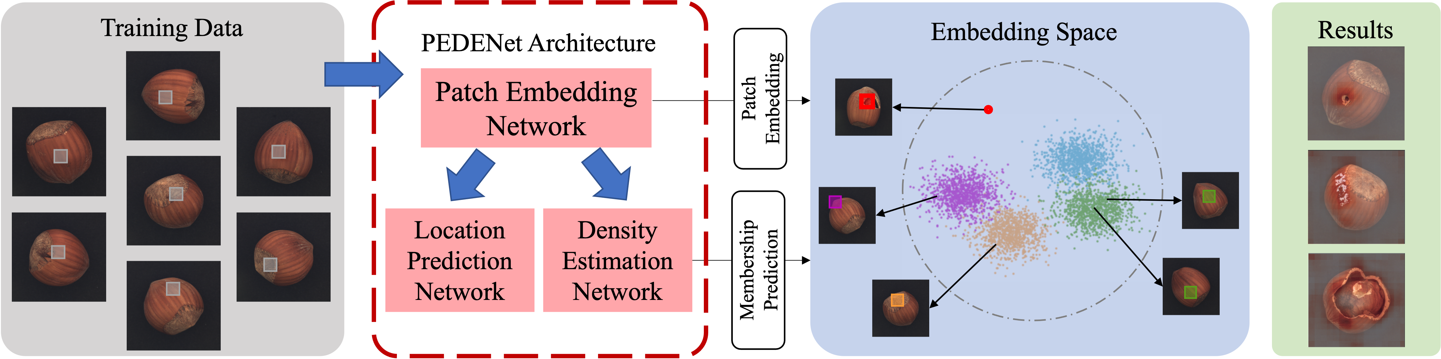
Figure 2: An overview of the proposed PEDENet. Image are first divided into patches and, then, fed into the Patch Embedding (PE) network for patch embeddings. The Density Estimation (DE) network conducts clustering in the embedding space. After training, normal patches are clustered, and outliers could be treated as abnormal patches in the inference stage. Three anomaly localization results from thee Hazelnut class are shown as examples.

2.4 Non-image Data

For anomaly detection on non-image data, a Deep Autoencoding Gaussian Mixture Model(DAGMM) was proposed in [20]. It combines dimensionality reduction and density estimation for unsupervised anomaly detection. Our proposed PEDENet is different from DAGMM in three aspects. First, PEDENet is designed for image anomaly localization while DAGMM targets at identifying an anomalous entity. Second, DAGMM employs an autoencoder (AE) to reconstruct the input data and concatenates latent features with reconstruction errors for density estimation. PEDENet adopts a PE network to learn local features and then applies the DE network to patch embeddings. Third, DAGMM demonstrates its performance on non-image data whose dimension is relatively lower. For example, the dimension of the latent space can be as low as one. In contrast, the dimension of patch embedding features is significantly higher in PEDENet.

3 Proposed Method

3.1 PEDENet

An overview of the PEDENet is shown in Fig. 2, where the Hazelnut class from the MVTec AD dataset is used as an illustrative input. PEDENet conducts class-specific training and testing. It contains a patch embedding (PE) network, a density estimation (DE) network, and an auxiliary network called the location prediction (LP) network. The PE network takes an image patch as its input and performs dimension reduction to get low-dimensional patch embeddings via a deep encoder structure. The DE network takes a patch embedding as the input and predicts its cluster membership under the framework of the Gaussian Mixture Model (GMM). These two networks are shown in Fig. 2. The LP network is a multi-layer perception (MLP). It takes a pair of patch embeddings as the input and predicts the relative location of them as depicted in Fig. 3.

PE Network. With an image patch as the input, the PE network outputs its low-dimensional embedding. Inspired by [21], we adopt a hierarchical encoder that embodies a larger encoder with several smaller encoders. That is, we divide an input patch, $p$, into $2\times 2$ sub-patches and feed each of smaller sub-patches into a smaller encoder. The outputs of the smaller sub-patches are aggregated based on their original positions. Then, they are encoded by a larger encoder to get the embedding of patch $p$. The above process can be summarized as

$$\bm{z}=\mbox{PEN}(\bm{p};\bm{\theta}_{PEN}),$$ (1)

where PEN denotes the PE network and $\bm{z}\in\mathbb{R}^{Z}$ is the low-dimensional embedding output of $p$, and $Z$ is the dimensionality of the embedding space. The PE network is implemented as a composite mapping consisting of smaller encoders, a larger encoder and the aggregation process with learnable parameters $\bm{\theta}_{PEN}$ as shown in the right-hand-side of Eq. (1).

DE Network. Given the low-dimensional embedding of an input patch, the DE network predicts its cluster membership values with respect to multiple Gaussian modalities under the Gaussian Mixture Model (GMM). A GMM assumes data samples are generated from a finite number of Gaussian distributions with unknown parameters. The Expectation-Maximization (EM) algorithm can be used to optimize those parameters iteratively. In the EM algorithm, the Expectation step computes the posterior probability (i.e. the so-called cluster membership) of each sample while the Maximization step updates the GMM parameters, including the mean vector, the covariance matrix and the mixture coefficient of each Gaussian component.

Note that GMM may suffer from a sub-optimal solution. Furthermore, it is challenging to combine it with a neural network to achieve end-to-end learning. By following the idea in DAGMM [20], we propose the DE network to estimate the cluster membership for each patch embedding, which corresponds to the expectation step of the EM algorithm:

$$\bm{\gamma}=\mbox{softmax}(\mbox{DEN}(\bm{z};\bm{\theta}_{DEN})),$$ (2)

where DEN indicates the DE network, $\bm{z}$ is the low-dimensional embedding generated by the PE network, and $\bm{\theta}_{DEN}$ denotes parameters of the DE network. After the softmax normalization, $\bm{\gamma}$ is a vector in $\mathbb{R}^{K}$, where $K$ is a hyper-parameter representing the number of Gaussian components in the GMM.

After getting the membership prediction $\bm{\gamma}$, we update GMM parameters. This corresponds to the maximization step of the EM algorithm. Here, we use $\phi_{k}$, $\bm{\mu_{k}}$ and $\bm{\Sigma}_{k}$ to represent the mixture coefficient, the mean vector, the covariance matrix of the $k$-th component, $1\leq k\leq K$. For a batch of $N$ patch embeddings, we have

$$\phi_{k} = \sum^{N}_{i=1}\frac{\gamma_{ik}}{N}\in\mathbb{R},$$ (3)

$$\bm{\mu_{k}} = \frac{\sum^{N}_{i=1}\gamma_{ik}\bm{z_{i}}}{\sum^{N}_{i=1}\gamma_{ik}}\in\mathbb{R}^{Z},$$ (4)

$$\bm{\sigma}_{k} = \frac{\sum^{N}_{i=1}\gamma_{ik}(\bm{z_{i}}-\bm{\mu_{k}})(\bm{z_{i}}-\bm{\mu_{k}})^{T}}{\sum^{N}_{i=1}\gamma_{ik}}\in\mathbb{R}^{Z\times Z}.$$ (5)

Then, we can express the probability of a patch embedding $\bm{z_{i}}$ in form of

$$P(\bm{z_{i}})=\sum^{K}_{k=1}\phi_{k}\frac{\exp(-\frac{1}{2}(\bm{z_{i}}-\bm{\mu_{k}})\bm{\Sigma}_{k}^{-1}(\bm{z_{i}}-\bm{\mu_{k}})^{T})}{\sqrt{2\pi|\bm{\Sigma}_{k}}|}\in[0,1],$$ (6)

where $|\cdot|$ means the determinant of a matrix. If a patch embedding, $\bm{z_{i}}$, has a large probability, it means the corresponding patch is likely to be a normal patch, and vice versa.

LP Network. Inspired by Patch-SVDD [21], we employee the LP network as an auxiliary network that predicts the relative location of two neighboring patches in a self-supervised manner. For an arbitrary input patch, $\bm{p}$, we sample another patch $\bm{p}^{\prime}$ from one of its eight neighbors as shown in Fig. 3. We feed patches $\bm{p}$ and $\bm{p}^{\prime}$ into the PE network to get their patch embeddings, $\bm{z}$ and $\bm{z}^{\prime}$, respectively. The relative location of patch $\bm{p}^{\prime}$ against patch $\bm{p}$ is encoded to a one-hot vector $\bm{l}\in\mathbb{R}^{8}$, used as the label in the training as:

$$\bm{\hat{l}}=\mbox{LPN}(\bm{z},\bm{z}^{\prime};\bm{\theta}_{LPN}),$$ (7)

where LPN denotes the LP network and $\bm{\theta}_{LPN}$ denotes its network parameters.

3.2 Loss Function

We propose the following loss function to train the PE, DE and LP networks jointly:

$$\mathcal{L}=\lambda_{1}\mathcal{L}_{DEN}+\lambda_{2}\mathcal{L}_{LPN}+\lambda_{3}\mathcal{L}_{reg},$$ (8)

where $\lambda_{1}$, $\lambda_{2}$, and $\lambda_{3}$ are parameters adjustable by users to assign a different weight to each loss terms. The three terms in the right of Eq. (8) are elaborated below.

The first loss term is needed for the DE network. Since the total probability, $P(\bm{z_{i}})$, models the likelihood of observing $\bm{z_{i}}$ as a normal patch. By maximizing the average total probability of input patches,

$$\mathcal{L}_{DEN}=-\frac{1}{N}\log\sum^{N}_{i=1}P(\bm{z_{i}}),$$ (9)

the DE network is trained to describe the distribution of patches embedding with an implicit GMM while the PE network can be optimized simultaneously. The second loss term is the cross-entropy loss between $l$ and $\hat{l}$ for the LP network as given in Eq. (9):

$$\mathcal{L}_{LPN}=-\sum^{8}_{i=1}l_{i}\cdot log(\hat{l_{i}}).$$ (10)

Finally, we add a regularization term to prevent singularity in the GMM, which occurs when the determinant of any $\bm{\Sigma}_{k}$ degenerates to zero. We add the regularization loss term to penalize small values of diagonal elements:

$$\mathcal{L}_{reg}=\sum^{K}_{k=1}\sum^{Z}_{z=1}\frac{1}{\bm{\Sigma}_{kz}}.$$ (11)

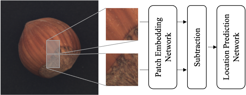
Figure 3: The diagram of the location prediction (LP) network.

End-to-end Training. With the total loss function given in Eq. (8), all three networks could be jointly optimized using the back-propagation algorithm. The DE network and the LP network are two parallel branches concatenated to the PE network. That is, the output of the PE network, i.e. patch embedding, serves as the input to the DE and the LP networks. The DE network takes a patch embedding directly. The LP network takes the difference of embeddings of a pair of adjacent patches and use their relative position as the training label. In the training, parameters of all three networks are updated simultaneously so as to achieve end-to-end training for the whole PEDENet.

3.3 Anomaly Localization

We obtain low-dimensional patch embeddings from the PE network so as to localize anomalies. Low-dimensional patch embeddings can be integrated with various anomaly detection models such as one-class SVM [22] and SVDD [23]. In this work, to illustrate the effectiveness of learned low-dimensional patch embeddings, we adopt the nearest neighbor rule in the embedding space to localize anomalous pixels. This was also used in [7, 21].

For every patch $p$ with stride $S$ in test image $X$, we use its $L_{2}$ distance to the nearest normal patch in the embedding space to define its anomaly score:

$$AS(\bm{p})=\min\ L_{2}(\bm{p},\bm{p}_{Normal}).$$ (12)

The pixel-wise anomaly score can be calculated by averaging anomaly scores of all patches to which this pixel belongs to. An approximate algorithm is adopted to mitigate the computational cost of the nearest neighbor search. The maximum anomaly score of pixels in an image is set to the image-level anomaly score.

Table 1: Comparison of image anomaly localization performance, where the evaluation metric is pixel-wise AUC-ROC. The best and the second best results are shown in bold face and with an underline, respectively.

AE L2 AE SSIM AnoGAN VAE SPADE Patch-SVDD FCDD PEDENet (ours) Bottle 0.86 0.93 0.86 0.831 0.984 0.981 0.80 0.984 Cable 0.86 0.82 0.78 0.831 0.972 0.968 0.80 0.971 Capsule 0.88 0.94 0.84 0.817 0.990 0.958 0.88 0.943 Hazelnut 0.95 0.97 0.87 0.877 0.991 0.975 0.96 0.970 Metal 0.86 0.89 0.76 0.787 0.981 0.980 0.88 0.973 Pill 0.85 0.91 0.87 0.813 0.965 0.951 0.86 0.960 Screw 0.96 0.96 0.80 0.753 0.989 0.957 0.87 0.972 Teeth brush 0.93 0.92 0.90 0.919 0.979 0.981 0.90 0.979 Transistor 0.86 0.90 0.80 0.754 0.941 0.970 0.80 0.982 Zipper 0.77 0.88 0.78 0.716 0.965 0.951 0.81 0.962 All 10 Object Classes 0.88 0.91 0.83 0.810 0.976 0.967 0.86 0.970 Carpet 0.59 0.87 0.54 0.597 0.975 0.926 0.93 0.922 Grid 0.90 0.94 0.58 0.612 0.937 0.962 0.87 0.959 Leather 0.75 0.78 0.64 0.671 0.976 0.974 0.98 0.976 Tile 0.51 0.59 0.50 0.513 0.874 0.914 0.92 0.926 Wood 0.73 0.73 0.62 0.666 0.885 0.908 0.89 0.900 All 5 Texture Classes 0.70 0.78 0.29 0.612 0.929 0.937 0.92 0.936 Average of 15 Classes 0.82 0.87 0.74 0.744 0.965 0.957 0.88 0.959

Table 2: Comparison of image anomaly detection performance, where the evaluation metric is the image-level AUC-ROC. The best and the second best results are shown in bold face and with an underline, respectively.

	GANomaly	ITAE	Patch-SVDD	SPADE	MahalanobisAD	PEDENet (ours)
Image-Level AUC-ROC	0.762	0.839	0.921	0.855	0.958	0.928

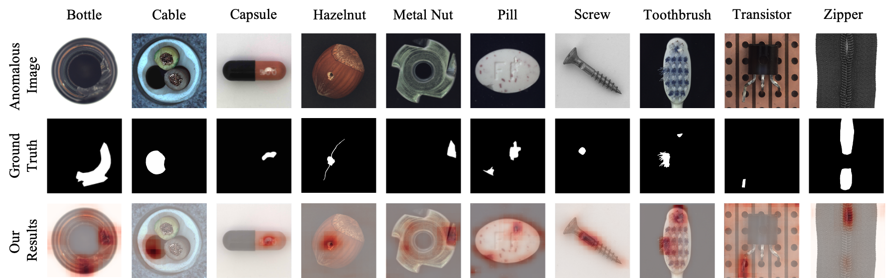
Figure 4: Visualization of anomalous images, labeled ground truths and localization results of the proposed PEDENet for 10 object classes in the MVTec AD dataset, where the red color is used to indicate detected anomaly regions.

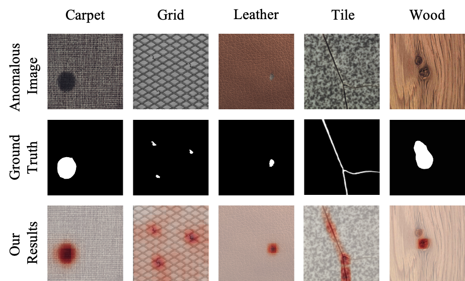
Figure 5: Visualization of anomalous images, labeled ground truths and localization results of the proposed PEDENet for 5 texture classes in the MVTec AD dataset, where the red color is used to indicate detected anomaly regions.

4 Experiments

4.1 Experimental Setup

To verify the effectiveness of the proposed PEDENet, we conducted experiments on the MVTec AD dataset [24], which is a comprehensive anomaly localization dataset collected from real world scenarios. It consists of images belonging to 15 classes, including 10 object classes and 5 texture classes. For each class, there are 60-391 training images and 40-167 test images, where image sizes varies from $700\times 700$ to $1024\times 1024$. The training set contains only normal images while the test set contains both normal and anomalous images. Examples of normal and anomalous images are shown in Fig. 1. We train and evaluate anomaly localization algorithms for each class separately, which is known as class-specific evaluation. To train a model, all training images are first resized to $256\times 256$ and, then, patches of size $64\times 64$ are randomly sampled from these resized images.

Our proposed solution consists of three networks: 1) the PE network, 2) the DE network, and 3) the LP network. The PE network consists of eight convolutional layers and one output layer. The filter size in all convolutional layers is the same, i.e. $3\times 3$. The filter numbers for convolutional layers are 32, 64, 128, 128, 64, 64, 32, 32, 64 and LeakyReLU [25] with slope 0.1 is used as activation function. The tanh activation is used in the output layer to normalize the output to the range of [-1.0,1.0]. Both the DE and LP networks are multilayer perceptrons (MLPs) with the LeakyReLU activation of slope 0.1. The DE network has three hidden layers of 128, 64, 32 neurons, respectively. The LP network has two hidden layers of 128 neurons per layer. The input to the LP network is subtraction of features from two neighboring patches.

We train all networks using the Adam optimizer with learning rate 0.0001. The batch sizes are 128 image patches for the DE network and 36 pairs of adjacent patches for the LP network. All experiments are conducted on a machine equipped with an Intel i7-5930K CPU and an NVIDIA GeForce Titan X GPU.

4.2 Performance Evaluation

Anomaly Localization. We compare the image anomaly localization performance of several methods with respect to the MVTec AD dataset [24] in Table 1, where the evaluation metric is the pixel-wise area under the receiver operating characteristic curve (AUC-ROC). The benchmarking methods are listed below.

• Reconstruction approach: AE L2 [24], AE SSIM [9], Variational Autoencoder(VAE) and AnoGAN [2].

• Pre-trained network based approach: SPADE [7].

• One-class classification approach: Patch-SVDD[21], and FCDD [19].

Our proposed PEDENet achieves 97.0% for the average of 10 object classes (the 2nd best), 93.6% for the average of 5 texture classes (the 2nd best), and 95.9% for the average of all 15 classes (the 2nd best). Note that there is no single method that performs the best in all cases. PEDENet is second to SPADE in the average of 10 object classes while it is second to Patch-SVDD in the average of the 5 texture classes. The performance differences among SPADE, Patch-SVDD and PEDENet are actually quite small. Thus, it is fair to say that PEDENet is one of the state-of-the-art methods for image anomaly localization.

Anomaly Detection. We compare image anomaly detection performance in Table 2, where the evaluation metric is the image-level area under the receiver operating characteristic curve (AUC-ROC). The benchmarking methods include: GANomaly [26], ITAE [27], Patch-SVDD [21], SPADE [7] and MahalanobisAD [6]. Our proposed PEDENnet reaches 92.8%. It outperforms both SPADE and Patch-SVDD. It is only second to MahalanobisAD. Thus, PEDENnet also offers state-of-the-art image anomaly detection performance.

Visualization of Localized Anomalies. Anomalous images, labeled ground truths and localization results of the proposed PEDENet for 10 object classes and 5 texture classes in the MVTec AD dataset are visualized in Figs. 4 and 5, respectively. Anomalous regions are highlighted in red. A region is more likely to be anomalous if it has stronger red color. As shown in those figures, anomalous regions could be accurately detected and localized by the proposed PEDENet. Note that relatively small and inconspicuous defects can still be spotted such as Capsule, Hazelnut and Pill examples in Fig. 4.

Model Size. Most state-of-the-art methods that give the best performance take the pre-trained network approach such as SPADE [7], and MahalanobisAD [6]. As a result, their model sizes are usually quite large. We compare the model sizes of these three methods in Table 3 in terms of the number of model parameters. The numbers of model parameters of SPADE and MahalanobisAD are 145$\times$ and 36$\times$ of that of PEDENet. A smaller model size means lower memory requirement which is critical in real-world deployment. Besides being a light-weighted network, PEDENet is trained using the training data in the MVTec AD dataset only. In contrast, the two benchmarking methods leverage giant models that are pre-trained by millions of labeled images.

Table 3: Model Size Comparison

Methods	Pre-trained Model	# of Parameters
SPADE	Wide ResNet-50	68M
MahalanobisAD	EfficientNet-B4	17M
PEDENet (ours)	None	0.47M

Table 4: Ablation Study

$\mathcal{L}_{DEN}$	$\mathcal{L}_{LPN}$	AUC-ROC
$\surd$		0.810
	$\surd$	0.894
$\surd$	$\surd$	0.959

Ablation Study. We conduct ablation study to understand the impact of each loss term in Eq. (8) to the performance of the proposed PEDENet. That is, we remove either $\mathcal{L}_{DEN}$ or $\mathcal{L}_{LPN}$ and train the model under the same condition. We see from Table 4 that the adoption of both $\mathcal{L}_{DEN}$ and $\mathcal{L}_{DEN}$ as shown in Eq. (8) improves the anomaly localization performance.

Challenge of Texture Classes. It is worthwhile to point out that almost all methods have an obvious performance gap between the object classes and the texture classes. As shown in Table 1, the performance gap varies from $3\%$ [21] to almost $20\%$ [9]. As mentioned in [21], the optimal hyper-parameters for objects and textures are likely to be different and there is a trade-off to get the best average performance. Actually, texture and regular images are treated differently in image processing. There many unique methods developed specifically for textures [28, 29, 30, 31]. Unlike regular images, there are strong self-similarity and quasi-periodicity in textures, which could be exploited to achieve further performance improvement.

5 Conclusion and Future Work

A new neural network model, called the PEDENet, was proposed for image anomaly detection and localization. It is a lightweight model and offers state-of-the-art anomaly detection and localization performance. There are some future research topics. First, the MVTec AD dataset is still too small. It is valuable to collect more samples and build a larger dataset. Second, it is desired to find a more effective solution for texture anomaly detection and localization. Third, there are many hyper-parameters in the proposed PEDENnet, which are finetuned by trial and error. A more systematic approach is needed. Finally, it is interesting to find an altenative image anomaly detection and localization solution that is effective and interpretable.

References

- [1] Luke Scime and Jack Beuth. Anomaly detection and classification in a laser powder bed additive manufacturing process using a trained computer vision algorithm. Additive Manufacturing, 19:114–126, 2018.
- [2] Thomas Schlegl, Philipp Seeböck, Sebastian M Waldstein, Ursula Schmidt-Erfurth, and Georg Langs. Unsupervised anomaly detection with generative adversarial networks to guide marker discovery. In International conference on information processing in medical imaging, pages 146–157. Springer, 2017.
- [3] Thomas Schlegl, Philipp Seeböck, Sebastian M Waldstein, Georg Langs, and Ursula Schmidt-Erfurth. f-anogan: Fast unsupervised anomaly detection with generative adversarial networks. Medical image analysis, 54:30–44, 2019.
- [4] Venkatesh Saligrama and Zhu Chen. Video anomaly detection based on local statistical aggregates. In 2012 IEEE Conference on Computer Vision and Pattern Recognition, pages 2112–2119. IEEE, 2012.
- [5] Joey Tianyi Zhou, Jiawei Du, Hongyuan Zhu, Xi Peng, Yong Liu, and Rick Siow Mong Goh. Anomalynet: An anomaly detection network for video surveillance. IEEE Transactions on Information Forensics and Security, 14(10):2537–2550, 2019.
- [6] Oliver Rippel, Patrick Mertens, and Dorit Merhof. Modeling the distribution of normal data in pre-trained deep features for anomaly detection. arXiv preprint arXiv:2005.14140, 2020.
- [7] Niv Cohen and Yedid Hoshen. Sub-image anomaly detection with deep pyramid correspondences. arXiv preprint arXiv:2005.02357, 2020.
- [8] Kaitai Zhang, Bin Wang, Wei Wang, Fahad Sohrab, Moncef Gabbouj, and C-C Jay Kuo. Anomalyhop: An ssl-based image anomaly localization method. IEEE Visual Communications and Image Processing (VCIP), 2021.
- [9] Paul Bergmann, Sindy Löwe, Michael Fauser, David Sattlegger, and Carsten Steger. Improving unsupervised defect segmentation by applying structural similarity to autoencoders. In Alain Trémeau, Giovanni Maria Farinella, and José Braz, editors, Proceedings of the 14th International Joint Conference on Computer Vision, Imaging and Computer Graphics Theory and Applications, VISIGRAPP 2019, Volume 5: VISAPP, Prague, Czech Republic, February 25-27, 2019, pages 372–380. SciTePress, 2019.
- [10] Mohammadreza Salehi, Ainaz Eftekhar, Niousha Sadjadi, Mohammad Hossein Rohban, and Hamid R Rabiee. Puzzle-ae: Novelty detection in images through solving puzzles. arXiv preprint arXiv:2008.12959, 2020.
- [11] Wenqian Liu, Runze Li, Meng Zheng, Srikrishna Karanam, Ziyan Wu, Bir Bhanu, Richard J Radke, and Octavia Camps. Towards visually explaining variational autoencoders. In Proceedings of the IEEE/CVF Conference on Computer Vision and Pattern Recognition, pages 8642–8651, 2020.
- [12] Marco Rudolph, Bastian Wandt, and Bodo Rosenhahn. Same same but differnet: Semi-supervised defect detection with normalizing flows. In Proceedings of the IEEE/CVF Winter Conference on Applications of Computer Vision, pages 1907–1916, 2021.
- [13] Shashanka Venkataramanan, Kuan-Chuan Peng, Rajat Vikram Singh, and Abhijit Mahalanobis. Attention guided anomaly localization in images. In European Conference on Computer Vision, pages 485–503. Springer, 2020.
- [14] Paul Bergmann, Michael Fauser, David Sattlegger, and Carsten Steger. Uninformed students: Student-teacher anomaly detection with discriminative latent embeddings. In Proceedings of the IEEE/CVF Conference on Computer Vision and Pattern Recognition, pages 4183–4192, 2020.
- [15] Zhenyu Li, Ning Li, Kaitao Jiang, Zhiheng Ma, Xing Wei, Xiaopeng Hong, and Yihong Gong. Superpixel masking and inpainting for self-supervised anomaly detection. In 31st British Machine Vision Conference, pages 7–10, 2020.
- [16] Vitjan Zavrtanik, Matej Kristan, and Danijel Skočaj. Reconstruction by inpainting for visual anomaly detection. Pattern Recognition, 112:107706, 2021.
- [17] Lukas Ruff, Robert Vandermeulen, Nico Goernitz, Lucas Deecke, Shoaib Ahmed Siddiqui, Alexander Binder, Emmanuel Müller, and Marius Kloft. Deep one-class classification. In International conference on machine learning, pages 4393–4402. PMLR, 2018.
- [18] Lukas Ruff, Robert A Vandermeulen, Nico Görnitz, Alexander Binder, Emmanuel Müller, Klaus-Robert Müller, and Marius Kloft. Deep semi-supervised anomaly detection. arXiv preprint arXiv:1906.02694, 2019.
- [19] Philipp Liznerski, Lukas Ruff, Robert A Vandermeulen, Billy Joe Franks, Marius Kloft, and Klaus-Robert Müller. Explainable deep one-class classification. arXiv preprint arXiv:2007.01760, 2020.
- [20] Bo Zong, Qi Song, Martin Renqiang Min, Wei Cheng, Cristian Lumezanu, Daeki Cho, and Haifeng Chen. Deep autoencoding gaussian mixture model for unsupervised anomaly detection. In International Conference on Learning Representations, 2018.
- [21] Jihun Yi and Sungroh Yoon. Patch-SVDD: Patch-level SVDD for anomaly detection and segmentation. In Proceedings of the Asian Conference on Computer Vision, 2020.
- [22] Yunqiang Chen, Xiang Sean Zhou, and Thomas S Huang. One-class svm for learning in image retrieval. In Proceedings 2001 International Conference on Image Processing (Cat. No. 01CH37205), volume 1, pages 34–37. IEEE, 2001.
- [23] David MJ Tax and Robert PW Duin. Support vector data description. Machine learning, 54(1):45–66, 2004.
- [24] Paul Bergmann, Michael Fauser, David Sattlegger, and Carsten Steger. MVTec AD–A comprehensive real-world dataset for unsupervised anomaly detection. In Proceedings of the IEEE/CVF Conference on Computer Vision and Pattern Recognition, pages 9592–9600, 2019.
- [25] Kaiming He, Xiangyu Zhang, Shaoqing Ren, and Jian Sun. Delving deep into rectifiers: Surpassing human-level performance on imagenet classification. In Proceedings of the IEEE international conference on computer vision, pages 1026–1034, 2015.
- [26] Samet Akcay, Amir Atapour-Abarghouei, and Toby P Breckon. Ganomaly: Semi-supervised anomaly detection via adversarial training. In Asian conference on computer vision, pages 622–637. Springer, 2018.
- [27] Ye Fei, Chaoqin Huang, Cao Jinkun, Maosen Li, Ya Zhang, and Cewu Lu. Attribute restoration framework for anomaly detection. IEEE Transactions on Multimedia, 2020.
- [28] Tianhorng Chang and C-CJ Kuo. Texture analysis and classification with tree-structured wavelet transform. IEEE Transactions on image processing, 2(4):429–441, 1993.
- [29] Kaitai Zhang, Hong-Shuo Chen, Ye Wang, Xiangyang Ji, and C.-C. Jay Kuo. Texture analysis via hierarchical spatial-spectral correlation (HSSC). In 2019 IEEE International Conference on Image Processing (ICIP), pages 4419–4423. IEEE, 2019.
- [30] Kaitai Zhang, Hong-Shuo Chen, Xinfeng Zhang, Ye Wang, and C.-C. Jay Kuo. A data-centric approach to unsupervised texture segmentation using principle representative patterns. In ICASSP 2019-2019 IEEE International Conference on Acoustics, Speech and Signal Processing (ICASSP), pages 1912–1916. IEEE, 2019.
- [31] Kaitai Zhang, Bin Wang, Hong-Shuo Chen, Ye Wang, Shiyu Mou, and C.-C. Jay Kuo. Dynamic texture synthesis by incorporating long-range spatial and temporal correlations. arXiv preprint arXiv:2104.05940, 2021.