figurec
On Label Shift in Domain Adaptation
via Wasserstein Distance
| Trung Le‡ | Dat Do§ | Tuan Nguyen‡ | Huy Nguyen⋄ |
| Hung Bui⋄ | Nhat Ho† | Dinh Phung‡ |
| Monash University‡; VinAI Research⋄; |
| University of Michigan, Ann Arbor§; University of Texas, Austin† |
Abstract
We study the label shift problem between the source and target domains in general domain adaptation (DA) settings. We consider transformations transporting the target to source domains, which enable us to align the source and target examples. Through those transformations, we define the label shift between two domains via optimal transport and develop theory to investigate the properties of DA under various DA settings (e.g., closed-set, partial-set, open-set, and universal settings). Inspired from the developed theory, we propose Label and Data Shift Reduction via Optimal Transport (LDROT) which can mitigate the data and label shifts simultaneously. Finally, we conduct comprehensive experiments to verify our theoretical findings and compare LDROT with state-of-the-art baselines.
1 Introduction
The remarkable success of deep learning can be largely attributed to computational power advancement and large-scale annotated datasets. However, in many real-world applications such as medicine and autonomous driving, labeling a sufficient amount of high-quality data to train accurate deep models is often prohibitively labor-expensive, error-prone, and time-consuming. Domain adaptation (DA) or transfer learning has emerged as a vital solution for this issue by transferring knowledge from a label-rich domain (a.k.a. source domain) to a label-scarce domain (a.k.a. target domain). Along with practical DA methods [14, 43, 32, 40, 13] which have achieved impressive performance on real-world datasets, the theoretical results [34, 3, 38, 50, 8] are abundant to provide rigorous and insightful understanding of various aspects of transfer learning.
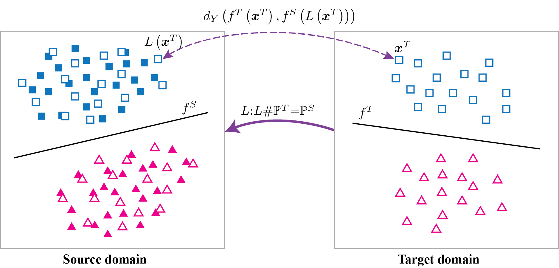
For domain adaptation, the source domain consists of the data distribution with the density , and the unknown ground-truth labeling function assigning label to source data , whilst these are , , and for the target domain, respectively. Moreover, while the data shift can be characterized as a divergence between and [34, 3, 38, 50, 8], the label shift in these works is commonly characterized as or in which the binary classification with deterministic labeling functions was examined. Additionally, although this label shift term has occurred in the theoretical analysis of [34, 3, 38, 50, 8], it is restricted in considering the shift between and at the same data , which ignores the data shift between and . This limitation is illustrated in Figure 1. In particular, for a white/square point drawn from the target domain as in , the source labeling function cannot give reasonable prediction probabilities for , hence leading to inaccurate .
Label shift has also been examined in an anti-causal setting [31, 16], wherein an intervention on induces the shift, but the process generating given is fixed, i.e., . Although this setting is useful in some specific scenarios (e.g., a diagnostic problem in which diseases cause symptoms), it is not sufficiently powerful to cope with a general DA setting. Particularly, in an anti-causal setting, the source and target data distributions (i.e., and ) are just simply two different mixtures of the class conditional distributions , hence sharing the same support set. This is certainly far from a general DA setting in which both data shift: with arbitrarily separated support sets and non-covariate shift: appear.
Contribution. In this paper, we study the label shift for a general domain adaptation setting in which we have both data shift: with arbitrarily separated support sets and non-covariate shift: . More specifically, our developed label shift is applicable to a general DA setting with a data shift between two domains and two totally different labeling functions (i.e., we cannot use to predict accurately target examples and vice versa). To define the label shift between two given domains, we utilize transformation to transport the target to the source data distributions (i.e., ). This transformation allows us to align the data of two domains. Subsequently, the label shift between two domains is defined as the infimum of the label shift induced by such a transformation with respect to all feasible transformations. This viewpoint of label shift has a connection to optimal transport [39, 46, 37], which enables us to develop theory to quantify the label shift for various DA settings, e.g., anti-causal, closed-set, partial-set, open-set, and universal settings. Overall, our contributions can be summarized as follows:
1. We characterize the label shift for a general DA setting via optimal transport. From that, we develop a theory to estimate the label shift for various DA settings and study the trade-off of learning domain-invariant representations and WS label shift.
2. Inspired from the theoretical development, we propose Label and Data Shift Reductions via Optimal Transport (LDROT) which aims to mitigate both data and label shifts. We conduct comprehensive experiments to verify our theoretical findings and compare the proposed LDROT with the baselines to demonstrate the favorable performance of our method.
Related works. Several attempts have been proposed to characterize the gap between general losses of source and target domains in DA, notably [34, 3, 38, 50, 8]. [5, 4, 50] study the impossibility theorems for DA, attempting to characterize the conditions under which it is nearly impossible to perform transferability between domains. PAC-Bayesian view on DA using weighted majority vote learning has been rigorously studied in [19, 20]. Meanwhile, [52, 23] interestingly indicate the insufficiency of learning domain-invariant representation for successful adaptation. Specifically, [52] points out the degradation in target predictive performance if forcing domain invariant representations to be learned while two marginal label distributions of the source and target domains are overly divergent. [23] analyzes the information loss of non-invertible transformations and proposes a generalization upper bound that directly takes it into account. [25] employed a transformation to align two domains and developed theories based on this assumption. Moreover, label shift has been examined for the anti-causal setting [31, 16], which seems not sufficiently realistic for a general DA setting. Optimal transport theory has been theoretically leveraged with domain adaptation [9]. We compare our proposed LDROT to DeepJDOT [10] (a deep DA approach based on the theory of [9]), and other OT-based DDA approaches, including SWD [26], DASPOT [47], ETD [27], RWOT [49]. Finally, in [42] , a generator is said to produce generalized label shift (GLS) representations if it transports source class conditional distributions to corresponding target ones. Further theories were developed to indicate that GLR representations are satisfied if we enforce clustering structure assumption assisting us in training a perfect classifier. Evidently, our work which focuses on how to quantify the label shift between two different domains taking into account the inherent data shift via optimal transport theory is totally different form that work in terms of motivation and developed theory.
2 Label Shift with Wasserstein Distance
2.1 Preliminaries
Notation. For a positive integer and a real number , indicates the set while denotes the -norm of a vector . Let and be the label sets of the source and target domains that have and elements, respectively. Meanwhile, stands for the label set of both domains which has the cardinality of . Subsequently, we denote , , and as the simplices corresponding to , and respectively. Finally, let and be the labeling functions of the source and target domains, respectively, by filling zeros for the missing labels.
We now examine a general supervised learning setting. Consider a hypothesis in a hypothesis class and a labeling function where . Let be a metric over , we further define a general loss of the hypothesis with respect to the labeling function and the data distribution as: .
Next, we consider a domain adaptation setting in which we have source space endowed with a distribution and the density function , and a target space endowed with a distribution and the density function . We examine various DA settings based on the labels of source and target domains including (1) closed-set DA: , (2) open-set DA: , (3) partial-set DA: , and (4) universal DA: and .
2.2 Background on label shift
Together with data shift, the study of label shift is important for a general DA problem. However, due to the occurrence of data shift, it is challenging to formulate label shift in a general DA setting. Recent works [31, 16] have studied label shift for the anti-causal setting in which an intervention on induces the shift, but the process generating given is fixed, i.e., . In spite of being useful in some specific cases, the anti-causal setting is restricted and cannot represent data shift broadly because the source data distribution and the target data distribution are simply just two different mixtures of identical class conditional distributions. Furthermore, the label shift framework from these works is non-trivial to generalize to all settings of DA.
In this paper, we address the issues of the previous works by defining a novel label shift framework via Wasserstein (WS) distance for a general DA setting that takes into account the data shift between two domains. We then develop a theory for our proposed label shift based on useful properties of WS distance, such as its horizontal view, numeric stability, and continuity [2]. We refer readers to [39, 46, 37] for a comprehensive knowledge body of optimal transport theory and WS distance, and Appendix A for necessary backgrounds of WS for this work.
2.3 Label Shift via Wasserstein Distance
To facilitate our ensuing discussion, we assume that the source (S) and target (T) distributions and are atomless distributions on Polish spaces. Therefore, there exists a transformation such that [46]. Given that mapping , a data example with the ground-truth prediction probability corresponds to another data example with the ground-truth prediction probability . Hence, it induces a label mismatch loss
where is a given metric over . Based on that concept, the label shift between the source and target domains induced by the transformation can be defined as
| (1) |
By finding the optimal mapping , the label shift between two domains is defined as follows.
Definition 1.
Let be a metric over the simplex . The label shift between the source and the target domains is defined as the infimum of the label shift induced by all valid transformations :
| (2) |
We give an illustration for Definition 1 in Figure 1. The label shift in Eq. (2) suggests finding the optimal transformation to optimally align the source and target domains with a minimal label mismatch.
Properties of label shift via Wasserstein distance: To show the connection between the aforementioned label shift and optimal transport, we introduce two ways of calculating the label shift via Wasserstein distance.
Proposition 2.
(i) Denote by the joint distribution of , where , and the joint distribution of , where . Then, we have:
(ii) Let and be the push-forward measures of and via and respectively, i.e., and . Then, we have:
The results of Proposition 2 indicate that we can compute the label shift via the Wasserstein distance on the simplex. For example, when , the label shift can be computed via the familiar distance between and , i.e., . Note that with was studied in [9] for proposing a DA method that can mitigate both label and data shifts. However, the concept label shift was not characterized and defined explicitly in that work. Moreover, our motivation and theory development in this work are different and independent from [9].
In addition, [25] uses a transformation with the aim to reduce the data shift between the source and target domains. The variance of general losses of a source classifier when predicting on the source domain and that of the corresponding target classifier when predicting on the target domain is inspected, which introduces the label shift via this transformation (cf. Theorem 1 in that paper). However, the definition of the label shift is totally dependent on the transformation . It is worth noting that in this work, we do not consider an arbitrary transformation as in [25]. Instead, we look in and define the label shift as the infimum of the label shifts induced by valid transformations. To give a better understanding of our label shift definition, we now present some bounds for it in general and specific cases.
Proposition 3.
Denote by and the marginal distributions of the source and target domain labels, i.e., and . For when , the following holds:
(i) where the constant can be viewed as a reconstruction term: ;
(ii) ;
(iii) In the setting that and are mixtures of well-separated Gaussian distributions, i.e., with , in which denotes the operator norm and is sufficiently large, we have
| (3) |
where is a small constant depending on , and it goes to 0 as .
A few comments on Proposition 3 are in order. The inequality in (i) bounds the target loss by the source loss and the label shift. Though this inequality has the same form as those in [34, 3, 38, 50, 8], the label shift in our inequality is more reasonably expressed. The inequality in (ii) reads that the marginal label shift is a lower bound of our label shift. Therefore, the label shift induced by the best transformation can not be less than this quantity. A direct consequence is that implies , for all (no label shift). Finally, the inequality in (iii) shows that when the classes are well-separated, the label shift will almost achieve the lower bound in the first inequality, which implies its tightness. The key step in the proof is proving that and will be concentrated around the vertices and it is also provable for sub-Gaussian distributions with some extra work. The bound gives a simple way to estimate the label shift in this scenario: instead of measuring the Wasserstein distance on the simplex , we only need to measure the Wasserstein distance between the vertices equipped with the masses and . The first experiment in Section 4.1 also supports this finding.
Our label shift formulation can also serve as a tool to elaborate other aspects of DA, as we will see below.
Minimizing data shift while ignoring label shift can hurt the prediction on test set: Consider two classifiers on the source and target domains and where , are the source and target feature extractors, and with . We define a new metric with respect to the family as follows:
where and lie on the latent space . The necessary (also sufficient) condition under which is a proper metric on the latent space (see the proof in Appendix B) is realistic and not hard to be satisfied (e.g., the family contains any bijection). We now can define a Wasserstein distance that will be used in the development of Theorem 4.
Theorem 4.
With regard to the latent space , we can upper-bound the label shift as
Theorem 4 indicates a trade-off of learning domain-invariant representation by forcing (e.g., ). It is evident that if the label shift between domains is significant, because can be trained to be sufficiently small, learning domain-invariant representation by minimizing leads to a hurt in the performance of the target classifier on the target domain. Similar theoretical result was discovered in [52] for the binary classification (see Theorem 4.9 in that paper). However, our theory is developed based on our label shift formulation in a more general multi-class classification setting and uses WS distance rather than Jensen-Shannon (JS) distance [12] as in [52] for which the advantages of WS distance over JS distance have been thoughtfully discussed in [2].
Label shift under different settings of DA: An advantage of our method is that it can measure the label shift under various DA settings (i.e., open-set, partial-set, and universal DA). Doing this task is not straight-forward using other label shift methods. For example, if there is a label that appears in a domain but not in the other, it is not meaningful to measure the ratio between the marginal distribution of this label as in [17].
In what follows, we elaborate our label shift in those settings. Particularly, we provide some lower bounds for it, implying that the label shift is higher if there is label mismatch between two domains. Recall that when the source and target domains do not have the same number of labels, we can extend and to be functions taking values on by filling for the missing labels. For the sake of presenting the results, let be the common labels of two domains, the marginal of and the marginal of on the first dimensions. denotes the marginal of in the space of variables having labels and denotes the marginal of in the space of variables having labels .
Theorem 5.
Assume that . Then, the following holds:
i) For the partial-set setting (i.e., ), we obtain
| (4) |
ii) For the open-set setting (i.e., ), we obtain
| (5) |
iii) For the universal setting (i.e., and ), we have
| (6) |
Theorem 5 reveals that the label shifts for the partial-set, open-set, or universal DA settings are higher than the vanilla closed-set setting due to the missing and unmatching labels of two domains (see Section 4.1). Our theory also implicitly indicates that by setting appropriate weights for source and target examples (i.e., low weights for the examples with missing and unmatching labels), we can deduct label shift by reducing the second term of lower-bounds in Eqs. (4), (5), and (6) to mitigate the negative transfer [6]. We leave this interesting investigation to our future work. Moreover, further analysis can be found in Appendix C.
3 Label and Data Shift Reductions via Optimal Transport
3.1 Motivation theorem for our approach
We consider the source classifier and the target classifier . Given a decreasing function , a classifier is said to be -Lipschitz transferable [9] w.r.t a joint distribution , the metric on the data space, and the metric on the if for all , we have
Theorem 6.
Assume that , the target classifier is -Lipschitz transferable w.r.t the optimal joint distribution of with the metric on the data space and on the simplex , we have
| (7) |
where and the label shift is defined as
representing how accurate the target classifier imitates its ground-truth labeling function on the target domain.
Theorem 6 hints us how to devise our Label andData Shift Reductions via Optimal Transport (LDROT), aiming to reduce both data and label shifts simultaneously. First, we train the source classifier to work well on the source domain by minimizing . Second, we minimize the shifting loss to encourage to imitate . We will later explain how minimizing this shifting loss helps to reduce both data and label shifts simultaneously. Third, we encourage the target classifier to atisfy the Lipschitz condition or become smoother by making and as small as possible.
3.2 Objective function of LDROT
Our LDROT consists of three losses which are as follows:
(i) Standard loss : We train the source classifier on the labeled source data by minimizing the loss ;
(ii) Shifting loss : Furthermore, to mitigate both label and data shifts, we propose to further regularize the loss by , where the ground metric is defined as
| (8) |
where with and with ;
(iii) Clustering loss : Finally, to enhance the smoothness of , we enforce the clustering assumption [7] to enable giving the same prediction for source and target examples on the same cluster. To employ the clustering assumption [40], we use Virtual Adversarial Training (VAT) [35] in conjunction with minimizing the entropy of prediction [21]: with
where represents a Kullback-Leibler divergence, is a very small positive number, , and specifies the entropy.
Combining the above losses, we arrive at the following objective function of LDROT.
| (9) |
where . In addition, we use the target classifier to predict target examples.
Remark on the shifting term: We now explain why including the shifting term supports to reduce label and data shifts. First, we have the following inequality whose proof can be found in Appendix C:
| (10) |
since .
Therefore, by including the shifting term , we aim to reduce , which is useful for reducing the data shift on the latent space.
Second, we find that since . The inequality (i) in Proposition 3 suggests that reducing the label shift helps to reduces the loss on the target domain, therefore increasing the quality of our DA method. Finally, by including , we aim to simultaneously reduce both terms and , which is equal to . That step helps reduce the data shift between and , while forcing to mimic for predicting well on the target domain via reducing the label shift .
3.3 Training procedure of LDROT
We now discuss a few important aspects of the training procedure of LDROT.
Similarity-aware version of the ground metric : The weight in the ground metric in Eq. (8) represents the matching extent of and . Ideally, we would like to replace this fixed constant by varied weights in such a way that is high if and share the same label and low otherwise. However, it is not possible because the label of is unknown. As an alternative, it appears that if we can have a good way to estimate the pairwise similarity of and , seems to be high if and share the same label and low if otherwise. Based on this observation, we instead propose using a similarity-aware version of metric as follows:
where the weight is estimated based on .
Entropic regularized version of shifting term: Since computing directly the shifting term is expensive, we use the entropic regularized version of instead, which we denote where is a positive regularized term (Detailed definition and discussion of the entropic regularized Wasserstein metric is in Appendix A). The dual-form [18] of that entropic regularized term with respect to the ground metric admits the following form:
| (11) |
where is a neural net named the Kantorovich potential network, and are source and target data, , , and .
Evaluating the weights : The weights are evaluated based on the similarity scores . Basically, we train from scratch or fine-tune a pre-trained deep net (e.g., ResNet [22]) using source dataset with labels and compute cosine similarity of latent representations and of and as
To ease the computation, we estimate the weights according to source and target batches. Specifically, we consider a balanced source batch of source examples (i.e., is the number of classes and is source batch size for each class). For a target example in the target batch, we sort the similarity array in an ascending order. Ideally, we expect that the similarity scores of the target example and the source examples with the same class as (i.e., totally we have of theirs) are higher than other similarity scores in the current source batch. Therefore, we find as the -percentile of the ascending similarity array and compute the weights as with a temperature variable . It is worth noting that this weight evaluation strategy assists us in sharpening and contrasting the weights for the pairs in the similar and different classes. More specifically, for the pairs in the same classes, tend to be bigger than , whilst for the pairs in different classes, tend to be smaller than . Hence, with the support of exponential form and temperature variable , for the pairs in the same classes tend to be higher than those for the pairs in different classes. More specifically, for the pairs in the same classes, tend to be bigger than , whilst for the pairs in different classes, tend to be smaller than . Hence, with the support of exponential form and temperature variable , for the pairs in the same classes tend to be higher than those for the pairs in different classes.
Comparing to DeepJDOT [10]:
The with was investigated in DeepJDOT [10]. However, ours is different from that work in some aspects: (i) similarity based dynamic weighting, (ii) clustering loss for enforcing clustering assumption for target classifier, and (iii) entropic dual form for training rather than Sinkhorn as in [10]. More analysis of LDROT can be found in Section D.1.
| Method | AW | AD | DW | WD | DA | WA | Avg |
|---|---|---|---|---|---|---|---|
| ResNet-50 [22] | 70.0 | 65.5 | 96.1 | 99.3 | 62.8 | 60.5 | 75.7 |
| DeepCORAL [41] | 83.0 | 71.5 | 97.9 | 98.0 | 63.7 | 64.5 | 79.8 |
| DANN [15] | 81.5 | 74.3 | 97.1 | 99.6 | 65.5 | 63.2 | 80.2 |
| ADDA [44] | 86.2 | 78.8 | 96.8 | 99.1 | 69.5 | 68.5 | 83.2 |
| CDAN [33] | 94.1 | 92.9 | 98.6 | 100.0 | 71.0 | 69.3 | 87.7 |
| TPN [36] | 91.2 | 89.9 | 97.7 | 99.5 | 70.5 | 73.5 | 87.1 |
| SAFN [48] | 90.1 | 90.7 | 98.6 | 99.8 | 73.0 | 70.2 | 87.1 |
| rRevGrad+CAT [11] | 94.4 | 90.8 | 98.0 | 100.0 | 72.2 | 70.2 | 87.6 |
| DeepJDOT [10] | 88.9 | 88.2 | 98.5 | 99.6 | 72.1 | 70.1 | 86.2 |
| ETD [27] | 92.1 | 88.0 | 100.0 | 100.0 | 71.0 | 67.8 | 86.2 |
| RWOT [49] | 95.1 | 94.5 | 99.5 | 100.0 | 77.5 | 77.9 | 90.8 |
| LDROT | 95.6 | 98.0 | 98.1 | 100.0 | 85.6 | 84.9 | 93.7 |
.
, .
, .
.
4 Experiments
4.1 Experiments of theoretical part
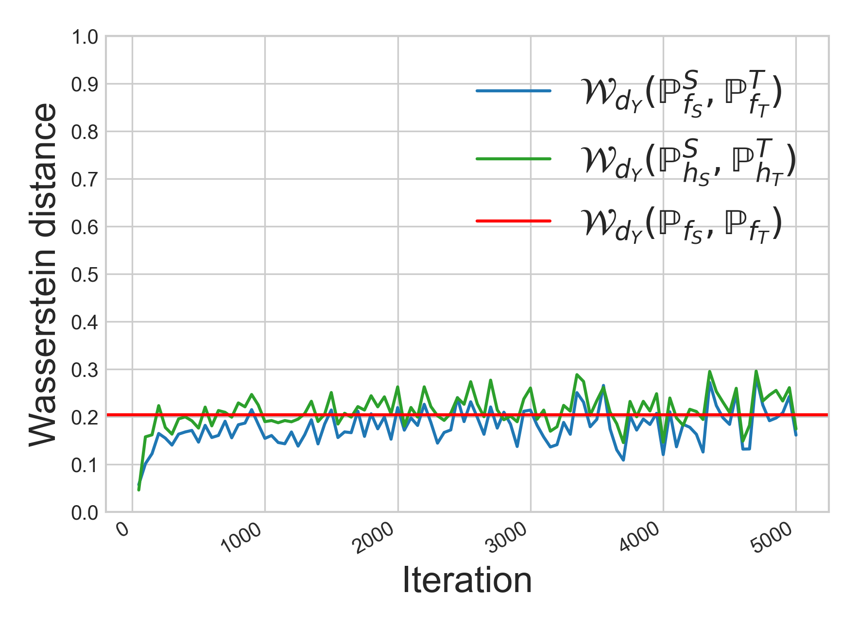
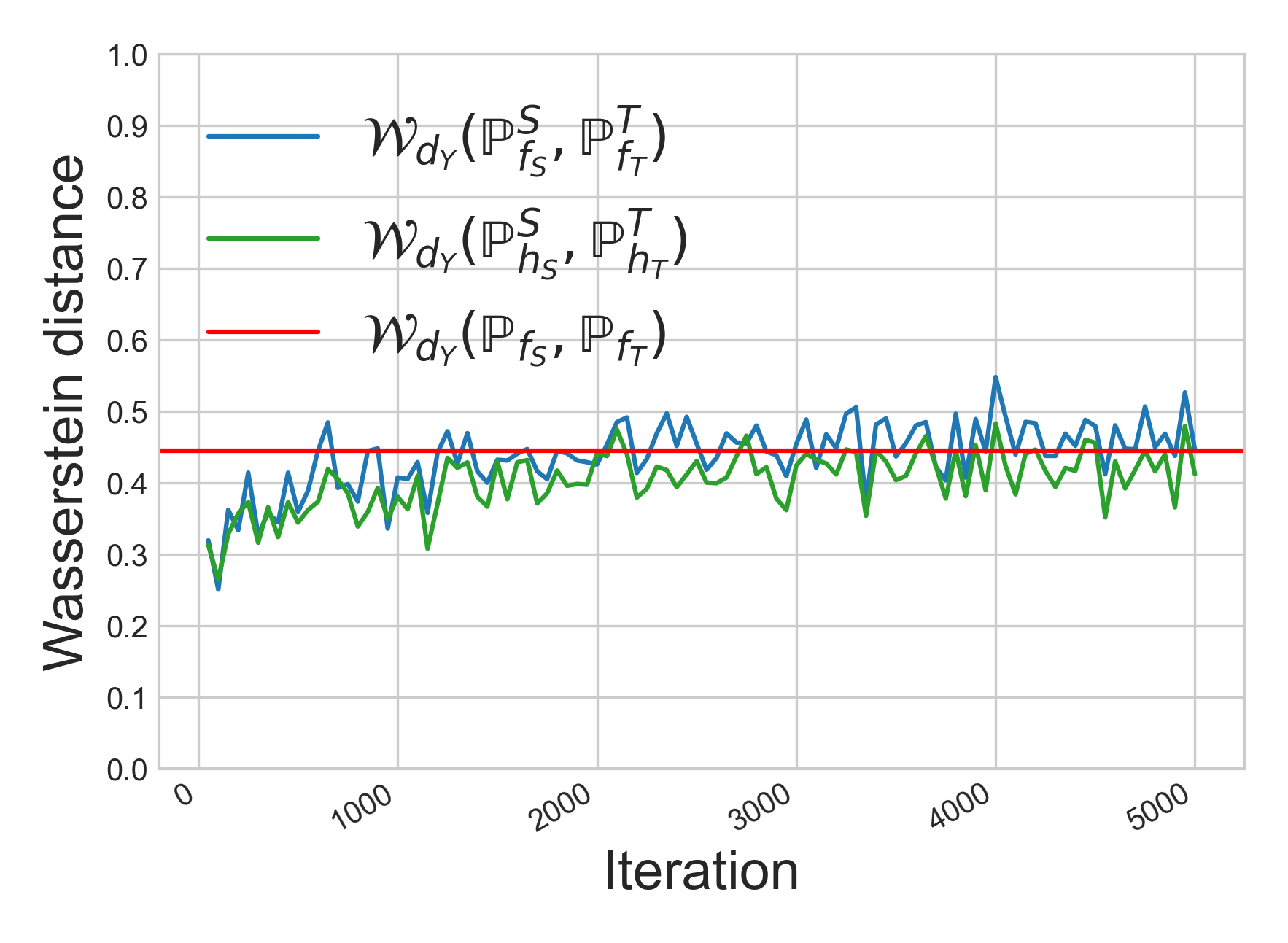
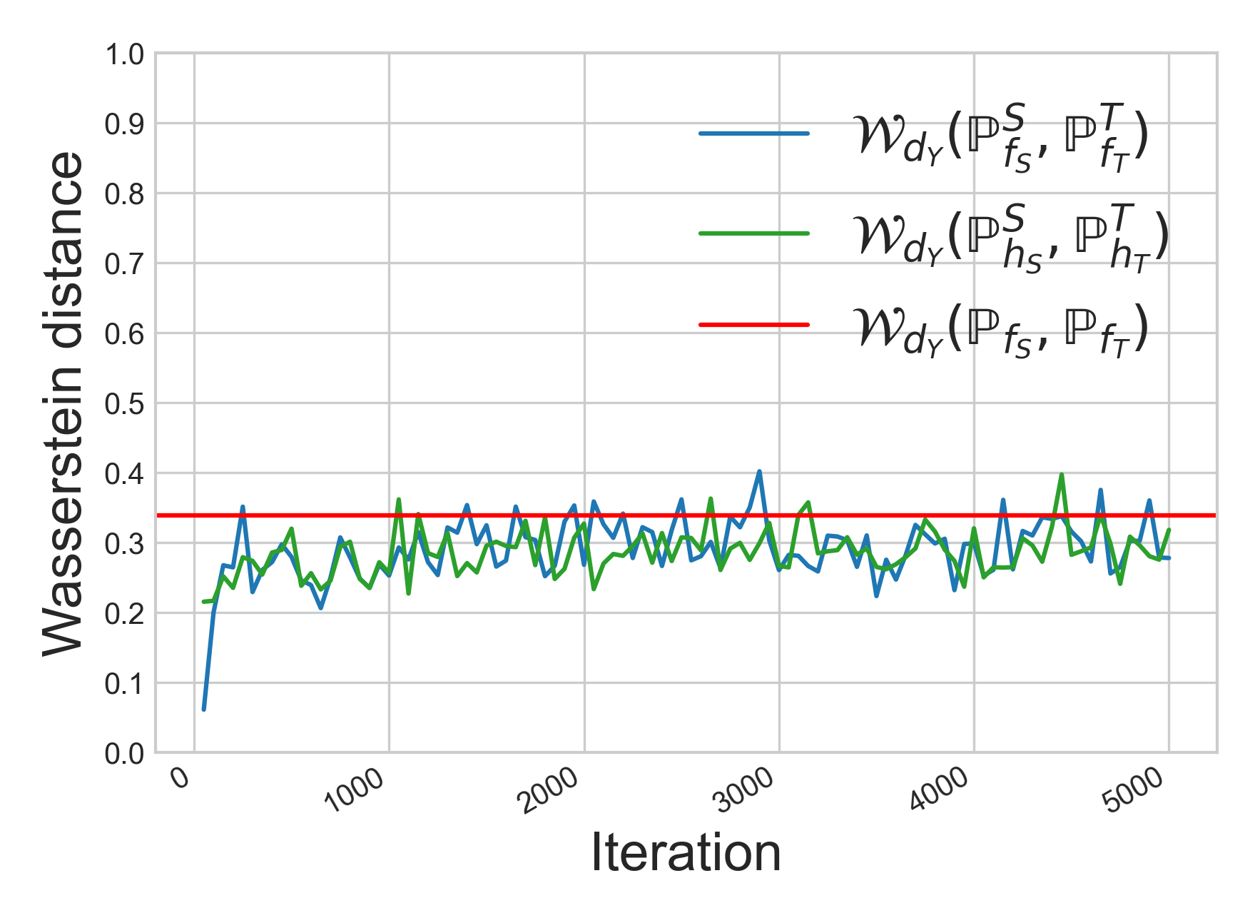
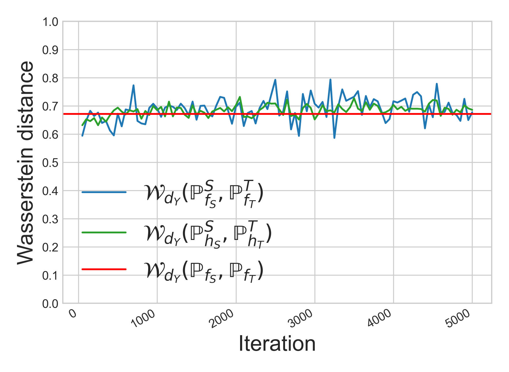
Label shift estimation: In this experiment, we show how to evaluate the label shift if we know the labeling mechanisms of the source and target domains. We consider SVHN as the source domain and MNIST as the target domain. These two datasets have ten categorical labels which stand for the digits in . Additionally, for each source or target example , the ground-truth label of is a categorical label in . Since these labels have good separation, from part (iii) of Proposition 3, we can choose and as one-hot vectors on the simplex . Therefore, and are two discrete distributions over one-hot vectors representing the categorical labels, wherein each categorical label corresponds to the one-hot vector . The label shift between SVHN and MNIST is estimated by either or , where is chosen as distance. More specifically, is evaluated accurately via linear programming111https://pythonot.github.io/all.html, while estimating using the entropic regularized dual form with [18]. Moreover, to visualize the precision when using a probabilistic labeling mechanism to estimate the label shift, we train two probabilistic labeling functions and by minimizing the cross-entropy loss with respect to and respectively and subsequently estimate using the entropic regularized dual form with . Note that the prediction probabilities of and are now the points on the simplex .
We compute the label shift for four DA settings including the closed-set, partial-set, open-set, and universal settings. As shown in Figure 2, for all DA settings, the blue lines estimating and the green lines estimating along with batches tend to approach the red lines evaluating accurately, which illustrates the result of part (iii) in Proposition 3. We also observe that the label shifts of partial-set, open-set, and universal settings are higher than the closed-set setting as discussed in Theorem 5.
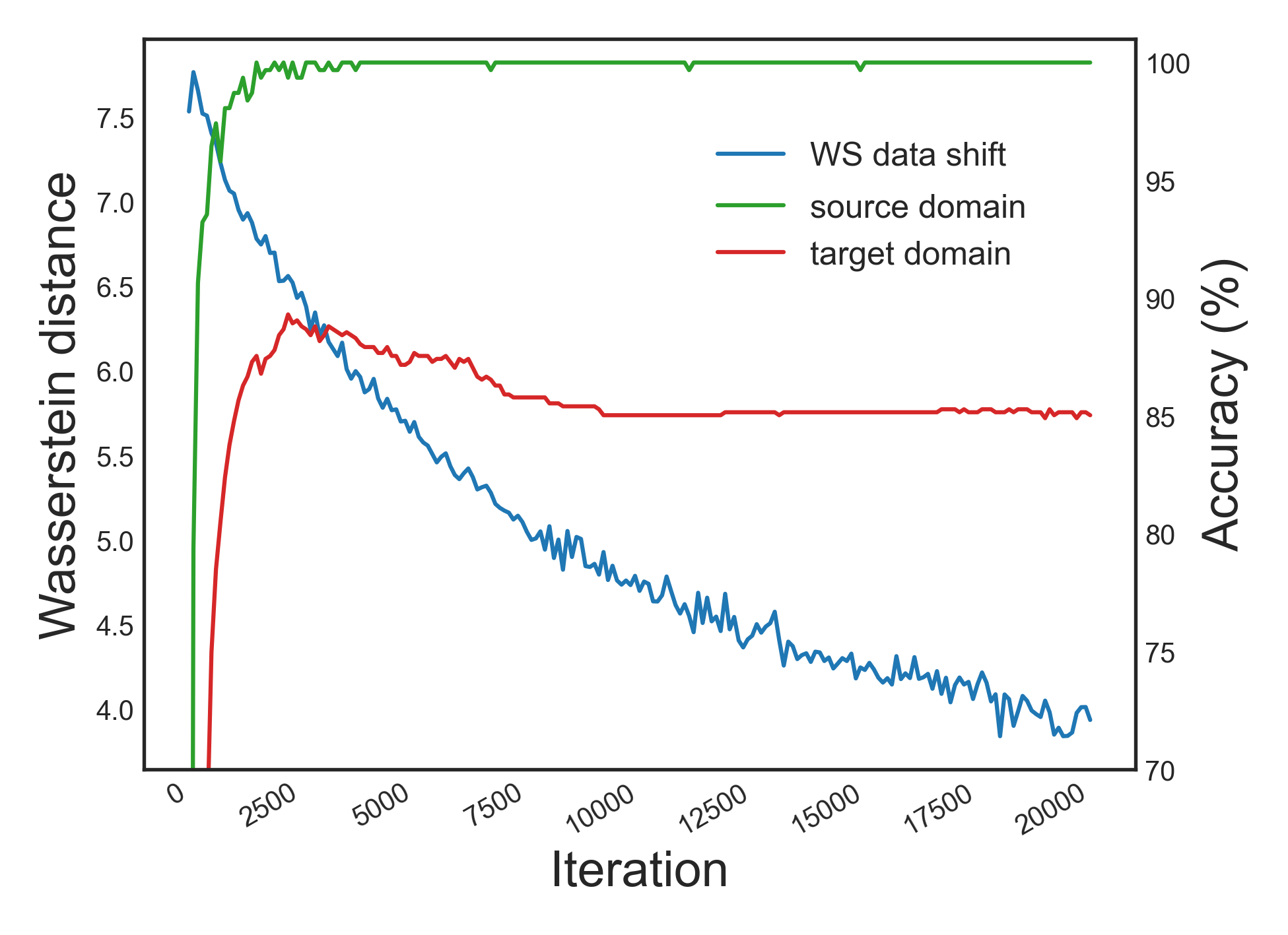
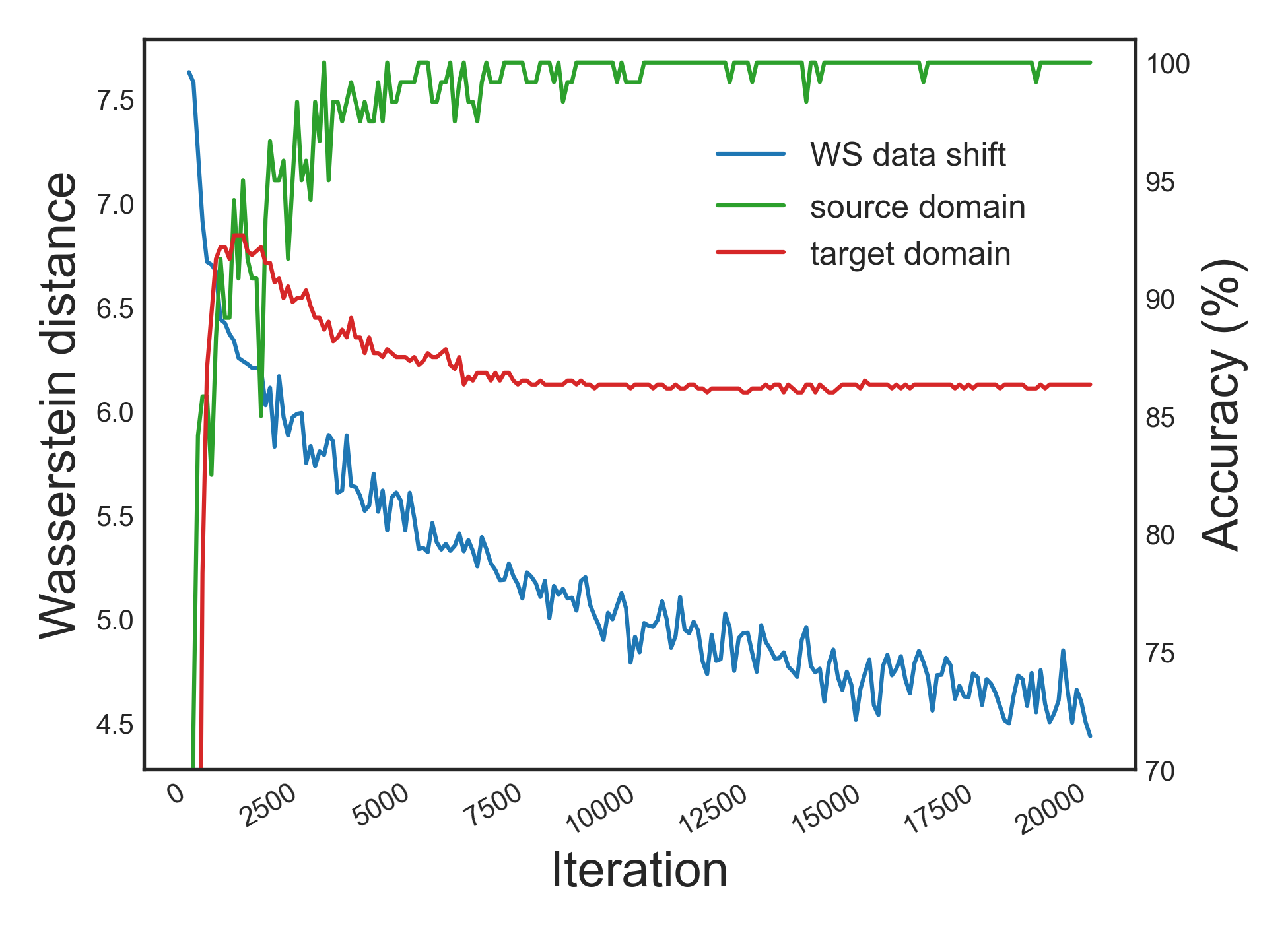
Implication on target performance: In this experiment, we demonstrate that the theoretical finding of Theorem 4 indicating that forcing learning domain-invariant representations hurts the target performance. We train a classifier , where is a feature extractor and is a classifier on top of latent representations by solving where is used to estimate for learning domain-invariant representations on the latent space. We conduct the experiments on the pairs AW (Office-31) and PI (ImageCLEF-DA) in which we measure the WS data shift on the latent space , and the source and target accuracies. As shown in Figure 3, along with the training process, while the WS data shift on the latent space consistently decreases (i.e., the latent representations become more domain-invariant), the source accuracies get saturated, but the target accuracies get hurt gradually.
4.2 Experiments of LDROT on real-world datasets
We conduct the experiments on the real-world datasets: Digits, Office-31, Office-Home, and ImageCLEF-DA to compare our LDROT to the state-of-the-art baselines, especially OT-based ones DeepJDOT [10], SWD [26], DASPOT [47], ETD [27], and RWOT [49]. Due to the space limit, we show the results for Office-31 and Office-Home in Tables 1 and 2, while other results, parameter settings, and network architectures can be found in Appendix D. The experimental results indicate that our proposed method outperforms the baselines.
| Method | ArCl | ArPr | ArRw | ClAr | ClPr | ClRw | PrAr | PrCl | PrRw | RwAr | RwCl | RwPr | Avg |
|---|---|---|---|---|---|---|---|---|---|---|---|---|---|
| ResNet-50 [22] | 34.9 | 50.0 | 58.0 | 37.4 | 41.9 | 46.2 | 38.5 | 31.2 | 60.4 | 53.9 | 41.2 | 59.9 | 46.1 |
| DANN [15] | 43.6 | 57.0 | 67.9 | 45.8 | 56.5 | 60.4 | 44.0 | 43.6 | 67.7 | 63.1 | 51.5 | 74.3 | 56.3 |
| CDAN [33] | 50.7 | 70.6 | 76.0 | 57.6 | 70.0 | 70.0 | 57.4 | 50.9 | 77.3 | 70.9 | 56.7 | 81.6 | 65.8 |
| TPN [36] | 51.2 | 71.2 | 76.0 | 65.1 | 72.9 | 72.8 | 55.4 | 48.9 | 76.5 | 70.9 | 53.4 | 80.4 | 66.2 |
| SAFN [48] | 52.0 | 71.7 | 76.3 | 64.2 | 69.9 | 71.9 | 63.7 | 51.4 | 77.1 | 70.9 | 57.1 | 81.5 | 67.3 |
| DeepJDOT [10] | 48.2 | 69.2 | 74.5 | 58.5 | 69.1 | 71.1 | 56.3 | 46.0 | 76.5 | 68.0 | 52.7 | 80.9 | 64.3 |
| ETD [27] | 51.3 | 71.9 | 85.7 | 57.6 | 69.2 | 73.7 | 57.8 | 51.2 | 79.3 | 70.2 | 57.5 | 82.1 | 67.3 |
| RWOT [49] | 55.2 | 72.5 | 78.0 | 63.5 | 72.5 | 75.1 | 60.2 | 48.5 | 78.9 | 69.8 | 54.8 | 82.5 | 67.6 |
| LDROT | 57.4 | 79.6 | 82.5 | 67.2 | 79.8 | 80.7 | 66.5 | 53.3 | 82.5 | 70.9 | 57.4 | 84.8 | 71.9 |
4.3 Ablation Study for LDROT
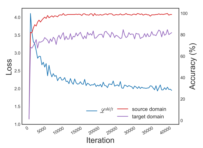
This ablation study investigates the significant meanings of the shifting term . We observe the values of together with training accuracy of the source (CI) and target (Rw) domains in Figure 4. During training, smoothly decreases, while the source and target training accuracies increases. This implies that gradually improves on the source domain, while the label shift between and gradually reduces, guiding to improve on the target domain. This observation demonstrates the rational of our label shift quantity . Due to the space limitation, other ablation studies are presented in Appendix D.7.
5 Conclusion
In this paper, we study label shift between the source and target domains in a general DA setting. Our main workaround is to consider valid transformations transporting the target to source domains allowing us to align the source and target examples and rigorously define the label shift between two domains. We then connect the proposed label shift to optimal transport theory and develop further theory to inspect the properties of DA under various DA settings (e.g., closed-set, partial-set, open-set, or universal setting). Furthermore inspired from theory development, we propose Label and Data Shift Reduction via Optimal Transport (LDROT) which can mitigate data and label shifts simultaneously. We conduct comprehensive experiments to verify our theoretical findings and compare LDROT against state-of-the-art baselines to demonstrate its merits.
References
- [1] M. Abadi, A. Agarwal, P. Barham, E. Brevdo, Z. Chen, C. Citro, G. S. Corrado, A. Davis, J. Dean, M. Devin, et al. Tensorflow: Large-scale machine learning on heterogeneous distributed systems. arXiv preprint arXiv:1603.04467, 2016.
- [2] M. Arjovsky, S. Chintala, and L. Bottou. Wasserstein generative adversarial networks. In D. Precup and Y. W. Teh, editors, Proceedings of the 34th International Conference on Machine Learning, volume 70 of Proceedings of Machine Learning Research, pages 214–223. PMLR, 06–11 Aug 2017.
- [3] S. Ben-David, J. Blitzer, K. Crammer, A. Kulesza, F. Pereira, and J. W. Vaughan. A theory of learning from different domains. Mach. Learn., 79(1-2):151–175, May 2010.
- [4] S. Ben-David and R. Urner. On the hardness of domain adaptation and the utility of unlabeled target samples. In Proceedings of the 23rd International Conference on Algorithmic Learning Theory, pages 139–153, 2012.
- [5] S. Ben-David and R. Urner. Domain adaptation—can quantity compensate for quality? Annals of Mathematics and Artificial Intelligence, 70(3):185–202, Mar. 2014.
- [6] Z. Cao, K. You, M. Long, J. Wang, and Q. Yang. Learning to transfer examples for partial domain adaptation. CoRR, abs/1903.12230, 2019.
- [7] O. Chapelle and A. Zien. Semi-supervised classification by low density separation. In AISTATS, volume 2005, pages 57–64. Citeseer, 2005.
- [8] C. Cortes, M. Mohri, and A. M. Medina. Adaptation based on generalized discrepancy. The Journal of Machine Learning Research, 20(1):1–30, 2019.
- [9] N. Courty, R. Flamary, A. Habrard, and A. Rakotomamonjy. Joint distribution optimal transportation for domain adaptation. In Advances in Neural Information Processing Systems, pages 3730–3739, 2017.
- [10] B. B. Damodaran, B. Kellenberger, R. Flamary, D. Tuia, and N. Courty. Deepjdot: Deep joint distribution optimal transport for unsupervised domain adaptation. In V. Ferrari, M. Hebert, C. Sminchisescu, and Y. Weiss, editors, Computer Vision - ECCV 2018 - 15th European Conference, Munich, Germany, September 8-14, 2018, Proceedings, Part IV, volume 11208 of Lecture Notes in Computer Science, pages 467–483, 2018.
- [11] Z. Deng, Y. Luo, and J. Zhu. Cluster alignment with a teacher for unsupervised domain adaptation, 2019.
- [12] D. M. Endres and J. E. Schindelin. A new metric for probability distributions. IEEE Trans. Inf. Theor., 49(7):1858–1860, 2006.
- [13] G. French, M. Mackiewicz, and M. Fisher. Self-ensembling for visual domain adaptation. In International Conference on Learning Representations, 2018.
- [14] Y. Ganin and V. Lempitsky. Unsupervised domain adaptation by backpropagation. In Proceedings of the 32nd International Conference on International Conference on Machine Learning - Volume 37, ICML’15, pages 1180–1189, 2015.
- [15] Y. Ganin, E. Ustinova, H. Ajakan, P. Germain, H. Larochelle, F. Laviolette, M. Marchand, and V. Lempitsky. Domain-adversarial training of neural networks. J. Mach. Learn. Res., 17(1):2096–2030, jan 2016.
- [16] S. Garg, Y. Wu, S. Balakrishnan, and Z. Lipton. A unified view of label shift estimation. In H. Larochelle, M. Ranzato, R. Hadsell, M. F. Balcan, and H. Lin, editors, Advances in Neural Information Processing Systems, volume 33, pages 3290–3300. Curran Associates, Inc., 2020.
- [17] S. Garg, Y. Wu, S. Balakrishnan, and Z. Lipton. A unified view of label shift estimation. In H. Larochelle, M. Ranzato, R. Hadsell, M. F. Balcan, and H. Lin, editors, Advances in Neural Information Processing Systems, volume 33, pages 3290–3300. Curran Associates, Inc., 2020.
- [18] A. Genevay, M. Cuturi, G. Peyré, and F. Bach. Stochastic optimization for large-scale optimal transport. In Advances in Neural Information Processing Systems, volume 29. Curran Associates, Inc., 2016.
- [19] P. Germain, A. Habrard, F. Laviolette, and E. Morvant. A PAC-Bayesian approach for domain adaptation with specialization to linear classifiers. In Proceedings of the 30th International Conference on International Conference on Machine Learning, ICML’13, 2013.
- [20] P. Germain, A. Habrard, F. Laviolette, and E. Morvant. A new PAC-Bayesian perspective on domain adaptation. In Proceedings of the 33rd International Conference on International Conference on Machine Learning - Volume 48, ICML’16, pages 859–868, 2016.
- [21] Y. Grandvalet and Y. Bengio. Semi-supervised learning by entropy minimization. In Advances in Neural Information Processing Systems, volume 17. MIT Press, 2004.
- [22] K. He, X. Zhang, S. Ren, and J. Sun. Deep residual learning for image recognition. In 2016 IEEE Conference on Computer Vision and Pattern Recognition (CVPR), pages 770–778, 2016.
- [23] F. D. Johansson, D. Sontag, and R. Ranganath. Support and invertibility in domain-invariant representations. In Proceedings of Machine Learning Research, volume 89, pages 527–536, 2019.
- [24] D. Kingma and J. Ba. Adam: A method for stochastic optimization. arXiv preprint arXiv:1412.6980, 2014.
- [25] T. Le, T. Nguyen, N. Ho, H. Bui, and D. Phung. Lamda: Label matching deep domain adaptation. In M. Meila and T. Zhang, editors, Proceedings of the 38th International Conference on Machine Learning, volume 139 of Proceedings of Machine Learning Research, pages 6043–6054. PMLR, 18–24 Jul 2021.
- [26] C. Lee, T. Batra, M. H. Baig, and D. Ulbricht. Sliced Wasserstein discrepancy for unsupervised domain adaptation. In IEEE Conference on Computer Vision and Pattern Recognition, CVPR 2019, Long Beach, CA, USA, June 16-20, 2019, pages 10285–10295. Computer Vision Foundation / IEEE, 2019.
- [27] M. Li, Y. Zhai, Y. Luo, P. Ge, and C. Ren. Enhanced transport distance for unsupervised domain adaptation. In IEEE/CVF Conference on Computer Vision and Pattern Recognition (CVPR), June 2020.
- [28] T. Lin, N. Ho, X. Chen, M. Cuturi, and M. I. Jordan. Fixed-support Wasserstein barycenters: Computational hardness and fast algorithm. In NeurIPS, pages 5368–5380, 2020.
- [29] T. Lin, N. Ho, and M. Jordan. On efficient optimal transport: An analysis of greedy and accelerated mirror descent algorithms. In ICML, pages 3982–3991, 2019.
- [30] T. Lin, N. Ho, and M. I. Jordan. On the efficiency of the Sinkhorn and Greenkhorn algorithms and their acceleration for optimal transport. ArXiv Preprint: 1906.01437, 2019.
- [31] Z. Lipton, Y.-X. Wang, and A. Smola. Detecting and correcting for label shift with black box predictors. In J. Dy and A. Krause, editors, Proceedings of the 35th International Conference on Machine Learning, volume 80 of Proceedings of Machine Learning Research, pages 3122–3130. PMLR, 10–15 Jul 2018.
- [32] M. Long, Y. Cao, J. Wang, and M. Jordan. Learning transferable features with deep adaptation networks. In F. Bach and D. Blei, editors, Proceedings of the 32nd International Conference on Machine Learning, volume 37 of Proceedings of Machine Learning Research, pages 97–105, Lille, France, 2015.
- [33] M. Long, Z. Cao, J. Wang, and M. I. Jordan. Conditional adversarial domain adaptation. In S. Bengio, H. Wallach, H. Larochelle, K. Grauman, N. Cesa-Bianchi, and R. Garnett, editors, Advances in Neural Information Processing Systems 31, pages 1640–1650. Curran Associates, Inc., 2018.
- [34] Y. Mansour, M. Mohri, and A. Rostamizadeh. Domain adaptation with multiple sources. In D. Koller, D. Schuurmans, Y. Bengio, and L. Bottou, editors, Advances in Neural Information Processing Systems 21, pages 1041–1048. 2009.
- [35] T. Miyato, S. Maeda, M. Koyama, and S. Ishii. Virtual adversarial training: A regularization method for supervised and semi-supervised learning. IEEE Transactions on Pattern Analysis and Machine Intelligence, 41(8):1979–1993, Aug 2019.
- [36] Y. Pan, T. Yao, Y. Li, Y. Wang, C. Ngo, and T. Mei. Transferrable prototypical networks for unsupervised domain adaptation. In CVPR, pages 2234–2242, 2019.
- [37] G. Peyré and M. Cuturi. Computational optimal transport: With applications to data science. Foundations and Trends® in Machine Learning, 11(5-6):355–607, 2019.
- [38] I. Redko, A. Habrard, and M. Sebban. Theoretical analysis of domain adaptation with optimal transport. In Joint European Conference on Machine Learning and Knowledge Discovery in Databases, pages 737–753, 2017.
- [39] F. Santambrogio. Optimal transport for applied mathematicians. Birkäuser, NY, pages 99–102, 2015.
- [40] R. Shu, H. Bui, H. Narui, and S. Ermon. A DIRT-t approach to unsupervised domain adaptation. In International Conference on Learning Representations, 2018.
- [41] B. Sun and K. Saenko. Deep coral: Correlation alignment for deep domain adaptation. In G. Hua and H. Jégou, editors, Computer Vision – ECCV 2016 Workshops, pages 443–450, Cham, 2016. Springer International Publishing.
- [42] R. Tachet des Combes, H. Zhao, Y.-X. Wang, and G. J. Gordon. Domain adaptation with conditional distribution matching and generalized label shift. Advances in Neural Information Processing Systems, 33, 2020.
- [43] E. Tzeng, J. Hoffman, T. Darrell, and K. Saenko. Simultaneous deep transfer across domains and tasks. CoRR, 2015.
- [44] E. Tzeng, J. Hoffman, K. Saenko, and T. Darrell. Adversarial discriminative domain adaptation. In 2017 IEEE Conference on Computer Vision and Pattern Recognition (CVPR), pages 2962–2971, 2017.
- [45] L. van der Maaten and G. Hinton. Visualizing data using t-SNE. Journal of Machine Learning Research, 9:2579–2605, 2008.
- [46] C. Villani. Optimal Transport: Old and New. Grundlehren der mathematischen Wissenschaften. Springer Berlin Heidelberg, 2008.
- [47] Y. Xie, M. Chen, H. Jiang, T. Zhao, and H. Zha. On scalable and efficient computation of large scale optimal transport. In K. Chaudhuri and R. Salakhutdinov, editors, Proceedings of the 36th International Conference on Machine Learning, volume 97 of Proceedings of Machine Learning Research, pages 6882–6892, Long Beach, California, USA, 09–15 Jun 2019. PMLR.
- [48] R. Xu, G. Li, J. Yang, and L. Lin. Larger norm more transferable: An adaptive feature norm approach for unsupervised domain adaptation. In 2019 IEEE/CVF International Conference on Computer Vision (ICCV), pages 1426–1435, 2019.
- [49] R. Xu, P. Liu, L. Wang, C. Chen, and J. Wang. Reliable weighted optimal transport for unsupervised domain adaptation. In CVPR 2020, June 2020.
- [50] Y. Zhang, Y. Liu, M. Long, and M. I. Jordan. Bridging theory and algorithm for domain adaptation. CoRR, abs/1904.05801, 2019.
- [51] Y. Zhang, H. Tang, K. Jia, and M. Tan. Domain-symmetric networks for adversarial domain adaptation. 2019 IEEE/CVF Conference on Computer Vision and Pattern Recognition (CVPR), pages 5026–5035, 2019.
- [52] H. Zhao, R. T. Des Combes, K. Zhang, and G. Gordon. On learning invariant representations for domain adaptation. In International Conference on Machine Learning, pages 7523–7532, 2019.
Supplement to “On Label Shift in Domain Adaptation
via Wasserstein Distance”
In this appendix, we collect several proofs and remaining materials that are deferred from the main paper.
-
•
In Appendix A, we present notations and definitions that are deferred from the main text including optimal transport and entropic regularized Wasserstein distance.
-
•
In Appendix B, we present proofs of all the key results.
-
•
In Appendix C, we present proofs of the remaining results, including the derivation of the dual form of entropic regularized optimal transport.
-
•
In Appendix D, we provide training specification and additional experimental results.
Appendix A Notations and definitions
In this appendix, we provide notations, notions, and definitions that are used in the main text.
A.1 Optimal Transport
Given two probability measures and and a cost function or ground metric , under the conditions stated in the below theorem (cf. Theorems 1.32 and 1.33 [39]), the primal form of Wasserstein (WS) distance [39] is defined as:
| (12) | ||||
| (13) |
where specifies the set of joint distributions over which admits and as marginals. The first definition is known as Monge problem (MP), while the second one is known as Kantorovich problem (KP). We now restate the sufficient conditions for which (MP) and (KP) are equivalent (cf. Theorems 1.32 and 1.33 [39]).
Theorem 7.
If and are compact, Polish metric spaces, and are atomless, and is a lower semi-continuous function, then (KP) is equivalent to (MP) in the sense that two infima are equal.
In addition, under some mild conditions as stated in Theorem 5.10 in [46], we can replace the primal form by its corresponding dual form
| (14) |
where and is the -transform of function defined as
A.2 Entropic Regularized Duality
To enable the application of optimal transport in machine learning and deep learning, Genevay et al. [18]developed an entropic regularized dual form, which had been shown to have favorable computational complexities [29, 30, 28]. First, they proposed to add an entropic regularization term to the primal form in (13)
| (15) |
where is the regularization rate, is the Kullback-Leibler (KL) divergence, and represents the specific coupling in which and are independent. Note that when , approaches and the optimal transport plan of (15) also weakly converges to the optimal transport plan of (13). In practice, we set to be a small positive number, hence is very close to . Second, using the Fenchel-Rockafellar theorem, they obtained the following dual form w.r.t. the potential
| (16) |
where .
A.3 Preliminaries
Notions.
For a positive integer and a real number , indicates the set while denotes the -norm of a vector . Let and be the label sets of the source and target domains that have and elements, respectively. Meanwhile, stands for the label set of both domains which has the cardinality of . Subsequently, we denote , , and as the simplices corresponding to , and respectively. Finally, let and be the labeling functions of the source and target domains, respectively, by filling zeros for the missing labels.
We first examine a general supervised learning setting. Consider a hypothesis in a hypothesis class and a labeling function (i.e., and where with the number of classes ). Let be a metric over . We further define the general loss of the hypothesis w.r.t. the data distribution and the labeling function as:
Next we consider a domain adaptation setting in which we have a source space endowed with a distribution and the density function and a target space endowed with a distribution and the density function . Let and be the labeling functions of the source and target domains respectively. It appears that and are the source and target joint distributions of pairs respectively. Note that for a categorical label , and represent the th element of the prediction probabilities and .
Appendix B Proofs of all the key results
In this appendix, we provide useful lemmas and proofs for main results in the paper.
B.1 Useful Lemmas
Lemma 8.
If , there exists .
Proof.
Let denote as the joint distribution of the samples where and as the joint distribution of the samples where . It is obvious that is a joint distribution of and and is a joint distribution of and . According to the gluing lemma (see Lemma 5.5 in [39]), there exists a joint distribution such that for any draw then , , and .
Let be the distribution of samples (i.e., the projection of onto the first and fourth dimensions). This follows that is a joint distribution of and (i.e., ). In addition, since , , since , , and . Therefore, we reach .
We note that in the above proof, we employ a general form of the gluing lemma for 4 distributions and spaces. The proof is mainly based on the gluing lemma for 3 distributions and spaces and trivial. ∎
Lemma 9.
Let be defined with respect to the family as follows:
where and lie on the latent space . For any and , if leads to , then is a proper metric.
Proof.
First, and means , which leads to . Second, it is obvious that .
Given any , we have
Therefore, is a proper metric. ∎
B.2 Proof and Corollary of Proposition 2
Proof.
(i) First, we will prove that . Let be such that where supp indicates the support of a distribution. We can express as
with and . Define . We claim that . Observe first that for any , we have where . Next, let be any measurable set and denote . Then by using the observation above and the fact , we obtain
or equivalently, . It follows from the fact that , which gives
In order to prove the reverse inequality, let us consider any maps satisfying . Define a map as , we will show that . Indeed, let be any measurable sets and take . Then, as
we have
which means . As a result,
By combining the above two inequalities, we obtain the desired equality
(ii) First, let . According to Lemma 8, there exists such that . Then, we find that
Therefore, we arrive at
Second, let , we denote . We then have
This follows that
Hence, the proof is completely done. ∎
Corollary 10.
The following inequality holds
Proof.
According to Proposition 1, we have:
Then by choosing L as the identity map (i.e., for all ), we obtain:
∎
B.3 Proof of Theorem 4
First, we will show that
By using the triangle inequality for the Wasserstein distance with respect to the metric , we have
Here we note that for , we use the triangle inequality and for , we invoke Corollary 10.
It is sufficient to prove that
Indeed, let and denote . Then, we have , and
Therefore, we obtain
Finally, we reach
Hence, we have proved our claim.
B.4 Proof of Theorem 6
Using triangle inequality, we have
We further derive
We denote . It appears that and . Therefore, we have
Finally, we reach
As a consequence, we obtain the conclusion of the theorem.
Appendix C Proof of the remaining results
C.1 Proof of Proposition 3
Denote by and the marginal distributions of the source and target domain labels, i.e., and . Let be the discrete measure on the vertices of putting mass on the one-hot representation of , . For when , the following holds:
(i) , where the constant can be viewed as a reconstruction term: ;
(ii) ;
(iii) In the setting that and are mixtures of well-separated Gaussian distributions, i.e.,
with , in which denotes the operator norm and is sufficiently large, we have
| (17) |
where is a small constant depending on , and it goes to 0 as .
(iv) In the anti-causal setting, where for all ,
| (18) |
Proof.
(i) Let and be two arbitrary maps such that and . We have the following triangle inequality:
Therefore, we obtain
Note that, the derivation in is due to , hence gaining
As a consequence, we find that
(ii) We will show that for all transformation satisfying ,
| (19) |
and then take the infimum of the LHS, which directly leads to the conclusion. Indeed, by applying Jensen inequality, we find that
We have thus proved our claim.
(iii) Consider ’s as one-hot vectors, i.e., vertices of the simplex. By the fact that Wasserstein distances on simplex are no greater than , we have
Besides, by triangle inequalities,
| (20) |
Thus, we only need to prove the claimed bounds for and . Because the proofs are similar for the source and target, in the followings, we drop the superscript for the ease of notations. We first show that the mass of concentrates near the vertices, i.e., there exists being small numbers depends on such that, for ,
| (21) |
Indeed, for all , let . Denote the dimension of to be and the Chi-square distribution with degree of freedom. We have the following tail bound:
Hence, we obtain that
where . Besides, if then for any , by triangle inequalities and the definition of the operator norm,
where the above inequalites are due to our assumption and the fact that
Hence, for all and , we have
Combining the above inequality with Bayes’ rule leads to
where . This means the difference between labeling function at and is bounded as follows
Choosing , by the fact that implies , we have
Putting the above results together, we find that
Due to the continuity of , we can also shrink such that the inequality still holds and the left-hand side is positive and we get our claim (21).
Now let and be a set containing for all satisfying and is a partition of . Let be the density of . It can be seen that
is the density function of a coupling between and . Hence, we have the following inequalities:
which goes to 0 exponentially fast when grows to infinity. Plugging the above inequality into equation (20), we obtain the conclusion of part (iii) of the proposition.
(iv) Let be conditional measure of given . By using the law of total probability, we have
| (22) |
Given the above equations, some simple algebraic transformations would lead to
| (23) |
Now let and choose such that is a valid coupling of and . By the convexity of Wasserstein distance, we have
| (24) |
As the distance between two arbitrary points on the simplex is not greater than , neither is the Wasserstein distance between any two measures on . Therefore,
| (25) |
Besides, we find that
Similarly, since for all , we could also obtain
Consequently,
| (26) |
Combining equations (25) and (26), we have the conclusion of part (iv). ∎
C.2 Proof of Theorem 5
Before providing the proof of Theorem 5, we first introduce a lemma which facilitates our later arguments.
Lemma 11.
Let and be two probability measures on . Denote by () and () the marginal distributions of () on the first dimensions and the last dimensions, respectively, where . We have
| (27) |
Proof.
Let be the optimal coupling of and , and is a random vector having law , we have . Denote by and the marginal distribution of and , respectively. It can be seen that is a coupling of and while is a coupling of and . Hence,
where is a vector including the first coordinates of , whereas contains the last elements of , and similar definitions apply for and . ∎
Now, we come back to the proof of Theorem 2.
Proof of Theorem 5:
(i)
We consider two random vectors and . Recall that and are the marginal distributions of and on their first dimensions, respectively, while denotes the marginal of on the space of variables having labels in the set . Since , we have
-
1.
, ;
-
2.
, ,
where denotes the zero vector in for .
Let be the distribution of ,
the distribution of
.
As the simplex is an dimensional manifold in
, the Wasserstein distance between
and can be written as
where
and
.
As , it can be deduced that
Besides, according to Lemma 11, we get
Putting the above two inequalities together, we obtain the conclusion that
| (28) |
(ii)
Part (ii) is done similarly to part (i). Therefore, it is omitted.
(iii)
Let and . Assume that and . It follows from the definitions of and that
-
1.
, ;
-
2.
, ;
-
3.
, .
Let be the distribution of ,
and be the distribution of
.
By using the same arguments as in part (i), we get .
Next, applying Lemma 11 twice, we obtain
As a consequence, we have proved our claim in part (iii).
C.3 Proofs of claims in paragraph "Remark on shifting term"
Lemma 12.
The following holds:
Proof.
(i) Applying the same arguments as in Proposition 1, we have
| (29) |
where such that . So now we only need to prove that
| (30) |
Due to the equivalence of Monge and Kantorovich problem, we can write the RHS as
| (31) |
To prove Eq. (30), we will show that RHS is not less than LHS and inversely. Indeed, for any coupling , we have as a coupling of , therefore
Taking the infimum with respect to ,
| (32) |
Conversely, thanks to Lemma 8, for each coupling of , there exists a coupling of such that , which deduces that
Taking the infimum with respect to ,
| (33) |
Inequalities (32) and (33) together imply equation (30) and finish the proof.
∎
Appendix D Additional experiment results
D.1 More analysis about rationale of the terms used in the objective function of LDROT
Comparing to DeepJDOT [10]. The with was investigated in DeepJDOT [10]. However, ours is different from that work in some aspects: (i) similarity based dynamic weighting, (ii) clustering loss for enforcing clustering assumption for target classifier, and (iii) entropic dual form for training rather than Sinkhorn as in [10].
This objective function consists of three losses: (i) standard loss , (ii) shifting loss , and (iii) clustering loss . The standard loss is trained on the labeled source domain. The shifting loss aims to reduce both data and label shift simultaneously on the latent space by minimizing where for which is data distance on the latent space and is distance on the label simplex. Based on the theory developed, we demonstrate that minimizing this term helps to reduce both data shift (i.e., and label shift (i.e., ). Finally, the assists us in enforcing the clustering assumption to boost the generalization of the target classifier . By enforcing the clustering assumption, classifiers are encouraged to preserve the cluster structure and give the same predictions for data representations in the same cluster. It appears that when pushing target latent toward source representations via minimizing , source and target representations tend to group in clusters, hence we can strengthen and boost generalization of target classifier by enforcing it to preserve the predictions in the same clusters.
In addition, we propose a dynamic weighting for using similarities of pairs between source and target examples. For our similarity-based weighting distance, we base on pre-trained similarities to decide if we push more or fewer pairs of source and target latent representations together to reduce data and label shifts more efficiently. Definitely, if we can push groups of source and target representations with the same labels together more efficiently, we can certainly reduce both data and label shifts simultaneously.
D.2 Data preparation and pre-processing
Digits. We resize the resolution of each sample in the dataset to , and normalize the value of each pixel to the range of .
Office-31, Office-Home, and ImageCLEF-DA. We use 2048-dimensional features extracted from ResNet-50 [22] pretrained on ImageNet.
D.3 Algorithm of LDROT
We present peusocode of LDROT in Algorithm 1.
D.4 Network architecture
There are 2 types of the architecture described in Table 3, which are small (S) and large (L) networks. We use L network for Digits and S network for the other datasets. Additionally, excluding dense layers in the network, we add the batch normalization layers on top of convolutional and dense layers to reduce the overfitting problem. Finally, we implement our LDROT in Python using TensorFlow (version 1.9.0) [1], an open-source software library for Machine Intelligence developed by the Google Brain Team. All experiments are run on a computer with an NVIDIA Tesla V100 SXM2 with 16 GB memory.
| Architecture | S | L |
|---|---|---|
| Input size | ||
| Generator | instance normalization | |
| dense, ReLU | conv. 64 lReLU | |
| dropout, | conv. 64 lReLU | |
| Gaussian noise, = 1 | conv. 64 lReLU | |
| max-pool, stride 2 | ||
| dropout, | ||
| Gaussian noise, = 1 | ||
| conv. 64 lReLU | ||
| conv. 64 lReLU | ||
| conv. 64 lReLU | ||
| max-pool, stride 2 | ||
| dropout, | ||
| Gaussian noise, = 1 | ||
| conv. 8 lReLU | ||
| max-pool, stride 2 | ||
| Classifier | #classes dense, softmax | conv. 8 lReLU |
| conv. 8 lReLU | ||
| conv. 8 lReLU | ||
| global average pool | ||
| #classes dense, softmax | ||
| 1 dense, linear | 100 dense, ReLU | |
| 1 dense, linear |
D.5 Implementation details
We first present our procedure to compute the weights , which derives from the feature extraction process. For Digits, we design a network to train from scratch on labeled source examples. Then source and target features are extracted via this pretrained model. For the other datasets, we use extracted ResNet-50 features [22] and design a small network to train LDROT. During training, the features are used for first computing pairwise similarity scores and the weights after that.
For LDROT, we find that some hyper-parameters contributes substantially to the model performance, namely and . The temperature parameter , which contributes to sharpening and contrasting the weights , is fixed to . Tweaking the regularization rate is vital for scaling and we select . For trade-off parameters , we choose and for all settings. We apply Adam optimizer [24] () with Polyak averaging. The learning rate is set to and for Digits and the other datasets respectively. Additionally, in nature, our model solves the minimax optimization problem (see Eq. (13) in the main paper) in which and are updated sequentially in each iteration with five times for and one time for . Finally, we use the cosine distance for and Kullback-Leibler (KL) divergence for .
D.6 Additional results for Digits and ImageCLEF-DA
| Method | SM | MU | UM | Avg |
|---|---|---|---|---|
| DANN [14] | 85.5 | 84.9 | 86.3 | 85.6 |
| ADDA [44] | 89.2 | 85.4 | 96.5 | 90.4 |
| DeepCORAL [41] | 88.3 | 84.1 | 93.6 | 88.7 |
| CDAN [33] | 89.2 | 95.6 | 98.0 | 94.3 |
| TPN [36] | 93.0 | 92.1 | 94.1 | 93.1 |
| rRevGrad+CAT [11] | 98.8 | 94.0 | 96.0 | 96.3 |
| SWD [26] | 98.9 | 98.1 | 97.1 | 98.0 |
| DeepJDOT [10] | 96.7 | 95.7 | 96.4 | 96.3 |
| DASPOT [47] | 96.2 | 97.5 | 96.5 | 96.7 |
| ETD [27] | 97.9 | 96.4 | 96.3 | 96.9 |
| RWOT [49] | 98.8 | 98.5 | 97.5 | 98.3 |
| LDROT | 99.0 | 98.2 | 99.1 | 98.8 |
| Method | IP | PI | IC | CI | CP | PC | Avg |
|---|---|---|---|---|---|---|---|
| ResNet-50 [22] | 74.8 | 83.9 | 91.5 | 78.0 | 65.5 | 91.2 | 80.7 |
| DeepCORAL [41] | 75.1 | 85.5 | 92.0 | 85.5 | 69.0 | 91.7 | 83.1 |
| DANN [15] | 75.0 | 86.0 | 96.2 | 87.0 | 74.3 | 91.5 | 85.0 |
| ADDA [44] | 75.5 | 88.2 | 96.5 | 89.1 | 75.1 | 92.0 | 86.0 |
| CDAN [33] | 77.7 | 90.7 | 97.7 | 91.3 | 74.2 | 94.3 | 87.7 |
| TPN [36] | 78.2 | 92.1 | 96.1 | 90.8 | 76.2 | 95.1 | 88.1 |
| SymNets [51] | 80.2 | 93.6 | 97.0 | 93.4 | 78.7 | 96.4 | 89.9 |
| SAFN [48] | 79.3 | 93.3 | 96.3 | 91.7 | 77.6 | 95.3 | 88.9 |
| rRevGrad+CAT [11] | 77.2 | 91.0 | 95.5 | 91.3 | 75.3 | 93.6 | 87.3 |
| DeepJDOT [10] | 77.5 | 90.5 | 95.0 | 88.3 | 74.9 | 94.2 | 86.7 |
| ETD [27] | 81.0 | 91.7 | 97.9 | 93.3 | 79.5 | 95.0 | 89.7 |
| RWOT [49] | 81.3 | 92.9 | 97.9 | 92.7 | 79.1 | 96.5 | 90.0 |
| LDROT | 81.7 | 96.7 | 97.5 | 94.2 | 80.4 | 96.7 | 91.2 |
D.7 Ablation studies
Effects of the label shift term and the weights : To answer the question of how will the model performance be affected when the weights or in Eq. (11) is removed?, we evaluate our model on four different settings: LDROT without both the weights and the label shift (LDROT), without the weights (LDROT), without minimizing the label shift (LDROT) and a complete model (LDROT). The results on Office-Home in Table 6 dedicate the significance of and , where these components remarkably contribute to reducing the data and label shifts with 4.1% improvements on average.
| Method | ArCl | ClAr | ClRw | PrAr | RwAr | Avg |
|---|---|---|---|---|---|---|
| LDROT | 51.7 | 62.6 | 78.5 | 63.3 | 66.1 | 64.4 |
| LDROT | 56.7 | 62.3 | 79.3 | 64.0 | 66.8 | 65.8 |
| LDROT | 55.4 | 65.5 | 80.1 | 65.0 | 68.4 | 66.9 |
| LDROT | 57.4 | 67.2 | 80.7 | 66.5 | 70.9 | 68.5 |
Rationale of weigh strategy.
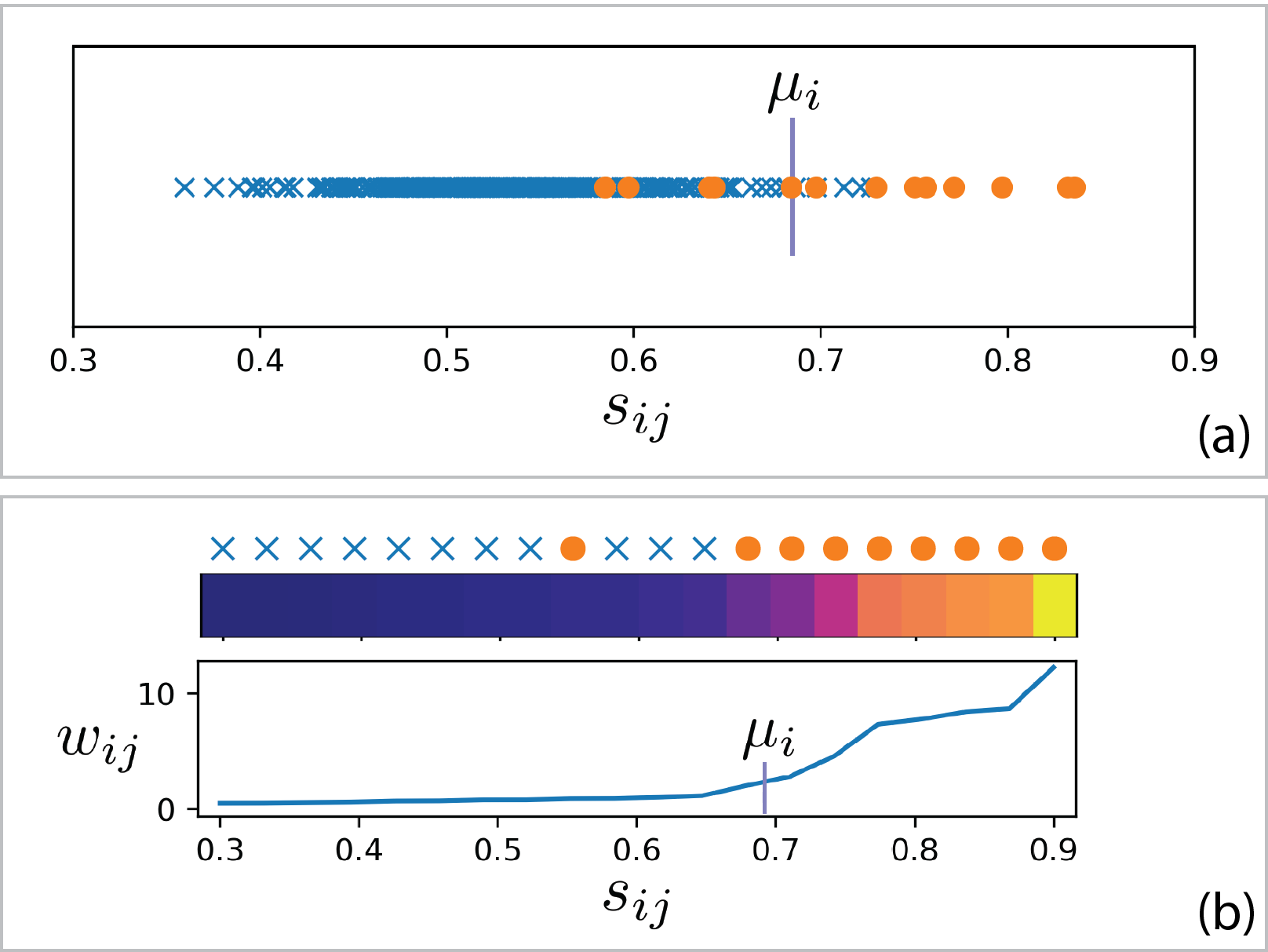
In Figure 6, we visualize the similarity scores of a randomly selected target example in a batch w.r.t. source examples using the source and target domains Amazon and Dslr of Office-31 dataset, respectively. The orange points represent the similarity scores for the same class, while the blue points represent those for different classes. It is evident that the orange values tend to bigger than the blue ones except in some outlier cases, hence if we choose as indicated, we can separate well the orange and blue values.
Feature visualization.
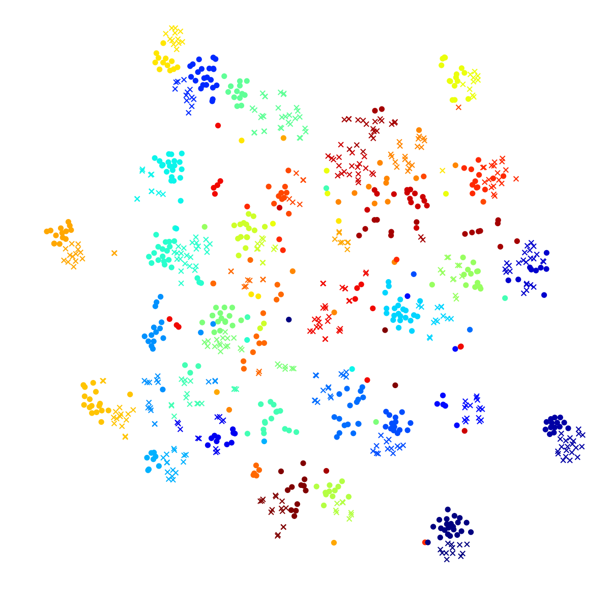
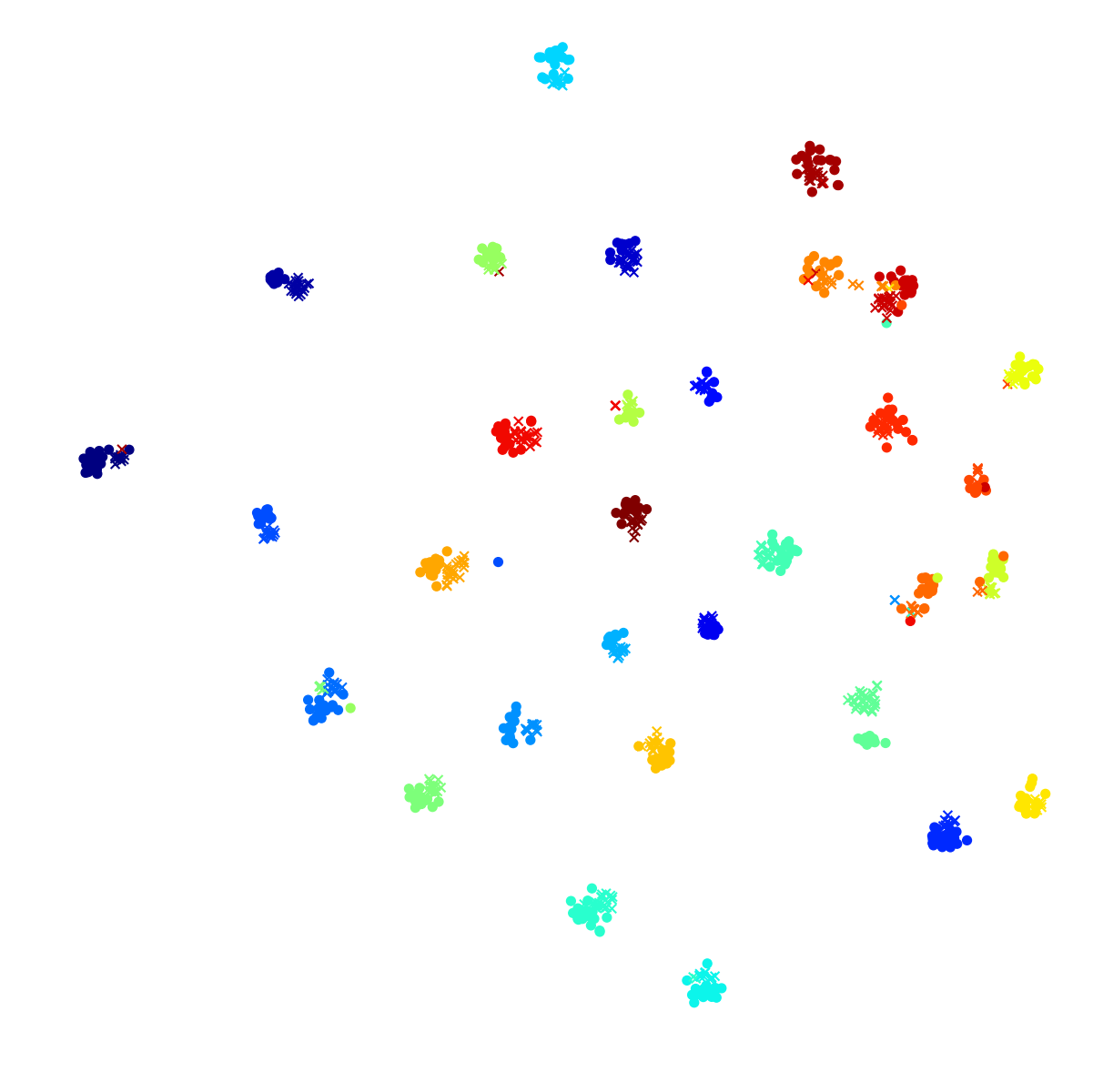
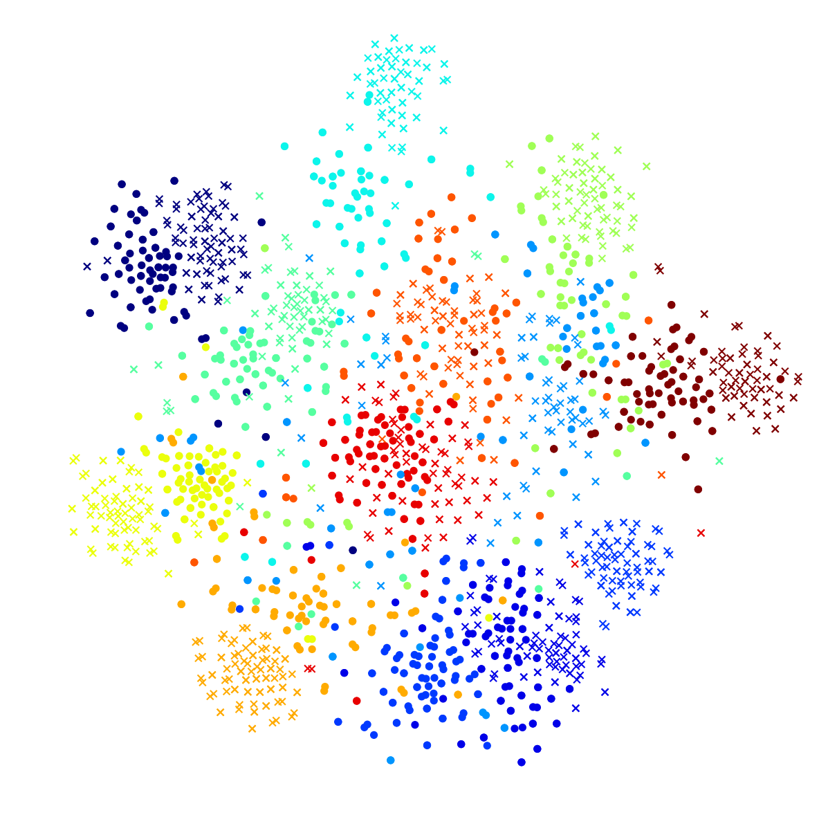
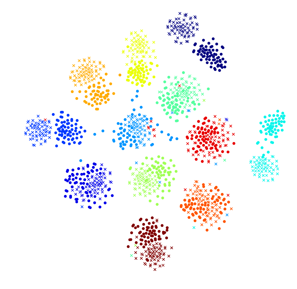
We visualize the features of ResNet-50 and our methods on A→D (Office-31) and P→C (ImageCLEF-DA) tasks by t-SNE [45] in Figure 7. The visualizations in Figure 7a and 8a show that ResNet-50 classifies quite well on source domains (A and P) but poorly on target domains (D and C). While the representation in Figure 7b and 8b is generated by our method with better alignment. LDROT achieves exactly 31 and 12 clusters corresponding to 31 and 12 classes of Office-31 and ImageCLEF-DA, which represents generalization ability of our model in which the classifier generalizes well not only on the source domain but also on the target domain.
Convergence.
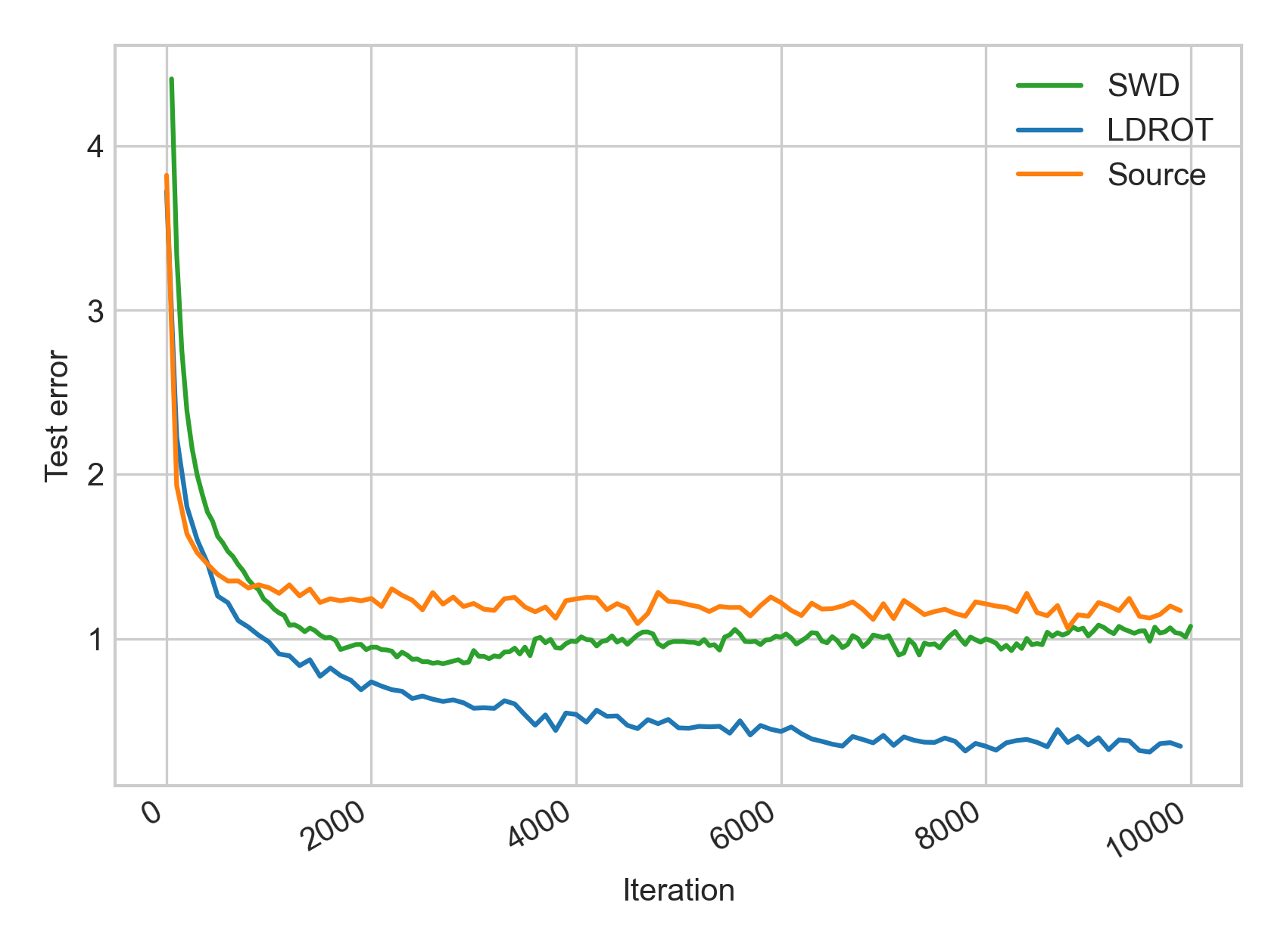
We testify the convergence of our LDROT with the test errors on A→D task, as shown in Figure 5. We conduct experiments on three methods including Source (test error is achieved with classifier trained on source data without adaptation), SWD [26], and our LDROT. For fair comparison, the methods are applied the same optimizer (Adam with learning rate of ) and batch size. The results show that the error of LDROT on the target domain is remarkably lower, which illustrates better generalization capability of the source classifier. During training, our method encourages a target sample to actively moving to a suitable group or cluster of source examples in a similarity-aware manner. This phenomenon implies that LDROT enjoys faster and stable convergence than the other settings.