Abstract

Observations in various applications are frequently represented as a time series of multidimensional arrays, called tensor time series, preserving the inherent multidimensional structure. In this paper, we present a factor model approach, in a form similar to tensor CP decomposition, to the analysis of high-dimensional dynamic tensor time series. As the loading vectors are uniquely defined but not necessarily orthogonal, it is significantly different from the existing tensor factor models based on Tucker-type tensor decomposition. The model structure allows for a set of uncorrelated one-dimensional latent dynamic factor processes, making it much more convenient to study the underlying dynamics of the time series. A new high order projection estimator is proposed for such a factor model, utilizing the special structure and the idea of the higher order orthogonal iteration procedures commonly used in Tucker-type tensor factor model and general tensor CP decomposition procedures. Theoretical investigation provides statistical error bounds for the proposed methods, which shows the significant advantage of utilizing the special model structure. Simulation study is conducted to further demonstrate the finite sample properties of the estimators. Real data application is used to illustrate the model and its interpretations.

1 Introduction

In recent years, information technology has made tensors or high-order arrays observations routinely available in applications. For example, Such data arises naturally from genomics (Alter and Golub,, 2005, Omberg et al.,, 2007), neuroimaging analysis (Zhou et al.,, 2013, Sun and Li,, 2017), recommender systems (Bi et al.,, 2018), computer vision (Liu et al.,, 2012), community detection (Anandkumar et al., 2014a, ), longitudinal data analysis (Hoff,, 2015), among others. Most of the developed tensor-based methods were designed for independent and identically distributed (i.i.d.) tensor data or tensor data with i.i.d. noise. On the other hand, in many applications, the tensors are observed over time, and hence form a tensor-valued time series. For example, the monthly import export volumes of multi-categories of products (e.g. Chemical, Food, Machinery and Electronic, and Footwear and Headwear, etc) among countries naturally form a dynamic sequence of 3-way tensor-variates, each of which representing a weighted directional transportation network. Another example is functional MRI, which typically consists hundreds of thousands of voxels observed over time. A sequence of 2-D or 3-D images can also be modeled as matrix or tensor to preserve time series. Development of statistical methods for analyzing such large scale tensor valued time series is still in its infancy.

In many settings, although the observed tensors are of high order and high dimension, there is often hidden low-dimensional structures in the tensors that can be exploited to facilitate the data analysis. Such a low-rank condition provides convenient de-composable structures and has been widely used in tensor data analysis. Two common choices of low rank tensor structures are CANDECOMP/PARAFAC (CP) structure and multilinear/Tucker structure, and each of them has their respective benefits; see the survey in Kolda and Bader, (2009). In dynamic data, the low rank structures are often realized through factor models, one of the most effective and popular dimensional reduction tools. Over the past decades, there has been a large body of literature in this area in the statistics and economics communities on factor models for vector time series. An incomplete list of the publications includes Chamberlain and Rothschild, (1983), Bai and Ng, (2002), Stock and Watson, (2002), Bai, (2003), Fan et al., (2011, 2013), Forni et al., (2000, 2004, 2005), Fan et al., (2016), Pena and Box, (1987), Pan and Yao, (2008), Lam et al., (2011), Lam and Yao, (2012). Recently, the factor model approach has been developed for analyzing high dimensional dynamic tensor time series (Wang et al.,, 2019, Chen et al.,, 2019, Chen et al., 2020a, , Chen et al., 2020b, , Chen et al.,, 2021, Han et al., 2020a, , Han et al., 2020b, ). These existing work utilizes the Tucker low rank structure in formulating the factor models. Such tensor factor model is also closely related to separable factor analysis in Fosdick and Hoff, (2014) under the array Normal distribution of Hoff, (2011).

In this paper, we investigate a tensor factor model with a CP type low rank structure, called TFM-cp. Specifically, let ${\cal X}_{t}$ be an order $K$ tensor of dimensions $d_{1}\times d_{2}\times\ldots\times d_{k}$. We assume

$${\cal X}_{t}=\sum_{i=1}^{r}w_{i}f_{it}{\mbox{\boldmath$a$}}_{i1}\otimes{\mbox{\boldmath$a$}}_{i2}\otimes\cdots\otimes{\mbox{\boldmath$a$}}_{iK}+{\cal E}_{t},\>\>\>t=1,\ldots,T,$$ (1)

where $\otimes$ denotes tensor product, $w_{i}>0$ represents the signal strength, ${\mbox{\boldmath$a$}}_{ik}$, $i=1,\ldots,r$, are unit vectors of dimension ${d_{k}}$, with $\|{\mbox{\boldmath$a$}}_{ik}\|_{2}=1$, ${\cal E}_{t}$ is a noise tensor of the same dimension as ${\cal X}_{t}$, and {$f_{it}$, $i=1,\ldots,r$} is a set of uncorrelated univariate latent factor processes. That is, the signal part of the observed tensor at time $t$ is a linear combination of $r$ rank-one tensors. These rank-one tensor are fixed and do not change over time. Here $\{{\mbox{\boldmath$a$}}_{ik},1\leq i\leq r,1\leq k\leq K\}$ are called loading vectors and not necessarily orthogonal. The dynamic of the tensor time series are driven by the $r$ univariate latent processes $f_{it}$. By stacking the tensor ${\cal X}_{t}$ into a vector, TFM-cp can be written as a vector factor model, with $r$ factors and a $d\times r$ (where $d=d_{1}\ldots d_{K}$) loading matrix with a special structure induced by the TFM-cp. More detailed discussion of the model is given in Section 2.

A standard approach for dynamic factor model estimation is through the analysis of the covariance or autocovariance of the observed process. The autocovariance of a TFM-cp process in (1) is also a tensor with a low rank CP structure. Hence potentially the estimation of (1) can be done with a tensor CP decomposion procedure. However, tensor CP decomposition is well known to be a notoriously challenging problem as it is in general NP hard to compute and the CP rank is not lower semi-continuous (Håstad,, 1990, Kolda and Bader,, 2009, Hillar and Lim,, 2013). There is a number of work in tensor CP decomposition, which is often called tensor principal component analysis (PCA) in the literature, including alternating least squares (Comon et al.,, 2009), robust tensor power methods with orthogonal components (Anandkumar et al., 2014b, ), tensor unfolding approaches (Richard and Montanari,, 2014, Wang and Lu,, 2017), rank-one alternating least squares (Anandkumar et al., 2014c, , Sun et al.,, 2017), and simultaneous matrix diagonalization (Kuleshov et al.,, 2015). See also Zhou et al., (2013), Wang and Song, (2017), Hao et al., (2020), Wang and Li, (2020) and Auddy and Yuan, (2020) among others. Although these methods can be used directly to obtain the low-rank CP components of the autocovairance tensors, they have been designed for general tensors and do not utilize the special structure induced by TFM-cp.

In this paper, we develop a new estimation procedure, named as High-Order Projection Estimators (HOPE), for TFM-cp in (1). The procedure includes a warm-start initialization using a newly developed composite principle component analysis (cPCA), and an iterative simultaneous orthogonalization scheme to refine the estimator. The procedure is designed to take the advantage of the special structure of TFM-cp whose autocovairance tensor has a specific CP structure with components close to orthogonal and of a high-order coherence in a multiplicative form. The proposed cPCA takes advantage of this feature so the initialization is better than using random projection initialization often used in generic CP decomposition algorithms. The refinement step makes use of the multiplicative coherence again and is better than the alternating least squares, the iterative projection algorithm (Han et al., 2020a, ), and other forms of the high order orthogonal iteration (HOOI) (De Lathauwer et al.,, 2000, Liu et al.,, 2014, Zhang and Xia,, 2018). Our theoretical analysis provides details of these improvements.

In the theoretical analysis, we establish statistical upper bounds on the estimation errors of the factor loading vectors for the proposed algorithms. The cPCA yields useful and good initial estimators with less restrictive conditions and the iterative algorithm provides fast statistical error rates under weak conditions, than the generic CP decomposition algorithms. For cPCA, the number of factors $r$ can increase with the dimensions of the tensor time series and is allowed to be larger than $\max_{k}d_{k}$. We also derive the statistical guarantees of the iterative algorithm to the settings where the tensor is (sufficiently) undercomplete ($r\ll\min_{k}d_{k}$). It is worth noting that the iterative refinement algorithm has much sharper statistical error upper bounds than the cPCA initial estimators.

The TFM-cp in (1) can also be written as a tensor factor model with a Tucker form with a special structure (see (2) and Remark 1 below). Hence potentially the iterative estimations procedures designed for Tucker decomposition can also be used here (Han et al., 2020a, ), ignoring the special TFM-cp structure. Again, HOPE requires less restrictive conditions and faster error rate, by fully utilizing the structure of TFM-cp. They also share the nice properties that the increase in either the dimensions $d_{1},\ldots,d_{k}$, or the sample size can improve the estimation of the factor loading vectors or spaces.

The rest of the paper is organized as follows. After a brief introduction of the basic notations used and preliminaries of tensor analysis in Section 1.1, we introduce a tensor factor model with CP low rank structure in Section 2. The estimation procedures of the factors and the loading vectors are presented in Section 3. Section 4 investigates the theoretical properties of the proposed methods. Section 5 develops some alternative algorithms to tensor factor models, and provides some simulation studies to demonstrate the numerical performance of the estimation procedures. Section 6 illustrates the model and its interpretations in real data applications. Section 7 provides a short concluding remark. All technical details are relegated to the supplementary materials.

1.1 Notation and preliminaries

The following basic notation and preliminaries will be used throughout the paper. Define $\|x\|_{q}=(x_{1}^{q}+...+x_{p}^{q})^{1/q}$, $q\geq 1$, for any vector $x=(x_{1},...,x_{p})^{\top}$. The matrix spectral norm is denoted as

$$\|A\|_{\rm S}=\max_{\|x\|_{2}=1,\|y\|_{2}=1}\|x^{\top}Ay\|_{2}.$$

For two sequences of real numbers $\{a_{n}\}$ and $\{b_{n}\}$, write $a_{n}=O(b_{n})$ (resp. $a_{n}\asymp b_{n}$) if there exists a constant $C$ such that $|a_{n}|\leq C|b_{n}|$ (resp. $1/C\leq a_{n}/b_{n}\leq C$) holds for all sufficiently large $n$, and write $a_{n}=o(b_{n})$ if $\lim_{n\to\infty}a_{n}/b_{n}=0$. Write $a_{n}\lesssim b_{n}$ (resp. $a_{n}\gtrsim b_{n}$) if there exist a constant $C$ such that $a_{n}\leq Cb_{n}$ (resp. $a_{n}\geq Cb_{n}$).

For any two tensors ${\cal A}\in\mathbb{R}^{m_{1}\times m_{2}\times\cdots\times m_{K}},{\cal B}\in\mathbb{R}^{r_{1}\times r_{2}\times\cdots\times r_{N}}$, denote the tensor product $\otimes$ as ${\cal A}\otimes{\cal B}\in\mathbb{R}^{m_{1}\times\cdots\times m_{K}\times r_{1}\times\cdots\times r_{N}}$, such that

$$({\cal A}\otimes{\cal B})_{i_{1},...,i_{K},j_{1},...,j_{N}}=({\cal A})_{i_{1},...,i_{K}}({\cal B})_{j_{1},...,j_{N}}.$$

The $k$-mode product of ${\cal A}\in\mathbb{R}^{r_{1}\times r_{2}\times\cdots\times r_{K}}$ with a matrix $U\in\mathbb{R}^{m_{k}\times r_{k}}$ is an order $K$-tensor of size $r_{1}\times\cdots r_{k-1}\times m_{k}\times r_{k+1}\times r_{K}$ and will be denoted as ${\cal A}\times_{k}U$, such that

$$({\cal A}\times_{k}U)_{i_{1},...,i_{k-1},j,i_{k+1},...,i_{K}}=\sum_{i_{k}=1}^{r_{k}}{\cal A}_{i_{1},i_{2},...,i_{K}}U_{j,i_{k}}.$$

Given ${\cal A}\in\mathbb{R}^{m_{1}\times\cdots\times m_{K}}$ and $m=\prod_{j=1}^{K}m_{j}$, let ${\rm{vec}}({\cal A})\in\mathbb{R}^{m}$ be vectorization of the matrix/tensor ${\cal A}$, $\hbox{\rm mat}_{k}({\cal A})\in\mathbb{R}^{m_{k}\times(m/m_{k})}$ the mode-$k$ matrix unfolding of ${\cal A}$, and $\hbox{\rm mat}_{k}(\hbox{\rm vec}({\cal A}))=\hbox{\rm mat}_{k}({\cal A})$.

2 A tensor factor model with a CP low rank structure

Again, we specifically consider the following tensor factor model with CP low rank structure (TFM-cp) for observations ${\cal X}_{t}\in\mathbb{R}^{d_{1}\times\cdots\times d_{K}}$, $1\leq t\leq T$,

$${\cal X}_{t}=\sum_{i=1}^{r}w_{i}f_{it}{\mbox{\boldmath$a$}}_{i1}\otimes{\mbox{\boldmath$a$}}_{i2}\otimes\cdots\otimes{\mbox{\boldmath$a$}}_{iK}+{\cal E}_{t},$$

where $f_{it}$ is the unobserved latent factor process and ${\mbox{\boldmath$a$}}_{ik}$ are the fixed unknown factor loading vectors. We assume without loss of generality, $\mathbb{E}f_{it}^{2}=1$, $\|{\mbox{\boldmath$a$}}_{ik}\|_{2}=1$, for all $1\leq i\leq r$ and $1\leq k\leq K$. Then, all the signal strengths are contained in $w_{i}$. A key assumption of TFM-cp is that the factor process $f_{it}$ is assumed to be uncorrelated across different factor processes, e.g. $\mathbb{E}f_{it-h}f_{jt}=0$ for all $i\neq j$ and some $h\geq 1$. In addition, we assume that the noise tensor ${\cal E}_{t}$ are uncorrelated (white) across time, but with an arbitrary contemporary covariance structure, following Lam and Yao, (2012), Chen et al., (2021). In this paper, we consider the case that the order of the tensor $K$ is fixed but the dimensions $d_{1},...,d_{K}\to\infty$ and rank $r$ can be fixed or diverge.

Remark 1 (Comparison with TFM-cp with a Tucker low rank structure).

Chen et al., (2021), Chen et al., 2020a , Han et al., 2020a , Han et al., 2020b studied the following tensor factor models with a Tucker low rank structure (TFM-tucker):

$${\cal X}_{t}={\cal F}_{t}\times_{1}{\mbox{\boldmath$A$}}_{1}\times\cdots\times{\mbox{\boldmath$A$}}_{K}+{\cal E}_{t},$$ (2)

where the core tensor ${\cal F}_{t}\in\mathbb{R}^{r_{1}\times\cdots r_{K}}$ is the latent factor process in a tensor form, and ${\mbox{\boldmath$A$}}_{i}$’s are $d_{i}\times r_{i}$ loading matrices. For example, when $K=2$ (matrix time series), the TFM-cp can be written as

$${\mbox{\boldmath$X$}}_{t}={\mbox{\boldmath$A$}}_{1}{\mbox{\boldmath$F$}}_{t}{\mbox{\boldmath$A$}}_{2}^{\top}+{\mbox{\boldmath$E$}}_{t},$$

where ${\mbox{\boldmath$F$}}_{t}={\rm diag}(f_{1t},\ldots,f_{rt})$, and ${\mbox{\boldmath$A$}}_{1}=({\mbox{\boldmath$a$}}_{11},\ldots,{\mbox{\boldmath$a$}}_{r1})$ and ${\mbox{\boldmath$A$}}_{2}=({\mbox{\boldmath$a$}}_{12},\ldots,{\mbox{\boldmath$a$}}_{r2})$ are matrices formed by the column vectors of ${\mbox{\boldmath$a$}}_{ik}$’s. There are three major differences between TFM-tucker and TFM-cp. First, TFM-tucker suffers a severe identification problem, as the model does not change if ${\cal F}_{t}$ is replaced by ${\cal F}_{t}\times_{k}{\mbox{\boldmath$R$}}$ and ${\mbox{\boldmath$A$}}_{k}$ replaced by ${\mbox{\boldmath$A$}}_{k}{\mbox{\boldmath$R$}}^{-1}$ for any invertible $r_{k}\times r_{k}$ matrix $R$. For $K=2$ case, ${\mbox{\boldmath$X$}}_{t}=({\mbox{\boldmath$A$}}_{1}{\mbox{\boldmath$R$}}_{1}^{-1})({\mbox{\boldmath$R$}}_{1}{\mbox{\boldmath$F$}}_{t}{\mbox{\boldmath$R$}}_{2}^{\top})({\mbox{\boldmath$A$}}_{2}{\mbox{\boldmath$R$}}_{2}^{-1})^{\top}+{\mbox{\boldmath$E$}}_{t}$ are all equivalent. Such ambiguity makes it difficult to find an ‘optimal’ representation of the model, which often lead to ad hoc and convenient representations that are difficult to interpret (Bekker,, 1986, Neudecker,, 1990, Bai and Wang,, 2014, 2015). On the other hand, TFM-cp is uniquely defined, up to sign changes, under an ordering of signal strength $w_{1}>w_{2}>\ldots>w_{r}$. As a result, the interpretation of the model becomes much easier. Second, although TFM-cp can be rewritten as a TFM-tucker with a diagonal core latent tensor consisting of the individual $f_{it}$’s, such a representation is almost impossible to arrive due to the identification problem of TFM-tucker, especially if one adopts the popular representation that the loading matrices ${\mbox{\boldmath$A$}}_{k}$ are orthonormal. In TFM-cp, the loading vectors $\{{\mbox{\boldmath$a$}}_{ik},1\leq i\leq r\}$ are also not necessarily orthogonal vectors. For $K=2$, requiring ${\mbox{\boldmath$A$}}_{1}{\mbox{\boldmath$R$}}_{1}^{-1}$ and ${\mbox{\boldmath$A$}}_{2}{\mbox{\boldmath$R$}}_{2}^{-1}$ to be orthonormal in TFM-cp makes the corresponding factor process ${\mbox{\boldmath$R$}}_{1}{\mbox{\boldmath$F$}}_{t}{\mbox{\boldmath$R$}}_{2}^{\top}$ non-diagonal, with $r^{2}$ heavily correlated components, rather than $r$ uncorrelated components. Third, TFM-cp separates the factor processes into a set of univariate time series, which enjoys great advantages in ease of modeling the dynamic with vast repository of linear and nonlinear options, as well as testing of the component series. Lastly, TFM-cp is often much more parsimonious due to its restrictions, while enjoys great flexibility. Note that TFM-tucker is also a special case of TFM-cp, as it can be written as a sum of $r=r_{1}\ldots r_{K}$ rank-one tensors, albeit with many repeated loading vectors. In applications, TFM-cp uses a much small $r$.

Remark 2.

There are two different types of factor model assumptions in the literature. One type of factor models assumes that a common factor must have impact on ‘most’ (defined asymptotically) of the time series, but allows the idiosyncratic noise (${\cal E}_{t}$) to have weak cross-correlations and weak autocorrelations; see, e.g., Forni et al., (2000), Bai and Ng, (2002), Stock and Watson, (2002), Fan et al., (2011, 2013), Chen et al., 2020a . Principle component analysis (PCA) of the sample covariance matrix is typically used to estimate the factor loading space, with various extensions. Another type of factor models assumes that the factors accommodate all dynamics, making the idiosyncratic noise ‘white’ with no autocorrelation but allowing substantial contemporary cross-correlation among the error process; see, e.g., Pena and Box, (1987), Pan and Yao, (2008), Lam et al., (2011), Lam and Yao, (2012), Wang et al., (2019). Under such assumptions, PCA is applied to the non-zero lag autocovariance matrices. In this paper, we adopt the second approach in our model development.

3 Estimation procedures

In this section, we focus on the estimation of the factors and loading vectors of model (1). The proposed procedure includes two steps: initialization using a new composite PCA (cPCA) procedure, represented as Algorithm 1, and an iterative refinement step using a new iterative simultaneous orthogonalization (ISO) procedure, represented as Algorithm 2. We call this procedure HOPE (High-Order Projection Estimators) as it repeatedly utilize high order projections on high order moments of the tensor observations. It utilizes the special structure of the model and leads to higher statistical and computational efficiency, which will be demonstrated later.

For ${\cal X}_{t}$ following (1), the lagged cross-product operator, denoted by ${\mbox{\boldmath$\mathnormal{\Sigma}$}}_{h}$, is the $(2K)$-tensor satisfying

$${\mbox{\boldmath$\mathnormal{\Sigma}$}}_{h} = \mathbb{E}\left[\sum_{t=h+1}^{T}\frac{{\cal X}_{t-h}\otimes{\cal X}_{t}}{T-h}\right]$$ (3)

$$= \sum_{i=1}^{r}\lambda_{i,h}({\mbox{\boldmath$a$}}_{i1}\otimes{\mbox{\boldmath$a$}}_{i2}\otimes\cdots\otimes{\mbox{\boldmath$a$}}_{iK})^{\otimes 2}\in\mathbb{R}^{d_{1}\times\cdots\times d_{K}\times d_{1}\times\cdots\times d_{K}},$$

for a given $h\geq 1$, where $\lambda_{i,h}=w_{i}^{2}\mathbb{E}f_{i,t-h}f_{i,t}$. Note that the tensor ${\mbox{\boldmath$\mathnormal{\Sigma}$}}_{h}$ is expressed in a CP-decomposition form with each ${\mbox{\boldmath$a$}}_{ik}$ used twice. Let $\widehat{\mbox{\boldmath$\mathnormal{\Sigma}$}}_{h}$ be the sample version of ${\mbox{\boldmath$\mathnormal{\Sigma}$}}_{h}$,

$$\widehat{\mbox{\boldmath$\mathnormal{\Sigma}$}}_{h}=\sum_{t=h+1}^{T}\frac{{\cal X}_{t-h}\otimes{\cal X}_{t}}{T-h}.$$ (4)

When ${\cal X}_{t}$ is weakly stationary and ${\cal E}_{t}$ is white noise, a nature approach to estimate the loading vectors is via minimizing the empirical squared loss

$$({\mbox{\boldmath$a$}}_{i1},{\mbox{\boldmath$a$}}_{i2},...,{\mbox{\boldmath$a$}}_{iK},1\leq i\leq r)=\operatorname*{\arg\min}_{\begin{subarray}{c}{\mbox{\boldmath$a$}}_{i1},{\mbox{\boldmath$a$}}_{i2},...,{\mbox{\boldmath$a$}}_{iK},1\leq i\leq r,\\ \|{\mbox{\boldmath$a$}}_{i1}\|_{2}=...\|{\mbox{\boldmath$a$}}_{iK}\|_{2}=1\end{subarray}}\left\|\widehat{\mbox{\boldmath$\mathnormal{\Sigma}$}}_{h}-\sum_{i=1}^{r}\lambda_{i,h}({\mbox{\boldmath$a$}}_{i1}\otimes{\mbox{\boldmath$a$}}_{i2}\otimes\cdots\otimes{\mbox{\boldmath$a$}}_{iK})^{\otimes 2}\right\|_{\rm HS}^{2},$$ (5)

where the Hilbert Schmidt norm for a tensor ${\cal A}$ is defined as $\|{\cal A}\|_{{\rm HS}}=\|\hbox{\rm vec}({\cal A})\|_{2}.$ In other words, ${\mbox{\boldmath$a$}}_{i1}\otimes{\mbox{\boldmath$a$}}_{i2}\otimes\cdots\otimes{\mbox{\boldmath$a$}}_{iK}$ can be estimated by the leading principal component of the sample auto-covariance tensor $\widehat{\mbox{\boldmath$\mathnormal{\Sigma}$}}_{h}$. However, due to the non-convexity of (5) or its variants, a straightforward implementation of many local search algorithms, such as gradient descent and alternating minimization, may easily get trapped into local optimums and result in sub-optimal statistical performance. As shown by Auffinger et al., (2013), there could be an exponential number of local optima and great majority of these local optima are far from the best low rank approximation. However, if we start from an appropriate initialization not too far from the global optimum, then a local optimum reached may be as good an estimator as the global optimum. A critical task in estimating the factor loading vectors is thus to obtain good initialization.

We develop a warm initiation procedure, the composite PCA (cPCA) procedure. Note that, if we unfold ${\mbox{\boldmath$\mathnormal{\Sigma}$}}_{h}$ into a $d\times d$ matrix ${\mbox{\boldmath$\mathnormal{\Sigma}$}}_{h}^{*}$ where $d=d_{1}\ldots d_{K}$, then (3) implies that

$${\mbox{\boldmath$\mathnormal{\Sigma}$}}_{h}^{*}=\sum_{i=1}^{r}\lambda_{i,h}{\mbox{\boldmath$a$}}_{i}{\mbox{\boldmath$a$}}_{i}^{\top},$$ (6)

a sum of $r$ rank-one matrices, each of the form ${\mbox{\boldmath$a$}}_{i}{\mbox{\boldmath$a$}}_{i}^{\top}$, where ${\mbox{\boldmath$a$}}_{i}=\hbox{\rm vec}(\otimes_{k=1}^{K}{\mbox{\boldmath$a$}}_{ik})$. This is very close to principle component decomposition of ${\mbox{\boldmath$\mathnormal{\Sigma}$}}_{h}^{*}$, except that ${\mbox{\boldmath$a$}}_{i}$’s are not necessary orthogonal in this case. However, the following intuition provides a solid justification of using PCA to obtain an estimate of ${\mbox{\boldmath$a$}}_{i}$. We call this estimator the cPCA estimator.

The accuracy of using the principle components of ${\mbox{\boldmath$\mathnormal{\Sigma}$}}_{h}^{*}$ as the estimate of ${\mbox{\boldmath$a$}}_{i}$ heavily depends on the coherence of the components, defined as $\vartheta=\max_{1\leq i<j\leq r}|{\mbox{\boldmath$a$}}_{i}^{\top}{\mbox{\boldmath$a$}}_{j}|$, the maximum correlation among the ${\mbox{\boldmath$a$}}_{i}$’s. When the components are orthogonal ($\vartheta=0$), there is no error in using PCA. The main idea of cPCA is to take advantage of the special structure of TFM-cp, which leads to a multiplicative high-order coherence of the CP components. In the following we provide an analysis of $\vartheta$ under TFM-cp.

Let ${\mbox{\boldmath$A$}}_{k}=({\mbox{\boldmath$a$}}_{1k},\ldots,{\mbox{\boldmath$a$}}_{rk})\in\mathbb{R}^{d_{k}\times r}$ be the matrix with ${\mbox{\boldmath$a$}}_{ik}$ as its columns, and ${\mbox{\boldmath$A$}}_{k}^{\top}{\mbox{\boldmath$A$}}_{k}=(\sigma_{ij,k})_{r\times r}$. As $\sigma_{ii,k}=\|{\mbox{\boldmath$a$}}_{ik}\|_{2}^{2}=1$, the correlation among columns of ${\mbox{\boldmath$A$}}_{k}$ can be measured by

$$\vartheta_{k}=\max_{1\leq i<j\leq r}|\sigma_{ij,k}|,\ \ \delta_{k}=\|{\mbox{\boldmath$A$}}_{k}^{\top}{\mbox{\boldmath$A$}}_{k}-I_{r}\|_{\rm S},\ \ \eta_{jk}=\Big{(}\sum_{i\in[K]\setminus\{j\}}\sigma_{ij,k}^{2}\Big{)}^{1/2}.$$ (7)

Similarly we use

$$\vartheta=\max_{1\leq i<j\leq r}|{\mbox{\boldmath$a$}}_{i}^{\top}{\mbox{\boldmath$a$}}_{j}|,\quad\delta=\|{\mbox{\boldmath$A$}}^{\top}{\mbox{\boldmath$A$}}-I_{r}\|_{\rm S},$$ (8)

to measure the correlation of the matrix ${\mbox{\boldmath$A$}}=({\mbox{\boldmath$a$}}_{1},\ldots,{\mbox{\boldmath$a$}}_{r})\in\mathbb{R}^{d\times r}$ with ${\mbox{\boldmath$a$}}_{i}=\hbox{\rm vec}(\otimes_{k=1}^{K}{\mbox{\boldmath$a$}}_{ik})$ and $d=\prod_{k=1}^{K}d_{k}$. It can be seen that the coherence $\vartheta$ has the bound $\vartheta\leq\prod_{k=1}^{K}\vartheta_{k}\leq\vartheta_{\max}^{K}$, due to ${\mbox{\boldmath$a$}}_{i}^{\top}{\mbox{\boldmath$a$}}_{j}=\prod_{k=1}^{K}{\mbox{\boldmath$a$}}_{ik}^{\top}{\mbox{\boldmath$a$}}_{jk}=\prod_{k=1}^{K}\sigma_{ij,k}$. The spectrum norm $\delta$ is also bounded by the multiplicative of correlation measures in (7). More specifically, we have the following proposition.

Proposition 1.

Define $\mu_{*}=\max_{j}\min_{k_{1},k_{2}}\max_{i\neq j}\prod_{k\neq k_{1},k\neq k_{2},k\in[1:K]}\sqrt{r}|\sigma_{ij,k}|/\eta_{jk}\in~{}[1,r^{K/2-1}]$ as the (leave-two-out) mutual coherence of ${\mbox{\boldmath$A$}}_{1},\ldots,{\mbox{\boldmath$A$}}_{K}$. Then, $\delta\leq\min_{1\leq k\leq K}\delta_{k}$ and

$$\delta \leq(r-1)\vartheta,\mbox{\ \ and \ \ }\vartheta\leq\prod_{k=1}^{K}\vartheta_{k}\leq\vartheta_{\max}^{K},$$ (9)

$$\delta \leq\mu_{*}r^{1-K/2}\max_{j\leq r}\prod_{k=1}^{K}\eta_{jk}\leq\mu_{*}r^{1-K/2}\prod_{k=1}^{K}\delta_{k}.$$ (10)

When (most of) the quantities in (7) are small, the products in (9) would be very small so that the ${\mbox{\boldmath$a$}}_{i}$’s are nearly orthogonal. For example, if $({\mbox{\boldmath$a$}}_{11},{\mbox{\boldmath$a$}}_{21})$ and $({\mbox{\boldmath$a$}}_{12},{\mbox{\boldmath$a$}}_{22})$ both have i.i.d. bi-variate random rows with correlation coefficients $\rho_{1}$ and $\rho_{2}$, and independent, then the correlation coefficient of $\hbox{\rm vec}({\mbox{\boldmath$a$}}_{11}\otimes{\mbox{\boldmath$a$}}_{12})$ and $\hbox{\rm vec}({\mbox{\boldmath$a$}}_{21}\otimes{\mbox{\boldmath$a$}}_{22})$ is $\rho_{1}\rho_{2}$, though the variation of the sample correlation coefficient depends on the length of the ${\mbox{\boldmath$a$}}_{ik}$’s.

Remark 3.

An incoherence condition $\vartheta_{\max}\lesssim\text{ploylog}(d_{\min})/\sqrt{d_{\min}}$ is commonly imposed in the literature for generic CP decomposition; see e.g. Anandkumar et al., 2014c , Anandkumar et al., 2014b , Sun et al., (2017), Hao et al., (2020). Proposition 1 establishes a connection between $\delta$, $\delta_{k}$ and the $\vartheta_{k}$ in such an incoherence condition. The parameters $\delta_{k}$ and $\delta$ quantify the non-orthogonality of the factor loading vectors, and play a key role in our theoretical analysis, as the performance bound of cPCA estimators involves $\delta$. Differently from the existing literature depending on $\vartheta_{\max}$, the cPCA exploits $\delta$ or the much smaller $\vartheta$ (comparing to $\vartheta_{\max}$), thus has better properties when $K\geq 2$.

The pseudo-code of cPCA is provided in Algorithm 1. Though ${\mbox{\boldmath$\mathnormal{\Sigma}$}}_{h}^{*}$ is symmetric, its sample version $\widehat{\mbox{\boldmath$\mathnormal{\Sigma}$}}_{h}^{*}$ in general is not. We use $(\widehat{\mbox{\boldmath$\mathnormal{\Sigma}$}}_{h}^{*}+\widehat{\mbox{\boldmath$\mathnormal{\Sigma}$}}_{h}^{*\top})/2$ to ensure symmetric and reduce the noise. The cPCA produces definitive initialization vectors up to the sign change.

Algorithm 1 Initialization based on composite PCA (cPCA)

1:The observations ${\cal X}_{t}\in\mathbb{R}^{d_{1}\times\cdots\times d_{K}}$, $t=1,...,T$, the number of factors $r$, and the time lag $h$.

2:Evaluate $\widehat{\mbox{\boldmath$\mathnormal{\Sigma}$}}_{h}$ in (4), and unfold it to $d\times d$ matrix $\widehat{\mbox{\boldmath$\mathnormal{\Sigma}$}}_{h}^{*}$.

3:Obtain $\widehat{\mbox{\boldmath$u$}}_{i},1\leq i\leq r$, the top $r$ eigenvectors of $(\widehat{\mbox{\boldmath$\mathnormal{\Sigma}$}}_{h}^{*}+\widehat{\mbox{\boldmath$\mathnormal{\Sigma}$}}_{h}^{*\top})/2$.

4:Compute $\widehat{\mbox{\boldmath$a$}}_{ik}^{{\rm\tiny cpca}}$ as the top left singular vector of $\hbox{\rm mat}_{k}(\widehat{\mbox{\boldmath$u$}}_{i})\in\mathbb{R}^{d_{k}\times(d/d_{k})}$, for all $1\leq k\leq K$.

5:$\>\>\>\widehat{\mbox{\boldmath$a$}}_{ik}^{{\rm\tiny cpca}},\quad i=1,...,r,\ \ k=1,...,K.$

After obtaining a warm start via cPCA (Algorithm 1), we engage an iterative simultaneous orthogonalization algorithm (ISO) (Algorithm 2) to refine the solution of ${\mbox{\boldmath$a$}}_{ik}$ and obtain estimations of the factor process $f_{it}$ and the signal strength $w_{i}$. Algorithm 2 can be viewed as an extension of HOOI (De Lathauwer et al.,, 2000, Zhang and Xia,, 2018) and the iterative projection algorithm in Han et al., 2020a to undercomplete ($r<d_{\min}$) and non-orthogonal CP decompositions. It is motivated by the following observation. Define ${\mbox{\boldmath$A$}}_{k}=({\mbox{\boldmath$a$}}_{1k},\ldots,{\mbox{\boldmath$a$}}_{rk})$ and ${\mbox{\boldmath$B$}}_{k}={\mbox{\boldmath$A$}}_{k}({\mbox{\boldmath$A$}}_{k}^{\top}{\mbox{\boldmath$A$}}_{k})^{-1}=({\mbox{\boldmath$b$}}_{1k},...,{\mbox{\boldmath$b$}}_{rk})\in\mathbb{R}^{d_{k}\times r}$. Let

$${\cal Z}_{t,ik}={\cal X}_{t}\times_{1}{\mbox{\boldmath$b$}}_{i1}^{\top}\times_{2}\cdots\times_{k-1}{\mbox{\boldmath$b$}}_{i,k-1}^{\top}\times_{k+1}{\mbox{\boldmath$b$}}_{i,k+1}^{\top}\times_{k+2}\cdots\times_{K}{\mbox{\boldmath$b$}}_{iK}^{\top},$$ (11)

$${\cal E}_{t,ik}^{*}={\cal E}_{t}\times_{1}{\mbox{\boldmath$b$}}_{i1}^{\top}\times_{2}\cdots\times_{k-1}{\mbox{\boldmath$b$}}_{i,k-1}^{\top}\times_{k+1}{\mbox{\boldmath$b$}}_{i,k+1}^{\top}\times_{k+2}\cdots\times_{K}{\mbox{\boldmath$b$}}_{iK}^{\top}.$$ (12)

Since ${\mbox{\boldmath$a$}}_{jk}^{\top}{\mbox{\boldmath$b$}}_{ik}=I_{\{i=j\}}$, model (1) implies that

$${\cal Z}_{t,ik}=w_{i}f_{it}{\mbox{\boldmath$a$}}_{ik}+{\cal E}_{t,ik}^{*}.$$ (13)

Here ${\cal Z}_{t,ik}$ is a vector, and (13) is in a factor model form with a univariate factor. The estimation of ${\mbox{\boldmath$a$}}_{ik}$ can be done easily and much more accurately than dealing with the much larger ${\cal X}_{t}$. The operation in (11) achieves two objectives. First, by multiplying a vector on every mode except the $i$-th mode to ${\cal X}_{t}$, it reduces the tensor to a vector. It also serves as an averaging operation to reduce the noise variation. Second, as ${\mbox{\boldmath$b$}}_{ik}$ is orthogonal to all ${\mbox{\boldmath$a$}}_{jk}$ except ${\mbox{\boldmath$a$}}_{ik}$, it is an orthogonal projection operation that eliminates all $\otimes_{k=1}^{K}{\mbox{\boldmath$a$}}_{jk}$ terms in (1) except the $i$-th term, resulting in (13). If the matrix ${\mbox{\boldmath$A$}}_{k}^{\top}{\mbox{\boldmath$A$}}_{k}$ is not ill-conditioned, i.e. $\{{\mbox{\boldmath$a$}}_{ik},1\leq i\leq r\}$ are not highly correlated, then ${\mbox{\boldmath$B$}}_{k}$ and all individual ${\mbox{\boldmath$b$}}_{jk}$ are well defined and this procedure shall work well. Under proper conditions on the combined noise tensor ${\cal E}_{t,ik}^{*}$, estimation of the loading vectors ${\mbox{\boldmath$a$}}_{ik}$ based on ${\cal Z}_{t,ik}$ can be made significantly more accurate, as the statistical error rate now depends on $d_{k}$ rather than $d_{1}d_{2}\ldots d_{k}$. Intuitively, ${\mbox{\boldmath$b$}}_{ik}$ can also be viewed as the residuals of ${\mbox{\boldmath$a$}}_{ik}$ projected onto the space spanned by $\{{\mbox{\boldmath$a$}}_{jk},j\neq i,1\leq j\leq r\}$.

In practice we do not know ${\mbox{\boldmath$b$}}_{il}$, for $1\leq i\leq r$, $1\leq l\leq K$ and $l\neq k$. Similar to backfitting algorithms, we iteratively estimate the loading vector ${\mbox{\boldmath$a$}}_{ik}$ at iteration number $m$ based on

$${\cal Z}_{t,ik}^{(m)}={\cal X}_{t}\times_{1}\widehat{\mbox{\boldmath$b$}}_{i1}^{(m)\top}\times_{2}\cdots\times_{k-1}\widehat{\mbox{\boldmath$b$}}_{i,k-1}^{(m)\top}\times_{k+1}\widehat{\mbox{\boldmath$b$}}_{i,k+1}^{(m-1)\top}\times_{k+2}\cdots\times_{K}\widehat{\mbox{\boldmath$b$}}_{iK}^{(m-1)\top},$$

using the estimate $\widehat{\mbox{\boldmath$b$}}_{il}^{(m-1)},~{}k<l\leq K$, obtained in the previous iteration and the estimate $\widehat{\mbox{\boldmath$b$}}_{il}^{(m)},~{}1\leq l<k$, obtained in the current iteration. As we shall show in the next section, such an iterative procedure leads to a much improved statistical rate in the high dimensional tensor factor model scenarios, as if all ${\mbox{\boldmath$b$}}_{il}$, $1\leq i\leq r$, $1\leq l\leq K$, $l\neq k$, are known and we indeed observe ${\cal Z}_{t,ik}$ that follows model (13). Note that the projection error is

$${\cal Z}_{t,ik}^{(m)}-{\cal Z}_{t,ik}=\sum_{j=1}^{r}w_{j}f_{j,t}\xi_{ij}^{(m)}+{\cal E}_{t,ik}^{*(m)}-{\cal E}_{t,ik}^{*}$$

where

$$\xi_{ij}^{(m)}=\prod_{\ell=1}^{k-1}[{\mbox{\boldmath$a$}}_{j\ell}^{\top}\widehat{\mbox{\boldmath$b$}}_{i\ell}^{(m)}]~{}\prod_{\ell=k+1}^{K}[{\mbox{\boldmath$a$}}_{j\ell}^{\top}\widehat{\mbox{\boldmath$b$}}_{i\ell}^{(m-1)}],$$ (14)

and ${\cal E}_{t,ik}^{*(m)}$ is that in (12) with ${\mbox{\boldmath$b$}}_{ik}$ replaced with $\widehat{\mbox{\boldmath$b$}}_{ik}^{(m)}$. The multiplicative measure of projection error $|\xi_{ij}^{(m)}|$ decays rapidly since, for $j\neq i$, ${\mbox{\boldmath$a$}}_{j\ell}^{\top}\widehat{\mbox{\boldmath$b$}}_{i\ell}^{(m)}$ goes to zero quickly as the iteration $m$ increases, and $\xi_{ij}^{(m)}$ is a product of $K-1$ such terms. In fact, the higher the tensor order $K$ is, the faster the error goes to zero.

Algorithm 2 Iterative Simultaneous Orthogonalization (ISO)

1:The observations ${\cal X}_{t}\in\mathbb{R}^{d_{1}\times\cdots\times d_{K}}$, $t=1,...,T$, the number of factors $r$, the warm-start initial estimates $\widehat{\mbox{\boldmath$a$}}_{ik}^{(0)}$, $1\leq i\leq r$ and $1\leq k\leq K$, the time lag $h$, the tolerance parameter $\epsilon>0$, and the maximum number of iterations $M$.

2:Compute $\widehat{\mbox{\boldmath$B$}}_{k}^{(0)}=\widehat{\mbox{\boldmath$A$}}_{k}^{(0)}(\widehat{\mbox{\boldmath$A$}}_{k}^{(0)\top}\widehat{\mbox{\boldmath$A$}}_{k}^{(0)})^{-1}=(\widehat{\mbox{\boldmath$b$}}_{1k}^{(0)},...,\widehat{\mbox{\boldmath$b$}}_{rk}^{(0)})$ with $\widehat{\mbox{\boldmath$A$}}_{k}^{(0)}=(\widehat{\mbox{\boldmath$a$}}_{1k}^{(0)},\ldots,\widehat{\mbox{\boldmath$a$}}_{rk}^{(0)})\in\mathbb{R}^{d_{k}\times r}$. Set $m=0$.

3:repeat

4:     Let $m=m+1$.

5:     for $\ k=1$ to $K$.

6:         Compute $\widehat{\mbox{\boldmath$B$}}_{k}^{(m)}=\widehat{\mbox{\boldmath$A$}}_{k}^{(m)}(\widehat{\mbox{\boldmath$A$}}_{k}^{(m)\top}\widehat{\mbox{\boldmath$A$}}_{k}^{(m)})^{-1}=(\widehat{\mbox{\boldmath$b$}}_{1k}^{(m)},...,\widehat{\mbox{\boldmath$b$}}_{rk}^{(m)})$ with $\widehat{\mbox{\boldmath$A$}}_{k}^{(m)}=(\widehat{\mbox{\boldmath$a$}}_{1k}^{(m)},\ldots,\widehat{\mbox{\boldmath$a$}}_{rk}^{(m)})$.

7:         for $\ i=1$ to $r$.

8:              Given previous estimates $\widehat{\mbox{\boldmath$a$}}_{ik}^{(m-1)}$, calculate

$${\cal Z}_{t,ik}^{(m)}={\cal X}_{t}\times_{1}\widehat{\mbox{\boldmath$b$}}_{i1}^{(m)\top}\times_{2}\cdots\times_{k-1}\widehat{\mbox{\boldmath$b$}}_{i,k-1}^{(m)\top}\times_{k+1}\widehat{\mbox{\boldmath$b$}}_{i,k+1}^{(m-1)\top}\times_{k+2}\cdots\times_{K}\widehat{\mbox{\boldmath$b$}}_{iK}^{(m-1)\top},$$

for $t=1,...,T$. Let

$$\widehat{\mbox{\boldmath$\mathnormal{\Sigma}$}}\left({\cal Z}_{1:T,ik}^{(m)}\right)=\frac{1}{T-h}\sum_{t=h+1}^{T}{\cal Z}_{t-h,ik}^{(m)}\otimes{\cal Z}_{t,ik}^{(m)}.$$

Compute $\widehat{\mbox{\boldmath$a$}}_{ik}^{(m)}$ as the top eigenvector of $\widehat{\mbox{\boldmath$\mathnormal{\Sigma}$}}({\cal Z}_{1:T,ik}^{(m)})/2+\widehat{\mbox{\boldmath$\mathnormal{\Sigma}$}}({\cal Z}_{1:T,ik}^{(m)})^{\top}/2$.

9:         end for

10:     end for

11:until $m=M$ or

$$\max_{1\leq i\leq r}\max_{1\leq k\leq K}\|\widehat{\mbox{\boldmath$a$}}_{ik}^{(m)}\widehat{\mbox{\boldmath$a$}}_{ik}^{(m)\top}-\widehat{\mbox{\boldmath$a$}}_{ik}^{(m-1)}\widehat{\mbox{\boldmath$a$}}_{ik}^{(m-1)\top}\|_{\rm S}\leq\epsilon,$$

12:Estimates

$$\widehat{\mbox{\boldmath$a$}}_{ik}^{{\rm\tiny iso}} =\widehat{\mbox{\boldmath$a$}}_{ik}^{(m)},\quad i=1,...,r,\ \ k=1,...,K,$$

$$\widehat{w}_{i}^{{\rm\tiny iso}} =\left(\sum_{t=1}^{T}\left({\cal X}_{t}\times_{k=1}^{K}\widehat{\mbox{\boldmath$b$}}_{ik}^{(m)\top}\right)^{2}\right)^{1/2},\quad\quad i=1,...,r,$$

$$\widehat{f}_{it}^{{\rm\tiny iso}} =\left(\widehat{w}_{i}^{{\rm\tiny iso}}\right)^{-1}\cdot{\cal X}_{t}\times_{k=1}^{K}\widehat{\mbox{\boldmath$b$}}_{ik}^{(m)\top},\quad\quad i=1,...,r,\ \ t=1,...,T,$$

$$\widehat{\cal X}_{t}^{{\rm\tiny iso}} =\sum_{i=1}^{r}{\cal X}_{t}\times_{k=1}^{K}\widehat{\mbox{\boldmath$b$}}_{ik}^{(m)\top}\times_{k=1}^{K}\widehat{\mbox{\boldmath$a$}}_{ik}^{(m)},\quad\quad t=1,...,T.$$

Remark 4 (The role of $h$).

In Algorithms 1, we use a fixed $h\geq 1$. Let $\widehat{\lambda}_{1,h}\geq\widehat{\lambda}_{2,h}\geq...\geq\widehat{\lambda}_{d,h}$ be the eigenvalues of $\widetilde{\mbox{\boldmath$\mathnormal{\Sigma}$}}_{h}^{*}:=(\widehat{\mbox{\boldmath$\mathnormal{\Sigma}$}}_{h}^{*}+\widehat{\mbox{\boldmath$\mathnormal{\Sigma}$}}_{h}^{*\top})/2$. In practice, we may select $h$ to maximize the explained fraction of variance $\sum_{i=1}^{r}\widehat{\lambda}_{i,h}^{2}/\sum_{i=1}^{d}\widehat{\lambda}_{i,h}^{2}$ under different lag values $1\leq h\leq h_{0}$, given some pre-specified maximum allowed lag $h_{0}$. Step 2 in Algorithm 1 can be improved by accumulating information from different time lags. For example, let $\widehat{\mbox{\boldmath$U$}}\in R^{d\times r}$ with its columns $\widehat{\mbox{\boldmath$u$}}_{i}$ being the top $r$ eigenvectors of $\widetilde{\mbox{\boldmath$\mathnormal{\Sigma}$}}_{h}^{*}$. Then, we may iteratively refine $\widehat{\mbox{\boldmath$U$}}$ to be the the top $r$ eigenvectors of $\sum_{h=1}^{h_{0}}\widetilde{\mbox{\boldmath$\mathnormal{\Sigma}$}}_{h}^{*}\widehat{\mbox{\boldmath$U$}}\widehat{\mbox{\boldmath$U$}}^{\top}\widetilde{\mbox{\boldmath$\mathnormal{\Sigma}$}}_{h}^{*}.$

Remark 5 (Condition number of $\widehat{\mbox{\boldmath$A$}}_{k}^{(m)\top}\widehat{\mbox{\boldmath$A$}}_{k}^{(m)}$).

Our theoretical analysis assumes that the condition number of the matrix ${\mbox{\boldmath$A$}}_{k}^{\top}{\mbox{\boldmath$A$}}_{k}$ is bounded. However, in practice, the condition number of $\widehat{\mbox{\boldmath$A$}}_{k}^{(m)\top}\widehat{\mbox{\boldmath$A$}}_{k}^{(m)}$ in Algorithm 2 may be very large, especially when $m=0$. We suggest a simple regularized strategy. Define the eigen decomposition $\widehat{\mbox{\boldmath$A$}}_{k}^{(m)\top}\widehat{\mbox{\boldmath$A$}}_{k}^{(m)}={\mbox{\boldmath$V$}}_{k}^{(m)}{\mbox{\boldmath$\mathnormal{\Lambda}$}}_{k}^{(m)}{\mbox{\boldmath$V$}}_{k}^{(m)\top}$. For all eigenvalues in ${\mbox{\boldmath$\mathnormal{\Lambda}$}}_{k}^{(m)}$ that are smaller than a numeric constant $c$ (e.g., $c=0.1$), we set them to $c$. Denote the resulting matrix as $\widetilde{\mbox{\boldmath$\mathnormal{\Lambda}$}}_{k}^{(m)}$ and get the corresponding $\widehat{\mbox{\boldmath$B$}}_{k}^{(m)}$ by $\widehat{\mbox{\boldmath$A$}}_{k}^{(m)\top}({\mbox{\boldmath$V$}}_{k}^{(m)}\widetilde{\mbox{\boldmath$\mathnormal{\Lambda}$}}_{k}^{(m)}{\mbox{\boldmath$V$}}_{k}^{(m)\top})^{-1}$. Many alternative empirical methods can also be applied to bound the condition number.

Remark 6.

Algorithm 1 requires that $\delta<1$ in order to obtain reasonable estimates. And it can accommodate the case that $r\geq d_{\max}$. In contrast, Algorithm 2 needs stronger conditions that $\delta_{k}<1$ and $r\leq d_{\min}$ to rule out the possibility of co-linearity. It may not hold under certain situations. For example, ${\mbox{\boldmath$a$}}_{1k}={\mbox{\boldmath$a$}}_{2k}$ would lead to an ill-conditioned ${\mbox{\boldmath$A$}}_{k}^{\top}{\mbox{\boldmath$A$}}_{k}$. In such cases, $\vartheta_{\max}\ll 1$, the incoherence condition commonly required in the literature, is also violated. It is possible to extend our approach to a more sophisticated projection scheme so the conditions can be weakened. As it requires more sophisticated analysis both on the methodology and on the theory, we do not purse this direction in this paper.

Remark 7.

As mentioned before, ${\mbox{\boldmath$a$}}_{i1}\otimes{\mbox{\boldmath$a$}}_{i2}\otimes\cdots\otimes{\mbox{\boldmath$a$}}_{iK}$ can be regarded as the principal component of the auto-covariance tensor ${\mbox{\boldmath$\mathnormal{\Sigma}$}}_{h}$. Hence, our HOPE estimators (Algorithm 1 and 2 together) can also be characterized as a procedure of principal component analysis for order $2K$ auto-covariance tensor, albeit with a spacial structure in (3).

Remark 8 (The number of factors).

Here the estimators are constructed with given rank $r$, though in theoretical analysis they are allowed to diverge. Determining the number of factors in a data-driven way has been an important research topic in the factor model literature. Bai and Ng, (2002, 2007), Hallin and Liška, (2007) proposed consistent estimators in the vector factor models based on the information criteria approach. Lam and Yao, (2012), Ahn and Horenstein, (2013) developed an alternative approach to study the ratio of each pair of adjacent eigenvalues. Recently, Han et al., 2020b established a class of rank determination approaches for the factor models with Tucker low rank structure, based on both the information criterion and the eigen-ratio criterion. Those procedures can be extended to TFM-cp.

4 Theoretical Properties

In this section, we shall investigate the statistical properties of the proposed algorithms described in the last section. Our theories provide theoretical guarantees for consistency and present statistical error rates in the estimation of the factor loading vectors ${\mbox{\boldmath$a$}}_{ik}$, $1\leq i\leq r,1\leq k\leq K$, under proper regularity conditions. As the loading vector ${\mbox{\boldmath$a$}}_{ik}$ is identifiable only up to the sign change, we use

$$\|\widehat{\mbox{\boldmath$a$}}_{ik}\widehat{\mbox{\boldmath$a$}}_{ik}^{\top}-{\mbox{\boldmath$a$}}_{ik}{\mbox{\boldmath$a$}}_{ik}^{\top}\|_{\rm S}=\sqrt{1-(\widehat{\mbox{\boldmath$a$}}_{ik}^{\top}{\mbox{\boldmath$a$}}_{ik})^{2}}=\sup_{{\mbox{\boldmath$z$}}\perp{\mbox{\boldmath$a$}}_{ik}}|{\mbox{\boldmath$z$}}^{\top}\widehat{\mbox{\boldmath$a$}}_{ik}|$$

to measure the distance between $\widehat{\mbox{\boldmath$a$}}_{ik}$ and ${\mbox{\boldmath$a$}}_{ik}$.

Recall ${\mbox{\boldmath$\mathnormal{\Sigma}$}}_{h}=\mathbb{E}\widehat{\mbox{\boldmath$\mathnormal{\Sigma}$}}_{h}=\sum_{i=1}^{r}\lambda_{i,h}({\mbox{\boldmath$a$}}_{i1}\otimes{\mbox{\boldmath$a$}}_{i2}\otimes\cdots\otimes{\mbox{\boldmath$a$}}_{iK})^{\otimes 2},$ as in (3) and $\lambda_{i,h}=w_{i}^{2}\mathbb{E}f_{i,t-h}f_{i,t}$. We will also continue to use the notations ${\mbox{\boldmath$A$}}_{k}=({\mbox{\boldmath$a$}}_{1k},...,{\mbox{\boldmath$a$}}_{rk})\in\mathbb{R}^{d_{k}\times r}$, and ${\mbox{\boldmath$B$}}_{k}={\mbox{\boldmath$A$}}_{k}({\mbox{\boldmath$A$}}_{k}^{\top}{\mbox{\boldmath$A$}}_{k})^{-1}=({\mbox{\boldmath$b$}}_{1k},...,{\mbox{\boldmath$b$}}_{rk})\in\mathbb{R}^{d_{k}\times r}$. Let $d=\prod_{k=1}^{K}d_{k}$, $d_{\min}=\min\{d_{1},...,d_{K}\}$, $d_{\max}=\max\{d_{1},...,d_{K}\}$ and $d_{-k}=\prod_{j\neq k}d_{j}$.

To present theoretical properties of the proposed procedures, we impose the following assumptions.

Assumption 1.

The error process ${\cal E}_{t}$ are independent Gaussian tensors, condition on the factor process $\{f_{it},1\leq i\leq r,t\in\mathbb{Z}\}$. In addition, there exists some constant $\sigma>0$, such that

$$\mathbb{E}(u^{\top}\text{vec}({\cal E}_{t}))^{2}\leq\sigma^{2}\|u\|_{2}^{2},\quad u\in\mathbb{R}^{d}.$$

Assumption 2.

Assume the factor process $f_{it},1\leq i\leq r$ is stationary and strong $\alpha$-mixing in $t$, with $\mathbb{E}f_{it}^{2}=1$, $\mathbb{E}f_{it-h}f_{it}\neq 0$, $\mathbb{E}f_{it-h}f_{jt}=0$ for $i\neq j$ and some $h>0$. Let $F_{t}=(f_{1t},...,f_{rt})^{\top}$. For any $v\in\mathbb{R}^{r}$ with $\|v\|_{2}=1$,

$$\max_{t}\mathbb{P}\left(\left|v^{\top}F_{t}\right|\geq x\right)\leq c_{1}\exp\left(-c_{2}x^{\gamma_{2}}\right),$$ (15)

where $c_{1},c_{2}$ are some positive constants and $0<\gamma_{2}\leq 2$. In addition, the mixing coefficient satisfies

$$\alpha(m)\leq\exp\left(-c_{0}m^{\gamma_{1}}\right)$$ (16)

for some constant $c_{0}>0$ and $0<\gamma_{1}\leq 1$, where

$$\alpha(m)=\sup_{t}\Big{\{}\Big{|}\mathbb{P}(A\cap B)-\mathbb{P}(A)\mathbb{P}(B)\Big{|}:A\in\sigma(f_{is},1\leq i\leq r,s\leq t),B\in\sigma(f_{is},1\leq i\leq r,s\geq t+m)\Big{\}}.$$

Assumption 3.

Assume $h\leq T/4$ is fixed, and $\lambda_{1,h},...,\lambda_{r,h}$ are all distinct. Without loss of generality, let $\lambda_{1,h}>\lambda_{2,h}>\cdots>\lambda_{r,h}>0$. Here we emphasize that $\lambda_{i,h}$ depends on $h$, though in other places when $h$ is fixed we will omit $h$ in the notation.

Assumption 1 is similar to those on the noise imposed in Lam et al., (2011), Lam and Yao, (2012), Han et al., 2020a . It accommodates general patterns of dependence among individual time series fibers, but also allows a presentation of the main results with manageable analytical complexity. The normality assumption, which ensures fast statistical error rates in our analysis, is imposed for technical convenience. In fact we only need to impose the sub-Gaussian condition for the results below. This assumption can be relaxed to more general distributions with heavier tails, but we do not pursue this direction in the current paper. Assumption 2 is standard. It allows a very general class of time series models, including causal ARMA processes with continuously distributed innovations; see also Tong, (1990), Bradley, (2005), Tsay, (2005), Fan and Yao, (2003), Rosenblatt, (2012), Tsay and Chen, (2018), among others. The restriction $\gamma_{1}\leq 1$ is introduced only for presentation convenience. Assumption 2 requires that the tail probability of $f_{it}$ decays exponentially fast. In particular, when $\gamma_{2}=2$, $f_{it}$ is sub-Gaussian.

Assumption 3 is sufficient to guarantee that all the factor loading vectors ${\mbox{\boldmath$a$}}_{ik}$ can be uniquely identified up to the sign change. The parameters $\lambda_{i}$ can be viewed as an analogue of eigenvalues in the order $2K$ tensor ${\mbox{\boldmath$\mathnormal{\Sigma}$}}_{h}$. Similar to eigen decomposition of a matrix, if some $\lambda_{i}$ are equal, estimation of the loading vectors ${\mbox{\boldmath$a$}}_{ik}$ may suffer from label shift across $i$. When $h$ is fixed and $\mathbb{E}f_{i,t}f_{i,t-h}\asymp 1$ , $\lambda_{i}\asymp w_{i}^{2}$. The signal strength of each factor is measured by $\lambda_{i}$.

Let us first study the behavior of the cPCA estimators in Algorithm 1. Theorem 1 presents the performance bounds, which depends on the coherence (the degree of non-orthogonality) of the factor loading vectors.

Let

$$\lambda_{*}=\min_{1\leq i\leq r}\{\lambda_{i-1}-\lambda_{i},\lambda_{i}-\lambda_{i+1}\}$$ (17)

with $\lambda_{0}=\infty$, $\lambda_{r+1}=0$, be the minimum gap between the signal strengths of the factors.

Theorem 1.

Suppose Assumptions 1, 2, 3 hold. Let $1/\gamma=1/\gamma_{1}+2/\gamma_{2}$, $h\leq T/4$ and $\delta<1$ with $\delta$ defined in (8). In an event with probability at least $1-(Tr)^{-C_{1}}-e^{-d}$, the following error bound holds for the estimation of the loading vectors ${\mbox{\boldmath$a$}}_{ik}$ using Algorithm 1 (cPCA).

$$\|\widehat{\mbox{\boldmath$a$}}_{ik}^{{\rm\tiny cpca}}\widehat{\mbox{\boldmath$a$}}_{ik}^{{\rm\tiny cpca}\top}-{\mbox{\boldmath$a$}}_{ik}{\mbox{\boldmath$a$}}_{ik}^{\top}\|_{\rm S} \leq\left(1+\frac{2\lambda_{1}}{\lambda_{*}}\right)\delta+\frac{C_{2}R^{(0)}}{\lambda_{*}},$$ (18)

for all $1\leq i\leq r$, $1\leq k\leq K$, where $C_{1},C_{2}$ are some positive constants, and

$$R^{(0)} =\max_{1\leq i\leq r}w_{i}^{2}\left(\sqrt{\frac{r+\log T}{T}}+\frac{(r+\log T)^{1/\gamma}}{T}\right)+\sigma^{2}\sqrt{\frac{d}{T}}+\sigma\max_{1\leq i\leq r}w_{i}\sqrt{\frac{d}{T}}.$$ (19)

The first term in the upper bound (18) is induced by the non-orthogonality of the loading vectors ${\mbox{\boldmath$a$}}_{ik}$, which can be viewed as bias. The second term in (18) comes from a concentration bound for the random noise, and thus can be interpreted as stochastic error. By Proposition 1, it implies that a larger $K$ (e.g. higher order tensors) leads to smaller bias and higher statistical accuracy of cPCA. If $\delta\gtrsim R^{(0)}/\lambda_{1}$, then the error bound (18) is dominated by the bias related to $\delta$, otherwise it is dominated by the stochastic error. Equation (19) shows that $R^{(0)}$ in the stochastic error comes from the fluctuation of the factor process $f_{it}$ (the first two terms) and the noise ${\cal E}_{t}$ in (1) (the other two terms). When $\sum_{i=1}^{r}\lambda_{i}\asymp r\lambda_{1}\asymp rw_{1}^{2}$ and $R^{(0)}/\lambda_{1}+T/d\lesssim 1$, the terms related to the noise becomes $\sqrt{r/T}/\sqrt{{\rm SNR}}$ where the signal-to-noise ratio (SNR) is

$$\hbox{\rm SNR}:=\mathbb{E}\big{\|}\sum_{i=1}^{r}w_{i}f_{it}\otimes_{k=1}^{K}{\mbox{\boldmath$a$}}_{ik}\big{\|}_{\rm HS}^{2}/\mathbb{E}\|{\cal E}_{t}\|_{\rm HS}^{2}=\sum_{i=1}^{r}w_{i}^{2}/(\sigma^{2}d)\asymp r\lambda_{1}/(\sigma^{2}d).$$ (20)

Roughly speaking though not completely correct, the term $\lambda_{i}-\lambda_{i+1}$ can be viewed as the gap of $i$-th and $(i+1)$-th largest eigenvalues of ${\mbox{\boldmath$\mathnormal{\Sigma}$}}_{h}^{*}$ with ${\mbox{\boldmath$\mathnormal{\Sigma}$}}_{h}^{*}$ given in (6). In particular, if $\lambda_{1}\asymp...\asymp\lambda_{r}\asymp w_{1}^{2}$, then $\lambda_{*}\asymp w_{1}^{2}/r$. In this case, the bound (18) can be simplified to

$$\|\widehat{\mbox{\boldmath$a$}}_{ik}^{{\rm\tiny cpca}}\widehat{\mbox{\boldmath$a$}}_{ik}^{{\rm\tiny cpca}\top}-{\mbox{\boldmath$a$}}_{ik}{\mbox{\boldmath$a$}}_{ik}^{\top}\|_{\rm S}$$ (21)

$$\leq C_{3}r\delta+C_{4}r\left(\sqrt{\frac{r+\log T}{T}}+\frac{(r+\log T)^{1/\gamma}}{T}\right)+\frac{C_{4}\sigma^{2}r\sqrt{d}}{w_{1}^{2}\sqrt{T}}+\frac{C_{4}\sigma r\sqrt{d}}{w_{1}\sqrt{T}}.$$

Then, by (21) and Proposition 1, the consistency of the cPCA estimators only requires the incoherence parameter to be at most $\vartheta_{\max}\lesssim r^{-2/K}$.

Next, let us consider the statistical performance of the iterative algorithm (Algorithm 2) after cPCA initialization, i.e. HOPE estimators. As discussed earlier, the operation in (11) achieves dimension reduction by projecting ${\cal X}_{t}$ into a vector and retains only one of the $r$ factor terms, hence eliminates the interaction effects between different factors. As we update the estimation of each individual loading vector ${\mbox{\boldmath$a$}}_{ik}$ separately in the algorithm, ideally this would remove the bias part in (18) which is due to the non-orthogonality of the loading vectors, and replace the eigengap $\lambda_{*}$ in (18) by $\lambda_{i}$, as (13) only involves one eigenvector. It also leads to the elimination of the first two terms of $R^{(0)}$. As mentioned in Section 3, when updating $\widehat{\mbox{\boldmath$a$}}_{ik}^{(m)}$, we take advantages of the multiplicative nature of the project error $\xi_{ij}^{(m)}$ in (14), and the rapid growth of such benefits as the iteration number $m$ grows. Thus we expect that the rate of HOPE estimators would become

$$\max_{1\leq i\leq r}\max_{1\leq k\leq K}\|\widehat{\mbox{\boldmath$a$}}_{ik}\widehat{\mbox{\boldmath$a$}}_{ik}^{\top}-{\mbox{\boldmath$a$}}_{ik}{\mbox{\boldmath$a$}}_{ik}^{\top}\|_{\rm S} \leq C_{0,K}R^{(\text{\footnotesize ideal})},$$ (22)

where $R^{(\text{\footnotesize ideal})}=\max_{1\leq i\leq r}\max_{1\leq k\leq K}R_{k,i}^{(\text{\footnotesize ideal})}$ and

$$R_{k,i}^{(\text{\footnotesize ideal})}=\frac{\sigma^{2}}{\lambda_{i}}\sqrt{\frac{d_{k}}{T}}+\sqrt{\frac{\sigma^{2}d_{k}}{\lambda_{i}T}}.$$ (23)

Note that $R_{k,i}^{(\text{\footnotesize ideal})}$ replaces all $d=d_{1}\ldots d_{K}$ in the noise component of the stochastic error in (18) by $d_{k}$ due to dimension reduction. The following theorem provides conditions under which this ideal rate is indeed achieved.

Let the statistical error bound of the cPCA initialization be $\psi_{0}$,

$$\psi_{0}=\frac{\lambda_{1}\delta+R^{(0)}}{\lambda_{*}},$$ (24)

where $\lambda_{*}$ is the eigengap defined in (17) and $R^{(0)}$ is defined in (19).

Theorem 2.

Suppose Assumptions 1, 2, 3 hold. Assume that $\delta_{k}<1$ with $\delta_{k}$ defined in (7). Let $1/\gamma=1/\gamma_{1}+2/\gamma_{2}$, $h\leq T/4$, and $d=d_{1}\cdots d_{K}$. Suppose that for certain large numeric constant $C_{1,K}$ depending on $K$ only, we have

$$C_{1,K}\left(\frac{\lambda_{1}}{\lambda_{r}}\right)\psi_{0}^{2K-3}+C_{1,K}\left(\frac{\lambda_{1}}{\lambda_{r}}\right)^{1/2}\psi_{0}^{K-1}+C_{1,K}\sqrt{r}\psi_{0}<1$$ (25)

Then, with cPCA initialization and after at most $M=O(\log\log(\psi_{0}/R^{(\text{\footnotesize ideal})}))$ iterations of Algorithm 2, in an event with probability at least $1-(Tr)^{-C}-\sum_{k}e^{-d_{k}}$, the HOPE estimator satisfies

$$\|\widehat{\mbox{\boldmath$a$}}_{ik}^{{\rm\tiny iso}}\widehat{\mbox{\boldmath$a$}}_{ik}^{{\rm\tiny iso}\top}-{\mbox{\boldmath$a$}}_{ik}{\mbox{\boldmath$a$}}_{ik}^{\top}\|_{\rm S} \leq C_{0,K}\max_{1\leq k\leq K}\left(\sqrt{\frac{\sigma^{2}d_{k}}{\lambda_{r}T}}+\frac{\sigma^{2}}{\lambda_{r}}\sqrt{\frac{d_{k}}{T}}\right),$$ (26)

for all $1\leq i\leq r$, $1\leq k\leq K$, where $C_{0,K}$ is a constant depending on $K$ only and $C$ is a positive numeric constant.

The detailed proof of the theorem is in Appendix A. The key idea of the analysis of HOPE is to show that the iterative estimator has an error contraction effect in each iteration. Theorem 2 implies that HOPE will achieve a faster statistical error rate than the typical $O_{\mathbb{P}}(T^{-1/2})$ whenever $\lambda_{r}\gg\sigma^{2}\max_{k}d_{k}$. As $\hbox{\rm vec}({\cal X}_{t})$ has $d$ elements, the strong factors setting in the literature (Lam et al.,, 2011, Chen et al.,, 2021, Han et al., 2020a, ) typically assumes ${\rm SNR}\asymp 1$. In our case it is similar to assuming the signal strength $\mathbb{E}\big{\|}\sum_{i=1}^{r}w_{i}f_{it}\otimes_{k=1}^{K}{\mbox{\boldmath$a$}}_{ik}\big{\|}_{\rm HS}^{2}\asymp\sigma^{2}d$. When $r$ is fixed and $\lambda_{1}\asymp\cdots\asymp\lambda_{r}$, the statistical error rate will be reduced to $O_{\mathbb{P}}(T^{-1/2}d_{-k}^{-1/2})$, where $d_{-k}=\prod_{j\neq k}d_{j}$.

Remark 9 (Iteration complexity).

Theorem 2 implies that Algorithm 2 achieves the desired estimation error $R^{(\text{\footnotesize ideal})}$ after at most $M=O(\log\log(\psi_{0}/R^{(\text{\footnotesize ideal})}))$ number of iterations. In this sense, after at most double-logarithmic number of iterations, the iterative estimator in Algorithm 2 converges to a neighborhood of the true parameter ${\mbox{\boldmath$a$}}_{ik}$, up to a statistical error with a rate $O(R^{(\text{\footnotesize ideal})})$. We observe that Algorithm 2 typically converges within very few steps in practical implementations.

Remark 10.

The condition (25) is stronger than that needed for the consistency of cPCA estimators when $r$ diverges. As Algorithm 2 only controls the estimation error of each individual loading vectors ${\mbox{\boldmath$a$}}_{ik}$, the error bound of $\widehat{\mbox{\boldmath$A$}}_{k}$ in spectral norm changes to $\sqrt{r}\psi_{0}\lesssim 1$ in (25). We may apply a shrinkage procedure on the singular values of $\widehat{\mbox{\boldmath$A$}}_{k}$ after obtaining the updates of $\widehat{\mbox{\boldmath$a$}}_{ik}$, $1\leq i\leq r$, similar to the procedure proposed by Anandkumar et al., 2014c . It may eliminate the $\sqrt{r}$ term in the condition (25). In addition, the first and second term in (25) comes from the multiplicative nature of the projection error $\xi_{ij}^{(m)}$ in (14). If $\lambda_{1}\asymp\lambda_{r}$, they can be absorbed into the last term. The ratio $\lambda_{1}/\lambda_{r}$ in (25) is unavoidable. When updating the estimates of ${\mbox{\boldmath$a$}}_{ik}$ in Algorithm 2, we need to remove the effect of other factors ($j\neq i$) on the $i$-th factor, which introduces the ratio of factor strength $\lambda_{1}/\lambda_{r}$ in the analysis.

In particular, if $\lambda_{1}\asymp\cdots\asymp\lambda_{r}$, the shrinkage procedure can reduce condition (25) to

$$C_{1,K}\psi_{0}<1,$$ (27)

where $\psi_{0}$ is the cPCA error bound in (24). It ensures that, with high probability, $\|\widehat{\mbox{\boldmath$a$}}_{ik}^{(0)}\widehat{\mbox{\boldmath$a$}}_{ik}^{(0)\top}-{\mbox{\boldmath$a$}}_{ik}{\mbox{\boldmath$a$}}_{ik}^{\top}\|_{\rm S}$ are sufficiently small, so that the cPCA initialization is sufficiently close to the ground truth as in (27).

Remark 11 (Comparison with general tensor CP-decomposition algorithms).

To estimate ${\mbox{\boldmath$a$}}_{ik}$ in (3), one can use the standard tensor CP-decomposition algorithms, such as those in Anandkumar et al., 2014c , Hao et al., (2020), Sun et al., (2017), without utilizing the special features of TFM-cp. The randomized initialization estimators in these algorithms typically require the incoherence condition $\vartheta_{\max}\lesssim{\rm poly}\log(d_{\min})/\sqrt{d_{\min}}$. In contrast, the condition for HOPE needs $\vartheta_{\max}\lesssim r^{-5/(2K)}$, which is weaker when $r=o(d_{\min}^{K/5})$. Similarly, we prove that the cPCA yields useful estimates when $r^{2}\vartheta_{\max}^{K}$ is small, or $\vartheta_{\max}\lesssim r^{-2/K}$. In addition, the high-order coherence in TFM-cp leads to an impressive computational super-linear convergence rate of Algorithm 2, which is faster than the computational linear convergence rate of the iterative projection algorithm in Han et al., 2020a or other variants of alternating least squares approaches in the literature, that are at most linear with the required number of iterations $M=O(\log(\psi_{0}/R^{(\text{\footnotesize ideal})}))$.

Remark 12 (Comparison between TFM-cp and TFM-tucker Models).

As discussed in Remark 1, TFM-cp can be written as a TFM-tucker with a special structure. One can ignore the special structure and treat it a generic TFM-tucker in (2) and estimate the loading spaces spanned by $\{{\mbox{\boldmath$a$}}_{ik},1\leq i\leq r\}$ using the iterative estimation algorithm in Han et al., 2020a . Here we provide a brief comparison in the estimation accuracy between the estimators under these two settings to show the impact of the additional structure in TFM-cp. Note that for TFM-tucker, only the linear space spanned by ${\mbox{\boldmath$A$}}_{k}$ can be estimated hence the estimation accuracy is based on a specific space representation, different from that for the TFM-cp. For simplicity, we consider the case $\lambda_{1}\asymp\cdots\asymp\lambda_{r}$.

(i) The iterative refinement algorithm (Algorithm 2) for TFM-cp requires similar conditions on the initial estimators as the iterative projection algorithms for TFM-tucker. Under many situations, both methods only require the initialization to retain a large portion of the signal, but not the consistency.

(ii) The statistical error rate of HOPE in (26) is the same as the upper bound of the iterative projection algorithms for estimation of the fixed rank TFM-tucker, c.f. Corollary 3.1 and 3.2 in Han et al., 2020a , which is shown of having the minimax optimality. It follows that HOPE also achieves the minimax rate-optimal estimation error under fixed $r$.

(iii) When the rank $r$ diverges and SNR $\asymp 1$ where SNR is defined in (20), the estimation error of the loading spaces by the iterative estimation procedures, iTOPUP and TIPUP-iTOPUP procedures in Han et al., 2020a applied to the specific TFM-tucker implied by the TFM-cp model, is of the order $O_{\mathbb{P}}(\max_{k}r^{3K/2-1}T^{-1/2}d_{-k}^{-1/2})$, a rate that is always larger than $O_{\mathbb{P}}(\max_{k}r^{1/2}T^{-1/2}d_{-k}^{-1/2})$, the error rate of HOPE for TFM-cp model. The iTIPUP procedure for TFM-tucker model is $O_{\mathbb{P}}(\max_{k}r^{1/2+(K-1)\zeta}T^{-1/2}d_{-k}^{-1/2})$ where $\zeta$ controls the level of signal cancellation (see Han et al., 2020a for details). When there is no signal cancellation, $\zeta=0$, the rate of the two procedures are the same. Note that iTIPUP only estimates the loading space, while HOPE provides estimates of the unique loading vectors. The error rate of HOPE is better when $\zeta>0$. This demonstrates that HOPE is able to utilize the specific structure in TFM-cp to achieve more accurate estimation than simply applying the estimation procedures designed for general TFM-tucker.

Theorem 3.

Suppose Assumptions 1, 2, 3 hold. Assume that $\delta_{k}<1$ with $\delta_{k}$ defined in (7), $\sigma^{2}\lesssim\lambda_{r}$ and condition (25) holds. Let $d_{\max}=\max_{k}d_{k}$. Then the HOPE estimator in Algorithm 2 using a specific $h$ satisfies:

$$w_{i}^{-1}\left|\widehat{w}_{i}^{{\rm\tiny iso}}\widehat{f}_{it}^{{\rm\tiny iso}}-w_{i}f_{it}\right|=O_{\mathbb{P}}\left(\sqrt{\frac{1}{\lambda_{r}}}+\sqrt{\frac{\sigma^{2}d_{\max}}{\lambda_{r}T}}\right)$$ (28)

and

$$w_{i}^{-1}w_{j}^{-1}\left|\frac{1}{T-h_{*}}\sum_{t=h_{*}+1}^{T}\widehat{w}_{i}^{{\rm\tiny iso}}\widehat{w}_{j}^{{\rm\tiny iso}}\widehat{f}_{it-h_{*}}^{{\rm\tiny iso}}\widehat{f}_{jt}^{{\rm\tiny iso}}-\frac{1}{T-h_{*}}\sum_{t=h_{*}+1}^{T}w_{i}w_{j}f_{it-h_{*}}f_{jt}\right|=O_{\mathbb{P}}\left(\sqrt{\frac{\sigma^{2}d_{\max}}{\lambda_{r}T}}\right)$$ (29)

for $1\leq i,j\leq r,1\leq t\leq T$ and all $1<h_{*}\leq T/4$.

Theorem 3 specifies the convergence rate for the estimated factors $f_{it}$. When $\lambda_{r}\gg\sigma^{2}d_{\max}+T$, $w_{i}^{-1}|\widehat{w}_{i}^{{\rm\tiny iso}}\widehat{f}_{it}^{{\rm\tiny iso}}-w_{i}f_{it}|$ is much smaller than the parametric rate $T^{-1/2}$. If all the factors are strong (Lam et al.,, 2011) such that $\lambda_{1}\asymp\lambda_{r}\asymp\sigma^{2}d$, (28) implies that $w_{i}^{-1}|\widehat{w}_{i}^{{\rm\tiny iso}}\widehat{f}_{it}^{{\rm\tiny iso}}-w_{i}f_{it}|=O_{\mathbb{P}}(\sigma^{-1}d^{-1/2}+d_{\max}^{1/2}d^{-1/2}T^{-1/2})$. Then, as long as $d_{k}\to\infty$ and $K\geq 2$, the estimated factors are consistent, even under a fixed $T$. In comparison, the convergence rate of the estimated factors in Theorem 1 of Bai, (2003) for vector factor models is $O_{\mathbb{P}}(d^{-1/2}+T^{-1})$. Moreover, (29) shows that the error rates for the sample auto-cross-moment of the estimated factors to the true sample auto-cross-moment is also $o_{\mathbb{P}}(T^{-1/2})$ when $\lambda_{r}\gg\sigma^{2}d_{\max}$. This implies that it is a valid option to use the estimated factor processes as the true factor processes to model the dynamics of the factors. When the estimation of these time series models only replies auto-correlation and partial auto-correction functions, the results are expected to be the same as using the true factor process, without loss of efficiency. The statistical rates in Theorem 3 lay a foundation for further modeling of the estimated factor processes with vast repository of linear and nonlinear options.

5 Simulation Studies

5.1 Alternative algorithms for estimation of TFM-cp

Here we present two alternative estimation algorithms for TFM-cp, by extending the popular rank one alternating least square (ALS) algorithm of Anandkumar et al., 2014c and orthogonalized alternating least square (OALS) of Sharan and Valiant, (2017) designed for CP decomposition of noisy tensors, because $\widehat{\mbox{\boldmath$\mathnormal{\Sigma}$}}_{h}$ in (3) is indeed in a CP form, but with repeated components. In addition, we use cPCA estimates for initialization, instead of randomized initialization used for general CP decomposition. We will denote the algorithms as cALS (Algorithm 3) and cOALS (Algorithm 4), respectively. The simulation study belows shows that, although cALS and cOALS perform better than the straightforward implementation of ALS and OALS with randomized initialization, they do not perform as well as the proposed HOPE algorithm. Hence we do not investigate their theoretical properties in this paper.

Algorithm 3 cPCA-initialized Rank One Alternating Least Square (cALS)

1:Observations ${\cal X}_{t}\in\mathbb{R}^{d_{1}\times\cdots\times d_{K}}$ for $t=1,...,T$, the number of factors $r$, the time lag $h$, the cPCA initial estimate $(\widehat{\mbox{\boldmath$a$}}_{i1}^{{\rm\tiny cpca}},...,\widehat{\mbox{\boldmath$a$}}_{iK}^{{\rm\tiny cpca}})$, $1\leq i\leq r$, the tolerance parameter $\epsilon>0$, and the maximum number of iterations $M$.

2:Compute $\widehat{\mbox{\boldmath$\mathnormal{\Sigma}$}}_{h}$ defined in (4).

3:Initialize unit vectors $\widehat{\mbox{\boldmath$a$}}_{ik}^{(0)}=\widehat{\mbox{\boldmath$a$}}_{ik}^{{\rm\tiny cpca}}$ for $1\leq k\leq K$, $1\leq i\leq r$. Set $m=0$.

4:for $\ i=1$ to $r$.

5:     repeat

6:         Set $m=m+1$.

7:         for $\ k=1$ to $K$.

8:              Compute $\widetilde{\mbox{\boldmath$a$}}_{ik}^{(m)}=\widehat{\mbox{\boldmath$\mathnormal{\Sigma}$}}_{h}\times_{\ell=1}^{k-1}\widehat{\mbox{\boldmath$a$}}_{i\ell}^{(m)\top}\times_{\ell=k}^{K}\widehat{\mbox{\boldmath$a$}}_{i\ell}^{(m-1)\top}\times_{\ell=K+1}^{K+k-1}\widehat{\mbox{\boldmath$a$}}_{i\ell}^{(m)\top}\times_{\ell=K+k+1}^{2K}\widehat{\mbox{\boldmath$a$}}_{i\ell}^{(m-1)\top},$ where $\widehat{\mbox{\boldmath$a$}}_{i\ell}^{(m-1)}=\widehat{\mbox{\boldmath$a$}}_{i\ell-K}^{(m-1)}$ for $\ell>K$.

9:              Compute $\widehat{\mbox{\boldmath$a$}}_{ik}^{(m)}=\widetilde{\mbox{\boldmath$a$}}_{ik}^{(m)}/\|\widetilde{\mbox{\boldmath$a$}}_{ik}^{(m)}\|_{2}$.

10:         end for

11:     until $m=M$ or $\max_{k}\|\widehat{\mbox{\boldmath$a$}}_{ik}^{(m)}\widehat{\mbox{\boldmath$a$}}_{ik}^{(m)\top}-\widehat{\mbox{\boldmath$a$}}_{ik}^{(m-1)}\widehat{\mbox{\boldmath$a$}}_{ik}^{(m-1)\top}\|_{\rm S}\leq\epsilon.$

12:     Let $\widehat{\mbox{\boldmath$a$}}_{ik}^{{\rm\tiny cALS}}=\widehat{\mbox{\boldmath$a$}}_{ik}^{(m)}$, $1\leq k\leq K$.

13:end for

14:$\widehat{\mbox{\boldmath$a$}}_{ik}^{{\rm\tiny cALS}},\quad i=1,...,r,\ \ k=1,...,K.$

Algorithm 4 cPCA-initialized Orthogonalized Alternating Least Square (cOALS)

1:Observations ${\cal X}_{t}\in\mathbb{R}^{d_{1}\times\cdots\times d_{K}}$ for $t=1,...,T$, the number of factors $r$, the time lag $h$, the cPCA initial estimate $(\widehat{\mbox{\boldmath$a$}}_{i1}^{{\rm\tiny cpca}},...,\widehat{\mbox{\boldmath$a$}}_{iK}^{{\rm\tiny cpca}})$, $1\leq i\leq r$, the tolerance parameter $\epsilon>0$, the maximum number of iterations $M$.

2:Compute $\widehat{\mbox{\boldmath$\mathnormal{\Sigma}$}}_{h}$ defined in (4).

3:Initialize unit vectors $\widehat{\mbox{\boldmath$a$}}_{ik}^{(0)}=\widehat{\mbox{\boldmath$a$}}_{ik}^{{\rm\tiny cpca}}$ for $1\leq k\leq K$, $1\leq i\leq r$. Set $\widehat{\mbox{\boldmath$A$}}_{k}^{(0)}=(\widehat{\mbox{\boldmath$a$}}_{1k}^{(0)},...,\widehat{\mbox{\boldmath$a$}}_{rk}^{(0)})$ and $m=0$.

4:repeat

5:     Set $m=m+1$.

6:     Find QR decomposition of $\widehat{\mbox{\boldmath$A$}}_{k}^{(m-1)}$, set $\widehat{\mbox{\boldmath$A$}}_{k}^{(m-1)}={\mbox{\boldmath$Q$}}_{k}^{(m-1)}{\mbox{\boldmath$R$}}_{k}^{(m-1)}$ for $1\leq k\leq K$.

7:     for $\ k=1$ to $K$.

8:         Compute $\widehat{\mbox{\boldmath$A$}}_{k}^{(m)}=\hbox{\rm mat}_{k}(\widehat{\mbox{\boldmath$\mathnormal{\Sigma}$}}_{h})(\ast_{\ell\neq k}^{2K}{\mbox{\boldmath$Q$}}_{\ell}^{(m-1)})$, where ${\mbox{\boldmath$Q$}}_{\ell}^{(m-1)}={\mbox{\boldmath$Q$}}_{\ell-K}^{(m-1)}$ for $\ell>K$ and $\ast$ is the Khatri–Rao product.

9:     end for

10:until $m=M$ or $\max_{i}\max_{k}\|\widehat{\mbox{\boldmath$a$}}_{ik}^{(m)}\widehat{\mbox{\boldmath$a$}}_{ik}^{(m)\top}-\widehat{\mbox{\boldmath$a$}}_{ik}^{(m-1)}\widehat{\mbox{\boldmath$a$}}_{ik}^{(m-1)\top}\|_{\rm S}\leq\epsilon.$

11:$\widehat{\mbox{\boldmath$a$}}_{ik}^{{\rm\tiny cOALS}}=\widehat{\mbox{\boldmath$a$}}_{ik}^{(m)},\quad i=1,...,r,\ \ k=1,...,K.$

5.2 Simulation

In this section, we compare the empirical performance of different procedures of estimating the loading vectors of TFM-cp, under various simulation setups. We consider the cPCA initialization (Algorithm 1) alone, the iterative procedure HOPE, and the intermediate output from the iterative procedure when the number of iteration is 1 after initialization. The one step procedure will be denoted as 1HOPE. We also check the performance of the alternative algorithms ALS, OALS, cALS, and cOALS as described above. The estimation error shown is given by $\max_{i,k}\|\widehat{\mbox{\boldmath$a$}}_{ik}\widehat{\mbox{\boldmath$a$}}_{ik}^{\top}-{\mbox{\boldmath$a$}}_{ik}{\mbox{\boldmath$a$}}_{ik}^{\top}\|_{\rm S}$.

We demonstrate the performance of all procedures under TFM-cp with $K=2$ (matrix time series) with

$${\cal X}_{t}=\sum_{i=1}^{r}wf_{it}{\mbox{\boldmath$a$}}_{i1}\otimes{\mbox{\boldmath$a$}}_{i2}+{\cal E}_{t},$$ (30)

For $K=2$ with model (30), we consider the following three experimental configurations:

1. Set $r=2$, $d_{1}=d_{2}=40$, $T=400$, $w=6$ and vary $\delta$ in the set $[0,0.5]$. The purpose of this setting is to verify the theoretical bounds of cPCA and HOPE in terms of the coherence parameter $\delta$.

2. Set $r=2$, $d_{1}=d_{2}=40$, $\delta=0.2$. We vary the sample size $T$ and the signal strength $w$ to investigate the impact of $\delta$ against signal strength and sample size.

3. Set $r=3$, $d_{1}=d_{2}=40$, $T=400$, $w=8$ and vary $\delta$ to check the sensitivities of $\delta$ for all the proposed algorithms and compare with randomized initialization.

Results from an additional simulation settings under $K=2$ and $K=3$ cases are given in Appendix B. We repeat all the experiments 100 times. For simplicity, we set $h=1$.

The loading vectors are generated as follows. First, the elements of matrices $\widetilde{\mbox{\boldmath$A$}}_{k}=(\widetilde{\mbox{\boldmath$a$}}_{1k},...,\widetilde{\mbox{\boldmath$a$}}_{rk})\in\mathbb{R}^{d_{k}\times r}$, $1\leq k\leq K$, are generated from i.i.d. $N(0,1)$ and then orthonormalized through QR decomposition. Then if $\delta=0$, set ${\mbox{\boldmath$A$}}_{k}=\widetilde{\mbox{\boldmath$A$}}_{k}$, otherwise, set ${\mbox{\boldmath$a$}}_{1k}=\widetilde{\mbox{\boldmath$a$}}_{1k}$ and ${\mbox{\boldmath$a$}}_{ik}=(\widetilde{\mbox{\boldmath$a$}}_{1k}+\theta\widetilde{\mbox{\boldmath$a$}}_{ik})/\|\widetilde{\mbox{\boldmath$a$}}_{1k}+\theta\widetilde{\mbox{\boldmath$a$}}_{ik}\|_{2}$ for all $i\geq 2$ and $1\leq k\leq K$, with $\vartheta=\delta/(r-1)$ and $\theta=(\vartheta^{-2/K}-1)^{1/2}$. The commonly used incoherence measure (Anandkumar et al., 2014c, , Hao et al.,, 2020) under this construction is $\vartheta_{\max}=(1+\theta^{2})^{-1/2}=\vartheta^{1/K}$.

The noise ${\cal E}_{t}$ in the model is white ${\cal E}_{t}\perp{\cal E}_{t+h},h>0$, and generated according to ${\cal E}_{t}=\Psi_{1}^{1/2}Z_{t}\Psi_{2}^{1/2}$ where all of the elements in the $d_{1}\times d_{2}$ matrix $Z_{t}$ are i.i.d. $N(0,1)$. Furthermore, $\Psi_{1},~{}\Psi_{2}$ are the covariance matrices along each mode with the diagonal elements being $1$ and all the off-diagonal elements being $\psi_{1},~{}\psi_{2}$. Throughout this section, we set the off-diagonal entries of the covariance matrices of the noise as $\psi_{1}=\psi_{2}$.

Under Configurations I and II with $r=2$, the factor processes $f_{1t}$ and $f_{2t}$ are generated as two independent AR(1) processes, following $f_{1t}=0.8f_{1t-1}+e_{1t}$, $f_{2t}=0.6f_{2t-1}+e_{2t}$. Under Configuration III and Configurations IV and V in Appendix B, with $r=3$, $f_{1t},f_{2t},f_{3t}$ are generated as independent AR(1) processes, with $f_{1t}=0.8f_{1t-1}+e_{1t},f_{2t}=0.7f_{2t-1}+e_{2t},f_{3t}=0.6f_{3t-1}+e_{3t}$. Here, all of the innovations follow i.i.d. $N(0,1)$. The factors are not normalized.

Figure 1 shows the boxplots of the estimation errors for cPCA and HOPE under configuration I, for different $\delta$. It can be seen that the performance of cPCA deteriorates as $\delta$ increases, while that of HOPE remains almost unchanged. The median of the cPCA estimation errors increases almost linearly with $\delta$, with a $R^{2}$ of $0.977$. This linear effect of $\delta$ on the performance bounds of cPCA is confirmed by the theoretical results in (18).

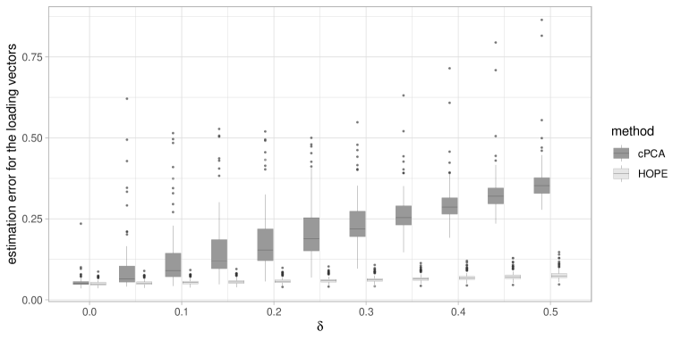
Figure 1: Boxplots of the estimation error over 100 replications under experiment configuration I with different $\delta$.

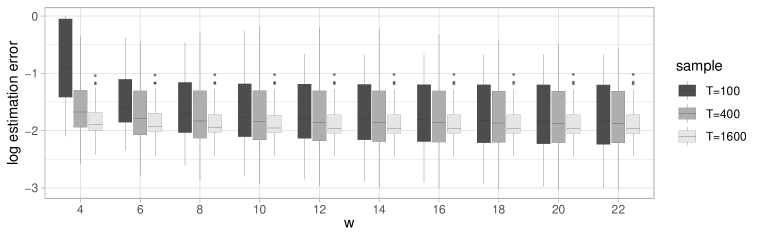
Figure 2: Boxplots of the logarithm of the estimation error for cPCA under experiment configuration II.

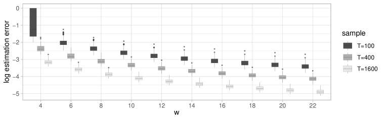
Figure 3: Boxplots of the logarithm of the estimation error for HOPE under experiment configuration II.

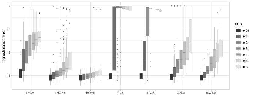
Figure 4: Boxplots of the logarithm of the estimation error under experiment configuration III. Seven methods with seven choices of $\delta$ are considered in total.

The experiment of Configuration II is conducted to verify the theoretical bounds on different sample sizes $T$ and signal strengths $w$. Figures 2 and 3 show the logarithm of the estimation errors under different ($w,T$) combinations. It can be seen from Figure 2 that the estimation error of cPCA decreases to a lower bound as $w$ and $T$ increases. The lower bound is associated with the bias term in (18) that cannot be reduced by a larger $w$ and $T$. This is the baseline error due to the non-orthogonality. In contrast, the phenomenon of HOPE is very different. Figure 3 shows that the performance improves monotonically as $w$ or $T$ increases. Again, this is consistent with the theoretical bounds in (26).

Figure 4 shows the boxplots of the logarithm of the estimation errors for 7 different methods with choices of $\delta$ under configuration III. ALS and OALS are implemented with $L=200$ random initiations. It can be seen that HOPE outperforms all the other methods. Again, the choice of $\delta$ does not affect the performance of HOPE significantly. One-step method (1HOPE) is better than the cPCA alone, and the iterative method HOPE is in turn better than the one-step method. When the coherence $\delta$ decreases, all methods perform better, but the advantage of HOPE over one-step method and the advantage of one-step method over the cPCA initialization become smaller. For the extremely small $\delta=0.01$, all loading vectors are almost orthogonal to each other. In this case, all the iterative procedures, including the one-step HOPE, perform similarly. In addition, ALS and cALS are always the worst under the cases $\delta\geq 0.1$. The hybrid methods cALS and cOALS improve the original randomized initialized ALS and OALS significantly, showing the advantages of the cPCA initialization. It is worth noting that cOALS has comparable performance with 1HOPE and HOPE when $\delta$ is small.

6 Applications

In this section, we demonstrate the use of TFM-cp model using the taxi traffic data set used in Chen et al., (2021). The data set was collected by the Taxi & Limousine Commission of New York City, and published at https://www1.nyc.gov/site/tlc/about/tlc-trip-record-data.page. Within Manhattan Island, it contains 69 predefined pick-up and drop-off zones and 24 hourly period for each day from January 1, 2009 to December 31, 2017. The total number of rides moving among the zones within each hour is recorded, yielding a ${\cal X}_{t}\in\mathbb{R}^{69\times 69\times 24}$ tensor for each day, using the hour of day as the third dimension due to the persistent daily pattern. We study business day and non-business day separately and ignore the gaps created by the separation. The length of the business-day series is 2,262, and that of the non-business-day is 1,025.

After some exploratory analysis, we decide to use the TFM-cp with $r=4$ factors for both series and estimate the model with $h=1$. For the non-business-day series, TFM-cp explains 66.2% of the variability in the data. In comparison, treating the tensor time series as a $114,264$ dimensional vector time series, the traditional vector factor model with 4 factors explains about 90.0% variability, but uses $4\times 114,264$ parameters for the loading matrix. Chen et al., (2021) used TFM-tucker with $4\times 4\times 4$ core factor tensor process. Using iTIPUP estimator of Han et al., 2020a , TFM-tucker explains 80.1% variability, but uses $1,536$ factors. Similarly, for the business-day series, the explained fractions of variability by the TFM-cp, vector factor model with 4 factors, and TFM-tucker with $4\times 4\times 4$ core factor tensor are 69.1%, 90.9%, 84.0%, respectively.

Figures 5 and 6 show the heatmap of the estimated loading vectors $({\mbox{\boldmath$a$}}_{11},\ldots,{\mbox{\boldmath$a$}}_{14})$ (related to pick-up locations) and $({\mbox{\boldmath$a$}}_{21},\ldots,{\mbox{\boldmath$a$}}_{24})$ (related to drop-off locations) of the 69 zones in Manhattan, respectively, for the business-day series. Table 1 shows the corresponding loading vectors $({\mbox{\boldmath$a$}}_{31},\ldots,{\mbox{\boldmath$a$}}_{34})$ (on the time of day dimension). It is seen that Factor 1 roughly corresponds to the morning rush hours of 6am to 11am, by the loading vector ${\mbox{\boldmath$a$}}_{31}$, with main activities in the midtown area as the pick-up locations, and Times square and 5th Avenue as the drop-off locations. For Factors 2-4, the areas that load heavily on the factors for pick-up are quite similar to that for drop-off, i.e., upper east side (with affluent neighborhoods and museums) on Factor 2, upper west side (with affluent neighborhoods and performing arts) on Factor 3, and lower east side (historic district with art) on Factor 4. The conventional business hours are heavily and almost exclusively loaded on Factors 2 and 3. The night life hours from 6pm to 1am load on Factor 4.

For the non-business day series, the estimated loading vectors $({\mbox{\boldmath$a$}}_{11},\ldots,{\mbox{\boldmath$a$}}_{14})$ (related to pick-up locations), $({\mbox{\boldmath$a$}}_{21},\ldots,{\mbox{\boldmath$a$}}_{24})$ (related to drop-off locations), $({\mbox{\boldmath$a$}}_{31},\ldots,{\mbox{\boldmath$a$}}_{34})$ (on the hour of day dimensions) are showed in Figures 7, 8, and Table 2, respectively. The pick-up and drop-off locations that heavily load on Factors 1, 3, 4 are similar to that for Factors 3, 2, 4 in the business day series. The daytime hours load on Factors 1 and 3, and the night life hours from 12am to 4am load on Factor 4. As for the second factor, it loads heavily on midtown area for pick-up, on the lower west side near Chelsea (with many restaurants and bars) for drop-off, on the morning/afternoon hours between 8am to 4pm as the dominating periods.

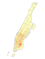
Figure 5: Loadings on four pickup factors for business day series

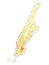
Figure 6: Loadings on four dropoff factors for business day series

0am		2		4		6		8		10		12pm		2		4		6		8		10		12am
1	1	1	1	1	2	10	42	56	45	36	24	18	15	12	11	9	7	7	8	8	6	5	3	2
2	3	1	1	1	0	2	6	19	27	24	25	27	30	27	30	31	25	27	29	25	17	13	10	6
3	6	3	2	1	1	2	6	12	19	17	20	22	24	24	27	29	26	31	36	34	25	20	16	11
4	21	14	9	6	4	2	4	6	9	12	12	13	14	14	15	15	13	19	28	35	37	37	36	34

Table 1: Estimated four loading vectors for hour of day fiber. Business day. Values are in percentage.

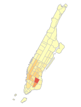
Figure 7: Loadings on four pickup factors for non-business day series

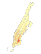
Figure 8: Loadings on four dropoff factors for non-business day series

0am		2		4		6		8		10		12pm		2		4		6		8		10		12am
1	13	9	6	4	2	1	2	5	11	19	25	27	29	29	29	28	26	27	31	29	22	20	17	13
2	12	11	9	7	5	5	11	18	30	39	40	39	31	25	23	20	16	16	16	11	6	5	6	8
3	8	5	3	2	2	1	2	6	11	19	26	30	33	33	33	33	29	28	27	22	17	13	11	8
4	39	40	38	29	14	4	3	3	5	7	10	12	14	16	16	15	14	16	19	21	21	21	22	23

Table 2: Estimated four loading vectors for hour of day fiber. Non-Business day. Values are in percentage.

We remark that this example is just for illustration and showcasing the interpretation of the proposed tensor factor model. We note that for the TFM-tucker model, one needs to identify a proper representation of the loading space in order to interpret the model. In Chen et al., (2021), varimax rotation was used to find the most sparse loading matrix representation to model interpretation. For TFM-cp, the model is unique hence interpretation can be made directly. Interpretation is impossible for the vector factor model in such a high dimensional case.

7 Discussion

In this paper, we propose a tensor factor model with a low rank CP structure and develop its corresponding estimation procedures. The estimation procedure takes advantage of the special structure of the model, resulting in faster convergence rate and more accurate estimations comparing to the standard procedures designed for the more general TFM-tucker, and the more general tensor CP decomposition. Numerical study illustrates the finite sample properties of the proposed estimators. The results show that HOPE uniformly outperforms the other methods, when observations follow the specified TFM-cp.

The HOPE in this paper is based on CP decomposition of the second moment tensor ${\mbox{\boldmath$\mathnormal{\Sigma}$}}_{h}=\sum_{i=1}^{r}\lambda_{i}(\otimes_{k=1}^{K}{\mbox{\boldmath$a$}}_{ik})^{\otimes 2}$, an order $2K$ tensor. The intuition that higher order tensors tend to have smaller coherence among the CP components leads to the consideration of using higher order cross-moments to have more orthogonal CP components. For example, let the $m$-th cross moment tensor with lags $0=h_{1}<\cdots<h_{m}$ be

$${\mbox{\boldmath$\mathnormal{\Sigma}$}}_{h_{1}...h_{m}}^{(m)}=\mathbb{E}\left[\otimes_{j=1}^{m}{\cal X}_{t-h_{j}}\right].$$

When the factor processes $f_{it}$, $i=1,\ldots,r$ are independent across different $i$ in TFM-cp, a naive 4-th cross moment tensor to estimate ${\mbox{\boldmath$a$}}_{ik}$ is

$${\mbox{\boldmath$\mathnormal{\Sigma}$}}_{h_{1}h_{2}h_{3}h_{4}}^{(4)}-{\mbox{\boldmath$\mathnormal{\Sigma}$}}_{h_{1}h_{2}}^{(2)}\otimes{\mbox{\boldmath$\mathnormal{\Sigma}$}}_{h_{3}h_{4}}^{(2)}-\mathbb{E}[{\cal X}_{t-h_{1}}\otimes{\cal X}^{*}_{t-h_{2}}\otimes{\cal X}_{t-h_{3}}\otimes{\cal X}_{t-h_{4}}^{*}]-\mathbb{E}[{\cal X}_{t-h_{1}}\otimes{\cal X}^{*}_{t-h_{2}}\otimes{\cal X}^{*}_{t-h_{3}}\otimes{\cal X}_{t-h_{4}}]$$

$$=\sum_{i=1}^{r}\lambda_{i,h_{1}h_{2}h_{3}h_{4}}^{(4)}(\otimes_{k=1}^{K}{\mbox{\boldmath$a$}}_{ik})^{\otimes 4},$$

with $\{{\cal X}_{t}^{*}\}$ being an independent coupled process of $\{{\cal X}_{t}\}$ and when $h_{j}=(j-1)h$,

$$\lambda_{i,h_{1}h_{2}h_{3}h_{4}}^{(4)} =\mathbb{E}\prod_{j=0}^{3}f_{i,t-jh}-[\mathbb{E}f_{i,t}f_{i,t-h}]^{2}-[\mathbb{E}f_{i,t}f_{i,t-2h}]^{2}-[\mathbb{E}f_{i,t}f_{i,t-h}][\mathbb{E}f_{i,t}f_{i,t-3h}].$$

This naive 4-th cross moment tensor has more orthogonal CP bases. In light tailed case, simulation shows that it is much worse than the second moment tensor, due to the reduced signal strength $\lambda_{i,h_{1}h_{2}h_{3}h_{4}}^{(4)}$. However, for heavy tailed and skewed data, this procedure would be helpful. It would be an interesting and challenging problem to develop an efficient higher cross moment tensor to improve the statistical and computational performance. We leave this for future research.

Supplementary Material to “CP Factor Model for Dynamic Tensors”

Yuefeng Han, Cun-Hui Zhang and Rong Chen

Rutgers University

Appendix A Proofs

A.1 Proofs of main theorems

Let $[n]$ denote the set $\{1,2,\ldots,n\}$. For a matrix $A=(a_{ij})\in\mathbb{R}^{m\times n}$, write the SVD as $A=U\Sigma V^{\top}$, where $\Sigma=\text{diag}(\sigma_{1}(A),\sigma_{2}(A),...,\sigma_{\min\{m,n\}}(A))$, with the singular values $\sigma_{1}(A)\geq\sigma_{2}(A)\geq\cdots\geq\sigma_{\min\{m,n\}}(A)\geq 0$ in descending order. For nonempty $J\subseteq[K]$, $\text{mat}_{J}({\cal A})$ is the mode $J$ matrix unfolding which maps ${\cal A}$ to $m_{J}\times m_{-J}$ matrix with $m_{J}=\prod_{j\in J}m_{j}$ and $m_{-J}=m/m_{J}$, e.g. $\text{mat}_{\{1,2\}}({\cal A})=\text{mat}_{3}^{\top}({\cal A})$ for $K=3$. Denote $a\wedge b=\min\{a,b\}$ and $a\vee b=\max\{a,b\}$.

Proof of Proposition 1.

Recall that ${\mbox{\boldmath$A$}}=({\mbox{\boldmath$a$}}_{1},...,{\mbox{\boldmath$a$}}_{r})\in\mathbb{R}^{d\times r}$, $\delta=\|{\mbox{\boldmath$A$}}^{\top}{\mbox{\boldmath$A$}}-I_{r}\|_{\rm S}$ and $\delta_{k}=\|{\mbox{\boldmath$A$}}_{k}^{\top}{\mbox{\boldmath$A$}}_{k}-I_{r}\|_{\rm S}$. Because ${\mbox{\boldmath$A$}}^{\top}{\mbox{\boldmath$A$}}=({\mbox{\boldmath$A$}}_{1}^{\top}{\mbox{\boldmath$A$}}_{1})\circ\cdots\circ({\mbox{\boldmath$A$}}_{K}^{\top}{\mbox{\boldmath$A$}}_{K})$ is the Hadamard product of correlation matrices, the spectrum of ${\mbox{\boldmath$A$}}^{\top}{\mbox{\boldmath$A$}}$ is contained inside the spectrum limits of ${\mbox{\boldmath$A$}}_{k}^{\top}{\mbox{\boldmath$A$}}_{k}$ for each $k$, so that

$$\delta\leq\min_{1\leq k\leq K}\delta_{k}.$$

Because ${\mbox{\boldmath$A$}}^{\top}{\mbox{\boldmath$A$}}-I_{r}$ is symmetric, its spectrum norm is bounded by its $\ell_{1}$ norm,

$$\delta\leq\max_{j\leq r}\sum_{i\neq j}|{\mbox{\boldmath$a$}}_{i}^{\top}{\mbox{\boldmath$a$}}_{j}|\leq(r-1)\vartheta\leq(r-1)\prod_{k=1}^{K}\vartheta_{k}$$

due to $|{\mbox{\boldmath$a$}}_{i}^{\top}{\mbox{\boldmath$a$}}_{j}|=\prod_{k=1}^{K}|{\mbox{\boldmath$a$}}_{ik}^{\top}{\mbox{\boldmath$a$}}_{jk}|=\prod_{k=1}^{K}|\sigma_{ij,k}|$. Moreover, for any $j\leq r$ and $1\leq k_{1}<k_{2}\leq K$,

$$\sum_{i\neq j}\prod_{k=1}^{K}|\sigma_{ij,k}| \leq\sum_{i\neq j}|\sigma_{ij,k_{1}}\sigma_{ij,k_{2}}|\,\max_{i\neq j}\prod_{k\neq k_{1},k\neq k_{2}}|\sigma_{ij,k}|$$

$$\leq\Big{(}\prod_{k=1}^{K}\eta_{jk}\Big{)}r^{-(K-2)/2}\,\max_{i\neq j}\prod_{k\neq k_{1},k\neq k_{2}}\sqrt{r}|\sigma_{ij,k}|/\eta_{jk}$$

as $\eta_{jk}=(\sum_{i\neq j}\sigma_{ij,k}^{2})^{1/2}$. The proof is complete as $k_{1}$ and $k_{2}$ are arbitrary. ∎

Proof of Theorem 1.

Recall $\widehat{\mbox{\boldmath$\mathnormal{\Sigma}$}}_{h}=\sum_{t=h+1}^{T}{\cal X}_{t-h}\otimes{\cal X}_{t}$, $\lambda_{i}=w_{i}^{2}\cdot\mathbb{E}f_{i,t-h}f_{i,t}$, ${\mbox{\boldmath$a$}}_{i}=\hbox{\rm vec}({\mbox{\boldmath$a$}}_{i1}\otimes{\mbox{\boldmath$a$}}_{i2}\otimes\cdots\otimes{\mbox{\boldmath$a$}}_{iK})$, $d=d_{1}d_{2}...d_{K}$. Let $e_{t}=\hbox{\rm vec}({\cal E}_{t})$. Write

$$\widetilde{\mbox{\boldmath$\mathnormal{\Sigma}$}}:=\hbox{\rm mat}_{[K]}\big{(}\widehat{\mbox{\boldmath$\mathnormal{\Sigma}$}}_{h}\big{)}=\sum_{i=1}^{r}\lambda_{i}{\mbox{\boldmath$a$}}_{i}{\mbox{\boldmath$a$}}_{i}^{\top}+{\mbox{\boldmath$\mathnormal{\Psi}$}}^{*}={\mbox{\boldmath$A$}}{\mbox{\boldmath$\mathnormal{\Lambda}$}}{\mbox{\boldmath$A$}}^{\top}+{\mbox{\boldmath$\mathnormal{\Psi}$}}^{*},$$

where ${\mbox{\boldmath$\mathnormal{\Lambda}$}}=\text{diag}(\lambda_{1},...,\lambda_{r})$. Assume $A$ has SVD ${\mbox{\boldmath$A$}}=\widetilde{U}\widetilde{D}\widetilde{V}^{\top}$, with $\widetilde{D}=\text{diag}(\widetilde{\sigma}_{1},...,\widetilde{\sigma}_{r})$. Let ${\mbox{\boldmath$U$}}=\widetilde{U}\widetilde{V}^{\top}=({\mbox{\boldmath$u$}}_{1},...,{\mbox{\boldmath$u$}}_{r})$. Then, ${\mbox{\boldmath$U$}}^{\top}{\mbox{\boldmath$U$}}={\mbox{\boldmath$I$}}_{r}$. Note that $\widetilde{\mbox{\boldmath$\mathnormal{\Sigma}$}}/2+\widetilde{\mbox{\boldmath$\mathnormal{\Sigma}$}}^{\top}/2$ is guaranteed to be symmetric. Without loss of generality, assume $\widetilde{\mbox{\boldmath$\mathnormal{\Sigma}$}}$ is symmetric.

By (8), $\|{\mbox{\boldmath$A$}}^{\top}{\mbox{\boldmath$A$}}-{\mbox{\boldmath$I$}}_{r}\|_{\rm S}=\|\widetilde{D}^{2}-{\mbox{\boldmath$I$}}_{r}\|_{\rm S}\leq\delta$. It follows that $\max_{1\leq i\leq r}|\widetilde{\sigma}_{i}^{2}-1|\leq\delta$. As $\delta<1$, basic calculation shows that $\max_{i}|\widetilde{\sigma}_{i}-1|\leq\delta/(2-\delta)$. Thus,

$$\|{\mbox{\boldmath$A$}}-{\mbox{\boldmath$U$}}\|_{\rm S}=\|\widetilde{D}-{\mbox{\boldmath$I$}}_{r}\|_{\rm S}\leq\delta/(2-\delta)<\delta<1.$$

This yields

$$\max_{i}\|{\mbox{\boldmath$a$}}_{i}-{\mbox{\boldmath$u$}}_{i}\|_{2}\leq\delta<1.$$

It follows that $\max_{i}(2-2{\mbox{\boldmath$a$}}_{i}^{\top}{\mbox{\boldmath$u$}}_{i})\leq\delta^{2}$. Since $1-x^{2}\leq 2-2x$, we have

$$\|{\mbox{\boldmath$a$}}_{i}{\mbox{\boldmath$a$}}_{i}^{\top}-{\mbox{\boldmath$u$}}_{i}{\mbox{\boldmath$u$}}_{i}^{\top}\|_{\rm S}=\sqrt{1-({\mbox{\boldmath$a$}}_{i}^{\top}{\mbox{\boldmath$u$}}_{i})^{2}}\leq\sqrt{2-2({\mbox{\boldmath$a$}}_{i}^{\top}{\mbox{\boldmath$u$}}_{i})}\leq\delta<1.$$ (31)

Let the top $r$ eigenvectors of $\widetilde{\mbox{\boldmath$\mathnormal{\Sigma}$}}$ be $\widehat{\mbox{\boldmath$U$}}=(\widehat{\mbox{\boldmath$u$}}_{1},...,\widehat{\mbox{\boldmath$u$}}_{r})\in\mathbb{R}^{d\times r}$. Note that $\lambda_{1}>\lambda_{2}>...>\lambda_{r}>\lambda_{r+1}=0$. By Wedin’s perturbation theorem (Wedin,, 1972) and Lemma 2, for any $1\leq i\leq r$,

$$\|\widehat{\mbox{\boldmath$u$}}_{i}\widehat{\mbox{\boldmath$u$}}_{i}^{\top}-{\mbox{\boldmath$u$}}_{i}{\mbox{\boldmath$u$}}_{i}^{\top}\|_{\rm S}\leq\frac{2\|{\mbox{\boldmath$A$}}{\mbox{\boldmath$\mathnormal{\Lambda}$}}{\mbox{\boldmath$A$}}^{\top}-{\mbox{\boldmath$U$}}{\mbox{\boldmath$\mathnormal{\Lambda}$}}{\mbox{\boldmath$U$}}^{\top}+{\mbox{\boldmath$\mathnormal{\Psi}$}}^{*}\|_{\rm S}}{\min\{\lambda_{i-1}-\lambda_{i},\lambda_{i}-\lambda_{i+1}\}}\leq\frac{2\lambda_{1}\delta+2\|{\mbox{\boldmath$\mathnormal{\Psi}$}}^{*}\|_{\rm S}}{\min\{\lambda_{i-1}-\lambda_{i},\lambda_{i}-\lambda_{i+1}\}}.$$ (32)

Combining (31) and (32), we have

$$\|\widehat{\mbox{\boldmath$u$}}_{i}\widehat{\mbox{\boldmath$u$}}_{i}^{\top}-{\mbox{\boldmath$a$}}_{i}{\mbox{\boldmath$a$}}_{i}^{\top}\|_{\rm S} \leq\delta+\frac{2\lambda_{1}\delta+2\|{\mbox{\boldmath$\mathnormal{\Psi}$}}^{*}\|_{\rm S}}{\min\{\lambda_{i-1}-\lambda_{i},\lambda_{i}-\lambda_{i+1}\}}.$$ (33)

We formulate each $\widehat{\mbox{\boldmath$u$}}_{i}\in\mathbb{R}^{d}$ to be a $K$-way tensor $\widehat{\mbox{\boldmath$U$}}_{i}\in\mathbb{R}^{d_{1}\times\cdots\times d_{K}}$. Let $\widehat{\mbox{\boldmath$U$}}_{ik}=\hbox{\rm mat}_{k}(\widehat{\mbox{\boldmath$U$}}_{i})$, which is viewed as an estimate of ${\mbox{\boldmath$a$}}_{ik}\hbox{\rm vec}(\otimes_{\ell\neq k}^{K}{\mbox{\boldmath$a$}}_{i\ell})^{\top}\in\mathbb{R}^{d_{k}\times(d/d_{k})}$. Then $\widehat{\mbox{\boldmath$a$}}^{{\rm\tiny cpca}}_{ik}$ is the top left singular vector of $\widehat{\mbox{\boldmath$U$}}_{ik}$. By Lemma 3,

$$\|\widehat{\mbox{\boldmath$a$}}^{{\rm\tiny cpca}}_{ik}\widehat{\mbox{\boldmath$a$}}^{{\rm\tiny cpca}\top}_{ik}-{\mbox{\boldmath$a$}}_{ik}{\mbox{\boldmath$a$}}_{ik}^{\top}\|_{\rm S}^{2}\wedge(1/2)\leq\|\widehat{\mbox{\boldmath$u$}}_{i}\widehat{\mbox{\boldmath$u$}}_{i}^{\top}-{\mbox{\boldmath$a$}}_{i}{\mbox{\boldmath$a$}}_{i}^{\top}\|_{\rm S}^{2}.$$ (34)

Substituting (33) and Lemma 1 into the above equation, since $\|{\mbox{\boldmath$\mathnormal{\Psi}$}}^{*}\|_{\rm S}/\min\{\lambda_{i-1}-\lambda_{i},\lambda_{i}-\lambda_{i+1}\}\lesssim 1$, we have the desired results. ∎

Lemma 1.

Suppose Assumptions 1, 2 hold and $\delta<1$. Let $\widetilde{\mbox{\boldmath$\mathnormal{\Sigma}$}}=\sum_{i=1}^{r}\lambda_{i}{\mbox{\boldmath$a$}}_{i}{\mbox{\boldmath$a$}}_{i}^{\top}+{\mbox{\boldmath$\mathnormal{\Psi}$}}^{*}$ and $1/\gamma=1/\gamma_{1}+2/\gamma_{2}$. In an event with probability at least $1-(Tr)^{-c}/2-e^{-d}/6$, we have

$$\|{\mbox{\boldmath$\mathnormal{\Psi}$}}^{*}\|_{\rm S} \leq C\max_{1\leq i\leq r}w_{i}^{2}\left(\sqrt{\frac{r+\log T}{T}}+\frac{(r+\log T)^{1/\gamma}}{T}\right)+\frac{C\sigma^{2}(d+\sqrt{dT})}{T}$$

$$\qquad\quad+C\sigma\max_{1\leq i\leq r}w_{i}\sqrt{\frac{d}{T}}.$$ (35)

Proof.

Let $\Upsilon_{0}=T^{-1}\sum_{t=1}^{T}\sum_{i,j=1}^{r}w_{i}w_{j}f_{it}f_{jt}{\mbox{\boldmath$a$}}_{i}{\mbox{\boldmath$a$}}_{j}^{\top}$, $\overline{\mathbb{E}}(\cdot)=\mathbb{E}(\cdot|f_{it},1\leq i\leq r,1\leq t\leq T)$. Define $e_{t}=\hbox{\rm vec}({\cal E}_{t})$. Write

$$\widetilde{\mbox{\boldmath$\mathnormal{\Sigma}$}} =\frac{1}{T-h}\sum_{t=h+1}^{T}\hbox{\rm vec}({\cal X}_{t-h})\hbox{\rm vec}({\cal X}_{t})^{\top}$$

$$=\sum_{i=1}^{r}\lambda_{i}{\mbox{\boldmath$a$}}_{i}{\mbox{\boldmath$a$}}_{i}^{\top}+\sum_{i,j=1}^{r}\frac{1}{T-h}\sum_{t=h+1}^{T}w_{i}w_{j}\left(f_{i,t-h}f_{j,t}-\mathbb{E}f_{i,t-h}f_{j,t}\right){\mbox{\boldmath$a$}}_{i}{\mbox{\boldmath$a$}}_{j}^{\top}+\frac{1}{T-h}\sum_{t=h+1}^{T}e_{t-h}e_{t}^{\top}$$

$$\quad+\frac{1}{T-h}\sum_{t=h+1}^{T}\sum_{i=1}^{r}w_{i}f_{i,t-h}{\mbox{\boldmath$a$}}_{i}e_{t}^{\top}+\frac{1}{T-h}\sum_{t=h+1}^{T}\sum_{i=1}^{r}w_{i}f_{i,t}e_{t-h}{\mbox{\boldmath$a$}}_{i}^{\top}$$

$$:=\sum_{i=1}^{r}\lambda_{i}{\mbox{\boldmath$a$}}_{i}{\mbox{\boldmath$a$}}_{i}^{\top}+\Delta_{1}+\Delta_{2}+\Delta_{3}+\Delta_{4}.$$

That is, ${\mbox{\boldmath$\mathnormal{\Psi}$}}^{*}=\Delta_{1}+\Delta_{2}+\Delta_{3}+\Delta_{4}$.

We first bound $\|\Delta_{1}\|_{\rm S}$. Let

$$\Theta_{h}=\sum_{t=h+1}^{T}\begin{pmatrix}f_{1,t-h}f_{1,t}&f_{1,t-h}f_{2,t}&\cdots&f_{1,t-h}f_{r,t}\\ \vdots&\vdots&\ddots&\vdots\\ f_{r,t-h}f_{1,t}&f_{r,t-h}f_{2,t}&\cdots&f_{r,t-h}f_{r,t}\end{pmatrix}.$$ (36)

Then

$$\Delta_{1}=(w_{1}{\mbox{\boldmath$a$}}_{1},...,w_{r}{\mbox{\boldmath$a$}}_{r})\left(\frac{\Theta_{h}-\mathbb{E}\Theta_{h}}{T-h}\right)(w_{1}{\mbox{\boldmath$a$}}_{1},...,w_{r}{\mbox{\boldmath$a$}}_{r})^{\top}.$$

For any unit vector $u$ in $\mathbb{R}^{r}$, there exist $u_{j}\in\mathbb{R}^{r}$ with $\|u_{j}\|_{2}\leq 1$, $j=1,...,N_{r,\epsilon}$ such that $\max_{\|u\|_{2}\leq 1}\min_{1\leq j\leq N_{r,\epsilon}}\|u-u_{j}\|_{2}\leq\epsilon$. The standard volume comparison argument implies that the covering number $N_{r,\epsilon}=\lfloor(1+2/\epsilon)^{r}\rfloor$. Then, there exist $u_{j},v_{j^{\prime}}\in\mathbb{R}^{r}$, $1\leq j,j^{\prime}\leq N_{r,1/3}:=7^{r}$, such that $\|u_{j}\|_{2}=\|v_{j^{\prime}}\|_{2}=1$ and

$$\|\Theta_{h}-\mathbb{E}\Theta_{h}\|_{\rm S}-\max_{1\leq j,j^{\prime}\leq N_{r,1/3}}\left|u_{j}^{\top}(\Theta_{h}-\mathbb{E}\Theta_{h})v_{j}\right|\leq(2/3)\|\Theta_{h}-\mathbb{E}\Theta_{h}\|_{\rm S}.$$

It follows that

$$\|\Theta_{h}-\mathbb{E}\Theta_{h}\|_{\rm S}\leq 3\max_{1\leq j,j^{\prime}\leq N_{r,1/3}}\left|u_{j}^{\top}(\Theta_{h}-\mathbb{E}\Theta_{h})v_{j}\right|.$$

As $1/\gamma=1/\gamma_{1}+2/\gamma_{2}$, by Theorem 1 in Merlevède et al., (2011),

$$\mathbb{P}\left(\left|u_{j}^{\top}(\Theta_{h}-\mathbb{E}\Theta_{h})v_{j}\right|\geq x\right) \leq T\exp\left(-\frac{x^{\gamma}}{c_{1}}\right)+\exp\left(-\frac{x^{2}}{c_{2}T}\right)$$

$$\quad+\exp\left(-\frac{x^{2}}{c_{3}T}\exp\left(\frac{x^{\gamma(1-\gamma)}}{c_{4}(\log x)^{\gamma}}\right)\right).$$ (37)

Hence,

$$\mathbb{P}\left(\left\|\Theta_{h}-\mathbb{E}\Theta_{h}\right\|_{\rm S}/3\geq x\right) \leq N_{r,1/3}^{2}T\exp\left(-\frac{x^{\gamma}}{c_{1}}\right)+N_{r,1/3}^{2}\exp\left(-\frac{x^{2}}{c_{2}T}\right)$$

$$\quad+N_{r,1/3}^{2}\exp\left(-\frac{x^{2}}{c_{3}T}\exp\left(\frac{x^{\gamma(1-\gamma)}}{c_{4}(\log x)^{\gamma}}\right)\right).$$

As $h$ is fixed and $T\geq 4h$, choosing $x\asymp\sqrt{T(r+\log T)}+(r+\log T)^{1/\gamma}$, in an event $\Omega_{1}$ with probability at least $1-(Tr)^{-C_{1}}/2$,

$$\left\|\frac{\Theta_{h}-\mathbb{E}\Theta_{h}}{T-h}\right\|_{\rm S}\leq C\sqrt{\frac{r+\log(T)}{T}}+\frac{C(r+\log T)^{1/\gamma}}{T}.$$

It follows that, in the event $\Omega_{1}$,

$$\|\Delta_{1}\|_{\rm S} \leq\|{\mbox{\boldmath$A$}}\|_{\rm S}^{2}\max_{1\leq i\leq r}w_{i}^{2}\cdot\left\|\frac{\Theta_{h}-\mathbb{E}\Theta_{h}}{T-h}\right\|_{\rm S}$$

$$\leq C\max_{1\leq i\leq r}w_{i}^{2}\left(\sqrt{\frac{r+\log T}{T}}+\frac{(r+\log T)^{1/\gamma}}{T}\right),$$

and, as $\mathbb{E}f_{i,t}^{2}=1$,

$$\|\Upsilon_{0}\|_{\rm S} \leq\Big{\|}\sum_{i=1}^{r}w_{i}^{2}{\mbox{\boldmath$a$}}_{i}{\mbox{\boldmath$a$}}_{j}^{\top}\Big{\|}_{\rm S}+\Big{\|}\frac{1}{T}\sum_{t=1}^{T}\sum_{i,j=1}^{r}w_{i}w_{j}(f_{i,t}f_{j,t}-\mathbb{E}f_{i,t}f_{j,t}){\mbox{\boldmath$a$}}_{i}{\mbox{\boldmath$a$}}_{j}^{\top}\Big{\|}_{\rm S}$$

$$\leq\|{\mbox{\boldmath$A$}}\|_{\rm S}^{2}\max_{1\leq i\leq r}w_{i}^{2}+\Big{\|}\frac{1}{T}\sum_{t=1}^{T}\sum_{i,j=1}^{r}w_{i}w_{j}(f_{i,t}f_{j,t}-\mathbb{E}f_{i,t}f_{j,t}){\mbox{\boldmath$a$}}_{i}{\mbox{\boldmath$a$}}_{j}^{\top}\Big{\|}_{\rm S}$$

$$\leq(1+\delta)^{2}\max_{1\leq i\leq r}w_{i}^{2}+C\max_{1\leq i\leq r}w_{i}^{2}\left(\sqrt{\frac{r+\log T}{T}}+\frac{(r+\log T)^{1/\gamma}}{T}\right)$$ (38)

$$:=\Delta_{\Upsilon}.$$

Note that $\Delta_{\Upsilon}\lesssim\max_{1\leq i\leq r}w_{i}^{2}.$

For $\|\Delta_{2}\|_{\rm S}$, we split the sum into two terms over the index sets, $S_{1}=\{(h,2h]\cup(3h,4h]\cup\cdots\}\cap(h,T]$ and its complement $S_{2}$ in $(h,T]$, so that $\{e_{t-h},t\in S_{a}\}$ is independent of $\{e_{t},t\in S_{a}\}$ for each $a=1,2$. Let $n_{a}=|S_{a}|$. By Lemma 5(i),

$$\mathbb{P}\left(\left\|\sum_{t\in S_{a}}e_{t-h}e_{t}^{\top}\right\|_{\rm S}\geq\sigma^{2}(d+2\sqrt{dn_{a}})+\sigma^{2}x(x+2\sqrt{n_{a}}+2\sqrt{d})\right)\leq 2e^{-\frac{x^{2}}{2}}.$$

With $x\asymp\sqrt{d}$, in an event $\Omega_{2}$ with probability at least $1-e^{-d}/18$,

$$\|\Delta_{2}\|_{\rm S} \leq\sum_{a=1,2}\left\|\sum_{t\in S_{a}}\frac{e_{t-h}e_{t}^{\top}}{T-h}\right\|_{\rm S}\leq\frac{C\sigma^{2}(d+\sqrt{dT})}{T}.$$

For $\Delta_{3}$, by Assumption 1, for any $u$ and $v$ in $\mathbb{R}^{d}$ we have

$$\overline{\mathbb{E}}\left\{u^{\top}\left(\frac{1}{\sqrt{T}}\sum_{t=h+1}^{T}\sum_{i=1}^{r}w_{i}f_{i,t-h}{\mbox{\boldmath$a$}}_{i}e_{t}^{\top}\right)v\right\}^{2}\leq\sigma^{2}\|\Upsilon_{0}\|_{\rm S}\|u\|_{2}^{2}\|v\|_{2}^{2}.$$

Thus for vectors $u_{i}$ and $v_{i}$ with $\|u_{i}\|_{2}=\|v_{i}\|_{2}=1$, $i=1,2$,

$$\sigma^{-2}\|\Upsilon_{0}\|_{\rm S}^{-1}\overline{\mathbb{E}}\left(u_{1}^{\top}\left(\frac{1}{\sqrt{T}}\sum_{t=h+1}^{T}\sum_{i=1}^{r}w_{i}f_{i,t-h}{\mbox{\boldmath$a$}}_{i}e_{t}^{\top}\right)v_{1}-u_{2}^{\top}\left(\frac{1}{\sqrt{T}}\sum_{t=h+1}^{T}\sum_{i=1}^{r}w_{i}f_{i,t-h}{\mbox{\boldmath$a$}}_{i}e_{t}^{\top}\right)v_{2}\right)^{2}$$

$$\leq\left(\|u_{1}-u_{2}\|_{2}\|v_{1}\|_{2}+\|u_{2}\|_{2}\|v_{1}-v_{2}\|_{2}\right)^{2}$$

$$\leq 2\left(\|u_{1}-u_{2}\|_{2}^{2}+\|v_{1}-v_{2}\|_{2}^{2}\right)$$

$$=2\mathbb{E}\{(u_{1}-u_{2})^{\top}\xi+(v_{1}-v_{2})^{\top}\zeta\}^{2},$$

where $\xi$ and $\zeta$ are iid $N(0,I_{d})$ vectors. The Sudakov- Fernique inequality yields

$$\sigma^{-2}\|\Upsilon_{0}\|_{\rm S}^{-1}\overline{\mathbb{E}}\left\|\frac{1}{\sqrt{T}}\sum_{t=h+1}^{T}\sum_{i=1}^{r}w_{i}f_{i,t-h}{\mbox{\boldmath$a$}}_{i}e_{t}^{\top}\right\|_{\rm S}\leq\sqrt{2}\mathbb{E}\sup_{\|u\|_{2}=\|v\|_{2}=1}\left|u^{\top}\xi+v^{\top}\zeta\right|\leq\sqrt{2}\mathbb{E}(\|\xi\|_{2}+\|\zeta\|_{2})$$

As $\mathbb{E}\|\xi\|_{2}=\mathbb{E}\|\zeta\|_{2}\leq\sqrt{d}$, it follows that

$$\overline{\mathbb{E}}\left\|\frac{1}{T-h}\sum_{t=h+1}^{T}\sum_{i=1}^{r}w_{i}f_{i,t-h}{\mbox{\boldmath$a$}}_{i}e_{t}^{\top}\right\|_{\rm S}\leq\frac{\sigma\sqrt{8Td}\|\Upsilon_{0}\|_{\rm S}^{1/2}}{T-h}.$$ (39)

Elementary calculation shows that, $\left\|\sum_{t=h+1}^{T}\sum_{i=1}^{r}w_{i}f_{i,t-h}{\mbox{\boldmath$a$}}_{i}e_{t}^{\top}\right\|_{\rm S}$ is a $\sigma\sqrt{T}\|\Upsilon_{0}\|_{\rm S}^{1/2}$ Lipschitz function. Then, by Gaussian concentration inequalities for Lipschitz functions,

$$\mathbb{P}\left(\left\|\frac{1}{T-h}\sum_{t=h+1}^{T}\sum_{i=1}^{r}w_{i}f_{i,t-h}{\mbox{\boldmath$a$}}_{i}e_{t}^{\top}\right\|_{\rm S}\geq\frac{\sigma\sqrt{8Td}}{T-h}\|\Upsilon_{0}\|_{\rm S}^{1/2}+\frac{\sigma\sqrt{T}}{T-h}\|\Upsilon_{0}\|_{\rm S}^{1/2}x\right)\leq 2e^{-\frac{x^{2}}{2}}.$$

With $x\asymp\sqrt{d}$, in an event $\Omega_{3}$ with probability at least $1-e^{-d}/18$,

$$\|\Delta_{3}\|_{\rm S}\leq C\sigma\sqrt{\frac{d}{T}}\|\Upsilon_{0}\|_{\rm S}^{1/2}.$$

Hence, in the event $\Omega_{1}\cap\Omega_{3}$,

$$\|\Delta_{3}\|_{\rm S}\leq C\sigma\sqrt{\frac{d}{T}}\Delta_{\Upsilon}^{1/2}.$$

Similarly, $\|\Delta_{4}\|_{\rm S}\leq C\sigma\sqrt{d/T}\Delta_{\Upsilon}^{1/2}$.

Therefore, in the event $\Omega_{1}\cap\Omega_{2}\cap\Omega_{3}$ with probability at least $1-(Tr)^{-c}/2-e^{-d}/6$,

$$\|{\mbox{\boldmath$\mathnormal{\Psi}$}}^{*}\|_{\rm S} \leq C\max_{1\leq i\leq r}w_{i}^{2}\left(\sqrt{\frac{r+\log T}{T}}+\frac{(r+\log T)^{1/\gamma}}{T}\right)+\frac{C\sigma^{2}(d+\sqrt{dT})}{T}$$

$$\qquad\quad+C\max_{1\leq i\leq r}w_{i}\sigma\sqrt{\frac{d}{T}}.$$

∎

Proof of Theorem 2.

Recall $\widehat{\mbox{\boldmath$A$}}_{k}^{(m)}=(\widehat{\mbox{\boldmath$a$}}_{1k}^{(m)},\ldots,\widehat{\mbox{\boldmath$a$}}_{rk}^{(m)})\in\mathbb{R}^{d_{k}\times r}$, $\widehat{\Sigma}_{k}^{(m)}=\widehat{\mbox{\boldmath$A$}}_{k}^{(m)\top}\widehat{\mbox{\boldmath$A$}}_{k}^{(m)}$, and $\widehat{\mbox{\boldmath$B$}}_{k}^{(m)}=\widehat{\mbox{\boldmath$A$}}_{k}^{(m)}(\widehat{\Sigma}_{k}^{(m)})^{-1}=(\widehat{\mbox{\boldmath$b$}}_{1k}^{(m)},...,\widehat{\mbox{\boldmath$b$}}_{rk}^{(m)})\in\mathbb{R}^{d_{k}\times r}$. Let $\overline{\mathbb{E}}(\cdot)=\mathbb{E}(\cdot|f_{it},1\leq i\leq r,1\leq t\leq T)$ and $\overline{\mathbb{P}}(\cdot)=\mathbb{P}(\cdot|f_{it},1\leq i\leq r,1\leq t\leq T)$. Also let

$$\widebar{\lambda}_{i}=\frac{1}{T-h}\sum_{t=h+1}^{T}w_{i}^{2}f_{i,t-h}f_{i,t}.$$

Without loss of generality, assume $\widehat{\mbox{\boldmath$\mathnormal{\Sigma}$}}_{h}$ is symmetric. Write

$$\widehat{\mbox{\boldmath$\mathnormal{\Sigma}$}}_{h} =\frac{1}{T-h}\sum_{t=h+1}^{T}{\cal X}_{t-h}\otimes{\cal X}_{t}$$

$$=\sum_{i=1}^{r}\widebar{\lambda}_{i}\otimes_{k=1}^{2K}{\mbox{\boldmath$a$}}_{ik}+\sum_{i\neq j}^{r}\frac{1}{T-h}\sum_{t=h+1}^{T}w_{i}w_{j}f_{i,t-h}f_{j,t}\otimes_{k=1}^{K}{\mbox{\boldmath$a$}}_{ik}\otimes_{k=K+1}^{2K}{\mbox{\boldmath$a$}}_{jk}$$

$$\quad+\frac{1}{T-h}\sum_{t=h+1}^{T}\sum_{i=1}^{r}w_{i}f_{i,t-h}\otimes_{k=1}^{K}{\mbox{\boldmath$a$}}_{ik}\otimes{\cal E}_{t}+\frac{1}{T-h}\sum_{t=h+1}^{T}\sum_{i=1}^{r}w_{i}f_{i,t}{\cal E}_{t-h}\otimes_{k=K+1}^{2K}{\mbox{\boldmath$a$}}_{ik}$$

$$\quad+\frac{1}{T-h}\sum_{t=h+1}^{T}{\cal E}_{t-h}\otimes{\cal E}_{t}$$

$$:=\sum_{i=1}^{r}\widebar{\lambda}_{i}\otimes_{k=1}^{2K}{\mbox{\boldmath$a$}}_{ik}+\Delta_{1}+\Delta_{2}+\Delta_{3}+\Delta_{4},$$ (40)

with ${\mbox{\boldmath$a$}}_{i,K+k}={\mbox{\boldmath$a$}}_{ik}$ for all $1\leq k\leq K$. Let ${\mbox{\boldmath$\mathnormal{\Psi}$}}=\Delta_{1}+\Delta_{2}+\Delta_{3}+\Delta_{4}$.

By Theorem 1, in an event $\Omega_{0}$ with probability at least $1-(Tr)^{-c}/2-e^{-d}/6$,

$$\|\widehat{\mbox{\boldmath$a$}}_{ik}^{(0)}\widehat{\mbox{\boldmath$a$}}_{ik}^{(0)\top}-{\mbox{\boldmath$a$}}_{ik}{\mbox{\boldmath$a$}}_{ik}^{\top}\|_{\rm S} \leq\delta+\frac{2\lambda_{1}\delta+C_{1}R^{(0)}}{\min\{\lambda_{i-1}-\lambda_{i},\lambda_{i}-\lambda_{i+1}\}},$$

where

$$R^{(0)} =\max_{1\leq i\leq r}w_{i}^{2}\left(\sqrt{\frac{r+\log T}{T}}+\frac{(r+\log T)^{1/\gamma}}{T}\right)+\frac{\sigma^{2}(d+\sqrt{dT})}{T}+\sigma\max_{1\leq i\leq r}w_{i}\sqrt{\frac{d}{T}}.$$

Then in the event $\Omega_{0}$,

$$\psi_{0}:=\max_{i}\max_{k}\|\widehat{\mbox{\boldmath$a$}}_{ik}^{(0)}\widehat{\mbox{\boldmath$a$}}_{ik}^{(0)\top}-{\mbox{\boldmath$a$}}_{ik}{\mbox{\boldmath$a$}}_{ik}^{\top}\|_{\rm S}\leq\max_{i}\left(\frac{C_{1}^{\prime}\lambda_{1}\delta+C_{1}^{\prime}R^{(0)}}{\min\{\lambda_{i-1}-\lambda_{i},\lambda_{i}-\lambda_{i+1}\}}\right).$$ (41)

At $m$-th step, let

$$\psi_{m,k}:=\max_{i}\|\widehat{\mbox{\boldmath$a$}}_{ik}^{(m)}\widehat{\mbox{\boldmath$a$}}_{ik}^{(m)\top}-{\mbox{\boldmath$a$}}_{ik}{\mbox{\boldmath$a$}}_{ik}^{\top}\|_{\rm S},\qquad\psi_{m}=\max_{k}\psi_{m,k}.$$ (42)

Given $\widehat{\mbox{\boldmath$a$}}_{i\ell}^{(m)}$ ($1\leq i\leq r,1\leq\ell\leq K$), the $(m+1)$th iteration produces estimates $\widehat{\mbox{\boldmath$a$}}_{ik}^{(m+1)}$, which is the top left singular vector of $\widehat{\mbox{\boldmath$\mathnormal{\Sigma}$}}_{h}\times_{l\in[2K]\backslash\{k,K+k\}}\widehat{\mbox{\boldmath$b$}}_{il}^{(m)\top}$. Note that $\widehat{\mbox{\boldmath$\mathnormal{\Sigma}$}}_{h}=\sum_{j=1}^{r}\widebar{\lambda}_{j}\otimes_{\ell=1}^{2K}{\mbox{\boldmath$a$}}_{j\ell}+{\mbox{\boldmath$\mathnormal{\Psi}$}}$, with ${\mbox{\boldmath$a$}}_{j,\ell+K}={\mbox{\boldmath$a$}}_{j\ell}$. The “noiseless” version of this update is given by

$$\widehat{\mbox{\boldmath$\mathnormal{\Sigma}$}}_{h}\times_{l\in[2K]\backslash\{k,K+k\}}{\mbox{\boldmath$b$}}_{il}^{\top}=\widebar{\lambda}_{i}{\mbox{\boldmath$a$}}_{ik}{\mbox{\boldmath$a$}}_{ik}^{\top}+{\mbox{\boldmath$\mathnormal{\Psi}$}}\times_{l\in[2K]\backslash\{k,K+k\}}{\mbox{\boldmath$b$}}_{il}^{\top}.$$ (43)

At $(m+1)$-th iteration, for any $1\leq i\leq r$, we have

$$\widehat{\mbox{\boldmath$\mathnormal{\Sigma}$}}_{h}\times_{l\in[2K]\backslash\{k,K+k\}}\widehat{\mbox{\boldmath$b$}}_{il}^{(m)\top}=\sum_{j=1}^{r}\widetilde{\lambda}_{j,i}{\mbox{\boldmath$a$}}_{jk}{\mbox{\boldmath$a$}}_{jk}^{\top}+{\mbox{\boldmath$\mathnormal{\Psi}$}}\times_{l\in[2K]\backslash\{k,K+k\}}\widehat{\mbox{\boldmath$b$}}_{il}^{(m)\top},$$

where

$$\widetilde{\lambda}_{j,i}=\widebar{\lambda}_{j}\prod_{l\in[2K]\backslash\{k,K+k\}}{\mbox{\boldmath$a$}}_{jl}^{\top}\widehat{\mbox{\boldmath$b$}}_{il}^{(m)}.$$

Let

$$\lambda_{j,i} =\lambda_{j}\prod_{l\in[2K]\backslash\{k,K+k\}}{\mbox{\boldmath$a$}}_{jl}^{\top}\widehat{\mbox{\boldmath$b$}}_{il}^{(m)},$$

$$\phi_{m,k} =\frac{\sqrt{2}\psi_{m}}{(1-\delta_{k}-\|\widehat{\Sigma}_{k}^{(m)}-\Sigma_{k}\|_{\rm S})^{1/2}},$$

$$\phi_{m} =\max_{k}\phi_{m,k}.$$

As $\widehat{\mbox{\boldmath$a$}}_{j_{1}\ell}^{(m)\top}\widehat{\mbox{\boldmath$b$}}_{j_{2}\ell}^{(m)}=\mathbf{1}_{\{j_{1}=j_{2}\}}$,

$$\max_{1\leq j_{1},j_{2}\leq r}\left|{\mbox{\boldmath$a$}}_{j_{1}\ell}^{\top}\widehat{\mbox{\boldmath$b$}}_{j_{2}\ell}^{(m)}-\mathbf{1}_{\{j_{1}=j_{2}\}}\right|=\max_{1\leq j_{1},j_{2}\leq r}\left|({\mbox{\boldmath$a$}}_{j_{1}\ell}-\widehat{\mbox{\boldmath$a$}}_{j_{1}\ell}^{(m)})^{\top}\widehat{\mbox{\boldmath$b$}}_{j_{2}\ell}^{(m)}\right|\leq\phi_{m,\ell}\leq\phi_{m},$$ (44)

due to $\|\widehat{\mbox{\boldmath$b$}}_{j\ell}^{(m)}\|_{2}^{2}\leq\|(\widehat{\mbox{\boldmath$\mathnormal{\Sigma}$}}_{\ell}^{(m)})^{-1}\|_{\rm S}\leq 1/(1-\delta_{\ell}-\|\widehat{\mbox{\boldmath$\mathnormal{\Sigma}$}}_{\ell}^{(m)}-{\mbox{\boldmath$\mathnormal{\Sigma}$}}_{\ell}\|_{\rm S})$. Then, for $j\neq i$,

$$\lambda_{j,i}/\lambda_{i,i}\leq\big{(}\lambda_{1}/\lambda_{i}\big{)}\big{(}\phi_{m}/(1-\phi_{m})\big{)}^{2K-2}.$$

Employing similar arguments in the proof of Lemma 1, in an event $\Omega_{1}$ with probability at least $1-(Tr)^{-c}/2$, we have

$$\left\|\frac{\Theta_{h}-\mathbb{E}\Theta_{h}}{T-h}\right\|_{\rm S} \leq C_{1}\left(\sqrt{\frac{r+\log T}{T}}+\frac{(r+\log T)^{1/\gamma}}{T}\right),$$ (45)

where $\Theta_{h}$ is defined in (36). In the event $\Omega_{1}$, we also have

$$\max_{1\leq j_{1},j_{2}\leq r}\left|\frac{1}{T-h}\sum_{t=h+1}^{T}f_{j_{1},t-h}f_{j_{2},t}-\mathbb{E}f_{j_{1},t-h}f_{j_{2},t}\right| \leq C_{1}\left(\sqrt{\frac{r+\log T}{T}}+\frac{(r+\log T)^{1/\gamma}}{T}\right).$$

It follows that in the event $\Omega_{1}$, for any $1\leq j\leq r$,

$$|\widebar{\lambda}_{j}-\lambda_{j}|\leq C_{1}\left(\sqrt{\frac{r+\log T}{T}}+\frac{(r+\log T)^{1/\gamma}}{T}\right)\lambda_{j}.$$

By Wedin’s theorem (Wedin,, 1972), in the event $\Omega_{1}$,

$$\|\widehat{\mbox{\boldmath$a$}}_{ik}^{(m+1)}\widehat{\mbox{\boldmath$a$}}_{ik}^{(m+1)\top}-{\mbox{\boldmath$a$}}_{ik}{\mbox{\boldmath$a$}}_{ik}^{\top}\|_{\rm S} \leq\frac{2\left\|\sum_{j\neq i}^{r}\widetilde{\lambda}_{j,i}{\mbox{\boldmath$a$}}_{jk}{\mbox{\boldmath$a$}}_{jk}^{\top}\right\|_{\rm S}+2\|{\mbox{\boldmath$\mathnormal{\Psi}$}}\times_{l\in[2K]\backslash\{k,K+k\}}\widehat{\mbox{\boldmath$b$}}_{il}^{(m)\top}\|_{\rm S}}{\widetilde{\lambda}_{i,i}}$$

$$\leq\frac{4\|{\mbox{\boldmath$A$}}_{k}\|_{\rm S}^{2}\max_{j\neq i}|\lambda_{j,i}|+4\|{\mbox{\boldmath$\mathnormal{\Psi}$}}\times_{l\in[2K]\backslash\{k,K+k\}}\widehat{\mbox{\boldmath$b$}}_{il}^{(m)\top}\|_{\rm S}}{\lambda_{i,i}}.$$ (46)

To bound the numerator of (A.1), we write

$$\Delta_{1,1,h}=\sum_{j_{2}\neq i}^{r}\frac{1}{T-h}\sum_{t=h+1}^{T}w_{i}w_{j_{2}}f_{i,t-h}f_{j_{2},t}\otimes_{\ell=1}^{K}{\mbox{\boldmath$a$}}_{i\ell}\otimes_{\ell=K+1}^{2K}{\mbox{\boldmath$a$}}_{j_{2}\ell}\times_{l\in[2K]\backslash\{k,K+k\}}\widehat{\mbox{\boldmath$b$}}_{il}^{(m)\top},$$

$$\Delta_{1,2,h}=\sum_{j_{1}\neq i}^{r}\frac{1}{T-h}\sum_{t=h+1}^{T}w_{j_{1}}w_{i}f_{j_{1},t-h}f_{it}\otimes_{\ell=1}^{K}{\mbox{\boldmath$a$}}_{j_{1}\ell}\otimes_{\ell=K+1}^{2K}{\mbox{\boldmath$a$}}_{i\ell}\times_{l\in[2K]\backslash\{k,K+k\}}\widehat{\mbox{\boldmath$b$}}_{il}^{(m)\top},$$

$$\Delta_{1,3,h}=\sum_{j_{1}\neq j_{2}\neq i}^{r}\frac{1}{T-h}\sum_{t=h+1}^{T}w_{j_{1}}w_{j_{2}}f_{j_{1},t-h}f_{j_{2},t}\otimes_{\ell=1}^{K}{\mbox{\boldmath$a$}}_{j_{1}\ell}\otimes_{\ell=K+1}^{2K}{\mbox{\boldmath$a$}}_{j_{2}\ell}\times_{l\in[2K]\backslash\{k,K+k\}}\widehat{\mbox{\boldmath$b$}}_{il}^{(m)\top}.$$

For any vectors $\widetilde{\mbox{\boldmath$b$}}_{il},\widecheck{\mbox{\boldmath$b$}}_{il}\in\mathbb{R}^{d_{l}}$, define

$$\Delta_{2,k,h}(\widetilde{\mbox{\boldmath$b$}}_{il},l\neq k)=\frac{1}{T-h}\sum_{t=h+1}^{T}w_{i}f_{it}{\cal E}_{t-h}\times_{l=1,l\neq k}^{K}\widetilde{\mbox{\boldmath$b$}}_{il}^{\top},$$

$$\Delta_{3,k,h}(\widetilde{\mbox{\boldmath$b$}}_{il},l\neq k)=\frac{1}{T-h}\sum_{t=h+1}^{T}{\cal E}_{t-h}\otimes(w_{j}f_{jt},\ j\neq i)^{\top}\times_{l=1,l\neq k}^{K}\widetilde{\mbox{\boldmath$b$}}_{il}^{\top},$$

$$\Delta_{4,k,h}(\widetilde{\mbox{\boldmath$b$}}_{il},l\neq k)=\frac{1}{T-h}\sum_{t=h+1}^{T}w_{i}f_{i,t-h}{\cal E}_{t}\times_{l=1,l\neq k}^{K}\widetilde{\mbox{\boldmath$b$}}_{il}^{\top},$$

$$\Delta_{5,k,h}(\widetilde{\mbox{\boldmath$b$}}_{il},l\neq k)=\frac{1}{T-h}\sum_{t=h+1}^{T}{\cal E}_{t}\otimes(w_{j}f_{j,t-h},\ j\neq i)^{\top}\times_{l=1,l\neq k}^{K}\widetilde{\mbox{\boldmath$b$}}_{il}^{\top},$$

$$\Delta_{6,k.h}(\widetilde{\mbox{\boldmath$b$}}_{il},\widecheck{\mbox{\boldmath$b$}}_{il},l\neq k)=\frac{1}{T-h}\sum_{t=h+1}^{T}{\cal E}_{t-h}\otimes{\cal E}_{t}\times_{l=1,l\neq k}^{K}\widetilde{\mbox{\boldmath$b$}}_{il}^{\top}\times_{l=K+1,l\neq K+k}^{2K}\widecheck{\mbox{\boldmath$b$}}_{i,l-K}^{\top}.$$

As $\Delta_{q,k,h}(\widetilde{\mbox{\boldmath$b$}}_{il},\widecheck{\mbox{\boldmath$b$}}_{il},l\neq k)$ is linear in $\widetilde{\mbox{\boldmath$b$}}_{il},\widecheck{\mbox{\boldmath$b$}}_{il}$, by (44), the numerator on the right hand side of (A.1) can be bounded by

$$\|{\mbox{\boldmath$\mathnormal{\Psi}$}}\times_{l\in[2K]\backslash\{k,K+k\}}\widehat{\mbox{\boldmath$b$}}_{il}^{(m)\top}\|_{\rm S}$$

$$\leq \|\Delta_{1}\times_{l\in[2K]\backslash\{k,K+k\}}\widehat{\mbox{\boldmath$b$}}_{il}^{(m)\top}\|_{\rm S}+\sum_{q=2,4}\|\Delta_{q,k,h}(\widehat{\mbox{\boldmath$b$}}_{il}^{(m)},l\neq k)\|_{\rm S}+\|\Delta_{6,k,h}(\widehat{\mbox{\boldmath$b$}}_{il}^{(m)},\widehat{\mbox{\boldmath$b$}}_{il}^{(m)},l\neq k)\|_{\rm S}$$

$$\quad+\sum_{q=3,5}\|{\mbox{\boldmath$A$}}_{k}\|_{\rm S}\|\Delta_{q,k,h}(\widehat{\mbox{\boldmath$b$}}_{il}^{(m)},l\neq k)\|_{\rm S}\max_{j\neq i}\max_{l\neq k}\left|a_{jl}^{\top}\widehat{b}_{il}^{(m)}\right|^{K-1}$$

$$\leq \sum_{q=1,2,3}\|\Delta_{1,q,h}\|_{\rm S}+\sum_{q=2,4}\|\Delta_{q,k,h}({\mbox{\boldmath$b$}}_{il},l\neq k)\|_{\rm S}+\sum_{q=2,4}(2K-2)\phi_{m}\|\Delta_{q,k,h}\|_{\rm S,S}$$

$$\quad+\sum_{q=3,5}\|{\mbox{\boldmath$A$}}_{k}\|_{\rm S}\ \phi_{m}^{K-1}\|\Delta_{q,k,h}({\mbox{\boldmath$b$}}_{il},l\neq k)\|_{\rm S}+\sum_{q=3,5}\|{\mbox{\boldmath$A$}}_{k}\|_{\rm S}(2K-2)\phi_{m}^{K}\|\Delta_{q,k,h}\|_{\rm S,S}$$

$$\quad+\|\Delta_{6,k,h}({\mbox{\boldmath$b$}}_{il},{\mbox{\boldmath$b$}}_{il},l\neq k)\|_{\rm S}+(2K-2)\phi_{m}\|\Delta_{6,k,h}\|_{\rm S,S},$$ (47)

where

$$\|\Delta_{q,k,h}\|_{\rm S,S}=\max_{\begin{subarray}{c}\|\widetilde{\mbox{\boldmath$b$}}_{il}\|_{2}=1,\\ \widetilde{\mbox{\boldmath$b$}}_{il}\in\mathbb{R}^{d_{l}}\end{subarray}}\|\Delta_{q,k,h}(\widetilde{\mbox{\boldmath$b$}}_{il},l\neq k)\|_{\rm S},\quad q=2,3,4,5,$$

$$\|\Delta_{6,k,h}\|_{\rm S,S}=\max_{\begin{subarray}{c}\|\widetilde{\mbox{\boldmath$b$}}_{il}\|_{2}=\|\widecheck{\mbox{\boldmath$b$}}_{il}\|_{2}=1,\\ \widetilde{\mbox{\boldmath$b$}}_{il},\widecheck{\mbox{\boldmath$b$}}_{il}\in\mathbb{R}^{d_{l}}\end{subarray}}\|\Delta_{6,k,h}(\widetilde{\mbox{\boldmath$b$}}_{il},\widecheck{\mbox{\boldmath$b$}}_{il},l\neq k)\|_{\rm S}.$$

Note that

$$\Delta_{1,1,h}=w_{i}{\mbox{\boldmath$a$}}_{ik}\left(\prod_{l\neq k}^{K}{\mbox{\boldmath$a$}}_{il}^{\top}\widehat{\mbox{\boldmath$b$}}_{il}^{(m)}\right)\frac{1}{T-h}\sum_{t=h+1}^{T}f_{i,t-h}\cdot(f_{j_{2},t},\ j_{2}\neq i)\ {\rm diag}\left(\prod_{l\neq k}^{K}{\mbox{\boldmath$a$}}_{j_{2}l}^{\top}\widehat{\mbox{\boldmath$b$}}_{il}^{(m)},j_{2}\neq i\right)(w_{j_{2}}{\mbox{\boldmath$a$}}_{j_{2}k},j_{2}\neq i)^{\top}.$$

By (45), in the event $\Omega_{1}$,

$$\|\Delta_{1,1,h}\|_{\rm S} \leq w_{i}\max_{j}w_{j}\|{\mbox{\boldmath$A$}}_{k}\|_{\rm S}\left\|\frac{\Theta_{h}-\mathbb{E}\Theta_{h}}{T-h}\right\|_{\rm S}\max_{j\neq i}\max_{l\neq k}\left|{\mbox{\boldmath$a$}}_{jl}^{\top}\widehat{\mbox{\boldmath$b$}}_{il}^{(m)}\right|^{K-1}$$

$$\leq C_{1}w_{i}\max_{j}w_{j}\left(\sqrt{\frac{r+\log T}{T}}+\frac{(r+\log T)^{1/\gamma}}{T}\right)\phi_{m}^{K-1}.$$ (48)

Similarly, in the event $\Omega_{1}$,

$$\|\Delta_{1,2,h}\|_{\rm S} \leq C_{1}w_{i}\max_{j}w_{j}\left(\sqrt{\frac{r+\log T}{T}}+\frac{(r+\log T)^{1/\gamma}}{T}\right)\phi_{m}^{K-1},$$ (49)

$$\|\Delta_{1,3,h}\|_{\rm S} \leq C_{1}\max_{j}w_{j}^{2}\left(\sqrt{\frac{r+\log T}{T}}+\frac{(r+\log T)^{1/\gamma}}{T}\right)\phi_{m}^{2K-2}.$$ (50)

Let $\Upsilon_{0,i,k}=T^{-1}\sum_{t=1}^{T}w_{i}^{2}f_{it}^{2}{\mbox{\boldmath$a$}}_{ik}{\mbox{\boldmath$a$}}_{ik}^{\top}$ and $\Upsilon_{0,-i,k}=T^{-1}\sum_{t=1}^{T}\sum_{j_{1},j_{2}\neq i}^{r}w_{j}^{2}f_{j_{1}t}f_{j_{2}t}{\mbox{\boldmath$a$}}_{j_{1}k}{\mbox{\boldmath$a$}}_{j_{2}k}^{\top}$. Then, in the event $\Omega_{1}$,

$$\|\Upsilon_{0,i,k}\|_{\rm S} \leq w_{i}^{2}+C_{1}w_{i}^{2}\left(\sqrt{\frac{r+\log T}{T}}+\frac{(r+\log T)^{1/\gamma}}{T}\right):=\Delta_{\Upsilon_{i}}\asymp\lambda_{i},$$ (51)

$$\|\Upsilon_{0,-i,k}\|_{\rm S} \leq\max_{j}w_{j}^{2}+C_{1}\max_{j}w_{j}^{2}\left(\sqrt{\frac{r+\log T}{T}}+\frac{(r+\log T)^{1/\gamma}}{T}\right):=\Delta_{\Upsilon_{-i}}\asymp\lambda_{1}.$$ (52)

We claim that in certain events $\Omega_{1}\cap\Omega_{q},q=2,3,4,5,6$, with $\mathbb{P}(\Omega_{q})\geq 1-6^{-1}\sum_{\ell=1}^{K}e^{-d_{\ell}}$, for any $1\leq\ell\leq K$, the following bounds for $\|\Delta_{q,k,h}\|_{\rm S,S}$ and $\|\Delta_{q,k,h}(b_{jl},b_{jl},l\neq k)\|_{\rm S}$ hold,

$$\|\Delta_{q,k,h}\|_{\rm S,S}\leq C_{1}\sigma\frac{\sqrt{d_{k}}+\sqrt{\sum_{l\neq k}d_{l}}}{\sqrt{T}}\Delta_{\Upsilon_{i}}^{1/2},\ q=2,4,$$

$$\|\Delta_{q,k,h}\|_{\rm S,S}\leq C_{1}\sigma\frac{\sqrt{d_{k}}+\sqrt{\sum_{l\neq k}d_{l}}}{\sqrt{T}}\Delta_{\Upsilon_{-i}}^{1/2},\ q=3,5,$$ (53)

$$\|\Delta_{6,k,h}\|_{\rm S,S}\leq\frac{C_{1}\sigma^{2}\left(\sum_{k=1}^{K}d_{k}+\sqrt{d_{k}T}+\sqrt{\sum_{l\neq k}d_{l}T}\right)}{T},$$

and

$$\|\Delta_{q,k,h}({\mbox{\boldmath$b$}}_{il},{\mbox{\boldmath$b$}}_{il},l\neq k)\|_{\rm S}\leq C_{1}\sigma\sqrt{\frac{d_{k}}{T}}\Delta_{\Upsilon_{i}}^{1/2},\ q=2,4,$$

$$\|\Delta_{q,k,h}({\mbox{\boldmath$b$}}_{il},{\mbox{\boldmath$b$}}_{il},l\neq k)\|_{\rm S}\leq C_{1}\sigma\sqrt{\frac{d_{k}}{T}}\Delta_{\Upsilon_{-i}}^{1/2},\ q=3,5,$$ (54)

$$\|\Delta_{6,k,h}({\mbox{\boldmath$b$}}_{il},{\mbox{\boldmath$b$}}_{il},l\neq k)\|_{\rm S}\leq\frac{C_{1}\sigma^{2}(d_{k}+\sqrt{d_{k}T})}{T}.$$

We also claim that in the event $\cap_{q=0}^{6}\Omega_{q}$,

$$\phi_{m}\leq C_{0}\psi_{m}\leq C_{0}\psi_{0}<1/2,$$ (55)

for some constant $C_{0}>1$ depending on $\delta_{1},...,\delta_{K}$. By (55), it implies that

$$\lambda_{i,i}=\lambda_{i}\prod_{l\in[2K]\backslash\{k,K+k\}}{\mbox{\boldmath$a$}}_{il}^{\top}\widehat{\mbox{\boldmath$b$}}_{il}^{(m)}\geq\lambda_{i}(1-C_{0}\psi_{m})^{2(K-1)}.$$ (56)

Define

$$R_{k,i}^{(\text{\footnotesize ideal})}=\frac{\sigma^{2}(d_{k}+\sqrt{d_{k}T})}{T}+\sqrt{\frac{\lambda_{i}d_{k}}{T}}.$$

As ${\mbox{\boldmath$b$}}_{il}$ is true and deterministic, it follows from (A.1), (A.1), (49), (50), (A.1), (A.1), (55), in the event $\cap_{q=0}^{6}\Omega_{q}$, for some numeric constant $C_{2}>0$

$$\|{\mbox{\boldmath$\mathnormal{\Psi}$}}\times_{l\in[2K]\backslash\{k,K+k\}}\widehat{\mbox{\boldmath$b$}}_{il}^{(m)\top}\|_{\rm S}$$

$$\leq C_{2}\big{(}1+\sqrt{\lambda_{1}/\lambda_{i}}\phi_{m}^{K-1}\big{)}R_{k,i}^{(\text{\footnotesize ideal})}+C_{2}(K-1)\big{(}1+\sqrt{\lambda_{1}/\lambda_{i}}\phi_{m}^{K-1}\big{)}R_{k,i}^{(\text{\footnotesize ideal})}\left(1+\sqrt{\sum_{l\neq k}d_{l}/d_{k}}\right)\psi_{m}$$

$$\quad+C_{2}\sqrt{\lambda_{1}\lambda_{i}}\phi_{m}^{K-1}\left(\sqrt{\frac{r+\log T}{T}}+\frac{(r+\log T)^{1/\gamma}}{T}\right)+C_{2}\lambda_{1}\phi_{m}^{2K-2}\left(\sqrt{\frac{r+\log T}{T}}+\frac{(r+\log T)^{1/\gamma}}{T}\right).$$ (57)

Substituting (55), (56) and (A.1) into (A.1), we have, in the event $\cap_{q=0}^{6}\Omega_{q}$,

$$\|\widehat{\mbox{\boldmath$a$}}_{ik}^{(m+1)}\widehat{\mbox{\boldmath$a$}}_{ik}^{(m+1)\top}-{\mbox{\boldmath$a$}}_{ik}{\mbox{\boldmath$a$}}_{ik}^{\top}\|_{\rm S}$$

$$\leq\frac{8\lambda_{1}\phi_{m}^{2K-2}}{\lambda_{i}[1-\phi_{m}]^{2K-2}}+\frac{2^{2K+1}C_{2}\big{(}1+\sqrt{\lambda_{1}/\lambda_{i}}\phi_{m}^{K-1}\big{)}R_{k,i}^{(\text{\footnotesize ideal})}}{\lambda_{i}}$$

$$\quad+\frac{2^{2K+1}C_{2}(K-1)\big{(}1+\sqrt{\lambda_{1}/\lambda_{i}}\phi_{m}^{K-1}\big{)}R_{k,i}^{(\text{\footnotesize ideal})}(1+\sqrt{\sum_{l\neq k}d_{l}/d_{k}})\psi_{m}}{\lambda_{i}}$$

$$\quad+C_{2}\sqrt{\lambda_{1}/\lambda_{i}}\left(\sqrt{\frac{r+\log T}{T}}+\frac{(r+\log T)^{1/\gamma}}{T}\right)\phi_{m}^{K-1}+\frac{C_{2}\lambda_{1}}{\lambda_{i}}\left(\sqrt{\frac{r+\log T}{T}}+\frac{(r+\log T)^{1/\gamma}}{T}\right)\phi_{m}^{2K-2}.$$ (58)

Define

$$H(\psi_{m}) :=2^{2K+1}(\lambda_{1}/\lambda_{r})C_{0}^{2K-2}\psi_{m}^{2K-3}+2^{2K+2}C_{2}(K-1)R_{k,r}^{(\text{\footnotesize ideal})}\left(1+\sqrt{\sum_{l\neq k}d_{l}/d_{k}}\right)/\lambda_{r}$$

$$\qquad+C_{2}\left(\sqrt{\frac{r+\log T}{T}}+\frac{(r+\log T)^{1/\gamma}}{T}\right)\left(\sqrt{\lambda_{1}/\lambda_{r}}C_{0}^{K-1}\psi_{m}^{K-2}+(\lambda_{1}/\lambda_{r})C_{0}^{2K-2}\psi_{m}^{2K-3}\right).$$

Next, we prove (55) and the following inequality (59) for some $C_{0}$ by induction in the event $\cap_{q=0}^{6}\Omega_{q}$,

$$H(\psi_{m})\leq\rho<1.$$ (59)

Note that

$$\frac{R_{k,r}^{(\text{\footnotesize ideal})}\bigg{(}1+\sqrt{\sum_{l\neq k}d_{l}/d_{k}}\bigg{)}}{\lambda_{r}}\leq\max_{i}\frac{R^{(0)}}{\min\{\lambda_{i-1}-\lambda_{i},\lambda_{i}-\lambda_{i+1}\}}<\psi_{0},$$

and

$$\sqrt{\lambda_{1}/\lambda_{r}}\left(\sqrt{\frac{r+\log T}{T}}+\frac{(r+\log T)^{1/\gamma}}{T}\right)C_{0}^{K-1}\psi_{0}^{K-2}\leq\sqrt{\lambda_{1}/\lambda_{r}}C_{0}^{K-1}\psi_{0}^{K-1}.$$

By condition (25) and (41), there exists numeric constant $C_{0}$ such that for each $1\leq k\leq K$,

$$\frac{\sqrt{2}}{(1-\delta_{k}-2r\psi_{0}^{2}-4\sqrt{r}\psi_{0})^{1/2}}\leq C_{0},$$

and

$$C_{0}\psi_{0}<1/2,$$

$$H(\psi_{0})\leq\rho<1.$$

Without loss of generality, assume ${\mbox{\boldmath$a$}}_{ik}^{\top}\widehat{\mbox{\boldmath$a$}}_{ik}^{(m)}>0$. At $m$-th iteration, let

$$C_{0}\psi_{m}\leq C_{0}\psi_{0}<1/2,$$

$$H(\psi_{m})\leq\rho<1.$$

Then, we have

$$\|\widehat{\mbox{\boldmath$A$}}_{k}^{(m)}-{\mbox{\boldmath$A$}}_{k}\|_{\rm S}\leq\sqrt{r}\max_{1\leq i\leq r}\|\widehat{\mbox{\boldmath$a$}}_{ik}^{(m)}-{\mbox{\boldmath$a$}}_{ik}\|_{2}\leq\sqrt{2r}\psi_{m},$$

and

$$\|\widehat{\Sigma}_{k}^{(m)}-\Sigma_{k}\|_{\rm S} =\|(\widehat{\mbox{\boldmath$A$}}_{k}^{(m)}-{\mbox{\boldmath$A$}}_{k})^{\top}(\widehat{\mbox{\boldmath$A$}}_{k}^{(m)}-{\mbox{\boldmath$A$}}_{k})+2(\widehat{\mbox{\boldmath$A$}}_{k}^{(m)}-{\mbox{\boldmath$A$}}_{k})^{\top}{\mbox{\boldmath$A$}}_{k}\|_{\rm S}\leq 2r\psi_{m}^{2}+2\sqrt{2r}\psi_{m}\sqrt{1+\delta_{k}}$$

$$\leq 2r\psi_{m}^{2}+4\sqrt{r}\psi_{m}.$$

Hence,

$$\phi_{m}=\max_{k}\frac{\sqrt{2}\psi_{m}}{(1-\delta_{k}-\|\widehat{\Sigma}_{k}^{(m)}-\Sigma_{k}\|_{\rm S})^{1/2}}\leq\frac{\sqrt{2}\psi_{m}}{(1-\delta_{k}-2r\psi_{m}^{2}-4\sqrt{r}\psi_{m})^{1/2}}\leq C_{0}\psi_{m}<1/2.$$ (60)

We can also obtain

$$\sqrt{\lambda_{1}/\lambda_{r}}\phi_{m}^{K-1}\leq\rho<1.$$

As $H(\psi_{m})\leq\rho$, it follows from (A.1),

$$\psi_{m+1}\leq\rho\psi_{m}+\max_{1\leq k\leq K}\max_{1\leq i\leq r}\frac{2^{2K+2}C_{2}R_{k,i}^{(\text{\footnotesize ideal})}}{\lambda_{i}}.$$ (61)

We also have $\psi_{m+1}<\psi_{0}$. Then

$$C_{0}\psi_{m+1}\leq C_{0}\psi_{0}<1/2,$$

$$H(\psi_{m+1})\leq\rho<1.$$

This complete the induction.

The conclusion would follow from (61). Note that $\psi_{m}\lesssim 1$ will simplify $\max_{k}\max_{i}R_{k,i}^{(\text{\footnotesize ideal})}/\lambda_{i}$ to the desired form.

Now let us consider the required number of iterations. The upper bound in (A.1) can be rewritten in a more refined way

$$\psi_{m,k} \leq\frac{2^{2K+1}\lambda_{1}\prod_{\ell=1}^{k}\phi_{m,\ell}^{2}\prod_{\ell=k+1}^{K}\phi_{m-1,\ell}^{2}}{\lambda_{i}}+\frac{2^{2K+2}C_{2}\big{(}1+\sqrt{\lambda_{1}/\lambda_{i}}\phi_{m}^{K-1}\big{)}R_{k,i}^{(\text{\footnotesize ideal})}}{\lambda_{i}}$$

$$\quad+\frac{2^{2K+1}C_{2}(K-1)\big{(}1+\sqrt{\lambda_{1}/\lambda_{i}}\phi_{m}^{K-1}\big{)}R_{k,i}^{(\text{\footnotesize ideal})}(1+\sqrt{\sum_{l\neq k}d_{l}/d_{k}})\psi_{m}}{\lambda_{i}}$$

$$\quad+C_{2}\sqrt{\lambda_{1}/\lambda_{i}}\left(\sqrt{\frac{r+\log T}{T}}+\frac{(r+\log T)^{1/\gamma}}{T}\right)\prod_{\ell=1}^{k}\phi_{m,\ell}\prod_{\ell=k+1}^{K}\phi_{m-1,\ell}$$

$$\quad+\frac{C_{2}\lambda_{1}}{\lambda_{i}}\left(\sqrt{\frac{r+\log T}{T}}+\frac{(r+\log T)^{1/\gamma}}{T}\right)\prod_{\ell=1}^{k}\phi_{m,\ell}^{2}\prod_{\ell=k+1}^{K}\phi_{m-1,\ell}^{2}.$$ (62)

First, ISO only needs one iteration to reduce the statistical error on the third term of (A.1) to be the same order of the desired estimation error, the second term of (A.1). Write $\psi^{(\text{\footnotesize ideal})}=\max_{k}\max_{i}\big{(}2^{2K+2}C_{2}R_{k,i}^{(\text{\footnotesize ideal})}/\lambda_{i}\big{)}$. Based on the above analysis, $\psi_{2,1}\leq\rho\psi_{0}+\psi^{(\text{\footnotesize ideal})}$, and this would contribute the extra factor $\rho$ in the application of (A.1) to $\psi_{2,2}$ resulting in $\psi_{2,2}\leq\rho^{2}\psi_{0}+\psi^{(\text{\footnotesize ideal})}$, so on and so forth. In general, we have $\psi_{m+1,k}\leq\rho^{n_{(m-1)K+k}}\psi_{0}+\psi^{(\text{\footnotesize ideal})}$ with $n_{1}=1$, $n_{2}=2,\ldots,n_{K}=2^{K}$, and $n_{k+1}=1+\sum_{\ell=1}^{K-1}n_{k+1-\ell}$ for $k>K$. By induction, for $k=K,K+1,\ldots$.

$$n_{k+1}\geq\gamma_{K}^{k-1}+\cdots+\gamma_{K}^{k-K+1}=\gamma_{K}^{k}\frac{1-\gamma_{K}^{-K+1}}{\gamma_{K}-1}=\gamma_{N}^{k}.$$

The function $f(\gamma)=\gamma^{K}-2\gamma^{K-1}+1$ is decreasing in $(1,2-2/K)$ and increasing $(2-2/K,\infty)$. Because $f(1)=0$ and $f(2)=1>0$, we have $2-2/K<\gamma_{K}<2$. Hence,

$$\psi_{m+1,k}\leq\psi_{0}\rho^{\gamma_{K}^{(m-1)K+k-1}}+\psi^{(\text{\footnotesize ideal})}.$$

In the end, we divide the rest of the proof into 3 steps to prove (A.1) for $q=2,3,4,5,6$. The proof of (A.1) is similar, thus omitted.

Step 1. We prove (A.1) for the $\|\Delta_{2,k,h}\|_{\rm S,S}$. The proof for $\|\Delta_{4,k,h}\|_{\rm S,S}$ will be similar, thus is omitted. By Lemma 4 (iii), there exist ${\mbox{\boldmath$b$}}_{il}^{(\ell)}\in\mathbb{R}^{d_{l}}$, $1\leq\ell\leq N_{d_{l},1/8}:=17^{d_{l}}$, such that $\|{\mbox{\boldmath$b$}}_{il}^{(\ell)}\|_{2}\leq 1$ and

$$\|\Delta_{2,k,h}\|_{\rm S,S} \leq 2\max_{\ell\leq N_{d_{l},1/8}}\left\|\Delta_{2,k,h}({\mbox{\boldmath$b$}}_{il}^{(\ell)},l\neq k)\right\|_{\rm S}$$

$$=2\max_{\ell\leq N_{d_{l},1/8}}\left\|\frac{1}{T-h}\sum_{t=h+1}^{T}w_{i}f_{it}{\cal E}_{t-h}\times_{l=1,l\neq k}^{K}{\mbox{\boldmath$b$}}_{il}^{(\ell)\top}\right\|_{\rm S}.$$

Employing similar arguments in the proof of Lemma 1, we have

$$\overline{\mathbb{E}}\left\|\Delta_{2,k,h}({\mbox{\boldmath$b$}}_{il}^{(\ell)},l\neq k)\right\|_{\rm S}\leq\frac{\sigma\sqrt{8Td_{k}}}{T-h}\|\Upsilon_{0,i,k}\|_{\rm S}^{1/2}.$$

Elementary calculation shows that $\left\|\Delta_{2,k,h}({\mbox{\boldmath$b$}}_{il}^{(\ell)},l\neq k)\right\|_{\rm S}$ is a $\sigma\sqrt{T}\|\Upsilon_{0,i,k}\|_{\rm S}^{1/2}$ Lipschitz function. Then, by Gaussian concentration inequalities for Lipschitz functions,

$$\mathbb{P}\left(\left\|\Delta_{2,k,h}({\mbox{\boldmath$b$}}_{il}^{(\ell)},l\neq k)\right\|_{\rm S}-\frac{\sigma\sqrt{8Td_{k}}}{T-h}\|\Upsilon_{0,i,k}\|_{\rm S}^{1/2}\geq\frac{\sigma\sqrt{T}}{T-h}\|\Upsilon_{0,i,k}\|_{\rm S}^{1/2}x\right)\leq 2e^{-\frac{x^{2}}{2}}.$$

Hence,

$$\mathbb{P}\left(\|\Delta_{2,k,h}\|_{\rm S,S}-\frac{\sigma\sqrt{8Td_{k}}}{T-h}\|\Upsilon_{0,i,k}\|_{\rm S}^{1/2}\geq\frac{\sigma\sqrt{T}}{T-h}\|\Upsilon_{0,i,k}\|_{\rm S}^{1/2}x\right)\leq 4\prod_{l\neq k}N_{d_{l},1/8}e^{-\frac{x^{2}}{2}}.$$

As $T\geq 4h$, this implies with $x\asymp\sqrt{\sum_{l\neq k}d_{l}}$ that in an event $\Omega_{2}$ with at least probability $1-\sum_{k}e^{-d_{k}}/6$,

$$\|\Delta_{2,k,h}\|_{\rm S,S}\leq C_{1}\sigma\frac{\sqrt{d_{k}}+\sqrt{\sum_{l\neq k}^{K}d_{l}}}{\sqrt{T}}\|\Upsilon_{0,i,k}\|_{\rm S}^{1/2}.$$

It follows that, in the event $\Omega_{1}\cap\Omega_{2}$,

$$\|\Delta_{2,k,h}\|_{\rm S,S}\leq C_{1}\sigma\frac{\sqrt{d_{k}}+\sqrt{\sum_{l\neq k}^{K}d_{l}}}{\sqrt{T}}\Delta_{\Upsilon_{i}}^{1/2},$$ (63)

where $\Delta_{\Upsilon_{i}}\asymp\lambda_{i}$ is defined in (51).

Step 2. Inequality (A.1) for $\|\Delta_{3,k,h}\|_{\rm S,S}$ and $\|\Delta_{5,k,h}\|_{\rm S,S}$ follow from the same argument as the above step.

Step 3. Now we prove (A.1) for $\|\Delta_{6,k,h}\|_{\rm S,S}$. We split the sum into two terms over the index sets, $S_{1}=\{(h,2h]\cup(3h,4h]\cup\cdots\}\cap(h,T]$ and its complement $S_{2}$ in $(h,T]$, so that $\{{\cal E}_{t-h},t\in S_{a}\}$ is independent of $\{{\cal E}_{t},t\in S_{a}\}$ for each $a=1,2$. Let $n_{a}=|S_{a}|$.

By Lemma 4 (iii), there exist ${\mbox{\boldmath$b$}}_{il}^{(\ell)},{\mbox{\boldmath$b$}}_{il}^{(\ell^{\prime})}\in\mathbb{R}^{d_{l}}$, $1\leq\ell,\ell^{\prime}\leq N_{d_{l},1/8}:=17^{d_{l}}$, such that $\|{\mbox{\boldmath$b$}}_{il}^{(\ell)}\|_{2}\leq 1$, $\|{\mbox{\boldmath$b$}}_{il}^{(\ell^{\prime})}\|_{2}\leq 1$ and

$$\|\Delta_{6,k,h}\|_{\rm S,S} \leq 2\max_{\ell,\ell^{\prime}\leq N_{d_{l},1/8}}\left\|\Delta_{6,k,h}({\mbox{\boldmath$b$}}_{il}^{(\ell)},{\mbox{\boldmath$b$}}_{ik}^{(\ell^{\prime})},l\neq k)\right\|_{\rm S}$$

$$=2\max_{\ell,\ell^{\prime}\leq N_{d_{l},1/8}}\left\|\frac{1}{T-h}\sum_{t=h+1}^{T}{\cal E}_{t-h}\otimes{\cal E}_{t}\times_{l=1,l\neq k}^{K}{\mbox{\boldmath$b$}}_{il}^{(\ell)\top}\times_{l=k+1,l\neq K+k}^{2K}{\mbox{\boldmath$b$}}_{i,l-K}^{(\ell^{\prime})\top}\right\|_{\rm S}.$$

Define $G_{a}=({\cal E}_{t-h}\times_{l=1,l\neq k}^{K}{\mbox{\boldmath$b$}}_{il}^{(\ell)\top},t\in S_{a})\in\mathbb{R}^{d_{k}\times n_{a}}$ and $H_{a}=({\cal E}_{t}\times_{l=1,l\neq k}^{K}{\mbox{\boldmath$b$}}_{il}^{(\ell^{\prime})\top},t\in S_{a})\in\mathbb{R}^{d_{k}\times n_{a}}$. Then, $G_{a}$, $H_{a}$ are two independent Gaussian matrices. Note that

$$\left\|\sum_{t\in S_{a}}{\cal E}_{t-h}\otimes{\cal E}_{t}\times_{l=1,l\neq k}^{K}{\mbox{\boldmath$b$}}_{il}^{(\ell)\top}\times_{l=k+1,l\neq K+k}^{2K}{\mbox{\boldmath$b$}}_{i,l-K}^{(\ell^{\prime})\top}\right\|_{\rm S}=\left\|G_{a}H_{a}^{\top}\right\|_{\rm S}.$$

By Lemma 5(i),

$$\mathbb{P}\left(\left\|G_{a}H_{a}\right\|_{\rm S}\geq\sigma^{2}(d_{k}+2\sqrt{d_{k}n_{a}})+\sigma^{2}x(x+2\sqrt{n_{a}}+2\sqrt{d_{k}})\right)\leq 2e^{-\frac{x^{2}}{2}}.$$

As $\sum_{a=1}^{2}n_{a}=T-h$, it follows from the above inequality,

$$\mathbb{P}\left(\frac{\|\Delta_{6,k,h}\|_{\rm S,S}}{4\sigma^{2}}\geq\frac{(\sqrt{d_{k}}+x)^{2}}{T-h}+\frac{\sqrt{2}(\sqrt{d_{k}}+x)}{\sqrt{T-h}}\right)\leq 4\prod_{l\neq k}N_{d_{l},1/8}^{2}e^{-\frac{x^{2}}{2}}.$$

Thus, with $h\leq T/4$, $x\asymp\sqrt{\sum_{l\neq k}d_{l}}$, in an event $\Omega_{6}$ with probability at least $1-\sum_{k}e^{-d_{k}}/6$,

$$\|\Delta_{6,k,h}\|_{\rm S,S} \leq\frac{C_{1}\sigma^{2}\left(\sum_{k=1}^{K}d_{k}+\sqrt{d_{k}T}+\sqrt{\sum_{l\neq k}d_{l}T}\right)}{T}.$$ (64)

∎

Proof of Theorem 3.

Let

$$\psi_{0} =\max_{1\leq i\leq r}\max_{1\leq k\leq K}\|\widehat{\mbox{\boldmath$a$}}_{ik}^{{\rm\tiny cpca}}\widehat{\mbox{\boldmath$a$}}_{ik}^{{\rm\tiny cpca}\top}-{\mbox{\boldmath$a$}}_{ik}{\mbox{\boldmath$a$}}_{ik}^{\top}\|_{\rm S},$$

$$\psi =\max_{1\leq i\leq r}\max_{1\leq k\leq K}\|\widehat{\mbox{\boldmath$a$}}_{ik}^{{\rm\tiny iso}}\widehat{\mbox{\boldmath$a$}}_{ik}^{{\rm\tiny iso}\top}-{\mbox{\boldmath$a$}}_{ik}{\mbox{\boldmath$a$}}_{ik}^{\top}\|_{\rm S}.$$

As $\sigma^{2}\lesssim\lambda_{r}$, Theorem 2 implies that

$$\psi=O_{\mathbb{P}}\left(\sqrt{\frac{\sigma^{2}d_{\max}}{\lambda_{r}T}}\right).$$

We first prove (28). Note that

$$\widehat{w}_{i}^{{\rm\tiny iso}}\widehat{f}_{it}^{{\rm\tiny iso}}-w_{i}f_{it} =\sum_{j=1}^{r}w_{j}f_{jt}\otimes_{k=1}^{K}{\mbox{\boldmath$a$}}_{jk}\times_{k=1}^{K}\widehat{\mbox{\boldmath$b$}}_{ik}^{{\rm\tiny iso}\top}+{\cal E}_{t}\times_{k=1}^{K}\widehat{\mbox{\boldmath$b$}}_{ik}^{{\rm\tiny iso}\top}-w_{i}f_{it}$$

$$=w_{i}f_{it}\left(\prod_{k=1}^{K}{\mbox{\boldmath$a$}}_{ik}^{\top}\widehat{\mbox{\boldmath$b$}}_{ik}^{{\rm\tiny iso}}-1\right)+\sum_{j\neq i}w_{j}f_{jt}\prod_{k=1}^{K}{\mbox{\boldmath$a$}}_{ik}^{\top}\widehat{\mbox{\boldmath$b$}}_{jk}^{{\rm\tiny iso}}+{\cal E}_{t}\times_{k=1}^{K}\widehat{\mbox{\boldmath$b$}}_{ik}^{{\rm\tiny iso}\top}$$

$$:=\mathrm{I}_{1}+\mathrm{I}_{2}+\mathrm{I}_{3}.$$

By (44) in the proof of Theorem 2, $\max_{1\leq i,j\leq r}\max_{1\leq k\leq K}|{\mbox{\boldmath$a$}}_{ik}^{\top}\widehat{\mbox{\boldmath$b$}}_{jk}^{{\rm\tiny iso}}-\mathbf{1}_{\{i=j\}}|\lesssim\psi$. It follows that $\mathrm{I}_{1}=O_{\mathbb{P}}(w_{i}\psi)$, $\mathrm{I}_{2}=O_{\mathbb{P}}(\sqrt{\lambda_{1}}r\psi^{K})$ and $\mathrm{I}_{3}=O_{\mathbb{P}}(1)$. Since $\lambda_{*}\lesssim\lambda_{r}$, $\lambda_{r}+(r-1)\lambda_{*}\lesssim\lambda_{1}$ and $d_{\max}r\lesssim d$, condition (25) leads to $(\lambda_{1}/\lambda_{r})^{1/2}r\psi^{K-1}\lesssim(\lambda_{1}/\lambda_{r})^{1/2}\psi_{0}^{K-1}\lesssim 1$. Then $\mathrm{I}_{2}=O_{\mathbb{P}}(\lambda_{r}^{1/2}\psi)$. Hence $w_{i}^{-1}|\widehat{w}_{i}^{{\rm\tiny iso}}\widehat{f}_{it}^{{\rm\tiny iso}}-w_{i}f_{it}|=O_{\mathbb{P}}(\psi+w_{i}^{-1})$, which completes the proof.

Next, we prove (29). Note that

$$\frac{1}{T-h}\sum_{t=h+1}^{T}\widehat{w}_{i}^{{\rm\tiny iso}}\widehat{w}_{j}^{{\rm\tiny iso}}\widehat{f}_{it-h}^{{\rm\tiny iso}}\widehat{f}_{jt}^{{\rm\tiny iso}}-\frac{1}{T-h}\sum_{t=h+1}^{T}w_{i}w_{j}f_{it-h}f_{jt}$$

$$= \frac{1}{T-h}\sum_{t=h+1}^{T}{\cal E}_{t-h}\otimes{\cal E}_{t}\times_{k=1}^{K}\widehat{\mbox{\boldmath$b$}}_{ik}^{{\rm\tiny iso}\top}\times_{k=K+1}^{2K}\widehat{\mbox{\boldmath$b$}}_{jk}^{{\rm\tiny iso}\top}+\frac{1}{T-h}\sum_{t=h+1}^{T}w_{i}w_{j}f_{it-h}f_{jt}\left(\prod_{k=1}^{K}{\mbox{\boldmath$a$}}_{ik}^{\top}\widehat{\mbox{\boldmath$b$}}_{ik}^{{\rm\tiny iso}}\prod_{k=1}^{K}{\mbox{\boldmath$a$}}_{jk}^{\top}\widehat{\mbox{\boldmath$b$}}_{jk}^{{\rm\tiny iso}}-1\right)$$

$$\quad+\frac{1}{T-h}\sum_{t=h+1}^{T}\sum_{\ell_{1}\neq i,\ell_{2}\neq j}w_{\ell_{1}}w_{\ell_{2}}f_{\ell_{1}t-h}f_{\ell_{2}t}\prod_{k=1}^{K}\big{(}{\mbox{\boldmath$a$}}_{\ell_{1}k}^{\top}\widehat{\mbox{\boldmath$b$}}_{ik}^{{\rm\tiny iso}}\big{)}\prod_{k=1}^{K}\big{(}{\mbox{\boldmath$a$}}_{\ell_{2}k}^{\top}\widehat{\mbox{\boldmath$b$}}_{jk}^{{\rm\tiny iso}}\big{)}$$

$$\quad+\frac{1}{T-h}\sum_{t=h+1}^{T}\sum_{\ell_{2}\neq j}w_{i}w_{\ell_{2}}f_{it-h}f_{\ell_{2}t}\cdot\prod_{k=1}^{K}\big{(}{\mbox{\boldmath$a$}}_{ik}^{\top}\widehat{\mbox{\boldmath$b$}}_{ik}^{{\rm\tiny iso}}\big{)}\prod_{k=1}^{K}\big{(}{\mbox{\boldmath$a$}}_{\ell_{2}k}^{\top}\widehat{\mbox{\boldmath$b$}}_{jk}^{{\rm\tiny iso}}\big{)}$$

$$\quad+\frac{1}{T-h}\sum_{t=h+1}^{T}\sum_{\ell_{1}\neq i}w_{\ell_{1}}w_{j}f_{\ell_{1}t-h}f_{jt}\cdot\prod_{k=1}^{K}\big{(}{\mbox{\boldmath$a$}}_{\ell_{1}k}^{\top}\widehat{\mbox{\boldmath$b$}}_{ik}^{{\rm\tiny iso}}\big{)}\prod_{k=1}^{K}\big{(}{\mbox{\boldmath$a$}}_{jk}^{\top}\widehat{\mbox{\boldmath$b$}}_{jk}^{{\rm\tiny iso}}\big{)}$$

$$\quad+\frac{1}{T-h}\sum_{t=h+1}^{T}w_{i}f_{it-h}{\cal E}_{t}\times_{k=1}^{K}\widehat{\mbox{\boldmath$b$}}_{jk}^{{\rm\tiny iso}\top}\cdot\prod_{k=1}^{K}{\mbox{\boldmath$a$}}_{ik}^{\top}\widehat{\mbox{\boldmath$b$}}_{ik}^{{\rm\tiny iso}}+\frac{1}{T-h}\sum_{t=h+1}^{T}w_{j}f_{jt}{\cal E}_{t-h}\times_{k=1}^{K}\widehat{\mbox{\boldmath$b$}}_{ik}^{{\rm\tiny iso}\top}\cdot\prod_{k=1}^{K}{\mbox{\boldmath$a$}}_{jk}^{\top}\widehat{\mbox{\boldmath$b$}}_{jk}^{{\rm\tiny iso}}$$

$$\quad+\frac{1}{T-h}\sum_{t=h+1}^{T}\sum_{\ell_{1}\neq i}w_{\ell_{1}}f_{\ell_{1}t-h}{\cal E}_{t}\times_{k=1}^{K}\widehat{\mbox{\boldmath$b$}}_{jk}^{{\rm\tiny iso}\top}\cdot\prod_{k=1}^{K}{\mbox{\boldmath$a$}}_{\ell_{1}k}^{\top}\widehat{\mbox{\boldmath$b$}}_{ik}^{{\rm\tiny iso}}$$

$$\quad+\frac{1}{T-h}\sum_{t=h+1}^{T}\sum_{\ell_{2}\neq j}w_{\ell_{2}}f_{\ell_{2}t}{\cal E}_{t-h}\times_{k=1}^{K}\widehat{\mbox{\boldmath$b$}}_{ik}^{{\rm\tiny iso}\top}\cdot\prod_{k=1}^{K}{\mbox{\boldmath$a$}}_{\ell_{2}k}^{\top}\widehat{\mbox{\boldmath$b$}}_{jk}^{{\rm\tiny iso}}$$

$$:= \mathrm{II}_{1}+\mathrm{II}_{2}+\mathrm{II}_{3}+\mathrm{II}_{4}+\mathrm{II}_{5}+\mathrm{II}_{6}+\mathrm{II}_{7}+\mathrm{II}_{8}+\mathrm{II}_{9}.$$

Employing the same arguments in the proof of Theorem 2, as $d_{\max}r\lesssim d$, we can show

$$\mathrm{II}_{1} =O_{\mathbb{P}}\left(\frac{\sigma^{2}}{\sqrt{T}}+\sqrt{r}\psi\cdot\sigma^{2}\sqrt{\frac{d_{\max}}{T}}\right)=O_{\mathbb{P}}\left(\frac{\sigma^{2}}{\sqrt{T}}+\lambda_{r}\psi\right),$$

$$\mathrm{II}_{2} =O_{\mathbb{P}}\left(w_{i}w_{j}\psi\right),$$

$$\mathrm{II}_{3} =O_{\mathbb{P}}\left(\lambda_{1}r^{2}\psi^{2K}\right),$$

$$\mathrm{II}_{4} =O_{\mathbb{P}}\left(w_{i}\sqrt{\lambda_{1}}r\psi^{K}\right),$$

$$\mathrm{II}_{5} =O_{\mathbb{P}}\left(w_{j}\sqrt{\lambda_{1}}r\psi^{K}\right),$$

$$\mathrm{II}_{6} =O_{\mathbb{P}}\left(\frac{\sigma w_{i}}{\sqrt{T}}+w_{i}\sqrt{r}\psi\sqrt{\frac{\sigma^{2}d_{\max}}{T}}\right)=O_{\mathbb{P}}\left(\frac{\sigma w_{i}}{\sqrt{T}}+w_{i}\sqrt{\lambda_{r}}\psi\right),$$

$$\mathrm{II}_{7} =O_{\mathbb{P}}\left(\frac{\sigma w_{j}}{\sqrt{T}}+w_{j}\sqrt{r}\psi\sqrt{\frac{\sigma^{2}d_{\max}}{T}}\right)=O_{\mathbb{P}}\left(\frac{\sigma w_{j}}{\sqrt{T}}+w_{j}\sqrt{\lambda_{r}}\psi\right),$$

$$\mathrm{II}_{8} =\mathrm{II}_{9}=O_{\mathbb{P}}\left(\sqrt{\lambda_{1}}r\psi^{K}\frac{\sigma}{\sqrt{T}}+\sqrt{\lambda_{1}}r\psi^{K+1}\sqrt{\frac{\sigma^{2}d_{\max}}{T}}\right).$$

As derived before $(\lambda_{1}/\lambda_{r})^{1/2}r\psi^{K-1}\lesssim(\lambda_{1}/\lambda_{r})^{1/2}\psi_{0}^{K-1}\lesssim 1$, we have $\mathrm{II}_{3}=O_{\mathbb{P}}(\lambda_{r}\psi^{2})$, and $\mathrm{II}_{8}=\mathrm{II}_{9}=O_{\mathbb{P}}(\sigma T^{-1/2}\lambda_{r}^{1/2}\psi+\lambda_{r}\psi^{2})$. Therefore,

$$w_{i}^{-1}w_{j}^{-1}\left|\frac{1}{T-h}\sum_{t=h+1}^{T}\widehat{w}_{i}^{{\rm\tiny iso}}\widehat{w}_{j}^{{\rm\tiny iso}}\widehat{f}_{it-h}^{{\rm\tiny iso}}\widehat{f}_{it}^{{\rm\tiny iso}}-\frac{1}{T-h}\sum_{t=h+1}^{T}w_{i}w_{j}f_{it-h}f_{it}\right|$$

$$=O_{\mathbb{P}}\left(\psi+\psi^{2}+\sqrt{\frac{\sigma^{2}}{\lambda_{r}T}}\right)=O_{\mathbb{P}}\left(\sqrt{\frac{\sigma^{2}d_{\max}}{\lambda_{r}T}}\right).$$

∎

A.2 Technical Lemmas

We collect all technical lemmas that has been used in the theoretical proofs throughout the paper in this section. We denote the Kronecker product $\odot$ as $A\odot B\in\mathbb{R}^{m_{1}m_{2}\times r_{1}r_{2}}$, for any two matrices $A\in\mathbb{R}^{m_{1}\times r_{1}},B\in\mathbb{R}^{m_{2}\times r_{2}}$. For any two $m\times r$ matrices with orthonormal columns, say, $U$ and $\widehat{U}$, suppose the singular values of $U^{\top}\widehat{U}$ are $\sigma_{1}\geq\sigma_{2}\geq\cdots\geq\sigma_{r}\geq 0$. A natural measure of distance between the column spaces of $U$ and $\widehat{U}$ is then

$$\|\widehat{U}\widehat{U}^{\top}-UU^{\top}\|_{\rm S}=\sqrt{1-\sigma_{r}^{2}}=\|\sin\Theta(U,\widehat{U})\|_{\rm S},$$

which equals to the sine of the largest principle angle between the column spaces of $U$ and $\widehat{U}$.

Lemma 2.

Let $d_{1}\geq r$ and $A\in\mathbb{R}^{d_{1}\times r}$ with $\|A^{\top}A-I_{r}\|_{\rm S}\leq\delta$. Then, there exists an orthonormal $U\in\mathbb{R}^{d_{1}\times r}$ such that $\|A\Lambda A^{\top}-U\Lambda U^{\top}\|_{\rm S}\leq\delta\|\Lambda\|_{\rm S}$ for all nonnegative-definite matrices $\Lambda$ in $\mathbb{R}^{r\times r}$. Moreover, for $d_{2}\geq r$ and $B\in\mathbb{R}^{d_{2}\times r}$ with $\|B^{\top}B-I_{r}\|_{\rm S}\leq\delta$, there exists an orthonormal $V\in\mathbb{R}^{d_{2}\times r}$ such that $\|B\Lambda B^{\top}-V\Lambda V^{\top}\|_{\rm S}\leq\|B^{\top}B-I_{r}\|_{\rm S}\|\Lambda\|_{\rm S}$ for all nonnegative-definite matrices $\Lambda$ in $\mathbb{R}^{r\times r}$ and $\|AQB^{\top}-UQV^{\top}\|_{\rm S}\leq\sqrt{2}\delta\|Q\|_{\rm S}$ for all $r\times r$ matrices $Q$.

Proof.

Let $A=\widetilde{U}_{1}\widetilde{D}_{1}\widetilde{U}_{2}^{\top}$ and $B=\widetilde{V}_{1}\widetilde{D}_{2}\widetilde{V}_{2}^{\top}$ be respectively the SVD of $A$ and $B$ with $\widetilde{D}_{1}=\text{diag}(\widetilde{\sigma}_{11},...,\widetilde{\sigma}_{1r})$ and $\widetilde{D}_{2}=\text{diag}(\widetilde{\sigma}_{21},...,\widetilde{\sigma}_{2r})$. Let $U=\widetilde{U}_{1}\widetilde{U}_{2}^{\top}$ and $V=\widetilde{V}_{1}\widetilde{V}_{2}^{\top}$. We have $\|\widetilde{D}_{1}^{2}-I_{r}\|_{\rm S}=\|A^{\top}A-I_{r}\|_{\rm S}\leq\delta$ and $\|\widetilde{D}_{2}^{2}-I_{r}\|_{\rm S}=\|B^{\top}B-I_{r}\|_{\rm S}\leq\delta$. Moreover,

$$\|AQB^{\top}-UQV^{\top}\|_{\rm S}^{2} =\max_{\|u_{1}\|_{2}=\|u_{2}\|_{2}=1}\big{|}{u}_{1}^{\top}\big{(}\widetilde{D}_{1}\widetilde{U}_{2}^{\top}Q\widetilde{V}_{2}\widetilde{D}_{2}-\widetilde{U}_{2}^{\top}Q\widetilde{V}_{2}\big{)}{u}_{2}\big{|}^{2}$$

$$\leq 2\|Q\|_{\rm S}^{2}\,\max_{\|u_{1}\|_{2}=\|u_{2}\|_{2}=1}\big{\|}\widetilde{D}_{2}{u}_{2}{u}_{1}^{\top}\widetilde{D}_{1}-{u}_{2}{u}_{1}^{\top}\big{\|}_{\rm F}^{2}$$

$$=2\|Q\|_{\rm S}^{2}\max_{\|u_{1}\|_{2}=\|u_{2}\|_{2}=1}\sum_{i=1}^{r}\sum_{j=1}^{r}{u}_{1i}^{2}{u}_{2j}^{2}\big{(}\widetilde{\sigma}_{1i}\widetilde{\sigma}_{2j}-1\big{)}^{2}$$

with ${u}_{\ell}=({u}_{\ell 1},...,{u}_{\ell r})^{\top}$, $\sqrt{(1-\delta)_{+}}\leq\widetilde{\sigma}_{\ell j}\leq\sqrt{1+\delta}$, $\ell=1,2$. The maximum on the right-hand side above is attained at $\widetilde{\sigma}_{\ell j}=\sqrt{(1-\delta)_{+}}$ or $\sqrt{1+\delta}$ by convexity. As $(\sqrt{(1-\delta)_{+}}\sqrt{1+\delta}-1)^{2}\leq\delta^{4}\wedge 1$, we have $\|AQB^{\top}-UQV^{\top}\|_{\rm S}^{2}\leq 2\|Q\|_{\rm S}^{2}\delta^{2}$. For nonnegative-definite $\Lambda$ and $B=A$, $\|A\Lambda A^{\top}-U\Lambda U^{\top}\|_{\rm S}=\|\widetilde{D}_{1}\widetilde{U}_{2}^{\top}\Lambda\widetilde{U}_{2}\widetilde{D}_{1}-\widetilde{U}_{2}^{\top}\Lambda\widetilde{U}_{2}\|_{\rm S}$ and

$$\big{|}{u}^{\top}\big{(}\widetilde{D}_{1}\widetilde{U}_{2}^{\top}\Lambda\widetilde{U}_{2}\widetilde{D}_{1}-\widetilde{U}_{2}^{\top}\Lambda\widetilde{U}_{2}\big{)}{u}\big{|}=\bigg{|}\sum_{j=1}^{2}\tau_{j}{v}_{j}^{\top}\widetilde{U}_{2}^{\top}\Lambda\widetilde{U}_{2}{v}_{j}\bigg{|}\leq\begin{cases}\|\Lambda\|_{\rm S}(|\tau_{1}|\vee|\tau_{2}|),&\tau_{1}\tau_{2}<0,\cr\|\Lambda\|_{\rm S}(|\tau_{1}+\tau_{2}|),&\tau_{1}\tau_{2}\geq 0,\end{cases}$$

where $\sum_{j=1}^{2}\tau_{j}{v}_{j}{v}_{j}^{\top}$ is the eigenvalue decomposition of $\widetilde{D}_{1}{u}{u}^{\top}\widetilde{D}_{1}-{u}{u}^{\top}$. Similar to the general case, $(|\tau_{1}|\vee|\tau_{2}|)^{2}\leq\tau_{1}^{2}+\tau_{2}^{2}=\big{\|}\widetilde{D}_{1}{u}{u}^{\top}\widetilde{D}_{1}-{u}{u}^{\top}\big{\|}_{\rm F}^{2}\leq\delta^{2}$ and $|\tau_{1}+\tau_{2}|=|\text{tr}(\widetilde{D}_{1}{u}{u}^{\top}\widetilde{D}_{1}-{u}{u}^{\top})|\leq\|\widetilde{D}_{1}\widetilde{D}_{1}-I_{r}\|_{\rm S}\leq\delta$. Hence, $\|A\Lambda A^{\top}-U\Lambda U^{\top}\|_{\rm S}\leq\|\Lambda\|_{\rm S}\delta$. ∎

Lemma 3.

Let $M\in\mathbb{R}^{d_{1}\times d_{2}}$ be a matrix with $\|M\|_{\rm F}=1$ and ${a}$ and ${b}$ be unit vectors respectively in $\mathbb{R}^{d_{1}}$ and $\mathbb{R}^{d_{2}}$. Let $\widehat{a}$ be the top left singular vector of $M$. Then,

$$\big{(}\|{\widehat{a}}{\widehat{a}}^{\top}-{a}{a}^{\top}\|_{\rm S}^{2}\big{)}\wedge(1/2)\leq\|\hbox{\rm vec}(M)\hbox{\rm vec}(M)^{\top}-\hbox{\rm vec}({a}{b}^{\top})\hbox{\rm vec}({a}{b}^{\top})^{\top}\|_{\rm S}^{2}.$$ (65)

Proof.

Let $\sum_{j=1}^{r}\sigma_{j}u_{j}v_{j}^{\top}$ be the SVD of $M$ with singular values $\sigma_{1}\geq\ldots\geq\sigma_{r}$ where $r$ is the rank of $M$. Because $\hbox{\rm vec}(u_{j}v_{j}^{\top})$ are orthonormal in $\mathbb{R}^{d_{1}d_{2}}$,

$$\hbox{\rm vec}(M)^{\top}\hbox{\rm vec}({a}{b}^{\top})={a}^{\top}M{b}=\sum_{j=1}^{r}\sigma_{j}(u_{j}^{\top}{a})(v_{j}^{\top}{b})$$

with $\sum_{j=1}^{r}\sigma_{j}^{2}=\|M\|_{\rm F}^{2}=1$, $\sum_{j=1}^{r}(u_{j}^{\top}{a})^{2}\leq\|{a}\|_{2}^{2}=1$ and $\sum_{j=1}^{r}(v_{j}^{\top}{b})^{2}\leq\|{b}\|_{2}^{2}=1$. Because $\sigma_{1}\geq\cdots\geq\sigma_{r}$,

$$\big{|}{a}^{\top}M{b}\big{|}\leq\sigma_{1}\bigg{(}\sum_{j=1}^{r}(u_{j}^{\top}{a})^{2}\bigg{)}^{1/2}\bigg{(}\sum_{j=1}^{r}(v_{j}^{\top}{b})^{2}\bigg{)}^{1/2}=\sigma_{1}$$

Similarly, by Cauchy-Schwarz,

$$\big{|}{a}^{\top}M{b}\big{|}^{2}\leq\sum_{j=1}^{r}\sigma_{j}^{2}(u_{j}^{\top}{a})^{2}\leq\sigma_{1}^{2}(u_{1}^{\top}{a})^{2}+\big{(}1-\sigma_{1}^{2}\big{)}\big{(}1-(u_{1}^{\top}{a})^{2}\big{)}.$$ (66)

When $(u_{1}^{\top}{a})^{2}\geq 1/2$, the maximum on the right-hand side above is achieved at $\sigma_{1}^{2}=1$, so that $\big{|}{a}^{\top}M{b}\big{|}^{2}\leq(u_{1}^{\top}{a})^{2}$; Otherwise, the right-hand side of (66) is maximized at $\sigma_{1}^{2}=\big{|}{a}^{\top}M{b}\big{|}^{2}$, so that $\big{|}{a}^{\top}M{b}\big{|}^{2}\leq 1-\big{|}{a}^{\top}M{b}\big{|}^{2}$. Thus, $\big{|}{a}^{\top}M{b}\big{|}^{2}>1/2$ implies $\big{|}{a}^{\top}M{b}\big{|}^{2}\leq(u_{1}^{\top}{a})^{2}$. By the property of spectral norm, this is equivalent to (65). ∎

The following two lemmas were proved in Han et al., 2020a .

Lemma 4.

Let $d,d_{j},d_{*},r\leq d\wedge d_{j}$ be positive integers, $\epsilon>0$ and $N_{d,\epsilon}=\lfloor(1+2/\epsilon)^{d}\rfloor$.
(i) For any norm $\|\cdot\|$ in $\mathbb{R}^{d}$, there exist $M_{j}\in\mathbb{R}^{d}$ with $\|M_{j}\|\leq 1$, $j=1,\ldots,N_{d,\epsilon}$, such that $\max_{\|M\|\leq 1}\min_{1\leq j\leq N_{d,\epsilon}}\|M-M_{j}\|\leq\epsilon$. Consequently, for any linear mapping $f$ and norm $\|\cdot\|_{*}$,

$$\sup_{M\in\mathbb{R}^{d},\|M\|\leq 1}\|f(M)\|_{*}\leq 2\max_{1\leq j\leq N_{d,1/2}}\|f(M_{j})\|_{*}.$$

(ii) Given $\epsilon>0$, there exist $U_{j}\in\mathbb{R}^{d\times r}$ and $V_{j^{\prime}}\in\mathbb{R}^{d^{\prime}\times r}$ with $\|U_{j}\|_{\rm S}\vee\|V_{j^{\prime}}\|_{\rm S}\leq 1$ such that

$$\max_{M\in\mathbb{R}^{d\times d^{\prime}},\|M\|_{\rm S}\leq 1,\text{rank}(M)\leq r}\ \min_{j\leq N_{dr,\epsilon/2},j^{\prime}\leq N_{d^{\prime}r,\epsilon/2}}\|M-U_{j}V_{j^{\prime}}^{\top}\|_{\rm S}\leq\epsilon.$$

Consequently, for any linear mapping $f$ and norm $\|\cdot\|_{*}$ in the range of $f$,

$$\sup_{M,\widetilde{M}\in\mathbb{R}^{d\times d^{\prime}},\|M-\widetilde{M}\|_{\rm S}\leq\epsilon\atop{\|M\|_{\rm S}\vee\|\widetilde{M}\|_{\rm S}\leq 1\atop\text{rank}(M)\vee\text{rank}(\widetilde{M})\leq r}}\frac{\|f(M-\widetilde{M})\|_{*}}{\epsilon 2^{I_{r<d\wedge d^{\prime}}}}\leq\sup_{\|M\|_{\rm S}\leq 1\atop\text{rank}(M)\leq r}\|f(M)\|_{*}\leq 2\max_{1\leq j\leq N_{dr,1/8}\atop 1\leq j^{\prime}\leq N_{d^{\prime}r,1/8}}\|f(U_{j}V_{j^{\prime}}^{\top})\|_{*}.$$ (67)

(iii) Given $\epsilon>0$, there exist $U_{j,k}\in\mathbb{R}^{d_{k}\times r_{k}}$ and $V_{j^{\prime},k}\in\mathbb{R}^{d^{\prime}_{k}\times r_{k}}$ with $\|U_{j,k}\|_{\rm S}\vee\|V_{j^{\prime},k}\|_{\rm S}\leq 1$ such that

$$\max_{M_{k}\in\mathbb{R}^{d_{k}\times d_{k}^{\prime}},\|M_{k}\|_{\rm S}\leq 1\atop\text{rank}(M_{k})\leq r_{k},\forall k\leq K}\ \min_{j_{k}\leq N_{d_{k}r_{k},\epsilon/2}\atop j^{\prime}_{k}\leq N_{d_{k}^{\prime}r_{k},\epsilon/2},\forall k\leq K}\Big{\|}\odot_{k=2}^{K}M_{k}-\odot_{k=2}^{K}(U_{j_{k},k}V_{j_{k}^{\prime},k}^{\top})\Big{\|}_{\rm op}\leq\epsilon(K-1).$$

For any linear mapping $f$ and norm $\|\cdot\|_{*}$ in the range of $f$,

$$\sup_{M_{k},\widetilde{M}_{k}\in\mathbb{R}^{d_{k}\times d_{k}^{\prime}},\|M_{k}-\widetilde{M}_{k}\|_{\rm S}\leq\epsilon\atop{\text{rank}(M_{k})\vee\text{rank}(\widetilde{M}_{k})\leq r_{k}\atop\|M_{k}\|_{\rm S}\vee\|\widetilde{M}_{k}\|_{\rm S}\leq 1\ \forall k\leq K}}\frac{\|f(\odot_{k=2}^{K}M_{k}-\odot_{k=2}^{K}\widetilde{M}_{k})\|_{*}}{\epsilon(2K-2)}\leq\sup_{M_{k}\in\mathbb{R}^{d_{k}\times d_{k}^{\prime}}\atop{\text{rank}(M_{k})\leq r_{k}\atop\|M_{k}\|_{\rm S}\leq 1,\forall k}}\Big{\|}f\big{(}\odot_{k=2}^{K}M_{k}\big{)}\Big{\|}_{*}$$ (68)

and

$$\sup_{M_{k}\in\mathbb{R}^{d_{k}\times d_{k}^{\prime}},\|M_{k}\|_{\rm S}\leq 1\atop\text{rank}(M_{k})\leq r_{k}\ \forall k\leq K}\Big{\|}f\big{(}\odot_{k=2}^{K}M_{k}\big{)}\Big{\|}_{*}\leq 2\max_{1\leq j_{k}\leq N_{d_{k}r_{k},1/(8K-8)}\atop 1\leq j_{k}^{\prime}\leq N_{d_{k}^{\prime}r_{k},1/(8K-8)}}\Big{\|}f\big{(}\odot_{k=2}^{K}U_{j_{k},k}V_{j_{k}^{\prime},k}^{\top}\big{)}\Big{\|}_{*}.$$ (69)

Lemma 5.

(i) Let $G\in\mathbb{R}^{d_{1}\times n}$ and $H\in\mathbb{R}^{d_{2}\times n}$ be two centered independent Gaussian matrices such that $\mathbb{E}(u^{\top}\text{vec}(G))^{2}\leq\sigma^{2}\ \forall\ u\in\mathbb{R}^{d_{1}n}$ and $\mathbb{E}(v^{\top}\text{vec}(H))^{2}\leq\sigma^{2}\ \forall\ v\in\mathbb{R}^{d_{2}n}$. Then,

$$\|GH^{\top}\|_{\rm S}\leq\sigma^{2}\big{(}\sqrt{d_{1}d_{2}}+\sqrt{d_{1}n}+\sqrt{d_{2}n}\big{)}+\sigma^{2}x(x+2\sqrt{n}+\sqrt{d_{1}}+\sqrt{d_{2}})$$

with at least probability $1-2e^{-x^{2}/2}$ for all $x\geq 0$.
(ii) Let $G_{i}\in\mathbb{R}^{d_{1}\times d_{2}},H_{i}\in\mathbb{R}^{d_{3}\times d_{4}},i=1,\ldots,n$, be independent centered Gaussian matrices such that $\mathbb{E}(u^{\top}\text{vec}(G_{i}))^{2}\leq\sigma^{2}\ \forall\ u\in\mathbb{R}^{d_{1}d_{2}}$ and $\mathbb{E}(v^{\top}\text{vec}(H_{i}))^{2}\leq\sigma^{2}\ \forall\ v\in\mathbb{R}^{d_{3}d_{4}}$. Then,

$$\bigg{\|}\text{mat}_{1}\bigg{(}\sum_{i=1}^{n}G_{i}\otimes H_{i}\bigg{)}\bigg{\|}_{\rm S}\leq \sigma^{2}\big{(}\sqrt{d_{1}n}+\sqrt{d_{1}d_{3}d_{4}}+\sqrt{nd_{2}d_{3}d_{4}}\big{)}$$

$$+\sigma^{2}x\big{(}x+\sqrt{n}+\sqrt{d_{1}}+\sqrt{d_{2}}+\sqrt{d_{3}d_{4}}\big{)}$$

with at least probability $1-2e^{-x^{2}/2}$ for all $x\geq 0$.

Appendix B Additional Simulation Results

Here we provide two additional simulation results. under TFM-cp with $K=2$ (matrix time series) with

$${\cal X}_{t}=\sum_{i=1}^{r}wf_{it}{\mbox{\boldmath$a$}}_{i1}\otimes{\mbox{\boldmath$a$}}_{i2}+{\cal E}_{t},$$ (70)

and $K=3$ with

$${\cal X}_{t}=\sum_{i=1}^{r}wf_{it}\otimes_{k=1}^{3}{\mbox{\boldmath$a$}}_{ik}+{\cal E}_{t}.$$ (71)

For $K=2$ with model (70), we consider the following additional experimental configuration:

1. Set $r=3$, $d_{1}=d_{2}=40$, $\delta=0.1$ to compare the performance of different methods and to reveal the effect of sample size $T$ and signal strength $w$.

For $K=3$, under model (71), we implement the following configuration:

1. Set $r=3$, $d_{1}=d_{2}=d_{3}=20$, $\delta=0.2$. The sample size $T$ and signal strength $w$ are varied, similar to configuration II in Section 5.2

We repeat all the experiments 100 times. For simplicity, we set $h=1$.

To see more clearly the impact of $T$ and $w$, we show the boxplots of the logarithm of the estimation errors in Figures 9 and 10. Here we use different sample sizes, with the coherence fixed at $\delta=0.1$ (resp. $\delta=0.2$) and three $w$ values: $w=4,8,12$ (resp. $w=5,10,15$) in the matrix factor model (70) (resp. in the tensor factor model (71)). We observe that the performance of all methods improves as the the sample size or the signal increases. Again, HOPE uniformly outperforms the other methods. When the sample size is large and signal is strong, the one-step method is similar to the iterative method HOPE after convergence. The message is almost the same as in Figure 4 for the comparison of cPCA, 1HOPE and HOPE. When $w=4$ in Figures 9 (resp. $w=5$ in Figures 10), both HOPE and cOALS perform almost the same. When $w=8,12$ (resp. $w=10,15$), cOALS is only slightly worse than HOPE. This observation provides empirical advantages of cOALS, and motivates us to investigate its theoretical properties in the future.

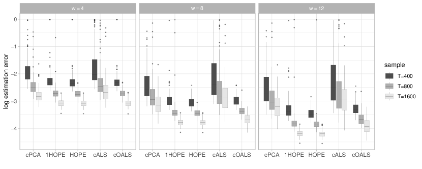
Figure 9: Boxplots of the logarithm of the estimation error under experiment configuration IV. Five methods with three choices of sample size $T$ are considered in total. Three columns correspond to three signal strength $w=4,8,12$.

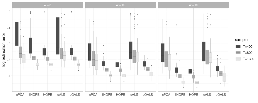
Figure 10: Boxplots of the logarithm of the estimation error under experiment configuration V. Five methods with three choices of sample size $T$ are considered in total. Three columns correspond to three signal strength $w=5,10,15$.

References

- Ahn and Horenstein, (2013) Ahn, S. C. and Horenstein, A. R. (2013). Eigenvalue ratio test for the number of factors. Econometrica, 81(3):1203–1227.
- Alter and Golub, (2005) Alter, O. and Golub, G. H. (2005). Reconstructing the pathways of a cellular system from genome-scale signals by using matrix and tensor computations. Proceedings of the National Academy of Sciences, 102(49):17559–17564.
- (3) Anandkumar, A., Ge, R., Hsu, D., and Kakade, S. M. (2014a). A tensor approach to learning mixed membership community models. Journal of Machine Learning Research, 15(1):2239–2312.
- (4) Anandkumar, A., Ge, R., Hsu, D., Kakade, S. M., and Telgarsky, M. (2014b). Tensor decompositions for learning latent variable models. Journal of Machine Learning Research, 15:2773–2832.
- (5) Anandkumar, A., Ge, R., and Janzamin, M. (2014c). Guaranteed non-orthogonal tensor decomposition via alternating rank-1 updates. arXiv preprint arXiv:1402.5180.
- Auddy and Yuan, (2020) Auddy, A. and Yuan, M. (2020). Perturbation bounds for orthogonally decomposable tensors and their applications in high dimensional data analysis. arXiv preprint arXiv:2007.09024.
- Auffinger et al., (2013) Auffinger, A., Arous, G. B., and Černỳ, J. (2013). Random matrices and complexity of spin glasses. Communications on Pure and Applied Mathematics, 66(2):165–201.
- Bai, (2003) Bai, J. (2003). Inferential theory for factor models of large dimensions. Econometrica, 71(1):135–171.
- Bai and Ng, (2002) Bai, J. and Ng, S. (2002). Determining the number of factors in approximate factor models. Econometrica, 70(1):191–221.
- Bai and Ng, (2007) Bai, J. and Ng, S. (2007). Determining the number of primitive shocks in factor models. Journal of Business & Economic Statistics, 25(1):52–60.
- Bai and Wang, (2014) Bai, J. and Wang, P. (2014). Identification theory for high dimensional static and dynamic factor models. Journal of Econometrics, 178(2):794–804.
- Bai and Wang, (2015) Bai, J. and Wang, P. (2015). Identification and bayesian estimation of dynamic factor models. Journal of Business & Economic Statistics, 33(2):221–240.
- Bekker, (1986) Bekker, P. (1986). A note on the identification of restricted factor loading matrices. Psychometrika, 51:607–611.
- Bi et al., (2018) Bi, X., Qu, A., and Shen, X. (2018). Multilayer tensor factorization with applications to recommender systems. Annals of Statistics, 46(6B):3308–3333.
- Bradley, (2005) Bradley, R. C. (2005). Basic properties of strong mixing conditions. a survey and some open questions. Probability Surveys, 2:107–144.
- Chamberlain and Rothschild, (1983) Chamberlain, G. and Rothschild, M. (1983). Arbitrage, factor structure, and mean-variance analysis on large asset markets. Econometrica, 51(5):1281–1304.
- (17) Chen, E. Y., Fan, J., and Li, E. (2020a). Statistical inference for high-dimensional matrix-variate factor model. arXiv preprint arXiv:2001.01890.
- Chen et al., (2019) Chen, E. Y., Tsay, R. S., and Chen, R. (2019). Constrained factor models for high-dimensional matrix-variate time series. Journal of the American Statistical Association, pages 1–37.
- (19) Chen, E. Y., Xia, D., Cai, C., and Fan, J. (2020b). Semiparametric tensor factor analysis by iteratively projected svd. arXiv preprint arXiv:2007.02404.
- Chen et al., (2021) Chen, R., Yang, D., and Zhang, C.-H. (2021). Factor models for high-dimensional tensor time series. Journal of the American Statistical Association, (just-accepted):1–59.
- Comon et al., (2009) Comon, P., Luciani, X., and De Almeida, A. L. (2009). Tensor decompositions, alternating least squares and other tales. Journal of Chemometrics: A Journal of the Chemometrics Society, 23(7-8):393–405.
- De Lathauwer et al., (2000) De Lathauwer, L., De Moor, B., and Vandewalle, J. (2000). On the best rank-1 and rank-(, ,…, ) approximation of higher-order tensors. SIAM Journal on Matrix Analysis and Applications, 21(4):1324–1342.
- Fan et al., (2011) Fan, J., Liao, Y., and Mincheva, M. (2011). High dimensional covariance matrix estimation in approximate factor models. Annals of Statistics, 39(6):3320.
- Fan et al., (2013) Fan, J., Liao, Y., and Mincheva, M. (2013). Large covariance estimation by thresholding principal orthogonal complements. Journal of the Royal Statistical Society: Series B (Statistical Methodology), 75(4):603–680.
- Fan et al., (2016) Fan, J., Liao, Y., and Wang, W. (2016). Projected principal component analysis in factor models. Annals of Statistics, 44(1):219–254.
- Fan and Yao, (2003) Fan, J. and Yao, Q. (2003). Nonlinear Time Series: Nonparametric and Parametric Methods. Springer Series in Statistics. Springer-Verlag, New York.
- Forni et al., (2000) Forni, M., Hallin, M., Lippi, M., and Reichlin, L. (2000). The generalized dynamic-factor model: Identification and estimation. The Review of Economics and Statistics, 82(4):540–554.
- Forni et al., (2004) Forni, M., Hallin, M., Lippi, M., and Reichlin, L. (2004). The generalized dynamic factor model consistency and rates. Journal of Econometrics, 119(2):231–255.
- Forni et al., (2005) Forni, M., Hallin, M., Lippi, M., and Reichlin, L. (2005). The generalized dynamic factor model: one-sided estimation and forecasting. Journal of the American Statistical Association, 100(471):830–840.
- Fosdick and Hoff, (2014) Fosdick, B. K. and Hoff, P. D. (2014). Separable factor analysis with applications to mortality data. Annals of Applied Statistics, 8(1):120.
- Hallin and Liška, (2007) Hallin, M. and Liška, R. (2007). Determining the number of factors in the general dynamic factor model. Journal of the American Statistical Association, 102(478):603–617.
- (32) Han, Y., Chen, R., Yang, D., and Zhang, C.-H. (2020a). Tensor factor model estimation by iterative projection. arXiv preprint arXiv:2006.02611.
- (33) Han, Y., Zhang, C.-H., and Chen, R. (2020b). Rank determination in tensor factor model. arXiv preprint arxiv:2011.07131.
- Hao et al., (2020) Hao, B., Zhang, A., and Cheng, G. (2020). Sparse and low-rank tensor estimation via cubic sketchings. IEEE Transactions on Information Theory.
- Håstad, (1990) Håstad, J. (1990). Tensor rank is NP-complete. Journal of Algorithms, 11(4):644–654.
- Hillar and Lim, (2013) Hillar, C. J. and Lim, L.-H. (2013). Most tensor problems are np-hard. Journal of the ACM (JACM), 60(6):1–39.
- Hoff, (2011) Hoff, P. D. (2011). Separable covariance arrays via the tucker product, with applications to multivariate relational data. Bayesian Analysis, 6(2):179–196.
- Hoff, (2015) Hoff, P. D. (2015). Multilinear tensor regression for longitudinal relational data. Annals of Applied Statistics, 9(3):1169.
- Kolda and Bader, (2009) Kolda, T. G. and Bader, B. W. (2009). Tensor decompositions and applications. SIAM Review, 51(3):455–500.
- Kuleshov et al., (2015) Kuleshov, V., Chaganty, A., and Liang, P. (2015). Tensor factorization via matrix factorization. In Artificial Intelligence and Statistics, pages 507–516. PMLR.
- Lam and Yao, (2012) Lam, C. and Yao, Q. (2012). Factor modeling for high-dimensional time series: inference for the number of factors. Annals of Statistics, 40(2):694–726.
- Lam et al., (2011) Lam, C., Yao, Q., and Bathia, N. (2011). Estimation of latent factors for high-dimensional time series. Biometrika, 98(4):901–918.
- Liu et al., (2012) Liu, J., Musialski, P., Wonka, P., and Ye, J. (2012). Tensor completion for estimating missing values in visual data. IEEE Transactions on Pattern Analysis and Machine Intelligence, 35(1):208–220.
- Liu et al., (2014) Liu, Y., Shang, F., Fan, W., Cheng, J., and Cheng, H. (2014). Generalized higher-order orthogonal iteration for tensor decomposition and completion. In Advances in Neural Information Processing Systems, pages 1763–1771.
- Merlevède et al., (2011) Merlevède, F., Peligrad, M., and Rio, E. (2011). A bernstein type inequality and moderate deviations for weakly dependent sequences. Probability Theory and Related Fields, 151(3-4):435–474.
- Neudecker, (1990) Neudecker, H. (1990). On the identification of restricted factor loading matrices: An alternative condition. Journal of Mathematical Psychology, 34(2):237–241.
- Omberg et al., (2007) Omberg, L., Golub, G. H., and Alter, O. (2007). A tensor higher-order singular value decomposition for integrative analysis of dna microarray data from different studies. Proceedings of the National Academy of Sciences, 104(47):18371–18376.
- Pan and Yao, (2008) Pan, J. and Yao, Q. (2008). Modelling multiple time series via common factors. Biometrika, 95(2):365–379.
- Pena and Box, (1987) Pena, D. and Box, G. E. (1987). Identifying a simplifying structure in time series. Journal of the American statistical Association, 82(399):836–843.
- Richard and Montanari, (2014) Richard, E. and Montanari, A. (2014). A statistical model for tensor PCA. In Advances in Neural Information Processing Systems, volume 27.
- Rosenblatt, (2012) Rosenblatt, M. (2012). Markov Processes, Structure and Asymptotic Behavior: Structure and Asymptotic Behavior, volume 184. Springer Science & Business Media.
- Sharan and Valiant, (2017) Sharan, V. and Valiant, G. (2017). Orthogonalized ALS: A theoretically principled tensor decomposition algorithm for practical use. In International Conference on Machine Learning, pages 3095–3104. PMLR.
- Stock and Watson, (2002) Stock, J. H. and Watson, M. W. (2002). Forecasting using principal components from a large number of predictors. Journal of the American Statistical Association, 97(460):1167–1179.
- Sun and Li, (2017) Sun, W. W. and Li, L. (2017). Store: sparse tensor response regression and neuroimaging analysis. Journal of Machine Learning Research, 18(1):4908–4944.
- Sun et al., (2017) Sun, W. W., Lu, J., Liu, H., and Cheng, G. (2017). Provable sparse tensor decomposition. Journal of the Royal Statistical Society: Series B (Statistical Methodology), 3(79):899–916.
- Tong, (1990) Tong, H. (1990). Non-linear Time Series: a Dynamical System Approach. Oxford University Press.
- Tsay, (2005) Tsay, R. S. (2005). Analysis of Financial Time Series, volume 543. John Wiley & Sons.
- Tsay and Chen, (2018) Tsay, R. S. and Chen, R. (2018). Nonlinear Time Series Analysis, volume 891. John Wiley & Sons.
- Wang et al., (2019) Wang, D., Liu, X., and Chen, R. (2019). Factor models for matrix-valued high-dimensional time series. Journal of Econometrics, 208(1):231–248.
- Wang and Li, (2020) Wang, M. and Li, L. (2020). Learning from binary multiway data: Probabilistic tensor decomposition and its statistical optimality. Journal of Machine Learning Research, 21(154):1–38.
- Wang and Song, (2017) Wang, M. and Song, Y. (2017). Tensor decompositions via two-mode higher-order SVD (HOSVD). In Artificial Intelligence and Statistics, pages 614–622. PMLR.
- Wang and Lu, (2017) Wang, P.-A. and Lu, C.-J. (2017). Tensor decomposition via simultaneous power iteration. In International Conference on Machine Learning, pages 3665–3673. PMLR.
- Wedin, (1972) Wedin, P.-Å. (1972). Perturbation bounds in connection with singular value decomposition. BIT Numerical Mathematics, 12(1):99–111.
- Zhang and Xia, (2018) Zhang, A. and Xia, D. (2018). Tensor SVD: Statistical and computational limits. IEEE Transactions on Information Theory, 64(11):7311–7338.
- Zhou et al., (2013) Zhou, H., Li, L., and Zhu, H. (2013). Tensor regression with applications in neuroimaging data analysis. Journal of the American Statistical Association, 108(502):540–552.