Metric Assisted Stochastic Sampling (MASS) search for gravitational waves from binary black hole mergers

Abstract

We present a novel gravitational wave detection algorithm that conducts a matched filter search stochastically across the compact binary parameter space rather than relying on a fixed bank of template waveforms. This technique is competitive with standard template-bank-driven pipelines in both computational cost and sensitivity. However, the complexity of the analysis is simpler allowing for easy configuration and horizontal scaling across heterogeneous grids of computers. To demonstrate the method we analyze approximately one month of public LIGO data from July 27 00:00 2017 UTC – Aug 25 22:00 2017 UTC and recover eight known confident gravitational wave candidates. We also inject simulated binary black hole (BBH) signals to demonstrate the sensitivity.

I Introduction

Advanced LIGO directly detected gravitational waves (GWs) for the first time in 2015 from the merger of two black holes each about 30 times the mass of our Sun Abbott et al. (2016a). The second confident binary black hole (BBH) observation came just three months later Abbott et al. (2016b). Since then, the LIGO and Virgo Collaborations have detected a total of 90 compact binary mergers Abbott et al. (2019, 2020a, 2021a); Collaboration et al. (2021), including two neutron star mergers Abbott et al. (2017, 2020b) and two neutron star-black hole mergers Abbott et al. (2021b). LIGO and Virgo have made their data public Trovato (2020) resulting in several new BBH discoveries by the community Zackay et al. (2019a); Venumadhav et al. (2019a); Zackay et al. (2019b); Venumadhav et al. (2019b); Nitz et al. (2021); Abbott et al. (2021c).

Historically, gravitational wave searches for compact binary coalescence have relied on matched filtering Finn and Chernoff (1993); Owen (1996); Owen and Sathyaprakash (1999), with several groups building on matched filtering as the foundation for their algorithms Allen et al. (2012); Cannon et al. (2012); Babak et al. (2013); Nitz et al. (2017); Adams et al. (2016); Venumadhav et al. (2019b). These techniques rely on fixed banks of templates Owen (1996); Harry et al. (2009); Ajith et al. (2014) and are known to scale poorly to high dimensional spaces Harry et al. (2016). Stochastic sampling methods were first proposed to address gravitational wave detection in future searches for gravitational waves with LISA Cornish and Crowder (2005), but have not been widely used for detection in LIGO and Virgo data. Stochastic sampling techniques are, however, state-of-the art for the estimation of compact binary parameters once detections have been made Veitch et al. (2015); Ashton et al. (2019).

In this work we blend aspects of traditional matched filter searches, bank placement techniques, and stochastic sampling to create a new bank-less matched filter search for gravitational waves. While it remains to be seen what the broad applications of these techniques could be, we demonstrate a useful case study here by analyzing LIGO data from the Hanford and Livingston detectors from August 2017 et al. (LIGO Scientific Collaboration and Collaboration) to search for binary black hole mergers. We recover eight known gravitational wave candidates.

II Motivation

Our goal is to develop an offline compact binary search pipeline which is designed to detect gravitational waves in archival, LIGO, Virgo, and KAGRA data based on the GstLAL framework Messick et al. (2017); Sachdev et al. (2019); Cannon et al. (2021); gst . We distinguish that an offline analysis has less strict time-to-solution requirements (hours or days) compared to low-latency analysis where the time-to-solution needs to be seconds. We will not strive to reach the time-to-solution needs of low-latency analysis with the algorithm we present here. Our motivation for revisiting offline matched filter detection for gravitational waves is to more easily parallelize and deploy analysis across heterogeneous resources such as multiple concurrent sites on the LIGO and Virgo data grids, the Open Science Grid, campus resources, and commercial clouds. We aim to achieve this by having a simpler workflow than competing pipelines such as GstLAL. We also wish to simplify the setup required to conduct an analysis and to improve usability for new researchers wanting to learn about gravitational wave detection at scale. The intersection of these desires led us to consider new algorithmic approaches to searching the compact binary parameter space.

The Open Science Grid defines criteria for opportunistic computing as an application that “does not require message passing…has a small runtime between 1 and 24 hours…can handle being unexpectedly killed and restarted…” and “…requires running a very large number of small jobs rather than a few large jobs.” osg (2021). Our proposed workflow consists of parallel jobs that each search a small amount of gravitational-wave data from LIGO, Virgo and KAGRA without any interdependency between jobs. To contrast, the current GstLAL analysis workflow consists of a directed acyclic graph with more than ten levels of interdependent jobs. In this new approach, we target a $\sim$1–12 hour runtime for each job, the use of one CPU core per job, and $\sim 2$ GB of RAM required per job in order to maximize throughput on opportunistic compute resources. Each job implements a flexible checkpointing procedure allowing work to be periodically saved.

III Methods

In this work, we will conduct a matched-filter search for binary black holes with the goal of identifying the maximum likelihood parameters for candidate events over 4s coalescence-time windows using an analysis that foregoes the use of a pre-computed template bank and instead employs stochastic sampling of the binary parameter space. Our workflow consists of two stages. The first stage executes N parallel jobs that conduct the bulk of the cpu-intensive work - in this study, this first stage consisted of 2974 such jobs. The results of these parallel jobs are returned to a single location at which point a second stage is run to combine results, assess candidate significance, estimate the search sensivity and visualize the results. This second stage requires significantly lower computing power than the first stage, but is I/O intensive and is designed to be run potentially on local resources after grid jobs have completed.

In stage one, we begin by reading in gravitational wave data from each observatory. Next, we measure the data noise power spectrum and whiten the data using the inferred spectrum. We then stochastically sample the data by proposing jumps governed by a parameter space metric as described in Section III-D. For each jump, we generate the appropriate template waveform and then compute the matched filter signal-to-noise ratio (SNR) over a 6s stretch of time using 122s of data per calculation.

Within a 4s time window, we identify peaks in the matched filter output, known as triggers, for each detector that is being analyzed. For each collection of triggers, we perform signal consistency checks Messick et al. (2017), and calculate a likelihood ratio ranking statistic Cannon et al. (2015). If the new sample has a larger SNR than the previous sample, it is stored - otherwise a new jump is proposed.

A local estimate of the noise background is obtained by forming synthetic events from disjoint windows. This causes the time and phase difference between detectors of a single background event to be uniformly distributed, which is what we expect from noise events. This is a somewhat hybrid approach between the time-slide method Babak et al. (2013) and sampling methods Cannon et al. (2013) already employed in GW searches. The second stage gathers the candidate events, results of the simulated GW search, and the background samples to produce a final summary view of the analysis results. In order to estimate the sensitivity of our methods to detecting gravitational waves, we conduct a parallel analysis over the same data with simulated signals added and repeat the same process as described above.

The remainder of this section describes key elements of our methods in more detail.

III.1 Data

We assume a linear model for the gravitational wave strain data Finn and Chernoff (1993), $\mathbf{s}$, which is a vector of discretely sampled time points for a gravitational wave detector, $j$,

$$\mathbf{s}_{j}=\mathbf{h}(\vec{\theta}_{j})+\mathbf{n}_{j},$$ (1)

where: $\mathbf{h}(\vec{\theta}_{j})$ is an unknown gravitational waveform accurately modeled as a function of $\vec{\theta}_{j}=\{m_{1},m_{2},a_{1z},a_{2z},t_{j},\phi_{j},A_{j}\}$ with $m_{1},m_{2}$ being the component masses, $a_{1z},a_{2z}$ being the orbital-angular-momentum-aligned component spins and $t_{j},\phi_{j},A_{j}$ being the time of coalescence, phase of coalescence, and amplitude, all of which depend on exactly where the binary is with respect to the $j$th gravitational wave detector. $\mathbf{n}_{j}$ is a realization of detector noise. As a concrete example, in this work each job analyzes 800s stretches of data, divided into 4s windows sampled at 2048 Hz. Thus, after including the Fourier transform block length (124s), the dimension of each vector in the work described in this manuscript is 262144 sample points. In addition, each job also contains start padding (128s), and stop padding (32s). The templates have at least 6s of zero padding, which makes their length no more than 122s.

We assume that the noise samples are entirely uncorrelated between the gravitational wave observatories, but that the signals are correlated between observatories. In fact, we make the simplifying assumption that the gravitational waveform is identical between detectors except for an overall amplitude, $A_{j}$, time shift, $\Delta t_{j}$, and phase shift, $\Delta\phi_{j}$,  Allen et al. (2012),

$$\mathbf{h}(\vec{\theta}_{j}) =\Re\left(\mathcal{F}^{-1}\left[A_{j}e^{2\pi if\Delta t_{j}+\Delta\phi_{j}}\mathcal{F}\left[\mathbf{h}(\vec{\lambda},t,\phi)\right]\right]\right),$$ (2)

where $\mathcal{F}\left[\dots\right]$ denotes the unitary Fourier transform, and $\vec{\lambda}{}=\{m_{1},m_{2},a_{1z},a_{2z}\}$.

The exact realization of noise, $\mathbf{n}$, is not possible to predict, but we will assume it is well characterized as a multivariate normal distribution with a diagonal covariance matrix in the frequency domain, i.e., that it is stationary. However later on, particularly in Sec. III.4.6, we account for the fact that the data is often not stationary.

III.2 Spectrum estimation and whitening

We rely on the same spectrum estimation methods as described in Messick et al. (2017). Namely we use a median-mean, stream-based spectrum estimation technique that adjusts to changes in the noise spectrum on $\mathcal{O(\textrm{min})}$ time scales. The data are divided into 8s blocks with 6s overlap and the spectrum, $\mathbf{S}_{n}$ is estimated by windowing the input blocks with 2s of zero-padding on each side of the window. Since we analyze only 800s of data per job, we use a fixed spectrum over the job duration.

From here forward, we will work in a whitened basis for the data, namely that

$$\mathbf{s}_{j} \to\mathcal{F}\left[\mathbf{s}\right]\circ\left(\mathbf{S}_{n}\right)^{-1/2},$$ (3)

which implies that all components of $\mathbf{s}$ are transformed by the inverse noise amplitude spectrum. Therefore, if the amplitude of $\mathbf{h}$ is zero, $\mathbf{s}$ has components that satisfy $p(s_{i})=\left(2\pi\right)^{-1/2}\,e^{-s_{i}^{2}/2}$ with $\langle s_{i},s_{j}\rangle=\delta_{ij}$. In this whitened data basis, an inner product between two vectors is the dot product $\mathbf{u}\cdot\mathbf{v}$, and unit vectors are denoted as $\hat{\mathbf{u}}$. We adopt a normalization such that $\mathbf{h}\cdot\mathbf{h}=1$ and $\langle\mathbf{n}\cdot\mathbf{n}\rangle=\dim{\mathbf{n}}$. With these choices the SNR is given by $\rho(\vec{\theta}_{j})=\mathbf{h}(\vec{\theta}_{j})\cdot\mathbf{s}_{j}$. We can evaluate the SNR for the unknown phase and time of coalescence by defining a complex SNR

$$\rho(\vec{\lambda},t_{j},\phi_{j}) =\mathcal{F}^{-1}\left[\mathbf{h}(\vec{\lambda})\cdot\mathbf{s}_{j}\right]$$

$$+i\mathcal{F}^{-1}\left[\mathbf{h}(\vec{\lambda},\pi/2)\cdot\mathbf{s}_{j}\right],$$ (4)

which is a valid matched-filter output for a duration of time equal to the length of the data minus the length of the template. With at least 6s of zero-padding, the template length is 122s, and with each window using 128s of data, the matched-filter output is valid for a duration of 6s.

III.3 Simulation capabilities

We use the GstLAL data source module gst , which provides an interface into the LAL Simulation package lal . By providing a LIGO-LW XML format document containing simulation parameters, we can inject simulated strain into each of the currently operating ground-based gravitational wave detectors, LIGO, Virgo, KAGRA and GEO-600. When operating the pipeline in a simulation mode, gravitational wave events are reconstructed around a $\pm 2$s interval around the GPS second of the geocentric arrival time of the gravitational wave peak strain.

III.4 Parameter space sampling

The gravitational wave parameter space is explored stochastically, with Gaussian jump proposals and refinement steps that gradually reduce the jump size as the peak in SNR is identified. We will refer to this procedure as “sampling”. Our proposal distribution has a covariance matrix that depends on the location in the parameter space and the refinement level. It relies on computing the parameter space metric, $\mathbf{g}$ Owen (1996), which is described more in the next section. We define a sequence of two parameters that control how the sampling is done, namely $\sigma_{k}$, which controls the jump size and $N_{k}$ which controls the number of samples to reject at each level, $k$, before moving on to the next. How exactly to define these parameters is certainly a topic for future research. Our choices here were determined empirically for the particular search we have done. We define,

$$\sigma_{k} =10^{1-k},$$ (5)

$$N_{k} =\begin{cases}500&(k=0)\\ 100&(k>0)\end{cases},$$ (6)

for $k=0\dots n$ where $k$ is terminated based on the mismatch as in step 7 below. We define the characteristic jump proposal distance as,

$$\delta_{k}(\vec{\lambda}):=\sigma_{k}|\mathbf{g}(\vec{\lambda})|^{1/8},$$ (7)

where $\vec{\lambda}$ is the set of intrinsic parameters as defined before, and $\delta^{2}_{k}$ is the template mismatch.

Gravitational waves are searched over 4 s windows of coalescence time using the following procedure.

1. Establish a bounding box in the physical parameter space to search over

2. Pick a starting parameter point somewhere in the middle of the parameter space. We use the approximate expression for template count in Owen (1996) to estimate a good central point.

3. Evaluate the SNR at this point and set a counter to zero.

4. Sample from a sampling function $\Theta(\delta_{k},\vec{\lambda})$, which is described in detail below in Sec. III.4.4.

5. Check that the new point lies within boundaries established in step 1 and apply any constraint functions. If the point fails to fall within the constraints, go to step 4.

6. Evaluate the SNR at the new point. If the point has a higher SNR than the previous sample, update the sample and reset the counter to zero. If the point has a lower SNR, increment the counter.

7. If the counter is less than $N_{k}$, go back to step 4. If the counter is greater than or equal to $N_{k}$, check $\delta^{2}$, where $\delta^{2}$ is the template mismatch between the current and previous sample point. If $\delta^{2}<0.1$, terminate the sampling. Otherwise, increment $k$, reset the counter, and proceed to step 4.

III.4.1 Computation of the binary parameter space metric

We define the match between adjacent compact binary waveforms in the space of intrinsic parameters as:

$$m(\vec{\lambda},\vec{\lambda}+\vec{\Delta\lambda}) =\max_{\phi_{c},t_{c},A}\left[\,\hat{\mathbf{h}}(\vec{\lambda})\,\cdot\,\hat{\mathbf{h}}(\vec{\lambda}+\vec{\Delta\lambda})\,\right].$$ (8)

where the maximum is over extrinsic parameters $\{t_{c},\phi_{c},A\}$. Note that $m(\vec{\lambda},\vec{\lambda})=1$. We also introduce a shorthand for computing the match along a deviation in only one coordinate as:

$$m(\vec{\lambda},\vec{\lambda}+\vec{\Delta\lambda}_{i}) =\max_{\phi_{c},t_{c},A}\left[\,\hat{\mathbf{h}}(\vec{\lambda})\,\cdot\,\hat{\mathbf{h}}(\vec{\lambda}+\vec{\Delta\lambda}_{i})\,\right],$$ (9)

where it is assumed that $\Delta\vec{\lambda}_{i}$ is nonzero only along a given coordinate direction.

It has previously been shown Owen (1996) that is possible to derive a metric on the space of intrinsic parameters describing compact binary waveforms by expanding our definition of the match locally e.g. about $\Delta\lambda=0$ as follows,

$$m(\vec{\lambda},\vec{\lambda}+\vec{\Delta\lambda})\approx 1+$$

$$\frac{1}{2}\frac{\partial^{2}}{\partial\Delta\lambda_{i}\partial\Delta\lambda_{j}}m(\vec{\lambda},\vec{\lambda}+\vec{\Delta\lambda})\big{|}_{\vec{\Delta\lambda}=0}\Delta\lambda_{i}\Delta\lambda_{j}$$ (10)

which suggests the metric

$$g_{ij}(\vec{\lambda})=-\frac{1}{2}\frac{\partial^{2}}{\partial\Delta\lambda_{i}\partial\Delta\lambda_{j}}m(\vec{\lambda},\vec{\lambda}+\vec{\Delta\lambda})\big{|}_{\vec{\Delta\lambda}=0},$$ (11)

The mismatch between templates, $\delta^{2}=1-m$ becomes

$$\delta(\vec{\lambda},\vec{\Delta\lambda})^{2} \approx\vec{\Delta\lambda}^{T}\,\mathbf{g}(\vec{\lambda})\,\vec{\Delta\lambda},$$ (12)

In this work, the components of the metric are evaluated with second-order finite differencing,

$$g_{ii}(\vec{\lambda}) =-\frac{1}{2}\left[\frac{m(\vec{\lambda},\vec{\lambda}+\Delta\vec{\lambda}_{i})+m(\vec{\lambda},\vec{\lambda}-\Delta\vec{\lambda}_{i})-2}{|\Delta\vec{\lambda}_{i}|^{2}}\right],$$ (13)

and

$$g_{ij}(\vec{\lambda}) =-\frac{1}{2}\frac{1}{4|\Delta\vec{\lambda}_{i}||\Delta\vec{\lambda}_{j}|}\times$$

$$\biggr{[}\hskip 6.0ptm(\vec{\lambda},\vec{\lambda}+\Delta\vec{\lambda}_{i}+\Delta\vec{\lambda}_{j})$$

$$\hskip 10.0pt-m(\vec{\lambda},\vec{\lambda}+\Delta\vec{\lambda}_{i}-\Delta\vec{\lambda}_{j})$$

$$\hskip 10.0pt-m(\vec{\lambda},\vec{\lambda}-\Delta\vec{\lambda}_{i}+\Delta\vec{\lambda}_{j})$$

$$\hskip 10.0pt+m(\vec{\lambda},\vec{\lambda}-\Delta\vec{\lambda}_{i}-\Delta\vec{\lambda}_{j})\hskip 6.0pt\biggr{]},$$ (14)

for the off diagonal terms. However, we use a more efficient formula for the off diagonal terms, in which the number of template evaluations is the same, but the number of match calculations is reduced:

$$g_{ij}(\vec{\lambda}) =-\frac{1}{2}\frac{1}{2|\Delta\vec{\lambda}_{i}||\Delta\vec{\lambda}_{j}|}\times$$

$$\biggr{[}\hskip 6.0ptm(\vec{\lambda},\vec{\lambda}+\Delta\vec{\lambda}_{i}+\Delta\vec{\lambda}_{j})-m(\vec{\lambda},\vec{\lambda}+\Delta\vec{\lambda}_{i})$$

$$\hskip 10.0pt-m(\vec{\lambda},\vec{\lambda}+\Delta\vec{\lambda}_{j})+2-m(\vec{\lambda},\vec{\lambda}-\Delta\vec{\lambda}_{i})$$

$$\hskip 10.0pt-m(\vec{\lambda},\vec{\lambda}-\Delta\vec{\lambda}_{j})+m(\vec{\lambda},\vec{\lambda}-\Delta\vec{\lambda}_{i}-\Delta\vec{\lambda}_{j})\hskip 6.0pt\biggr{]}$$ (15)

The sampling method described in section 4 below will not make jumps in coalescence time, therefore the time component is projected out  Owen (1996),

$$g_{ij}(\vec{\lambda}) \to g_{ij}(\vec{\lambda})-\frac{g_{ti}(\vec{\lambda})\,g_{tj}(\vec{\lambda})}{g_{tt}(\vec{\lambda})}.$$ (16)

III.4.2 Choice of coordinates

We sought out a coordinate system that maps the masses and spins to be in the interval $\left[-\infty,\infty\right]$. We also want to choose well measured physical parameters for mass and spin in at least one dimension each. Therefore, we use the following coordinates to evaluate the metric

$$\lambda_{1} =\log_{10}\left[\frac{(m_{1}m_{2})^{3/5}}{(m_{1}+m_{2})^{1/5}}\right]$$ (17)

$$\lambda_{2} =\log_{10}(m_{2})$$ (18)

$$\lambda_{3} =\tan\left[\left(\frac{\pi}{2}\right)\left(\frac{a_{1z}m_{1}+a_{2z}m_{2}}{m_{1}+m_{2}}\right)\right]$$ (19)

$$\lambda_{4} =\tan\left[\left(\frac{\pi}{2}\right)\left(\frac{a_{1z}m_{1}-a_{2z}m_{2}}{m_{1}+m_{2}}\right)\right]$$ (20)

III.4.3 Pathologies of the numerical metric

For certain regions of the parameter space the metric is nearly singular which leads to numerical errors causing a non positive definite matrix. To fix this, we conduct an eigenvalue decomposition of $g_{ij}$

$$g_{ij} =q_{ik}\,\beta^{k}\,q^{-1}_{kj}$$ (21)

We then define a new set of eigenvalues

$$\beta_{\mathrm{min}} \equiv\max_{k}\left[\beta^{k}\right]\times\epsilon$$ (22)

$$(\beta^{k})^{\prime} =\begin{cases}\beta_{\mathrm{min}},&\beta^{k}<\beta_{min}\\ \beta^{k},&\text{otherwise},\end{cases}$$ (23)

where $\epsilon$ is a parameter which we will call the aspect ratio. We define the new metric as

$$g_{ij} \to q_{ik}\,(\beta^{k})^{\prime}\,q^{-1}_{kj}$$ (24)

In practice we find that sampling is better when we artificially distort the metric by setting $\epsilon=.1$ for the broadest refinement level, and $\epsilon=.0001$ for all other levels, and we have done so in this work, though this should be a direction of future work.

III.4.4 Drawing random samples from $\Theta(\delta_{k},\vec{\lambda})$

When sampling, we desire to have a jump proposal distribution that effectively probes the space by not making jumps that are either too near or too far. The calculation of the parameter space metric $\mathbf{g}$ enables that. We wish to propose a jump from $\vec{\theta}\to\vec{\theta}+\Delta\vec{\theta}$ such that the expected mismatch is $\delta^{2}$. The metric described in previous sections only applies to the intrinsic parameters. For the extrinsic parameters, our jump proposal will always choose those values of $t$ and $\phi$ which maximize the SNR. At every accepted jump point, the metric is calculated locally, which requires 21 template evaluations, including the diagonal and off diagonal terms, as specified in Sec. III.4.1. However, we can afford to calculate coarse versions of the template waveform, since the match we need to calculate is between two adjacent templates. This means the waveform calculation cost is not high. The distance between adjacent templates to calculate the match at, $\Delta\vec{\lambda}_{i}$ as defined in Sec. III.4.1 is hardcoded, and is the same for all iterations of the sampling procedure.

To facilitate jumping in the intrinsic parameters, we make a coordinate basis transformation in which the new basis has a Euclidian metric. The transformation matrix $\mathbf{M}$ will then be used to transform the coordinates

$$\vec{\lambda}^{\prime} =\mathbf{M}\vec{\lambda}.$$ (25)

To solve for $\mathbf{M}$ we rely on the fact that distance is invariant giving

$$\delta^{2} =\vec{\Delta\lambda}^{T}\,\mathbf{g}\,\vec{\Delta\lambda}$$ (26)

$$=(\vec{\Delta\lambda}^{\prime})^{T}\,\mathbf{g}^{\prime}\,\vec{\Delta\lambda}^{\prime}$$ (27)

$$=(\vec{\Delta\lambda}^{\prime})^{T}\,\mathbf{M}^{T}\mathbf{g}\,\mathbf{M}\,\vec{\Delta\lambda}^{\prime}$$ (28)

Setting $\mathbf{g}^{\prime}=\mathbf{I}$ gives

$$\mathbf{I} =\mathbf{M}^{T}\mathbf{g}\,\mathbf{M}$$ (29)

$$\mathbf{M}^{-1}(\mathbf{M}^{T})^{-1} =\mathbf{g}$$ (30)

$$\mathbf{g}^{-1} =\mathbf{M}^{T}\mathbf{M}$$ (31)

The last line implies that we can solve for $\mathbf{M}$ by taking the Cholesky decomposition of the inverse metric tensor. Once obtaining $\mathbf{M}$ we can produce random samples with an expected mismatch by defining,

$$\Theta(\delta_{k},\vec{\lambda}) :=\delta_{k},\vec{\lambda}\to\vec{\lambda}+\delta_{k}\mathbf{M}^{T}\,\vec{\mathcal{N}},$$ (32)

where $\vec{\mathcal{N}}$ is a 4-dimensional vector with random components satisfying $p(\mathcal{N}_{i})=\sqrt{1/2\pi}\exp\left[-\mathcal{N}_{i}^{2}/2\right]$

III.4.5 Parameter space constraints

The previously defined sampling function can produce samples that, while physical, may be outside of the desired search range. We implement a series of user-defined constraints that will reject samples drawn from $\Theta(\delta_{k},\vec{\lambda})$. These are:

$\mathbf{m_{1},m_{2},a_{1},a_{2}}$

The user can specify a bounding-box in component masses and $z$-component spins. Samples outside this bounding box are rejected.

$\boldsymbol{\eta}$

The user can specify a minimum symmetric mass ratio, $\eta\equiv(m_{1}m_{2})/(m_{1}+m_{2})^{2}$, below which samples will be rejected.

$\mathcal{M}$

The user can specify a chirp mass range outside of which samples will be rejected.

III.4.6 Glitch Rejection

Glitches Ashton et al. (2021); Davis et al. (2020) are non-stationarity and non-Gaussian transient noise artefacts of instrumental or environmental origin found in the data. We employ a novel data-driven technique to reject short-duration glitches, using two parameters, the bandwidth, and the effective spin parameter $\chi$. The bandwidth is the standard deviation of frequency weighted by template amplitude. It is defined as Fairhurst (2009):

$$\text{bandwidth}^{2}=\frac{\int|\hat{\mathbf{h}}(\vec{\lambda})|^{2}f^{2}df/\mathbf{S}_{n}}{\int|\hat{\mathbf{h}}(\vec{\lambda})|^{2}df/\mathbf{S}_{n}}-\left(\frac{\int|\hat{\mathbf{h}}(\vec{\lambda})|^{2}fdf/\mathbf{S}_{n}}{\int|\hat{\mathbf{h}}(\vec{\lambda})|^{2}df/\mathbf{S}_{n}}\right)^{2}$$ (33)

whereas $\chi$ is defined as:

$$\chi=\frac{m_{1}a_{1z}+m_{2}a_{2z}}{m_{1}+m_{2}}$$ (34)

It has been found that short-duration glitches ring up templates which exclusively occupy the low bandwidth-low $\chi$ region in bandwidth-$\chi$ space, and that this region is not occupied by gravitational wave signals. This is illustrated in Fig. 1. As part of the simulation campaign we performed (Refer to Sec. IV.3 for details), we found that only 28 injections out of 112526 fell into the glitch region. Minimizing this number by fine-tuning the boundary of the glitch region would be a direction for future work. We define the glitch region as:

$$\text{bandwidth}\times(1+\chi)\leq 20$$ (35)

Any trigger which falls in this region is not considered as a gravitational wave candidate. Similarly, any time-slid background samples falling in the glitch region are eliminated, and not used for background estimation. Triggers are explained in more detail in the next subsection, whereas background estimation is explained in section E.

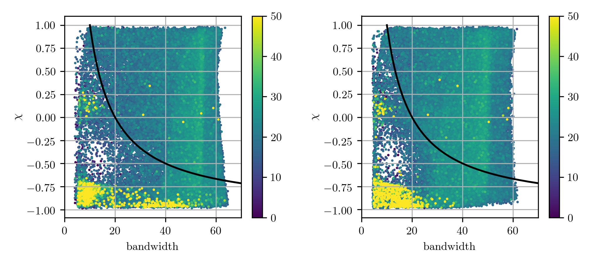
Figure 1: Triggers found in one month’s data for Hanford (left) and Livingston (right), colored by their log-likelihood ratio. All the bright points to the right of the boundary are known gravitational wave candidates, and all those to the left of the boundary are glitches, and so not considered gravitational wave candidates, and not used for background estimation.

III.4.7 Computing the log-likelihood ratio, $\mathcal{L}$

We generally follow the same procedure for ranking candidates as described in Cannon et al. (2013, 2015); Hanna et al. (2020) with a couple of notable exceptions. First, we only implement a subset of the terms used in the GstLAL-inspiral pipeline – it will be the subject of future work to include more. Second, we approximate some of the data driven noise terms with analytic functions. Third, we adopt a normalization so that for signals, the log likelihood ratio, $\mathcal{L}$ is approximately $\rho^{2}/2$, where $\rho$ is the network matched filter SNR defined as the squareroot of the sum of the squares of the SNRs found in each observatory. We use the following terms in the log likelihood ratio:

$\mathcal{L}(\vec{\rho},\vec{\xi^{2}})$

We approximate this term of the log likelihood ratio as

$$\mathcal{L}(\vec{\rho},\vec{\xi^{2}}) =\sum_{i}\mathcal{L}_{i}(\rho_{i},\xi^{2}_{i})$$ (36)

$$\text{with}\hskip 3.0pt\mathcal{L}_{i}(\rho_{i},\xi^{2}_{i}) =\rho_{i}^{2}e^{-4x_{i}^{2}}/2-4x_{i}^{2}$$ (37)

where $x_{i}\equiv\max\{0,\xi_{i}^{2}-1-0.0005\rho_{i}^{2}\}$ for each of the $i$ detectors which are assumed to be independent. The $-4x_{i}^{2}$ term acts as a penalty for high $\xi^{2}_{i}$ values, and helps eliminate glitches.

$\mathcal{L}(\Delta\vec{t},\Delta\vec{\phi},\Delta\vec{\rho})$

for this term we follow the procedure in Hanna et al. (2020) with two changes. We do not include the $\rho^{-4}$ term. We do this because we are not constructing a data driven noise term like GstLAL-inspiral, so it’s not necessary to have the corresponding signal term. We also normalize the result to be 0 when only one detector is operating. This is useful for achieving the normalization discussed above. These changes have the effect of making this term $\sim 0$ for things that are consistent with signals.

$\mathcal{L}(\vec{T})$

this term quantifies the probability of having “triggered” the combination of the gravitational wave detectors in which the event was found and is a function of the detectors’ sensitivity. We will describe triggering in more detail below. For example, it is unlikely that only the least sensitive detector would be triggered for a real gravitational wave event, so this term would be negative in that case. This term is complementary to the previous term but accounts for events lacking triggers.

$\mathcal{L}(\vec{D}_{H})$

this term quantifies the relative likelihood of detecting an event based on the detector horizon BNS distances, $(D_{H})_{i}$. We normalize to the horizon distance of LIGO Livingston during O3$\sim 315$ Mpc.

$$\mathcal{L}(\vec{D}_{H}) =\ln\left(\frac{\max_{i}\left[\{(D_{H})_{i}\}\right]}{315Mpc}\right)^{3}$$ (38)

The log-likelihood ratio, $\mathcal{L}$ is then given by

$$\mathcal{L} =\mathcal{L}(\vec{\rho},\vec{\xi^{2}})+\mathcal{L}(\Delta\vec{t},\Delta\vec{\phi},\Delta\vec{\rho})$$

$$+\mathcal{L}(\vec{T})+\mathcal{L}(\vec{D}_{H})$$ (39)

For each sample drawn in step 4, we construct a template waveform $\mathbf{h}(\vec{\lambda})$, and filter that waveform against the data in each detector stream producing an SNR time series over a 6s period, including 1s padding on either side. We then find the peak SNR in the middle 4s window in each detector and record the time, phase, SNR, and $\xi^{2}$ of each peak, which we call a “trigger”. For the collection of triggers, we cycle through every detector combination - for example, if analyzing {H,L,V}, we cycle through {HLV, HL, HV, LV, H, L, V} and evalute the likelihood ratio for each combination. We then keep the maximum $\mathcal{L}$ found over these detector combinations. This is done to mitigate the effect of bad data (noisy data and possibly also glitchy data) in one detector. Hence, triggers are obtained by maximizing SNR over 4s windows, whereas the detectors to be considered for the trigger are obtained by maximizing the likelihood ratio over all possible detector combinations. Note that the SNR maximization for updating the sample discussed in step 6 is a seperate procedure from either of these.

III.5 Background estimation

We treat windows recovered as single triggers and windows recovered as coincidences differently while estimating the background. For single trigger windows, the foreground sample itself is used as the background sample representing that window. To estimate the coincident background, we form false coincidences from a given job which analyzes 800s of data in 200 coalescence time windows. To form false coincidences, we shift the windows in time with respect to each other. We then draw samples randomly from all single detector triggers. For each recovered false coincidence, we compute a $\mathcal{L}$ and histogram the result. This process is then repeated 100 times with different time offsets to increase the amount of background we have. This background is given an appropriate weight so that the ratio of singles to coincidences in the background and foreground is the same, as well as to ensure that the background is normalized. Using the $\mathcal{L}$ histogram for the background, false alarm rates (FARs) are assigned to all the triggers. One point to note is that the windows in which we detect events are not used to form combinations so as to not contaminate the background with signals.

IV Results

IV.1 Data set

We analyze public gravitational wave data from LIGO taken from July 27 00:00 2017 UTC – Aug 25 22:00 2017 UTC during advanced LIGO’s second observing run. We choose segments of data with a minimum length of 1200s for each of the LIGO detectors. From those segments we form coincident segments. Jobs require 128s of start padding, 32s of end padding and 124s for the Fourier transform block to produce triggers. Thus, each job can analyze a minimum of 288s (which produces triggers for for a single 4s window) and we choose a maximum duration of 1084s to produce 800s of triggers over 200 windows. Jobs are overlapped so that triggers are produced contiguously.

After accounting for the segment selection effects, we analyzed approximately 20.17 days of coincident data.

IV.2 Search parameter space

We search for gravitational wave candidates with component masses between 0.9–400 M_⊙ with $z$-component spins between $-1$ and 1. We conduct the matched filter integration between 10–1024 Hz.

IV.3 Simulation set

In order to ascertain our sensitivity to gravitational wave signals of the type discovered in this data, we conducted a simulation campaign with 112526 simulated signals having a 32 M_⊙ mean component mass and standard deviation of 4.0 M_⊙ with aligned dimensionless spins up to 0.25 and a maximum redshift of 1 isotropically distributed in location. The injections were distributed uniformly in comoving volume. The red-shifted component mass distribution is visualized in Fig. 2. The injection set was specifically created for the BBH parameter space. We do not make any claims about the sensitivity of our pipeline in other lower mass parameter spaces.

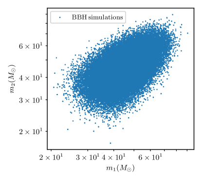
Figure 2: Distribution of component masses as measured at Earth for the BBH simulation set.

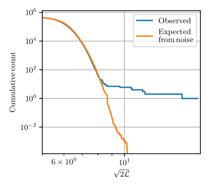
Figure 3: Cumulative histograms of our search results as a function of likelihood ratio. The orange line represents the corresponding histogram expected from noise during the same time frame.

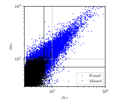
Figure 4: Distribution of injected SNRs for recovered injections above $\mathcal{L}=35(\sqrt{2\mathcal{L}}=8.37$). Missed injections with network SNR above 12 and detector SNRs greater than 7 (indicated by the shaded contour) are discussed in the appendix.

IV.4 Candidate list

Our search results are summarized in Fig. 3 and Table 1. Results from the entire search are shown in Fig.  3. In this plot, we show the observed distribution of all events as a function of $\sqrt{2\mathcal{L}}$, an expression proportional to the SNR, as well as the background distribution expected from noise during the same time. The detected events clearly stand out from the expected noise curve at $\sqrt{2\mathcal{L}}$ around 8 which suggests that the extra events at high $\mathcal{L}$ must be signal-like.

In Table 1, we report the ten triggers with the smallest FARs. The first five of these events as well as the seventh were previously reported by the LIGO Collaboration and others  Abbott et al. (2019); Nitz et al. (2019); Venumadhav et al. (2019a) and labelled GW170817, GW170814, GW170809, GW170823, GW170729, and GW170818. These events are detected confidently with FARs of $5\times 10^{-3}yr^{-1}$ for the first five, and $4\times 10^{-2}yr^{-1}$ for the seventh. GW170817 is recovered as a single detector candidate in Hanford, since there’s a simultaneous glitch in Livingston, and the resulting high $\xi^{2}$ in Livingston causes its log-likelihood ratio to be strongly penalized. We report many of the components masses of these events outside of confidence ranges reported by the LIGO Collaboration  Abbott et al. (2019). It is important to note that this is not a contradiction: we are not optimizing the posterior probability distribution, as is done during parameter estimation for the results reported by the LIGO Collaboration. Despite the differences in masses, we are able to recover each trigger to within tens of milliseconds of the reported values by the LIGO Collaboration and are confident they correspond to the respective gravitational wave candidates.

We also recover one binary black hole event, GW170727 previously reported by other groups  Venumadhav et al. (2019a); Nitz et al. (2019) as well as one, GW170817a reported by Zackay et al Zackay et al. (2019a) which do not appear in the LIGO GWTC-2. We recover the GW170727 event with a FAR of $3\times 10^{+1}yr^{-1}$. We recover GW170817a in Livingston with a FAR of $5\times 10^{-3}yr^{-1}$ while Zackay reports it with a FAR of $8.7\times 10^{-2}yr^{-1}$. Zackay also reports the probability of it being of astrophysical origin at 86%  Zackay et al. (2019a), but we do not make that estimation here. As in the previous case, we recover both these events to within tens of milliseconds of the previously reported values and are confident that they correspond to the respective gravitational wave candidates.

We make no claims regarding the possibility of the remaining two events we report being gravitational wave candidates. These appear eighth and ninth in Table 1. They are not recovered significantly, and it is likely they are noise.

The first seven events reported in Table 1, as well as the last one are excluded from the background, since all of them are previously reported gravitational wave candidates.

FAR (yr-1)	$\sqrt{2\mathcal{L}}$	$\rho_{\text{net}}$	$m_{1}$ (M⊙)	$m_{2}$ (M⊙)	$a_{1}$	$a_{2}$	$\rho_{\text{H1}}$	$\xi^{2}_{\text{H1}}$	$\rho_{\text{L1}}$	$\xi^{2}_{\text{L1}}$	Date (UTC)
$5\times 10^{-03}$	18.5	18.7	1.8	1.1	$-0.3$	0.7	18.7	0.8	-	-	2017-08-17 12:41:04
$5\times 10^{-03}$	16.3	17.1	38.7	24.5	0.7	$-0.9$	9.6	1.3	14.1	1.0	2017-08-14 10:30:43
$5\times 10^{-03}$	11.9	12.6	46.4	25.8	0.6	$-1.0$	6.5	1.3	10.8	0.7	2017-08-09 08:28:21
$5\times 10^{-03}$	11.7	11.8	51.5	38.6	0.4	$-0.5$	6.6	0.9	9.8	0.7	2017-08-23 13:13:58
$5\times 10^{-03}$	10.7	10.9	73.1	43.3	$-0.1$	1.0	7.9	1.1	7.5	1.0	2017-07-29 18:56:29
$5\times 10^{-03}$	10.6	10.7	122.7	45.5	0.9	$-0.9$	-	-	10.7	1.0	2017-08-17 03:02:46
$4\times 10^{-02}$	9.6	10.1	39.7	36.3	0.7	$-0.8$	-	-	10.1	1.2	2017-08-18 02:25:09
$6\times 10^{+00}$	8.7	9.0	20.8	3.3	0.1	0.6	9.0	1.0	-	-	2017-08-03 05:59:03
$3\times 10^{+01}$	8.6	8.8	53.1	1.2	$-0.3$	1.0	3.7	0.9	8.0	0.8	2017-08-14 07:35:04
$3\times 10^{+01}$	8.5	8.7	51.5	43.6	0.4	$-0.9$	4.6	0.8	7.4	1.1	2017-07-27 01:04:30

Table 1: Candidate gravitational wave events with the 10 smallest false alarm rates and largest SNRs. The first seven triggers as well as the last one correspond to known gravitational wave candidates: GW170817, GW170814, GW170809, GW170823, GW170729, GW170817a, GW170818, and GW170727. The other two triggers have not been previously reported as gravitational wave candidates.

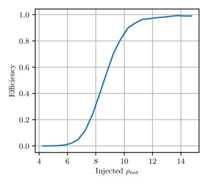
Figure 5: Efficiency of recovering injections at different injected SNRs

IV.5 Sensitivity estimate

The sensitivity of our new pipeline is demonstrated in Fig. 4 and Fig. 5. Fig. 4 shows the distribution of all the injected events by SNR with a network SNR of 12 contour, and detector SNR of 7 contours added. This figure shows that the majority of loud injected events were recovered by our pipeline, with 70 missed in the region with network SNR above 12 and detector SNRs greater than 7. Only nine of these missed injections are because the pipeline could not adequately recover the injections. This shows that the pipeline only very rarely gets stuck at local peaks, instead of finding the global maxima, which will correspond to the injected signal. It is possible that as we move to a lower mass parameter space, the frequecy of such occurrences will increase. All of the loud missed events are discussed in more detail in Appendix B.

Fig. 5 shows the efficiency of the pipeline as a function of the injected network snr of the synthetic gravitational wave set described in section C. This plot shows that without any data cleaning implementation, almost 90% of events at SNR 10 are recovered by the pipeline while that percentage only increases with the SNR and plateaus just short of 100% around SNR 13.

V Conclusion

In this paper, we have described in detail a novel gravitational wave detection algorithm. This algorithm searches stochastically over the chosen parameter space, saving the time and computing power required to generate large banks of template waveforms. The algorithm samples the parameter space by making jumps with a pre-estimated mismatch between templates informed by the parameter space metric and keeping those points which have a higher SNR. This method is shown to be of comparable accuracy in the recovery of gravitational wave events at high masses as current template-based pipelines.

To demonstrate the validity of this method, we have presented an analysis of approximately one month of LIGO data from July 27 00:00 2017 UTC – Aug 25 22:00 2017 UTC exploring the binary black hole parameter space. We recovered six known gravitational wave candidate events to within tens of milliseconds of previously reported coalescence times, as well as two gravitational wave candidates previously reported.

Additionally, we conducted an injection campagin of compact binary mergers to prove the sensitivity of the pipeline to binary black hole merger events. We recovered almost 90% of events with SNR 10 and an increasing percentage at higher SNRs that plateaus just below 100% at SNR 13. The majority of the missing loud injections were due to the presence of glitches near the injected events.

In the future, we plan to extend our method to all regions of the parameter space. We expect that even though the algorithm will scale similarly to any search using template banks at lower mass, it will still retain its other advantages, such as simpler workflow and ease of setup. We plan to make our method competitive with other searches like GstLAL for LIGO’s fourth observing run. It remains an open project to get good convergence during the sampling process for all regions of the parameter space.

Appendix A Data release details and code versions

A tarball containing the source code and data files necessary to reproduce the results and plots in this paper can be found at https://dcc.ligo.org/T2100321. Instructions for installing the code and for using it to create the plots and results can be found in README.md inside the source_code directory in the tarball.

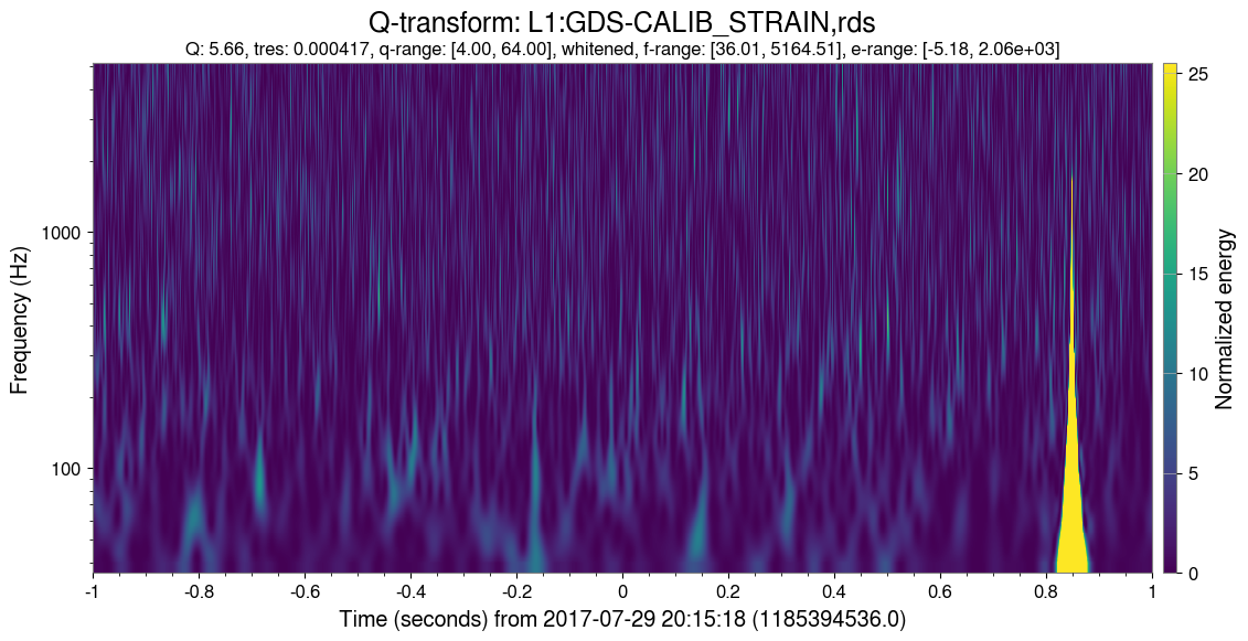
Figure 6: An example of a Q-transform plot showing a glitch in Livingston, causing a simultaneous injection to be missed

Appendix B Follow-up of missed injections

In this appendix, we will discuss the particularly loud injections which were not recovered during the simulation mode of the pipeline. An injection is deemed to be recovered, if it was assigned a log-likelihood ratio, $\mathcal{L}$ of 35 or greater. Out of the 112526 injections, 65361 were missed. Most of these (65291 out of 65361) were missed because the injected SNR was too low for them to be recovered significantly. Some, however had a high injected SNR and were still missed. We will discuss the reasons for the same, for missed injections with network SNR above 12 and detector SNRs greater than 7. These injections are shown in Fig. 4, of which there are 70. Out of these, 33 were missed due to the data containing a glitch simultaneous to the injection, causing the glitch rejection mechanism to reject that part of the data. The existence of a glitch in the data was verified by creating Q-transform plots of the data window. An example of such a glitch is shown in Fig. 6. Out of the remaining 37 loud missed injections, 28 fell into the glitch region as defined in Section III-D.6, and hence were rejected. The pipeline failed to recover only 9 injections out of the original 112526. However, such problematic injections can be recovered by increasing $N_{k}$, the number of samples to reject at each level, $k$, before moving on to the next, at the cost of the run-time of the pipeline.

References

- Abbott et al. (2016a) B. P. Abbott et al. (LIGO Scientific, Virgo), Phys. Rev. Lett. 116, 061102 (2016a), arXiv:1602.03837 [gr-qc] .
- Abbott et al. (2016b) B. P. Abbott et al. (LIGO Scientific, Virgo), Phys. Rev. Lett. 116, 241103 (2016b), arXiv:1606.04855 [gr-qc] .
- Abbott et al. (2019) B. P. Abbott et al. (LIGO Scientific, Virgo), Phys. Rev. X 9, 031040 (2019), arXiv:1811.12907 [astro-ph.HE] .
- Abbott et al. (2020a) R. Abbott, T. Abbott, S. Abraham, F. Acernese, K. Ackley, A. Adams, C. Adams, R. Adhikari, V. Adya, C. Affeldt, et al., arXiv preprint arXiv:2010.14527 (2020a).
- Abbott et al. (2021a) R. Abbott, T. Abbott, F. Acernese, K. Ackley, C. Adams, N. Adhikari, R. Adhikari, V. Adya, C. Affeldt, D. Agarwal, et al., arXiv preprint arXiv:2108.01045 (2021a).
- Collaboration et al. (2021) T. L. S. Collaboration, the Virgo Collaboration, the KAGRA Collaboration, R. Abbott, T. D. Abbott, F. Acernese, K. Ackley, C. Adams, N. Adhikari, R. X. Adhikari, et al., “Gwtc-3: Compact binary coalescences observed by ligo and virgo during the second part of the third observing run,” (2021), arXiv:2111.03606 [gr-qc] .
- Abbott et al. (2017) B. P. Abbott et al. (LIGO Scientific, Virgo), Phys. Rev. Lett. 119, 161101 (2017), arXiv:1710.05832 [gr-qc] .
- Abbott et al. (2020b) B. P. Abbott et al. (LIGO Scientific, Virgo), (2020b), arXiv:2001.01761 [astro-ph.HE] .
- Abbott et al. (2021b) R. Abbott, T. Abbott, S. Abraham, F. Acernese, K. Ackley, A. Adams, C. Adams, R. Adhikari, V. Adya, C. Affeldt, et al., The Astrophysical Journal Letters 915, L5 (2021b).
- Trovato (2020) A. Trovato (Ligo Scientific, The Virgo), Proceedings, The New Era of Multi-Messenger Astrophysics (ASTERICS 2019): Groningen, Netherlands, March 25-29, 2019, PoS Asterics2019, 082 (2020).
- Zackay et al. (2019a) B. Zackay, L. Dai, T. Venumadhav, J. Roulet, and M. Zaldarriaga, (2019a), arXiv:1910.09528 [astro-ph.HE] .
- Venumadhav et al. (2019a) T. Venumadhav, B. Zackay, J. Roulet, L. Dai, and M. Zaldarriaga, (2019a), arXiv:1904.07214 [astro-ph.HE] .
- Zackay et al. (2019b) B. Zackay, T. Venumadhav, L. Dai, J. Roulet, and M. Zaldarriaga, Phys. Rev. D100, 023007 (2019b), arXiv:1902.10331 [astro-ph.HE] .
- Venumadhav et al. (2019b) T. Venumadhav, B. Zackay, J. Roulet, L. Dai, and M. Zaldarriaga, Phys. Rev. D100, 023011 (2019b), arXiv:1902.10341 [astro-ph.IM] .
- Nitz et al. (2021) A. H. Nitz, C. D. Capano, S. Kumar, Y.-F. Wang, S. Kastha, M. Schäfer, R. Dhurkunde, and M. Cabero, “3-ogc: Catalog of gravitational waves from compact-binary mergers,” (2021), arXiv:2105.09151 [astro-ph.HE] .
- Abbott et al. (2021c) R. Abbott, T. D. Abbott, S. Abraham, F. Acernese, K. Ackley, A. Adams, C. Adams, R. X. Adhikari, V. B. Adya, C. Affeldt, and et al., The Astrophysical Journal Letters 915, L5 (2021c).
- Finn and Chernoff (1993) L. S. Finn and D. F. Chernoff, Phys. Rev. D47, 2198 (1993), arXiv:gr-qc/9301003 [gr-qc] .
- Owen (1996) B. J. Owen, Phys. Rev. D 53, 6749 (1996).
- Owen and Sathyaprakash (1999) B. J. Owen and B. S. Sathyaprakash, Phys. Rev. D60, 022002 (1999), arXiv:gr-qc/9808076 [gr-qc] .
- Allen et al. (2012) B. Allen, W. G. Anderson, P. R. Brady, D. A. Brown, and J. D. E. Creighton, Phys. Rev. D85, 122006 (2012), arXiv:gr-qc/0509116 [gr-qc] .
- Cannon et al. (2012) K. Cannon et al., Astrophys. J. 748, 136 (2012), arXiv:1107.2665 [astro-ph.IM] .
- Babak et al. (2013) S. Babak, R. Biswas, P. Brady, D. A. Brown, K. Cannon, C. D. Capano, J. H. Clayton, T. Cokelaer, J. D. Creighton, T. Dent, et al., Physical Review D 87, 024033 (2013).
- Nitz et al. (2017) A. H. Nitz, T. Dent, T. Dal Canton, S. Fairhurst, and D. A. Brown, Astrophys. J. 849, 118 (2017), arXiv:1705.01513 [gr-qc] .
- Adams et al. (2016) T. Adams, D. Buskulic, V. Germain, G. M. Guidi, F. Marion, M. Montani, B. Mours, F. Piergiovanni, and G. Wang, Class. Quant. Grav. 33, 175012 (2016), arXiv:1512.02864 [gr-qc] .
- Harry et al. (2009) I. W. Harry, B. Allen, and B. Sathyaprakash, Physical Review D 80, 104014 (2009).
- Ajith et al. (2014) P. Ajith, N. Fotopoulos, S. Privitera, A. Neunzert, N. Mazumder, and A. Weinstein, Physical Review D 89, 084041 (2014).
- Harry et al. (2016) I. Harry, S. Privitera, A. Bohé, and A. Buonanno, Physical Review D 94, 024012 (2016).
- Cornish and Crowder (2005) N. J. Cornish and J. Crowder, Physical Review D 72, 043005 (2005).
- Veitch et al. (2015) J. Veitch, V. Raymond, B. Farr, W. Farr, P. Graff, S. Vitale, B. Aylott, K. Blackburn, N. Christensen, M. Coughlin, W. Del Pozzo, F. Feroz, J. Gair, C.-J. Haster, V. Kalogera, T. Littenberg, I. Mandel, R. O’Shaughnessy, M. Pitkin, C. Rodriguez, C. Röver, T. Sidery, R. Smith, M. Van Der Sluys, A. Vecchio, W. Vousden, and L. Wade, Phys.Rev.D 91, 042003 (2015), arXiv:1409.7215 [gr-qc] .
- Ashton et al. (2019) G. Ashton, M. Hübner, P. D. Lasky, C. Talbot, K. Ackley, S. Biscoveanu, Q. Chu, A. Divakarla, P. J. Easter, B. Goncharov, et al., The Astrophysical Journal Supplement Series 241, 27 (2019).
- et al. (LIGO Scientific Collaboration and Collaboration) R. A. et al. (LIGO Scientific Collaboration and V. Collaboration), SoftwareX 13, 100658 (2021).
- Messick et al. (2017) C. Messick et al., Phys. Rev. D95, 042001 (2017), arXiv:1604.04324 [astro-ph.IM] .
- Sachdev et al. (2019) S. Sachdev et al., (2019), arXiv:1901.08580 [gr-qc] .
- Cannon et al. (2021) K. Cannon, S. Caudill, C. Chan, B. Cousins, J. D. Creighton, B. Ewing, H. Fong, P. Godwin, C. Hanna, S. Hooper, et al., SoftwareX 14, 100680 (2021).
- (35) “GstLAL software: git.ligo.org/lscsoft/gstlal,” .
- osg (2021) “Open science grid: Introduction,” (2021).
- Cannon et al. (2015) K. Cannon, C. Hanna, and J. Peoples, (2015), arXiv:1504.04632 [astro-ph.IM] .
- Cannon et al. (2013) K. Cannon, C. Hanna, and D. Keppel, Phys. Rev. D88, 024025 (2013), arXiv:1209.0718 [gr-qc] .
- (39) “Lvc algorithm library software: git.ligo.org/lscsoft/lalsuite,” .
- Ashton et al. (2021) G. Ashton, S. Thiele, Y. Lecoeuche, J. McIver, and L. K. Nuttall, “Parameterised population models of transient non-gaussian noise in the ligo gravitational-wave detectors,” (2021), arXiv:2110.02689 [gr-qc] .
- Davis et al. (2020) D. Davis, L. V. White, and P. R. Saulson, Classical and Quantum Gravity 37, 145001 (2020).
- Fairhurst (2009) S. Fairhurst, New Journal of Physics 11, 123006 (2009).
- Hanna et al. (2020) C. Hanna et al., Phys. Rev. D101, 022003 (2020), arXiv:1901.02227 [gr-qc] .
- Nitz et al. (2019) A. H. Nitz, T. Dent, G. S. Davies, S. Kumar, C. D. Capano, I. Harry, S. Mozzon, L. Nuttall, A. Lundgren, and M. Tápai, (2019), arXiv:1910.05331 [astro-ph.HE] .