Towards a numerical solution of the bosonic master-field equation of the IIB matrix model

Abstract

A direct algebraic solution has been obtained from the full bosonic master-field equation of the IIB matrix model for low dimensionality $D=3$ and small matrix size $N=3$. A different method is needed for larger values of $D$ and $N$. Here, we explore an indirect numerical approach and obtain an approximate numerical solution for the nontrivial case $(D,\,N)=(10,\,4)$ with a complex Pfaffian. We also present a suggestion for numerical calculations at larger values of $N$.

Acta Phys. Pol. B 53, 1–A5 (2022) arXiv:2110.15309

04.20.Cv, 11.25.-w, 11.25.Yb, 98.80.Bp

1 Introduction

It has been argued that the bosonic large-$N$ master field [1, 2] of the IIB matrix model [3, 4] can give rise to an emergent classical spacetime [5] (see also Ref. [6] for further work on cosmology and Ref. [7] for a brief review). The crucial point, now, is that the bosonic master field is essentially determined by an algebraic equation and not a differential equation.

In a first paper [8], we have considered this algebraic equation with the effects of fermions removed altogether. In a subsequent paper [9], we turned to the full algebraic equation with the effects of fermions included and were able to obtain a solution for dimensionality $D=3$ and matrix size $N=3$.

This result for $(D,\,N)=(3,\,3)$ is certainly gratifying, but it appears that, with the same type of algebraic method, progress to larger values of $D$ and $N$ does not seem feasible. A different method is required to, ultimately, reach the parameters $D=10$ and $N\gg 1$ of the genuine IIB matrix model. The present paper explores an indirect numerical approach which looks promising (the meaning of the qualification “indirect” will be explained later).

Before we get started, we would like to clarify the scope of the present article. The numerical results to be given in Sec. 5 are only indicative. The importance of the $(D,\,N)=(10,\,4)$ numerical results, in particular, is to show that the proposed method works. As such, these numerical results need to be viewed as a preparation for future work with more powerful computers, which are needed anyway for reaching larger values of $N$.

2 Algebraic equation

As the present paper is solely devoted to obtaining solutions of a particular algebraic equation, let us immediately give that equation (some background on the origin and meaning of the equation will be given in Sec. 3). Specifically, this algebraic equation for $D$ traceless Hermitian matrices $\widehat{a}^{\;\mu}$ of dimension $N\times N$ reads

$$i\,\big{(}\widehat{p}_{k}-\widehat{p}_{l}\big{)}\;\widehat{a}^{\;\mu}_{\;kl}+\Big{[}\widehat{a}^{\,\nu},\,\big{[}\widehat{a}^{\,\nu},\,\widehat{a}^{\;\mu}\big{]}\Big{]}_{kl}-\frac{1}{\mathcal{P}\left(\widehat{a}\,\right)}\;\frac{\partial\,\mathcal{P}\left(\widehat{a}\,\right)}{\partial\,\widehat{a}^{\;\mu}_{\;lk}}-\widehat{\eta}^{\;\mu}_{\;kl}=0\,,$$ (1a)

$$\mathcal{P}\left(\widehat{a}\,\right)=\text{homogeneous polynomial of order $K$}\,,$$ (1b)

$$K\equiv\big{(}D-2\big{)}\,\big{(}N^{2}-1\big{)}\,,$$ (1c)

$$D=10\,,\quad N\gg 1\,,$$ (1d)

with matrix indices $k,\,l$ running over $\{1,\,\ldots\,,\,N\}$ and directional indices $\mu,\,\nu$ running over $\{1,\,\ldots\,,\,D\}$, while $\nu$ in (1a) is implicitly summed over. The $\widehat{p}_{k}$ in (1a) are uniform random numbers and the $\widehat{\eta}^{\;\mu}_{\;kl}$ Gaussian random numbers (these numbers can be fixed once and for all, provided $N$ is large enough; see Sec. 4.2 for further details). There is an explicit expression for the Pfaffian $\mathcal{P}$ to be discussed later.

The algebraic equation (1a) is quite a challenge for mathematics and computational science. But why is that equation also of interest to physics? Well, the answer is that its solution may contain information about the emergence of spacetime and the birth of the Universe. As promised above, we will give some background in the next section, but the main focus of the present paper is really on obtaining solutions of the above algebraic equation.

3 Background

The algebraic equation of interest arises from the IKKT matrix model [3]. That model is also known as the IIB matrix model [4], because the matrix model reproduces the structure of the light-cone type-IIB superstring field theory.

The IIB matrix model of Kawai and collaborators [3, 4] has a finite number of $N\times N$ traceless Hermitian matrices: ten bosonic matrices $A^{\mu}$ and eight fermionic Majorana–Weyl matrices $\Psi_{\alpha}$. The partition function $Z$ of the IIB matrix model is defined by the following “path” integral:

$$Z=\int dA\,d\Psi\;e^{\displaystyle{-S_{\text{bos}}(A)-S_{\text{ferm}}(\Psi,\,A)}}.$$ (2)

Here, the bosonic action $S_{\text{bos}}(A)$ is quartic in $A$ (the trace of the square of Yang–Mills-type commutators) and the fermionic action $S_{\text{ferm}}(\Psi,\,A)$ is quadratic in $\Psi$ and linear in $A$ (a Dirac-type term without derivatives but with Yang–Mills-type commutators). In a symbolic notation, the fermionic action reads

$$S_{\text{ferm}}=\overline{\Psi}\,\mathcal{M}(A)\,\Psi\,.$$ (3)

The precise definition of the measure in (2) and further details are summarized in Ref. [9].

The fermionic matrices $\Psi$ in (2) can be integrated out exactly (Gaussian integrals) and there results a Pfaffian:

$$\text{Pf}\big{[}\mathcal{M}(A)\big{]}\equiv\mathcal{P}(A)\,,$$ (4)

with further details collected in App. A. The final expression for the partition function then reads

$$Z=\int dA\;\mathcal{P}(A)\;e^{\displaystyle{-S_{\text{bos}}(A)}}=\int dA\;e^{\displaystyle{-S_{\text{eff}}(A)}}\,,$$ (5a)

$$S_{\text{eff}}(A)=S_{\text{bos}}(A)-\log\,\mathcal{P}(A)\,.$$ (5b)

For the bosonic observable

$$w^{\mu_{1}\,\ldots\,\mu_{m}}\equiv\text{Tr}\,\big{(}A^{\mu_{1}}\cdots\,A^{\mu_{m}}\big{)}\,,$$ (6)

and arbitrary strings thereof, the expectation values are defined by the same integral as in (5a):

$$\langle w^{\mu_{1}\,\ldots\,\mu_{m}}\>w^{\nu_{1}\,\ldots\,\nu_{n}}\,\cdots\,w^{\omega_{1}\,\ldots\,\omega_{z}}\rangle$$

$$=\frac{1}{Z}\int dA\,\big{(}w^{\mu_{1}\,\ldots\,\mu_{m}}\>w^{\nu_{1}\,\ldots\,\nu_{n}}\,\cdots\,w^{\omega_{1}\,\ldots\,\omega_{z}}\big{)}\,e^{\displaystyle{-\,S_{\text{eff}}}}\,.$$ (7)

At this moment, we can make a trivial but important observation: the matrices of the IIB matrix model (2) have no spacetime dependence (for this reason, we have used quotation marks in the terminology “path” integral). In fact, the IIB matrix model just gives numbers, $Z$ and the expectation values $\langle w\>w\,\cdots\,w\rangle$, while the matrices $A^{\mu}$ and $\Psi_{\alpha}$ in the “path” integral are merely integration variables. In addition, there is no small dimensionless parameter to motivate a saddle-point approximation. So, how does the classical spacetime emerge? Recently, we have suggested [5] to revisit an old idea, the large-$N$ master field of Witten [1, 2], for a possible origin of classical spacetime in the context of the IIB matrix model.

According to Witten [1], the large-$N$ factorization of the expectation values (3) implies that the path integrals are saturated by a single configuration, the so-called master field $\widehat{A}^{\,\mu}$. To leading order in $N$, the expectation values are then given by

$$\langle w^{\mu_{1}\,\ldots\,\mu_{m}}\,w^{\nu_{1}\,\ldots\,\nu_{n}}\cdots\,w^{\omega_{1}\,\ldots\,\omega_{z}}\rangle\,\stackrel{{\scriptstyle N}}{{=}}\,\widehat{w}^{\,\mu_{1}\,\ldots\,\mu_{m}}\,\widehat{w}^{\,\nu_{1}\,\ldots\,\nu_{n}}\cdots\,\widehat{w}^{\,\omega_{1}\,\ldots\,\omega_{z}},$$ (8a)

$$\widehat{w}^{\,\mu_{1}\,\ldots\,\mu_{m}}\equiv\text{Tr}\,\big{(}\widehat{A}^{\,\mu_{1}}\cdots\,\widehat{A}^{\,\mu_{m}}\big{)}\,.$$ (8b)

Hence, we do not have to perform the integral on the right-hand side of (3): we only need ten traceless Hermitian matrices $\widehat{A}^{\,\mu}$ to get all these expectation values from the simple procedure of replacing each $A^{\,\mu}$ in the observables by the corresponding $\widehat{A}^{\,\mu}$.

Now, the meaning of our previous suggestion is clear: classical spacetime may reside in the bosonic master-field matrices $\widehat{A}^{\,\mu}$ of the IIB matrix model. The heuristics is as follows [7]:

• The expectation values $\left\langle w^{\mu_{1}\,\ldots\,\mu_{m}}\,\cdots\,w^{\omega_{1}\,\ldots\,\omega_{z}}\right\rangle$ from (3) correspond to an infinity of real numbers and give a large part of the information content of the IIB matrix model (but, obviously, not all the information).

• That same information is encoded in the master-field matrices $\widehat{A}^{\,\mu}$, which, to leading order in $N$, give precisely the same numbers by the products $\widehat{w}^{\,\mu_{1}\,\ldots\,\mu_{m}}\,\cdots\,$ $\widehat{w}^{\,\omega_{1}\,\ldots\,\omega_{z}}$, where $\widehat{w}$ is simply the observable $w$ evaluated for $\widehat{A}$.

• From these master-field matrices $\widehat{A}^{\,\mu}$, it is possible to extract the points and the metric of an emergent classical spacetime (as mentioned before, the original matrices $A^{\,\mu}$ are merely integration variables).

Assuming that the matrices $\widehat{A}^{\,\mu}$ of the IIB-matrix-model master field are known and that they are approximately band-diagonal (as suggested by the numerical results of Ref. [10, 11, 12] and references therein), it is relatively easy [5] to extract a discrete set of spacetime points $\{\widehat{x}^{\,\mu}_{k}\}$ and an interpolating inverse metric $g^{\mu\nu}(x)$. The metric $g_{\mu\nu}(x)$ is obtained as matrix inverse of $g^{\mu\nu}(x)$.

But, instead of just assuming the matrices $\widehat{A}^{\,\mu}$, we want to calculate them. And, for that, we need an equation.

4 Master-field equation: General discussion

4.1 Preliminary remarks

Let us start with some good news: the master-field equation has already been established, nearly 40 years ago, by Greensite and Halpern [2]. They write in the first line of their abstract: “We derive an exact algebraic (master) equation for the euclidean master field of any large-$N$ matrix theory, including quantum chromodynamics.” Now, “any” means “any” and we may as well consider the large-$N$ IIB matrix theory [3, 4].

A side remark is that the sentence quoted above is, perhaps, a little bit too general. For example, an obvious restriction would be the restriction to any consistent large-$N$ matrix theory, where the additional adjective “consistent” implies that the theory makes sense physically (being, for example, causal and reflection-positive/unitary). In any case, the IIB matrix model is certainly a good candidate for a consistent large-$N$ matrix theory.

4.2 Bosonic master-field equation

Building on the work by Greensite and Halpern [2], we then have the IIB-matrix-model bosonic master field in a “quenched” form [5]:

$$\widehat{A}^{\;\mu}_{\;kl}=e^{\displaystyle{i\,\widehat{p}_{k}\,\tau_{\text{eq}}}}\;\,\widehat{a}^{\;\mu}_{\;kl}\;\,e^{\displaystyle{-i\,\widehat{p}_{l}\,\tau_{\text{eq}}}}\,.\vspace*{-0mm}$$ (9a)

Here, the $$\widehat{p}_{k} \tau_{\text{eq}} \tau \tau \widehat{a}^{\;\mu}$$ are dimensionless random constants (see below) and the dimensionless time must have a sufficiently large value in order to represent an equilibrium situation ( is the fictitious Langevin time of the stochastic-quantization procedure). The -independent matrix on the right-hand side of (9a) solves the following algebraic equation [5]:

$$i\,\big{(}\widehat{p}_{k}-\widehat{p}_{l}\big{)}\;\widehat{a}^{\;\mu}_{\;kl}+\frac{\partial\,S_{\text{eff\,}}\left(\widehat{a}\,\right)}{\partial\,\widehat{a}_{\mu\;lk}}-\widehat{\eta}^{\;\mu}_{\;kl}=0\,,\vspace*{-0mm}$$ (9b)

in terms of the effective action $S_{\text{eff\,}}\left(\widehat{a}\,\right)$ from (5b), the master momenta $\widehat{p}_{k}$ (real uniform random numbers), and the master noise matrices $\widehat{\eta}^{\;\mu}_{\;kl}$ [using real Gaussian random numbers for the corresponding coefficients $\widehat{\eta}^{\;\mu}_{\;c}$ with Lie-algebra index $c$, where the expansion is similar to (25) in App. A ].

Further details on the interpretation of (9a) and (9b) can be found in Sec. 3.2 of Ref. [9]. At this moment, we like to emphasize one point (already briefly mentioned in Sec. 2): the random numbers $\widehat{p}_{k}$ and $\widehat{\eta}^{\;\mu}_{\;kl}$ can be fixed once and for all (assuming that $N$ is large enough) and these random numbers are called the master momenta and noise. This observation implies that, at large $N$, it suffices to solve the algebraic equation (9b) with a particular realization of random numbers $\widehat{p}_{k}$ and $\widehat{\eta}^{\;\mu}_{\;kl}$, and this is the strategy employed in our previous papers [8, 9] and the present one.

The algebraic equation (9b) is, of course, precisely (1a).

4.3 Simplified equation

The algebraic equation (1a) is truly formidable and it makes sense to first consider the simplified equation without Pfaffian term [8]:

$$i\,\big{(}\widehat{p}_{k}-\widehat{p}_{l}\big{)}\;\widehat{a}^{\;\mu}_{\;kl}+\Big{[}\widehat{a}^{\,\nu},\,\big{[}\widehat{a}^{\,\nu},\,\widehat{a}^{\;\mu}\big{]}\Big{]}_{kl}-\widehat{\eta}^{\;\mu}_{\;kl}=0\,.$$ (10)

The matrices $\widehat{a}^{\;\mu}$ are $N\times N$ traceless Hermitian matrices and the number of variables is

$$N_{\text{var}}=D\,\big{(}N^{2}-1\big{)}\,,$$ (11)

which grows rapidly with increasing $N$. The simplified equation (10) is essentially a cubic polynomial. Remark also that the simplified equation (10) differs from the one in Ref. [8] by the sign of the double commutator, but this can be compensated by a redefinition of $\widehat{p}_{k}$ and $\widehat{\eta}^{\;\mu}_{\;kl}$.

It appears impossible to obtain a general analytic solution of (10) in terms of the master constants $\widehat{p}_{k}$ and $\widehat{\eta}^{\;\mu}_{\;kl}$. Instead, we have obtained solutions [8] for $(D,\,N)=(2,\,4)$ and $(D,\,N)=(2,\,6)$ by taking a particular realization of the random master constants (other realizations give similar results). As our focus will be on $N=4$ in the following, we briefly review here the results of the simplified equation (10) for $(D,\,N)=(2,\,4)$.

Taking a particular realization (the “alpha-realization”) of the 4 pseudorandom numbers for the master momenta and the 30 pseudorandom numbers for the master noise (they are given by Eqs. (16abc) in Ref. [8], with overall minus signs added), we have obtained an explicit solution $\widehat{a}^{\,1}_{\alpha\text{-sol}}$ and $\widehat{a}^{\,2}_{\alpha\text{-sol}}\,$ as given by Eqs. (17ab) in Ref. [8]. For the absolute values of these matrix entries, the density plots are shown in the first two panels of Fig. 1. There is no obvious band-diagonal structure.

Next, change the basis, in order to diagonalize and order the $\mu=1$ matrix. This produces the matrices $\widehat{a}^{\;\prime\,1}_{\alpha\text{-sol}}$ and $\widehat{a}^{\;\prime\,2}_{\alpha\text{-sol}}$ as given by Eqs. (21ab) in Ref. [8]. For the absolute values of these new matrix entries, the density plots are shown in the last two panels of Fig. 1. There appears a clear band-diagonal structure in $\widehat{a}^{\;\prime\,2}_{\alpha\text{-sol}}$, which is a nontrivial result.

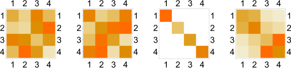
Figure 1: (color) From left to right, density plots of the matrices $\text{Abs}\left[\widehat{a}^{\,1}_{\alpha\text{-sol}}\right]$, $\text{Abs}\left[\widehat{a}^{\,2}_{\alpha\text{-sol}}\right]$, $\text{Abs}\left[\widehat{a}^{\;\prime\,1}_{\alpha\text{-sol}}\right]$, and $\text{Abs}\left[\widehat{a}^{\;\prime\,2}_{\alpha\text{-sol}}\right]$, as obtained in Sec. 4.1 of Ref. [8] from the simplified algebraic equation (10) for $(D,\,N)=(2,\,4)$ and a particular choice (labelled “$\alpha$”) of master momenta and master noise.

As mentioned in Sec. 3, the diagonal/band-diagonal structure of the master-field matrices allows for the extraction of a classical spacetime, but it remains to demonstrate that dynamical fermions do not spoil this structure.

4.4 Full equation rewritten with a trace term

We now look for solutions of the full bosonic master-field equation (1a), with dynamic fermions included, but, first, only for rather small values of $D$ and $N$.

The Pfaffian is a $K$-th order homogenous polynomial, denoted symbolically by $P_{K}(A)$, with $K=(D-2)\,(N^{2}-1)$. Further details are given in App. A. The basic structure of the algebraic equation (1a) is then as follows:

$$P_{1}^{(\,\widehat{p}\,)}\left(\widehat{a}\,\right)+P_{3}\left(\widehat{a}\,\right)+\frac{P_{K-1}\left(\widehat{a}\,\right)}{P_{K}\left(\widehat{a}\,\right)}+P_{0}^{(\,\widehat{\eta}\,)}\left(\widehat{a}\,\right)=0\,,\vspace*{-0mm}$$ (12)

where the suffixes on $P_{0}$ and $P_{1}$ indicate their respective dependence on the master noise $\widehat{\eta}^{\;\mu}_{kl}$ and the master momenta $\widehat{p}_{k}$. Multiplying (12) by $P_{K}\left(\widehat{a}\,\right)$, we get a polynomial equation of order $K+3$ with the following structure:

$$P_{K+1}^{(\,\widehat{p}\,)}\left(\widehat{a}\,\right)+P_{K+3}\left(\widehat{a}\,\right)+P_{K-1}\left(\widehat{a}\,\right)+P_{K}^{(\,\widehat{\eta}\,)}\left(\widehat{a}\,\right)=0\,.\vspace*{-0mm}$$ (13)

For the case $\{D,\,N\}=\{3,\,3\}$, there is an explicit algebraic result for the Pfaffian [13]. Taking a particular realization of the random constants (other realizations give similar results), we have established [9] the existence of several solutions of the full bosonic master-field equation (1a). Moreover, there is a mild diagonal/band-diagonal structure, but the value $N=3$ is too small for definitive statements.

These $(D,\,N)=(3,\,3)$ results were obtained by a direct algebraic calculation and it would seem difficult to go to larger values of $D$ and $N$. But perhaps there can be progress with a numerical approach. The idea [15] is to use the fact that the square of the Pfaffian of the skew-symmetric matrix $\mathcal{M}=\mathcal{M}\left(\widehat{a}\,\right)$ equals its determinant,

$$\big{[}\text{Pf}(\mathcal{M})\big{]}^{2}=\det\mathcal{M}\,,\vspace*{-0mm}$$ (14)

so that we can write the variational term in the algebraic equation (1a) as a trace,

$$\frac{\delta\,\text{Pf}(\mathcal{M})}{\text{Pf}(\mathcal{M})}=\frac{1}{2}\;\frac{\delta\det\mathcal{M}}{\det\mathcal{M}}=\frac{1}{2}\;\text{Tr}\big{[}\mathcal{M}^{-1}\delta\,\mathcal{M}\big{]}\,,\vspace*{-0mm}$$ (15)

and this trace can be readily evaluated numerically (as was done in Ref. [12]). Just to be clear, it is the third term on the left-hand side of (1a) that is replaced by a term involving the trace, according to (15).

We will call the resulting calculation an indirect numerical calculation, where the qualification “indirect” is meant to show that the Pfaffian is not directly considered but rather its relative variation written as the trace term (15) with the matrix $\mathcal{M}_{A,\,B}$ from App. A. First results from this indirect numerical calculation will be presented in Sec. 5.

5 Numerical results from the full algebraic equation

5.1 Cases $(D,\,N)=(3,\,3)$ and $(D,\,N)=(10,\,3)$

We have performed numerical calculations of the full algebraic equation (1a) with the trace term (15) for three cases: $(D,\,N)=(3,\,3)$, $(D,\,N)=(10,\,3)$, and $(D,\,N)=(10,\,4)$. Some details of the calculations are listed in Table 1.

The numerical results of the first two rows in Table 1 were obtained from the NMinimize routine of Mathematica 12.1 (cf. Ref. [16]) with the downhill-simplex method of Nelder and Mead [17, 18]. Our main interest is, however, in the $(D,\,N)=(10,\,4)$ case and we will discuss that case in the next subsection.

Table 1: Numerical calculations of the full bosonic master-field equation (1a) using the identity (15). The number of variables is given by $N_{\text{var}}=D\,(N^{2}-1)$ and the order of the Pfaffian by $K=(D-2)\,(N^{2}-1)$.

	$N_{\text{var}}$	$K$	calculational details a
$(D,\,N)=(3,\,3)$	24	8	single-processor, $\text{O}(\text{hr})$ b
$(D,\,N)=(10,\,3)$	80	64	single-processor, $\text{O}(\text{day})$
$(D,\,N)=(10,\,4)$	150 c	120	6-kernel, $\text{O}(\text{month})$

^a for a Lenovo T15p notebook with an Intel Core i7-10750H processor (6 kernels, 12
^a threads, 12 MB cache, 2.6 – 5.0 GHz clock frequency) running Mathematica 12.1.
^b reproducing the previous algebraic results [9].
^c complex variables in the matrix solution, as the Pfaffian $\mathcal{P}\left(\widehat{a}\,\right)$ is complex (cf. App. A).

5.2 Case $(D,\,N)=(10,\,4)$

The downhill-simplex method used for $(D,\,N)=(3,\,3)$ and $(D,\,N)=(10,\,3)$ is, without further modifications, no longer suitable for the 300 real variables of the present case,

$$(D,\,N)=(10,\,4)\,.$$ (16)

Instead, we have used a simple random-step procedure, which could be partially parallelized. In this way, we have obtained an approximate numerical solution. A numerical solution is, of course, always “approximate,” but occasionally we prefer to emphasize this fact by use of the adjective.

Before we describe the obtained results, we need to specify the particular realization (the “$\kappa$-realization”) of the pseudorandom numbers entering the algebraic equation (1a). As this involves 154 real numbers, the details are rather cumbersome and are relegated to App. B. Other realizations of the pseudorandom numbers (the $\lambda$, $\mu$, $\nu$, $\ldots$ realizations) are expected to give similar results, according to our previous results [8, 9].

The calculation follows the same procedure as in our earlier work, namely the numerical minimization of a nonnegative function $f_{\text{penalty}}$ that will be defined shortly. But the calculation for the case (16) is hard with many variables and a high-order Pfaffian. The main difficulty is that, for a computer as described in Footnote a of Table 1, the evaluation of $f_{\text{penalty}}$ at a single point in the 300-dimensional configuration space takes a long time, about 90 seconds [which is approximately ten times more than for the $(D,\,N)=(10,\,3)$ calculation]. Furthermore, the $f_{\text{penalty}}$ valley appears to be long, narrow, and winding (at least, for the used coordinates $\widehat{r}_{\mu}^{\;c}$ and $\widehat{s}_{\mu}^{\;c}$, to be defined shortly).

As the Pfaffian term in the algebraic equation is complex, we must allow for complex variables in the solution:

$$\widehat{a}_{\mu}^{\;c}=\widehat{r}_{\mu}^{\;c}+i\;\widehat{s}_{\mu}^{\;c}\in\mathbb{C}\,,$$ (17)

with real numbers $\widehat{r}_{\mu}^{\;c}$ and $\widehat{s}_{\mu}^{\;c}$. In this way, we have obtained a series of approximate numerical solutions of the algebraic equation (1a) with the identity (15) and the $\kappa$-realization of pseudorandom constants. A selection of these approximate numerical solutions is shown in Table 2, where the caption defines the function $f_{\text{penalty}}$, as well as another diagnostic quantity. Specifically, we will discuss the approximate numerical solution from the last row of Table 2 and denote this particular solution by “$\kappa\text{-num-\text@underline{sol}}$”. We, then, have 300 real numbers defining the following matrices:

$$\widehat{a}^{\,\mu}_{\kappa\text{-num-\text@underline{sol}}}\,,\;\;\;\text{for}\;\;\;\mu=1,\,\ldots\,,10\,.$$ (18)

With complex coefficients $\widehat{a}_{\mu}^{\;c}$, these (approximate) master-field matrices are no longer Hermitian. The situation is perhaps analogous to that of complex saddle-points appearing for a real problem. Our interpretation is that these (approximate) master-field matrices carry information both in their Hermitian and anti-Hermitian parts.

Table 2: Approximate numerical solutions of the full $(D,\,N)=(10,\,4)$ bosonic master-field equation (1a) with the identity (15) and the pseudorandom constants given in App. B. The complex residues of the 150 component equations $\text{eq-}\widehat{a}_{\mu}^{\;c}$ are computed (they all vanish for a perfect solution). The quantity MaxAbsRes is the maximum of the absolute values of these residues and the function $f_{\text{penalty}}$ is the sum of their squared absolute values. The expression $\text{eq-}\widehat{a}_{\mu}^{\;c}$ follows from (1a) by performing a matrix multiplication with $t_{c}$, taking the trace, and multiplying the result by two [here, $t_{c}$ is the $SU(4)$ generator defined in App. A with trace condition (24b)].

$f_{\text{penalty}}\equiv\sum\big{|}\text{eq-}\widehat{a}_{\mu}^{\;c}\big{|}^{2}$	$\text{MaxAbsRes}\equiv\text{max}\big{\{}\big{|}\text{eq-}\widehat{a}_{\mu}^{\;c}\big{|}\big{\}}$
$1375.200$	$6.81$
$422.468$	$4.56$
$310.932$	$3.46$
$209.330$	$2.83$
$108.094$	$1.83$
$39.882$	$1.15$

We suspect that the Hermitian parts of the master-field matrices (with real eigenvalues) contain information about the emerging spacetime [5]. What the information in the anti-Hermitian parts corresponds to is not clear for the moment (see Sec. 6 for a suggestion).

Consider, therefore, the Hermitian parts

$$\widehat{a}^{\,\mu}_{\kappa\text{-num-\text@underline{sol}-HERM}}\equiv\frac{1}{2}\;\left[\widehat{a}^{\,\mu}_{\kappa\text{-num-\text@underline{sol}}}+\left(\widehat{a}^{\,\mu}_{\kappa\text{-num-\text@underline{sol}}}\right)^{\dagger}\right]\,.$$ (19)

Calculating the absolute values of these matrix entries, we observe no obvious band-diagonal structure (see Fig. 2).

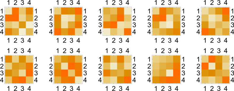
Figure 2: (color) Density plots of the original $(D,\,N)=(10,\,4)$ approximate numerical solution $\text{Abs}\big{[}\widehat{a}^{\,\mu}_{\kappa\text{-num-\text@underline{sol}-HERM}}\big{]}$ with $f_{\text{penalty}}=39.882$. Shown are $\mu=1,\,\ldots\,,5$ on the top row and $\mu=6,\,\ldots\,,10$ on the bottom row.

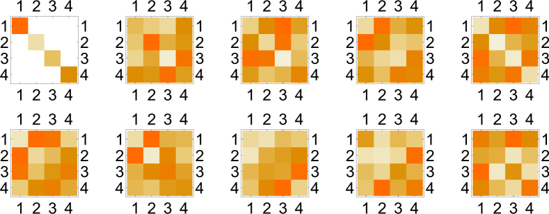
Figure 3: (color) Density plots of the transformed $(D,\,N)=(10,\,4)$ approximate numerical solution $\text{Abs}\big{[}\widehat{a}^{\;\prime\,\mu}_{\kappa\text{-num-\text@underline{sol}-HERM}}\big{]}$ with $f_{\text{penalty}}=39.882$. Shown are $\mu=1,\,\ldots\,,5$ on the top row and $\mu=6,\,\ldots\,,10$ on the bottom row.

Now, change the basis, in order to diagonalize and order the $\mu=1$ matrix. This gives the matrices

$$\widehat{a}^{\;\prime\,\mu}_{\kappa\text{-num-\text@underline{sol}-HERM}}\,,\;\;\;\text{for}\;\;\;\mu=1,\,\ldots\,,10\,.$$ (20)

Calculating the absolute values of the entries of these transformed matrices, there is not yet a clear signal for a diagonal/band-diagonal structure: see Fig. 3 and compare with Fig. 1 without dynamic fermions. Let us consider the result from Fig. 3 in somewhat more detail.

The first observation is that we can perhaps observe a trend if we look at the improving approximations as listed in the last five rows of Table 2. The five corresponding density plots of $\text{Abs}\big{[}\widehat{a}^{\;\prime\,\mu}_{\kappa\text{-num-\text@underline{sol}-HERM}}\big{]}$ are shown as Figs. 6–10 in Ref. [19]. In these figures, we can, for example, focus on the pattern of the $\mu=2$ matrix as it evolves with improving approximations (decreasing penalty function) and see that a very weak diagonal/band-diagonal structure appears at $f_{\text{penalty}}\sim 300$ and that this structure more or less stabilizes at lower values of $f_{\text{penalty}}$ (note that $N=4$ is still far away from infinity). The second observation is that, at best, we can expect to find only a mild diagonal/band-diagonal structure due to the dynamic-fermion effects, as was previously observed in the algebraic $(D,\,N)=(3,\,3)$ results [9].

Obviously, we would like to obtain an improved $(D,\,N)=(10,\,4)$ numerical solution with $f_{\text{penalty}}\lesssim 1$, but it is possible that the basic result as given in Fig. 3 does not change much. In any case, the $(D,\,N)=(10,\,4)$ numerical results shown here are, as mentioned in the last paragraph of Sec. 1, primarily intended to verify that the proposed method can be implemented. The actual $(D,\,N)=(10,\,4)$ results are only indicative and future work on supercomputers should go to larger values of $N$ (see Sec. 6 for further comments).

6 Discussion

A direct algebraic solution of the full bosonic master-field equation (1a) of the IIB matrix model cannot go much further than dimensionality $D=3$ and matrix size $N=3$. In the present paper, we have explored an indirect numerical approach. The qualification “indirect” indicates that the Pfaffian is not directly considered but rather its relative variation written as the trace term (15). With considerable effort, we have obtained an approximate numerical solution for the case $(D,\,N)=(10,\,4)$, which has a complex Pfaffian. Having a complex Pfaffian requires a conceptual reinterpretation of the bosonic master-field, with a Hermitian part possibly relevant to the emergence of spacetime and an anti-Hermitian part whose interpretation is unclear for the moment (perhaps this anti-Hermitian part is directly or indirectly relevant to the emergence of matter). Obviously, this is an important open question.

It is, however, difficult to go to $N$ values very much larger than 4, while keeping $D=10$. We now have a perhaps somewhat surprising suggestion, namely, to temporarily leave behind the purely algebraic equation and to return to the original Langevin differential equation, but with a special form of the noise matrices. Specifically, we suggest to use the quenched-master form for the Langevin noise matrices:

$$\eta^{\;\mu}_{\;kl}(\tau)=e^{\displaystyle{i\,\widehat{p}_{k}\,\tau}}\;\,\widehat{\eta}^{\;\mu}_{\;kl}\;\,e^{\displaystyle{-i\,\widehat{p}_{l}\,\tau}}\,,$$ (21)

with Langevin time $\tau$ and fixed random numbers $\widehat{p}_{k}$ and $\widehat{\eta}^{\;\mu}_{\;kl}$, where the matrix indices $k$ and $l$ take values from $\{1,\,2,\,\ldots\,,\,N\}$ and the directional index $\mu$ from $\{1,\,2,\,\ldots\,,\,D\}$. See Sec. 3.2 in Ref. [9] for a brief discussion of the characteristics of these random numbers $\widehat{p}_{k}$ and $\widehat{\eta}^{\;\mu}_{\;kl}$, the first having a uniform distribution and the second $D$ independent Gaussian distributions. See, furthermore, Sec. 2 of Ref. [2] for the proof that the noise (21) suffices in the large-$N$ limit (with planar diagrams dominating).

It appears that the $D=10$ setup and technology used in Ref. [12] [starting from Eqs. (3.2) and (3.3) in that reference], can be employed, but now with the special noise matrices (21). The idea is to extract, from the obtained numerical solution $\widehat{A}^{\;\mu}(\tau)$ at an equilibrium time $\tau_{\text{eq}}$, the constant master-field matrices $\widehat{a}^{\;\mu}$ by use of (9a), for the given values of $\widehat{p}_{k}$. The obtained matrices $\widehat{a}^{\;\mu}$ are expected to solve the algebraic equation (9b), at least within the numerical accuracy. Assuming that the trace term (15) can be evaluated accurately (with advanced numerical methods and powerful computers), it would seem that master-field matrices $\widehat{a}^{\;\mu}$ with sizes $N=64$ and $N=128$ could be within reach.

Appendix A Pfaffian for $D=10$ and $N\geq 2$

The fermion integration in the partition function of the $D=10$ IIB matrix model (2) with fermionic action (3) gives the Pfaffian (4) as a function of the bosonic matrices $A_{\mu}$. Explicitly, the Pfaffian evaluated for the master-field matrices $\widehat{a}_{\mu}$ reads [13, 14]

$$\mathcal{P}\left(\widehat{a}\,\right)\equiv\text{Pf}\left[\mathcal{M}\left(\widehat{a}\,\right)\right]\,,$$ (22a)

$$\mathcal{M}_{a\alpha\,,\,b\beta}=-i\,f_{abc}\,\big{(}\mathcal{C}\,\Sigma_{\mu}\big{)}_{\alpha\beta}\;\widehat{a}_{\mu}^{\;c}\,,$$ (22b)

with Lie-algebra indices $a,b,c$ running over $\{1,\,\ldots\,,\,(N^{2}-1)\}$, spinorial indices $\alpha,\beta$ running over $\{1,\,\ldots\,,\,16\}$, and the directional index $\mu$ being summed over $\{1,\,\ldots\,,\,10\}$, where the pair of indices $a\alpha$ gives a combined index $A$ and $b\beta$ gives a combined index $B$. For completeness, we give the definition of the Pfaffian in terms of the completely antisymmetric Levi–Civita symbol $\epsilon$ normalized to $1$. The Pfaffian of a $(2n)\times(2n)$ skew-symmetric matrix $A=(a_{ij})$ is then given by

$$\text{Pf}[A]\equiv\frac{1}{2^{n}\,n!}\;\epsilon_{i_{1}j_{1}i_{2}j_{2}\cdots i_{n}j_{n}}\;a_{i_{1}j_{1}}\,a_{i_{2}j_{2}}\cdots a_{i_{n}j_{n}}\,,$$ (23)

with implicit summations over repeated indices.

The real numbers $f_{abc}$ in (22b) are the structure constants from the $SU(N)$ traceless Hermitian generators $t_{a}$:

$$f_{abc}=-2\,i\,\text{Tr}\,\big{(}t_{a}\,\big{[}t_{b},\,t_{c}\big{]}\big{)}\,,$$ (24a)

$$\text{Tr}\,\big{(}t_{a}\cdot t_{b}\big{)}=\frac{1}{2}\;\delta_{ab}\,,$$ (24b)

where the last equation sets the normalization of the generators. The coefficients $\widehat{a}_{\mu}^{\;c}$ in (22b) have resulted from the expansion of the bosonic master-field matrix $\widehat{a}_{\mu}$ with respect to these generators,

$$\left(\widehat{a}_{\mu}\right)_{kl}=\widehat{a}_{\mu}^{\;c}\,\left(t_{c}\right)_{kl}\,.$$ (25)

The charge conjugation matrix $\mathcal{C}$ in (22b) becomes the unit matrix for an appropriate choice of $\Sigma_{\mu}$ matrices [14]:

$$\begin{array}[]{lll}&\Sigma_{1\phantom{0}}=\;i\,\sigma_{2}\otimes\sigma_{2}\otimes\sigma_{2}\otimes\sigma_{2}\,,&\Sigma_{2\phantom{0}}=\;i\,\sigma_{2}\otimes\sigma_{2}\otimes\makebox[2.58334pt][l]{$1$}{\rm l}\otimes\sigma_{1}\,,\\[5.69054pt] &\Sigma_{3\phantom{0}}=\;i\,\sigma_{2}\otimes\sigma_{2}\otimes\makebox[2.58334pt][l]{$1$}{\rm l}\otimes\sigma_{3}\,,&\Sigma_{4\phantom{0}}=\;i\,\sigma_{2}\otimes\sigma_{1}\otimes\sigma_{2}\otimes\makebox[2.58334pt][l]{$1$}{\rm l}\,,\\[5.69054pt] &\Sigma_{5\phantom{0}}=\;i\,\sigma_{2}\otimes\sigma_{3}\otimes\sigma_{2}\otimes\makebox[2.58334pt][l]{$1$}{\rm l}\,,&\Sigma_{6\phantom{0}}=\;i\,\sigma_{2}\otimes\makebox[2.58334pt][l]{$1$}{\rm l}\otimes\sigma_{1}\otimes\sigma_{2}\,,\\[5.69054pt] &\Sigma_{7\phantom{0}}=\;i\,\sigma_{2}\otimes\makebox[2.58334pt][l]{$1$}{\rm l}\otimes\sigma_{3}\otimes\sigma_{2}\,,&\Sigma_{8\phantom{0}}=\;i\,\sigma_{1}\otimes\makebox[2.58334pt][l]{$1$}{\rm l}\otimes\makebox[2.58334pt][l]{$1$}{\rm l}\otimes\makebox[2.58334pt][l]{$1$}{\rm l}\,,\\[5.69054pt] &\Sigma_{9\phantom{0}}=\;i\,\sigma_{3}\otimes\makebox[2.58334pt][l]{$1$}{\rm l}\otimes\makebox[2.58334pt][l]{$1$}{\rm l}\otimes\makebox[2.58334pt][l]{$1$}{\rm l}\,,&\Sigma_{10}=\;\makebox[2.58334pt][l]{$1$}{\rm l}\otimes\makebox[2.58334pt][l]{$1$}{\rm l}\otimes\makebox[2.58334pt][l]{$1$}{\rm l}\otimes\makebox[2.58334pt][l]{$1$}{\rm l}\;=\;\makebox[2.58334pt][l]{$1$}{\rm l}_{16}\,,\\ \end{array}$$ (26)

which are manifestly symmetric (so that the corresponding matrix $\mathcal{C}$ is trivial). Incidentally, we prefer to call these matrices “Sigma” by analogy to the 4-dimensional case with the four $4\times 4$ Dirac matrices $\gamma_{\mu}$ and the three $2\times 2$ Pauli matrices $\sigma_{a}$, to which $\sigma_{4}\equiv\makebox[2.58334pt][l]{$1$}{\rm l}$ is added.

The matrix dimension of $\mathcal{M}$ equals 48 for $N=2$, 128 for $N=3$, and 240 for $N=4$. With arbitrary numerical coefficients $\widehat{a}_{\mu}^{\;c}$, it can be readily verified that $\det[\mathcal{M}]=(\text{Pf}[\mathcal{M}])^{2}$ is positive and real for $N=2$ and $3$, but complex for $N=4$. This implies that the above Pfaffian is real for $N=2$ and $3$ and complex for $N=4$. The above Pfaffian is, in general, complex also for $N>4$ [14].

The homogeneous polynomial $\mathcal{P}\left(\widehat{a}\,\right)$ from (22a) has an order equal to half the dimension of $\mathcal{M}\left(\widehat{a}\,\right)$. Hence, the polynomial $\mathcal{P}\left(\widehat{a}\,\right)$ has order 24, 64, and 120 for $N=2$, $3$, and $4$, respectively. The corresponding algebraic equations (1a) are indeed huge.

Appendix B Pseudorandom numbers for $(D,\,N)=(10,\,4)$

In this appendix, we give the particular realization (the “$\kappa$-realization”) of the pseudorandom numbers used for the approximate numerical solution of Sec. 5.2 .

Specifically, we take the following 4 real pseudorandom numbers for the master momenta:

$$\widehat{p}_{\text{$\kappa$-realization}}=\left\{{-\frac{111}{250},\,\frac{19}{200},\,-\frac{63}{200},\,\frac{189}{1000}}\right\}\,,$$ (27)

and the following 150 real pseudorandom numbers entering the Hermitian master-noise matrices:

$$\widehat{\eta}^{\,1}_{\text{$\kappa$-realization}}=$$

$$\left(\!\!\begin{array}[]{cccc}\frac{593}{2000\sqrt{2}}-\frac{151}{500}&\frac{1}{2000}-\frac{9i}{40}&\frac{353}{2000}+\frac{6i}{25}&-\frac{987}{2000}-\frac{51i}{400}\\ \frac{1}{2000}+\frac{9i}{40}&\frac{151}{500}+\frac{593}{2000\sqrt{2}}&\frac{1}{8}-\frac{63i}{2000}&-\frac{131}{400}-\frac{367i}{2000}\\ \frac{353}{2000}-\frac{6i}{25}&\frac{1}{8}+\frac{63i}{2000}&-\frac{369}{1000}-\frac{593}{2000\sqrt{2}}&-\frac{169}{400}+\frac{171i}{500}\\ -\frac{987}{2000}+\frac{51i}{400}&-\frac{131}{400}+\frac{367i}{2000}&-\frac{169}{400}-\frac{171i}{500}&\frac{369}{1000}-\frac{593}{2000\sqrt{2}}\\ \end{array}\!\!\right)\!,$$ (28e)

$$\widehat{\eta}^{\,2}_{\text{$\kappa$-realization}}=$$

$$\left(\!\!\begin{array}[]{cccc}\frac{69}{2000}-\frac{17}{50\sqrt{2}}&-\frac{153}{500}-\frac{47i}{500}&\frac{897}{2000}-\frac{61i}{1000}&\frac{269}{2000}-\frac{237i}{2000}\\ -\frac{153}{500}+\frac{47i}{500}&-\frac{69}{2000}-\frac{17}{50\sqrt{2}}&\frac{1}{250}-\frac{13i}{200}&-\frac{103}{400}+\frac{367i}{1000}\\ \frac{897}{2000}+\frac{61i}{1000}&\frac{1}{250}+\frac{13i}{200}&\frac{17}{50\sqrt{2}}-\frac{123}{250}&\frac{1}{20}-\frac{71i}{2000}\\ \frac{269}{2000}+\frac{237i}{2000}&-\frac{103}{400}-\frac{367i}{1000}&\frac{1}{20}+\frac{71i}{2000}&\frac{123}{250}+\frac{17}{50\sqrt{2}}\\ \end{array}\!\!\right)\!,$$ (28j)

$$\widehat{\eta}^{\,3}_{\text{$\kappa$-realization}}=$$

$$\left(\!\!\begin{array}[]{cccc}\frac{313}{1000}+\frac{7}{250\sqrt{2}}&\frac{7}{200}+\frac{431i}{2000}&\frac{17}{40}-\frac{59i}{250}&-\frac{437}{2000}+\frac{69i}{1000}\\ \frac{7}{200}-\frac{431i}{2000}&\frac{7}{250\sqrt{2}}-\frac{313}{1000}&-\frac{991}{2000}-\frac{49i}{250}&\frac{83}{1000}-\frac{279i}{2000}\\ \frac{17}{40}+\frac{59i}{250}&-\frac{991}{2000}+\frac{49i}{250}&\frac{871}{2000}-\frac{7}{250\sqrt{2}}&\frac{49}{250}+\frac{121i}{500}\\ -\frac{437}{2000}-\frac{69i}{1000}&\frac{83}{1000}+\frac{279i}{2000}&\frac{49}{250}-\frac{121i}{500}&-\frac{871}{2000}-\frac{7}{250\sqrt{2}}\\ \end{array}\!\!\right)\!,$$ (28o)

$$\widehat{\eta}^{\,4}_{\text{$\kappa$-realization}}=$$

$$\left(\!\!\begin{array}[]{cccc}\frac{293}{1000}+\frac{429}{2000\sqrt{2}}&-\frac{11}{250}-\frac{469i}{2000}&-\frac{439}{1000}-\frac{483i}{2000}&-\frac{11}{50}+\frac{41i}{400}\\ -\frac{11}{250}+\frac{469i}{2000}&\frac{429}{2000\sqrt{2}}-\frac{293}{1000}&\frac{409}{1000}-\frac{343i}{2000}&\frac{3}{16}-\frac{407i}{1000}\\ -\frac{439}{1000}+\frac{483i}{2000}&\frac{409}{1000}+\frac{343i}{2000}&-\frac{6}{125}-\frac{429}{2000\sqrt{2}}&-\frac{141}{500}-\frac{31i}{2000}\\ -\frac{11}{50}-\frac{41i}{400}&\frac{3}{16}+\frac{407i}{1000}&-\frac{141}{500}+\frac{31i}{2000}&\frac{6}{125}-\frac{429}{2000\sqrt{2}}\\ \end{array}\!\!\right)\!,$$ (28t)

$$\widehat{\eta}^{\,5}_{\text{$\kappa$-realization}}=$$

$$\left(\!\!\begin{array}[]{cccc}\frac{183}{500\sqrt{2}}-\frac{48}{125}&\frac{37}{125}+\frac{249i}{1000}&-\frac{511}{2000}-\frac{43i}{500}&-\frac{129}{2000}+\frac{19i}{200}\\ \frac{37}{125}-\frac{249i}{1000}&\frac{48}{125}+\frac{183}{500\sqrt{2}}&\frac{49}{400}-\frac{463i}{1000}&\frac{23}{200}+\frac{433i}{2000}\\ -\frac{511}{2000}+\frac{43i}{500}&\frac{49}{400}+\frac{463i}{1000}&-\frac{46}{125}-\frac{183}{500\sqrt{2}}&\frac{821}{2000}+\frac{199i}{2000}\\ -\frac{129}{2000}-\frac{19i}{200}&\frac{23}{200}-\frac{433i}{2000}&\frac{821}{2000}-\frac{199i}{2000}&\frac{46}{125}-\frac{183}{500\sqrt{2}}\\ \end{array}\!\!\right)\!,$$ (28y)

$$\widehat{\eta}^{\,6}_{\text{$\kappa$-realization}}=$$

$$\left(\!\!\begin{array}[]{cccc}\frac{181}{1000}-\frac{181}{2000\sqrt{2}}&-\frac{143}{500}+\frac{i}{5}&\frac{921}{2000}-\frac{313i}{1000}&-\frac{603}{2000}-\frac{449i}{2000}\\ -\frac{143}{500}-\frac{i}{5}&-\frac{181}{1000}-\frac{181}{2000\sqrt{2}}&\frac{609}{2000}-\frac{39i}{2000}&\frac{443}{2000}+\frac{383i}{1000}\\ \frac{921}{2000}+\frac{313i}{1000}&\frac{609}{2000}+\frac{39i}{2000}&\frac{941}{2000}+\frac{181}{2000\sqrt{2}}&-\frac{17}{1000}+\frac{27i}{2000}\\ -\frac{603}{2000}+\frac{449i}{2000}&\frac{443}{2000}-\frac{383i}{1000}&-\frac{17}{1000}-\frac{27i}{2000}&\frac{181}{2000\sqrt{2}}-\frac{941}{2000}\\ \end{array}\!\!\right)\!,$$ (28ad)

$$\widehat{\eta}^{\,7}_{\text{$\kappa$-realization}}=$$

$$\left(\!\!\begin{array}[]{cccc}\frac{57}{2000}+\frac{83}{200\sqrt{2}}&-\frac{129}{500}-\frac{147i}{2000}&\frac{387}{2000}-\frac{611i}{2000}&\frac{313}{2000}+\frac{191i}{400}\\ -\frac{129}{500}+\frac{147i}{2000}&\frac{83}{200\sqrt{2}}-\frac{57}{2000}&-\frac{61}{500}-\frac{11i}{50}&-\frac{969}{2000}+\frac{927i}{2000}\\ \frac{387}{2000}+\frac{611i}{2000}&-\frac{61}{500}+\frac{11i}{50}&-\frac{2}{125}-\frac{83}{200\sqrt{2}}&\frac{489}{1000}+\frac{361i}{1000}\\ \frac{313}{2000}-\frac{191i}{400}&-\frac{969}{2000}-\frac{927i}{2000}&\frac{489}{1000}-\frac{361i}{1000}&\frac{2}{125}-\frac{83}{200\sqrt{2}}\\ \end{array}\!\!\right)\!,$$ (28ai)

$$\widehat{\eta}^{\,8}_{\text{$\kappa$-realization}}=$$

$$\left(\!\!\begin{array}[]{cccc}\frac{321}{2000}-\frac{193}{2000\sqrt{2}}&-\frac{273}{2000}-\frac{441i}{2000}&\frac{427}{1000}-\frac{317i}{2000}&-\frac{407}{2000}-\frac{57i}{400}\\ -\frac{273}{2000}+\frac{441i}{2000}&-\frac{321}{2000}-\frac{193}{2000\sqrt{2}}&\frac{23}{2000}+\frac{93i}{400}&\frac{163}{500}+\frac{18i}{125}\\ \frac{427}{1000}+\frac{317i}{2000}&\frac{23}{2000}-\frac{93i}{400}&\frac{307}{1000}+\frac{193}{2000\sqrt{2}}&\frac{333}{2000}-\frac{9i}{25}\\ -\frac{407}{2000}+\frac{57i}{400}&\frac{163}{500}-\frac{18i}{125}&\frac{333}{2000}+\frac{9i}{25}&\frac{193}{2000\sqrt{2}}-\frac{307}{1000}\\ \end{array}\!\!\right)\!,$$ (28an)

$$\widehat{\eta}^{\,9}_{\text{$\kappa$-realization}}=$$

$$\left(\!\!\begin{array}[]{cccc}-\frac{39}{400}-\frac{7}{200\sqrt{2}}&\frac{1}{500}-\frac{i}{125}&-\frac{981}{2000}+\frac{56i}{125}&-\frac{137}{1000}+\frac{547i}{2000}\\ \frac{1}{500}+\frac{i}{125}&\frac{39}{400}-\frac{7}{200\sqrt{2}}&-\frac{201}{1000}+\frac{101i}{1000}&-\frac{63}{500}+\frac{31i}{125}\\ -\frac{981}{2000}-\frac{56i}{125}&-\frac{201}{1000}-\frac{101i}{1000}&\frac{197}{400}+\frac{7}{200\sqrt{2}}&\frac{597}{2000}-\frac{57i}{125}\\ -\frac{137}{1000}-\frac{547i}{2000}&-\frac{63}{500}-\frac{31i}{125}&\frac{597}{2000}+\frac{57i}{125}&\frac{7}{200\sqrt{2}}-\frac{197}{400}\\ \end{array}\!\!\right)\!,$$ (28as)

$$\widehat{\eta}^{\,10}_{\text{$\kappa$-realization}}=$$

$$\left(\!\!\begin{array}[]{cccc}\frac{577}{2000\sqrt{2}}-\frac{319}{2000}&\frac{969}{2000}+\frac{2i}{5}&-\frac{243}{2000}+\frac{29i}{500}&-\frac{19}{125}-\frac{151i}{1000}\\ \frac{969}{2000}-\frac{2i}{5}&\frac{319}{2000}+\frac{577}{2000\sqrt{2}}&\frac{17}{50}+\frac{119i}{2000}&\frac{463}{2000}-\frac{33i}{400}\\ -\frac{243}{2000}-\frac{29i}{500}&\frac{17}{50}-\frac{119i}{2000}&\frac{119}{1000}-\frac{577}{2000\sqrt{2}}&\frac{257}{1000}+\frac{219i}{500}\\ -\frac{19}{125}+\frac{151i}{1000}&\frac{463}{2000}+\frac{33i}{400}&\frac{257}{1000}-\frac{219i}{500}&-\frac{119}{1000}-\frac{577}{2000\sqrt{2}}\\ \end{array}\!\!\right)\!.\vspace*{0mm}$$ (28ax)

Incidentally, the above matrices (28) also make clear what $4\times 4$ matrix realizations have been chosen for the $SU(4)$ generators $t_{a}$ from (24).

References

• [1] E. Witten, “The $1/N$ expansion in atomic and particle physics,” in G. ’t Hooft et. al (eds.), Recent Developments in Gauge Theories, Cargese 1979 (Plenum Press, New York, 1980).
• [2] J. Greensite and M.B. Halpern, “Quenched master fields,” Nucl. Phys. B 211, 343 (1983).
• [3] N. Ishibashi, H. Kawai, Y. Kitazawa, and A. Tsuchiya, “A large-$N$ reduced model as superstring,” Nucl. Phys. B 498, 467 (1997), arXiv:hep-th/9612115.
• [4] H. Aoki, S. Iso, H. Kawai, Y. Kitazawa, A. Tsuchiya, and T. Tada, “IIB matrix model,” Prog. Theor. Phys. Suppl.  134, 47 (1999), arXiv:hep-th/9908038.
• [5] F.R. Klinkhamer, “IIB matrix model: Emergent spacetime from the master field,” Prog. Theor. Exp. Phys. 2021, 013B04 (2021), arXiv:2007.08485.
• [6] F.R. Klinkhamer, “IIB matrix model and regularized big bang,” Prog. Theor. Exp. Phys. 2021, 063B05 (2021), arXiv:2009.06525.
• [7] F.R. Klinkhamer, “M-theory and the birth of the Universe,” Acta Phys. Pol. B 52, 1007 (2021), arXiv:2102.11202.
• [8] F.R. Klinkhamer, “A first look at the bosonic master-field equation of the IIB matrix model,” Int. J. Mod. Phys. D 30, 2150105 (2021) arXiv:2105.05831.
• [9] F.R. Klinkhamer, “Solutions of the bosonic master-field equation from a supersymmetric matrix model,” Acta Phys. Pol. B 52, 1339 (2021), arXiv:2106.07632.
• [10] S.W. Kim, J. Nishimura, and A. Tsuchiya, “Expanding (3+1)-dimensional universe from a Lorentzian matrix model for superstring theory in (9+1)-dimensions,” Phys. Rev. Lett.  108, 011601 (2012), arXiv:1108.1540.
• [11] J. Nishimura and A. Tsuchiya, “Complex Langevin analysis of the space-time structure in the Lorentzian type IIB matrix model,” JHEP 1906, 077 (2019), arXiv:1904.05919.
• [12] K.N. Anagnostopoulos, T. Azuma, Y. Ito, J. Nishimura, T. Okubo, and S. K. Papadoudis, “Complex Langevin analysis of the spontaneous breaking of 10D rotational symmetry in the Euclidean IKKT matrix model,” JHEP 2006, 069 (2020), arXiv:2002.07410.
• [13] W. Krauth, H. Nicolai, and M. Staudacher, “Monte Carlo approach to $M$-theory,” Phys. Lett. B 431, 31 (1998), arXiv:hep-th/9803117.
• [14] J. Nishimura and G. Vernizzi, “Spontaneous breakdown of Lorentz invariance in IIB matrix model,” JHEP 0004, 015 (2000), arXiv:hep-th/0003223.
• [15] J. Nishimura, private communication (2021).
• [16] S. Wolfram, Mathematica: A System for Doing Mathematics by Computer, Second Edition (Addison–Wesley, Redwood City CA, USA, 1991).
• [17] J.A. Nelder and R. Mead, “A simplex method for function minimization,” The Computer Journal, 7, 308 (1965); Errata ibid, 8, 27 (1965).
• [18] W.H. Press, S.A. Teukolsky, W.T. Vetterling, and B.P. Flannery, Numerical Recipes in FORTRAN: The Art of Scientific Computing (Cambridge University Press, Cambridge, UK, 1986).
• [19] F.R. Klinkhamer, “IIB matrix model, bosonic master field, and emergent spacetime,” talk at: Workshop on Quantum Geometry, Field Theory, and Gravity, Corfu Summer Institute, September 20–27, 2021 [slides available from https://www.itp.kit.edu/_media/research/corfu2021-klinkhamer-v4.
pdf].