Nucleon-nucleon interaction in chiral EFT with a finite cutoff: explicit perturbative renormalization at next-to-leading order

Abstract

We present a study of two-nucleon scattering in chiral effective field theory with a finite cutoff to next-to-leading order in the chiral expansion. In the proposed scheme, the contributions of the lowest-order interaction to the scattering amplitude are summed up to an arbitrary order, while the corrections beyond leading order are iterated only once. We consider a general form of the regulator for the leading-order potential including local and non-local structures. The main objective of the paper is to address formal aspects of renormalizability within the considered scheme. In particular, we provide a rigorous proof, valid to all orders in the iterations of the leading-order potential, that power-counting breaking terms originating from the integration regions with momenta of the order of the cutoff can be absorbed into the renormalization of the low energy constants of the leading contact interactions. We also demonstrate that the cutoff dependence of the scattering amplitude can be reduced by perturbatively subtracting the regulator artifacts at next-to-leading order. The obtained numerical results for phase shifts in $P$- and higher partial waves confirm the applicability of our scheme for nucleon-nucleon scattering.

I Introduction

Few-nucleon systems were first considered in the framework of chiral effective field theory by Weinberg in Refs. Weinberg (1990, 1991). For processes involving two and more nucleons, Weinberg suggested to apply the systematic power counting to the effective potential (instead of the amplitude as done for purely pionic or single-nucleon systems), which is defined as a sum of all $n$-nucleon-irreducible diagrams. To obtain the scattering amplitudes or other observables, one needs to solve the Lippmann-Schwinger or Schrödinger equation. Since then, there has been enormous progress in the realization of these ideas using, however, quite different approaches and philosophies. So far, there is no consensus in the community as to which approach is most efficient and suits best the principles of effective field theory. The descriptions of various schemes and methods can be found, e.g., in Refs. Ordonez and van Kolck (1992); Kaiser et al. (1997); Park et al. (1999); Gegelia (1998a); Birse et al. (1999); Birse (2006); Lutz (2000); Frederico et al. (1999); Higa and Robilotta (2003); Higa et al. (2004); Epelbaum et al. (1998, 2000); Kaplan et al. (1998a, b); Fleming et al. (2000); Beane et al. (2001, 2002); Kaiser (2001); Pavon Valderrama and Ruiz Arriola (2004, 2006); Nogga et al. (2005); Epelbaum and Meißner (2013); Djukanovic et al. (2007a); Long and van Kolck (2008); Yang et al. (2009); Valderrama (2011); Epelbaum and Gegelia (2009); Timoteo et al. (2011); Pavon Valderrama (2011); Albaladejo and Oller (2011); Long and Yang (2012); Epelbaum and Gegelia (2012); Gasparyan et al. (2013); Albaladejo and Oller (2012); Ren et al. (2018); Entem and Oller (2017); Behrendt et al. (2016); Pavón Valderrama et al. (2017); Reinert et al. (2018); Entem et al. (2017); Epelbaum et al. (2017, 2018); Kaplan (2020); Epelbaum et al. (2020a). For review articles and references see Refs. Bedaque and van Kolck (2002); Epelbaum et al. (2009); Machleidt and Entem (2011); Epelbaum and Meißner (2012); Epelbaum et al. (2020b); Hammer et al. (2020).

Chiral effective theory is an effective field theory (EFT) of QCD. It is based on the expansion of physical quantities around the chiral and zero-energy limits. The expansion parameter $Q$ is given by the ratio of the soft scale (pion mass $M_{\pi}$ and $3$-momenta of interacting particles $p$) denoted by $q$ and hard scale $\Lambda_{b}$: $Q=\frac{q}{\Lambda_{b}}$. The hard chiral symmetry breaking scale can be roughly identified with the mass of the lightest meson (excluding Goldstone bosons – pions), namely $\rho$-meson: $M_{\rho}\sim 770$ MeV. The main ingredient of chiral EFT is the most general effective Lagrangian containing pion and nucleon fields (we restrict ourselves to the case of two-flavor QCD) and consistent with symmetries of the underlying theory. It can be organized as a series of local terms with an increasing number of derivatives and/or powers of the quark mass insertions. Low-energy constants (LECs) accompanying the interaction terms in the effective Lagrangian account for effects of higher-energy physics.

In the purely pionic or single-nucleon sectors, the $S$-matrix is obtained from the effective Lagrangian by means of perturbation theory. In the two-nucleon case, a strictly perturbative expansion of the scattering amplitude is not applicable as otherwise the deuteron bound state could not be described. As argued by Weinberg Weinberg (1990, 1991), the reason for the failure of perturbation theory can be attributed to the enhancement of two-nucleon (2N) reducible diagrams by factors of $m_{N}/q$, where $m_{N}$ is the nucleon mass, as compared to the irreducible graphs with the same vertices and the number of loops. From the naive dimensional analysis, the leading contributions at order $Q^{0}$ are the one-pion exchange and non-derivative four-nucleon contact terms. The 2N-irreducible one-loop graphs with the leading-order (LO) vertices appear at the chiral order $Q^{2}$, whereas the 2N-reducible one-loop diagrams are of order $m_{N}Q^{2}/q=m_{N}q/\Lambda_{b}^{2}$. In few-nucleon applications, the latter factor is often counted as $\mathcal{O}(Q^{0})$ (i.e. $q/m_{N}\sim Q^{2}$), which is justified, in particular, by large numerical factors typically accompanying it. This means that all multiple iterations of the leading-order diagrams with intermediate two-nucleon states are of the same order and must be resummed in a non-perturbative manner. The contributions of higher-order terms in the chiral expansion can be formally treated perturbatively or non-perturbatively depending on the chosen scheme.

One should mention that within the so-called KSW approach Kaplan et al. (1996, 1998a, 1998b); Savage (1998), an attempt was made to resum only the iterations of the leading contact terms, whereas the iterations of the one-pion exchange were treated perturbatively. However, the convergence of such an approach is not satisfactory Gegelia (1998b, 1999a); Cohen and Hansen (1999); Fleming et al. (2000), which is a strong indication that also the leading-order one-pion exchange should be taken into account non-perturbatively if one aims at an efficient and convergent scheme. For a related recent work see Ref. Kaplan (2020).

The series of the resummed leading-order contributions (in particular, of the one-pion exchange) contains an infinite number of divergent terms with increasing power of divergence. Therefore, one needs to introduce an infinite number of counter terms in the effective Lagrangian in order to absorb them. In other words, the leading-order nucleon-nucleon amplitude defined this way is not renormalizable in the standard sense. A natural solution is to regularize this infinite series by introducing a regulator in the form of a cutoff.

Introducing a regulator requires special care. First of all, a regulator may break the symmetries (Lorentz, gauge, chiral) of the effective Lagrangian and, therefore, of the underlying theory. To avoid it, one can, in principle, introduce a regulator in the form that formally preserves all the symmetries using, e.g., the method of higher covariant derivatives Slavnov (1971), see Refs. Djukanovic et al. (2007b); Long and Mei (2016); Behrendt et al. (2016) for applications in the two-nucleon sector of chiral EFT. One should also keep in mind that the introduction of a cutoff may lead to regulator artifacts.

One proposed strategy of eliminating cutoff dependence and artifacts amounts to taking the cutoff much larger than the hard scale $\Lambda_{b}$ or even infinitely large, see e.g. Nogga et al. (2005). In such an approach, one has to introduce a contact term at leading order in each attractive spin-triplet partial wave where the one-pion-exchange contribution is regarded as non-perturbative in order to remove a strong cutoff dependence (and even more contact terms at higher orders Long and Yang (2012, 2011)). This scheme has been criticized in Epelbaum and Gegelia (2009); Epelbaum et al. (2018); Epelbaum et al. (2020a), in particular, because it does not provide an explicit transition to the regime with a perturbative one-pion exchange where one would need an infinite number of counter terms to absorb all divergent terms in the amplitude if the cutoff is infinite, or to remove the terms proportional to positive powers of $\Lambda$ if the cutoff is finite. Moreover, in such an approach, in attractive spin-triplet channels, a large (or infinite) number of spurious bound states is generated, which is at odds with the spectrum of the underlying theory. Therefore, we will not consider this scheme in the present work.

An alternative way is to set the cutoff value of the order of or smaller than the hard scale. In what follows, we will use a term “finite cutoff” assuming this prescription. The advantage of the choice of a cutoff to be of order $\Lambda_{b}$ Lepage (1997); Gegelia (1999b); Gegelia and Scherer (2006); Epelbaum and Meißner (2013) is that all positive powers of $\Lambda$ appearing in the iterations of the leading order potential are compensated by $\Lambda_{b}$ in the form $(\Lambda/\Lambda_{b})^{n}$ and do not blow up. The drawback of the “small” cutoff is that it distorts the analytic structure of the amplitude and there is a rather narrow window for its acceptable values if one wants to avoid artifacts. In this work, we propose a scheme where the effect of the regulator is systematically removed order by order in perturbation theory, so that smaller values of the cutoff can be used.

In calculations beyond leading order, a finite cutoff generates contributions that violate power counting. This is caused by the fact that typical integrals converge at momenta $p\sim\Lambda$ so that the terms such as $p^{2}/\Lambda_{b}^{2}$ become of order $\sim\Lambda^{2}/\Lambda_{b}^{2}\sim Q^{0}$ instead of $Q^{2}$. Usually, when working with a finite cutoff, one iterates subleading contributions by solving the Lippmann-Schwinger or Schrödinger equation (see Refs. Reinert et al. (2018); Entem et al. (2017); Reinert et al. (2021) for the most recent high-accuracy-level implementations) and assumes that power-counting breaking terms can be absorbed by renormalizing the relevant contact interactions. The renormalization is performed implicitly by adjusting the strength of the contact terms numerically. However, it is important to show whether such a renormalization can be realized explicitly and the power counting is indeed restored, so that the observed good agreement with experimental data is not accidental given the large number of adjustable parameters. It is also important to understand under which conditions the renormalization is possible. Such an understanding is necessary, in particular, if one aims at extending the calculations beyond the two-nucleon system, e.g. to few-nucleon dynamics and/or few-nucleon processes involving electroweak probes.

The usual requirement for a theory to be renormalizable is a possibility to absorb all ultraviolet divergences appearing in the $S$-matrix into a redefinition (renormalization) of the parameters of the effective Lagrangian without modifying its structure, i.e. respecting all symmetries of the theory. Obviously, introducing a finite cutoff automatically removes all ultraviolet divergences from the scattering amplitude. Nevertheless, as stated above, the problem is shifted to the appearance of positive powers of the cutoff in places where the power counting implies positive powers of the soft scale. Therefore, it is natural to extend the notion of renormalizability for the case at hand by requiring that all above mentioned power-counting breaking terms are absorbable by shifts (renormalization) of the low-energy constants of lower orders.

In this paper, we address the issue of the renormalizability in the above sense at next-to-leading (NLO) chiral order, i.e. $\mathcal{O}(Q^{2})$. We prove the renormalizability to all orders in the leading-order interaction $V_{0}$ by means of the Bogoliubov-Parasiuk-Hepp-Zimmermann (BPHZ) Bogoliubov and Parasiuk (1957); Hepp (1966); Zimmermann (1969) subtraction procedure in the $S$-waves. In higher partial waves, the renormalization at the considered chiral order works automatically. This result is useful in those channels where the series in $V_{0}$ converges (albeit possibly much slower than the chiral expansion). We allow for a rather general form of the regulator for $V_{0}$, including both local and non-local ones. Moreover, we also allow for the inclusion into the leading order interaction of contact terms quadratic in momenta in addition to the one-pion-exchange potential and derivativeless contact interactions. This feature may be particularly useful for approaches relying on a perturbative inclusion of higher-order corrections, where the unitarity of the scattering amplitude is maintained only approximately.

It should be emphasized that providing the renormalizability of the amplitude to all orders in $V_{0}$ does not necessarily imply the renormalizability in the non-perturbative regime, where the series in $V_{0}$ does not converge. This means that our results are not directly applicable in the channels that feature strong non-perturbative effects, or where the perturbative expansion is not expected to be efficient. In particular, this happens in ${}^{1}S_{0}$, ${}^{3}S_{1}-{{}^{3}D}_{1}$ and ${}^{3}P_{0}$ partial waves. Nevertheless, such a perturbative treatment is very instructive also in understanding the non-perturbative case and will serve as a crucial ingredient in our analysis of the non-perturbative renormalization in a subsequent publication.

Our paper is organized as follows. In Sec. II, we describe our formalism based on the effective Lagrangian, introduce the effective potential and discuss the calculation of the scattering amplitude. In Sec. III we demonstrate the validity of the power counting for the LO and NLO interactions in higher partial waves. The case of the $S$-waves and the problem of renormalization and the power-counting restoration is addressed separately in Sec. IV. The illustration of our formal findings for the case of the realistic nucleon-nucleon interaction is presented in Sec. V. The paper ends with a summary of the main findings. Useful bounds on the effective potential and their derivation are collected in Appendix.

II Formalism

II.1 Effective Lagrangian and power counting

An effective field theory is based on the most general effective Lagrangian consistent with the symmetries of the underlying theory Weinberg (1979). In chiral EFT, the relevant Lagrangian can be written as the sum of the pure pionic terms, the single nucleon terms, the two-nucleon interactions, etc.:

$$\mathcal{L}_{\rm eff}=\mathcal{L}_{\pi}^{(2)}+\mathcal{L}_{\pi}^{(4)}+\mathcal{L}_{\pi N}^{(1)}+\mathcal{L}_{\pi N}^{(2)}+\mathcal{L}_{NN}^{(0)}+\mathcal{L}_{NN}^{(2)}+\dots\,,$$ (1)

where the superscripts refer to the chiral order, i.e. to the number of derivatives and/or insertions of the pion mass. The explicit form of the terms in the effective Lagrangian can be found in Ref. Gasser and Leutwyler (1984) (for the pionic part), in Ref. Fettes et al. (2000) (for the pion-nucleon part) and in Ref. Girlanda et al. (2010) (for the nucleon-nucleon part). For the present study, the detailed structure of the Lagrangian and its particular realization is irrelevant.

The Lagrangian can be split into the (renormalized) kinetic and interaction terms:

$$\mathcal{L}_{\rm eff}(x) =: \mathcal{L}_{\text{kin}}^{N}(x)+\mathcal{L}_{\text{kin}}^{\pi}(x)+\mathcal{L}_{\text{int}}(x)\,,$$

$$\mathcal{L}_{\text{kin}}^{N}(x) = N^{\dagger}(x)\Big{(}i\partial_{0}+\frac{\vec{\nabla}^{2}}{2m_{N}}\Big{)}N(x)\,,\quad\mathcal{L}_{\text{kin}}^{\pi}(x)=\frac{1}{2}\partial_{\mu}{\bm{\pi}}(x)\cdot\partial^{\mu}{\bm{\pi}}(x)-{\frac{1}{2}}M_{\pi}^{2}\,{\bm{\pi}}(x)^{2},$$ (2)

where $N(x)$ is the large component of the nucleon field (we use the non-relativistic form of the Lagrangian) and ${\bm{\pi}}(x)$ is the pion field.

For estimating various contributions to the nucleon-nucleon scattering amplitude we adopt the standard Weinberg’s power counting Weinberg (1991) as a starting point. However, to be more general, we do not exclude possible promotions of formally higher-order contributions to lower orders. In Weinberg’s power counting, the chiral order for a potential contribution, i.e. the one corresponding to two-nucleon-irreducible diagrams (or more precisely to diagrams that do not possess the two-nucleon unitarity cut) is given by

$$D=2L+\sum_{i}\left(d_{i}+\frac{n_{i}}{2}-2\right)\,,$$ (3)

where $L$ is the number of loops, the sum runs over all vertices of the diagram, $n_{i}$ is the number of nucleon lines in vertex $i$ and $d_{i}$ is the number of derivatives and the pion-mass insertions at vertex $i$.

For the 2N-reducible amplitude with the potential components $\mathcal{V}^{(D_{1})}$, $\mathcal{V}^{(D_{2})}$,…,$\mathcal{V}^{(D_{k})}$ of orders $D_{1}$, $D_{2}$,…,$D_{k}$,

$$\mathcal{V}^{(D_{1})}\mathcal{G}\mathcal{V}^{(D_{2})}\mathcal{G}\dots\mathcal{G}\mathcal{V}^{(D_{k})}\equiv\int\left[\prod_{i=1}^{k-1}\frac{d^{4}p_{i}}{(2\pi)^{4}}\mathcal{G}(p_{i}^{\alpha_{i}},P^{\rho})\right]\mathcal{V}^{(D_{1})}(p^{\prime\nu},p_{1}^{\alpha_{1}})\mathcal{V}^{(D_{2})}(p_{1}^{\alpha_{1}},p_{2}^{\alpha_{2}})\dots\mathcal{V}^{(D_{k})}(p_{k-1}^{\alpha_{k-1}},p^{\mu})\,,$$ (4)

where, $P^{\rho}$ is the total $4$-momentum of the two-nucleon system and $p^{\mu}$, $p^{\prime\nu}$, $p_{i}^{\alpha_{i}}$ are the $4$-momenta of the first nucleon in the initial, final and intermediate state, respectively, the chiral order is given by the sum

$$D=D_{1}+D_{2}+\dots+D_{k}\,.$$ (5)

This enhancement is due to the infrared (pinch) singularity of the two-nucleon propagators $\mathcal{G}(p_{i},P)$ Weinberg (1991) appearing when both nucleons are on shell. Therefore, the leading-order potential $\mathcal{V}^{(0)}$ has to be iterated to an infinite order,

$$\mathcal{V}^{(0)}+\mathcal{V}^{(0)}\mathcal{G}\mathcal{V}^{(0)}+\mathcal{V}^{(0)}\mathcal{G}\mathcal{V}^{(0)}\mathcal{G}\mathcal{V}^{(0)}+\dots\,,$$ (6)

whereas the subleading-order potentials can be treated perturbatively. This is the scheme that we adopt in the present work.

Typically, the non-perturbative resummation of the potential contributions is performed using static (i.e. independent of the zeroth components of the momenta) potentials. Moreover, because of an infinite number of divergent diagrams appearing in the course of such a resummation, a regulator has to be introduced.

In order to include the regularized static potential contribution on the level of the Lagrangian, we add and subtract the non-local potential part to $\mathcal{L}_{\text{int}}$

$$\mathcal{L}_{\text{int}}=\mathcal{L}_{V}+\left(\mathcal{L_{\text{int}}}-\mathcal{L}_{V}\right)\,,$$ (7)

with

$$\mathcal{L}_{V}(x) =-\int d\vec{y}\,d\vec{y}\,^{\prime}\frac{1}{2}N^{\dagger}_{j_{1}}(x_{0},\vec{x}-\vec{y}\,^{\prime}/2)N^{\dagger}_{j_{2}}(x_{0},\vec{x}+\vec{y}\,^{\prime}/2)V(\vec{y}\,^{\prime},\vec{y})_{j_{1},j_{2};i_{1},i_{2}}N_{i_{2}}(x_{0},\vec{x}+\vec{y}/2)N_{i_{1}}(x_{0},\vec{x}-\vec{y}/2)\,,$$ (8)

where $i_{1},i_{2},j_{1},j_{2}$ are the combined spin and isospin indices of the corresponding nucleons. The potential function $V(\vec{x}\,^{\prime},\vec{x})$ is the Fourier transform of the center-of-mass (c.m.) plane-wave potential $V(\vec{p}\,^{\prime},\vec{p})$:

$$V(\vec{x}\,^{\prime},\vec{x})=\int\frac{d^{3}p}{(2\pi)^{3}}\frac{d^{3}p^{\prime}}{(2\pi)^{3}}V(\vec{p}\,^{\prime},\vec{p})e^{i\vec{p}\cdot\vec{x}}e^{-i\vec{p}\,^{\prime}\cdot\vec{x}\,^{\prime}}\,,$$ (9)

where $\vec{p}$ ($\vec{p}\,^{\prime}$) is the c.m. momentum of the initial (final) nucleon. The case of a local potential corresponds to

$$V(\vec{p}\,^{\prime},\vec{p})=V(\vec{q}=\vec{p}\,^{\prime}-\vec{p})\,,\quad V(\vec{x}\,^{\prime},\vec{x})=V(\vec{x})\delta(\vec{x}\,^{\prime}-\vec{x})\,.$$ (10)

The potential $V$ can be regularized using various types of regulators: local, non-local, semilocal or even a lattice regularization.

Now, we can organize the potential in accordance with the chiral expansion:

$$V=V^{(0)}+V^{(2)}+V^{(3)}+V^{(4)}+\dots$$ (11)

Bare potentials $V^{(i)}$ can be split into the renormalized parts $V_{i}$ and the counter terms $\delta V_{i}$:

$$V^{(i)}=V_{i}+\delta V_{i}\,,\quad\delta V_{i}=\delta V_{i}^{(2)}+\delta V_{i}^{(3)}+\delta V_{i}^{(4)}+\dots$$ (12)

The counter terms $\delta V_{i}^{(j)}$ ($j>i$) absorb the power counting violating terms appearing at order $\mathcal{O}(Q^{j})$. They have the form of polynomials in momenta (of the same power as present in $V_{i}$) and are either unregulated or regulated with an arbitrarily large cutoff in order to make all integrals well defined.

One can easily iterate the renormalized leading order potential $V_{0}$ performing the integrations over the zeroth components of the intermediate momenta (we suppress the spin and isospin indices):

$$V_{0}\sum_{n=0}^{\infty}\left(\mathcal{G}V_{0}\right)^{n}=V_{0}\sum_{n=0}^{\infty}\left(GV_{0}\right)^{n}=V_{0}(\vec{p}\,^{\prime},\vec{p})+\sum_{n=1}^{\infty}\int\bigg{[}\prod_{i=1}^{n}\frac{d^{3}p_{i}}{(2\pi)^{3}}G(p_{i};p_{\text{on}})\bigg{]}V_{0}(\vec{p}\,^{\prime},\vec{p}_{1})\dots V_{0}(\vec{p}_{n},\vec{p})\,,$$ (13)

since the potential $V_{0}$ is static. The two-nucleon propagator $G$ is given by

$$G(p_{i};p_{\text{on}})=\frac{m_{N}}{p_{\text{on}}^{2}-p_{i}^{2}+i\epsilon}\,,$$ (14)

where $p_{i}$ and $p_{\text{on}}$ are the absolute values of the intermediate and on-shell $3$-momenta, respectively.

The potential terms $V^{(i)}$ correspond to the two-nucleon-irreducible contributions $\mathcal{V}^{(i)}$ to the scattering amplitude constructed from the original Lagrangian $\mathcal{L}_{\text{int}}$ so that we can write

$$\mathcal{V}^{(i)}=V^{(i)}+\delta\mathcal{V}^{(i)}\,.$$ (15)

The difference $\delta\mathcal{V}^{(i)}$ can originate from the regulator corrections (the difference of the regulated and unregulated potential, see below), from explicit $1/m_{N}$ corrections and from the non-static contributions:

$$\delta\mathcal{V}^{(i)}=\delta_{\Lambda}V^{(i)}+\delta_{1/m_{N}}V^{(i)}+\delta_{\text{n.s.}}V^{(i)}\,.$$ (16)

The non-static corrections are defined to vanish on-shell ($p_{0}=\vec{p}\,^{2}/(2m_{N})$); thus, they cancel the pinch singularities in the nucleon propagators and contribute to higher orders due to the absence of the infrared enhancement. Therefore, all corrections contained in $\left(\mathcal{L_{\text{int}}}-\mathcal{L}_{V}\right)$ can be treated perturbatively. Note that the counter terms $\delta V_{i}^{(j)}$ do not contribute to $\delta\mathcal{V}^{(i)}$ because they are static (or can be chosen to be static using equations of motion) and unregulated.

In fact, non-potential contributions stemming from $\left(\mathcal{L_{\text{int}}}-\mathcal{L}_{V}\right)$, i.e. the ones that cannot be cast into the form of the static $NN$ potential as in Eq. (8), can be eliminated from the nucleon-nucleon scattering amplitude at low energies. This can be shown, e.g., by the method of unitary transformations Epelbaum et al. (1998, 2000) or applying time-ordered perturbation theory Pastore et al. (2009). Notice also a close connection of the considered matching to the methods of the potential non-relativistic QED and QCD Caswell and Lepage (1986); Pineda and Soto (1998, 1999); Brambilla et al. (2000, 2005). As long as we stay well below the pion production threshold, all effects of radiation pions can be reduced to the contact interactions with a non-analytic $M_{\pi}$ dependence Mehen and Stewart (2000); Mondejar and Soto (2007). In this work, we do not focus on the $M_{\pi}$ dependence of the nucleon-nucleon amplitude and can, therefore, ignore the $M_{\pi}$ dependence of the parameters in the effective Lagrangian.

For illustration, we show how the non-static corrections to the one-pion-exchange potential

$$\delta_{\text{n.s.}}\mathcal{V}^{(0)}_{1\pi}=\mathcal{V}^{(0)}_{1\pi}-V^{(0)}_{1\pi}=\mathcal{V}^{(0)}_{1\pi}-\mathcal{V}^{(0)}_{1\pi}\Big{|}_{p_{0}=p^{\prime}_{0}=\frac{p_{\text{on}}^{2}}{2m_{N}}}\,,$$ (17)

where we have ignored, for simplicity, all other corrections ($1/\Lambda$, $1/m_{N}$), are combined into various potential terms of higher orders. The non-static corrections start to appear at next-to-leading order, i.e. at order $\mathcal{O}(Q^{2})$:

$$T_{\text{n.s.}}^{(2)}=\sum_{m,n=0}^{\infty}(V^{(0)}_{1\pi}\mathcal{G})^{m}\left(\delta_{\text{n.s.}}\mathcal{V}^{(0)}_{1\pi}+\delta_{\text{n.s.}}\mathcal{V}^{(0)}_{1\pi}\mathcal{G}\,\delta_{\text{n.s.}}\mathcal{V}^{(0)}_{1\pi}\right)(\mathcal{G}V^{(0)}_{1\pi})^{n}\,.$$ (18)

The term quadratic in $\delta_{\text{n.s.}}\mathcal{V}^{(0)}_{1\pi}$ in Eq. (18) is also of order $\mathcal{O}(Q^{2})$ because there are terms where both factors $\delta_{\text{n.s.}}\mathcal{V}^{(0)}_{1\pi}$ cancel the pinch singularity in the same propagator $\mathcal{G}$. Therefore, it is convenient to rearrange the corrections due to $\delta_{\text{n.s.}}\mathcal{V}^{(0)}_{1\pi}$ in the following way. Summing all orders in $\delta_{\text{n.s.}}\mathcal{V}^{(0)}_{1\pi}$, we first obtain the exact formal expression for the non-static amplitude:

$$T_{\text{n.s.}}=\mathcal{V}^{(0)}_{1\pi}\frac{1}{1-\mathcal{G}\mathcal{V}^{(0)}_{1\pi}}=\left(V^{(0)}_{1\pi}+\delta_{\text{n.s.}}\mathcal{V}^{(0)}_{1\pi}\right)\frac{1}{1-\mathcal{G}\left(V^{(0)}_{1\pi}+\delta_{\text{n.s.}}\mathcal{V}^{(0)}_{1\pi}\right)}\,.$$ (19)

For the on-shell amplitude, we get the fully static approximation also if instead of replacing $\mathcal{V}^{(0)}_{1\pi}$ with $V^{(0)}_{1\pi}$, we replace $\mathcal{G}$ with

$$\hat{G}(p^{\mu},P^{\nu})=G(p;p_{\text{on}})2\pi\delta\left(p_{0}-\frac{\vec{p}\,^{2}}{2m_{N}}\right)\,.$$ (20)

The on-shell static amplitude is then given by

$$T_{\text{st}}=V^{(0)}_{1\pi}\frac{1}{1-\mathcal{G}V^{(0)}_{1\pi}}=\mathcal{V}^{(0)}_{1\pi}\frac{1}{1-\hat{G}\mathcal{V}^{(0)}_{1\pi}}\,.$$ (21)

This equivalence is an obvious consequence of the fact that integrals over the zeroth component can be easily performed when the integrand involves only static potentials. Expanding Eq. (19) in $\delta G=\mathcal{G}-\hat{G}$, we obtain:

$$T_{\text{n.s.}} = \mathcal{V}^{(0)}_{1\pi}\left\{\left[1-\delta\mathcal{G}\mathcal{V}^{(0)}_{1\pi}\left(1-\hat{G}\mathcal{V}^{(0)}_{1\pi}\right)^{-1}\right]\left(1-\hat{G}\mathcal{V}^{(0)}_{1\pi}\right)\right\}^{-1}$$ (22)

$$= \mathcal{V}^{(0)}_{1\pi}\left(1-\hat{G}\mathcal{V}^{(0)}_{1\pi}\right)^{-1}\sum_{n=0}^{\infty}\left[\delta\mathcal{G}\mathcal{V}^{(0)}_{1\pi}\left(1-\hat{G}\mathcal{V}^{(0)}_{1\pi}\right)^{-1}\right]^{n}$$

$$= T_{\text{st}}+\left(1-V^{(0)}_{1\pi}\hat{G}\right)^{-1}\mathcal{V}^{(0)}_{1\pi}\delta\mathcal{G}\mathcal{V}^{(0)}_{1\pi}\left(1-\hat{G}V^{(0)}_{1\pi}\right)^{-1}+\left(1-V^{(0)}_{1\pi}\hat{G}\right)^{-1}\mathcal{V}^{(0)}_{1\pi}\delta\mathcal{G}\mathcal{V}^{(0)}_{1\pi}\delta\mathcal{G}\mathcal{V}^{(0)}_{1\pi}\left(1-\hat{G}V^{(0)}_{1\pi}\right)^{-1}$$

$${}+\left(1-V^{(0)}_{1\pi}\hat{G}\right)^{-1}\mathcal{V}^{(0)}_{1\pi}\delta\mathcal{G}\mathcal{V}^{(0)}_{1\pi}\hat{G}\left(1-V^{(0)}_{1\pi}\hat{G}\right)^{-1}\mathcal{V}^{(0)}_{1\pi}\delta\mathcal{G}\mathcal{V}^{(0)}_{1\pi}\left(1-\hat{G}V^{(0)}_{1\pi}\right)^{-1}+\dots$$

$$= T_{\text{st}}+\sum_{m,n=0}^{\infty}\left(V^{(0)}_{1\pi}G\right)^{m}\left(V_{2\pi}^{(2)}+V_{3\pi}^{(4)}+\dots\right)\left(GV^{(0)}_{1\pi}\right)^{n}+\sum_{m,n,k=0}^{\infty}\left(V^{(0)}_{1\pi}G\right)^{m}V_{2\pi}^{(2)}G\left(V^{(0)}_{1\pi}G\right)^{k}V_{2\pi}^{(2)}\left(GV^{(0)}_{1\pi}\right)^{n}$$

$${}+\dots\,,$$

where the quantities

$$V_{2\pi}^{(2)}=\mathcal{V}^{(0)}_{1\pi}\delta\mathcal{G}\mathcal{V}^{(0)}_{1\pi}\Big{|}_{p_{0}=p^{\prime}_{0}=\frac{p_{\text{on}}^{2}}{2m_{N}}}\,,\quad V_{3\pi}^{(4)}=\mathcal{V}^{(0)}_{1\pi}\delta\mathcal{G}\mathcal{V}^{(0)}_{1\pi}\delta\mathcal{G}\mathcal{V}^{(0)}_{1\pi}\Big{|}_{p_{0}=p^{\prime}_{0}=\frac{p_{\text{on}}^{2}}{2m_{N}}}$$ (23)

can be identified (up to $1/m_{N}$-terms) with the static potentials corresponding to the $2\pi$- and $3\pi$-exchange box diagrams.

One should emphasize that the leading-order potential $V^{(0)}$ (or, more precisely, the corresponding term in the Lagrangian) is iterated only in two-nucleon reducible diagrams, whose contributions are enhanced. When there is no infrared enhancement, $V^{(0)}$ needs not be iterated. Moreover, in such a case, $V^{(0)}$ is not enhanced with respect to $\delta\mathcal{V}^{(0)}$. Therefore, one has to take into account the whole contribution $V^{(0)}+\delta\mathcal{V}^{(0)}=\mathcal{V}^{(0)}$. Consider, e.g., diagram $(a)$ in Fig. 1 with the insertion of the static one-pion exchange potential $V^{(0)}_{1\pi}$, which is not enhanced. Notice that the somewhat unusual type of diagrams in the left-hand side of the depicted equation reflects the appearance of the nonlocal “vertex” $\mathcal{L}_{V}$ in the Lagrangian $\mathcal{L}_{\rm int}$. The diagram $(b)$ with the insertion of $\delta\mathcal{V}^{(0)}_{1\pi}$ is of the same order and has to be included on the same footing. The sum of diagrams $(a)$ and $(b)$ results in diagram $(c)$, which is a regular $2\pi$-exchange crossed box diagram.

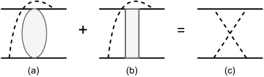
Figure 1: An example of a diagram with the insertion of ${V}^{(0)}_{1\pi}$ (denoted by the ellipse) without an infrared enhancement and the same diagram with the insertion of $\delta\mathcal{V}^{(0)}_{1\pi}$ (denoted by the rectangle). Dashed and solid lines refer to pions and nucleons, respectively. The sum of these diagrams is the crossed box two-pion-exchange diagram.

Eventually, the part of the effective Lagrangian that is relevant for nucleon-nucleon amplitude is given by

$$\mathcal{L}(x)=\mathcal{L}_{\text{kin}}^{N}(x)+\mathcal{L}_{V}(x)+\mathcal{L}_{\delta_{\Lambda}V}(x)\,,$$ (24)

where $\mathcal{L}_{\delta_{\Lambda}V}(x)$ is the part corresponding to the potential $\delta_{\Lambda}V$, which represents the correction due to a finite cutoff:

$$\delta_{\Lambda}V=\sum_{i}\delta_{\Lambda}V^{(i)}\,,\quad\delta_{\Lambda}V^{(i)}:=V^{(i)}_{\Lambda=\infty}-V^{(i)}_{\Lambda}\,.$$ (25)

In $V^{(i)}_{\Lambda=\infty}$, one can set $\Lambda$ to be arbitrarily large but finite to make integrals mathematically well-defined. If one keeps the $\delta_{\Lambda}V$ term in the Lagrangian, the whole Lagrangian remains formally independent of both the form of the regulator and the cutoff value. Of course, the nucleon-nucleon amplitude calculated at any finite order in chiral EFT does not feature this property. This is caused by the fact that only the leading order potential is iterated in a (possibly) non-perturbative manner, whereas the subleading contributions are treated perturbatively. Different choices of the regulator can lead to different non-perturbative regimes as reflected by a different number of (quasi)bound states, etc.. Perturbative corrections at higher orders can obviously not change such a regime. Therefore, one should choose the regulator such that the non-perturbative regime matches empirical observations. In particular, large values of the cutoff for the leading-order potential as considered e.g. in Ref. Nogga et al. (2005) are excluded in our scheme since they would lead to the appearance of spurious bound states in attractive spin-triplet channels. For low partial waves, this typically happens for cutoffs $\Lambda\gtrsim\Lambda_{b}$.

Nevertheless, taking into account the $\delta_{\Lambda}V$ terms will supposedly make the remaining cutoff dependence within the chosen non-perturbative regime weaker. In particular, if the leading-order potential is local and of Yukawa type, the left-hand singularities originating from the regulator are always perturbative Martin (1961). Thus, they will be shifted further away from the physical region after each correction due to $\delta_{\Lambda}V$. We will study numerically the effect of including the $\delta_{\Lambda}V$ terms in connection with the cutoff dependence in Sec. V. A formal analysis of such contributions and its interplay with the renormalization of the Lagrangian parameters requires the treatment of terms in the amplitude higher than NLO, which is beyond the scope of this paper.

If one chooses the cutoff of order $\Lambda_{b}$, one can formally expand $\delta_{\Lambda}V$ in $1/\Lambda$ and absorb the expanded terms into the nucleon-nucleon contact interactions, although the symmetries of the original Lagrangian will, in general, be lost. Note that this cannot be done for a non-local regulator of the long-range part of the potential (such as the one-pion-exchange potential) because of the mixture of long-range and short-range contributions. Moreover, even in the cases when such an expansion is possible, it might turn out to be more efficient to keep $\delta_{\Lambda}V$ unexpanded if the expansion converges slowly. In particular, one may benefit from keeping the $\delta_{\Lambda}V$ term if the cutoff is chosen to be smaller than $\Lambda_{b}$. One can even perform the expansion of the amplitude in $\delta_{\Lambda}V$ independently from the chiral expansion in $1/\Lambda_{b}$. The possibility to go to smaller values of $\Lambda$ is a welcome feature, e.g., for many-body applications.

In the present study, we analyze the leading and next-to-leading order nucleon-nucleon amplitude $T_{0}$ and $T_{2}$ using the following notation:

$$T_{0}=\sum_{n=0}^{\infty}T_{0}^{[n]}\,,\quad T_{0}^{[n]}=V_{0}K^{n}\,,$$

$$T_{2}=\sum_{m,n=0}^{\infty}T_{2}^{[m,n]}\,,\quad T_{2}^{[m,n]}=\bar{K}^{m}V_{2}K^{n}\,,$$

$$K=GV_{0}\,,\quad\bar{K}=V_{0}G\,,\quad V_{0}=V^{(0)}\,,\quad V_{2}=V^{(2)}+\delta_{\Lambda}V_{0}\,,$$ (26)

where we consider $\delta_{\Lambda}V_{0}$ to be of the same order as $V^{(2)}$. The explicit expressions for $V_{0}$ and $V_{2}$ will be given in Secs. II.2, II.3.

We assume that the series for $T_{0}$ and $T_{2}$ in Eq. (26) converge even though one might need to take into account several terms in the expansion to obtain an accurate result. The truly non-perturbative treatment of the leading-order interaction based on the findings of the present work will be considered in a subsequent publication. The above convergence assumption implies that we should exclude from the numerical analysis the partial waves with strong non-perturbative effects, namely ${}^{1}S_{0}$, ${}^{3}S_{1}$ and ${}^{3}P_{0}$ (although the formal treatment is applicable to all partial waves).

Note that the analysis of the power counting in this section was so far based on formal arguments. Many contributions to the amplitude were claimed to be of a certain (high) order even though they are mathematically not well defined (i.e. divergent). Such a procedure can only be justified if one can prove that the renormalized amplitude, i.e. the one expressed in terms of the renormalized quantities, indeed obeys the formal power counting. One of the main objectives of our study is to prove that the amplitudes $T_{0}$ and $T_{2}$ defined in Eq. (26) obey the assumed power counting meaning that all power-counting breaking contributions in $T_{2}$ stemming from the integrations over large momenta can be absorbed into contact interactions. For $T_{2}$, the only counter terms of a lower order are the leading-order $S$-wave momentum-independent contact interactions. Therefore, in addition to $T_{2}$ defined in Eq. (26), there is a contribution from the counter terms $\delta V_{0}^{(2)}=\sum_{s,t=0}^{\infty}\delta V_{0}^{(2),[s,t]}$:

$$\delta T_{2}=\sum_{m,n=0}^{\infty}\delta T_{2}^{[m,n]}\,,\quad\delta T_{2}^{[m,n]}=\sum_{s=0}^{m}\sum_{t=0}^{n}\bar{K}^{m-s}\delta V_{0}^{(2),[s,t]}K^{n-t}\,.$$ (27)

The explicit form of the counter terms will be specified in Sec. IV, see Eqs. (86), (89).

II.2 Leading-order potential

The leading-order potential $V_{0}(\vec{p}\,^{\prime},\vec{p})$ that we consider is the sum of the regulated static one-pion-exchange potential and the short-range part:

$$V_{0}(\vec{p}\,^{\prime},\vec{p}\,)=V^{(0)}_{1\pi,\Lambda}(\vec{p}\,^{\prime},\vec{p})+V^{(0)}_{\text{short},\Lambda}(\vec{p}\,^{\prime},\vec{p})\,.$$ (28)

II.2.1 Short-range leading-order potential

As already pointed out in the introduction, the short-range part of the leading-order potential can be chosen to include the momentum-independent contact interactions $V_{C_{S}}$, $V_{C_{T}}$ and contact terms quadratic in momenta $V_{C_{1,\ldots,7}}$ multiplied by the power-like non-local form factor of an appropriate power $n$:

$$V^{(0)}_{\text{short},\Lambda}(\vec{p}\,^{\prime},\vec{p})=\sum_{i=S,T,1,..,7}C_{i}\,V_{C_{i}}\,F_{\Lambda_{i},n_{i}}(p\,^{\prime},p)\,,$$ (29)

with

$$F_{\Lambda,n}(p\,^{\prime},p)=F_{\Lambda,n}(p\,^{\prime})F_{\Lambda,n}(p)\,,\quad F_{\Lambda,n}(p)=\left[F_{\Lambda}(p)\right]^{n}\,,\quad F_{\Lambda}(p)=\frac{\Lambda^{2}}{p^{2}+\Lambda^{2}}\,.$$ (30)

One can also introduce a regulator of a Gaussian form by replacing $F_{\Lambda,n}(p)$ with

$$F_{\Lambda,\text{exp}}(p)=\exp{(-p^{2}/\Lambda^{2})}\,.$$ (31)

The explicit form of the contact interactions is given by Epelbaum et al. (2005)

$$\{V_{C_{S}},V_{C_{T}}\} = \{1\,,\;\vec{\sigma}_{1}\cdot\vec{\sigma}_{2}\}$$

$$\{V_{C_{1}},\ldots,V_{C_{7}}\} = \{q^{2}\,,\;k^{2}\,,\;q^{2}(\vec{\sigma}_{1}\cdot\vec{\sigma}_{2})\,,\;k^{2}(\vec{\sigma}_{1}\cdot\vec{\sigma}_{2})\,,\;\frac{i}{2}(\vec{\sigma}_{1}+\vec{\sigma}_{2})\cdot(\vec{k}\times\vec{q}\,)\,,\;(\vec{q}\cdot\vec{\sigma}_{1})(\vec{q}\cdot\vec{\sigma}_{2})\,,\;(\vec{k}\cdot\vec{\sigma}_{1})(\vec{k}\cdot\vec{\sigma}_{2})\}\,,$$ (32)

where $\vec{q}=\vec{p}\,^{\prime}-\vec{p}$ and $\vec{k}=(\vec{p}\,^{\prime}+\vec{p})/2$. The contact terms can be equivalently expressed in terms of the partial-wave projectors $P_{i}$, $i={{}^{1}S_{0}}$, ${}^{3}S_{1}$, ${}^{3}S_{1}\to{{}^{3}D_{1}}$, ${}^{1}P_{1}$, ${}^{3}P_{1}$, ${}^{3}P_{0}$, ${}^{3}P_{2}$ Epelbaum et al. (2005).

Alternatively, one could introduce local short-range interactions (for the terms that depend only on $\vec{q}$, except for the spin-orbit term) using a different basis Gezerlis et al. (2014)

$$V^{(0)}_{\text{short},\Lambda}(\vec{p}\,^{\prime},\vec{p}\,)=\sum_{i=S,T,1,..,7}\tilde{C}_{i}\,V_{\tilde{C}_{i}}\,F_{q,\Lambda_{i},n_{i}}(\vec{p}\,^{\prime},\vec{p})\,,$$ (33)

with

$$V_{\tilde{C}_{i}} = V_{C_{i}}\,,\quad\text{ for }\,i=S,T,1,3,5,6\,,$$

$$\{V_{\tilde{C}_{2}},\;V_{\tilde{C}_{4}},\;V_{\tilde{C}_{7}}\} = \{q^{2}\,{\bm{\tau}}_{1}\cdot{\bm{\tau}}_{2}\,,\;q^{2}(\vec{\sigma}_{1}\cdot\vec{\sigma}_{2})\,{\bm{\tau}}_{1}\cdot{\bm{\tau}}_{2}\,,\;(\vec{q}\cdot\vec{\sigma}_{1})(\vec{q}\cdot\vec{\sigma}_{2}){\bm{\tau}}_{1}\cdot{\bm{\tau}}_{2}\}$$ (34)

and the local regulator

$$F_{q,\Lambda,n}(\vec{p}\,^{\prime},\vec{p}\,)=[F_{\Lambda}(q)]^{n}=\left(\frac{\Lambda^{2}}{q^{2}+\Lambda^{2}}\right)^{n}\,,$$ (35)

or with the regulator in the Gaussian form $F_{\Lambda,\text{exp}}(q)$.

II.2.2 One-pion-exchange potential

We split the one-pion-exchange potential into the triplet, singlet, and contact parts

$$V^{(0)}_{1\pi}=-\bigg{(}\frac{g_{A}}{2F_{\pi}}\bigg{)}^{2}\bm{\tau}_{1}\cdot\bm{\tau}_{2}\,\frac{\vec{\sigma}_{1}\cdot\vec{q}\,\vec{\sigma}_{2}\cdot\vec{q}}{q^{2}+M_{\pi}^{2}}=:V^{(0)}_{1\pi,\text{t}}+V^{(0)}_{1\pi,\text{s}}+V^{(0)}_{1\pi,\text{ct}}\,,$$ (36)

with

$$V^{(0)}_{1\pi,\text{s}} = \bigg{(}\frac{g_{A}}{2F_{\pi}}\bigg{)}^{2}\bm{\tau}_{1}\cdot\bm{\tau}_{2}\,\frac{(\vec{\sigma}_{1}\cdot\vec{\sigma}_{2}-1)}{4}\frac{M_{\pi}^{2}}{q^{2}+M_{\pi}^{2}}\,,$$

$$V^{(0)}_{1\pi,\text{ct}} = -\bigg{(}\frac{g_{A}}{2F_{\pi}}\bigg{)}^{2}\bm{\tau}_{1}\cdot\bm{\tau}_{2}\,\frac{(\vec{\sigma}_{1}\cdot\vec{\sigma}_{2}-1)}{4}\,.$$ (37)

All three parts can be regularized separately. The contact part $V_{1\pi,\text{ct}}$ can be absorbed by the leading-order ${}^{1}S_{0}$ contact term and thus needs not be considered separately. The triplet and singlet potential can be regularized by means of the non-local form factor (see Eq. (30)):

$$V^{(0)}_{1\pi,\Lambda}(\vec{p}\,^{\prime},\vec{p}\,)=V^{(0)}_{1\pi,\text{s}}(\vec{p}\,^{\prime},\vec{p}\,)F_{\Lambda_{\text{s}},n_{\text{s}}}(p\,^{\prime},p)+V^{(0)}_{1\pi,\text{t}}(\vec{p}\,^{\prime},\vec{p})F_{\Lambda_{\text{t}},n_{\text{t}}}(p\,^{\prime},p)\,,$$ (38)

or by means of the local regulator:

$$V^{(0)}_{1\pi,\Lambda}(\vec{p}\,^{\prime},\vec{p}\,)=V^{(0)}_{1\pi,\text{s}}(\vec{p}\,^{\prime},\vec{p}\,)F_{q,1\pi,\{\Lambda_{\text{s}}\}}(\vec{p}\,^{\prime},\vec{p}\,)+V^{(0)}_{1\pi,\text{t}}(\vec{p}\,^{\prime},\vec{p}\,)F_{q,1\pi,\{\Lambda_{\text{t}}\}}(\vec{p}\,^{\prime},\vec{p}\,)\,,$$ (39)

with

$$F_{q,1\pi,\{\Lambda_{k}\}}(\vec{p}\,^{\prime},\vec{p}\,)=\prod_{k}\frac{\Lambda_{k}^{2}-M_{\pi}^{2}}{q^{2}+\Lambda_{k}^{2}}\,.$$ (40)

The local regulator for the one-pion-exchange potential is introduced in a rather general form as a product of dipole form factors. Since a single dipole form factor is sufficient to make the leading-order Lippmann-Schwinger equation regular, one can choose $\Lambda_{1}\sim\Lambda_{b}$ and the cutoffs $\Lambda_{k}$ for $k>1$ can be chosen arbitrarily large. (In the case of the non-local regulators, all cutoffs must be chosen to be of order $\Lambda_{b}$ to maintain the power counting in the NLO amplitude. This is caused by a more singular ultraviolet behavior of the subtracted non-local LO potential, see Sec. C.2.) The local Gaussian regulator for the one-pion-exchange potential is possible as well:

$$F_{q,1\pi,\text{exp},\Lambda}(\vec{p}\,^{\prime},\vec{p}\,)=\exp{\left[-(q^{2}+M_{\pi}^{2})/\Lambda^{2}\right]}\,.$$ (41)

The reasons for an individual regularization of the parts of the one-pion-exchange potential are the following. First of all, the singlet one-pion-exchange potential is regular in the sense that its iterations in the spin-singlet partial waves do not require a regularization provided the LO potential consists solely of the one-pion exchange. Regularization is then only necessary to render the NLO contributions finite. However, the corresponding cutoff can be chosen very large or even infinite in contrast to the spin-triplet partial waves. Nevertheless, for practical reasons, it may still be advantageous to regularize the one-pion-exchange potential in such spin-singlet channels.

Removing the contact part from the singlet one-pion-exchange potential as done e.g. in Ref. Reinert et al. (2018) allows one to avoid regularization artifacts in the case of a local form factor. If we regularize $V_{1\pi,\text{ct}}$ together with $V_{1\pi,\text{s}}$ or simply the whole $V_{1\pi}$ by multiplying it with $F_{\Lambda}(q)$, this will act as an “antiregularization” in the spin-singlet partial waves beyond the ${}^{1}S_{0}$ one, because the range of the potential in momentum space becomes equal to $\Lambda$ instead of $M_{\pi}$ with its strength (coupling constant) being fixed. Such an effect is most pronounced in the ${}^{1}P_{1}$ partial wave, where for reasonable values of the cutoffs one observes resonance-like structures close to threshold in the leading order amplitude.

Note that such a splitting of the one-pion-exchange potential can be realized on the level of the effective Lagrangian and also on the level of the local Lagrangian density if one regards the potential as a sum of the exchanges of a single pion and of heavier particles with different spins.

II.3 Next-to-leading-order potential

The next-to-leading-order potential $V_{2}(\vec{p}\,^{\prime},\vec{p})$ consists of the short-range part, the two-pion-exchange potential and the corrections due to the presence of the regulators in the leading-order potential:

$$V_{2}(\vec{p}\,^{\prime},\vec{p})=V^{(2)}_{2\pi}(\vec{p}\,^{\prime},\vec{p})+V^{(2)}_{\text{short}}(\vec{p}\,^{\prime},\vec{p})+\delta_{\Lambda}V^{(0)}(\vec{p}\,^{\prime},\vec{p})\,.$$ (42)

The short-range part of the next-to-leading-order potential is given by the sum of contact terms (see Eq. (32)):

$$V^{(2)}_{\text{short}}(\vec{p}\,^{\prime},\vec{p})=\sum_{i=S,T,1,..,7}C_{2,i}\,V_{C_{i}}\,.$$ (43)

Some (or all) of these structures appear also in the LO potential, see Sec. II.2. How these terms are split into the LO and NLO contributions depends on the chosen scheme.

The non-polynomial part of the two-pion-exchange potential is given by Epelbaum et al. (2005) (note that, for convenience, we have subtracted some polynomial terms from $V^{(2)}_{2\pi}$ as compared to Ref. Epelbaum et al. (2005))

$$V^{(2)}_{2\pi}(\vec{p}\,^{\prime},\vec{p}) =-\frac{\bm{\tau}_{1}\cdot\bm{\tau}_{2}}{384\pi^{2}F_{\pi}^{4}}\,\tilde{L}(q)\,\biggl{[}4M_{\pi}^{2}(5g_{A}^{4}-4g_{A}^{2}-1)+q^{2}(23g_{A}^{4}-10g_{A}^{2}-1)+\frac{48g_{A}^{4}M_{\pi}^{4}}{4M_{\pi}^{2}+q^{2}}\biggr{]}$$

$$+\frac{\bm{\tau}_{1}\cdot\bm{\tau}_{2}}{8\pi^{2}F_{\pi}^{4}}\frac{g_{A}^{4}M_{\pi}^{2}q^{2}}{4M_{\pi}^{2}+q^{2}}-\frac{3g_{A}^{4}}{64\pi^{2}F_{\pi}^{4}}\tilde{L}(q)\left[\vec{\sigma}_{1}\cdot\vec{q}\vec{\sigma}_{2}\cdot\vec{q}-q^{2}\vec{\sigma}_{1}\cdot\vec{\sigma}_{2}\right]\,,$$ (44)

where

$$\tilde{L}(q):=L(q)-L(0)=L(q)-1\,,\quad L(q)=\frac{1}{q}\sqrt{4M_{\pi}^{2}+q^{2}}\log\frac{\sqrt{4M_{\pi}^{2}+q^{2}}+q}{2M_{\pi}}\,.$$ (45)

For the sake of brevity, we do not show explicitly possible regulators for the next-to-leading order potential. Nevertheless, all our estimates work for both unregulated and regulated versions of the potential, see Appendix E.3. The regulator can be a combination of any local or non-local forms. One can also use a spectral function regularization for the two-pion-exchange potential by introducing a finite upper limit in the dispersion representation of $\tilde{L}(q)$:

$$\tilde{L}(q)=q^{2}\int_{2M_{\pi}}^{\Lambda_{\rho}}\frac{d\mu}{\mu^{2}}\frac{\sqrt{\mu^{2}-4M_{\pi}^{2}}}{q^{2}+\mu^{2}}\,.$$ (46)

II.4 Partial-wave decomposition and contour rotation

It is convenient to express the nucleon-nucleon amplitude in the $lsj$ basis Erkelenz et al. (1971), in which all momentum integrations become one-dimensional. The potentials in the partial wave basis become $n_{\text{PW}}\times n_{\text{PW}}$ matrices, where $n_{\text{PW}}=1$ ($n_{\text{PW}}=2$) for the uncoupled (coupled) partial waves.

In order to avoid difficulties related with the principal value part of the two-nucleon propagator when estimating the momentum-space integrals, we perform all integrations over the loop momenta in the partial-wave basis along the complex contour $\mathcal{C}$, e.g.

$$V_{0}K=V_{0}GV_{0}=\int_{0}^{\infty}\frac{p^{\prime\prime 2}dp^{\prime\prime}}{(2\pi)^{3}}V_{0}(p^{\prime},p^{\prime\prime})\frac{m_{N}^{2}}{p_{\text{on}}^{2}-p^{\prime\prime 2}+i\epsilon}V_{0}(p^{\prime\prime},p)=\int_{\mathcal{C}}\frac{p^{\prime\prime 2}dp^{\prime\prime}}{(2\pi)^{3}}V_{0}(p^{\prime},p^{\prime\prime})\frac{m_{N}^{2}}{p_{\text{on}}^{2}-p^{\prime\prime 2}}V_{0}(p^{\prime\prime},p)\,,$$ (47)

where the contour $\mathcal{C}$ is given by $p^{\prime\prime}=|p^{\prime\prime}|e^{-i\alpha_{\mathcal{C}}}$, $0\leq|p^{\prime\prime}|<\infty$. This method has been used in the literature, e.g, for handling three-body singularities Hetherington and Schick (1965); Aaron and Amado (1966); Cahill and Sloan (1971). This also applies to the integrals of the form $V_{0}K^{n}$, $\bar{K}^{m}V_{2}K^{n}$, etc.

The momentum $p$ ($p^{\prime}$) can either be on shell $p=p_{\text{on}}$ or lie on the complex contour. The contour-rotation angle $\alpha_{\mathcal{C}}$ is determined by the nearest singularity of the integrand. It originates from the one-pion-exchange potential in the configuration when one momentum is on-shell and the other momentum lies on $\mathcal{C}$. If the maximal considered on-shell momentum is $\left(p_{\text{on}}\right)_{\text{max}}$, then $\tan(\alpha_{\mathcal{C}})<\frac{M_{\pi}}{\left(p_{\text{on}}\right)_{\text{max}}}$. We can, therefore, choose

$$\alpha_{\mathcal{C}}=\frac{1}{2}\arctan\frac{M_{\pi}}{\left(p_{\text{on}}\right)_{\text{max}}}\,,$$ (48)

which is shown schematically on Fig. 2.

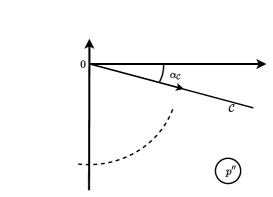
Figure 2: Contour rotation in the $p^{\prime\prime}$ complex plane. The dashed arc indicates the singularities of the partial-wave one-pion-exchange potential.

III Power counting: Leading and next-to-leading orders

In this section, we prove that the LO amplitude in all partial waves and the NLO contribution in $P$- and higher partial waves, which both do not require renormalization, satisfy the chiral power counting.

III.1 Dimensionless constants

In all our estimates, various dimensionful quantities will be expressed in terms of dimensionless constants of order one with respect to momenta and hard and soft scales. We denote them by $\mathcal{M}_{i}$, where the index $i$ indicates the origin of the constant or a quantity that it depends upon: angular momentum, order of expansion, etc. When such dimensionless constants appear in an equation, we will implicitly assume them to be of order one. In some cases, we provide explicit values or upper bounds for those constants. We do, however, not attempt to give the best estimate for such bounds because they often depend on the details of a particular scheme, whereas we want to keep the presentation general. In practice, the estimates of the relevant constants can in each particular practical case be most easily performed numerically. We further emphasize that in certain cases, additional factors of $\pi$, $4\pi$, etc., are introduced to trace back angular and momentum integrations. Finally, in some cases, we use the same names for constants in similar equations, which leads to no contradiction because one can always choose the largest constant for all considered equations.

III.2 Bounds on the potentials and the propagator

The two-nucleon propagator $G(p{;p_{\text{on}}})=m_{N}/(p_{\text{on}}^{2}-p^{2})$ is obviously bounded by

$$|G(p{;p_{\text{on}}})|\leq\mathcal{M}_{G}\frac{m_{N}}{|p^{2}|}\,,$$ (49)

with $\mathcal{M}_{G}=1/\sin(2\alpha_{\mathcal{C}})$.

Below, we list the relevant bounds on the LO and NLO potentials, which are derived in Appendix F.1 and Appendix F.2, respectively.

For the LO potentials with $l=0$ (in the case of coupled partial waves, $l$ refers to the lowest orbital angular momentum), it holds for every matrix element:

$$\left|V_{0}(p^{\prime},p)\right|<\mathcal{M}_{V_{0},0}V_{0,\text{max}}(p^{\prime},p)\,,\quad\left|V_{0}(p^{\prime},p)\right|<\mathcal{M}_{V_{0},0}V_{0,\text{max}}(p,p^{\prime})\,,$$ (50)

with

$$V_{0,\text{max}}(p^{\prime},p)=\frac{8\pi^{2}}{m_{N}\Lambda_{V}}\Big{[}F_{\tilde{\Lambda}}(|p^{\prime}|-|p|)+F_{\tilde{\Lambda}}(|p^{\prime}|)\Big{]}\,,$$ (51)

where $F_{\Lambda}(p)$ is the dipole form factor defined in Eq. (30), $\tilde{\Lambda}=\Lambda$, except for the spin-singlet partial waves without short-range leading-order interactions, for which $\tilde{\Lambda}=M_{\pi}$, and $\Lambda$ is the largest cutoff among all cutoffs used in the LO potential. Further, $\Lambda_{V}$ is the characteristic hard scale of the LO potential given by a combination of $F_{\pi}$, $m_{N}$ and the scale that governs the included contact interactions as explained in Appendix D. We explicitly keep track of $\Lambda_{V}$ and discriminate it from $\Lambda_{b}$, because the ratio $\Lambda/\Lambda_{V}$ enters most of the estimates in this work.

For the renormalizability proof in the $S$-waves carried out in the next section, we will perform subtractions of the potential. The subtraction remainders of the LO potentials with $l=0$

$$\Delta_{p}V_{0}(p^{\prime},p)\equiv V_{0}(p^{\prime},p)-V_{0}(p^{\prime},0)\,,\quad\Delta_{p^{\prime}}V_{0}(p^{\prime},p)\equiv V_{0}(p^{\prime},p)-V_{0}(0,p)\,,$$ (52)

are bounded as

$$\left|\Delta_{p}V_{0}(p^{\prime},p)\right|\leq\mathcal{M}_{V_{0},0}\left|\frac{p}{p^{\prime}}\right|^{2}V_{0,\text{max}}(p^{\prime},p)\,\,,\quad\left|\Delta_{p^{\prime}}V_{0}(p^{\prime},p)\right|\leq\mathcal{M}_{V_{0},0}\left|\frac{p^{\prime}}{p}\right|^{2}V_{0,\text{max}}(p,p^{\prime})\,\,,$$ (53)

or, alternatively, as

$$\left|\Delta_{p}V_{0}(p^{\prime},p)\right|\leq\mathcal{M}_{V_{0},0}V_{0,\text{max}}(p^{\prime},p)\,\,,\quad\left|\Delta_{p^{\prime}}V_{0}(p^{\prime},p)\right|\leq\mathcal{M}_{V_{0},0}V_{0,\text{max}}(p,p^{\prime})\,\,.$$ (54)

For $l>0$, we have the inequalities

$$\left|V_{0}(p^{\prime},p)\right|\leq\mathcal{M}_{V_{0},\tilde{l}}\left|\frac{p}{p^{\prime}}\right|^{\tilde{l}}V_{0,\text{max}}(p^{\prime},p)\,\,,\quad\left|V_{0}(p^{\prime},p)\right|\leq\mathcal{M}_{V_{0},\tilde{l}}\left|\frac{p^{\prime}}{p}\right|^{\tilde{l}}V_{0,\text{max}}(p,p^{\prime})\,\,,$$ (55)

where $\tilde{l}$ can be chosen to take any value compatible with $0\leq\tilde{l}\leq l$.

We split the NLO potential into two parts:

$$V_{2}(p^{\prime},p)=:\hat{V}_{2}(p^{\prime},p)+\tilde{V}_{2}(p^{\prime},p)\,,\quad\hat{V}_{2}(p^{\prime},p)=V_{2}(0,0)\,.$$ (56)

For the NLO potential with $l=0$, it holds:

$$\left|\hat{V}_{2}(p^{\prime},p)\right|\leq\mathcal{\hat{M}}_{V_{2},0}\frac{8\pi^{2}}{m_{N}\Lambda_{V}}\frac{M_{\pi}^{2}}{\Lambda_{b}^{2}}\,,$$ (57)

and

$$\left|\tilde{V}_{2}(p^{\prime},p)\right|{\equiv}\left|V_{2}(p^{\prime},p)-V_{2}(0,0)\right|\leq\mathcal{M}_{V_{2},0}\left(|p|^{2}+|p^{\prime}|^{2}\right)\tilde{f}_{\text{log}}(p^{\prime},p)\,,$$ (58)

with

$$\tilde{f}_{\text{log}}(p^{\prime},p) = \frac{8\pi^{2}}{m_{N}\Lambda_{V}\Lambda_{b}^{2}}f_{\text{log}}(p^{\prime},p)\,,$$

$$f_{\text{log}}(p^{\prime},p) = \theta(|p|-M_{\pi})\log\frac{|p|}{M_{\pi}}+\theta(|p^{\prime}|-M_{\pi})\log\frac{|p^{\prime}|}{M_{\pi}}+\log\frac{\tilde{\Lambda}}{M_{\pi}}+1\,.$$ (59)

For the subtraction remainders we obtain the inequalities

$$\left|\Delta_{p}\tilde{V}_{2}(p^{\prime},p)\right|\leq\mathcal{M}_{V_{2},0}|p|^{2}\tilde{f}_{\text{log}}(p^{\prime},p)\,,\quad\left|\Delta_{p^{\prime}}\tilde{V}_{2}(p^{\prime},p)\right|\leq\mathcal{M}_{V_{2},0}|p^{\prime}|^{2}\tilde{f}_{\text{log}}(p^{\prime},p)\,.$$ (60)

For $l>0$, $V_{2}(0,0)=0$ so that $\tilde{V}_{2}=V_{2}$. The employed bounds have the form

$$\left|V_{2}(p^{\prime},p)\right|\leq\mathcal{M}_{V_{2},\tilde{l}}\left|\frac{p}{p^{\prime}}\right|^{\tilde{l}}|p^{\prime}|^{2}\tilde{f}_{\text{log}}(p^{\prime},p)\,,\quad\left|V_{2}(p^{\prime},p)\right|\leq\mathcal{M}_{V_{2},\tilde{l}}\left|\frac{p^{\prime}}{p}\right|^{\tilde{l}}|p|^{2}\tilde{f}_{\text{log}}(p^{\prime},p)\,,$$ (61)

where $1\leq\tilde{l}\leq l$.

III.3 Perturbative LO amplitude

After these preparations, we are now in the position to verify the power counting for the LO partial-wave amplitude for $l>0$, which is given by the series

$$T_{0}=\sum_{n=0}^{\infty}T_{0}^{[n]}\,,\quad T_{0}^{[0]}=V_{0}\,,\quad T_{0}^{[n]}=V_{0}K^{n}\,,$$ (62)

or, more explicitly

$$\left(T_{0}^{[n]}\right)_{ji}(p^{\prime},p;p_{\text{on}})= \sum_{i_{1},\ldots,i_{n}=1}^{n_{\text{PW}}}\int\prod_{k=1}^{n}\frac{p_{k}^{2}dp_{k}}{(2\pi)^{3}}\left(V_{0}\right)_{ji_{1}}(p^{\prime},p_{1})K_{i_{1},i_{2}}(p_{1},p_{2};p_{\text{on}})\dots K_{i_{n}i}(p_{n},p;p_{\text{on}})\,,$$ (63)

where the subscripts of $T_{0}$, $V_{0}$ and $K$ denote the partial wave index and $n_{\text{PW}}=1,2$ is the number of channels. We are now going to show by induction that

$$\left|T_{0}^{[n]}(p^{\prime},p;p_{\text{on}})\right|\leq\mathcal{M}_{n}\frac{8\pi^{2}}{m_{N}\Lambda_{V}}\,.$$ (64)

From Eq. (55) with $\tilde{l}=0$, it follows that

$$\mathcal{M}_{0}=2\mathcal{M}_{V_{0},0}\,.$$ (65)

Assuming that Eq. (64) holds and applying the bound (55) with $\tilde{l}=0$, we get for $T_{0}^{[n+1]}$ (here, we suppress the channel indices):

$$\left|T_{0}^{[n+1]}(p^{\prime},p;p_{\text{on}})\right| = \left|\int\frac{p^{\prime\prime 2}dp^{\prime\prime}}{(2\pi)^{3}}T_{0}^{[n]}(p^{\prime},p^{\prime\prime};p_{\text{on}})G(p^{\prime\prime};p_{\text{on}})V_{0}(p^{\prime\prime},p)\right|$$ (66)

$$\leq \frac{8\pi^{2}\mathcal{M}_{n}}{m_{N}\Lambda_{V}}n_{\text{PW}}\mathcal{M}_{V_{0},0}\int\frac{|p^{\prime\prime}|^{2}d|p^{\prime\prime}|}{(2\pi)^{3}}\left|G(p^{\prime\prime};p_{\text{on}})\right|V_{0,\text{max}}(p^{\prime\prime},p)$$

$${\equiv} \frac{8\pi^{2}\mathcal{M}_{n}}{m_{N}\Lambda_{V}}n_{\text{PW}}\mathcal{M}_{V_{0},0}I_{V_{0}}(p^{\prime},p;p_{\text{on}})$$

$$\leq \frac{8\pi^{2}\mathcal{M}_{n}}{m_{N}\Lambda_{V}}n_{\text{PW}}\mathcal{M}_{V_{0},0}\mathcal{M}_{I_{V_{0}}}\frac{\tilde{\Lambda}}{\Lambda_{V}}\,.$$

The integral $I_{V_{0}}(p^{\prime},p;p_{\text{on}})$ is estimated in Appendix G. Introducing the quantity

$$\Sigma=n_{\text{PW}}\mathcal{M}_{V_{0},0}\mathcal{M}_{I_{V_{0}}}\frac{\tilde{\Lambda}}{\Lambda_{V}}\,,$$ (67)

we finally arrive at the following bound

$$\left|T_{0}^{[n]}(p_{\text{on}})\right|\leq\frac{8\pi^{2}}{m_{N}\Lambda_{V}}\mathcal{M}_{0}\,\Sigma^{n}\,.$$ (68)

For spin-triplet partial waves and for spin-singlet partial waves featuring a short-range LO interaction, all terms $T_{0}^{[n]}$ are, as expected, of order $\mathcal{O}(Q^{0})$ as long as the cutoff is of the order of the hard scale, $\Lambda\sim\Lambda_{V}$. If $\Sigma<1$, the series for $T_{0}$ is perturbative, although for $\Sigma$ close to $1$, the convergence of this series might be very slow. Obviously, the convergence gets better for smaller values of $\Lambda$ until the cutoff artifacts become relevant. For spin-singlet partial waves without short-range LO interactions, we have a better convergence, $T_{0}^{[n]}\sim\left(M_{\pi}/\Lambda\right)^{n}$, because the integrals converge at momenta $p\sim M_{\pi}$.

We do not provide here the estimates for $\Sigma$ for individual partial waves although it is obvious that $\Sigma$ will get smaller for larger values of $l$. It is also straightforward to obtain a better bound for $T_{0}^{[n]}$ for spin-triplet channels and spin-singlet channels with short-range interactions when $n<2l$, so that the unregularized loop integrals are ultraviolet convergent, by applying Eq. (55) with $\tilde{l}=l$ for the integration regions $|p^{\prime\prime}|\geq p_{\text{on}}$:

$$\left|T_{0}^{[n]}(p_{\text{on}})\right|\leq\frac{8\pi^{2}}{m_{N}\Lambda_{V}}\mathcal{\tilde{M}}_{n,l}\left(\frac{p_{\text{on}}}{\Lambda_{V}}\right)^{n}\,.$$ (69)

However, this does not affect our general conclusions about the validity of the power counting.

III.4 Perturbative amplitude at NLO: Higher partial waves

In a complete analogy with the previous section, we can analyze the NLO amplitude of order $m+n$ in $V_{0}$:

$$T_{2}^{[m,n]}=\bar{K}^{m}V_{2}K^{n}\,,$$ (70)

for partial waves with $l\geq 1$. In the following, we will show by induction that

$$\left|T_{2}^{[m,n]}(p^{\prime},p;p_{\text{on}})\right|\leq\mathcal{M}_{T_{2}}^{m,n}|p^{\prime}||p|\tilde{f}_{\text{log}}(p^{\prime},p)\,.$$ (71)

From Eq. (61) with $\tilde{l}=1$, it follows

$$\mathcal{M}_{T_{2}}^{0,0}=\mathcal{M}_{V_{2},1}\,.$$ (72)

Assuming that Eq. (71) holds and applying the bound (55) with $\tilde{l}=1$, we obtain for $T_{2}^{[m,n+1]}$:

$$\left|T_{2}^{[m,n+1]}(p^{\prime},p{;p_{\text{on}}})\right| = \left|\int\frac{p^{\prime\prime 2}dp^{\prime\prime}}{(2\pi)^{3}}T_{2}^{[m,n]}(p^{\prime},p^{\prime\prime}{;p_{\text{on}}})G(p^{\prime\prime}{;p_{\text{on}}})V_{0}(p^{\prime\prime},p)\right|$$ (73)

$$\leq n_{\text{PW}}\mathcal{M}_{T_{2}}^{m,n}\mathcal{M}_{V_{0},1}\int\frac{|p^{\prime\prime}|^{2}dp^{\prime\prime}}{(2\pi)^{3}}|p^{\prime}||p^{\prime\prime}|\tilde{f}_{\text{log}}(p^{\prime},p^{\prime\prime})\left|G(p^{\prime\prime}{;p_{\text{on}}})\right|\left|\frac{p}{p^{\prime\prime}}\right|V_{0,\text{max}}(p^{\prime},p)$$

$$\leq n_{\text{PW}}\mathcal{M}_{T_{2}}^{m,n}\mathcal{M}_{V_{0},1}|p^{\prime}||p|\int\frac{|p^{\prime\prime}|^{2}dp^{\prime\prime}}{(2\pi)^{3}}\tilde{f}_{\text{log}}(p^{\prime},p^{\prime\prime})\left|G(p^{\prime\prime}{;p_{\text{on}}})\right|V_{0,\text{max}}(p^{\prime},p)$$

$${\equiv} n_{\text{PW}}\mathcal{M}_{T_{2}}^{m,n}\mathcal{M}_{V_{0},1}|p^{\prime}||p|I_{f_{\text{log}}}(p^{\prime},p{;p_{\text{on}}})$$

$$\leq n_{\text{PW}}\mathcal{M}_{T_{2}}^{m,n}\mathcal{M}_{V_{0},1}\mathcal{M}_{f_{\text{log}}}\frac{\tilde{\Lambda}}{\Lambda_{V}}|p^{\prime}||p|\tilde{f}_{\text{log}}(p^{\prime},p)\,,$$

and, analogously, for $T_{2}^{[m+1,n]}$. The integral $I_{f_{\text{log}}}(p^{\prime},p{;p_{\text{on}}})$ is estimated in Appendix G. Introducing

$$\Sigma_{1}=n_{\text{PW}}\mathcal{M}_{V_{0},1}\mathcal{M}_{f_{\text{log}}}\frac{\tilde{\Lambda}}{\Lambda_{V}}\,,$$ (74)

we obtain

$$\mathcal{M}_{T_{2}}^{m,n}=\mathcal{M}_{V_{2},1}\Sigma_{1}^{m+n}\,.$$ (75)

Therefore, for the on-shell kinematics with $p=p^{\prime}=p_{\text{on}}$, the amplitude $T_{2}^{[m,n]}(p_{\text{on}})$ is bounded by

$$\left|T_{2}^{[m,n]}(p_{\text{on}})\right|\leq\frac{8\pi^{2}\mathcal{M}_{V_{2},1}}{m_{N}\Lambda_{V}}\Sigma_{1}^{m+n}\frac{p_{\text{on}}^{2}}{\Lambda_{b}^{2}}f_{\text{log}}(p_{\text{on}},p_{\text{on}})\,,$$ (76)

where we have used Eq. (59). For the spin-triplet partial waves and for the spin-singlet partial waves with a short-range LO interaction, we get

$$\left|T_{2}^{[m,n]}(p_{\text{on}})\right|\leq\frac{8\pi^{2}\mathcal{M}_{V_{2},1}}{m_{N}\Lambda_{V}}\Sigma_{1}^{m+n}\frac{p_{\text{on}}^{2}}{\Lambda_{b}^{2}}\,\log{\frac{\Lambda}{M_{\pi}}}\,,$$ (77)

where we have used $p_{\text{on}}\leq\mathcal{M}_{p_{\text{on}}}M_{\pi}$ and absorbed terms of order $1$ into the $\log\Lambda/M_{\pi}$-term in $f_{\text{log}}(p_{\text{on}},p_{\text{on}})$, thereby redefining $\mathcal{M}_{V_{2},1}$. If we choose the cutoff to be of the order of the hard scale $\Lambda\sim\Lambda_{V}$, all terms $T_{2}^{[m,n]}$ are of order $\mathcal{O}(Q^{2}\log Q)$ and do not violate power counting. The appearance of the $\log\Lambda/M_{\pi}$-factor in Eq. (77) as compared to the bare potential $V_{2}$ can be traced back to the $\log p/M_{\pi}$ terms in $V_{2}$ and the fact that the integrals converge at momenta $p\sim\Lambda$. As in the case of the leading order amplitude, one can improve the bounds on $T_{2}^{[m,n]}$ for $n+m<2l$ using Eqs.(61), (55) for the integration momenta $|p^{\prime\prime}|\geq p_{\text{on}}$. This does not modify our findings about the power counting for the NLO amplitude either.

For spin-singlet partial waves without short-range LO interactions, where the integrals converge at $|p^{\prime\prime}|\sim M_{\pi}$, we have

$$\left|T_{2}^{[m,n]}(p_{\text{on}})\right|\leq\frac{8\pi^{2}\mathcal{M}_{V_{2},1}}{m_{N}\Lambda_{V}}\Sigma_{1}^{m+n}\frac{p_{\text{on}}^{2}}{\Lambda_{b}^{2}}\,,$$ (78)

which gives

$$T_{2}^{[m,n]}\sim\frac{p_{\text{on}}^{2}}{\Lambda_{b}^{2}}\left(\frac{M_{\pi}}{\Lambda_{V}}\right)^{m+n}\,.$$

To summarize, we have shown in this section that (i) the LO scattering amplitude scales according to the power counting and (ii) the NLO contribution to the amplitude in $P$- and higher partial waves does not contain power-counting breaking terms, i.e. it is also compatible with the power counting.

IV Perturbative renormalization of the amplitude at NLO: $S$-waves

In this section, we consider the renormalization of the next-to-leading-order amplitude in the $S$-waves, i.e. in the partial waves where the power-counting breaking terms have to be absorbed by the counter terms.

As specified in Eq. (56), the next-to-leading order $S$-wave partial wave potential is split into two parts $V_{2}(p^{\prime},p)=\hat{V}_{2}(p^{\prime},p)+\tilde{V}_{2}(p^{\prime},p)$ ($V_{2}$ is a matrix of dimension $n_{\text{PW}}\times n_{\text{PW}}$ with $n_{\text{PW}}=1$ for ${}^{1}S_{0}$ and $n_{\text{PW}}=2$ for ${}^{3}S_{1}-{{}^{3}D}_{1}$ system). Analogously, for the $T$-matrix, we define:

$$\hat{T}_{2}^{[m,n]}=\bar{K}^{m}\hat{V}_{2}K^{n}\,,\quad\tilde{T}_{2}^{[m,n]}=\bar{K}^{m}\tilde{V}_{2}K^{n}\,.$$ (79)

The amplitude $\hat{T}_{2}^{[m,n]}$ can be estimated in the same way as $T_{0}$ using Eq. (57), first obtaining the bounds for $\hat{T}_{2}^{[0,n]}$:

$$\left|\hat{T}_{2}^{[0,n]}(p_{\text{on}})\right|\leq\mathcal{\hat{M}}_{V_{2},0}\frac{8\pi^{2}}{m_{N}\Lambda_{V}}\frac{M_{\pi}^{2}}{\Lambda_{b}^{2}}\,\Sigma^{n}\,,$$ (80)

and then symmetrically for $\hat{T}_{2}^{[m,n]}$:

$$\left|\hat{T}_{2}^{[m,n]}(p_{\text{on}})\right|\leq\mathcal{\hat{M}}_{V_{2},0}\frac{8\pi^{2}}{m_{N}\Lambda_{V}}\frac{M_{\pi}^{2}}{\Lambda_{b}^{2}}\Sigma^{m+n}\,.$$ (81)

IV.1 Subtractions in the BPHZ scheme

The amplitude $\tilde{T}_{2}^{[m,n]}$ contains power-counting breaking contributions from the integration regions where all or some of the loop momenta are $p\sim\Lambda$. It is natural to expect that such contributions can be removed by performing subtractions in all possible subdiagrams in the spirit of the Bogoliubov-Parasiuk-Hepp-Zimmermann (BPHZ) renormalization procedure Bogoliubov and Parasiuk (1957); Hepp (1966); Zimmermann (1969) (for a detailed discussion of the BPHZ scheme see Refs. Collins (1986); Zavialov (1990); Smirnov (1991)). In the following, we will show that removing all power-counting breaking terms in $\tilde{T}_{2}^{[m,n]}$ can be achieved by introducing the appropriate momentum independent counter terms $\delta V^{(2)}_{C_{S}}$ and $\delta V^{(2)}_{C_{T}}$, or, equivalently, $\delta V^{(2)}_{{}^{1}S_{0}}$ and $\delta V^{(2)}_{{}^{3}S_{1}}$.

In the present work, we consider for simplicity subtractions at zero momenta and introduce the linear operation for the overall subtraction $\mathds{T}$ that replaces an operator $X$ with matrix elements $X_{ji}(p^{\prime},p{;p_{\text{on}}})$ with its value at $p=p^{\prime}=p_{\text{on}}=0$:

$$\mathds{T}(X)=X_{11}(0,0,0)V_{\text{ct}}\,,$$ (82)

where $V_{\text{ct}}$ is the contact operator $\left(V_{\text{ct}}\right)_{ji}(p^{\prime},p)=\delta_{1,i}\delta_{1,j}$. For convenience, we also introduce the operation $\mathds{\bar{T}}=\mathds{1-T}$:

$$\mathds{\bar{T}}(X)=X-\mathds{T}(X).$$ (83)

Since the leading order amplitude does not violate power counting (see Sec. III.3), the subgraphs leading to power-counting violating terms must necessarily include the vertex $\tilde{V}_{2}$ and have the form $\bar{K}^{m_{1}}\tilde{V}_{2}K^{n_{1}}=\tilde{T}_{2}^{[m_{1},n_{1}]}$ for some $m_{1}$, $n_{1}$. We denote the diagram corresponding to the amplitude $\tilde{T}_{2}^{[m,n]}$ as $(m,n)$ and define the subtraction operation $\mathds{T}^{m_{1},n_{1}}$ for a subgraph $(m_{1},n_{1})$, $m_{1}\leq m$, $n_{1}\leq n$:

$$\mathds{T}^{m_{1},n_{1}}(\tilde{T}_{2}^{[m,n]})=\bar{K}^{m-m_{1}}\mathds{T}(\tilde{T}_{2}^{[m_{1},n_{1}]})K^{n-n_{1}}\,.$$ (84)

A composition of two subtractions is defined analogously:

$$\mathds{T}^{m_{2},n_{2}}\big{(}\mathds{T}^{m_{1},n_{1}}(\tilde{T}_{2}^{[m,n]})\big{)}=\bar{K}^{m-m_{2}}\mathds{T}\big{(}\bar{K}^{m_{2}-m_{1}}\mathds{T}(\tilde{T}_{2}^{[m_{1},n_{1}]})K^{n_{2}-n_{1}}\big{)}K^{n-n_{2}}\,,$$ (85)

where $m_{1}\leq m_{2}\leq m$, $n_{1}\leq n_{2}\leq n$ and either $m_{1}<m_{2}$ or $n_{1}<n_{2}$.

The BPHZ $\mathds{R}$-operation that leads to a renormalized expression for $\tilde{T}_{2}^{[m,n]}$ is given by

$$\mathds{R}(\tilde{T}_{2}^{[m,n]})=\tilde{T}_{2}^{[m,n]}+\sum_{U_{k}\in\mathcal{F}^{m,n}}\bigg{(}\prod_{(m_{i},n_{i})\in U_{k}}-\mathds{T}^{m_{i},n_{i}}\bigg{)}\tilde{T}_{2}^{[m,n]}\,,$$ (86)

where $\mathcal{F}^{m,n}$ represents the set of all forests, i.e, the set of all possible distinct sequences of nested subdiagrams $(m_{i},n_{i})$:

$$U_{k}=((m_{k;1},n_{k;1}),(m_{k;2},n_{k;2}),\dots)\,,$$

$$m\geq m_{k;i+1}\geq m_{k;i}\geq 0\,,\quad n\geq n_{k;i+1}\geq n_{k;i}\geq 0\,,\quad n+m>0\,,$$ (87)

where the last inequality can be omitted because $\tilde{T}_{2}^{[0,0]}(0,0,0)=\tilde{V}_{2}(0,0)=0$ and, therefore, $\mathds{T}^{0,0}(\tilde{T}_{2}^{[m,n]})=0$. For instance, the set $\mathcal{F}^{1,1}$ contains the following forests:

$$U_{1}=((0,1))\,,\quad U_{2}=((0,1),(1,1))\,,\quad U_{3}=((1,0))\,,\quad U_{4}=((1,0),(1,1))\,,\quad U_{5}=((1,1))\,.$$ (88)

When proving the power counting for $\mathds{R}(\tilde{T}_{2}^{[m,n]})$, we will also use an equivalent representation of the $\mathds{R}$-operation Anikin et al. (1973); Smirnov (1991); Zavialov (1990); Bogolyubov and Shirkov (1959):

$$\mathds{R}\left(\tilde{T}_{2}^{[m,n]}\right)=\vdots\bigg{(}\prod_{m_{i}=0}^{m}\prod_{n_{j}=0}^{n}\mathds{\bar{T}}^{m_{i},n_{j}}\bigg{)}\tilde{T}_{2}^{[m,n]}\,\vdots=\vdots\bigg{[}\prod_{m_{i}=0}^{m}\prod_{n_{j}=0}^{n}\left(\mathds{1}-\mathds{T}^{m_{i},n_{j}}\right)\bigg{]}\tilde{T}_{2}^{[m,n]}\,\vdots\,,$$ (89)

where the three-dot-product means that overlapping subdiagrams (i.e. $(m_{1},n_{1})$ and $(m_{2},n_{2})$ such that $m_{2}>m_{1}$ and $n_{2}<n_{1}$ or $n_{2}>n_{1}$ and $m_{2}<n_{1}$) should be dropped from the product after expanding the brackets. The ordering of $\mathds{T}^{m_{i},n_{j}}$ in any product is such that $\mathds{T}$ corresponding to smaller subdiagrams (with smaller $m_{i}$ or $n_{j}$) are applied first, e.g. $\mathds{T}^{4,5}\mathds{T}^{3,2}\mathds{T}^{1,2}$.

The presence of the overlapping diagrams prevents one from directly applying the recurrent procedure we used in the case of higher partial waves except for the cases of $\tilde{T}_{2}^{[m,0]}$ and $\tilde{T}_{2}^{[0,n]}$. In particular, the residues $\Delta_{p}\mathds{R}(\tilde{T}_{2}^{[m,n]})$ and $\Delta_{p^{\prime}}\mathds{R}(\tilde{T}_{2}^{[m,n]})$ do not satisfy the same inequalities as $\tilde{V}_{2}$, only some parts of them do. As we will see later in this section, the correct way to estimate $\mathds{R}(\tilde{T}_{2}^{[m,n]})$ is not the induction from $\mathds{R}(\tilde{T}_{2}^{[m,n-1]})$ or from $\mathds{R}(\tilde{T}_{2}^{[m-1,n]})$, but rather from some combination of the two.

In an analysis of the renormalized amplitude in the BPHZ scheme, one typically performs a decomposition of the integration region into sectors, usually, in the parametric representation Hepp (1966); Speer (1975) (see also Refs. Heinrich (2008); Smirnov and Smirnov (2009) for more recent applications). In our case, we would like to keep a rather general form of the interaction and the regulator, and it appears convenient to decompose the whole integration region into sectors in momentum space as described in the next subsection. For the examples of splitting the integration in momentum space into subregions in the analysis of Feynman integrals we refer the reader to Refs. Weinberg (1960); Hahn and Zimmermann (1968); Caswell and Kennedy (1983).

IV.2 Sector decomposition

In this subsection, we describe the sector decomposition of the whole $(m+n)$-dimensional integration region that allows one to prove that the BPHZ procedure indeed leads to the renormalized amplitude satisfying the power counting.

We denote the momenta of $\bar{K}^{m}\tilde{V}_{2}K^{n}$ corresponding to the loops involving $K$ as $p_{1}$, $p_{2},\,\dots,\,p_{n}$ ($p_{n+1}\equiv p$) starting with the loop closest to $V_{2}$. Analogously, we denote the momenta corresponding to the loops with $\bar{K}$ as $p^{\prime}_{1}$, $p^{\prime}_{2},\,\dots,\,p^{\prime}_{m}$ ($p^{\prime}_{m+1}\equiv p^{\prime}$). This means:

$$\tilde{T}_{2}^{[m,n]}(p^{\prime},p{;p_{\text{on}}})=\int\prod_{i=1}^{n}\prod_{j=1}^{m}\frac{p_{i}^{2}dp_{i}}{(2\pi)^{3}}\frac{p^{\prime 2}_{j}dp^{\prime}_{j}}{(2\pi)^{3}}\bar{K}(p^{\prime},p^{\prime}_{m})\dots\bar{K}(p^{\prime}_{2},p^{\prime}_{1})\tilde{V}_{2}(p^{\prime}_{1},p_{1})K(p_{1},p_{2})\dots K(p_{n},p)\,.$$ (90)

We represent $\tilde{T}_{2}^{[m,n]}$ as a sum

$$\tilde{T}_{2}^{[m,n]}=\sum_{i}\tilde{T}_{2}^{\mathcal{P}_{i}^{m,n}}\,,$$ (91)

where the sum runs over all paths $\mathcal{P}_{i}^{m,n}$ that have the form of sequences of momenta

$$\mathcal{P}_{1}^{m,n}=(p_{1},\dots,p_{n},p^{\prime}_{1},\dots p^{\prime}_{m})\,,\quad\mathcal{P}_{2}^{m,n}=(p_{1},\dots,p_{n-1},p^{\prime}_{1},p_{n},p_{2}^{\prime},\dots p^{\prime}_{m})\,,\quad\ldots\,,$$ (92)

with all ${n+m\choose n}$ possible permutations of $p_{i}$ and $p^{\prime}_{j}$ in Eq. (92) that do not change the order within $p_{i}$ and $p^{\prime}_{j}$. I.e., for $j_{1}>j_{2}$, $p_{j_{1}}$ appears to the right of $p_{j_{2}}$, and analogously for $p^{\prime}$, e.g. $(p_{1},p_{2},p^{\prime}_{1},p_{3},p_{4},p^{\prime}_{2},p^{\prime}_{3},p^{\prime}_{4},p^{\prime}_{5})$. To each path $\mathcal{P}_{i}$, we assign different $(n+m)$-dimensional integration sectors $\mathcal{D}_{i}^{m,n}=\mathcal{D}(\mathcal{P}_{i}^{m,n})$. The choice of the integration sectors for a path $\mathcal{P}_{i}$ is as follows: if $p_{k}^{\prime}$ in $\mathcal{P}_{i}$ is immediately preceded by $r$ variables $p_{j},\dots,p_{j+r-1}$, then the following $r$ inequalities must hold:

$$|p_{k}^{\prime}|\leq|p_{j}|\,,\;\dots\,,\;|p_{k}^{\prime}|\leq|p_{j+r-1}|\,,$$ (93)

and, conversely, if $p_{k}$ is immediately preceded by $r$ variables $p^{\prime}_{j},\dots,p^{\prime}_{j+r-1}$, then

$$|p_{k}|\leq|p^{\prime}_{j}|\,,\;\dots\,,\;|p_{k}|\leq|p^{\prime}_{j+r-1}|\,.$$ (94)

If $p_{k}$ ($p^{\prime}_{k}$) is preceded by $p_{k-1}$ ($p^{\prime}_{k-1}$) or is the first momentum in the path, then there are no constraints imposed on such a momentum. The motivation for this choice of sectors will become clear during the proof of the renormalizability of $\tilde{T}_{2}^{[m,n]}$ and the analysis of the overlapping diagrams.

We denote the set of all $\mathcal{P}_{i}^{m,n}$ as $\mathcal{S}^{m,n}\equiv\{\mathcal{P}_{i}^{m,n}\}$. The corresponding sectors $\{\mathcal{D}_{i}^{m,n}\}$ do not overlap (except along the boundaries), and their union covers the whole integration region. We will show this below by induction.

The case of $\mathcal{S}^{0,n}$ is trivial. Assume that the statement holds for $\mathcal{S}^{m,n}$. The set $\mathcal{S}^{m,n}$ can be split into the following subsets:

$$\mathcal{S}^{m,n}=\bigcup_{k=0,n}\mathcal{S}^{m,n}_{k}\,,\quad\mathcal{S}^{m,n}_{k}=\{\mathcal{P}^{m,n}_{i_{k}}\}\,,$$ (95)

where $i_{k}$ runs over the sequences that end with exactly $k$ momenta $p_{j}$: $p_{n-k+1},\dots,p_{n}$. Then, the set $\mathcal{S}^{m+1,n}$ is given by

$$\mathcal{S}^{m+1,n}=\{\mathcal{P}^{m+1,n}_{i}\}=\bigcup_{k=0}^{n}\mathcal{\tilde{S}}^{m+1,n}_{k}\,,\quad\text{where}\;\;\;\mathcal{\tilde{S}}^{m+1,n}_{k}=\bigcup_{j=0}^{k}\{\mathcal{P}^{m+1,n}_{i_{k},\,j}\}\,,$$ (96)

where the sequence $\mathcal{P}^{m+1,n}_{i_{k},\,j}$ is obtained from $\mathcal{P}^{m,n}_{i_{k}}$ by inserting the momentum $p^{\prime}_{m+1}$ into the $(k-j+1)$-th position from the right, i.e. into the $(n+m+1-k+j)$-th position. The union over $j$ of the sectors corresponding to $\mathcal{P}^{m+1,n}_{i_{k},\,j}$ is determined by the sector $\mathcal{D}\left(\mathcal{P}^{m+1,n}_{i_{k}}\right)$ and arbitrary $p^{\prime}_{m+1}$:

$$\bigcup_{j=0}^{k}\mathcal{D}\left(\mathcal{P}^{m+1,n}_{i_{k},\,j}\right)=\mathcal{D}\left(\mathcal{P}^{m,n}_{i_{k}}\right)\times\left\{p^{\prime}_{m+1}\in\mathcal{C}\right\}\,,$$ (97)

which can be shown as follows.

The sector $\mathcal{D}\left(\mathcal{P}^{m+1,n}_{i_{k},\,0}\right)$ is determined by (here $k>0$, the case $k=0$ is trivial)

$$\mathcal{D}\left(\mathcal{P}^{m+1,n}_{i_{k},\,0}\right)=\mathcal{D}\left(\mathcal{P}^{m,n}_{i_{k}}\right)\times\left\{p^{\prime}_{m+1}\Big{|}|p^{\prime}_{m+1}|\leq|p_{n}|,\;\dots\,,\;|p^{\prime}_{m+1}|\leq|p_{n-k+1}|\right\}\,.$$ (98)

It is easy to prove by induction that for $0\leq l<k$,

$$\bigcup_{j=0}^{l}\mathcal{D}\left(\mathcal{P}^{m+1,n}_{i_{k},\,j}\right)=\mathcal{D}\left(\mathcal{P}^{m,n}_{i_{k}}\right)\times\left\{p^{\prime}_{m+1}\Big{|}|p^{\prime}_{m+1}|\leq|p_{n-l}|,\;\dots\,,\;|p^{\prime}_{m+1}|\leq|p_{n-k+1}|\right\}\,.$$ (99)

Indeed, assuming Eq. (99) is fulfilled, we obtain

$$\bigcup_{j=0}^{l+1}\mathcal{D}\left(\mathcal{P}^{m+1,n}_{i_{k},\,j}\right) = \bigcup_{j=0}^{l}\mathcal{D}\left(\mathcal{P}^{m+1,n}_{i_{k},\,j}\right)\cup\mathcal{D}\left(\mathcal{P}^{m+1,n}_{i_{k},\,l+1}\right)$$ (100)

$$= \mathcal{D}\left(\mathcal{P}^{m,n}_{i_{k}}\right)\times\left\{p^{\prime}_{m+1}\Big{|}|p^{\prime}_{m+1}|\leq|p_{n-l}|,\;\dots\,,\;|p^{\prime}_{m+1}|\leq|p_{n-k+1}|\right\}$$

$${}\cup\mathcal{D}\left(\mathcal{P}^{m,n}_{i_{k}}\right)\times\left\{p^{\prime}_{m+1}\Big{|}|p^{\prime}_{m+1}|\leq|p_{n-l-1}|,\;\dots\,,\;|p^{\prime}_{m+1}|\leq|p_{n-k+1}|,|p^{\prime}_{m+1}|\geq|p_{n-l}|\right\}$$

$$= \mathcal{D}\left(\mathcal{P}^{m,n}_{i_{k}}\right)\times\left\{p^{\prime}_{m+1}\Big{|}|p^{\prime}_{m+1}|\leq|p_{n-l-1}|,\dots\,,|p^{\prime}_{m+1}|\leq|p_{n-k+1}|\right\}\,.$$

Therefore,

$$\bigcup_{j=0}^{k-1}\mathcal{D}\left(\mathcal{P}^{m+1,n}_{i_{k},\,j}\right)=\mathcal{D}\left(\mathcal{P}^{m,n}_{i_{k}}\right)\times\left\{p^{\prime}_{m+1}\Big{|}|p^{\prime}_{m+1}|\leq|p_{n-k+1}|\right\}\,.$$ (101)

On the other hand,

$$\mathcal{D}\left(\mathcal{P}^{m+1,n}_{i_{k},\,k}\right)=\mathcal{D}\left(\mathcal{P}^{m,n}_{i_{k}}\right)\times\left\{p^{\prime}_{m+1}\Big{|}|p^{\prime}_{m+1}|\geq|p_{n-k+1}|\right\}\,,$$ (102)

since in $\mathcal{P}^{m+1,n}_{i_{k},\,k}$, the momentum $p_{n-k+1}$ is preceded by $p^{\prime}_{m+1}$, $p^{\prime}_{m}$ and other $p^{\prime}_{r}$ that stay in $\mathcal{P}^{m,n}_{i_{k}}$ in front of $p^{\prime}_{m}$. Equations (101), (102) yield Eq. (97), which together with Eq. (96) proves the completeness of the partitions $\mathcal{S}^{m+1,n}$ and completes the induction.

The subtraction operation $\mathds{T}^{m_{1},n_{1}}$ for $\tilde{T}_{2}^{\mathcal{P}_{i}^{m,n}}$ is defined as in Eq. (84), where the integration region in

$$\bar{K}^{m-m_{1}}V_{\text{ct}}K^{n-n_{1}}$$ (103)

is constrained by those inequalities from Eqs. (93), (94) that relate the momenta $\{p^{\prime}_{m_{1}+1},\dots,p^{\prime}_{m},p_{n_{1}+1},\dots,p_{n}\}$ among each other, whereas the integration region in

$$\tilde{T}_{2}^{[m_{1},n_{1}]}(p^{\prime}_{m_{1}+1}=0,p_{n_{1}+1}=0,p_{\text{on}}=0)$$ (104)

is constrained by the inequalities from Eqs. (93), (94) that relate the momenta $\{p^{\prime}_{1},\dots,p^{\prime}_{m_{1}+1},p_{1},\dots,p_{n_{1}+1}\}$ among each other. Since in Eq. (104), $p^{\prime}_{m_{1}+1}=0$ and $p_{n_{1}+1}=0$, any inequality involving $p^{\prime}_{m_{1}+1}$ or $p_{n_{1}+1}$ is either satisfied automatically (if $|p_{i}|\geq|p^{\prime}_{m_{1}+1}|$ or $|p^{\prime}_{j}|\geq|p_{n_{1}+1}|$) or makes the whole integral vanish (if $|p_{i}|\leq|p^{\prime}_{m_{1}+1}|$ or $|p^{\prime}_{j}|\leq|p_{n_{1}+1}|$). Analogously, for the subsequent subtractions (see Eq. (85)), only the momenta entering into the remaining integration in

$$\bar{K}^{m-m_{2}}V_{\text{ct}}K^{n-n_{2}}$$ (105)

are constrained. That such partitions of the integration regions in the subtracted amplitudes cover the whole space and do not overlap will be seen in the next subsection.

IV.3 Overlapping diagrams

Now, we will show how the paths $\mathcal{P}_{i}^{m,n}$ and the corresponding sectors $\mathcal{D}\left(\mathcal{P}_{i}^{m,n}\right)$ help disentangling overlapping diagrams.

First, we associate with the sequence $\mathcal{P}_{i}^{m,n}$ the maximal forest $U_{\text{max}}(\mathcal{P}^{m,n}_{i})$ (a maximal forest is a forest that is not contained in any other forest) as follows:

$$U_{\text{max}}(\mathcal{P}^{m,n}_{i})=((m_{i;1},n_{i;1}),\,(m_{i;2},n_{i;2}),\,\dots,\,(m_{i;m+n},n_{i;m+n}))\,,\quad\text{with}\;\;\quad m_{i;m+n}=m\,,\quad n_{i;m+n}=n\,,$$ (106)

where $m_{i;k}=m_{i;k-1}+1$, $n_{i;k}=n_{i;k-1}$ if the $k$-th element of $\mathcal{P}^{m,n}_{i}$ is $p_{r}^{\prime}$, $(\mathcal{P}^{m,n}_{i})_{k}=p_{r}^{\prime}$ (for some $r$), and $m_{i;k}=m_{i;k-1}$, $n_{i;k}=n_{i;k-1}+1$ if $(\mathcal{P}^{m,n}_{i})_{k}=p_{s}$ (for some $s$). By definition, $m_{i;0}=n_{i;0}=0$. We denote by $\mathcal{F}^{m,n}_{i}$ the set of forests that consists of all subsequences of $U_{\text{max}}(\mathcal{P}^{m,n}_{i})$. All subdiagrams of the diagram $(m,n)$ that belong to $U_{\text{max}}(\mathcal{P}^{m,n}_{i})$ are non-overlapping.

Assume that a subdiagram $(p,q)$ of the diagram $(m,n)$ does not belong to any forest in $\mathcal{F}(\mathcal{P}^{n,m}_{i})$, i.e. it does not belong to the maximal forest $U_{\text{max}}(\mathcal{P}^{m,n}_{i})=((m_{i;1},n_{i;1}),\,\ldots,\,(m_{i;k},n_{i;k}),\,\ldots,\,(m_{i;m+n},n_{i;m+n}))$. Therefore,

$$\nexists k:\quad m_{i;k}=p\text{ and }n_{i;k}=q\,.$$ (107)

For some $k=k_{0}$, the subdiagram $(m_{i;k_{0}},n_{i;k_{0}})$ starts to overlap with the subdiagram $(p,q)$. Two symmetric cases are possible:

$$p<m\,,\quad q\leq n\,,\quad m_{i;k_{0}-1}=p\,,\ m_{i;k_{0}}=p+1\,,\quad n_{i;k_{0}}<q\,,$$ (108)

or

$$p\leq m\,,\quad q<n\,,\quad n_{i;k_{0}-1}=q\,,\ n_{i;k_{0}}=q+1\,,\quad m_{i;k_{0}}<p\,.$$ (109)

Consider, for definiteness, the former case (the latter case can be treated analogously). Since $n_{i;k_{0}}<q\leq n$, there exists $k_{1}>k_{0}$ such that

$$\text{for }k_{0}\leq k<k_{1}:\quad n_{i;k}=n_{i;k_{0}}\,\text{ and }n_{i;k_{1}}=n_{i;k_{0}}+1\,.$$ (110)

From the definitions of the sectors given in the previous subsection, it follows that in $\mathcal{D}\left(\mathcal{P}_{i}^{m,n}\right)$, $|p_{n_{i;k_{1}}}|\leq|p^{\prime}_{m_{i;k_{0}}}|=|p^{\prime}_{p+1}|$.

The subtraction operation $\mathds{T}^{(p,q)}$ for $\tilde{T}_{2}^{\mathcal{P}_{i}^{m,n}}$ gives

$$\mathds{T}^{p,q}\left(\tilde{T}_{2}^{\mathcal{P}_{i}^{m,n}}\right)=(\bar{K})^{m-p}\tilde{T}_{2}^{[p,q]}(p^{\prime}_{p+1}=0,p_{q+1}=0,p_{\text{on}}=0)V_{\text{ct}}K^{n-q}\,,$$ (111)

where the integration region is constrained, in particular, by $|p_{n_{i,k_{1}}}|\leq|p^{\prime}_{p+1}|=0$, which makes the whole integral vanish:

$$\mathds{T}^{p,q}\left(\tilde{T}_{2}^{\mathcal{P}_{i}^{m,n}}\right)=0\,.$$ (112)

The same set of arguments leads to an analogous result for multiple subtractions

$$\mathds{T}^{p,q}\mathds{T}^{m_{i;b},n_{i;b}}\dots\mathds{T}^{m_{i;a},n_{i;a}}\left(\tilde{T}_{2}^{\mathcal{P}_{i}^{m,n}}\right)=0\,,$$ (113)

with $(m_{i;a},n_{i;a})\in U_{\text{max}}(\mathcal{P}^{m,n}_{i})\,,\dots,(m_{i;b},n_{i;b})\in U_{\text{max}}(\mathcal{P}^{m,n}_{i})$.

Since $(p,q)$ can be any subdiagram of $(m,n)$ overlapping with some subdiagram $(m_{i;x},n_{i;x})\in U_{\text{max}}(\mathcal{P}^{m,n}_{i})$ (otherwise it would belong to $U_{\text{max}}(\mathcal{P}^{m,n}_{i})$), we can replace the three-dot products in Eq. (89) with ordinary products:

$$\mathds{R}\left(\tilde{T}_{2}^{[m,n]}\right) = \vdots\prod_{m_{k}=0}^{m}\prod_{n_{l}=0}^{n}\left(\mathds{\bar{T}}^{m_{k},n_{l}}\right)\sum_{i}\tilde{T}_{2}^{\mathcal{P}_{i}^{m,n}}\,\vdots$$ (114)

$$= \sum_{i}\mathds{R}\left(\tilde{T}_{2}^{\mathcal{P}_{i}^{m,n}}\right)$$

$$= \sum_{i}\prod_{(m_{i;k},n_{i;k})\in U_{\text{max}}(\mathcal{P}^{m,n}_{i})}\left(\mathds{1}-\mathds{T}^{m_{i;k},n_{i;k}}\right)\tilde{T}_{2}^{\mathcal{P}_{i}^{m,n}}\,.$$

Interchanging the sum and the products in Eq. (114) is possible because in each product (after expanding the brackets)

$$\mathds{T}^{m_{b},n_{b}}\dots\mathds{T}^{m_{a},n_{a}}\sum_{i}\tilde{T}_{2}^{\mathcal{P}_{i}^{m,n}}\,,$$ (115)

the sum runs over the paths $\mathcal{P}_{i}^{m,n}$ that do not overlap with $(m_{a},n_{a}),\dots,(m_{b},n_{b})$ (as follows from Eqs. (112), (113)), i.e. over the sequences that contain $(m_{a},n_{a}),\dots,(m_{b},n_{b})$. In other words, the sum turns into the sums over subsequences that have the same endpoints $(m_{a},n_{a}),\dots,(m_{b},n_{b})$. Therefore, one can apply the arguments from the previous subsection concerning the completeness of the sector decomposition to the integration regions in the subtracted amplitudes for each subsequence.

Equation (114) will allow us to derive a recurrence relation for the $\mathds{R}$-operation in the next subsection.

IV.4 Recurrence relation for the $\mathds{R}$-operation

Let either the last two momenta of the sequence $\mathcal{P}_{i}^{m,n}$ be $p_{n-1}$ and $p_{n}$:

$$\mathcal{P}_{i}^{m,n}=(\mathcal{P}_{j}^{m,n-1},p_{n})\,,\;\text{ and }\;\mathcal{P}_{j}^{m,n-1}=(\mathcal{P}_{k}^{m,n-2},p_{n-1})\,,$$ (116)

or $m=0$, $n=1$. Then, as follows from Eq. (114), $\mathds{R}\left(\tilde{T}_{2}^{\mathcal{P}_{i}^{m,n}}\right)$ is obtained from $\mathds{R}\left(\tilde{T}_{2}^{\mathcal{P}_{j}^{m,n-1}}\right)$ by performing an overall subtraction:

$$\mathds{R}\left(\tilde{T}_{2}^{\mathcal{P}_{i}^{m,n}}\right)=\mathds{\bar{T}}^{m,n}\left(\mathds{R}\left(\tilde{T}_{2}^{\mathcal{P}_{j}^{m,n-1}}\right)K\right)=\mathds{\bar{T}}\left(\mathds{R}\left(\tilde{T}_{2}^{\mathcal{P}_{j}^{m,n-1}}\right)K\right)\,.$$ (117)

Analogously, for

$$\mathcal{P}_{i}^{m,n}=(\mathcal{P}_{j}^{m-1,n},p^{\prime}_{m})\,,\;\text{ and }\;\mathcal{P}_{j}^{m-1,n}=(\mathcal{P}_{k}^{m-2,n},p^{\prime}_{m-1})\,,\;\text{ or }\;m=1\,,\quad n=0\,,$$ (118)

it holds:

$$\mathds{R}\left(\tilde{T}_{2}^{\mathcal{P}_{i}^{m,n}}\right)=\mathds{\bar{T}}^{m,n}\left(\bar{K}\mathds{R}\left(\tilde{T}_{2}^{\mathcal{P}_{j}^{m-1,n}}\right)\right)=\mathds{\bar{T}}\left(\bar{K}\mathds{R}\left(\tilde{T}_{2}^{\mathcal{P}_{j}^{m-1,n}}\right)\right)\,.$$ (119)

If

$$\mathcal{P}_{j}^{m,n}=(\mathcal{P}_{i}^{m,n-1},p_{n})\,,\;\text{ and }\;\mathcal{P}_{j}^{m,n-1}=(\mathcal{P}_{i}^{m-1,n-1},p^{\prime}_{m})\,,$$ (120)

then we have to keep track of the number of momenta $p^{\prime}_{k}$ directly preceding $p^{\prime}_{m}$ in $\mathcal{P}_{j}^{m,n}$ to constrain the integration region to the correct sector: $|p_{n}|\leq|p^{\prime}_{k}|$ and $|p_{n}|\leq|p^{\prime}_{m}|$ (and similarly for the symmetric case). In order to implement these constraints, we introduce the following notation. For an operator $X$ with matrix elements $X(p^{\prime},p{;p_{\text{on}}})$, we define

$$X^{>}(p^{\prime},p{;p_{\text{on}}})=X(p^{\prime},p{;p_{\text{on}}})\theta(|p^{\prime}|-|p|)\,,$$

$$X^{<}(p^{\prime},p{;p_{\text{on}}})=X(p^{\prime},p{;p_{\text{on}}})\theta(|p|-|p^{\prime}|)\,.$$ (121)

Then, we represent the subtraction operation acting on $\tilde{T}_{2}^{\mathcal{P}_{j}^{m,n}}$ as a sum of three terms:

$$\mathds{R}\Big{(}\tilde{T}_{2}^{\mathcal{P}_{j}^{m,n}}\Big{)}=\mathds{R}_{p}\Big{(}\tilde{T}_{2}^{\mathcal{P}_{j}^{m,n}}\Big{)}+\mathds{R}_{p^{\prime}}\Big{(}\tilde{T}_{2}^{\mathcal{P}_{j}^{m,n}}\Big{)}+\mathds{R}_{pp^{\prime}}\Big{(}\tilde{T}_{2}^{\mathcal{P}_{j}^{m,n}}\Big{)}\,,$$ (122)

where

$$\mathds{R}_{p}\Big{(}\tilde{T}_{2}^{\mathcal{P}_{j}^{m,n}}\Big{)} = \mathds{R}_{p}\Big{(}\tilde{T}_{2}^{\mathcal{P}_{i}^{m,n-1}}\Big{)}K+\mathds{R}_{pp^{\prime}}\Big{(}\tilde{T}_{2}^{\mathcal{P}_{i}^{m,n-1}}\Big{)}^{>}K\,,$$

$$\mathds{R}_{p^{\prime}}\Big{(}\tilde{T}_{2}^{\mathcal{P}_{j}^{m,n}}\Big{)} = 0\,,$$

$$\mathds{R}_{pp^{\prime}}\Big{(}\tilde{T}_{2}^{\mathcal{P}_{j}^{m,n}}\Big{)} = \mathds{\bar{T}}\left(\mathds{R}_{pp^{\prime}}\Big{(}\tilde{T}_{2}^{\mathcal{P}_{i}^{m,n-1}}\Big{)}^{<}K\right)$$ (123)

if

$$\mathcal{P}_{j}^{m,n}=(\mathcal{P}_{i}^{m,n-1},p_{n})\,,$$ (124)

and

$$\mathds{R}_{p^{\prime}}\Big{(}\tilde{T}_{2}^{\mathcal{P}_{j}^{m,n}}\Big{)} = \bar{K}\mathds{R}_{p^{\prime}}\Big{(}\tilde{T}_{2}^{\mathcal{P}_{i}^{m-1,n}}\Big{)}+\bar{K}\mathds{R}_{pp^{\prime}}\Big{(}\tilde{T}_{2}^{\mathcal{P}_{i}^{m-1,n}}\Big{)}^{<}\,,$$

$$\mathds{R}_{p}\Big{(}\tilde{T}_{2}^{\mathcal{P}_{j}^{m,n}}\Big{)} = 0\,,$$

$$\mathds{R}_{pp^{\prime}}\Big{(}\tilde{T}_{2}^{\mathcal{P}_{j}^{m,n}}\Big{)} = \mathds{\bar{T}}\left(\bar{K}\mathds{R}_{pp^{\prime}}\Big{(}\tilde{T}_{2}^{\mathcal{P}_{i}^{m-1,n}}\Big{)}^{>}\right)$$ (125)

if

$$\mathcal{P}_{j}^{m,n}=(\mathcal{P}_{i}^{m-1,n},p^{\prime}_{m})\,.$$ (126)

The part $\mathds{R}_{p}\Big{(}\tilde{T}_{2}^{\mathcal{P}_{j}^{m,n}}\Big{)}$ collects all integration sectors of $\tilde{T}_{2}^{\mathcal{P}_{j}^{m,n}}$ with the last $|p_{i}|\leq|p^{\prime}_{m+1}|=|p^{\prime}|$ for $i=n,\dots,n-k$ if $\left({\mathcal{P}_{j}^{m,n}}\right)_{m+i}=p_{i}$ and $\left({\mathcal{P}_{j}^{m,n}}\right)_{m+n-k-1}=p^{\prime}_{m}$ (or if $k+1=m+n$). As follows from Eq. (125) these sectors are excluded from the integration if $\left({\mathcal{P}_{l}^{m,n}}\right)_{m+n+1}=p^{\prime}_{m+1}$ in accordance with the sector decomposition defined in Sec. IV.2. Analogous arguments apply to $\mathds{R}_{p^{\prime}}\Big{(}\tilde{T}_{2}^{\mathcal{P}_{j}^{m,n}}\Big{)}$ with the replacement $p\leftrightarrow p^{\prime}$. For the operations $\mathds{R}_{p}$ and $\mathds{R}_{p^{\prime}}$, the overall subtraction $\mathds{\bar{T}}$ is not necessary as there is at least one integration variable $|p_{i}|\leq|p^{\prime}_{m+1}|=|p^{\prime}|$ for $\mathds{R}_{p}$ and at least one integration variable $|p^{\prime}_{j}|\leq|p_{n+1}|=|p|$ for $\mathds{R}_{p^{\prime}}$ so that the subtraction yields zero.

Now, we can construct a recurrence relation for the $\mathds{R}$ operation for the full $\tilde{T}_{2}^{[m,n]}$. Since $\tilde{T}_{2}^{[m,n]}$ is a sum over all possible paths $\tilde{T}_{2}^{[m,n]}=\sum_{i}\tilde{T}_{2}^{\mathcal{P}_{i}^{m,n}}$ (or the corresponding integration sectors), and each path can be obtained from a smaller one either as $\mathcal{P}_{i}^{m,n}=(\mathcal{P}_{j}^{m,n-1},p)$ or as $\mathcal{P}_{s}^{m,n}=(\mathcal{P}_{t}^{m-1,n},p^{\prime})$ (if $m\neq 0$, $n\neq 0$), we can combine Eq. (123) and Eq.(125) to obtain

$$\mathds{R}(\tilde{T}_{2}^{[m,n]})=\mathds{R}_{p}(\tilde{T}_{2}^{[m,n]})+\mathds{R}_{p^{\prime}}(\tilde{T}_{2}^{[m,n]})+\mathds{R}_{pp^{\prime}}(\tilde{T}_{2}^{[m,n]})\,,$$ (127)

with

$$\mathds{R}_{p}(\tilde{T}_{2}^{[m,n]}) = \mathds{R}_{p}(\tilde{T}_{2}^{m,n-1})K+\mathds{R}_{pp^{\prime}}(\tilde{T}_{2}^{m,n-1})^{>}K\,,$$

$$\mathds{R}_{p^{\prime}}(\tilde{T}_{2}^{[m,n]}) = \bar{K}\mathds{R}_{p^{\prime}}(\tilde{T}_{2}^{m-1,n})+\bar{K}\mathds{R}_{pp^{\prime}}(\tilde{T}_{2}^{m-1,n})^{<}\,,$$

$$\mathds{R}_{pp^{\prime}}(\tilde{T}_{2}^{[m,n]}) = \mathds{\bar{T}}\left(\mathds{R}_{pp^{\prime}}(\tilde{T}_{2}^{m,n-1})^{<}K\right)+\mathds{\bar{T}}\left(\bar{K}\mathds{R}_{pp^{\prime}}(\tilde{T}_{2}^{m-1,n})^{>}\right)\,,$$ (128)

subject to the initial conditions

$$\mathds{R}_{p}(\tilde{T}_{2}^{0,0})=\mathds{R}_{p^{\prime}}(\tilde{T}_{2}^{0,0})=0\,,\quad\mathds{R}_{pp^{\prime}}(\tilde{T}_{2}^{0,0})=\tilde{V}_{2}\,.$$ (129)

Note that for $m=0$ (and, analogously, for $n=0$ ), Eq. (127) simplifies to

$$\mathds{R}(\tilde{T}_{2}^{0,n})=\mathds{\bar{T}}\left(\mathds{R}(\tilde{T}_{2}^{0,n-1})K\right)\,,$$ (130)

which is a consequence of the absence of overlapping subdiagrams.

IV.5 Power counting for the renormalized perturbative amplitude

We are now going to prove by induction the following inequalities for the $\mathds{R}_{p}(\tilde{T}_{2}^{[m,n]})$, $\mathds{R}_{p}(\tilde{T}_{2}^{[m,n]})$ and $\mathds{R}_{pp^{\prime}}(\tilde{T}_{2}^{[m,n]})$ operations:

$$\left|\mathds{R}_{p}(\tilde{T}_{2}^{[m,n]})(p^{\prime},p{;p_{\text{on}}})\right| \leq \mathcal{M}^{m,n}\left(|p^{\prime}|^{2}+p_{\text{on}}^{2}\right)\tilde{f}_{\text{log}}(p^{\prime},p)\,,$$

$$\left|\mathds{R}_{p^{\prime}}(\tilde{T}_{2}^{[m,n]})(p^{\prime},p{;p_{\text{on}}})\right| \leq \mathcal{M}^{m,n}\left(|p|^{2}+p_{\text{on}}^{2}\right)\tilde{f}_{\text{log}}(p^{\prime},p)\,,$$

$$\left|\mathds{R}_{pp^{\prime}}(\tilde{T}_{2}^{[m,n]})(p^{\prime},p{;p_{\text{on}}})\right| \leq \mathcal{M}^{m,n}\left(|p|^{2}+|p^{\prime}|^{2}+p_{\text{on}}^{2}\right)\tilde{f}_{\text{log}}(p^{\prime},p)\,,$$

$$\left|\Delta_{p^{\prime}}\mathds{R}_{pp^{\prime}}(\tilde{T}_{2}^{[m,n]})(p^{\prime},p{;p_{\text{on}}})\right| \leq \mathcal{M}^{m,n}\left(|p^{\prime}|^{2}+p_{\text{on}}^{2}\right)\tilde{f}_{\text{log}}(p^{\prime},p)\,,$$

$$\left|\Delta_{p}\mathds{R}_{pp^{\prime}}(\tilde{T}_{2}^{[m,n]})(p^{\prime},p{;p_{\text{on}}})\right| \leq \mathcal{M}^{m,n}\left(|p|^{2}+p_{\text{on}}^{2}\right)\tilde{f}_{\text{log}}(p^{\prime},p)\,,$$

$$\left|\Delta_{p_{\text{on}}}\mathds{R}_{pp^{\prime}}(\tilde{T}_{2}^{[m,n]})(p^{\prime},p{;p_{\text{on}}})\right| \leq \mathcal{M}^{m,n}p_{\text{on}}^{2}\tilde{f}_{\text{log}}(p^{\prime},p)\,,$$ (131)

where the remainder $\Delta_{p_{\text{on}}}$ for an operator $X$ with matrix elements $X(p^{\prime},p;p_{\text{on}})$ is defined as

$$\Delta_{p_{\text{on}}}X(p^{\prime},p;p_{\text{on}})=X(p^{\prime},p;p_{\text{on}})-X(p^{\prime},p;0)\,.$$ (132)

For $m=n=0$, the above inequalities hold with $\mathcal{M}^{0,0}=\mathcal{M}_{V_{2},0}$. We set by definition $\mathcal{M}^{-1,n}=\mathcal{M}^{m,-1}=0$ and assume that these inequalities hold also for $\mathds{R}_{p}(\tilde{T}_{2}^{m,n-1})$, $\mathds{R}_{p^{\prime}}(\tilde{T}_{2}^{m,n-1})$ $\mathds{R}_{pp^{\prime}}(\tilde{T}_{2}^{m,n-1})$ and $\mathds{R}_{p}(\tilde{T}_{2}^{m-1,n})$, $\mathds{R}_{p^{\prime}}(\tilde{T}_{2}^{m-1,n})$, $\mathds{R}_{pp^{\prime}}(\tilde{T}_{2}^{m-1,n})$. Under these assumptions, we will derive Eq. (131).

First, we consider $\mathds{R}_{p}(\tilde{T}_{2}^{[m,n]})(p^{\prime},p{;p_{\text{on}}})$. Equations (50), (49) together with the inequality

$$\left|\mathds{R}_{pp^{\prime}}(\tilde{T}_{2}^{m,n-1})^{>}(p^{\prime},p^{\prime\prime}{;p_{\text{on}}})\right| = \left|\mathds{R}_{pp^{\prime}}(\tilde{T}_{2}^{m,n-1})(p^{\prime},p^{\prime\prime}{;p_{\text{on}}})\right|\theta(|p^{\prime}|-|p^{\prime\prime}|)$$ (133)

$$\leq \left(|p^{\prime}|^{2}+|p^{\prime\prime}|^{2}+p_{\text{on}}^{2}\right)\tilde{f}_{\text{log}}(p^{\prime},p^{\prime\prime})\theta(|p^{\prime}|-|p^{\prime\prime}|)$$

$$\leq 2\left(|p^{\prime}|^{2}+p_{\text{on}}^{2}\right)\tilde{f}_{\text{log}}(p^{\prime},p^{\prime\prime})$$

give

$$\left|\mathds{R}_{p}(\tilde{T}_{2}^{[m,n]})(p^{\prime},p{;p_{\text{on}}})\right| = \bigg{|}\int\frac{p^{\prime\prime 2}dp^{\prime\prime}}{(2\pi)^{3}}\mathds{R}_{p}(\tilde{T}_{2}^{m,n-1})(p^{\prime},p^{\prime\prime}{;p_{\text{on}}})G(p^{\prime\prime}{;p_{\text{on}}})V(p^{\prime\prime},p)$$ (134)

$${}+\int\frac{p^{\prime\prime 2}dp^{\prime\prime}}{(2\pi)^{3}}\mathds{R}_{pp^{\prime}}(\tilde{T}_{2}^{m,n-1})^{>}(p^{\prime},p^{\prime\prime}{;p_{\text{on}}})G(p^{\prime\prime}{;p_{\text{on}}})V(p^{\prime\prime},p)\bigg{|}$$

$$\leq 3\mathcal{M}^{m,n-1}{n_{\text{PW}}}\mathcal{M}_{V_{0},0}\left(|p^{\prime}|^{2}+p_{\text{on}}^{2}\right)\int\frac{|p^{\prime\prime}|^{2}d|p^{\prime\prime}|}{(2\pi)^{3}}\tilde{f}_{\text{log}}(p^{\prime},p^{\prime\prime})\left|G(p^{\prime\prime}{;p_{\text{on}}})\right|V_{0,\text{max}}(p^{\prime\prime},p)$$

$$= 3\mathcal{M}^{m,n-1}{n_{\text{PW}}}\mathcal{M}_{V_{0},0}\left(|p^{\prime}|^{2}+p_{\text{on}}^{2}\right)I_{f_{\text{log}}}(p^{\prime},p{;p_{\text{on}}})$$

$$\leq 3\mathcal{M}^{m,n-1}{n_{\text{PW}}}\mathcal{M}_{V_{0},0}\mathcal{M}_{f_{\text{log}}}\frac{{\Lambda}}{\Lambda_{V}}\left(|p^{\prime}|^{2}+p_{\text{on}}^{2}\right)\tilde{f}_{\text{log}}(p^{\prime},p)\,.$$

In a completely analogous way we obtain:

$$\left|\mathds{R}_{p^{\prime}}(\tilde{T}_{2}^{[m,n]})(p^{\prime},p{;p_{\text{on}}})\right|\leq 3\mathcal{M}^{m-1,n}\mathcal{M}_{f_{\text{log}}}\frac{{\Lambda}}{\Lambda_{V}}\left(|p|^{2}+p_{\text{on}}^{2}\right)\tilde{f}_{\text{log}}(p^{\prime},p)\,.$$ (135)

Secondly, we analyze the term $\mathds{R}_{pp^{\prime}}(\tilde{T}_{2}^{[m,n]})$. It is sufficient to consider the first term in the definition of $\mathds{R}_{pp^{\prime}}(\tilde{T}_{2}^{[m,n]})$ in Eq. (128) (the second term gives a similar bound from the symmetry arguments):

$${\bar{T}}\left(\mathds{R}_{pp^{\prime}}(\tilde{T}_{2}^{m,n-1})^{<}K\right)(p^{\prime},p{;p_{\text{on}}}) = \int\frac{p^{\prime\prime 2}dp^{\prime\prime}}{(2\pi)^{3}}\mathds{R}_{pp^{\prime}}(\tilde{T}_{2}^{m,n-1})^{<}(p^{\prime},p^{\prime\prime}{;p_{\text{on}}})G(p^{\prime\prime}{;p_{\text{on}}})V(p^{\prime\prime},p)$$

$$- \int\frac{p^{\prime\prime 2}dp^{\prime\prime}}{(2\pi)^{3}}\mathds{R}_{pp^{\prime}}(\tilde{T}_{2}^{m,n-1})^{<}(0,p^{\prime\prime},0)G(p^{\prime\prime},0)V(p^{\prime\prime},0)$$

$$= \delta_{1}+\tilde{\delta}_{2}+\tilde{\delta}_{3}+\tilde{\delta}_{4}\,,$$

with

$$\delta_{1} =\int\frac{p^{\prime\prime 2}dp^{\prime\prime}}{(2\pi)^{3}}\Delta_{p^{\prime}}\mathds{R}_{pp^{\prime}}\big{(}T_{2}^{m,n-1}\big{)}^{<}(p^{\prime},p^{\prime\prime}{;p_{\text{on}}})G(p^{\prime\prime}{;p_{\text{on}}})V(p^{\prime\prime},p)\,,$$

$$\tilde{\delta}_{2} =\int\frac{p^{\prime\prime 2}dp^{\prime\prime}}{(2\pi)^{3}}\Delta_{p_{\text{on}}}\mathds{R}_{pp^{\prime}}\big{(}T_{2}^{m,n-1}\big{)}(0,p^{\prime\prime},p_{\text{on}})G(p^{\prime\prime}{;p_{\text{on}}})V(p^{\prime\prime},p)\,,$$

$$\tilde{\delta}_{3} =\int\frac{p^{\prime\prime 2}dp^{\prime\prime}}{(2\pi)^{3}}\mathds{R}_{pp^{\prime}}\big{(}T_{2}^{m,n-1}\big{)}(0,p^{\prime\prime},0)\Delta_{p_{\text{on}}}G(p^{\prime\prime}{;p_{\text{on}}})V(p^{\prime\prime},p)\,,$$

$$\tilde{\delta}_{4} =\int\frac{p^{\prime\prime 2}dp^{\prime\prime}}{(2\pi)^{3}}\mathds{R}_{pp^{\prime}}\big{(}T_{2}^{m,n-1}\big{)}(0,p^{\prime\prime},0)G(p^{\prime\prime},0)\Delta_{p}V(p^{\prime\prime},p)\,.$$ (137)

Further, we obtain

$$\Delta_{p^{\prime}}\mathds{\bar{T}}\left(\mathds{R}_{pp^{\prime}}(\tilde{T}_{2}^{m,n-1})^{<}K\right) = \Delta_{p^{\prime}}\left(\mathds{R}_{pp^{\prime}}(\tilde{T}_{2}^{m,n-1})^{<}K\right)=\delta_{1}\,,$$

$$\Delta_{p_{\text{on}}}\mathds{\bar{T}}\left(\mathds{R}_{pp^{\prime}}(\tilde{T}_{2}^{m,n-1})^{<}K\right) = \Delta_{p_{\text{on}}}\left(\mathds{R}_{pp^{\prime}}(\tilde{T}_{2}^{m,n-1})^{<}K\right)=\delta_{2}+\delta_{3}\,,$$

$$\Delta_{p}\mathds{\bar{T}}\left(\mathds{R}_{pp^{\prime}}(\tilde{T}_{2}^{m,n-1})^{<}K\right) = \Delta_{p}\left(\mathds{R}_{pp^{\prime}}(\tilde{T}_{2}^{m,n-1})^{<}K\right)=\delta_{4}\,,$$ (138)

with

$$\delta_{2} =\int\frac{p^{\prime\prime 2}dp^{\prime\prime}}{(2\pi)^{3}}\Delta_{p_{\text{on}}}\mathds{R}_{pp^{\prime}}\big{(}T_{2}^{m,n-1}\big{)}(p,p^{\prime\prime},p_{\text{on}})^{<}G(p^{\prime\prime}{;p_{\text{on}}})V(p^{\prime\prime},p)\,,$$

$$\delta_{3} =\int\frac{p^{\prime\prime 2}dp^{\prime\prime}}{(2\pi)^{3}}\mathds{R}_{pp^{\prime}}\big{(}T_{2}^{m,n-1}\big{)}^{<}(p,p^{\prime\prime},0)\Delta_{p_{\text{on}}}G(p^{\prime\prime}{;p_{\text{on}}})V(p^{\prime\prime},p)\,,$$

$$\delta_{4} =\int\frac{p^{\prime\prime 2}dp^{\prime\prime}}{(2\pi)^{3}}\mathds{R}_{pp^{\prime}}\big{(}T_{2}^{m,n-1}\big{)}^{<}(p^{\prime},p^{\prime\prime}{;p_{\text{on}}})G(p^{\prime\prime}{;p_{\text{on}}})\Delta_{p}V(p^{\prime\prime},p)\,.$$ (139)

As the next step, we estimate the integrals $\delta_{1}$, $\delta_{2}$, $\delta_{3}$, $\delta_{4}$. Taking into account that

$$\left|\Delta_{p^{\prime}}\mathds{R}_{pp^{\prime}}\big{(}T_{2}^{m,n-1}\big{)}^{<}(p^{\prime},p^{\prime\prime}{;p_{\text{on}}})\right| = \left|\Delta_{p^{\prime}}\mathds{R}_{pp^{\prime}}\big{(}T_{2}^{m,n-1}\big{)}(p^{\prime},p^{\prime\prime}{;p_{\text{on}}})\theta(|p^{\prime\prime}|-|p^{\prime}|)-\mathds{R}_{pp^{\prime}}\big{(}T_{2}^{m,n-1}\big{)}(0,p^{\prime\prime},p_{\text{on}})\theta(|p^{\prime}|-|p^{\prime\prime}|)\right|$$

$$\leq \left|\Delta_{p^{\prime}}\mathds{R}_{pp^{\prime}}\big{(}T_{2}^{m,n-1}\big{)}(p^{\prime},p^{\prime\prime}{;p_{\text{on}}})\right|\theta(|p^{\prime\prime}|-|p^{\prime}|)+\left|\mathds{R}_{pp^{\prime}}\big{(}T_{2}^{m,n-1}\big{)}(0,p^{\prime\prime},p_{\text{on}})\right|\theta(|p^{\prime}|-|p^{\prime\prime}|)$$

$$\leq 2\mathcal{M}^{m,n-1}\left(|p^{\prime}|^{2}+p_{\text{on}}^{2}\right)\tilde{f}_{\text{log}}(p^{\prime},p^{\prime\prime})\,,$$

we obtain

$$|\delta_{1}| \leq 2{\mathcal{M}^{m,n-1}}\left(|p^{\prime}|^{2}+p_{\text{on}}^{2}\right)\int\frac{|p^{\prime\prime}|^{2}d|p^{\prime\prime}|}{(2\pi)^{3}}\tilde{f}_{\text{log}}(p^{\prime},p^{\prime\prime})\left|G(p^{\prime\prime}{;p_{\text{on}}})V(p^{\prime\prime},p)\right|$$ (140)

$$\leq 2{\mathcal{M}^{m,n-1}}{n_{\text{PW}}}\mathcal{M}_{V_{0},0}\left(|p^{\prime}|^{2}+p_{\text{on}}^{2}\right)\int\frac{|p^{\prime\prime}|^{2}d|p^{\prime\prime}|}{(2\pi)^{3}}\tilde{f}_{\text{log}}(p^{\prime},p^{\prime\prime})\left|G(p^{\prime\prime}{;p_{\text{on}}})\right|V_{0,\text{max}}(p^{\prime\prime},p)$$

$$= 2{\mathcal{M}^{m,n-1}}{n_{\text{PW}}}\mathcal{M}_{V_{0},0}\left(|p^{\prime}|^{2}+p_{\text{on}}^{2}\right)I_{f_{\text{log}}}(p^{\prime},p{;p_{\text{on}}})$$

$$\leq 2{\mathcal{M}^{m,n-1}}{n_{\text{PW}}}\mathcal{M}_{V_{0},0}\mathcal{M}_{f_{\text{log}}}\frac{{\Lambda}}{\Lambda_{V}}\left(|p^{\prime}|^{2}+p_{\text{on}}^{2}\right)\tilde{f}_{\text{log}}(p^{\prime},p)\,.$$

Analogously, the estimates for $\delta_{2}$ and $\delta_{3}$ (and for $\tilde{\delta}_{2}$ and $\tilde{\delta}_{3}$) are given by

$$|\delta_{2}| \leq {\mathcal{M}^{m,n-1}}p_{\text{on}}^{2}\int\frac{|p^{\prime\prime}|^{2}d|p^{\prime\prime}|}{(2\pi)^{3}}\tilde{f}_{\text{log}}(p^{\prime},p^{\prime\prime})\left|G(p^{\prime\prime}{;p_{\text{on}}})V(p^{\prime\prime},p)\right|$$ (141)

$$\leq {\mathcal{M}^{m,n-1}}{n_{\text{PW}}}\mathcal{M}_{V_{0},0}\mathcal{M}_{f_{\text{log}}}\frac{{\Lambda}}{\Lambda_{V}}p_{\text{on}}^{2}\tilde{f}_{\text{log}}(p^{\prime},p)\,,$$

and

$$|\delta_{3}| \leq {\mathcal{M}^{m,n-1}}\int\frac{|p^{\prime\prime}|^{2}d|p^{\prime\prime}|}{(2\pi)^{3}}2|p^{\prime\prime}|^{2}\tilde{f}_{\text{log}}(p^{\prime},p^{\prime\prime})\frac{p_{\text{on}}^{2}}{|p^{\prime\prime}|^{2}}\left|G(p^{\prime\prime}{;p_{\text{on}}})V(p^{\prime\prime},p)\right|$$ (142)

$$\leq 2{\mathcal{M}^{m,n-1}}{n_{\text{PW}}}\mathcal{M}_{V_{0},0}\mathcal{M}_{f_{\text{log}}}\frac{{\Lambda}}{\Lambda_{V}}p_{\text{on}}^{2}\tilde{f}_{\text{log}}(p^{\prime},p)\,,$$

where we have used that $\Delta_{p_{\text{on}}}G(p^{\prime\prime}{;p_{\text{on}}})=\frac{p_{\text{on}}^{2}}{p^{\prime\prime 2}}G(p^{\prime\prime}{;p_{\text{on}}})$.

For the particular kinematics $p^{\prime}=0$, the same bounds hold for $\tilde{\delta}_{2}$ and $\tilde{\delta}_{3}$:

$$|\tilde{\delta}_{2}|\leq{\mathcal{M}^{m,n-1}}{n_{\text{PW}}}\mathcal{M}_{V_{0},0}\mathcal{M}_{f_{\text{log}}}\frac{{\Lambda}}{\Lambda_{V}}p_{\text{on}}^{2}\tilde{f}_{\text{log}}(p^{\prime},p)\,,$$

$$|\tilde{\delta}_{3}|\leq 2{\mathcal{M}^{m,n-1}}{n_{\text{PW}}}\mathcal{M}_{V_{0},0}\mathcal{M}_{f_{\text{log}}}\frac{{\Lambda}}{\Lambda_{V}}p_{\text{on}}^{2}\tilde{f}_{\text{log}}(p^{\prime},p)\,,$$ (143)

since $\tilde{f}_{\text{log}}(0,p)\leq\tilde{f}_{\text{log}}(p^{\prime},p)$.

Finally, using Eqs. (53) (54), we obtain the following bound for $\delta_{4}$:

$$|\delta_{4}| \leq {\mathcal{M}^{m,n-1}}\int\frac{|p^{\prime\prime}|^{2}dp^{\prime\prime}}{(2\pi)^{3}}(|p|^{\prime\prime 2}+p_{\text{on}}^{2})f_{\text{log}}(p^{\prime},p^{\prime\prime})\left|G(p^{\prime\prime}{;p_{\text{on}}})\Delta_{p}V(p^{\prime\prime},p)\right|$$ (144)

$$\leq {\mathcal{M}^{m,n-1}}{n_{\text{PW}}}\mathcal{M}_{V_{0},0}\left(|p|^{2}+p_{\text{on}}^{2}\right)\int\frac{|p^{\prime\prime}|^{2}dp^{\prime\prime}}{(2\pi)^{3}}f_{\text{log}}(p^{\prime},p^{\prime\prime})\left|G(p^{\prime\prime}{;p_{\text{on}}})\right|V_{0,\text{max}}(p^{\prime\prime},p)$$

$$\leq {\mathcal{M}^{m,n-1}}{n_{\text{PW}}}\mathcal{M}_{V_{0},0}\mathcal{M}_{f_{\text{log}}}\frac{{\Lambda}}{\Lambda_{V}}\left(|p|^{2}+p_{\text{on}}^{2}\right)\tilde{f}_{\text{log}}(p^{\prime},p)\,,$$

and for $\tilde{\delta}_{4}$:

$$|\tilde{\delta}_{4}|<{\mathcal{M}^{m,n-1}}{n_{\text{PW}}}\mathcal{M}_{V_{0},0}\mathcal{M}_{f_{\text{log}}}\frac{{\Lambda}}{\Lambda_{V}}|p|^{2}\tilde{f}_{\text{log}}(p^{\prime},p)\,.$$ (145)

Substituting the estimates for $\delta_{1}$, $\delta_{2}$, $\delta_{3}$, $\delta_{4}$, $\tilde{\delta}_{2}$, $\tilde{\delta}_{3}$, $\tilde{\delta}_{4}$ into Eqs. (IV.5, 138) and adding symmetrically the second term in the definition of $\mathds{R}_{pp^{\prime}}(\tilde{T}_{2}^{[m,n]})$ in Eq. (128), we obtain

$$\left|\mathds{R}_{pp^{\prime}}(\tilde{T}_{2}^{[m,n]})(p^{\prime},p{;p_{\text{on}}})\right| \leq 5{n_{\text{PW}}}\mathcal{M}_{V_{0},0}\mathcal{M}_{f_{\text{log}}}\frac{{\Lambda}}{\Lambda_{V}}(|p|^{2}+|p^{\prime}|^{2}+p_{\text{on}}^{2})\tilde{f}_{\text{log}}(p^{\prime},p)\left({\mathcal{M}^{m,n-1}}+{\mathcal{M}^{m-1,n}}\right)\,,$$

$$\left|\Delta_{p^{\prime}}\mathds{R}_{pp^{\prime}}(\tilde{T}_{2}^{[m,n]})(p^{\prime},p{;p_{\text{on}}})\right| \leq 2{n_{\text{PW}}}\mathcal{M}_{V_{0},0}\mathcal{M}_{f_{\text{log}}}\frac{{\Lambda}}{\Lambda_{V}}(|p^{\prime}|^{2}+p_{\text{on}}^{2})\tilde{f}_{\text{log}}(p^{\prime},p)\left({\mathcal{M}^{m,n-1}}+{\mathcal{M}^{m-1,n}}\right)\,,$$

$$\left|\Delta_{p_{\text{on}}}\mathds{R}_{pp^{\prime}}(\tilde{T}_{2}^{[m,n]})(p^{\prime},p{;p_{\text{on}}})\right| \leq 3{n_{\text{PW}}}\mathcal{M}_{V_{0},0}\mathcal{M}_{f_{\text{log}}}\frac{{\Lambda}}{\Lambda_{V}}p_{\text{on}}^{2}\tilde{f}_{\text{log}}(p^{\prime},p)\left({\mathcal{M}^{m,n-1}}+{\mathcal{M}^{m-1,n}}\right)\,,$$

$$\left|\Delta_{p}\mathds{R}_{pp^{\prime}}(\tilde{T}_{2}^{[m,n]})(p^{\prime},p{;p_{\text{on}}})\right| \leq 2{n_{\text{PW}}}\mathcal{M}_{V_{0},0}\mathcal{M}_{f_{\text{log}}}\frac{{\Lambda}}{\Lambda_{V}}(|p|^{2}+p_{\text{on}}^{2})\tilde{f}_{\text{log}}(p^{\prime},p)\left({\mathcal{M}^{m,n-1}}+{\mathcal{M}^{m-1,n}}\right)\,.$$ (146)

Taking the maximum of all numerical prefactors, we finally arrive at Eq. (131) with

$$\mathcal{M}^{m,n}=\mathcal{M}_{\text{max}}\frac{{\Lambda}}{\Lambda_{V}}\left({\mathcal{M}^{m,n-1}}+{\mathcal{M}^{m-1,n}}\right),\quad\text{with}\;\;\mathcal{M}_{\text{max}}=5{n_{\text{PW}}}\mathcal{M}_{V_{0},0}\mathcal{M}_{f_{\text{log}}}\,.$$ (147)

The above equation can be solved as

$$\mathcal{M}^{m,n}\leq\mathcal{M}^{0,0}\Sigma_{2,0}^{m+n},\quad\text{with}\;\;\Sigma_{2,0}=2\mathcal{M}_{\text{max}}\frac{{\Lambda}}{\Lambda_{V}}\,.$$ (148)

Now, we can combine the terms $\mathds{R}_{p}(\tilde{T}_{2}^{[m,n]})$, $\mathds{R}_{p^{\prime}}(\tilde{T}_{2}^{[m,n]})$ and $\mathds{R}_{pp^{\prime}}(\tilde{T}_{2}^{[m,n]})$ to obtain $\mathds{R}(\tilde{T}_{2}^{[m,n]})$ (see Eq. (127)) for the on-shell kinematics ($p=p^{\prime}=p_{\text{on}}$):

$$\left|\mathds{R}(\tilde{T}_{2}^{[m,n]})(p_{\text{on}})\right|\leq\frac{8\pi^{2}\mathcal{M}_{T_{2}}}{m_{N}\Lambda_{V}}\Sigma_{2,0}^{m+n}\frac{p_{\text{on}}^{2}}{\Lambda_{b}^{2}}\,\log{\frac{\Lambda}{M_{\pi}}}\,,$$ (149)

where we have used that $p_{\text{on}}\leq\mathcal{M}_{p_{\text{on}}}M_{\pi}$ and absorbed terms of order $1$ into the $\log\Lambda/M_{\pi}$ term in $\tilde{f}_{\text{log}}(p_{\text{on}},p_{\text{on}})$. Equation (149) completes the proof of the power counting for $\mathds{R}\left(\tilde{T}_{2}^{[m,n]}\right)$.

Note that apart from the functional dependence of $\mathds{R}(\tilde{T}_{2}^{[m,n]})(p_{\text{on}})$ on $\Lambda$ and $p_{\text{on}}$, we have determined the dependence of the numerical coefficient in Eq. (149) on $m$ and $n$, which turned out to be exponential and can be absorbed into the definition of $\Sigma_{2,0}$. This is important because if this coefficient grew faster (say, as factorial), the series in $m$ and $n$ would never converge.

To summarize, we have explicitly demonstrated in this section that all power-counting breaking contribution to the NN scattering amplitude in the ${}^{1}S_{0}$ and ${}^{3}S_{1}$-${}^{3}D_{1}$ channels at NLO in the chiral expansion can be absorbed into the renormalization of the LECs $C_{S}$ and $C_{T}$.

V Numerical results

Having completed the formal renormalizability proof (in the EFT sense) of the LO and NLO scattering amplitude in the previous two sections, we are now in the position to provide numerical results for NN scattering within the proposed scheme. From the practical point of view, the most interesting novel feature of our scheme is the explicit subtraction of the leading regulator-dependent term $\delta_{\Lambda}V_{0}$ (see Sec. II for details) at NLO in contrast to the conventional approaches, in which the residual cutoff dependence in the calculated phase shifts is implicitly removed by adjusting the corresponding LECs. In the following, we will provide numerical evidence that the explicit subtraction of the leading regulator artifacts indeed allows one to significantly reduce the residual cutoff dependence of the amplitude at NLO (especially for soft cutoff choices). We restrict ourselves to partial waves, for which our current scheme is applicable, i.e. where the series of iterations of the leading order potential can be regarded as convergent. This excludes the ${}^{1}S_{0}$, ${}^{3}S_{1}$ and ${}^{3}P_{0}$ partial waves where non-perturbative effects are strong. Therefore, we present our results for the remaining $P$-waves: ${}^{1}P_{1}$, ${}^{3}P_{1}$, ${}^{3}P_{2}-{{}^{3}F}_{2}$ and all $D$-waves: ${}^{1}D_{2}$, ${}^{3}D_{2}$, ${}^{3}D_{3}-{{}^{3}G}_{3}$. We have checked that a few iterations of the leading order potential are sufficient to reproduce the whole series for these channels with high accuracy. Higher partial waves ($F$-waves and higher) are strictly perturbative (i.e. no iterations of the leading order potential is necessary), and our results reproduce, to a large extent, the purely perturbative calculations of Ref. Kaiser et al. (1997).

We use the following values for the numerical constants that appear in the calculation: the pion decay constant $F_{\pi}=92.1$ MeV, the isospin average nucleon and pion masses $m_{N}=938.9$ MeV, $M_{\pi}=138.04$ MeV. For the nucleon axial coupling constant, we adopt the effective value $g_{A}=1.29$ following Ref. Epelbaum et al. (2005) to take into account the Goldberger-Treiman discrepancy. This gives for to the pion-nucleon coupling constant $g_{\pi N}=g_{A}m_{N}/F_{\pi}$ the value of $g_{\pi N}^{2}/(4\pi)=13.67$, which is consistent with the determination based on the Goldberger-Miyazawa-Oehme sum rule $g_{\pi N}^{2}/(4\pi)=13.69\pm 0.20$ Baru et al. (2011a, b), see also Reinert et al. (2021) for a recent determination of the pion-nucleon coupling constants from NN scattering.

We include no contact interactions at leading order in the discussed partial waves. For the LO one-pion-exchange potential, we consider two different regulators: the local regulator of the dipole form and the Gaussian non-local regulator, see Eqs. (39), (40), (38), (31). The dipole form of the local regulator is chosen to demonstrate that even such a slowly decreasing with momenta regulator is sufficient to regularize (and renormalize) the scattering amplitude. The results obtained with the Gaussian local regulator (see Eq. (41)) are very similar. The choice of the Gaussian regulator for the non-local case is motivated by the fact that a power-law form will not be sufficient to regularize (and renormalize) the amplitude at all (potentially high) orders as can be seen from the bounds in Appendix C.2, e.g. in Eq. (175), where the power of the form factor is reduced after each subtraction. In all the cases that we consider in this section, there is no qualitative difference among various forms of the non-local regulators. The values of the cutoff are varied in the wide range: from the extremely small value $\Lambda_{1\pi}=300$ MeV to $\Lambda_{1\pi}=800$ MeV, i.e. $\Lambda_{1\pi}\sim\Lambda_{b}$.

We have also introduced a regulator for the $2$-pion exchange potential: the local regulator of power $2$, $F_{\Lambda_{2\pi},2}(q)=\left[\Lambda_{2\pi}^{2}/(\Lambda_{2\pi}^{2}+q^{2})\right]^{2}$, when the one-pion-exchange potential is regularized with the local form factor and $F_{\Lambda_{2\pi},\text{exp}}(p^{\prime},p)=\exp\left[-(p^{2}+p^{\prime}\,{}^{2})/\Lambda_{2\pi}^{2}\right]$ when the one-pion-exchange potential is regularized with the non-local form factor. For definiteness, we have chosen the intermediate value of $\Lambda_{2\pi}=600$ MeV.

Regularizing the two-pion-exchange potential is not necessary (from the mathematical point of view), but it improves convergence in some of the $D$-waves by removing some short-range pieces of the potential. We have used this possibility to demonstrate the flexibility of the scheme.

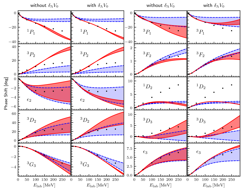
Figure 3: The results of the leading-order (blue dashed lines) and next-to-leading-order (red solid lines) calculations with the local regulator for selected $P$- and $D$-wave phase shifts. The bands indicate the variation of the one-pion-exchange cutoff within the range $\Lambda_{1\pi}\in(300,800)$ MeV. The right columns correspond to the NLO potential with the regulator correction $\delta_{\Lambda}V_{0}$, while the results in the left columns are obtained without this term. The plots were created using Matplotlib Hunter (2007).

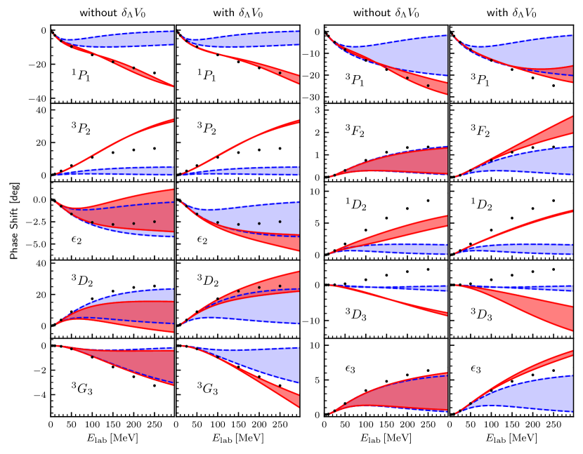
Figure 4: The results of the leading-order (blue dashed lines) and next-to-leading-order (red solid lines) calculations with the non-local regulator for selected $P$- and $D$-wave phase shifts. The bands indicate the variation of the one-pion-exchange cutoff within the range $\Lambda_{1\pi}\in(300,800)$ MeV. The right columns correspond to the NLO potential with the regulator correction $\delta_{\Lambda}V_{0}$, while the results in the left columns are obtained without this term.

The results for the phase shifts of the LO and NLO calculations are presented in Figs. 3, 4. The bands correspond to the variation of the cutoff. Two versions of the NLO interactions are shown: the one that contains the regulator correction $\delta_{\Lambda}V_{0}$ and the one that does not. Our calculations are compared with the results of the Nijmegen partial wave analysis Stoks et al. (1993). For $P$-waves, we have fitted the leading contact interactions appearing at next-to-leading order to the Nijmegen phase shifts up to $E_{\text{lab}}=150$ MeV. The results for $D$-waves do not involve free parameters.

As one can see from the figures, the convergence pattern is reasonable in all studied partial waves if one considers the energy region $E_{\text{lab}}\lesssim 150$ MeV or $p_{\text{on}}\lesssim 260$ MeV. If one aims at constructing an efficient scheme at higher energies (where the expansion parameter gets larger), the natural procedure would be to promote the $P$-wave contact interactions to leading order (e.g. in the ${}^{1}P_{1}$ and ${}^{3}P_{2}$ waves) and some $D$-wave contact terms to next-to-leading order (e.g. in the ${}^{3}D_{2}$ wave) in order to prevent possible issues with a large violation of unitarity within the schemes that rely on a perturbative treatment of subleading terms.

Looking at the cutoff dependence of our NLO results, one indeed observes that the corresponding bands, in most cases, become narrower upon explicitly including the $\delta_{\Lambda}V_{0}$ correction. One noticeable exception is the ${}^{3}F_{2}$ partial wave with the local regulator. However, a comparison to the results obtained using a nonlocal regulator suggests that the small band in calculations without the $\delta_{\Lambda}V_{0}$ correction is accidental. Notice further that the phase shift in the ${}^{3}F_{2}$ partial wave is several times smaller than in the other $F$-waves, and the resulting band width is still considerably smaller compared to the leading short-range contribution in that channel Reinert et al. (2018). Another exception is the ${}^{3}D_{3}$ partial wave with the non-local regulator. In this case, we again observe large cancellations for the NLO amplitude without $\delta_{\Lambda}V_{0}$. Notice that the boundaries of the shown band correspond to the limiting values of the cutoffs ($300$ and $800$ MeV), whereas for the intermediate values, the curves go slightly outside of the band (and are not shown). This partial wave is known to suffer from a very slow convergence of the EFT expansion due to the negligibly small contribution of the unregularized one-pion-exchange potential. Finally, one observes that the bands for the NLO results with $\delta_{\Lambda}V_{0}$ become particularly narrow for the ${}^{1}D_{2}$, ${}^{3}G_{3}$, $\epsilon_{3}$ partial waves, which is an indication that the LO interaction in those partial waves is purely perturbative.

In general, one expects that the cutoff dependence will be further reduced upon inclusion of higher-order corrections in $\delta_{\Lambda}V_{0}$.

VI Summary and outlook

We have analyzed the nucleon-nucleon interaction in chiral effective theory with a finite cutoff, i.e., a cutoff of the order of the hard scale. We have formulated a scheme based on the chiral effective Lagrangian that allows one to take into account the leading-order interaction non-perturbatively and to perform a perturbative expansion in terms of the subleading interactions. The dependence of the theory on the cutoff is also eliminated perturbatively, order by order, without changing a non-perturbative regime. This scheme ensures that the basic principles of EFT are met on the formal level: the constructed $S$-matrix is most general and satisfies analyticity, perturbative unitarity and a power counting, and the symmetries of the underlying theory are maintained.

The main question we addressed in this study is whether the power counting is still satisfied for the renormalized amplitude within our scheme. Renormalization of the scattering amplitude is necessary not only because of divergent loop integrals, but also due to the presence of positive powers of the (finite) cutoff that violate the naive power counting. We have shown that in the $S$-wave nucleon-nucleon amplitudes, one can absorb the power-counting breaking terms at all orders in the LO interaction by a renormalization of the leading order contact interactions as long as the cutoff is chosen to be of the order of the hard scale. In order to prove this statement, we have implemented the BPHZ subtraction procedure. A suitable sector decomposition of the multiple momentum integrals, combined with the rotation of the integration contour into the complex plain, allowed us to impose the relevant bounds on the considered amplitudes. For higher partial waves, we have demonstrated that no power-counting breaking terms appear at any order in the LO interaction. These results have been obtained for a rather general class of local and non-local regulators. The renormalizability has been proven at NLO to all orders in the LO interaction (but not for the purely non-perturbative case).

In order to illustrate how this scheme works in practice, we have calculated the next-to-leading-order nucleon-nucleon amplitude for the $P$- and $D$-waves, where the leading order interaction can be regarded as being sufficiently perturbative, i.e. one can numerically reproduce the full result with a finite number of iterations. In the $P$-waves, the contact terms quadratic in momenta have been fitted to the result of the Nijmegen partial-wave analysis, whereas the $D$-wave amplitudes are parameter-free. The resulting phase shifts are shown in Figs. 3 and 4 up to the laboratory energy of $E_{\text{lab}}=300$ MeV. We have also analyzed perturbative corrections due to the finite-cutoff artifacts. As expected, we found that their explicit inclusion allows one to significantly reduce the residual cutoff dependence in most cases, especially when the local form of the regulator is used.

As the next step, based on the findings of the present paper, we are going to consider the situation when the leading order interaction is essentially non-perturbative and the LO amplitude cannot be reproduced by a finite number of iterations. It is also important to extend the scheme to higher chiral orders and to reactions involving electroweak currents. Last but not least, it would also be interesting to apply our method to few-nucleon systems, in particular, regulated on the lattice.

Appendix A Bounds for real and complex momenta

The components of the initial and final nucleon c.m. momenta $p$ and $p^{\prime}$ are given by

$$\vec{p}=p\begin{pmatrix}0\\ 0\\ 1\end{pmatrix}\,,\quad\vec{p}\,^{\prime}=p^{\prime}\begin{pmatrix}\sin\theta\cos\phi\\ \sin\theta\sin\phi\\ \cos\theta\end{pmatrix}\,,$$ (150)

where $p$ is either $p=p_{\text{on}}$ or lies on the complex contour $p\in\mathcal{C}$: $p=|p|\exp(-i\alpha_{\mathcal{C}})$, and $p^{\prime}$ is either $p^{\prime}=p_{\text{on}}$ or $p^{\prime}=|p^{\prime}|\exp(-i\alpha_{\mathcal{C}})$.

The following obvious inequalities for $\vec{q}=\vec{p}\,^{\prime}-\vec{p}$ and $\vec{k}=(\vec{p}\,^{\prime}+\vec{p})/2$ hold:

$$|q_{i}|\leq|p|+|p^{\prime}|\,,\quad|q_{i}q_{j}|\leq 2(|p|^{2}+|p^{\prime}|^{2})\,,\quad|q^{2}|\leq 2(|p|^{2}+|p^{\prime}|^{2})\,,$$ (151)

and

$$|k_{i}|\leq\frac{1}{2}(|p|+|p^{\prime}|)\,,\quad|k_{i}k_{j}|\leq\frac{1}{2}(|p|^{2}+|p^{\prime}|^{2})\,,\quad|k_{i}q_{j}|\leq|p|^{2}+|p^{\prime}|^{2}\,,\quad|k^{2}|\leq\frac{1}{2}(|p|^{2}+|p^{\prime}|^{2})\,.$$ (152)

Appendix B Bounds on the typical denominator

Below, we obtain bounds for the typical denominator

$$q^{2}+\mu^{2}=p^{\prime 2}+p^{2}-2pp^{\prime}x+\mu^{2}\,,$$ (153)

with $\mu\geq M_{\pi}$.

It is convenient to provide unified bounds for all considered momenta $p$ and $p^{\prime}$ regardless of whether they are real and on shell or lie on the complex contour. The following estimates will be proven:

$$\big{|}q^{2}+\mu^{2}\big{|}\geq\mathcal{M}_{\text{den},1}\left(\sum_{i=1}^{3}|q_{i}|^{2}+\mu^{2}\right)\geq\mathcal{M}_{\text{den},1}\big{(}|q|^{2}+\mu^{2}\big{)}\,,$$ (154)

$$\big{|}q^{2}+\mu^{2}\big{|}\geq\mathcal{M}_{\text{den},2}\big{(}|p|^{2}+|p^{\prime}|^{2}-2|p||p^{\prime}|x+\mu^{2}\big{)}\geq\mathcal{M}_{\text{den},2}\big{[}(|p|^{\prime}-|p|)^{2}+\mu^{2}\big{]}\,.$$ (155)

When both momenta $p$ and $p^{\prime}$ are on shell, $\mathcal{M}_{\text{den},1}=\mathcal{M}_{\text{den},2}=1$. When both momenta $p$ and $p^{\prime}$ lie on the complex contour $p,\,p^{\prime}\in\mathcal{C}$, $\mathcal{M}_{\text{den},1}=\mathcal{M}_{\text{den},2}=\cos(\alpha_{\mathcal{C}})$:

$$|q^{2}+\mu^{2}|=|e^{-2i\alpha_{\mathcal{C}}}|q^{2}|+\mu^{2}|=|e^{-i\alpha_{\mathcal{C}}}|q^{2}|+e^{i\alpha_{\mathcal{C}}}\mu^{2}|>\Re(e^{-i\alpha_{\mathcal{C}}}|q^{2}|+e^{i\alpha_{\mathcal{C}}}\mu^{2})=\cos(\alpha_{\mathcal{C}})(|q^{2}|+\mu^{2})\,.$$ (156)

Now, we prove Eq. (154) for the configuration when $p=p_{\text{on}}$ and $p^{\prime}\in\mathcal{C}$.

The real part of $q^{2}$ satisfies:

$$\Re(q^{2}) = |p^{\prime}|^{2}\cos(2\alpha_{\mathcal{C}})+p_{\text{on}}^{2}-2|p^{\prime}|p_{\text{on}}x\cos(\alpha_{\mathcal{C}})>-\mathcal{M}_{\alpha_{\mathcal{C}},1}M_{\pi}^{2}\,,$$

$$\mathcal{M}_{\alpha_{\mathcal{C}},1} = \frac{1}{4}[1-\tan^{2}(\alpha_{\mathcal{C}})]\approx\frac{1}{4}\,,$$ (157)

where we have used that $p_{\text{on}}<\frac{M_{\pi}}{\tan(2\alpha_{\mathcal{C}})}$ . It follows then:

$$|q^{2}+\mu^{2}| > \Re(q^{2}+\mu^{2})>M_{\mu}\mu^{2}\,,$$

$$M_{\mu} = 1-\mathcal{M}_{\alpha_{\mathcal{C}},1}\frac{M^{2}}{\mu^{2}}\,.$$ (158)

On the other hand,

$$|q^{2}+\mu^{2}| = ||p^{\prime}|^{2}-2|p^{\prime}|p_{\text{on}}xe^{i\alpha_{\mathcal{C}}}+e^{2i\alpha_{\mathcal{C}}}(p_{\text{on}}^{2}+\mu^{2})|$$ (159)

$$> \Re(|p^{\prime}|^{2}-2|p^{\prime}|p_{\text{on}}xe^{i\alpha_{\mathcal{C}}}+e^{2i\alpha_{\mathcal{C}}}(p_{\text{on}}^{2}+\mu^{2}))$$

$$= |p^{\prime}|^{2}-2|p^{\prime}|p_{\text{on}}x\cos(\alpha_{\mathcal{C}})+\cos(2\alpha_{\mathcal{C}})(p_{\text{on}}^{2}+\mu^{2})$$

$$> |p^{\prime}|^{2}+p_{\text{on}}^{2}-2|p^{\prime}|p_{\text{on}}x\cos(\alpha_{\mathcal{C}})+\mathcal{M}_{\alpha_{\mathcal{C}},2}M_{\pi}^{2}$$

$$> |p^{\prime}|^{2}+p_{\text{on}}^{2}-2|p^{\prime}|p_{\text{on}}x\cos(\alpha_{\mathcal{C}})\,,$$

$$\mathcal{M}_{\alpha_{\mathcal{C}},2} = \cos(2\alpha_{\mathcal{C}})+\cot^{2}(2\alpha_{\mathcal{C}})[\cos(2\alpha_{\mathcal{C}})-1]=1-\frac{1}{2\cos^{2}(\alpha_{\mathcal{C}})}\approx\frac{1}{2}\,.$$

We can rewrite Eq. (159) as

$$|q^{2}+\mu^{2}|>|p^{\prime}|^{2}(1-x^{2})+|p_{\text{on}}-p^{\prime}x|^{2}=\sum_{i}|q_{i}|^{2}\,.$$ (160)

Combining Eq. (158) and Eq. (160), we obtain the bound (154):

$$|q^{2}+\mu^{2}|\geq\mathcal{M}_{\text{den},1}\left(\sum_{i}|q_{i}|^{2}+\mu^{2}\right)\,,\quad\mathcal{M}_{\text{den},1}=\frac{1-\mathcal{M}_{\alpha_{\mathcal{C}},1}}{2-\mathcal{M}_{\alpha_{\mathcal{C}},1}}<\frac{M_{\mu}}{M_{\mu}+1}\,.$$ (161)

From Eq. (159), we can also deduce

$$|q^{2}+\mu^{2}|>\cos(\alpha_{\mathcal{C}})\left(|p^{\prime}|^{2}+p_{\text{on}}^{2}-2p_{\text{on}}|p^{\prime}|x\right)\,.$$ (162)

Combining Eq. (158) and Eq. (162), we obtain the bound (155):

$$|q^{2}+\mu^{2}| \geq \mathcal{M}_{\text{den},2}(|p^{\prime}|^{2}+p_{\text{on}}^{2}-2|p^{\prime}|p_{\text{on}}x+\mu^{2})\,,$$

$$\mathcal{M}_{\text{den},2} = \cos(\alpha_{\mathcal{C}})\frac{1-\mathcal{M}_{\alpha_{\mathcal{C}},1}}{1+\cos(\alpha_{\mathcal{C}})-\mathcal{M}_{\alpha_{\mathcal{C}},1}}<\frac{M_{\mu}\cos(\alpha_{\mathcal{C}})}{M_{\mu}+\cos(\alpha_{\mathcal{C}})}\,.$$ (163)

Equations. (161), (163) can be combined with the cases $p=p^{\prime}=p_{\text{on}}$ and $p\,,p^{\prime}\in\mathcal{C}$ to arrive at Eqs. (154), (155). It is important to emphasize that $\mathcal{M}_{\text{den},1}$ and $\mathcal{M}_{\text{den},2}$ do not depend on $\mu$.

From Eqs. (154), (155), it follows:

$$\left|\frac{q_{i}q_{j}}{q^{2}+\mu^{2}}\right|<\mathcal{M}_{\text{den},1}^{-1}\,,\quad\left|\frac{q^{2}}{q^{2}+\mu^{2}}\right|<\mathcal{M}_{\text{den},1}^{-1}\,,\quad i,j=1,2,3\,,$$ (164)

and

$$\left|\frac{(\vec{k}\times\vec{q})_{i}}{q^{2}+\mu^{2}}\right| = \left|\frac{(\vec{p}\times\vec{p}\,^{\prime})_{i}}{q^{2}+\mu^{2}}\right|\leq\mathcal{M}_{\text{den},2}^{-1}\frac{|p||p^{\prime}|\sqrt{1-x^{2}}}{|p|^{2}+|p^{\prime}|^{2}-2|p||p^{\prime}|x+\mu^{2}}=\mathcal{M}_{\text{den},2}^{-1}\frac{|p||p^{\prime}|\sqrt{1-x^{2}}}{\left(|p|-|p^{\prime}|\right)^{2}+2|p||p^{\prime}|(1-x)+\mu^{2}}$$ (165)

$$\leq \mathcal{M}_{\text{den},2}^{-1}\frac{|p||p^{\prime}|\sqrt{1-x^{2}}}{|p||p^{\prime}|(1-x^{2})+\mu^{2}}\leq\mathcal{M}_{\text{den},2}^{-1}\left(1-x^{2}\right)^{-1/2}\,,\quad i=1,2,3\,.$$

Appendix C Bounds for subtractions

In this section, we provide bounds for the remainders $\Delta_{p}^{(n)}$, $\Delta_{p^{\prime}}^{(n)}$ for various functions relevant for our study.

We define the subtraction remainders for a function $f(p^{\prime},p)$ as:

$$\Delta_{p}^{(n)}f(p^{\prime},p) = f(p^{\prime},p)-\sum_{i=0}^{n}\frac{\partial^{i}f(p^{\prime},p)}{i!(\partial p)^{i}}\bigg{|}_{p=0}p^{i}\,,$$

$$\Delta_{p^{\prime}}^{(n)}f(p^{\prime},p) = f(p^{\prime},p)-\sum_{i=0}^{n}\frac{\partial^{i}f(p^{\prime},p)}{i!(\partial p^{\prime})^{i}}\bigg{|}_{p^{\prime}=0}(p^{\prime})^{i}\,,$$

$$\Delta_{p}f(p^{\prime},p) \equiv \Delta_{p}^{(0)}f(p^{\prime},p)\,,$$

$$\Delta_{p^{\prime}}f(p^{\prime},p) \equiv \Delta_{p^{\prime}}^{(0)}f(p^{\prime},p)\,.$$ (166)

For a product of two functions $f_{1}(p)f_{2}(p)$, it is convenient to utilize the identities:

$$\Delta_{p}\left(f_{1}(p)f_{2}(p)\right) = f_{1}(p)\Delta_{p}f_{2}(p)+\Delta_{p}f_{1}(p)f_{2}(0)\,,$$

$$\Delta^{(n)}_{p}\left(f_{1}(p)f_{2}(p)\right) = f_{1}(p)\Delta^{(n)}_{p}f_{2}(p)+\sum_{i=0}^{n}\Delta^{(n-i)}_{p}f_{1}(p)\frac{f_{2}^{(i)}(0)}{i!}p^{i}$$

$$= f_{1}(p)\Delta^{(n)}_{p}f_{2}(p)+\Delta^{(n)}_{p}f_{1}(p)f_{2}(p)$$

$$+ \sum_{i=1}^{n}\Delta^{(n-i)}_{p}f_{1}(p)\Delta^{(i-1)}_{p}f_{2}(p)-\sum_{i=0}^{n}\Delta^{(n-i)}_{p}f_{1}(p)\Delta^{(i)}_{p}f_{2}(p)\,.$$ (168)

C.1 Polynomials in momenta

Consider a homogeneous polynomial $Q_{m}(p^{\prime},p)$:

$$Q_{m}(p^{\prime},p)=\sum_{\alpha,\beta}\mathcal{M}_{\alpha\beta}p^{\alpha}p^{\prime\beta}\,,\quad\alpha+\beta=m\,,$$ (169)

e.g., $q^{2}$, $q_{i}q_{j}q^{2}$, $\vec{q}\times\vec{k}$, etc. Since $Q_{m}(p^{\prime},p)$ is a polynomial in $p$ and $p^{\prime}$, the following inequalities for the residues hold:

$$\left|\Delta_{p}^{(n)}Q_{m}(p^{\prime},p)\right|\;\leq\;\mathcal{M}_{Q}^{m,n}|p^{\prime}|^{m-n-1}|p|^{n+1}\;=\;\mathcal{M}_{Q}^{m,n}\left|\frac{p}{p^{\prime}}\right|^{n+1}|p^{\prime}|^{m}\,,\quad\text{ if }|p^{\prime}|>|p|\,,$$ (170)

and symmetrically for $\Delta_{p^{\prime}}^{(n)}Q_{m}(p^{\prime},p)$.

The derivatives of $Q_{m}(p^{\prime},p)$ are bounded by (including the case $n=0$)

$$p^{n}\frac{\partial^{n}Q_{m}(p^{\prime},p)}{(\partial p)^{n}}\bigg{|}_{p=0}\leq\mathcal{M}_{\partial Q}^{m,n}\left|\frac{p}{p^{\prime}}\right|^{n}|p^{\prime}|^{m}\,,$$ (171)

and symmetrically for $p\leftrightarrow p^{\prime}$.

C.2 Non-local form factor

For a non-local form factor of the form

$$F_{\Lambda,m}(p^{\prime},p)=F_{\Lambda,m}(p^{\prime})F_{\Lambda,m}(p)\,,\quad F_{\Lambda,m}(p)=\left(\frac{\Lambda^{2}}{p^{2}+\Lambda^{2}}\right)^{m}\,,$$ (172)

the remainders $\Delta_{p}^{(n)}$ can be represented as

$$\Delta_{p}^{(n)}F_{\Lambda,m}(p^{\prime},p)=\left(\frac{\Lambda^{2}}{p^{\prime 2}+\Lambda^{2}}\frac{\Lambda^{2}}{p^{2}+\Lambda^{2}}\right)^{m}\frac{p^{n+1}\sum_{\alpha+\beta=2m+n-1}\mathcal{M}_{\alpha\beta}p^{\alpha}\Lambda^{\beta}}{\Lambda^{2(n+m)}}\,.$$ (173)

Using the inequalities

$$|p^{2}+\Lambda^{2}|>|p|^{2}\,,\quad|p^{2}+\Lambda^{2}|\geq\Lambda^{2}\,,$$ (174)

the remainders can be bounded as

$$\left|\Delta_{p}^{(n)}F_{\Lambda,m}(p^{\prime},p)\right| \leq \mathcal{M}_{F}^{m,n}\left|\frac{p}{\Lambda}\right|^{n+1}\left|F_{\Lambda,m}(p^{\prime})F_{\Lambda,m}(p)\right|$$ (175)

$$\leq \mathcal{M}_{F}^{m,n}\left|\frac{p}{p^{\prime}}\right|^{n+1}\left|F_{\Lambda,m-\frac{n+1}{2}}(p^{\prime})\right|\,,\quad\text{ if }|p^{\prime}|>|p|\,.$$

The derivatives of $F_{\Lambda,m}(p^{\prime},p)$ satisfy the following inequalities:

$$\left|p^{n}\frac{\partial^{n}F_{\Lambda,m}(p^{\prime},p)}{(\partial p)^{n}}\bigg{|}_{p=0}\right|\leq\mathcal{M}_{\partial F}^{m,n}\left|\frac{p}{p^{\prime}}\right|^{n}\left|F_{\Lambda,m-\frac{n+1}{2}}(p^{\prime})\right|\,,$$ (176)

including the case $n=0$.

From Eqs. (175), (170), (171) and the identity for the remainder of a product (C), the following bound can be imposed for a function $\Phi_{k,m}(p^{\prime},p)=Q_{k}(p^{\prime},p)F_{\Lambda,m}(p^{\prime},p)$, where $Q_{k}(p^{\prime},p)$ is an arbitrary homogeneous polynomial of degree $k$:

$$\left|\Delta_{p}^{(n)}\Phi_{k,m}(p^{\prime},p)\right|\leq\mathcal{M}_{\Phi}^{k,m,n}\left|\frac{p}{p^{\prime}}\right|^{n+1}|p^{\prime}|^{k}\left|F_{\Lambda,m-\frac{n+1}{2}}(p^{\prime})\right|\,,\quad\text{ if }|p^{\prime}|>|p|\,,$$ (177)

and for the derivatives of $\Phi_{k,m}$:

$$\left|p^{n}\frac{\partial^{n}\Phi_{k,m}(p^{\prime},p)}{(\partial p)^{n}}\bigg{|}_{p=0}\right|\leq\mathcal{M}_{\partial\Phi}^{m,n}\left|\frac{p}{p^{\prime}}\right|^{n}|p^{\prime}|^{k}\left|F_{\Lambda,m-\frac{n+1}{2}}(p^{\prime})\right|\,,$$ (178)

including the case $n=0$. All inequalities of this subsection hold also under interchange $p\leftrightarrow p^{\prime}$.

C.3 Local form factor

In the case of a local regulator, a typical function $f_{\mu}(p^{\prime},p)$

$$f_{\mu}(p^{\prime},p)=\frac{1}{q^{2}+\mu^{2}}=\frac{1}{p^{2}+p^{\prime 2}-2pp^{\prime}x+\mu^{2}}\,,\quad-1\leq x\leq 1\,,$$ (179)

appears in the one-pion-exchange and two-pion-exchange potentials. Its subtraction remainders are bounded as

$$\left|\Delta_{p}^{(n)}f_{\mu}(p^{\prime},p)\right|\leq\mathcal{M}_{f,n}\left|\frac{p}{p^{\prime}}\right|^{n+1}\left|f_{\mu}(p^{\prime},p)\right|\,,\quad\text{ if }|p^{\prime}|>|p|\,.$$ (180)

Proof: The remainder $\Delta_{p}^{(n)}$ can be represented as

$$\Delta_{p}^{(n)}f_{\mu}(p^{\prime},p)=\frac{p^{n+1}Q_{n+1}(p,p^{\prime},\mu^{2})}{(p^{2}+p^{\prime 2}-2pp^{\prime}x+\mu^{2})(p^{\prime 2}+\mu^{2})^{n+1}}\,,$$ (181)

where $Q_{n+1}$ is a homogeneous polynomial

$$Q_{n+1}(p,p^{\prime},\mu^{2})=\sum_{\alpha\beta\gamma}\mathcal{M}_{\alpha\beta\gamma}p^{\prime\alpha}p^{\beta}\mu^{\gamma}\,,\quad\alpha+\beta+\gamma=n+1\,.$$ (182)

For $|p^{\prime}|>|p|$, we get:

$$\left|\frac{\mu}{(p^{\prime 2}+\mu^{2})^{1/2}}\right|<1\,,\quad\left|\frac{p}{(p^{\prime 2}+\mu^{2})^{1/2}}\right|<\left|\frac{p^{\prime}}{(p^{\prime 2}+\mu^{2})^{1/2}}\right|<1\,,$$

and, therefore

$$\left|\frac{p^{\prime\alpha}p^{\beta}\mu^{\gamma}}{(p^{\prime 2}+\mu^{2})^{(n+1)}}\right| \leq \frac{1}{|p^{\prime}|^{n+1}}\,,$$

$$\left|\Delta_{p}^{(n)}f_{\mu}(p^{\prime},p)\right| \leq \left|\frac{p}{p^{\prime}}\right|^{n+1}\left|f_{\mu}(p^{\prime},p)\right|\sum_{\alpha\beta\gamma}|\mathcal{M}_{\alpha\beta\gamma}|\,,$$ (184)

which completes the proof. Note that coefficients $\mathcal{M}_{f,n}$ are independent of $\mu$.

For the derivatives $\frac{\partial^{n}f_{\mu}(p^{\prime},p)}{(\partial p)^{n}}$, we obtain

$$\left|p^{n}\frac{\partial^{n}f_{\mu}(p^{\prime},p)}{(\partial p)^{n}}\bigg{|}_{p=0}\right| = \left|p^{n}\frac{\sum_{\alpha+\beta=n}\mathcal{M}_{n,\alpha\beta}p^{\prime\alpha}\mu^{\beta}}{(p^{\prime 2}+\mu^{2})^{n+1}}\right|$$ (185)

$$\leq \sum_{\alpha+\beta=n}|\mathcal{M}_{n,\alpha\beta}||f_{\mu}(p^{\prime},0)|\left|\frac{p}{p^{\prime}}\right|^{n}$$

$$= \mathcal{M}_{\partial f,n}|f_{\mu}(p^{\prime},0)|\left|\frac{p}{p^{\prime}}\right|^{n}\,.$$

From the product formula (168), it follows that the same constraints as in Eq. (180) and in Eq. (185) hold for a product of two (or more) functions $f_{\mu_{i}}(p^{\prime},p)$

$$f_{\{\mu_{i}\}}(p^{\prime},p)=\prod_{i=1,k}f_{\mu_{i}}(p^{\prime},p)$$ (186)

and for any positive integer power of $f_{\mu}(p^{\prime},p)$.

For a function $\psi_{k,\{\mu_{i}\}}(p^{\prime},p)=Q_{k}(p^{\prime},p)f_{\{\mu_{i}\}}(p^{\prime},p)$, which is a product of several local structures $f_{\mu_{i}}(p^{\prime},p)$ and a homogeneous polynomial $Q_{k}(p^{\prime},p)$, the following bounds can be obtained:

$$\left|\Delta_{p}^{(n)}\psi_{k,\{\mu_{i}\}}(p^{\prime},p)\right|\leq\mathcal{M}_{\psi}^{k,n}\left|\frac{p}{p^{\prime}}\right|^{n+1}\left(|\psi_{k,\{\mu_{i}\}}(p^{\prime},p)|+\left|p^{\prime k}f_{\{\mu_{i}\}}(p^{\prime},0)\right|\right)\,,\quad\text{ if }|p^{\prime}|>|p|\,,$$ (187)

$$\left|p^{n}\frac{\partial^{n}\psi_{k,\{\mu_{i}\}}(p^{\prime},p)}{(\partial p)^{n}}\bigg{|}_{p=0}\right|\leq\mathcal{M}_{\partial\psi}^{k,n}\left|p^{\prime k}f_{\{\mu_{i}\}}(p^{\prime},0)\right|\left|\frac{p}{p^{\prime}}\right|^{n}\,,\quad n\geq 0\,.$$ (188)

They can be readily derived from the product formula (C) and Eqs. (177), (178), (180), (185).

Finally, from the product formula (C) and Eqs. (170), (171), (180), (185), for a function

$$\Psi_{k,m,\{\mu_{i}\}}(p^{\prime},p)=Q_{k}(p^{\prime},p)F_{\Lambda,m}(p^{\prime},p)f_{\{\mu_{i}\}}(p^{\prime},p)\,,$$ (189)

the following bounds hold:

$$\left|\Delta_{p}^{(n)}\Psi_{k,m,\{\mu_{i}\}}(p^{\prime},p)\right|\leq\mathcal{M}_{\Psi}^{k,n}\left|\frac{p}{p^{\prime}}\right|^{n+1}\Big{(}|\Psi_{k,m,\{\mu_{i}\}}(p^{\prime},p)|+\left|p^{\prime k}F_{\Lambda,m-\frac{n+1}{2}}(p^{\prime})f_{\{\mu_{i}\}}(p^{\prime},0)\right|\Big{)}\,,\quad\text{ if }|p^{\prime}|>|p|\,,$$ (190)

$$\left|p^{n}\frac{\partial^{n}\Psi_{k,m,\{\mu_{i}\}}(p^{\prime},p)}{(\partial p)^{n}}\bigg{|}_{p=0}\right|\leq\mathcal{M}_{\partial\Psi}^{k,n}\left|p^{\prime k}F_{\Lambda,m-\frac{n+1}{2}}(p^{\prime})f_{\{\mu_{i}\}}(p^{\prime},0)\right|\left|\frac{p}{p^{\prime}}\right|^{n}\,,\quad n\geq 0\,.$$ (191)

The classes of functions $\Phi_{k,m}(p^{\prime},p)$, $\psi_{k,\{\mu_{i}\}}(p^{\prime},p)$ and $\Psi_{k,m,\{\mu_{i}\}}(p^{\prime},p)$ cover all structures that are relevant for our study.

Notice further that all inequalities of this subsection hold also under the interchange $p\leftrightarrow p^{\prime}$.

C.4 Gaussian form factors

The bounds for Gaussian local and non-local regulators and their subtraction remainders and derivatives can be reduced to the power-law regulators with an arbitrary power $m$. In order to show this, we will use the properties of the exponential function described below.

Since the function $\exp\left(-z^{2}\right)$ decreases at infinity for $\Re(z^{2})>0$ faster than any power of $z$, we can write:

$$\left|\exp\left(-z^{2}\right)z^{n}\right|=\exp\left[-\Re(z^{2})\right]|z|^{n}\leq\mathcal{M}_{\text{exp},n}\,,$$ (192)

where we assume that $\arg(z)=0$ or $\arg(z)=-\alpha_{\mathcal{C}}$.

The derivatives of the function $\exp\left(-z^{2}\right)$ are bounded by

$$\left|\frac{\operatorname{d}^{n}\exp\left(-z^{2}\right)}{\operatorname{d}z^{n}}\bigg{|}_{z=0}\right|\leq\mathcal{M}_{\text{exp},d,n}\,.$$ (193)

The remainder of the function $\exp\xi$,

$$\Delta_{\text{exp}}^{(n)}(\xi)\equiv\Delta_{\xi}^{(n)}\exp\xi=\exp\xi-\sum_{i=0}^{n}\frac{\xi^{n}}{n!}\,,$$ (194)

obey the following constraints:

$$\left|\Delta_{\xi}^{(n)}\exp\left(\xi\right)\right|\leq\frac{|\xi|^{n+1}}{(n+1)!}\,,\quad\text{ for }\Re(\xi)\leq 0\,,$$

$$\left|\Delta_{\xi}^{(n)}\exp\left(\xi\right)\right|\leq\frac{|\xi|^{n+1}}{(n+1)!}\exp\left[\Re(\xi)\right]\,,\quad\text{ for }\Re(\xi)>0\,,$$ (195)

which can be proven by induction using the recurrence relation

$$\Delta_{\text{exp}}^{(n+1)}(\xi)=\xi\int_{0}^{1}\Delta_{\text{exp}}^{(n)}(\tau\,\xi)d\tau\,.$$ (196)

C.5 Non-local Gaussian form factor

The case of the non-local Gaussian form factor

$$F_{\Lambda,\text{exp}}(p^{\prime},p)=F_{\Lambda,\text{exp}}(p^{\prime})F_{\Lambda,\text{exp}}(p)=\exp\left[-\left(p^{2}+p^{\prime 2}\right)/\Lambda^{2}\right]$$ (197)

can be reduced to the case of the non-local power-law form factor with an arbitrary power $m$ as will be shown below.

From Eqs. (192), (193), we can deduce the following inequalities for $F_{\Lambda,\text{exp}}(p^{\prime},p)$ and its derivatives:

$$\left|F_{\Lambda,\text{exp}}(p^{\prime},p)\right|\leq\mathcal{M}_{\text{exp},m}\left|\frac{\Lambda^{2}}{p^{2}+\Lambda^{2}}\right|^{m}\left|\frac{\Lambda^{2}}{p^{\prime 2}+\Lambda^{2}}\right|^{m}=\mathcal{M}_{\text{exp},m}\left|F_{\Lambda,m}(p^{\prime},p)\right|\,,$$ (198)

and

$$\left|p^{n}\frac{\partial^{n}F_{\Lambda,\text{exp}}(p^{\prime},p)}{{\partial p}^{n}}\bigg{|}_{p=0}\right|\leq\left|\exp\left(-p^{\prime}\,{}^{2}/\Lambda^{2}\right)\right|\left|\frac{p^{\prime}}{\Lambda}\right|^{n}\mathcal{M}_{\text{exp},d,n}\left|\frac{p}{p^{\prime}}\right|^{n}\leq\mathcal{M}_{\partial F,\text{exp}}^{m,n}\left|\frac{p}{p^{\prime}}\right|^{n}\left|F_{\Lambda,m-\frac{n+1}{2}}(p^{\prime})\right|\,,$$ (199)

and symmetrically for $p\leftrightarrow p^{\prime}$.

The remainders $\Delta_{p}^{(n)}F_{\Lambda,\text{exp}}(p^{\prime},p)$ can be bounded utilizing Eqs. (192), (195) as follows

$$\left|\Delta_{p}^{(n)}F_{\Lambda,\text{exp}}(p^{\prime},p)\right| \leq \frac{1}{[(n+1+\delta_{n})/2]!}\left|\frac{p}{\Lambda}\right|^{n+1+\delta_{n}}\left|\exp\left(-p^{\prime 2}/\Lambda^{2}\right)\right|$$ (200)

$$\leq \mathcal{M}_{F,\text{exp}}^{m,n}\left|\frac{p}{p^{\prime}}\right|^{n+1+\delta_{n}}\left|F_{\Lambda,m-\frac{n+1}{2}}(p^{\prime})\right|$$

$$\leq \mathcal{M}_{F,\text{exp}}^{m,n}\left|\frac{p}{p^{\prime}}\right|^{n+1}\left|F_{\Lambda,m-\frac{n+1}{2}}(p^{\prime})\right|\,,\quad\text{ if }|p^{\prime}|>|p|\,,$$

with $\delta_{n}=(n+1)\mod 2$ and, symmetrically, for $p\leftrightarrow p^{\prime}$.

Equations (198), (199), (200) are identical to Eqs. (172), (176), (175) for the non-local power-law form factors from the point of view of the upper bounds.

C.6 Local Gaussian form factor

The case of the local Gaussian form factor

$$F_{\Lambda,\text{exp}}(q)=\exp(-q^{2}/\Lambda^{2})=\exp\left[-\left(p^{2}+p^{\prime 2}-2pp^{\prime}x\right)/\Lambda^{2}\right]$$ (201)

can be reduced to the case of the local power-law form factor with an arbitrary power $m$ similarly to the non-local case. First, let us show that

$$\Re(q^{2})+\Lambda^{2}\geq\mathcal{M}_{\text{Re}}\left|q^{2}+\Lambda^{2}\right|\,.$$ (202)

If $p,p^{\prime}\in\mathcal{C}$, Eq. (202) holds with $\mathcal{M}_{\text{Re}}=\cos(2\alpha_{\mathcal{C}})$. If $p^{\prime}\in\mathcal{C}$ and $p=p_{\text{on}}$, we have (see Eq. (157)):

$$2\left|\Re(q^{2}+\Lambda^{2})\right|-\left|\Im(q^{2}+\Lambda^{2})\right| = 2|p^{\prime}|^{2}\cos(2\alpha_{\mathcal{C}})+2p_{\text{on}}^{2}-4|p^{\prime}|p_{\text{on}}x\cos(\alpha_{\mathcal{C}})+2\Lambda^{2}$$ (203)

$${}-s\left(|p^{\prime}|^{2}\sin(2\alpha_{\mathcal{C}})-2|p^{\prime}|p_{\text{on}}x\sin(\alpha_{\mathcal{C}})\right)$$

$$\geq -\frac{5p_{\text{on}}^{2}\sin^{2}(\alpha)}{2\cos(2\alpha)-s\sin(2\alpha)}+2\Lambda^{2}$$

$$\geq -M_{\pi}^{2}\frac{5\sin^{2}(\alpha)\cot^{2}(2\alpha)}{2\cos(2\alpha)-s\sin(2\alpha)}+2\Lambda^{2}$$

$$> 0\,,$$

where $s=\operatorname{sgn}\left[|p^{\prime}|^{2}\sin(2\alpha_{\mathcal{C}})-2|p^{\prime}|p_{\text{on}}x\sin(\alpha_{\mathcal{C}})\right]$. Therefore, Eq. (202) holds:

$$\left|\Re(q^{2}+\Lambda^{2})\right|\geq\frac{1}{3}\left(\left|\Re(q^{2}+\Lambda^{2})\right|+\left|\Im(q^{2}+\Lambda^{2})\right|\right)\geq\frac{1}{3}\left|q^{2}+\Lambda^{2}\right|\,.$$ (204)

From Eq. (202) and Eq. (192), we obtain the bound

$$\left|F_{\Lambda,\text{exp}}(q)\right|\leq\mathcal{M}_{\text{exp},q,m}\left|\frac{\Lambda^{2}}{q^{2}+\Lambda^{2}}\right|^{m}\,.$$ (205)

Since the derivative $\frac{\partial^{n}F_{\Lambda,\text{exp}}(q)}{{\partial p}^{n}}$ at $p=0$ is equal to

$$\frac{\partial^{n}F_{\Lambda,\text{exp}}(q)}{{\partial p}^{n}}\bigg{|}_{p=0}=F_{\Lambda,\text{exp}}(p^{\prime})P_{\partial,n}(p^{\prime}/\Lambda)/\Lambda^{n}\,,$$ (206)

where $P_{\partial,n}(z)$ is a polynomial of degree $n$, we can deduce from Eq. (192) the following bounds:

$$\left|p^{n}\frac{\partial^{n}F_{\Lambda,\text{exp}}(q)}{{\partial p}^{n}}\bigg{|}_{p=0}\right|\leq\mathcal{M}_{\partial F,\text{exp},q}^{m,n}\left|\frac{p}{p^{\prime}}\right|^{n}\left(\frac{\Lambda^{2}}{4|p^{\prime}|^{2}+\Lambda^{2}}\right)^{m}\leq\mathcal{M}_{\partial F,\text{exp},q}^{m,n}\left|\frac{p}{p^{\prime}}\right|^{n}\left|F_{\Lambda,m}(p^{\prime})\right|\,,$$ (207)

and

$$\left|p^{n}\frac{\partial^{n}F_{\Lambda,\text{exp}}(q)}{{\partial p}^{n}}\bigg{|}_{p=0}\right|\leq\mathcal{\tilde{M}}_{\partial F,\text{exp},q}^{(n)}\left|\frac{p}{p^{\prime}}\right|^{n}\frac{|p^{\prime}|^{2}}{\Lambda^{2}}\,,$$ (208)

including $n=0$.

Representing $F_{\Lambda,\text{exp}}(q)$ as

$$F_{\Lambda,\text{exp}}(q)=F_{\Lambda,\text{exp}}(p^{\prime},p)F_{\Lambda,pp^{\prime}}(p^{\prime},p)\,,\quad F_{\Lambda,pp^{\prime}}(p^{\prime},p)=\exp\left(2pp^{\prime}x/\Lambda^{2}\right)\,,$$ (209)

we can write down the remainders $\Delta_{p}^{(n)}F_{\Lambda,\text{exp}}(p^{\prime},p)$ using the product formula (C):

$$\Delta_{p}^{(n)}F_{\Lambda,\text{exp}}(q)=F_{\Lambda,pp^{\prime}}(p^{\prime},p)\Delta^{(n)}_{p}F_{\Lambda,\text{exp}}(p^{\prime},p)+\sum_{i=0}^{n}\Delta^{(n-i)}_{p}F_{\Lambda,pp^{\prime}}(p^{\prime},p)\frac{p^{i}}{i!}\frac{\partial^{i}F_{\Lambda,\text{exp}}(p^{\prime},p)}{{\partial p}^{i}}\bigg{|}_{p=0}\,.$$ (210)

The function $F_{\Lambda,pp^{\prime}}(p^{\prime},p)$ and the remainders $\Delta_{p}^{(n)}F_{\Lambda,pp^{\prime}}(p^{\prime},p)$ are bounded by (see Eq. (195))

$$\left|F_{\Lambda,pp^{\prime}}(p^{\prime},p)\right| \leq \exp\left[2\Re(pp^{\prime})/\Lambda^{2}\right]\,,$$

$$\left|\Delta_{p}^{(n)}F_{\Lambda,pp^{\prime}}(p^{\prime},p)\right| \leq \exp\left[2\Re(pp^{\prime})/\Lambda^{2}\right]\frac{|2pp^{\prime}|^{n+1}}{(n+1)!\Lambda^{2(n+1)}}\,.$$ (211)

From Eqs. (210), (211),  (199), (200), we obtain:

$$\left|\Delta_{p}^{(n)}F_{\Lambda,\text{exp}}(q)\right| \leq \exp-\left[\Re\left(p^{\prime}\,{}^{2}-2pp^{\prime}\right)/\Lambda^{2}\right]\left(\frac{1}{[(n+1+\delta_{n})/2]!}\left|\frac{p}{\Lambda}\right|^{n+1+\delta_{n}}+\left|\frac{p}{\Lambda}\right|^{n+1}\sum_{i=0}^{n}\left|\frac{p^{\prime}}{\Lambda}\right|^{n-i+1}\frac{\mathcal{M}_{\text{exp},d,n}}{(n-i+1)!i!}\right)$$ (212)

$$\leq \mathcal{M}_{\Delta}^{(m)}\exp\left[-\Re\left(p^{\prime}\,{}^{2}-2pp^{\prime}\right)/\Lambda^{2}\right]\left|\frac{p}{\Lambda}\right|^{n+1}\left(\left|\frac{p}{\Lambda}\right|^{\delta_{n}}+\left|\frac{p^{\prime}}{\Lambda}\right|P_{p^{\prime},n}\left(\left|\frac{p^{\prime}}{\Lambda}\right|\right)\right)\,,$$

where $\delta_{n}=\left[(n+1)\mod 2\right]$ and $P_{p^{\prime},n}$ is a polynomial of degree $n$ with non-negative coefficients.

Consider now the following three cases.

1. $|p|\leq\mathcal{M}_{pp^{\prime}}|p^{\prime}|$ ,
   where $\mathcal{M}_{pp^{\prime}}<1$ is some constant chosen such that

   $$\Re\left(p^{\prime 2}-2\mathcal{M}_{pp^{\prime}}pp^{\prime}|p^{\prime}|/|p|\right)\geq\mathcal{M}_{p^{\prime}}|p^{\prime}|^{2}\,.$$ (213)

   For example, for $\mathcal{M}_{pp^{\prime}}=1/4$, $\mathcal{M}_{p^{\prime}}=\cos(2\alpha)-\cos(\alpha)/2\gtrsim 1/4$ (assuming that $\alpha\leq\pi/8$, which corresponds to $\left(p_{\text{on}}\right)_{\text{max}}\geq M_{\pi}$).

   Then, Eq (212) becomes (after applying Eq. (192))

   $$\left|\Delta_{p}^{(n)}F_{\Lambda,\text{exp}}(q)\right| \leq \mathcal{M}_{\Delta}^{(m)}\exp\left(-\mathcal{M}_{p^{\prime}}|p^{\prime}|^{2}/\Lambda^{2}\right)\left|\frac{p}{\Lambda}\right|^{n+1}\left(\left|\frac{p^{\prime}}{\Lambda}\right|^{\delta_{n}}+\left|\frac{p^{\prime}}{\Lambda}\right|P_{p^{\prime},n}\left(\left|\frac{p^{\prime}}{\Lambda}\right|\right)\right)$$ (214)

   $$\leq \mathcal{M}_{F,q,1}^{m,n}\left|\frac{p}{p^{\prime}}\right|^{n+1}\left(\frac{\Lambda^{2}}{|p^{\prime}|^{2}(1+1/\mathcal{M}_{pp^{\prime}})^{2}+\Lambda^{2}}\right)^{m}$$

   $$\leq \mathcal{M}_{F,q,1}^{m,n}\left|\frac{p}{p^{\prime}}\right|^{n+1}\left|\frac{\Lambda^{2}}{q^{2}+\Lambda^{2}}\right|^{m}\,,$$

   where we have used that

   $$\left|q^{2}+\Lambda^{2}\right|\leq\left|q^{2}\right|+\Lambda^{2}\leq|p|^{2}+|p^{\prime}|^{2}+2|p||p^{\prime}|+\Lambda^{2}\leq|p^{\prime}|^{2}(1+1/\mathcal{M}_{pp^{\prime}})^{2}+\Lambda^{2}\,.$$ (215)

   An alternative constraint has the form

   $$\left|\Delta_{p}^{(n)}F_{\Lambda,\text{exp}}(q)\right|\leq\mathcal{\tilde{M}}_{F,q,1}^{(n)}\left|\frac{p}{p^{\prime}}\right|^{n+1}\frac{|p^{\prime}|^{2}}{\Lambda^{2}}\,,$$ (216)

   which is correct also for $n=0$ since $\delta_{0}=1$.

2. $\mathcal{M}_{pp^{\prime}}|p^{\prime}|\leq|p|\leq|p^{\prime}|\leq\Lambda$.

   Equation (212) yields

   $$\left|\Delta_{p}^{(n)}F_{\Lambda,\text{exp}}(q)\right| \leq \mathcal{M}_{\Delta}^{(m)}\exp(1)\left|\frac{p}{\Lambda}\right|^{n+1}\left(\left|\frac{p^{\prime}}{\Lambda}\right|^{\delta_{n}}+\left|\frac{p^{\prime}}{\Lambda}\right|P_{p^{\prime},n}\left(\left|\frac{p^{\prime}}{\Lambda}\right|\right)\right)$$ (217)

   $$\leq \frac{\mathcal{M}_{F,q,2}^{m,n}}{5^{m}}\left|\frac{p}{p^{\prime}}\right|^{n+1}$$

   $$\leq \mathcal{M}_{F,q,2}^{m,n}\left|\frac{p}{\Lambda}\right|^{n+1}\left|\frac{\Lambda^{2}}{q^{2}+\Lambda^{2}}\right|^{m}\,,$$

   where the last inequality follows from

   $$\left|q^{2}+\Lambda^{2}\right|\leq|p|^{2}+|p^{\prime}|^{2}+2|p||p^{\prime}|+\Lambda^{2}\leq 4|p^{\prime}|^{2}+\Lambda^{2}\leq 5\Lambda^{2}\,.$$ (218)

   Alternatively,

   $$\left|\Delta_{p}^{(n)}F_{\Lambda,\text{exp}}(q)\right|\leq\mathcal{\tilde{M}}_{F,q,2}^{(n)}\left|\frac{p}{\Lambda}\right|^{n+1}\frac{|p^{\prime}|^{2}}{\Lambda^{2}}\,.$$ (219)

3. $\mathcal{M}_{pp^{\prime}}|p^{\prime}|\leq|p|\leq\Lambda\leq|p^{\prime}|$.

Using the definition of the remainders (Eq. (166)) and Eqs. (205), (207)  (218), we get:

$$\left|\Delta_{p}^{(n)}F_{\Lambda,\text{exp}}(q)\right| \leq \left|F_{\Lambda,\text{exp}}(q)\right|+\sum_{i=0}^{n}\left|\frac{\partial^{i}F_{\Lambda,\text{exp}}(q)}{{\partial p}^{i}}\bigg{|}_{p=0}\right|\frac{|p|^{i}}{i!}$$ (220)

$$\leq \mathcal{M}_{\text{exp},q,m}\left|\frac{\Lambda^{2}}{q^{2}+\Lambda^{2}}\right|^{m}+\left(\frac{\Lambda^{2}}{4|p^{\prime}|^{2}+\Lambda^{2}}\right)^{m}\sum_{i=0}^{n}\frac{\mathcal{M}_{\partial F,\text{exp},q}^{(m,i)}}{i!}\left|\frac{p}{p^{\prime}}\right|^{i}$$

$$\leq \frac{\mathcal{M}_{\text{exp},q,m}}{\left(\mathcal{M}_{pp^{\prime}}\right)^{n+1}}\left|\frac{p}{p^{\prime}}\right|^{n+1}\left|\frac{\Lambda^{2}}{q^{2}+\Lambda^{2}}\right|^{m}+\left|\frac{p}{p^{\prime}}\right|^{n+1}\left|\frac{\Lambda^{2}}{q^{2}+\Lambda^{2}}\right|^{m}\sum_{i=0}^{n}\frac{\mathcal{M}_{\partial F,\text{exp},q}^{(m,i)}}{i!\left(\mathcal{M}_{pp^{\prime}}\right)^{n-i+1}}$$

$$\leq \mathcal{M}_{F,q,3}^{m,n}\left|\frac{p}{p^{\prime}}\right|^{n+1}\left|\frac{\Lambda^{2}}{q^{2}+\Lambda^{2}}\right|^{m}\,.$$

For $m=0$, it gives:

$$\left|\Delta_{p}^{(n)}F_{\Lambda,\text{exp}}(q)\right|\leq\mathcal{M}_{F,q,3}^{(n)}\left|\frac{p}{p^{\prime}}\right|^{n+1}\leq\mathcal{M}_{F,q,3}^{(n)}\left|\frac{p}{p^{\prime}}\right|^{n+1}\frac{|p^{\prime}|^{2}}{\Lambda^{2}}\,.$$ (221)

Combining all three cases, we obtain:

$$\left|\Delta_{p}^{(n)}F_{\Lambda,\text{exp}}(q)\right|\leq\mathcal{M}_{F,q}^{(n)}\left|\frac{p}{p^{\prime}}\right|^{n+1}\left|\frac{\Lambda^{2}}{q^{2}+\Lambda^{2}}\right|\,,\quad\text{ if }|p^{\prime}|>|p|\,,$$ (222)

or, alternatively,

$$\left|\Delta_{p}^{(n)}F_{\Lambda,\text{exp}}(q)\right|\leq\mathcal{\tilde{M}}_{F,q}^{(n)}\left|\frac{p}{p^{\prime}}\right|^{n+1}\frac{|p^{\prime}|^{2}}{\Lambda^{2}}\,,\quad\text{ if }|p^{\prime}|>|p|\,,$$ (223)

and, symmetrically, for $p\leftrightarrow p^{\prime}$.

Equations (205), (207), (222) are identical to Eqs. (179), (185), (180) for the local power-law form factors with $\mu=\Lambda$ and their generalizations for higher powers $m>1$ from the point of view of the upper bounds.

Appendix D Bounds on the plane-wave leading-order potential

In this section, we provide bounds for leading order potential. First, we consider the potential in the plane-wave basis. We treat all matrix elements of the spin and isospin matrices as constants of order one, and take care only of the dependence of the potential on the coupling constants, masses, cutoffs, momenta, and other scales.

The locally regularized one-pion exchange potential in the spin-triplet channel can be bounded using Eqs. (154),(155) by the following inequality:

$$\left|V^{(0)}_{1\pi,\text{t},\Lambda}(\vec{p}\,^{\prime},\vec{p})\right|\leq\left|\frac{g_{A}^{2}}{4F_{\pi}^{2}}\sum_{i,j}\mathcal{M}_{\text{t},ij}\frac{q_{i}q_{j}}{q^{2}+M_{\pi}^{2}}\frac{\Lambda_{\text{t},1}^{2}-M_{\pi}^{2}}{q^{2}+\Lambda_{\text{t},1}^{2}}\right|\leq\frac{2\pi\mathcal{M}_{\text{t}}}{m_{N}\Lambda_{V}}\frac{\Lambda^{2}}{(|p^{\prime}|-|p|)^{2}+\Lambda^{2}}=\frac{2\pi\mathcal{M}_{\text{t}}}{m_{N}\Lambda_{V}}F_{\Lambda}(|p^{\prime}|-|p|)\,,$$ (224)

where $\Lambda$ is the largest cutoff among all cutoffs used in the leading-order potential. For our estimates, it is sufficient to keep in the first inequality of Eq. (224) only one local form factor with the cutoff $\Lambda_{\text{t},1}$, which is the smallest among $\{\Lambda_{\text{t},i}\}$. The dimensionful factor $2\pi/m_{N}$ is introduced for convenience in order to identify the typical hard scale of the leading-order potential $\Lambda_{V}$. In particular, we treat the commonly used scale $\Lambda_{NN}=16\pi F_{\pi}^{2}/m_{N}/g_{A}^{2}$ as a quantity of order $\Lambda_{V}$.

If the triplet one-pion exchange potential is regularized by the non-local form factor, we obtain

$$\left|V^{(0)}_{1\pi,\text{t},\Lambda}(\vec{p}\,^{\prime},\vec{p})\right|\leq\left|\frac{g_{A}^{2}}{4F_{\pi}^{2}}\sum_{i,j}\mathcal{M}_{\text{t},ij}\frac{q_{i}q_{j}}{q^{2}+M_{\pi}^{2}}\frac{\Lambda^{2}}{p^{\prime 2}+\Lambda^{2}}\frac{\Lambda^{2}}{p^{2}+\Lambda^{2}}\right|\leq\frac{2\pi\mathcal{M}_{\text{t}}}{m_{N}\Lambda_{V}}\frac{\Lambda^{2}}{|p^{\prime}|^{2}+\Lambda^{2}}=\frac{2\pi\mathcal{M}_{\text{t}}}{m_{N}\Lambda_{V}}F_{\Lambda}(|p^{\prime}|)\,,$$ (225)

or, symmetrically,

$$\left|V^{(0)}_{1\pi,\text{t},\Lambda}(\vec{p}\,^{\prime},\vec{p})\right|\leq\frac{2\pi\mathcal{M}_{\text{t}}}{m_{N}\Lambda_{V}}F_{\Lambda}(|p|)\,.$$ (226)

For the regularized one-pion exchange potential in the spin-singlet channel, we obtain the constraint

$$\left|V^{(0)}_{1\pi,\text{s},\Lambda}(\vec{p}\,^{\prime},\vec{p})\right|\leq\left|\frac{g_{A}^{2}}{4F_{\pi}^{2}}\frac{M_{\pi}^{2}}{q^{2}+M_{\pi}^{2}}\right|\leq\frac{2\pi\mathcal{M}_{\text{s}}}{m_{N}\Lambda_{V}}F_{M_{\pi}}(|p^{\prime}|-|p|)\,$$ (227)

independently of whether it is regularized by the local or the non-local form factor.

The bounds for the short-range part of the leading-order potential are given by

$$\left|V^{(0)}_{\text{short},\Lambda}(\vec{p}\,^{\prime},\vec{p})\right|\leq\frac{2\pi\mathcal{M}_{\text{short}}}{m_{N}\Lambda_{V}}F_{\Lambda}(|p^{\prime}|)\,,\quad\left|V^{(0)}_{\text{short},\Lambda}(\vec{p}\,^{\prime},\vec{p})\right|\leq\frac{2\pi\mathcal{M}_{\text{short}}}{m_{N}\Lambda_{V}}F_{\Lambda}(|p|)\,.$$ (228)

Here, we assume that the renormalized coupling constants $C_{i}$ have natural size, i.e.

$$C_{S}=\mathcal{M}_{S}\frac{2\pi}{m_{N}\Lambda_{V}}\,,\quad C_{T}=\mathcal{M}_{T}\frac{2\pi}{m_{N}\Lambda_{V}}\,$$ (229)

and

$$C_{i}=\frac{\mathcal{M}_{C_{i}}}{\Lambda^{2}}\frac{2\pi}{m_{N}\Lambda_{V}}\,,\quad i=1,..,7\,,$$ (230)

assuming the cutoff regime $\Lambda\sim\Lambda_{b}$. Note that the contact interactions quadratic in momenta are of order $\sim p^{2}/\Lambda^{2}$ and are suppressed for small momenta. Nevertheless, for $p\sim\Lambda$ they are of order one and can be regarded as leading order terms when iterated with the LO potential.

If the short-range part of the leading-order potential is local, it is bounded by (except for the spin-orbit term, which will be considered below)

$$\left|V^{(0)}_{\text{short},\Lambda}(\vec{p}\,^{\prime},\vec{p})\right| \leq\frac{2\pi\mathcal{M}_{\text{short}}}{m_{N}\Lambda_{V}}F_{\Lambda}(|p^{\prime}|-|p|)\,.$$ (231)

Finally, the full leading-order potential satisfies

$$\left|V_{0}(\vec{p}\,^{\prime},\vec{p})\right|\leq\frac{\mathcal{M}_{V_{0}}}{4\pi}V_{0,\text{max}}(p^{\prime},p)\,,\quad\left|V_{0}(\vec{p}\,^{\prime},\vec{p})\right|\leq\frac{\mathcal{M}_{V_{0}}}{4\pi}V_{0,\text{max}}(p,p^{\prime})\,,$$ (232)

where we have introduced

$$V_{0,\text{max}}(p^{\prime},p)=\frac{8\pi^{2}}{m_{N}\Lambda_{V}}\Big{[}F_{\tilde{\Lambda}}(|p^{\prime}|-|p|)+F_{\tilde{\Lambda}}(|p^{\prime}|)\Big{]}\,.$$ (233)

In general, $\tilde{\Lambda}=\Lambda$, but for the part of the potential that contributes only to the spin-singlet partial waves without short-range leading-order interactions one should choose $\tilde{\Lambda}=M_{\pi}$ as in Eq. (227) (note that $F_{\Lambda}(p^{\prime},p,x)\geq F_{M_{\pi}}(p^{\prime},p,x)$).

The remainders $\Delta_{p}^{(n)}V_{0}(\vec{p}\,^{\prime},\vec{p})$ for $|p^{\prime}|>|p|$ can be estimated using Eqs. (175), (177), (187), (190):

$$\left|\Delta_{p}^{(n)}V_{0}(\vec{p}\,^{\prime},\vec{p})\right|\leq\frac{\mathcal{M}_{\Delta V_{0},n}}{4\pi}\left|\frac{p}{p^{\prime}}\right|^{n+1}V_{0,\text{max}}(p^{\prime},p)\,,\quad\text{ if }|p^{\prime}|>|p|\,,$$

$$\left|\Delta_{p^{\prime}}^{(n)}V_{0}(\vec{p}\,^{\prime},\vec{p})\right|\leq\frac{\mathcal{M}_{\Delta V_{0},n}}{4\pi}\left|\frac{p^{\prime}}{p}\right|^{n+1}V_{0,\text{max}}(p,p^{\prime})\,,\quad\text{ if }|p|>|p^{\prime}|\,.$$ (234)

Using Eqs. (178), (191) we can estimate the derivatives of the leading-order potential:

$$\left|p^{m}\frac{\partial^{m}V_{0}(\vec{p}\,^{\prime},\vec{p})}{(\partial p)^{m}}\bigg{|}_{p=0}\right|\leq\frac{2\pi\mathcal{M}_{\partial V_{0},m}}{m_{N}\Lambda_{V}}F_{\tilde{\Lambda}}(|p^{\prime}|)\left|\frac{p}{p^{\prime}}\right|^{m}\leq\frac{\mathcal{M}_{\partial V_{0},m}}{4\pi}\left|\frac{p}{p^{\prime}}\right|^{m}V_{0,\text{max}}(p^{\prime},p)\,,$$ (235)

$$\left|p^{\prime m}\frac{\partial^{m}V_{0}(\vec{p}\,^{\prime},\vec{p})}{(\partial p^{\prime})^{m}}\bigg{|}_{p^{\prime}=0}\right|\leq\frac{2\pi\mathcal{M}_{\partial V_{0},m}}{m_{N}\Lambda_{V}}F_{\tilde{\Lambda}}(|p|)\left|\frac{p^{\prime}}{p}\right|^{m}\leq\frac{\mathcal{M}_{\partial V_{0},m}}{4\pi}\left|\frac{p^{\prime}}{p}\right|^{m}V_{0,\text{max}}(p,p^{\prime})\,,$$ (236)

including the case $m=0$. Applying Eq. (235) (Eq. (236)) to the definition of $\Delta_{p}^{(n)}V_{0}(\vec{p}\,^{\prime},\vec{p})$ ($\Delta_{p^{\prime}}^{(n)}V_{0}(\vec{p}\,^{\prime},\vec{p})$) in Eq. (166) for $|p|>|p^{\prime}|$ ($|p^{\prime}|>|p|$), and combining it with Eq. (234), we obtain the following bounds for the remainders:

$$\left|\Delta_{p}^{(n)}V_{0}(\vec{p}\,^{\prime},\vec{p})\right|\leq\frac{\mathcal{M}_{\Delta V_{0},n}}{4\pi}\left|\frac{p}{p^{\prime}}\right|^{n+1}V_{0,\text{max}}(p^{\prime},p)\,,$$

$$\left|\Delta_{p^{\prime}}^{(n)}V_{0}(\vec{p}\,^{\prime},\vec{p})\right|\leq\frac{\mathcal{M}_{\Delta V_{0},n}}{4\pi}\left|\frac{p^{\prime}}{p}\right|^{n+1}V_{0,\text{max}}(p,p^{\prime})\,,$$ (237)

which are valid for all considered $p$ and $p^{\prime}$.

To make the general formulae simpler, we did not include in our estimates so far the case of the locally regulated spin-orbit term

$$V^{(0)}_{C_{5}}(\vec{p}\,^{\prime},\vec{p})=C_{5}\frac{i}{2}(\vec{\sigma}_{1}+\vec{\sigma}_{2})\cdot(\vec{k}\times\vec{q})\left(\frac{\Lambda_{5}^{2}}{q^{2}+\Lambda_{5}^{2}}\right)^{n_{5}}\,,$$ (238)

with $n_{5}>1$ (or with the Gaussian form factor). This potential has a more singular behavior at large momenta, because $\left|(\vec{k}\times\vec{q})_{i}/(q^{2}+\Lambda_{5}^{2})\right|$ is bounded by a factor $\sim 1/\sin(\theta)$ as follows from Eq. (165). This factor is, however, canceled when performing the partial-wave projection of the potential, see Sec. F.1.1. We rewrite $V^{(0)}_{C_{5}}$ as follows:

$$V^{(0)}_{C_{5}}(\vec{p}\,^{\prime},\vec{p}) = \tilde{V}^{(0)}_{C_{5}}(\vec{p}\,^{\prime},\vec{p})\frac{i}{2}(\vec{\sigma}_{1}+\vec{\sigma}_{2})\cdot\vec{n}_{\phi}/\sin\theta\,,$$

$$\tilde{V}^{(0)}_{C_{5}}(\vec{p}\,^{\prime},\vec{p}) = C_{5}\Lambda_{5}^{2}\frac{pp^{\prime}\sin^{2}\theta}{q^{2}+\Lambda_{5}^{2}}\left(\frac{\Lambda_{5}^{2}}{q^{2}+\Lambda_{5}^{2}}\right)^{n_{5}-1}\,,$$ (239)

where $\vec{n}_{\phi}=(-\sin\phi,\cos\phi,0)$. It is straightforward to derive, taking into account Eq. (165), that $\tilde{V}^{(0)}_{C_{5}}(\vec{p}\,^{\prime},\vec{p})$ obeys the same bounds as other local short-range terms and

$$\left|\tilde{V}^{(0)}_{C_{5}}(\vec{p}\,^{\prime},\vec{p})\right| \leq \frac{\mathcal{M}_{C_{5}}}{4\pi}V_{0,\text{max}}(p^{\prime},p)\,,\left|\tilde{V}^{(0)}_{C_{5}}(\vec{p}\,^{\prime},\vec{p})\right|\leq\frac{\mathcal{M}_{C_{5}}}{4\pi}V_{0,\text{max}}(p,p^{\prime})\,,$$

$$\left|\Delta_{p}^{(n)}\tilde{V}^{(0)}_{C_{5}}(\vec{p}\,^{\prime},\vec{p})\right| \leq \frac{\mathcal{M}_{{C_{5}},n}}{4\pi}\left|\frac{p}{p^{\prime}}\right|^{n+1}V_{0,\text{max}}(p^{\prime},p)\,,$$ (240)

and symmetrically for $p\leftrightarrow p^{\prime}$.

Appendix E Bounds on the plane-wave next-to-leading-order potential

E.1 Bounds for the loop function

The loop functions $L(q)$, $\tilde{L}(q)$ are defined as

$$L(q)=\frac{1}{q}\sqrt{4\mathcal{M}_{\pi}^{2}+q^{2}}\log\frac{\sqrt{4\mathcal{M}_{\pi}^{2}+q^{2}}+q}{2\mathcal{M}_{\pi}}\,,\ L(0)=1\,,$$

$$\tilde{L}(q)=L(q)-L(0)=q^{2}\int_{2M_{\pi}}^{\infty}\frac{\rho_{L}(\mu)d\mu}{q^{2}+\mu^{2}}\,,\quad\rho_{L}(\mu)=\frac{\sqrt{\mu^{2}-4M_{\pi}^{2}}}{\mu^{2}}\,.$$ (241)

The function $\tilde{L}(q)$ is bounded by (see Eq. (154))

$$|\tilde{L}(q)| \leq \mathcal{M}_{\text{den},1}^{-1}\tilde{L}(|q|)=\mathcal{M}_{\text{den},1}^{-1}|q^{2}|\int_{2M_{\pi}}^{\infty}\frac{\rho_{L}(\mu)d\mu}{|q^{2}|+\mu^{2}}$$ (242)

$$\leq \mathcal{M}_{\text{den},1}^{-1}|q^{2}|\int_{2M_{\pi}}^{\infty}\frac{d\mu}{\mu}\frac{1}{|q^{2}|+\mu^{2}}=\frac{1}{2}\mathcal{M}_{\text{den},1}^{-1}\log\left(1+\frac{|q^{2}|}{4M_{\pi}^{2}}\right)$$

$$\leq \frac{1}{2}\mathcal{M}_{\text{den},1}^{-1}\log\left(1+\frac{|p|^{2}+|p^{\prime}|^{2}}{4M_{\pi}^{2}}\right)\leq\frac{1}{2}\mathcal{M}_{\text{den},1}^{-1}\log\left[\left(1+\frac{|p|^{2}}{4M_{\pi}^{2}}\right)\left(1+\frac{|p^{\prime}|^{2}}{4M_{\pi}^{2}}\right)\right]$$

$$= \frac{1}{2}\mathcal{M}_{\text{den},1}^{-1}\log\left(1+\frac{|p|^{2}}{4M_{\pi}^{2}}\right)+\frac{1}{2}\mathcal{M}_{\text{den},1}^{-1}\log\left(1+\frac{|p^{\prime}|^{2}}{4M_{\pi}^{2}}\right)\leq\mathcal{M}_{L,1}f_{\text{log}}(p^{\prime},p)\,,$$

with

$$f_{\text{log}}(p^{\prime},p)=\theta(|p|-M_{\pi})\log\frac{|p|}{M_{\pi}}+\theta(|p^{\prime}|-M_{\pi})\log\frac{|p^{\prime}|}{M_{\pi}}+\log\frac{\tilde{\Lambda}}{M_{\pi}}+1\,,$$ (243)

where we have used

$$\log\left(1+\frac{|p|^{2}}{4M_{\pi}^{2}}\right)\leq\theta(M_{\pi}-|p|)\log\frac{5}{4}+\theta(|p|-M_{\pi})\log\frac{5|p|^{2}}{4M_{\pi}^{2}}=\log\frac{5}{4}+2\theta(|p|-M_{\pi})\log\frac{|p|}{M_{\pi}}\,.$$ (244)

The bound (242) obviously also remains true if the spectral integral is regularized by some cutoff $\Lambda_{\text{disp}}$. Another bound that follows from Eq. (242) is

$$|\tilde{L}(q)|\leq\mathcal{M}_{\text{den},1}^{-1}\tilde{L}(|q|)\leq\mathcal{M}_{L,2}\frac{|p|^{2}+|p^{\prime}|^{2}}{M_{\pi}^{2}}\leq\mathcal{M}_{L,2}\frac{|p|^{2}+|p^{\prime}|^{2}}{M_{\pi}^{2}}f_{\text{log}}(p^{\prime},p)\,,$$ (245)

which is a consequence of the inequality $\log(1+|\xi|)\leq|\xi|$.

Note that $\tilde{L}(q)$ does not depend on $\Lambda$, but we introduce the $\log\Lambda$ term into function $f_{\text{log}}(p^{\prime},p)$ for convenience. Such terms are generated in loop integrals at higher orders in leading-order-potential $V_{0}$ anyway.

The following remainders for $|p^{\prime}|>|p|$ can be estimated using Eq. (187), and the dispersive representation for $\tilde{L}(q)$:

$$\left|\Delta_{p}^{(n)}q^{2}\tilde{L}(q)\right| \leq \mathcal{M}_{\Delta L}^{2,n}\left|\frac{p}{p^{\prime}}\right|^{n+1}\left(|q^{2}\tilde{L}(q)|+|p^{\prime 2}\tilde{L}(|p^{\prime}|,0)|\right)$$ (246)

$$\leq \frac{\mathcal{M}_{\Delta L,1}}{2}\left|\frac{p}{p^{\prime}}\right|^{n+1}(|p|^{2}+|p^{\prime}|^{2})f_{\text{log}}(p^{\prime},p)$$

$$\leq \mathcal{M}_{\Delta L,1}\left|\frac{p}{p^{\prime}}\right|^{n+1}|p^{\prime}|^{2}f_{\text{log}}(p^{\prime},p)\,,\left|\Delta_{p}^{(n)}q_{i}q_{j}\tilde{L}(q)\right|$$

$$\leq \mathcal{M}_{\Delta L,2}\left|\frac{p}{p^{\prime}}\right|^{n+1}|p^{\prime}|^{2}f_{\text{log}}(p^{\prime},p)\,,$$

$$\left|\Delta_{p}^{(n)}M_{\pi}^{2}\tilde{L}(q)\right| \leq \mathcal{M}_{\Delta L,3}\left|\frac{p}{p^{\prime}}\right|^{n+1}|p^{\prime}|^{2}f_{\text{log}}(p^{\prime},p)\,,$$ (247)

$$\left|\Delta_{p}^{(n)}\frac{M_{\pi}^{4}}{M_{\pi}^{2}+q^{2}}\tilde{L}(q)\right| \leq \mathcal{M}_{\Delta L,4}\left|\frac{p}{p^{\prime}}\right|^{n+1}|p^{\prime}|^{2}f_{\text{log}}(p^{\prime},p)\,.$$ (248)

E.2 Bounds on the cutoff corrections

In this subsection, we provide bounds for $\delta_{\Lambda}V_{0}=V_{\Lambda=\infty}^{(0)}-V_{\Lambda}^{(0)}$ and its subtraction remainders. Note that the part of $\delta_{\Lambda}V_{0}$ corresponding to the short range interactions quadratic in momenta (see Eq. (29))

$$C_{i}V_{C_{i}}\delta_{\Lambda}\left[F_{\Lambda_{i},n_{i}}(p\,^{\prime},p)\right]\,,\quad i=1,..,7\,,$$ (249)

is of order $\mathcal{O}(Q^{4})$ (as follows from Eq. (230) and the fact that $\delta_{\Lambda}\left[F_{\Lambda_{i},n_{i}}(p\,^{\prime},p)\right]\sim\frac{q^{2}}{\Lambda^{2}}\sim\frac{q^{2}}{\Lambda_{b}^{2}}$, which will be shown below), and should not be included at next-to-leading order. The same is true for the local regulator. Therefore, we have to consider in $\delta_{\Lambda}V_{0}$ only the short-range potential with non-derivative contact interactions and the one-pion-exchange potential. Below, we will show that the cutoff corrections to the leading-order potential and their subtraction remainders satisfy the following inequalities:

$$\left|\delta_{\Lambda}\tilde{V}^{(0)}_{i,\Lambda}(\vec{p}\,^{\prime},\vec{p})\right| = \left|\delta_{\Lambda}V^{(0)}_{i,\Lambda}(\vec{p}\,^{\prime},\vec{p})-\delta_{\Lambda}V^{(0)}_{i,\Lambda}(0,0)\right|\leq\frac{2\pi\mathcal{M}_{\delta\Lambda,i}}{m_{N}\Lambda_{V}}\frac{|p|^{2}+|p^{\prime}|^{2}}{\Lambda_{b}^{2}}\,,$$

$$\left|\Delta_{p}^{(n)}\left[\delta_{\Lambda}V^{(0)}_{i,\Lambda}(\vec{p}\,^{\prime},\vec{p})\right]\right| \leq \frac{2\pi\mathcal{M}_{\delta\Lambda,i}}{m_{N}\Lambda_{V}}\left|\frac{p}{p^{\prime}}\right|^{n+1}\frac{|p^{\prime}|^{2}}{\Lambda_{b}^{2}}\,,\quad\text{ if }|p^{\prime}|>|p|\,,$$

$$\left|\Delta_{p^{\prime}}^{(n)}\left[\delta_{\Lambda}V^{(0)}_{i,\Lambda}(\vec{p}\,^{\prime},\vec{p})\right]\right| \leq \frac{2\pi\mathcal{M}_{\delta\Lambda,i}}{m_{N}\Lambda_{V}}\left|\frac{p^{\prime}}{p}\right|^{n+1}\frac{|p|^{2}}{\Lambda_{b}^{2}}\,,\quad\text{ if }|p|>|p^{\prime}|\,,$$ (250)

where $V^{(0)}_{i,\Lambda}$ is $V^{(0)}_{\text{short},\Lambda}$ ($C_{S}$ and $C_{T}$ terms), $V^{(0)}_{1\pi,\text{t},\Lambda}$, or $V^{(0)}_{1\pi,\text{s},\Lambda}$. The role of $\Lambda_{b}$ in Eq. (250) is played by $\Lambda$ – the smallest cutoff mass among the ones contained in the LO potential.

From the explicit expression for $\delta_{\Lambda}F_{\Lambda}(p)$,

$$\delta_{\Lambda}F_{\Lambda}(p)=1-F_{\Lambda}(p)=\frac{p^{2}}{p^{2}+\Lambda^{2}}\,,$$ (251)

and the bounds (151), (154), it follows:

$$\left|\delta_{\Lambda}F_{\Lambda}(p)\right|\leq\mathcal{M}_{\delta F}\frac{|p^{2}|+|p^{\prime 2}|}{\Lambda^{2}}\,,\quad\left|\delta_{\Lambda}F_{\Lambda}(q)\right|\leq\mathcal{M}_{\delta F}\frac{|p^{2}|+|p^{\prime 2}|}{\Lambda^{2}}\,.$$ (252)

Utilizing the product formula (C) (with the role of $p$ played by $1/\Lambda$), we conclude that

$$\left|\delta_{\Lambda}F_{\Lambda,n}(p^{\prime},p)\right|\leq\mathcal{\tilde{M}}_{\delta F}\frac{|p^{2}|+|p^{\prime 2}|}{\Lambda^{2}}\,,\quad\left|\delta_{\Lambda}F_{q,\Lambda,n}(\vec{p}\,^{\prime},\vec{p})\right|\leq\mathcal{\tilde{M}}_{\delta F}\frac{|p^{2}|+|p^{\prime 2}|}{\Lambda^{2}}\,.$$ (253)

The same bounds for the Gaussian form factors follow from Eq. (195):

$$\left|\delta_{\Lambda}F_{\Lambda,\text{exp}}(p^{\prime},p)\right|\leq\mathcal{\tilde{M}}_{\delta F}\frac{|p^{2}|+|p^{\prime 2}|}{\Lambda^{2}}\,,\quad\left|\delta_{\Lambda}F_{\Lambda,\text{exp}}(q)\right|\leq\mathcal{\tilde{M}}_{\delta F}\frac{|p^{2}|+|p^{\prime 2}|}{\Lambda^{2}}\,,$$ (254)

where for the latter inequality, we have used that $\Re(q^{2})/\Lambda^{2}\geq-\mathcal{M}_{\alpha_{\mathcal{C}},1}M_{\pi}^{2}/\Lambda^{2}$ (see Eq. (157)).

From Eqs. (175), (176), we obtain the bounds for the remainders

$$\left|\Delta_{p}^{(n)}\left[\delta_{\Lambda}F_{\Lambda,m}(p^{\prime},p)\right]\right|=\left|\Delta_{p}^{(n)}F_{\Lambda,m}(p^{\prime},p)\right|\leq\mathcal{M}_{\delta F}^{m,n}\left|\frac{p}{p^{\prime}}\right|^{n+1}\frac{|p^{\prime}|^{2}}{\Lambda^{2}}\,,\quad\text{ if }|p^{\prime}|>|p|\,,$$ (255)

and the derivatives

$$\left|p^{n}\frac{\partial^{n}\delta_{\Lambda}F_{\Lambda,m}(p^{\prime},p)}{{\partial p}^{n}}\bigg{|}_{p=0}\right|=\left|p^{n}\frac{\partial^{n}F_{\Lambda,m}(p^{\prime},p)}{{\partial p}^{n}}\bigg{|}_{p=0}\right|\leq\mathcal{M}_{\partial\delta F}^{m,n}\left|\frac{p}{p^{\prime}}\right|^{n}\frac{|p^{\prime}|^{2}}{\Lambda^{2}}\,,$$ (256)

and, symmetrically, for $p\leftrightarrow p^{\prime}$. Equation (255) is also true for $n=0$, and Eq. (256) is also true for $n=1$ since $\frac{\partial{F_{\Lambda,m}(p^{\prime},p)}}{\partial{p}}\big{|}_{p=0}=0$ and $\Delta_{p}^{(0)}F_{\Lambda,m}(p^{\prime},p)=\Delta_{p}^{(1)}F_{\Lambda,m}(p^{\prime},p)$. For the Gaussian non-local form factor, the same relations for the remainders and the derivatives hold true due to Eqs. (200), (199).

The analogous bounds for the remainders of the local form factor,

$$\left|\Delta_{p}^{(n)}\left[\delta_{\Lambda}F_{q,\Lambda,1}(\vec{p}\,^{\prime},\vec{p})\right]\right|=\left|\Delta_{p}^{(n)}F_{q,\Lambda,1}(\vec{p}\,^{\prime},\vec{p})\right|\leq\mathcal{M}_{\delta F,q}^{1,n}\left|\frac{p}{p^{\prime}}\right|^{n+1}\frac{|p^{\prime}|^{2}}{\Lambda^{2}}\,,\quad\text{ if }|p^{\prime}|>|p|\,,$$ (257)

and its derivatives,

$$\left|p^{n}\frac{\partial^{n}\delta_{\Lambda}F_{q,\Lambda,1}(\vec{p}\,^{\prime},\vec{p})}{{\partial p}^{n}}\bigg{|}_{p=0}\right|\leq\mathcal{M}_{\partial\delta F,q}^{1,n}\left|\frac{p}{p^{\prime}}\right|^{n}\frac{|p^{\prime}|^{2}}{\Lambda^{2}}\,,$$ (258)

and, symmetrically, for $p\leftrightarrow p^{\prime}$, can be obtained by a slight modification of the proof of Eqs. (180), (185) in Sec. C.3 (replacing one factor of $\left|p^{\prime 2}/(p^{\prime 2}+\Lambda^{2})\right|$ not by $1$ but rather by $|p^{\prime}|^{2}/\Lambda^{2}$). The correctness of Eq. (257) for $n=0$ and Eq. (258) for $n=1$ follows from the inequalities

$$\left|\Delta_{p}^{(0)}F_{q,\Lambda,1}(\vec{p}\,^{\prime},\vec{p})\right| = \left|\frac{\Lambda^{2}p(2p^{\prime}x-p)}{\left(p^{\prime 2}+\Lambda^{2}\right)\left(q^{2}+\Lambda^{2}\right)}\right|\leq 3\mathcal{M}_{\text{den},1}^{-1}\frac{|p||p^{\prime}|}{\Lambda^{2}}\,,\quad\text{ if }|p^{\prime}|>|p|\,,$$

$$\left|p\frac{\partial\left[\delta_{\Lambda}F_{q,\Lambda,1}(\vec{p}\,^{\prime},\vec{p})\right]}{\partial p}\bigg{|}_{p=0}\right| = \left|\frac{2pp^{\prime}x\Lambda^{2}}{\left(p^{\prime}\,{}^{2}+\Lambda^{2}\right)^{2}}\right|\leq\frac{2|p||p^{\prime}|}{\Lambda^{2}}\,.$$ (259)

The corresponding bounds for $F_{q,\Lambda,m}(\vec{p}\,^{\prime},\vec{p})$ for $m>1$ (they have the same form as in Eqs (257), (258)) can be easily derived using the product formula (C).

The same inequalities for the remainders and the derivatives of the Gaussian local form factor were derived in Sec. C.6, see Eqs. (223), (208).

Thus, we conclude that the cutoff corrections to the short-range leading order potential satisfy the inequalities (250) (see Eq. (229)) for all types of the regulator.

Now, consider the cutoff corrections to the leading-order one-pion-exchange potential. The bounds on the unregulated singlet and triplet one-pion-exchange potential, its subtraction remainders and its derivatives can be obtained from the general bounds on the leading-order potential (Eqs. (232), (234), (236)) replacing $F_{\tilde{\Lambda}}\to 1$:

$$\left|V_{1\pi,i}(\vec{p}\,^{\prime},\vec{p})\right| \leq \frac{2\pi\mathcal{M}_{i}}{m_{N}\Lambda_{V}}\,,$$

$$\left|\Delta_{p}^{(n)}V_{1\pi,i}(\vec{p}\,^{\prime},\vec{p})\right| \leq \frac{2\pi\mathcal{M}_{\Delta V_{i},n}}{m_{N}\Lambda_{V}}\left|\frac{p}{p^{\prime}}\right|^{n+1}\,,\quad\text{ if }|p^{\prime}|>|p|\,,$$

$$\left|p^{n}\frac{\partial^{n}V_{0}(\vec{p}\,^{\prime},\vec{p})}{\partial p^{n}}\bigg{|}_{p=0}\right| \leq \frac{2\pi\mathcal{M}_{\partial V_{i},n}}{m_{N}\Lambda_{V}}\mathcal{M}_{\partial V_{0},n}\left|\frac{p}{p^{\prime}}\right|^{n}\,,\quad i=\text{s}\,,\text{t}\,,$$ (260)

and, symmetrically, for $p\leftrightarrow p^{\prime}$.

Combining these bounds with Eqs. (255), (256) and applying the product formula (C), we derive the inequalities (250) for the case of the non-local regulator of the one-pion-exchange potential including the Gaussian regulator.

For the local regulator, a minor modification is needed due to the fact that $F_{q,1\pi,\{\Lambda_{k}\}}(0,0)\neq 1$ as follows from Eq. (40). In this case, we split $\delta_{\Lambda}F_{q,1\pi,\{\Lambda_{k}\}}(\vec{p}\,^{\prime},\vec{p})$ into

$$\delta_{\Lambda}F_{q,1\pi,\{\Lambda_{k}\}}(\vec{p}\,^{\prime},\vec{p}) = \delta_{\Lambda}\tilde{F}_{q,1\pi,\{\Lambda_{k}\}}(\vec{p}\,^{\prime},\vec{p})+\delta_{\Lambda}F_{q,1\pi,\{\Lambda_{k}\}}(0,0)\,,$$

$$\delta_{\Lambda}\tilde{F}_{q,1\pi,\{\Lambda_{k}\}}(\vec{p}\,^{\prime},\vec{p}) = -\tilde{F}_{q,1\pi,\{\Lambda_{k}\}}(\vec{p}\,^{\prime},\vec{p})=F_{q,1\pi,\{\Lambda_{k}\}}(0,0)-F_{q,1\pi,\{\Lambda_{k}\}}(\vec{p}\,^{\prime},\vec{p})\,,$$

$$\delta_{\Lambda}F_{q,1\pi,\{\Lambda_{k}\}}(0,0) = 1-F_{q,1\pi,\{\Lambda_{k}\}}(0,0)\,.$$ (261)

Thus,

$$\delta_{\Lambda}\tilde{V}_{1\pi,i,\Lambda}(\vec{p}\,^{\prime},\vec{p})=V_{1\pi,i}(\vec{p}\,^{\prime},\vec{p})\delta_{\Lambda}\tilde{F}_{q,1\pi,\{\Lambda_{k}\}}(\vec{p}\,^{\prime},\vec{p})+\tilde{V}_{1\pi,i}(\vec{p}\,^{\prime},\vec{p})\delta_{\Lambda}F_{q,1\pi,\{\Lambda_{k}\}}(0,0)\,,\quad i=\text{s}\,,\text{t}\,,$$ (262)

with $\tilde{V}_{1\pi,i}(\vec{p}\,^{\prime},\vec{p})=V_{1\pi,i}(\vec{p}\,^{\prime},\vec{p})-\tilde{V}_{1\pi,i}(0,0)$.

Since $\delta_{\Lambda}\tilde{F}_{q,1\pi,\{\Lambda_{k}\}}(\vec{p}\,^{\prime},\vec{p})$ obeys the same constraints as $\delta_{\Lambda}F_{q,\Lambda,n}(\vec{p}\,^{\prime},\vec{p})$, applying the product formula (C) leads to Eq. (250) for the part $V_{1\pi,i}(\vec{p}\,^{\prime},\vec{p})\delta_{\Lambda}\tilde{F}_{q,1\pi,\{\Lambda_{k}\}}(\vec{p}\,^{\prime},\vec{p})$ of $\delta_{\Lambda}\tilde{V}_{1\pi,i,\Lambda}(\vec{p}\,^{\prime},\vec{p})$. The generalization to the local Gaussian regulator is obvious because

$$F_{q,1\pi,\text{exp},\Lambda}(\vec{p}\,^{\prime},\vec{p})=\exp(-M_{\pi}^{2}/\Lambda^{2})F_{\Lambda,\text{exp}}(q)\,,\quad\exp(-M_{\pi}^{2}/\Lambda^{2})<1\,,$$ (263)

and the case of $F_{\Lambda,\text{exp}}(q)$ was considered above.

In order to estimate the remaining part of $\delta_{\Lambda}\tilde{V}_{1\pi,i,\Lambda}(\vec{p}\,^{\prime},\vec{p})$, namely, $\tilde{V}_{1\pi,i}(\vec{p}\,^{\prime},\vec{p})\delta_{\Lambda}F_{q,1\pi,\{\Lambda_{k}\}}(0,0)$, we first note that $\delta_{\Lambda}F_{q,1\pi,\{\Lambda_{k}\}}(0,0)$ is a constant bounded by

$$\left|\delta_{\Lambda}F_{q,1\pi,\{\Lambda_{k}\}}(0,0)\right|\leq\mathcal{M}_{\delta\Lambda,0,0}\frac{M_{\pi}^{2}}{\Lambda^{2}}\,,$$ (264)

which follows from the explicit form of the remainder

$$\delta_{\Lambda}F_{q,1\pi,\Lambda}(0,0)=\frac{M_{\pi}^{2}}{\Lambda^{2}}\,,$$ (265)

and the product formula (C) (with the role of $p$ played by $M_{\pi}^{2}$). For the Gaussian regulator, the analogous bound

$$\left|\delta_{\Lambda}F_{\Lambda,\text{exp}}(q=0)\right|=\left|1-\exp(-M_{\pi}^{2}/\Lambda^{2})\right|\leq\mathcal{M}_{\delta\Lambda,0,0}\frac{M_{\pi}^{2}}{\Lambda^{2}}\,,$$ (266)

follows from Eq. (195).

Therefore, we get (see Eqs. (36), (37), (224), (227)):

$$\tilde{V}_{1\pi,i}(\vec{p}\,^{\prime},\vec{p})\delta_{\Lambda}F_{q,1\pi,\{\Lambda_{k}\}}(0,0)=\sum_{i,j}\frac{2\pi\mathcal{M}_{i,jk}}{m_{N}\Lambda_{V}}\frac{q_{j}q_{k}}{\Lambda^{2}}\frac{M_{\pi}^{2}}{q^{2}+M_{\pi}^{2}}\,.$$ (267)

Equation (250) for $\tilde{V}_{1\pi,i}(\vec{p}\,^{\prime},\vec{p})\delta_{\Lambda}F_{q,1\pi,\{\Lambda_{k}\}}(0,0)$ follows immediately after implementing Eqs.(190), (191), (154).

E.3 Bounds on the full next-to-leading-order potential

We split the NLO potential into two parts:

$$V_{2}(\vec{p}\,^{\prime},\vec{p})=\hat{V}_{2}(\vec{p}\,^{\prime},\vec{p})+\tilde{V}_{2}(\vec{p}\,^{\prime},\vec{p})\,,$$ (268)

with

$$\hat{V}_{2}(\vec{p}\,^{\prime},\vec{p})=V_{2}(0,0)\,,\quad\tilde{V}_{2}(\vec{p}\,^{\prime},\vec{p})=V_{2}(\vec{p}\,^{\prime},\vec{p})-V_{2}(0,0)\,.$$ (269)

The constant term $\hat{V}_{2}(\vec{p}\,^{\prime},\vec{p})$ is determined by the structures $C_{2,S}V_{C_{S}}+C_{2,T}V_{C_{T}}$ (see Eq. (43)) and is bounded by

$$\left|\hat{V}_{2}(\vec{p}\,^{\prime},\vec{p})\right|\leq\mathcal{\hat{M}}_{V_{2}}\frac{2\pi}{m_{N}\Lambda_{V}}\frac{M_{\pi}^{2}}{\Lambda_{b}^{2}}\,,$$ (270)

under the naturalness assumption for the renormalized LECs:

$$C_{2,S}\sim C_{2,T}\sim\frac{2\pi}{m_{N}\Lambda_{V}}\frac{m_{\pi}^{2}}{\Lambda_{b}^{2}}\,.$$ (271)

The full subtracted next-to-leading-order potential $\tilde{V}_{2}(\vec{p}\,^{\prime},\vec{p})$ consists of the terms proportional to the following structures:

$$Q_{2}(p^{\prime},p)\,,\quad M_{\pi}^{2}\tilde{L}(q)\,,\quad q^{2}\tilde{L}(q)\,,\quad q_{i}q_{j}\tilde{L}(q)\,,\quad\frac{M_{\pi}^{4}\tilde{L}(q)}{q^{2}+M_{\pi}^{2}}\,,\quad\frac{M_{\pi}^{2}q^{2}}{q^{2}+M_{\pi}^{2}}\,,\quad V_{0}-V_{0}^{\Lambda}\,,$$ (272)

where $Q_{2}(p^{\prime},p)$ is a homogeneous polynomial of order $2$.

Thus, we obtain the following bounds using the results of the previous subsection:

$$\left|\tilde{V}_{2}(\vec{p}\,^{\prime},\vec{p})\right|\leq\frac{2\pi\mathcal{M}_{V_{2}}}{m_{N}\Lambda_{V}}\frac{|p|^{2}+|p^{\prime}|^{2}}{\Lambda_{b}^{2}}f_{\text{log}}(p^{\prime},p)=\frac{\mathcal{M}_{V_{2}}}{4\pi}\left(|p|^{2}+|p^{\prime}|^{2}\right)\tilde{f}_{\text{log}}(p^{\prime},p)\,,$$ (273)

with

$$\tilde{f}_{\text{log}}(p^{\prime},p)=\frac{8\pi^{2}}{m_{N}\Lambda_{V}\Lambda_{b}^{2}}f_{\text{log}}(p^{\prime},p)\,,$$ (274)

where $\Lambda_{b}$ is the chiral symmetry breaking scale. In particular, we treat

$$4\pi F_{\pi}\sim\Lambda_{b}\,,\quad C_{2,i}\sim\frac{2\pi}{m_{N}\Lambda_{V}}\frac{1}{\Lambda_{b}^{2}}\,,\quad i=1,..,7\,.$$ (275)

Analogously, for the subtraction remainders, we get

$$\left|\Delta_{p}^{(n)}\tilde{V}_{2}(\vec{p}\,^{\prime},\vec{p})\right|\leq\frac{\mathcal{M}_{V_{2},n}}{4\pi}\left|\frac{p}{p^{\prime}}\right|^{n+1}|p^{\prime}|^{2}\tilde{f}_{\text{log}}(p^{\prime},p)\,,\quad\text{ if }|p^{\prime}|>|p|\,,$$

$$\left|\Delta_{p^{\prime}}^{(n)}\tilde{V}_{2}(\vec{p}\,^{\prime},\vec{p})\right|\leq\frac{\mathcal{M}_{V_{2},n}}{4\pi}\left|\frac{p^{\prime}}{p}\right|^{n+1}|p|^{2}\tilde{f}_{\text{log}}(p^{\prime},p)\,,\quad\text{ if }|p|>|p^{\prime}|\,.$$ (276)

Multiplying the NLO potential by a local or a non-local form factor does not modify the obtained bounds as follows from the results of Secs. C.2, C.3.

Appendix F Bounds on the partial-wave potentials

The partial-wave potential is obtained from the plain-wave potential via Erkelenz et al. (1971)

$$V_{l^{\prime},l}^{sj}(p^{\prime},p)=\sum_{\lambda_{1},\lambda_{2},\lambda_{1}^{\prime},\lambda_{2}^{\prime}}\int d\Omega\ \langle jl^{\prime}s|\lambda_{1}^{\prime}\lambda_{2}^{\prime}\rangle\langle\lambda_{1}^{\prime}\lambda_{2}^{\prime}|V(\vec{p}\,^{\prime},\vec{p})|\lambda_{1}\lambda_{2}\rangle\langle\lambda_{1}\lambda_{2}|jls\rangle\,d_{\lambda_{1}-\lambda_{2},\lambda_{1}^{\prime}-\lambda_{2}^{\prime}}^{j}(\theta)\,,$$

$$\langle\lambda_{1}\lambda_{2}|jls\rangle=\left(\frac{2l+1}{2j+1}\right)^{\frac{1}{2}}C(l\,,s\,,j;0\,,\lambda_{1}-\lambda_{2})C\left(1/2\,,1/2\,,s;\lambda_{1},-\lambda_{2}\right)\,.$$ (277)

Due to unitarity of the transformation, the following constraints hold:

$$|\langle\lambda_{1}\lambda_{2}|jls\rangle|\leq 1\,,\quad|\langle 1/2\,,s_{z}|\lambda\rangle|\leq 1\,,\quad|d_{\lambda,\lambda^{\prime}}^{j}(\theta)|\leq 1\,.$$

Therefore, if the plain-wave potential (each matrix element in the spin-isospin space) is bounded by some function $f(p^{\prime},p)$,

$$|V(\vec{p}\,^{\prime},\vec{p})|\leq\mathcal{M}_{V}f(p^{\prime},p)\,,$$ (279)

where $\mathcal{M}_{V}$ is some constant of order one, we can claim that the partial wave potential is bounded by some other constant $\mathcal{\tilde{M}}_{V}$ of order one:

$$|V_{l^{\prime},l}^{sj}(p^{\prime},p)|\leq 4\pi\mathcal{\tilde{M}}_{V}f(p^{\prime},p)\,,$$ (280)

where we have introduced, for convenience, a factor of $4\pi$ coming from the angular integration.

For the special case of the locally regulated spin-orbit contact interaction (see Eq. (239)), the explicit partial-wave-projection angular integral can be written as

$$\left(V^{(0)}_{C_{5}}\right)_{l,l}^{1j}(p^{\prime},p)=\,2\pi\int_{-1}^{1}dx\tilde{V}^{(0)}_{C_{5}}(\vec{p}\,^{\prime},\vec{p})a_{j}P^{1}_{l}(x)\,,$$ (281)

with

$$a_{j}=\left\{\begin{array}[]{ll}\frac{1}{j+1}\,,&j=l-1\\[6.0pt] \frac{1}{j(j+1)}\,,&j=l\\[6.0pt] -\frac{1}{j}\,,&j=l+1\end{array}\right.$$ (285)

and the associated Legendre polynomials $P^{1}_{l}(x)$, which are bounded by Lohöfer (1998)

$$\left|P^{1}_{l}(x)\right|\leq\sqrt{\frac{l(l+1)}{2}}\,,\quad\text{ for }-1\leq x\leq 1\,.$$ (286)

The factor $1/\sin\theta$ in Eq. (239) disappears after the partial-wave projection. Moreover, as follows from Eqs. (285), (286), the product $a_{j}P^{1}_{l}(x)$ is bounded by a constant of order one:

$$\left|a_{j}P^{1}_{l}(x)\right|\leq\mathcal{M}_{l,j}<1\,,\quad\text{ for }-1\leq x\leq 1\,.$$ (287)

Therefore, the bounds given in Eq. (240) allow one to treat this type of a contact interaction on the same footing as all other short-range terms.

F.1 Bounds on the partial-wave leading-order potential

F.1.1 $S$-wave

Using the bounds for the plane-wave leading-order potential in Eq. (232) and performing the partial-wave projection according to Eq. (280), we obtain for $l=0$ (for the coupled partial waves, we mean by $l$ the lowest orbital angular momentum):

$$\left|V_{0}(p^{\prime},p)\right|<\mathcal{M}_{V_{0},0}V_{0,\text{max}}(p^{\prime},p)\,,\quad\left|V_{0}(p^{\prime},p)\right|<\mathcal{M}_{V_{0},0}V_{0,\text{max}}(p,p^{\prime})\,.$$ (288)

The above inequalities are meant to hold for all matrix elements of $V_{0}(p^{\prime},p)$ in $l\,,l^{\prime}$ space.

From parity conservation, it follows that the first derivative in $p$ ($p^{\prime}$) of $V_{0}(p^{\prime},p)$ at $p=0$ ($p^{\prime}=0$) vanishes, and

$$\Delta_{p}V_{0}(p^{\prime},p)\equiv\Delta_{p}^{(0)}V_{0}(p^{\prime},p)=\Delta_{p}^{(1)}V_{0}(p^{\prime},p)\,,$$ (289)

and, analogously, for $\Delta_{p^{\prime}}V_{0}(p^{\prime},p)$.

Therefore, for the subtraction remainders, we obtain from Eq. (237)

$$\left|\Delta_{p}V_{0}(p^{\prime},p)\right| \leq \mathcal{M}_{V_{0},0}\left|\frac{p}{p^{\prime}}\right|^{2}V_{0,\text{max}}(p^{\prime},p)\,\,,$$ (290)

$$\left|\Delta_{p^{\prime}}V_{0}(p^{\prime},p)\right| \leq \mathcal{M}_{V_{0},0}\left|\frac{p^{\prime}}{p}\right|^{2}V_{0,\text{max}}(p,p^{\prime})\,\,.$$ (291)

On the other hand, from Eqs. (290), (291), it also follows

$$\left|\Delta_{p}V_{0}(p^{\prime},p)\right|\leq\mathcal{M}_{V_{0},0}V_{0,\text{max}}(p^{\prime},p)\,\,,\quad\left|\Delta_{p^{\prime}}V_{0}(p^{\prime},p)\right|\leq\mathcal{M}_{V_{0},0}V_{0,\text{max}}(p,p^{\prime})\,\,.$$ (292)

For simplicity, we use the same constant $\mathcal{M}_{V_{0},0}$ in Eqs. (288), (290), (291), which can be chosen to be the largest of the three.

F.1.2 Higher partial waves

For $l>0$, we can use the fact that for $m<l$,

$$\frac{\partial^{m}V_{0}(p\,^{\prime},p)}{(\partial p)^{m}}\bigg{|}_{p=0}=\frac{\partial^{m}V_{0}(p\,^{\prime},p)}{(\partial p^{\prime})^{m}}\bigg{|}_{p^{\prime}=0}=0\,,$$ (293)

and derive after performing the partial-wave projection according to Eq. (280)

$$\left|V_{0}(p^{\prime},p)\right|\leq\mathcal{M}_{V_{0},\tilde{l}}\left|\frac{p}{p^{\prime}}\right|^{\tilde{l}}V_{0,\text{max}}(p^{\prime},p)\,\,,$$ (294)

$$\left|V_{0}(p^{\prime},p)\right|\leq\mathcal{M}_{V_{0},\tilde{l}}\left|\frac{p^{\prime}}{p}\right|^{\tilde{l}}V_{0,\text{max}}(p,p^{\prime})\,\,,$$ (295)

with $0\leq\tilde{l}\leq l$.

F.2 Bounds on the partial-wave next-to-leading-order potential

F.2.1 $S$-wave

Using the bounds for the plane-wave leading-order potential in Eqs. (270), (273) and performing the partial-wave projection according to Eq. (280), we obtain for $l=0$:

$$\left|\hat{V}_{2}(p^{\prime},p)\right|\leq\mathcal{\hat{M}}_{V_{2},0}\frac{8\pi^{2}}{m_{N}\Lambda_{V}}\frac{M_{\pi}^{2}}{\Lambda_{b}^{2}}\,,$$ (296)

and

$$\left|\tilde{V}_{2}(p^{\prime},p)\right|\leq\mathcal{M}_{V_{2},0}\left(|p|^{2}+|p^{\prime}|^{2}\right)\tilde{f}_{\text{log}}(p^{\prime},p)\,.$$ (297)

As in the case of the leading-order potential, it follows from parity conservation that

$$\Delta_{p}\tilde{V}_{2}(p^{\prime},p)\equiv\Delta_{p}^{(0)}\tilde{V}_{2}(p^{\prime},p)=\Delta_{p}^{(1)}\tilde{V}_{2}(p^{\prime},p)\,,$$ (298)

and, analogously, for $\Delta_{p^{\prime}}\tilde{V}_{2}(p^{\prime},p)$. Therefore, for the subtraction remainders, we obtain

$$\left|\Delta_{p}\tilde{V}_{2}(p^{\prime},p)\right|\leq\mathcal{M}_{V_{2},0}|p|^{2}\tilde{f}_{\text{log}}(p^{\prime},p)\,,$$ (299)

$$\left|\Delta_{p^{\prime}}\tilde{V}_{2}(p^{\prime},p)\right|\leq\mathcal{M}_{V_{2},0}|p^{\prime}|^{2}\tilde{f}_{\text{log}}(p^{\prime},p)\,.$$ (300)

Equation (299) (Equation (300)) follows from Eq. (276) for $|p^{\prime}|>|p|$ ($|p|>|p^{\prime}|$) and from Eq. (297) for $|p|>|p^{\prime}|$ ($|p^{\prime}|>|p|$).

F.2.2 Higher partial waves

For $l>0$, we get an analog of Eq. (297):

$$\left|\tilde{V}_{2}(p^{\prime},p)\right|\leq\mathcal{M}_{V_{2},l}\left(|p|^{2}+|p^{\prime}|^{2}\right)\tilde{f}_{\text{log}}(p^{\prime},p)\,.$$ (301)

Moreover, as in the case of the leading-order potential (see Sec.F.1.2), we can use vanishing of the derivatives at $p=0$ and $p^{\prime}=0$ to derive

$$\left|\tilde{V}_{2}(p^{\prime},p)\right|\leq\mathcal{M}_{V_{2},\tilde{l}}\left|\frac{p}{p^{\prime}}\right|^{\tilde{l}}|p^{\prime}|^{2}\tilde{f}_{\text{log}}(p^{\prime},p)\,,$$ (302)

$$\left|\tilde{V}_{2}(p^{\prime},p)\right|\leq\mathcal{M}_{V_{2},\tilde{l}}\left|\frac{p^{\prime}}{p}\right|^{\tilde{l}}|p|^{2}\tilde{f}_{\text{log}}(p^{\prime},p)\,,$$ (303)

where $0\leq\tilde{l}\leq l$.

For $\tilde{l}=1$, both above equations are the same and give

$$\left|\tilde{V}_{2}(p^{\prime},p)\right|\leq\mathcal{M}_{V_{2},1}|p^{\prime}||p|\tilde{f}_{\text{log}}(p^{\prime},p)\,,$$ (304)

and follow from Eq. (276) for both cases $|p|>|p^{\prime}|$ and $|p^{\prime}|>|p|$. For $\tilde{l}\geq 2$, Eq. (302) (Eq. (303)) follows from Eq. (276) for $|p^{\prime}|>|p|$ ($|p|>|p^{\prime}|$) and from Eq. (301) for $|p|>|p^{\prime}|$ ($|p^{\prime}|>|p|$).

Appendix G Bounds on typical integrals

The typical integral $I_{f_{\text{log}}}$ that appears in our calculations

$$I_{f_{\text{log}}}(p^{\prime},p{;p_{\text{on}}})=\int\frac{|p^{\prime\prime}|^{2}d|p^{\prime\prime}|}{(2\pi)^{3}}\tilde{f}_{\text{log}}(p^{\prime},p^{\prime\prime})\left|G(p^{\prime\prime}{;p_{\text{on}}})\right|V_{0,\text{max}}(p^{\prime\prime},p)\,,$$ (305)

is bounded by

$$I_{f_{\text{log}}}(p^{\prime},p{;p_{\text{on}}})\leq\mathcal{M}_{f_{\text{log}}}\frac{{\tilde{\Lambda}}}{\Lambda_{V}}\tilde{f}_{\text{log}}(p^{\prime},p)\,,$$ (306)

which we will prove below.

First, we write using the definition of $V_{0,\text{max}}$ (Eq. (233)) and the bound on the two-nucleon propagator (Eq. (49)):

$$I_{f_{\text{log}}}(p^{\prime},p{;p_{\text{on}}}) =\tilde{I}_{f_{\text{log}}}(p^{\prime},p{;p_{\text{on}}})+\tilde{I}_{f_{\text{log}}}(p^{\prime},0{;p_{\text{on}}})\,,$$

$$\tilde{I}_{f_{\text{log}}}(p^{\prime},p{;p_{\text{on}}}) =\frac{8\pi^{2}}{m_{N}\Lambda_{V}}\int\frac{|p^{\prime\prime}|^{2}d|p^{\prime\prime}|}{(2\pi)^{3}}\tilde{f}_{\text{log}}(p^{\prime},p^{\prime\prime})\left|G(p^{\prime\prime}{;p_{\text{on}}})\right|F_{\tilde{\Lambda}}(|p^{\prime\prime}|-|p|)$$

$$\leq\frac{\mathcal{M}_{G}}{\Lambda_{V}}\int\frac{d|p^{\prime\prime}|}{\pi}\tilde{f}_{\text{log}}(p^{\prime},p^{\prime\prime})\frac{\tilde{\Lambda}^{2}}{(|p|-|p^{\prime\prime}|)^{2}+\tilde{\Lambda}^{2}}\,.$$ (307)

The last integral is a linear combination of the integrals (see the definition of $\tilde{f}_{\text{log}}$ in Eqs. (243), (274))

$$I_{0}(p,\tilde{\Lambda})=\int\frac{d|p^{\prime\prime}|}{\pi}\frac{\tilde{\Lambda}^{2}}{(|p|-|p^{\prime\prime}|)^{2}+\tilde{\Lambda}^{2}}\,,$$

$$I_{\text{log}}(p,\tilde{\Lambda})=\int\frac{d|p^{\prime\prime}|}{\pi}\log\frac{|p^{\prime\prime}|}{M_{\pi}}\theta(|p^{\prime\prime}|-M_{\pi})\frac{\tilde{\Lambda}^{2}}{(p-p^{\prime\prime})^{2}+\tilde{\Lambda}^{2}}\,,$$ (308)

for which the following bounds hold:

$$I_{0}(p,\tilde{\Lambda})\leq\tilde{\Lambda}\,,$$ (309)

$$I_{\text{log}}(p,\tilde{\Lambda})\leq\mathcal{M}_{\text{log}}\tilde{\Lambda}\left(\log\frac{|p|}{M_{\pi}}\theta(|p|-M_{\pi})+\log\frac{\tilde{\Lambda}}{M_{\pi}}+1\right)\,.$$ (310)

The bound for $I_{0}$ is trivial. To derive the bound for $I_{\text{log}}$, we split the integration region in Eq. (308) into two parts $|p^{\prime\prime}|<a=2\max(p,\tilde{\Lambda})$ and $|p^{\prime\prime}|>a$:

$$I_{\text{log}}(p,\tilde{\Lambda}) \leq \log\frac{a}{M_{\pi}}\int_{0}^{a}d|p^{\prime\prime}|\frac{\tilde{\Lambda}^{2}}{(|p^{\prime\prime}|-|p|)^{2}+\tilde{\Lambda}^{2}}+\int_{a}^{\infty}d|p^{\prime\prime}|\frac{4\tilde{\Lambda}^{2}}{|p^{\prime\prime}|^{2}}\log\frac{|p^{\prime\prime}|}{M_{\pi}}$$ (311)

$$\leq \pi\tilde{\Lambda}\log\frac{a}{M_{\pi}}+4\tilde{\Lambda}\left(\log\frac{a}{M_{\pi}}+1\right)$$

$$\leq \mathcal{\tilde{M}}_{\text{log}}\tilde{\Lambda}\left(\log\frac{|p|}{M_{\pi}}\theta(|p|-M_{\pi})+\log\frac{\tilde{\Lambda}}{M_{\pi}}+1\right)\,,$$

where we have used

$$\log\frac{\max(|p|,\tilde{\Lambda})}{M_{\pi}}=\log\frac{\tilde{\Lambda}}{M_{\pi}}\theta(\tilde{\Lambda}-|p|)+\log\frac{|p|}{M_{\pi}}\theta(|p|-\tilde{\Lambda})\leq\log\frac{\tilde{\Lambda}}{M_{\pi}}+\log\frac{|p|}{M_{\pi}}\theta(|p|-M_{\pi})\,,$$ (312)

and

$$1/\max(p,\tilde{\Lambda})\leq 1/\tilde{\Lambda}\,.$$ (313)

Eq. (306) follows immediately from Eqs.(309), (310).

In the same manner, one can estimate integral ${I_{V_{0}}}$ that enters the evaluation of the leading order amplitude,

$$I_{V_{0}}(p^{\prime},p;p_{\text{on}})=\int\frac{|p^{\prime\prime}|^{2}d|p^{\prime\prime}|}{(2\pi)^{3}}\left|G(p^{\prime\prime};p_{\text{on}})\right|V_{0,\text{max}}(p^{\prime\prime},p)\leq\mathcal{M}_{I_{V_{0}}}\frac{\tilde{\Lambda}}{\Lambda_{V}}\,.$$ (314)

References

- Weinberg (1990) S. Weinberg, Phys. Lett. B251, 288 (1990).
- Weinberg (1991) S. Weinberg, Nucl. Phys. B363, 3 (1991).
- Ordonez and van Kolck (1992) C. Ordonez and U. van Kolck, Phys.Lett. B291, 459 (1992).
- Kaiser et al. (1997) N. Kaiser, R. Brockmann, and W. Weise, Nucl.Phys. A625, 758 (1997), eprint nucl-th/9706045.
- Park et al. (1999) T.-S. Park, K. Kubodera, D.-P. Min, and M. Rho, Nucl. Phys. A646, 83 (1999), eprint nucl-th/9807054.
- Gegelia (1998a) J. Gegelia, in Nonperturbative methods in quantum field theory. Proceedings, Workshop, Adelaide, Australia, February 2-13, 1998 (1998a), pp. 30–35, eprint nucl-th/9802038.
- Birse et al. (1999) M. C. Birse, J. A. McGovern, and K. G. Richardson, Phys. Lett. B464, 169 (1999), eprint hep-ph/9807302.
- Birse (2006) M. C. Birse, Phys.Rev. C74, 014003 (2006), eprint nucl-th/0507077.
- Lutz (2000) M. Lutz, Nucl.Phys. A677, 241 (2000), eprint nucl-th/9906028.
- Frederico et al. (1999) T. Frederico, V. S. Timoteo, and L. Tomio, Nucl. Phys. A653, 209 (1999), eprint nucl-th/9902052.
- Higa and Robilotta (2003) R. Higa and M. Robilotta, Phys.Rev. C68, 024004 (2003), eprint nucl-th/0304025.
- Higa et al. (2004) R. Higa, M. R. Robilotta, and C. A. da Rocha, Phys. Rev. C69, 034009 (2004), eprint nucl-th/0310011.
- Epelbaum et al. (1998) E. Epelbaum, W. Gloeckle, and U.-G. Meißner, Nucl. Phys. A637, 107 (1998), eprint nucl-th/9801064.
- Epelbaum et al. (2000) E. Epelbaum, W. Gloeckle, and U.-G. Meißner, Nucl. Phys. A671, 295 (2000), eprint nucl-th/9910064.
- Kaplan et al. (1998a) D. B. Kaplan, M. J. Savage, and M. B. Wise, Phys. Lett. B424, 390 (1998a), eprint nucl-th/9801034.
- Kaplan et al. (1998b) D. B. Kaplan, M. J. Savage, and M. B. Wise, Nucl. Phys. B534, 329 (1998b), eprint nucl-th/9802075.
- Fleming et al. (2000) S. Fleming, T. Mehen, and I. W. Stewart, Nucl. Phys. A677, 313 (2000), eprint nucl-th/9911001.
- Beane et al. (2001) S. R. Beane, P. F. Bedaque, L. Childress, A. Kryjevski, J. McGuire, and U. van Kolck, Phys. Rev. A64, 042103 (2001), eprint quant-ph/0010073.
- Beane et al. (2002) S. Beane, P. F. Bedaque, M. Savage, and U. van Kolck, Nucl.Phys. A700, 377 (2002), eprint nucl-th/0104030.
- Kaiser (2001) N. Kaiser, Phys. Rev. C64, 057001 (2001), eprint nucl-th/0107064.
- Pavon Valderrama and Ruiz Arriola (2004) M. Pavon Valderrama and E. Ruiz Arriola, Phys. Lett. B580, 149 (2004), eprint nucl-th/0306069.
- Pavon Valderrama and Ruiz Arriola (2006) M. Pavon Valderrama and E. Ruiz Arriola, Phys. Rev. C74, 064004 (2006), [Erratum: Phys. Rev.C75,059905(2007)], eprint nucl-th/0507075.
- Nogga et al. (2005) A. Nogga, R. Timmermans, and U. van Kolck, Phys.Rev. C72, 054006 (2005), eprint nucl-th/0506005.
- Epelbaum and Meißner (2013) E. Epelbaum and U.-G. Meißner, Few Body Syst. 54, 2175 (2013), eprint nucl-th/0609037.
- Djukanovic et al. (2007a) D. Djukanovic, J. Gegelia, S. Scherer, and M. R. Schindler, Few Body Syst. 41, 141 (2007a), eprint nucl-th/0609055.
- Long and van Kolck (2008) B. Long and U. van Kolck, Annals Phys. 323, 1304 (2008), eprint 0707.4325.
- Yang et al. (2009) C. J. Yang, C. Elster, and D. R. Phillips, Phys. Rev. C80, 044002 (2009), eprint 0905.4943.
- Valderrama (2011) M. P. Valderrama, Phys. Rev. C83, 024003 (2011), eprint 0912.0699.
- Epelbaum and Gegelia (2009) E. Epelbaum and J. Gegelia, Eur. Phys. J. A41, 341 (2009), eprint 0906.3822.
- Timoteo et al. (2011) V. S. Timoteo, T. Frederico, A. Delfino, and L. Tomio, Phys. Rev. C83, 064005 (2011), eprint 1006.1942.
- Pavon Valderrama (2011) M. Pavon Valderrama, Phys. Rev. C84, 064002 (2011), eprint 1108.0872.
- Albaladejo and Oller (2011) M. Albaladejo and J. Oller, Phys.Rev. C84, 054009 (2011), eprint 1107.3035.
- Long and Yang (2012) B. Long and C. Yang, Phys.Rev. C85, 034002 (2012), eprint 1111.3993.
- Epelbaum and Gegelia (2012) E. Epelbaum and J. Gegelia, Phys.Lett. B716, 338 (2012), eprint 1207.2420.
- Gasparyan et al. (2013) A. Gasparyan, M. Lutz, and E. Epelbaum, Eur.Phys.J. A49, 115 (2013), eprint 1212.3057.
- Albaladejo and Oller (2012) M. Albaladejo and J. Oller, Phys.Rev. C86, 034005 (2012), eprint 1201.0443.
- Ren et al. (2018) X.-L. Ren, K.-W. Li, L.-S. Geng, B.-W. Long, P. Ring, and J. Meng, Chin. Phys. C 42, 014103 (2018), eprint 1611.08475.
- Entem and Oller (2017) D. R. Entem and J. A. Oller, Phys. Lett. B773, 498 (2017), eprint 1610.01040.
- Behrendt et al. (2016) J. Behrendt, E. Epelbaum, J. Gegelia, U.-G. Meißner, and A. Nogga, Eur. Phys. J. A52, 296 (2016), eprint 1606.01489.
- Pavón Valderrama et al. (2017) M. Pavón Valderrama, M. Sánchez Sánchez, C. J. Yang, B. Long, J. Carbonell, and U. van Kolck, Phys. Rev. C95, 054001 (2017), eprint 1611.10175.
- Reinert et al. (2018) P. Reinert, H. Krebs, and E. Epelbaum, Eur. Phys. J. A54, 86 (2018), eprint 1711.08821.
- Entem et al. (2017) D. R. Entem, R. Machleidt, and Y. Nosyk, Phys. Rev. C96, 024004 (2017), eprint 1703.05454.
- Epelbaum et al. (2017) E. Epelbaum, J. Gegelia, and U.-G. Meißner, Nucl. Phys. B 925, 161 (2017), eprint 1705.02524.
- Epelbaum et al. (2018) E. Epelbaum, A. M. Gasparyan, J. Gegelia, and U.-G. Meißner, Eur. Phys. J. A54, 186 (2018), eprint 1810.02646.
- Kaplan (2020) D. B. Kaplan, Phys. Rev. C 102, 034004 (2020), eprint 1905.07485.
- Epelbaum et al. (2020a) E. Epelbaum, A. M. Gasparyan, J. Gegelia, U.-G. Meißner, and X. L. Ren, Eur. Phys. J. A 56, 152 (2020a), eprint 2001.07040.
- Bedaque and van Kolck (2002) P. F. Bedaque and U. van Kolck, Ann. Rev. Nucl. Part. Sci. 52, 339 (2002), eprint nucl-th/0203055.
- Epelbaum et al. (2009) E. Epelbaum, H.-W. Hammer, and U.-G. Meißner, Rev.Mod.Phys. 81, 1773 (2009), eprint 0811.1338.
- Machleidt and Entem (2011) R. Machleidt and D. Entem, Phys.Rept. 503, 1 (2011), eprint 1105.2919.
- Epelbaum and Meißner (2012) E. Epelbaum and U.-G. Meißner, Ann. Rev. Nucl. Part. Sci. 62, 159 (2012), eprint 1201.2136.
- Epelbaum et al. (2020b) E. Epelbaum, H. Krebs, and P. Reinert, Front. in Phys. 8, 98 (2020b), eprint 1911.11875.
- Hammer et al. (2020) H. W. Hammer, S. König, and U. van Kolck, Rev. Mod. Phys. 92, 025004 (2020), eprint 1906.12122.
- Kaplan et al. (1996) D. B. Kaplan, M. J. Savage, and M. B. Wise, Nucl.Phys. B478, 629 (1996), eprint nucl-th/9605002.
- Savage (1998) M. J. Savage, in Nuclear physics with effective field theory. Proceedings, Joint Caltech/INT Workshop, Pasadena, USA, February 26-27, 1998 (1998), pp. 247–267, eprint nucl-th/9804034.
- Gegelia (1998b) J. Gegelia (1998b), eprint nucl-th/9806028.
- Gegelia (1999a) J. Gegelia, Phys. Lett. B463, 133 (1999a), eprint nucl-th/9908055.
- Cohen and Hansen (1999) T. D. Cohen and J. M. Hansen, Phys. Rev. C59, 3047 (1999), eprint nucl-th/9901065.
- Slavnov (1971) A. A. Slavnov, Nucl. Phys. B 31, 301 (1971).
- Djukanovic et al. (2007b) D. Djukanovic, J. Gegelia, S. Scherer, and M. R. Schindler, Few Body Syst. 41, 141 (2007b), eprint nucl-th/0609055.
- Long and Mei (2016) B. Long and Y. Mei, Phys. Rev. C93, 044003 (2016), eprint 1605.02153.
- Long and Yang (2011) B. Long and C. J. Yang, Phys. Rev. C84, 057001 (2011), eprint 1108.0985.
- Lepage (1997) G. P. Lepage, in Nuclear physics. Proceedings, 8th Jorge Andre Swieca Summer School, Sao Jose dos Campos, Campos do Jordao, Brazil, January 26-February 7, 1997 (1997), pp. 135–180, eprint nucl-th/9706029.
- Gegelia (1999b) J. Gegelia, J. Phys. G25, 1681 (1999b), eprint nucl-th/9805008.
- Gegelia and Scherer (2006) J. Gegelia and S. Scherer, Int. J. Mod. Phys. A21, 1079 (2006), eprint nucl-th/0403052.
- Reinert et al. (2021) P. Reinert, H. Krebs, and E. Epelbaum, Phys. Rev. Lett. 126, 092501 (2021), eprint 2006.15360.
- Bogoliubov and Parasiuk (1957) N. N. Bogoliubov and O. S. Parasiuk, Acta Math. 97, 227 (1957).
- Hepp (1966) K. Hepp, Commun. Math. Phys. 2, 301 (1966).
- Zimmermann (1969) W. Zimmermann, Commun. Math. Phys. 15, 208 (1969).
- Weinberg (1979) S. Weinberg, Physica A96, 327 (1979).
- Gasser and Leutwyler (1984) J. Gasser and H. Leutwyler, Annals Phys. 158, 142 (1984).
- Fettes et al. (2000) N. Fettes, U.-G. Meißner, M. Mojzis, and S. Steininger, Annals Phys. 283, 273 (2000), eprint hep-ph/0001308.
- Girlanda et al. (2010) L. Girlanda, S. Pastore, R. Schiavilla, and M. Viviani, Phys. Rev. C81, 034005 (2010), eprint 1001.3676.
- Pastore et al. (2009) S. Pastore, L. Girlanda, R. Schiavilla, M. Viviani, and R. B. Wiringa, Phys. Rev. C 80, 034004 (2009), eprint 0906.1800.
- Caswell and Lepage (1986) W. E. Caswell and G. P. Lepage, Phys. Lett. 167B, 437 (1986).
- Pineda and Soto (1998) A. Pineda and J. Soto, Nucl. Phys. Proc. Suppl. 64, 428 (1998), [,428(1997)], eprint hep-ph/9707481.
- Pineda and Soto (1999) A. Pineda and J. Soto, Phys. Rev. D 59, 016005 (1999), eprint hep-ph/9805424.
- Brambilla et al. (2000) N. Brambilla, A. Pineda, J. Soto, and A. Vairo, Nucl. Phys. B 566, 275 (2000), eprint hep-ph/9907240.
- Brambilla et al. (2005) N. Brambilla, A. Pineda, J. Soto, and A. Vairo, Rev. Mod. Phys. 77, 1423 (2005), eprint hep-ph/0410047.
- Mehen and Stewart (2000) T. Mehen and I. W. Stewart, Nucl. Phys. A 665, 164 (2000), eprint nucl-th/9901064.
- Mondejar and Soto (2007) J. Mondejar and J. Soto, Eur. Phys. J. A32, 77 (2007), eprint nucl-th/0612051.
- Martin (1961) A. Martin, Il Nuovo Cimento (1955-1965) 21, 157 (1961), ISSN 1827-6121.
- Epelbaum et al. (2005) E. Epelbaum, W. Glöckle, and U. -G. Meißner, Nucl.Phys. A747, 362 (2005), eprint nucl-th/0405048.
- Gezerlis et al. (2014) A. Gezerlis, I. Tews, E. Epelbaum, M. Freunek, S. Gandolfi, K. Hebeler, A. Nogga, and A. Schwenk, Phys. Rev. C 90, 054323 (2014), eprint 1406.0454.
- Erkelenz et al. (1971) K. Erkelenz, R. Alzetta, and K. Holinde, Nucl. Phys. A 176, 413 (1971).
- Hetherington and Schick (1965) J. H. Hetherington and L. H. Schick, Phys. Rev. 137, B935 (1965).
- Aaron and Amado (1966) R. Aaron and R. D. Amado, Phys. Rev. 150, 857 (1966).
- Cahill and Sloan (1971) R. T. Cahill and I. H. Sloan, Nucl. Phys. A 165, 161 (1971), [Erratum: Nucl.Phys.A 196, 632–632 (1972)].
- Collins (1986) J. C. Collins, Renormalization: An Introduction to Renormalization, The Renormalization Group, and the Operator Product Expansion, vol. 26 of Cambridge Monographs on Mathematical Physics (Cambridge University Press, Cambridge, 1986), ISBN 978-0-521-31177-9, 978-0-511-86739-2.
- Zavialov (1990) O. I. Zavialov, Renormalized quantum field theory (KLUWER ACADEMIC PUBLISHERS, 1990), ISBN 978-94-009-2585-4.
- Smirnov (1991) V. A. Smirnov, Renormalization and asymptotic expansions, vol. 14 (1991).
- Anikin et al. (1973) S. A. Anikin, M. K. Polivanov, and O. I. Zavyalov, Theor. Math. Phys. 17, 1082 (1973).
- Bogolyubov and Shirkov (1959) N. N. Bogolyubov and D. V. Shirkov, INTRODUCTION TO THE THEORY OF QUANTIZED FIELDS (Interscience, 1959), ISBN 978-0470086131.
- Speer (1975) E. R. Speer, Ann. Inst. H. Poincare Phys. Theor. 23, 1 (1975).
- Heinrich (2008) G. Heinrich, Int. J. Mod. Phys. A 23, 1457 (2008), eprint 0803.4177.
- Smirnov and Smirnov (2009) A. V. Smirnov and V. A. Smirnov, JHEP 05, 004 (2009), eprint 0812.4700.
- Weinberg (1960) S. Weinberg, Phys. Rev. 118, 838 (1960).
- Hahn and Zimmermann (1968) Y. Hahn and W. Zimmermann, Communications in Mathematical Physics 10, 330–342 (1968), ISSN 1432-0916.
- Caswell and Kennedy (1983) W. E. Caswell and A. D. Kennedy, Phys. Rev. D 28, 3073 (1983).
- (99) Wolfram Research, Inc., Mathematica, Version 12.0, Champaign, IL, 2019, URL https://www.wolfram.com/mathematica.
- Baru et al. (2011a) V. Baru, C. Hanhart, M. Hoferichter, B. Kubis, A. Nogga, et al., Phys.Lett. B694, 473 (2011a), eprint 1003.4444.
- Baru et al. (2011b) V. Baru, C. Hanhart, M. Hoferichter, B. Kubis, A. Nogga, and D. R. Phillips, Nucl. Phys. A 872, 69 (2011b), eprint 1107.5509.
- Hunter (2007) J. D. Hunter, Computing in Science & Engineering 9, 90 (2007).
- Stoks et al. (1993) V. Stoks, R. Klomp, M. Rentmeester, and J. de Swart, Phys.Rev. C48, 792 (1993).
- Lohöfer (1998) G. Lohöfer, Journal of Approximation Theory 95, 178 (1998), ISSN 0021-9045, URL https://www.sciencedirect.com/science/article/pii/S0021904598932075.