OMASGAN: Out-of-Distribution Minimum Anomaly Score GAN for Sample Generation on the Boundary
Abstract
Generative models trained in an unsupervised manner may set high likelihood and low reconstruction loss to Out-of-Distribution (OoD) samples. This increases Type II errors and leads to missed anomalies, overall decreasing Anomaly Detection (AD) performance. In addition, AD models underperform due to the rarity of anomalies. To address these limitations, we propose the OoD Minimum Anomaly Score GAN (OMASGAN). OMASGAN generates, in a negative data augmentation manner, anomalous samples on the estimated distribution boundary. These samples are then used to refine an AD model, leading to more accurate estimation of the underlying data distribution including multimodal supports with disconnected modes. OMASGAN performs retraining by including the abnormal minimum-anomaly-score OoD samples generated on the distribution boundary in a self-supervised learning manner. For inference, for AD, we devise a discriminator which is trained with negative and positive samples either generated (negative or positive) or real (only positive). OMASGAN addresses the rarity of anomalies by generating strong and adversarial OoD samples on the distribution boundary using only normal class data, effectively addressing mode collapse. A key characteristic of our model is that it uses any f-divergence distribution metric in its variational representation, not requiring invertibility. OMASGAN does not use feature engineering and makes no assumptions about the data distribution. The evaluation of OMASGAN on image data using the leave-one-out methodology shows that it achieves an improvement of at least 0.24 and 0.07 points in AUROC on average on the MNIST and CIFAR-10 datasets, respectively, over other benchmark and state-of-the-art models for AD.
1 Introduction
In spite of progress in Anomaly Detection (AD) ushered in by Generative Adversarial Networks (GAN) 15 , models learn to assign high probability to the seen data but are not trained to assign zero probability to Out-of-Distribution (OoD) samples. During inference, anomalies might be still assigned a non-zero probability, leading to false negatives 28 . To address such limitations, we propose the OoD Minimum Anomaly Score GAN (OMASGAN). OMASGAN generates OoD anomalous samples close to the boundary having a minimum anomaly score around the data. It performs (i) retraining by including the learned boundary, and (ii) AD with negative sampling and training 42 ; 41 . Our methodology can be used with other GAN formulations including 44 ; 34 . Our contributions are:
-
•
We propose OMASGAN, a generalized methodology for AD to more accurately learn the underlying distribution of the data. OMASGAN performs retraining by including the boundary of the support of the data distribution which is generated by our negative data augmentation technique.
-
•
To address the rarity of anomalies, we create abnormal samples using data only from the normal class and find the minimum-anomaly-score samples on the f-divergence boundary, without requiring likelihood and invertibility. OMASGAN avoids mode collapse and makes no assumptions about the data distribution. It does not use feature engineering and human intervention is not required.
-
•
OMASGAN performs self-supervised learning to improve both unsupervised learning, i.e. learning the underlying data distribution which may be multimodal with a support with disjoint components, and AD by retraining including the generated anomalous samples on the distribution boundary.
-
•
We train a discriminator to separate the data distribution from its complement and use it as an inference mechanism for AD. The evaluation of OMASGAN using the Leave-One-Out (LOO) methodology shows that it achieves state-of-the-art performance in the Area Under the Receiver Operating Characteristics curve (AUROC), outperforming benchmarks. Our model is also evaluated using One-Class-Classification (OCC), outperforming GAN- and AE-based benchmark models.
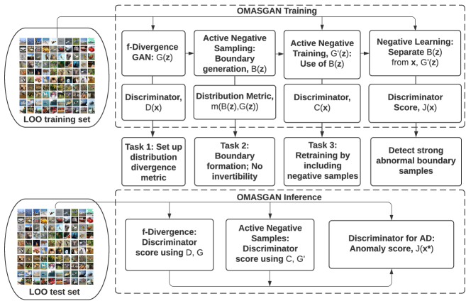
2 Our Proposed OMASGAN Algorithm
Overview. We propose OMASGAN to solve the problem of models setting high likelihood and low reconstruction loss to OoD samples which leads to Type II errors (misses of anomalies), decreasing AD performance 28 . Figure 1 shows the flowchart of OMASGAN: (a) Train a f-divergence-based GAN to obtain the generator, , where z is a latent variable. We denote the latent space by . The GAN samples, , and the data, x, lie in the data space, , where . (b) Train a boundary data generator, , to obtain boundary samples to be used as negative points, for active negative sampling. We compute the statistical divergence between and , and we find the boundary of using any f-divergence in its variational representation. The boundary samples lie in .
OMASGAN generates samples corresponding to a generalized notion of the boundary of the support of the data distribution, which is the set of points such that they are OoD and have a minimum anomaly score measured as the f-divergence. OMASGAN generates OoD samples and we incorporate these OoD Minimum Anomaly Score (OMAS) samples in our algorithm. (c) Perform negative retraining using the OMAS samples and the implicit distributions from (a) and (b), and train the generator using a discriminator, . The samples lie in . OMASGAN performs model retraining and subsequently trains a discriminator for AD using the learned distribution boundary. We train the discriminator for AD using the OMAS samples and active negative training. During inference, for AD, we compute our proposed anomaly score and detect abnormal samples using and .
OMASGAN comprises the optimization tasks: Task 1. Establishing a distribution metric. We train a f-divergence-based GAN model to learn the data, x. Using , , and ,
| (1) | ||||
Using conjugate functions, , 34 ; 44 and for example , the f-divergence optimization objective of OMASGAN Task 1 is given by
| (2) | ||||
Task 2. Formation of the data distribution’s boundary. To perform active negative sampling, we train the distribution boundary model, . The parameters of are . The optimization is
| (3) | ||||
where is the distribution metric from Task 1, i.e. any f-divergence in its variational representation expressed in terms of the conjugate function, , as in (7) in 34 , where is a variational function taking as input a sample and returning a scalar. The special cases of KL and Pearson are and , respectively. The first term in (3) is a strictly decreasing function of a distribution metric. This divergence is between the boundary samples and the data where is the distribution metric of choice, such as Jensen-Shannon of the original GAN, Kullback–Leibler (KL), and Pearson Chi-Squared of the Least Squares GAN 27 to address saturation and mode collapse. The proposed boundary model does not need probability and invertibility obviating the rarity sampling complexity problem by using a decreasing function of a statistical divergence distribution metric, including any f-divergence, to find the data distribution boundary.
Generating the OMAS distribution and OMAS samples: We find minimum-anomaly-score OoD samples and perform learned negative data augmentation eliminating the need for feature extraction and human intervention. This strengthens applicability. We use a f-divergence GAN discriminator to compute the distribution metric, . The first two terms in (3) lead the samples to the boundary of . We compute the boundary with -norm distance and dispersion regularization. We denote the -norm distance between the point and the set x by . To capture all the modes of the data distribution, avoid mode collapse 11 ; 2 , and generate OMAS samples, we use the scattering measure . The distance measure, , and are given by
| (4) | |||
| (5) |
where the batch and inference sizes are denoted by and , respectively. A variation of our point-set distance, , can be obtained by the Chamfer statistical divergence 32 . Good modeling is achieved by finding the boundary of a model of x rather than of x. OMASGAN finds the minimum-anomaly score OoD samples, performs active sampling of negative examples, and generates strong and specifically adversarial anomalies. Strong anomalies lie close to the data distribution boundary while adversarial anomalies are strong anomalies that are close to high-probability data samples.
We use the output of Task 1, , as it has established and set up a distribution metric in . In Task 1, OMASGAN uses a f-divergence-based GAN for data distribution generation. Task 2 performs active negative sampling and trains a boundary generator to form the boundary. We avoid mode collapse and use a relaxed form of the constrained optimization problem of maximizing dispersion subject to being on the f-divergence boundary. In (3), and are hyperparameters. In Task 3, OMASGAN performs active negative training with the minimum-anomaly-score OoD boundary samples, and trains a discriminator, , to classify normal data and abnormal samples, as shown in Figure 2.
Task 3. Active negative training. Separation of generated and real normal from generated abnormal data for AD: To address the learning-OoD-samples problem of 28 ; 21 , we perform retraining for AD by including the negative samples generated by our negative samples augmentation methodology in Task 2. OMASGAN introduces self-supervision by using the learned data distribution boundary from Task 2. We negatively retrain by including the abnormal OoD . To train , we use
| (6) | ||||
where lie in and where is a discriminator which computes distribution metrics and f-divergences, as in 51 ; 6 . To calculate statistical divergences between distributions, and in this case between and , we use a discriminator and a weighted sum of f-divergences and probability metrics 51 ; 6 . The proposed nested optimization in (6) comprises four terms and outputs the learned mappings , where the data space is denoted by , and , where is the latent space. The trainable models are the implicit generator and the discriminator , while and are non-trainable. The first and fourth terms of the minmax optimization force the generated samples to the data, as in Rumi-GAN 6 . The third term forces the generated samples away from our generated strong anomalies, which are near the support boundary of the data distribution and close to high-probability data samples. The discriminator, , is trained to separate from . learns the data, x, keeping away from and avoiding the generated abnormal .
OMASGAN computes the optimal points for negative sampling in Task 2. It performs active negative training using the boundary. The samples from are the closest points to the normal class data and optimal retraining is performed. This leads to improvements with respect to 51 ; 35 ; 41 . We bias the GAN generator to avoid negative samples, improving the AD performance. In contrast to 13 ; 8 , we do not use feature engineering; this strengthens scalability. OMASGAN performs automatic negative samples augmentation and retraining for AD by eliminating the need for feature extraction, human intervention, and ad hoc methods. This strengthens applicability and generalization. Our learned negative data augmentation and retraining methodology incorporates prior knowledge through OoD boundary samples. It is complementary to traditional in-distribution data augmentation methods.
Detection of strong abnormal boundary samples. To address the learning-OoD-samples problem and to perform active negative training for OoD detection, we train the discriminative model ,
| (7) | ||||
Inputs to final negative training: The inputs to are x and samples from . The inputs to and are samples from . Output: which learns to separate from normality, x and .
Our inference mechanism. We use the Anomaly Discriminator, , and the f-divergence distribution metric for AD. The f-divergence is used for training and we also use it during inference. The GAN discriminator computes f-divergences; for the distributions and , we write this metric as fD(, ). We compute fD(, ) for a test sample where is the learned data distribution after retraining and is a Dirac function centered at . For any , the Anomaly Score (AS) is given by
| (8) | ||||
The classification decision is: is from the normal class if , where is a predefined threshold, and is abnormal otherwise. By including negative samples, learns to discriminate between the data distribution and its complement. We leverage to detect OoD samples 51 . OMASGAN generates minimum-anomaly-score OoD samples and subsequently trains using the learned/generated boundary. We use negative training by generating OoD data on the data distribution’s boundary since our model samples from the boundary of the data distribution.
Properties of OMASGAN. Task 1: Let lie in , in and in . Task 1 attains a global optimum, , and convergence to a local optimum is guaranteed 34 . Task 2 Global Properties: Let be the loss in (3) which is a continuous function of . Let the set over which vary be compact. Then, (3) attains a global minimum at . A continuous function defined on a compact set attains a global minimum and maximum: Weierstrass Extreme Value Theorem. (3) attains a global minimum; it is continuous as a function of the parameters of and , (3)-(5) are continuous, and the set over which vary is compact, i.e. sufficient condition.
Local properties. Proposition: Let be the locality where our Task 2 converges. Then, wherever we terminate, that point leads to be a distribution on the boundary. We find such that the distribution on is evenly distributed on the boundary surface manifold, defined as the set of parameters . Necessary condition: which defines the tangent plane to the manifold. We find a boundary distribution; this distribution is evenly distributed on the support boundary of the data distribution. Solving is a hard constrained optimization problem. We introduce a regularized loss instead of a much harder constrained optimization. We regularize and solve . By choosing the hyperparameters and appropriately, we find points in . Gradient Descent finds a local minimum of this combined loss. Using Gradient Descent 53 , the solution to the first two terms in (3) and (4), with the third term in (5), lies on the OMAS manifold. If the loss is locally convex, (3) attains a local minimum. When Task 2 converges at , dispersion is maximized. Mode collapse is eliminated because of the scattering measure in (3) and its combination with the other loss terms.
Global and local properties of Task 3. Let be the boundary distribution from (3). Task 3 in (6) attains a global optimum, . Using both positive and negative samples, learns the distribution of the samples from the positive class 6 ; 51 . The global optimum at subject to both and subsumes that at as a special case and using alternating Stochastic Gradient Descent, convergence to a local optimum is guaranteed 6 .
Let be the loss in (7). The set over which vary is compact and (7) is continuous as a function of the model parameters. It attains a global minimum at such that is lowest, using the Extreme Value Theorem (sufficient condition). Local properties: Let be the point where (7) converges. Wherever OMASGAN terminates, that leads to separate the data distribution from its complement. The model samples points from the distribution boundary as is an implicit distribution on the boundary producing OMAS points for negative training.
3 Related Work
OMASGAN addresses the rarity of abnormal data and provides negative data augmentation by creating strong OoD data on the distribution boundary, unlike 46 ; 42 . Our methodology performs sampling of negative points, creates optimal points for negative training closest to the data, and does not need to know any data features, in contrast to 41 which needs to have a process that programmatically creates the OoD examples using image transformations. OMASGAN learns to generate OoD samples. We perform retraining using active negative sampling setting the boundary points as strong anomalies. This is our contribution and this differs from creating OoD samples by using (i) low-epoch reconstructions 51 ; 35 , (ii) rotated features 41 , and (iii) a CVAE 9 . Old is Gold (OGNet) uses weak anomalies far from the boundary, low-quality reconstructions, and pseudo-anomalies generated in an ad hoc manner without any guarantee of coverage of the OoD part of the data space. OGNet uses a pseudo-anomaly module to create OoD points. It uses a restrictive definition of anomaly as single-epoch blurry reconstructions. It modifies the role of the discriminator (f-divergence distribution metrics) by using an Autoencoder (AE) to distinguish good from bad quality reconstructions. For good and poor quality samples, a generator and an old state of the same AE generator are used. Anomalies that are far away from the boundary are also created by 9 .
Minimum Likelihood GAN (MinLGAN) and FenceGAN generate boundary samples to subsequently use the discriminator score for AD 49 ; 30 . In contrast to the Boundary of Distribution Support Generator (BDSG) 11 , OMASGAN uses any f-divergence distribution metric, no invertibility, and a discriminator for AD. OMASGAN maximizes dispersion subject to being on the f-divergence boundary without mode collapse using a relaxed form of a constrained optimization problem. Our self-supervised learning methodology involves model retraining by including the learned distribution boundary. As opposed to others, OMASGAN makes no assumptions about the data distribution and is not ad hoc. AD is an automatic outcome of our generalized OMASGAN methodology which can improve upon many of the existing techniques to more accurately and more robustly learn .
The rarity of anomalies is not addressed by 37 ; 6 which highlight the benefit of supervision. Rarity is addressed by GEOM 13 , GOAD 8 , and Deep Robust One Class Classification (DROCC) 16 . GEOM trains a multi-class model to discriminate between geometric image transformations, horizontal flipping, translations, and rotations. It learns feature detectors that identify anomalies based on the model’s softmax activation statistics. The classification-based model GOAD generalizes transformation-based methods using affine and geometric transformations. DeepSVDD 36 minimizes the volume of a hypersphere to enclose the data in the latent space using a deep kernel-based AD loss. Mappings of anomalies lie outside, while mappings of normality lie within the hypersphere. However, DeepSVDD suffers from representation collapse. Representations richer than a hypersphere are needed. DROCC is robust to representation collapse and assumes that the data lie on a locally linear well-sampled low-dimensional manifold, but it does not find the distribution boundary.
Table 1 presents a summary of the main characteristics of OMASGAN and the benchmarks. We focus on the key properties of OMASGAN and on the different approaches of GAN, AE, and classification. We highlight the differences in the losses (active negative training, boundary loss) and in the inference mechanism (discriminator anomaly score). In contrast to others, OMASGAN performs active negative sampling and introduces self-generated labels and supervision. It is a GAN and this is desirable since (a) a distribution metric is established in , (b) GANs and distribution metrics have been shown to outperform AEs and distance metrics, and (c) contextual anomalies that have shared features with the data cannot be detected using a reconstruction anomaly score, i.e. near low probability samples.
| OMAS | MinL | Fence | EGB | Ano | Tail | BDSG | OG | Deep | VAE | GAN | GEOM | GO | DR | |
| GAN | GAN | GAN | AD | GAN | GAN | Net | SAD | omaly | AD | OCC | ||||
| 49 | 30 | 52 | 39 | 12 | 11 | 51 | 37 | 52 | 4 | 13 | 8 | 16 | ||
| GAN-based | ||||||||||||||
| AE-based | ||||||||||||||
| Classification | ||||||||||||||
| ANST | ||||||||||||||
| NT | ||||||||||||||
| Boundary | ||||||||||||||
| fD | ||||||||||||||
| Discr. AS | ||||||||||||||
| Reconstruction | ||||||||||||||
| Likelihood |
ANST = Active Negative Sampling and Training; NT = Negative Training; fD = f-Divergence; Discr. AS = Discriminator Anomaly Score
4 Evaluation of OMASGAN
We evaluate OMASGAN using the AUROC. The LOO methodology is used; we set classes of a dataset with classes as the normal class and the leave-out class as the abnormal class. LOO evaluation is more challenging than One Class Classification (OCC) evaluation used by MinLGAN, OGNet, and 43 ; 31 ; 20 which is setting a single class of a dataset as normal and all the remaining classes of the dataset as the abnormal class. The LOO evaluation methodology is more realistic and closer to real-world scenarios than OCC evaluation 3 , as OCC oversimplifies the AD problem.
Models. We train dense fully-connected network architectures for synthetic data and Convolutional Neural Networks (CNN) with batch normalization for image data. We use the recently developed f-divergence-based KL-Wasserstein GAN model (KLWGAN) 44 and the f-GAN model 34 .
Benchmarks. We evaluate OMASGAN using LOO on MNIST and compare it to the GAN models EGBAD 52 and AnoGAN 39 , to the likelihood-based AD models BDSG and TailGAN 11 ; 12 , and to the AE models GANomaly and VAE. We also evaluate OMASGAN using LOO on CIFAR-10 and compare it to EGBAD, AnoGAN, BDSG, GANomaly, VAE, and FenceGAN 30 . We also compare OMASGAN to GOAD, GEOM, DROCC, and DeepSVDD using OCC on CIFAR-10.
Implementation and training. In the LOO setting, the MNIST and CIFAR-10 datasets are transformed into ten AD tasks, where one class is used as the abnormal class and the remaining classes are treated as samples from the normal class. In OCC, CIFAR-10 is transformed into ten AD tasks, where one class is the normal class and the remaining classes are abnormal. The training and validation sets for OMASGAN contain only samples from the normal class. This scenario resembles typical real-world situations where anomalies are rare and not available during training 31 ; 45 . We traverse a set of hyperparameters empirically chosen for Task 2 in (3) and Task 3 in (6) and (7) using a validation set that contains only normal class samples. The validation set of the normal class samples is also used to early stop the training. We select the hyperparameters that lead to the lowest values for the individual loss terms. We observe that from task to task, as well as from dataset to dataset, each term of our losses is not sensitive to the hyperparameters. The hyperparameter values that achieve good performance do not vary across AD tasks, and they prove to be robust across datasets too.
![[Uncaptioned image]](/html/2110.15273/assets/x3.png)
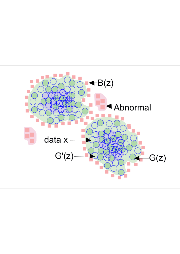
where the blue points are x and the green .
Evaluation of OMASGAN on synthetic data. We train the proposed f-divergence-based OMASGAN on synthetic data in Figure 3. The evaluation on synthetic data shows that OMASGAN generates abnormal OoD data on the boundary of the distribution support. Figure 3 shows the OMAS samples, i.e. the green points. The blue points are samples from the data distribution. We show that OMASGAN eliminates mode collapse and works for multimodal data distributions with a support with disconnected components 31 ; 37 ; 30 . Our scattering term in (3) and (5) preserves distance proportionality in and , eliminating mode collapse. OMASGAN achieves dispersion using in Section 2, not requiring the calculation of the center of mass of the data distribution. OMASGAN obviates the sampling complexity problem and the parallel estimation of the mass and the boundary. We continue the evaluation of OMASGAN on synthetic data, and we evaluate OMASGAN using histograms of anomaly scores. With retraining, we increase the AUROC metric and the Area Under the Precision-Recall Curve (AUPRC) from to and the F1 score, Precision, Recall, and Accuracy from to on a grid of equidistant points.
Evaluation of OMASGAN on MNIST. Setup: We evaluate the proposed f-divergence-based OMASGAN model using the LOO methodology. We train OMASGAN using the KLWGAN until convergence, approximately epochs. We use CNN architectures for generating the distributions , , and . We use , , , , and in Section 2. We train OMASGAN and successfully generate , , and . We evaluate OMASGAN and its discriminator using histograms of the anomaly scores for normal and abnormal samples.
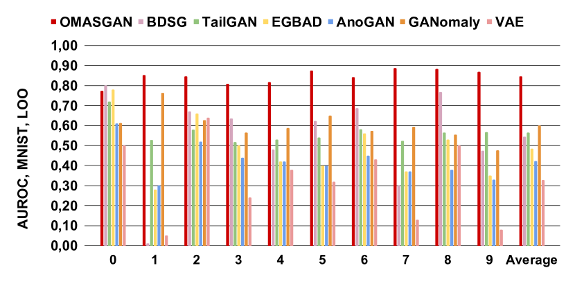
LOO Evaluation in AUROC: Figure 4 shows that on average and for all the MNIST digits, OMASGAN outperforms the GAN benchmarks EGBAD, AnoGAN, BDSG, and TailGAN. Also, Figure 4 shows that OMASGAN outperforms the AE-based models GANomaly and VAE. We evaluate OMASGAN and compare it with GANomaly using the same inference conditions as those in OMASGAN, i.e. training set statistics rather than test set statistics for the batch normalization layers. Figure 4 shows that OMASGAN achieves on average an AUROC of on MNIST and outperforms the benchmarks by at least points in AUROC, by a percentage of . The proposed OMASGAN model is robust and achieves the lowest standard deviation (SD) averaged over all the MNIST digits, i.e. , compared to EGBAD, AnoGAN, BDSG, TailGAN, GANomaly, and VAE. These AD benchmarks have SDs averaged over all the digits , , , , , and , respectively.
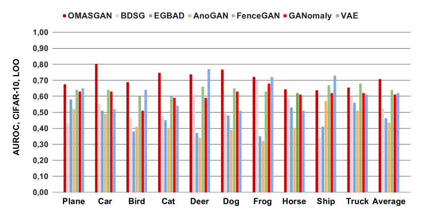
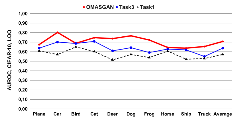
Evaluation of OMASGAN on CIFAR-10. Setup: In (6) and (7) in Section 2, we use , , and , as in 6 ; 51 . LOO Evaluation in AUROC: Figure 5 shows that the performance of OMASGAN using LOO is better than that of the GAN models AnoGAN, EGBAD, FenceGAN, and BDSG on average and for all tasks. In Figure 5, on average and for almost all classes, the proposed OMASGAN outperforms the AE benchmarks GANomaly, VAE, ADAE, and AED. According to Figure 5, OMASGAN outperforms the benchmarks in AUROC averaged over all classes. It is robust achieving the lowest SD, , compared to the AD benchmarks. It outperforms the benchmarks on average over all tasks by at least AUROC points, by a percentage increase of at least . OMASGAN achieves on average an AUROC of on CIFAR-10 using LOO evaluation. On the CIFAR-10 dataset, it achieves an improvement of approximately compared to benchmarks.
UROC on MNIST data using LOO evaluation.
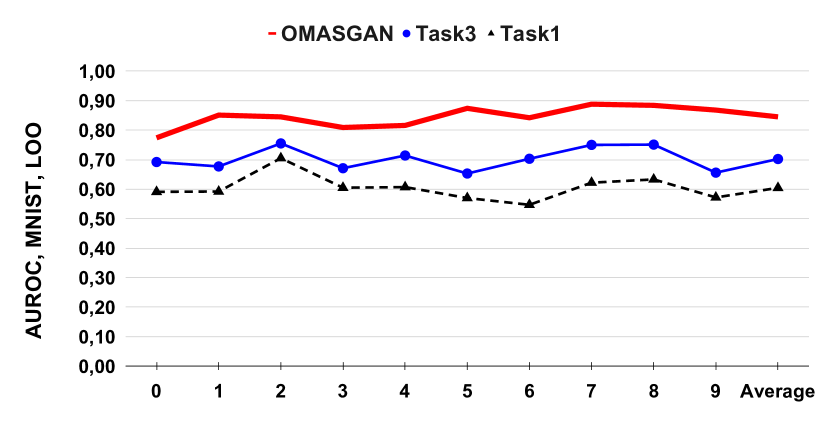
Ablation study/analysis of OMASGAN. Benefit of model retraining by including negative boundary samples: OMASGAN trained on MNIST: Figure 6 shows that, on average and for all the MNIST digits, OMASGAN improves the performance of the KLWGAN model implemented in Task 1 for OoD detection. Comparing the training objective in Task 1 to the loss in Task 3 and to the final loss, OMASGAN improves the performance of the base model. The base model KLWGAN achieves an AUROC of averaged over all the MNIST digits, increasing to using Task 3, and then to using our final OMASGAN model. This is the contribution of our proposed Tasks 2 and 3.
Effect of base model and chosen f-divergence. In Figure 7, we compare OMASGAN using the KLWGAN to the OMASGAN using the f-GAN on MNIST in AUROC 44 ; 34 . According to the ablation study, OMASGAN improves the performance of f-GAN by on average over all digits. The base model f-GAN achieves on average an AUROC of , which increases to because of OMASGAN Task 3. Figure 7 shows the benefit of the OMASGAN properties of active negative sampling and training, learned negative data augmentation, boundary loss training, and discriminator anomaly score inference, presented in Table 1. We also observe robustness across the AD tasks.
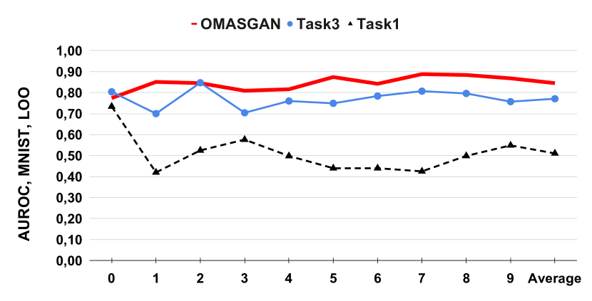
Improvement of OMASGAN compared to KLWGAN for AD on CIFAR-10. Figure 8 presents an ablation study on the losses of OMASGAN on CIFAR-10 in AUROC using the LOO evaluation methodology. We examine the impact of all our objective cost functions on the anomaly and OoD detection performance in Figure 8. Our chosen base model, KLWGAN, yields an AUROC of averaged over all the LOO classes and this increases to using OMASGAN Task 3 and to using OMASGAN. In reference to Table 1, Figure 8 shows that the improvement of points in AUROC is the contribution of our retraining and negative data augmentation methodology. This is the benefit of the proposed active negative and boundary loss training in Section 2. The average SD over all the LOO classes is , , and for Task1, Task3, and OMASGAN, respectively.
Effect of selected inference mechanism. Following our discussion in Section 2, the anomaly score for a test sample is fD(, ) and fD(, ) if the OMASGAN model is stopped at Task 3 and Task 1, respectively, in the ablation study in Figures 6-8. Comparing OMASGAN to Tasks 1 and 3, the performance gradually improves and the use of , as presented in Section 2, is beneficial.
Sensitivity to initialization. Figure 9 shows the sensitivity of OMASGAN on CIFAR-10 to changes to the random seeds , , and . It shows the mean AUROC over all seeds per LOO class, the AUROC for seed , and the mean AUROC SD. The performance of OMASGAN yields a difference between seeds. The mean SD over all classes and seeds is and this is lower than that of 37 which is . The mean SD per seed over all classes is for seed , and for seeds and .
AUROC on CIFAR-10 data using OCC evaluation.
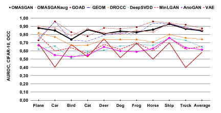
Evaluation of OMASGAN on CIFAR-10 using OCC. In Figure 10, we evaluate OMASGAN and compare it to GAN and AE models, and to GOAD and GEOM. Our model achieves an average AUROC of . It outperforms the GAN models AnoGAN and MinLGAN, and the AE models VAE and DeepSVDD. OMASGAN also outperforms the discriminator-based model DROCC. OMASGAN achieves robustness across the AD tasks. OMASGANaug uses data augmentation comprising geometric image transformations, i.e. horizontal flipping and color augmentation, during training and slightly improves the AD performance of OMASGAN. The performance of OMASGAN and OMASGANaug is comparable to that of the classification model GEOM. GOAD uses data augmentation comprising geometric image transformations, e.g. flips and rotations, as well as affine transformations, and slightly outperforms OMASGANaug on average by approximately . The classification-based models GEOM and GOAD use features to discriminate between transformations. On the contrary, OMASGAN does not use feature engineering, human intervention, and manual processes. This is desirable and strengthens scalability and applicability.
5 Discussion and Conclusion
We have proposed OMASGAN, a retraining methodology for AD with active negative sampling and training and self-supervised learning. OMASGAN performs negative retraining by including the generated boundary which has the effect of “pushing” the distribution away from the OoD samples to improve the learning of the data distribution. AD is a direct outcome of retraining which can be used in conjunction with existing models. The proposed retraining methodology does not make any assumptions about the underlying data distribution, is not ad hoc, and is data- and architecture-agnostic. OMASGAN performs learned data augmentation and AD using negative sampling. Without requiring invertibility or likelihood, we generate OMAS samples and strong anomalies leveraging any f-divergence in its variational representation. OMASGAN does not use feature engineering and works for data distributions with a support with disconnected components without mode collapse. We address the rarity of anomalies using data only from the normal class. We use the discriminator to compute distribution metrics as they permit the modelling of rarity, taking into account the weak property of f-divergences and the evolution of generative models from AEs to GANs. The evaluation outcomes on MNIST and CIFAR-10, as well as on synthetic data, using the LOO methodology show that OMASGAN achieves state-of-the-art performance and outperforms the GAN- and AE-based benchmarks, as illustrated in Figures 4 and 5. The ablation study in Figures 6-8 shows that OMASGAN improves the base model for AD using LOO evaluation on MNIST and CIFAR-10. Using the AUROC, OMASGAN yields on average (i) an improvement of at least points on MNIST over the benchmarks, achieving values of , and (ii) an improvement of at least points on CIFAR-10, achieving values of using the LOO methodology. LOO evaluation is more realistic than OCC; in real-world scenarios, we have a large number of items that are not rare and we are interested in detecting the objects that are significantly different from these items. Figure 10 illustrates that OMASGAN outperforms the GAN and AE benchmarks MinLGAN, AnoGAN, VAE, DeepSVDD, and the discriminator-based DROCC on CIFAR-10 using OCC evaluation, and achieves an average AUROC of . OMASGAN also achieves robustness across the different AD tasks.
References
-
(1)
Abbasnejad, M., Shi, J., van den Hengel, A., and Liu, L., “A Generative Adversarial Density Estimator,” in Proceedings IEEE/CVF International Conference on Computer Vision and Pattern Recognition (CVPR), pp. 10774-10783, Long Beach, CA, USA, June 2019. DOI: 10.1109/CVPR.2019.01104.
Online: https://ieeexplore.ieee.org/document/8953918 -
(2)
Abbasnejad, M., Shi, J., van den Hengel, A., and Liu, L., “GADE: A Generative Adversarial Approach to Density Estimation and its Applications,” International Journal of Computer Vision, pp. 2731-2743, vol. 128, no. 10, August 2020. DOI: 10.1007/s11263-020-01360-9.
Online: https://link.springer.com/article/10.1007/s11263-020-01360-9 -
(3)
Ahmed, F. and Courville, A., “Detecting Semantic Anomalies,” in Proceedings of the AAAI Conference on Artificial Intelligence, vol. 34 (04), pp. 3154-3162, 2020. DOI: 10.1609/aaai.v34i04.5712.
Online: https://openreview.net/pdf?id=0JQHVDNuElN -
(4)
Akcay, S., Atapour-Abarghouei, A., and Breckon, T., “GANomaly:
Semi-supervised Anomaly Detection via Adversarial Training”, in Proceedings 14th Asian Conference on Computer Vision (ACCV), pp. 622-637, vol. 11363, Lecture Notes in Computer Science, Springer, Cham, 2019. DOI: 10.1007/978-3-030-20893-639.
Online: https://link.springer.com/chapter/10.1007/978-3-030-20893-639 -
(5)
Akcay, S., Atapour-Abarghouei, A., and Breckon, T., “Skip-GANomaly: Skip Connected and Adversarially Trained Encoder-Decoder Anomaly Detection”, in Proceedings IEEE International Joint Conference on Neural Networks (IJCNN), pp. 1-8, Budapest, Hungary, July 2019. DOI: 10.1109/IJCNN.2019.8851808.
Online: https://ieeexplore.ieee.org/document/8851808 -
(6)
Asokan, S. and Seelamantula, C., “Teaching a GAN What Not to Learn,” in Proceedings 34th Conference on Neural Information Processing Systems (NeurIPS 2020), Larochelle, H., Ranzato, M., Hadsell, R., Balcan, M., and Lin, H. (eds), Vancouver, Canada, December 2020.
Online: https://papers.nips.cc/paper/2020/file/29405e2a4c22866a205f557559c7fa4b-Paper.pdf -
(7)
Author, “OoD Minimum Anomaly Score GAN - Code for the Paper OMASGAN: Out-of-Distribution Minimum Anomaly Score GAN for Sample Generation on the Boundary,” GitHub Repository, 2021.
Online: https://github.com/Anonymous-Author-2021/OMASGAN
Online: https://anonymous.4open.science/r/OMASGAN-5702/README.md -
(8)
Bergman, L. and Hoshen, Y., “Classification-Based Anomaly Detection for General Data,” in Proceedings International Conference on Learning Representations (ICLR), 2020.
Online: https://openreview.net/pdf/0cc1c7474fb7a5d646d371f84aef56b3e920caa7.pdf -
(9)
Bhatia, S., Jain, A., and Hooi, B., “ExGAN: Adversarial Generation of Extreme Samples,” in Proceedings 35th Association for the Advancement of Artificial Intelligence (AAAI) Conference on Artificial Intelligence, AAAI-2050, Virtual Conference, February 2021.
Online: https://www.aaai.org/AAAI21Papers/AAAI-2050.BhatiaS.pdf - (10) Bian, J., Hui, X., Sun, S., Zhao, X., and Tan, M., “A Novel and Efficient CVAE-GAN-Based Approach With Informative Manifold for Semi-Supervised Anomaly Detection,” in IEEE Access, vol. 7, pp. 88903-88916, 2019. Online: https://ieeexplore.ieee.org/document/8727990
- (11) Brock, A., Donahue, J., and Simonyan, K., “Large Scale GAN Training for High Fidelity Natural Image Synthesis,” in Proceedings Seventh International Conference on Learning Representations (ICLR), New Orleans, Louisiana, USA, May 2019. Online: https://openreview.net/pdf?id=B1xsqj09Fm
-
(12)
Dionelis, N., Yaghoobi, M., and Tsaftaris, S., “Boundary of Distribution Support Generator (BDSG): Sample Generation on the Boundary,” in Proceedings IEEE International Conference on Image Processing (ICIP), pp. 803-807, October 2020. DOI: 10.1109/ICIP40778.2020.9191341.
Online: https://ieeexplore.ieee.org/document/9191341 -
(13)
Dionelis, N., Yaghoobi, M., and Tsaftaris, S., “Tail of Distribution GAN (TailGAN): Generative-Adversarial-Network-Based Boundary Formation,” in Proceedings Sensor Signal Processing for Defence (SSPD) IEEE Conference, pp. 41-45, November 2020. DOI: 10.1109/SSPD47486.2020.9272100.
Online: https://ieeexplore.ieee.org/abstract/document/9272100 -
(14)
Golan, I. and El-Yaniv, R., “Deep Anomaly Detection Using Geometric Transformations,” in Proceedings Advances in Neural Information Processing Systems (NeurIPS), pages 9758-9769, 2018.
Online: https://papers.nips.cc/paper/2018/file/5e62d03aec0d17facfc5355dd90d441c-Paper.pdf -
(15)
Gong, D., Liu, L., Le, V., Saha, B., Mansour, M., Venkatesh, S., and van den Hengel, A., “Memorizing Normality to Detect Anomaly: Memory-Augmented Deep Autoencoder for Unsupervised Anomaly Detection,” in Proceedings IEEE/CVF International Conference on Computer Vision (ICCV), Seoul, Korea (South), pp. 1705-1714, November 2019. DOI: 10.1109/ICCV.2019.00179.
Online: https://ieeexplore.ieee.org/abstract/document/9010977 -
(16)
Goodfellow, I., Pouget-Abadie, J., Mirza, M., Xu, B., Warde-Farley, D., Ozair, S., Courville, A., and Bengio, Y., “Generative Adversarial Nets,” in Proceedings Advances in Neural Information Processing Systems 27 (NIPS 2014), pp. 2672–2680, Montréal, Canada, December 2014.
Online: https://papers.nips.cc/paper/2014/file/5ca3e9b122f61f8f06494c97b1afccf3-Paper.pdf -
(17)
Goyal, S., Raghunathan, A., Jain, M., Simhadri, H., and Jain, P., “DROCC: Deep Robust One-Class Classification,” in Proceedings International Conference on Machine Learning (ICML), 2020.
Online: https://arxiv.org/pdf/2002.12718.pdf - (18) Hendrycks, D., Mazeika, M., and Dietterich, T., “Deep Anomaly Detection with Outlier Exposure,” in Proceedings Seventh International Conference on Learning Representations (ICLR 2019), New Orleans, Louisiana, USA, May 2019. Online: https://openreview.net/pdf?id=HyxCxhRcY7
- (19) Hjelm, R., Jacob, A., Che, T., Trischler, A., Cho, K., and Bengio, Y., “Boundary-Seeking Generative Adversarial Networks,” in Proceedings Sixth International Conference on Learning Representations (ICLR), Vancouver, Canada, May 2018. Online: https://openreview.net/pdf?id=rkTS8lZAb
-
(20)
Jalal, A., Ilyas, A., Dimakis, A., and Daskalakis, C., “The Robust Defense: Adversarial Training Using Generative Models,” arXiv preprint, arXiv:1712.09196 [cs.CV], July 2019.
Online: https://arxiv.org/pdf/1712.09196.pdf - (21) Kim, Y., Kwon, Y., Chang, H., and Paik, M., “Lipschitz Continuous Autoencoders in Application to Anomaly Detection,” in Proceedings of the 23rd International Conference on Artificial Intelligence and Statistics (AISTATS), pp. 2507-2517, vol. 108, Chiappa, S. and Calandra, R. (eds), Palermo, Italy, August 2020. Online: http://proceedings.mlr.press/v108/kim20c/kim20c.pdf
-
(22)
Kirichenko, P., Izmailov, P., and Wilson, A., “Why Normalizing Flows Fail to Detect Out-of-Distribution Data,” in Proceedings 34th Conference on Neural Information Processing Systems (NeurIPS 2020), Vancouver, Canada, December 2020.
Online: https://proceedings.neurips.cc/paper/2020/file/ecb9fe2fbb99c31f567e9823e884dbec-Paper.pdf - (23) Krizhevsky, A., “Learning Multiple Layers of Features from Tiny Images,” Technical Report, TR-2009, University of Toronto, Toronto, April 2009. Online: https://www.cs.toronto.edu/ kriz/cifar.html
- (24) LeCun, Y. and Cortes, C., “MNIST Handwritten Digit Database,” 2010. http://yann.lecun.com/exdb/mnist/
- (25) Lee, K., Lee, H., Lee, K., and Shin, J., “Training Confidence-Calibrated Classifiers for Detecting Out-of-Distribution Samples,” in Proceedings 6th International Conference on Learning Representations (ICLR), Vancouver, Canada, May 2018. Online: https://openreview.net/pdf?id=ryiAv2xAZ
- (26) Liznerski, P., Ruff, L., Vandermeulen, R., Franks, B., Kloft, M., and Muller, K., "Explainable Deep One-Class Classification," in Proceedings International Conference on Learning Representations (ICLR), 2021. Online: https://openreview.net/pdf?id=A5VV3UyIQz
-
(27)
Maaløe, L., Fraccaro, M., Liévin, V., and Winther, O., “BIVA: A Very Deep Hierarchy of Latent Variables for Generative Modeling,” in Proceedings 33rd Conference on Neural Information Processing Systems (NeurIPS 2019), Vancouver, Canada, December 2019.
Online: https://papers.nips.cc/paper/2019/file/9bdb8b1faffa4b3d41779bb495d79fb9-Paper.pdf - (28) Mao, X., Li, Q., Xie, H., Lau, R., Wang, Z., and Smolley, S., “Least Squares Generative Adversarial Networks,” in Proceedings IEEE International Conference on Computer Vision (ICCV), pp. 2813-2821, Venice, Italy, October 2017. DOI: 10.1109/ICCV.2017.304. Online: https://ieeexplore.ieee.org/document/8237566
- (29) Nalisnick, E., Matsukawa, A., Teh, Y., Gorur, D., and Lakshminarayanan, B., “Do Deep Generative Models Know What They Don’t Know?,” in Proceedings Seventh International Conference on Learning Representations (ICLR), New Orleans, USA, May 2019. Online: https://openreview.net/pdf?id=H1xwNhCcYm
- (30) Netzer, Y., Wang, T., Coates, A., Bissacco, A., Wu, B., and Ng, A., “Reading Digits in Natural Images with Unsupervised Feature Learning,” NIPS Workshop on Deep Learning and Unsupervised Feature Learning, 9 pages, December 2011. Online: http://ufldl.stanford.edu/housenumbers/
-
(31)
Ngo, P., Winarto, A., Li Kou, C., Park, S., Akram, F., and Lee, H., “Fence GAN: Towards Better Anomaly Detection”, in Proceedings IEEE 31st International Conference on Tools with Artificial Intelligence (ICTAI), pp. 141-148, Portland, Oregon, USA, November 2019. DOI: 10.1109/ICTAI.2019.00028.
Online: https://ieeexplore.ieee.org/document/8995288 -
(32)
Nguyen, D., Lou, Z., Klar, M., and Brox, T., “Anomaly Detection with Multiple-Hypotheses Predictions,” in Proceedings International Conference on Machine Learning (ICML), pp. 4800-4809, vol. 97, Chaudhuri, K. and Salakhutdinov, R. (eds), Long Beach, California, USA, June 2019.
Online: http://proceedings.mlr.press/v97/nguyen19b/nguyen19b.pdf -
(33)
Nguyen, T., Pham, Q., Le, T., Pham, T., Ho, N., and Hua, B., “Point-set Distances for Learning Representations of 3D Point Clouds,” arXiv preprint, arXiv:2102.04014 [cs.CV], Febr. 2021.
Online: https://arxiv.org/pdf/2102.04014.pdf -
(34)
Nielsen, F., and Nock, R., “On the Chi Square and Higher-Order Chi Distances for Approximating f-Divergences,” IEEE Signal Processing Letters, pp. 10-13, vol. 21, no. 1, January 2014. DOI: 10.1109/LSP.2013.2288355.
Online: https://ieeexplore.ieee.org/document/6654274 -
(35)
Nowozin, S., Cseke, B., and Tomioka, R., “f-GAN: Training Generative Neural Samplers using Variational Divergence Minimization,” in Proceedings Thirtieth Conference on Neural Information Processing Systems (NeurIPS), Barcelona, Spain, December 2016.
Online: https://papers.nips.cc/paper/2016/file/cedebb6e872f539bef8c3f919874e9d7-Paper.pdf -
(36)
Pourreza, M., Mohammadi, B., Khaki, M., Bouindour, S., Snoussi, H., and Sabokrou, M., “G2D: Generate to Detect Anomaly,” in Proceedings IEEE/CVF Winter Conference on Applications of Computer Vision (WACV), pp. 2003-2012, Virtual Conference, January 2021.
Online: https://openaccess.thecvf.com/content/WACV2021/papers/PourrezaG2DGeneratetoDetect
AnomalyWACV2021paper.pdf -
(37)
Ruff, L., Vandermeulen, R., Görnitz, N., Binder, A., Müller, E., Müller, K., and Kloft, M., “Deep One-Class Classification,” in Proceedings International Conference on Machine Learning (ICML), pp. 4393-4402, vol. 80, Dy, J. and Krause, A. (eds), Stockholm, Sweden, July 2018.
Online: http://proceedings.mlr.press/v80/ruff18a/ruff18a.pdf -
(38)
Ruff, L., Vandermeulen, R., Görnitz, N., Binder, A., Müller, E., Müller, K., and Kloft, M., “Deep Semi-Supervised Anomaly Detection,” in Proceedings International Conference on Learning Representations (ICLR), Virtual Conference, Formerly Addis Ababa, Ethiopia, May 2020.
Online: https://openreview.net/pdf?id=HkgH0TEYwH -
(39)
Sabokrou, M., Khalooei, M., Fathy, M., and Adeli, E., “Adversarially Learned One-Class Classifier for Novelty Detection,” in Proceedings IEEE/CVF Conference Computer Vision and Pattern Recognition (CVPR), pp. 3379-3388, Salt Lake City, UT, USA, June 2018. DOI: 10.1109/CVPR.2018.00356.
Online: https://ieeexplore.ieee.org/document/8578454 - (40) Schlegl, T., Seeböck, P., Waldstein, S., Schmidt-Erfurth, U., and Langs, G., “Unsupervised Anomaly Detection with GANs to Guide Marker Discovery,” in Proceedings International Conference on Information Processing in Medical Imaging (IPMI), Appalachian State University, Boone, North Carolina, USA, June 2017. Online: https://arxiv.org/pdf/1703.05921.pdf
-
(41)
Sehwag, V., Chiang, M., and Mittali, P., “SSD: A Unified Framework for Self-Supervised Outlier Detection,” in Proceedings International Conference on Learning Representations (ICLR), 2021.
Online: https://openreview.net/pdf?id=v5gjXpmR8J -
(42)
Sinha, A., Ayush, K., Song, J., Uzkent, B., Jin, H., and Ermon, S., “Negative Data Augmentation,” in Proceedings International Conference on Learning Representations (ICLR), May 2021.
Online: https://openreview.net/pdf?id=Ovp8dvB8IBH -
(43)
Sipple, J., “Interpretable, Multidimensional, Multimodal Anomaly Detection with Negative Sampling for Detection of Device Failure,” in Proceedings Thirty-seventh International Conference on Machine Learning (ICML), pp. 9016-9025, vol. 119, Daumé III, H. and Singh, A. (eds), July 2020.
Online: https://icml.cc/media/Slides/icml/2020/virtual(no-parent)-14-21-00UTC-6171-interpretable.pdf
http://proceedings.mlr.press/v119/sipple20a/sipple20a.pdf - (44) Sohn, K., Li, C., Yoon, J., Jin, M., and Pfister, T., "Learning and Evaluating Representations for Deep One-Class Classification," in Proceedings International Conference on Learning Representations (ICLR), 2021. Online: https://openreview.net/pdf?id=HCSgyPUfeDj
-
(45)
Song, J. and Ermon, S., “Bridging the Gap Between f-GANs and Wasserstein GANs,” in Proceedings International Conference on Machine Learning (ICML), pp. 9078-9087, vol. 119, Daumé III, H. and Singh, A. (eds), July 2020.
Online: http://proceedings.mlr.press/v119/song20a/song20a.pdf -
(46)
Sricharan, K. and Srivastava, A., “Building Robust Classifiers Through Generation of Confident Out of Distribution Examples,” Third Workshop on Bayesian Deep Learning (NeurIPS), 2018.
Online: https://arxiv.org/pdf/1812.00239.pdf -
(47)
Sung, Y., Pei, S., Hsieh, S., and Lu, C., “Difference-Seeking GAN - Unseen Sample Generation,” in Proceedings Eighth International Conference on Learning Representations (ICLR), Virtual Conference, Formerly Addis Ababa, Ethiopia, May 2020.
Online: https://openreview.net/pdf?id=rygjmpVFvB -
(48)
Sutherland, D., “Scalable, Flexible, and Active Learning on Distributions,” Carnegie Mellon University, School of Computer Science, PhD Thesis, Pittsburgh, Pennsylvania, USA, September 2016.
Online: http://reports-archive.adm.cs.cmu.edu/anon/2016/CMU-CS-16-128.pdf -
(49)
Vu, H., Ueta, D., Hashimoto, K., Maeno, K., Pranata, S., and Shen, S., “Anomaly Detection with Adversarial Dual Autoencoders,” arXiv preprint, arXiv:1902.06924 [cs.CV], February 2019.
Online: https://arxiv.org/pdf/1902.06924.pdf -
(50)
Wang, C., Zhang, Y., and Liu, C., “Anomaly Detection via Minimum Likelihood Generative Adversarial Networks,” in Proceedings 24th International Conference on Pattern Recognition (ICPR), pp. 1121-1126, Beijing, China, August 2018. DOI: 10.1109/ICPR.2018.8545381.
Online: https://ieeexplore.ieee.org/document/8545381 -
(51)
Xiao, H., Rasul, K., and Vollgraf, R., “Fashion-MNIST: A Novel Image Dataset for Benchmarking Machine Learning Algorithms,” arXiv preprint, arXiv:1708.07747 [cs.LG], September 2017.
Online: https://www.kaggle.com/zalando-research/fashionmnist -
(52)
Zaheer, M., Lee, J., Astrid, M., and Lee, S., “Old is Gold: Redefining the Adversarially Learned One-Class Classifier Training Paradigm,” in Proceedings IEEE/CVF Conference Computer Vision and Pattern Recognition (CVPR 2020), pp. 14171-14181, Seattle, Washington, USA, June 2020. DOI: 10.1109/CVPR42600.2020.01419.
Online: https://ieeexplore.ieee.org/document/9157105 -
(53)
Zenati, H., Foo, C., Lecouat, B., Manek, G., and Chandrasekhar, V., “Efficient GAN-Based Anomaly Detection,” Workshop Track in Sixth International Conference on Learning Representations (ICLR 2018), Vancouver, Canada, May 2018.
Online: https://openreview.net/pdf?id=BkXADmJDM -
(54)
Zhu, Z., Soudry, D., Eldar, Y., and Wakin, M., “The Global Optimization Geometry of Shallow Linear Neural Networks,” Journal of Mathematical Imaging and Vision, pp. 279–292, vol. 62, April 2020. DOI: 10.1007/s10851-019-00889-w.
Online: https://link.springer.com/article/10.1007/s10851-019-00889-w -
(55)
Zhu, Z., Soudry, D., Eldar, Y., and Wakin, M., “Implicit Regularization in Nonconvex Statistical Estimation: Gradient Descent Converges Linearly for Phase Retrieval, Matrix Completion, and Blind Deconvolution,” Foundations of Computational Mathematics (FOCM 2020), pp. 451-632, vol. 20, no. 3, June 2020. DOI: 10.1007/s10208-019-09429-9.
Online: https://link.springer.com/content/pdf/10.1007%2Fs10208-019-09429-9.pdf -
(56)
Zisselman, E. and Tamar, A., “Deep Residual Flow for Out of Distribution Detection,” in Proceedings IEEE/CVF Conference Computer Vision and Pattern Recognition (CVPR), pp. 13991-14000, June 2020.
DOI: 10.1109/CVPR42600.2020.01401.
Online: https://ieeexplore.ieee.org/document/9157674
Appendix and Supplementary Material
The discussions, experiments, and evaluations in this Section are a continuation of the paper “OMASGAN: Out-of-Distribution Minimum Anomaly Score GAN for Sample Generation on the Boundary”.
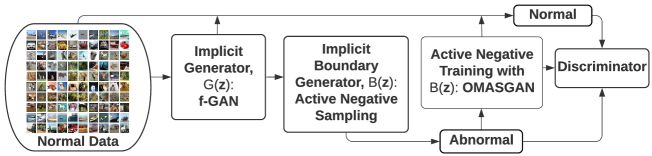
A. OMASGAN and Illustration of our Algorithm
In this section, we present an illustration of the proposed OMASGAN algorithm using the notation and the implicit generative models introduced in Section 2 of the paper.
Figure 11 depicts the main idea of the proposed OMASGAN algorithm. OMASGAN first generates minimum-anomaly-score OoD samples created by our negative sampling augmentation methodology and then performs active negative training for AD. OMASGAN performs model retraining and subsequently trains a discriminative model for AD using the generated samples on the boundary of the support of the data distribution.
B. Implementation of OMASGAN
The proposed OMASGAN model is implemented in PyTorch: https://github.com/Anonymous-Author-2021/OMASGAN
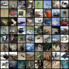
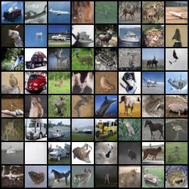
C. Images from OMASGAN Tasks 1 and 3