Four-dimensional hybrid chaos system and its application in creating a secure image transfer environment by cellular automata

Abstract

One of the most important and practical researches which has been considered by researchers is creating secure environments for information exchanges. Due to their structures, chaos systems are efficient tools in the are of data transferring. In this research, using a mathematical structure such as composing and transferring, we improve classical chaotic systems by creating a four-dimensional system. Then we introduce a new encryption algorithm based on the chaos and cellular automata. The security of the proposed environment which is evaluated using different types of security tests shows the efficiency of the proposed algorithm.

^aDepartment of Mathematics, University of Mohaghegh Ardabili, 56199-11367 Ardabil, Iran.

Keywords: Cryptography; Image; Chaotic system; Cellular automata.

1 Introduction

With the rapid development of social networks, a huge amount of various information in the form of text, image, audio and video is exchanged through these networks in any small period of time. Because of their visual features, digital images have been received more attention among other formats, and so it is important to present a new method or improve existing methods in order to transfer images safely. In addition to steganography, cryptography is a method of secure transfer of information in which the goal is to scramble pixels of data properly so that it is not detectable [4]. So far, various cryptographic methods have been proposed based on cellular automata, chaotic mapping, and so on for example see [8, 16, 24]. Chaos systems are nonlinear phenomena with random-like behaviors. These maps are very important in information security transforms with due regard to their special features, which we will discuss in detail in future sections. Given that researchers have shown that algorithms that use existing chaotic maps are likely to be attacked [23], defining appropriate maps is a priority for cryptographic methods. The dimension of a chaos maps are determined based on the number of input and output variables. In general, it can be said that high-dimensional chaotic maps, although having high computational cost, perform better than one-dimensional maps due to their complex dynamic structure.

Cellular automata is one of the image encryption tools that has been used in this article due to its fast, easy and high speed process. In [2], Ray et al use chaos and 3D automation to encode digital images. First, the replacement operation is performed by a chaotic system, and then the diffusion operation is performed using a three-dimensional cellular automata. This method has shown good resistance to most known cryptographic attacks. Wang’s method is an image encryption system based on chaos theory and cellular automation. This method uses a logistic map and reversible cellular automata. Pixel values divided in four-bit units, then in the permutation step of logistic map and the distribution step, cellular automation is also used. This method of cryptography, which is one of the symmetric methods, has good security and shows good resistance against differential attacks [17].

2 4D Hybrid Chaos Systems

In the first step of this section, we introduce a novel type of four-dimensional chaotic system by improving its overall structure, and then in the second subsection, we evaluate the proposed chaos behavior using the various tests such as lyapunov exponent and cobweb diagram.

2.1 Structure of the Proposed Hybrid System

In this subsection, more details about the proposed new hybrid chaos systems based on Tent, Sin and Logistic maps are given. The general structure of the proposed chaos system has been given in Fig. 1. The combination parts in the proposed system based on Tent, Sin and Logistic maps are shown in Fig. 2. The mathematics formulae for each of the parts can be written as follows.

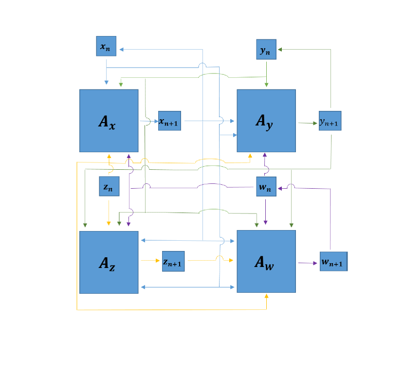
Figure 1: The structure of the proposed chaotic system.

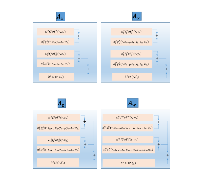
Figure 2: The structure of the combination parts in the proposed system.

-First combination box:

$$x_{i+1}:=\left\{\begin{array}[]{ll}\alpha^{x}_{1}f^{x}_{1}\circ F^{x}_{1}(r,x_{i})+g^{x}_{1}(r,x_{i},y_{i},z_{i},w_{i})\\ ~{}~{}~{}~{}~{}~{}~{}~{}~{}~{}~{}~{}+h_{1}^{x}(\frac{(\beta^{x}_{1}-r)z_{i}}{2})~{}mod~{}1,~{}~{}when~{}w_{i}<0.5,\\ \\ \alpha^{x}_{2}f^{x}_{2}\circ F^{x}_{2}(r,x_{i})+g^{x}_{2}(r,x_{i},y_{i},z_{i},w_{i})\\ ~{}~{}~{}~{}~{}~{}~{}~{}~{}~{}~{}~{}+h_{2}^{x}(\frac{(\beta^{x}_{2}-r)(1-z_{i})}{2})~{}mod~{}1,~{}~{}when~{}w_{i}\geq 0.5.\\ \end{array}\right.$$ (2.6)

-Second combination box:

$$y_{i+1}:=\left\{\begin{array}[]{ll}\alpha^{y}_{1}f^{y}_{1}\circ F^{y}_{1}(r,y_{i})+g^{y}_{1}(r,x_{i+1},x_{i},y_{i},z_{i},w_{i})\\ ~{}~{}~{}~{}~{}~{}~{}~{}~{}~{}~{}~{}+h_{1}^{y}(\frac{(\beta^{y}_{1}-r)\zeta_{1}}{2})~{}mod~{}1,~{}~{}when~{}\zeta_{1}<0.5,\\ \\ \alpha^{y}_{2}f^{y}_{2}\circ F^{y}_{2}(r,y_{i})+g^{y}_{2}(r,x_{i+1},x_{i},y_{i},z_{i},w_{i})\\ ~{}~{}~{}~{}~{}~{}~{}~{}~{}~{}~{}~{}+h_{2}^{y}(\frac{(\beta^{y}_{2}-r)(1-\zeta_{1})}{2})~{}mod~{}1,~{}~{}when~{}\zeta_{1}\geq 0.5.\\ \end{array}\right.$$ (2.12)

-Third combination box:

$$z_{i+1}:=\left\{\begin{array}[]{ll}\alpha^{z}_{1}f^{z}_{1}\circ F^{z}_{1}(r,w_{i})+g^{z}_{1}(r,x_{i+1},x_{i},y_{i+1},y_{i},z_{i},w_{i})\\ ~{}~{}~{}~{}~{}~{}~{}~{}~{}~{}~{}~{}+h_{1}^{z}(\frac{(\beta^{z}_{1}-r)\zeta_{2}}{2})~{}mod~{}1,~{}~{}when~{}\zeta_{2}<0.5,\\ \\ \alpha^{z}_{2}f^{z}_{2}\circ F^{z}_{2}(r,w_{i})+g^{z}_{2}(r,x_{i+1},x_{i},y_{i+1},y_{i},z_{i},w_{i})\\ ~{}~{}~{}~{}~{}~{}~{}~{}~{}~{}~{}~{}+h_{2}^{z}(\frac{(\beta^{z}_{2}-r)(1-\zeta_{2})}{2})~{}mod~{}1,~{}~{}when~{}\zeta_{2}\geq 0.5.\\ \end{array}\right.$$ (2.18)

-Fourth combination box:

$$w_{i+1}:=\left\{\begin{array}[]{ll}\alpha^{w}_{1}f^{w}_{1}\circ F^{w}_{1}(r,z_{i})+g^{w}_{1}(r,x_{i+1},x_{i},y_{i+1},y_{i},z_{i+1},z_{i},w_{i})\\ ~{}~{}~{}~{}~{}~{}~{}~{}~{}~{}~{}~{}+h_{1}^{w}(\frac{(\beta^{w}_{1}-r)\zeta_{3}}{2})~{}mod~{}1,~{}~{}when~{}\zeta_{3}<0.5,\\ \\ \alpha^{w}_{2}f^{w}_{2}\circ F^{w}_{2}(r,z_{i})+g^{w}_{2}(r,x_{i+1},x_{i},y_{i+1},y_{i},z_{i+1},z_{i},w_{i})\\ ~{}~{}~{}~{}~{}~{}~{}~{}~{}~{}~{}~{}+h_{2}^{w}(\frac{(\beta^{w}_{2}-r)(1-\zeta_{3})}{2})~{}mod~{}1,~{}~{}when~{}\zeta_{3}\geq 0.5,\\ \end{array}\right.$$ (2.24)

where $a_{1}:=\{r,x_{i},y_{i},z_{i},w_{i}\},$ $a_{2}:=\{r,x_{i},x_{i+1},y_{i},z_{i},w_{i}\}$, $a_{3}:=\{r,x_{i},x_{i+1},y_{i},y_{i+1},z_{i},w_{i}\}$, $a_{4}:=\{r,x_{i},x_{i+1},y_{i},y_{i+1},z_{i},z_{i+1},w_{i}\}$, and $\xi_{\tau}=\tau_{i}$ or $\tau_{i+1},$ for $\tau=x,y,z.$ $F_{\varsigma}^{\tau},$ for $\tau=x,y,z,w,\varsigma=1,2$, can be considered as Sin or Logistic maps. $\alpha_{\varsigma}^{\tau},\beta_{\varsigma}^{\tau},$ for $\tau=x,y,z,w,\varsigma=1,2,$ are arbitrary number in R, and $g_{\varsigma}^{\tau},h_{\varsigma}^{\tau}$ are considered as arbitrary sufficiently smooth functions. In the proposed system, the best feature of the different chaos maps as Tent, Sin and Logistic maps have been improved by using Composition and transfer operator. In the following, the basic properties of the hybrid system have been studied. In order to study hybrid system, the following cases have been considered.

Case i: $\{\alpha_{1}^{x},\alpha_{2}^{x},\alpha_{1}^{y},\alpha_{2}^{y},\alpha_{1}^{z},\alpha_{2}^{z},\alpha_{1}^{w},\alpha_{2}^{w}\}$ $=\{1,16,10,20,10,20,10,20\}$, $\{\beta_{1}^{x},\beta_{2}^{x},\beta_{1}^{y},\beta_{2}^{y},$ $\beta_{1}^{z},\beta_{2}^{z},\beta_{1}^{w},\beta_{2}^{w}\}$ $=\{6,2,50,30,50,30,50,30\}$, $\{\xi_{x},\xi_{y},\xi_{z}\}$ $=\{x_{i},y_{i},z_{i}\}$, $f_{1}^{x}(p)=\cosh(p)$, $f_{2}^{x}(p)=\cot(p)$, $f_{1}^{y}(p)=f_{1}^{z}(p)=f_{1}^{w}(p)=p$, $f_{2}^{y}(p)=f_{2}^{w}(p)=\sin(\pi p)$, $f_{2}^{z}(p)=\exp(\pi p),$ $g_{1}^{x}(a_{1})=15\tanh(rx_{i}+z_{i})+\sin((w_{i})+12\cos(rx_{i})$, $g_{2}^{x}(a_{1})=-7ry_{i}+\exp(1+2w_{i})+z_{i}+7\log(\pi rx_{i})$, $g_{1}^{y}(a_{2})=2\tan(rx_{i}+y_{i}+2z_{i}+w_{i}),$ $g_{2}^{y}(a_{2})=z_{i}+w_{i}+14\exp(20rx_{i})$, $g_{1}^{z}(a_{3})=2\tan(rx_{i}+y_{i})+w_{i}+z_{i},$ $g_{2}^{z}(a_{3})=14\exp(20rx_{i}+w_{i})+\sin(z_{i})$, $g_{1}^{w}(a_{4})=2\tan(rx_{i}+y_{i}+z_{i})$ $+w_{i},g_{2}^{w}(a_{4})=14\exp(20rx_{i}+w_{i})$ $+z_{i},h_{1}^{x}(p)=\sin(2p)$ ,$h_{2}^{x}(p)=4p,h_{2}^{y}(p)=\cot(p)$, $h_{1}^{y}(p)=h_{1}^{z}(p)=h_{1}^{w}(p)=\exp(2p)$, $h_{2}^{z}(p)$ $=h_{2}^{w}(p)=\cot(4p)$.

Case ii: $\{\alpha_{1}^{x},\alpha_{2}^{x},\alpha_{1}^{y},\alpha_{2}^{y},\alpha_{1}^{z},\alpha_{2}^{z},\alpha_{1}^{w},\alpha_{2}^{w}\}$ $=\{7,12,14,14,3,15,15,10\}$, $\{\beta_{1}^{x},\beta_{2}^{x},\beta_{1}^{y},\beta_{2}^{y},$ $\beta_{1}^{z},\beta_{2}^{z},\beta_{1}^{w},\beta_{2}^{w}\}=$ $\{69,28,68,36,33,2,5,7\}$, $\{\xi_{x},\xi_{y},\xi_{z}\}=$ $\{x_{i+1},y_{i+1},z_{i+1}\}$, $f_{1}^{x}(p)=\cos(p)$, $f_{2}^{w}(p)=\cos(\sin(\pi p))$, $f_{2}^{x}(p)=f_{2}^{y}(p)=p$, $f_{1}^{z}(p)=\sin(p)$, $f_{1}^{w}(p)=\sin(\pi p)$, $f_{2}^{z}(p)=\exp(\pi p),$ $g_{1}^{x}(a_{1})=15\tan(rw_{i}+x_{i}+2z_{i})+\sin(w_{i})+12\cos(rx_{i})$, $g_{2}^{x}(a_{1})=7\sin(ry_{i}+w_{i})-7ry_{i}+x_{i}+2w_{i}+z_{i}-1$, $g_{1}^{y}(a_{2})=14\cos(20rx_{i}+x_{i+1})$, $g_{1}^{z}(a_{3})=\tan(x_{i+1}+y_{i+1})+w_{i}$ $z_{i}+2(rx_{i}+y_{i})$,$g_{2}^{z}(a_{3})$ $=14(rx_{i}+w_{i})+y_{i+1}+\sin(z_{i})$, $g_{1}^{w}(a_{4})=14\cos(20rx_{i}+x_{i+1})$ $+\log(x_{i}+w_{i})$, $g_{2}^{w}(a_{4})=14\sinh(x_{i}+rx_{i+1}+w_{i})$ $+z_{i}+\sin(z_{i+1}+y_{i+1})$, $h_{1}^{x}(p)=\cos(20p),h_{1}^{x}(p)=\sin(2p),$ $h_{1}^{y}(p)=\exp(2p)$, $h_{2}^{x}(p)=h_{2}^{y}(p)=4p$, $h_{1}^{z}(p)=\cosh(2p),$ $h_{1}^{w}(p)=\exp(4p)$, $h_{2}^{z}(p)=h_{2}^{w}(p)=\coth(p)$.

Also, in the case i, $\{F_{1}^{x},F_{1}^{z},F_{2}^{z},F_{2}^{w}\}$ are considered as Logistic map, and $\{F_{2}^{x},F_{1}^{y},F_{2}^{y},$ $F_{2}^{z},F_{1}^{w}\}$ are considered as Sin map. For case ii, $\{F_{1}^{x},F_{2}^{y},F_{1}^{z},$ $F_{2}^{z},F_{1}^{w},F_{2}^{w}\}$ and $\{F_{2}^{x},F_{1}^{y}\}$ are considered as Logistic and Sin maps, respectively.

2.2 Chaotic Behavior Analysis

In this subsection some important tests for the proposed chaos system are discussed. One of the important value in the study of the behavior of the chaos system is Lyapunov exponent or Lyapunov characteristic exponent. An $n$-dimensional chaos systems in general have n values for Lyapunov exponent. There are many methods for calculating this value [21, 11, 3]. The method based on QR algorithm has been used for obtained Lyaponov exponent in Fig. 3 for the case i. More details about this method can be found in [3]. The positive or negative values of the resulting values are related to the structure of a chaos system. This relation had been studied in many papers. In [14], the relation has been given as follows “In an n-dimensional dynamical system we have n Lyapunov exponents. Each $\lambda_{k}$ represents the divergence of k-volume. The sign of the Lyapunov exponents indicates the behavior of nearby trajectories. A negative exponent indicates that neighboring trajectories converge to the same trajectory A positive exponent indicates that neighboring trajectories diverge [14]”. Also the following theorem has been given in [7] for this value.

Theorem 2.1.

If at least one of the average Lyapunov exponents is positive, then the system is chaotic; if the average Lyapunov exponent is negative, then the orbit is periodic and when the average Lyapunov exponent is zero, a bifurcation occurs.

The results in Fig. 3 show that all four value of Lyapunov exponent in the proposed systems are positive. By using above studies, we can say that the proposed system in the all neighboring trajectories diverge. In order to compare proposed system, the Lyapunov exponent has been compared with 4D Chaotic Laser System [9] in Fig. 3. It is observed that the proposed system has better chaos behavior than Chaotic Laser System. Another tool for study chaotic behavior is bifurcation analysis. In the Fig.s 4-5, the results for the bifurcation analysis of the case i and ii of the proposed system have been shown. The chaotic attractors can be studied by this figure. The attractor for $r\in(0,1.2]$ is given in the vertical line at the chosen $r$. Also, the cobweb plot (or Verhulst diagram) for case i have been given in the Fig. 6. By using this results, it is observed that for the given values, the resulting sequences of the proposed system has chaotic behavior.

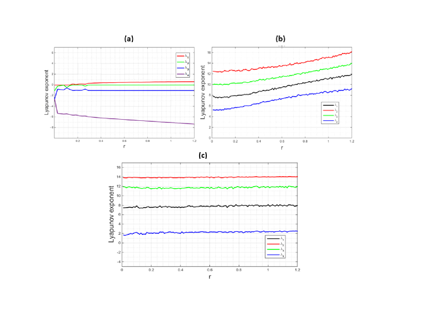
Figure 3: Lyapunov exponent values for: (a) Chaotic system in [6], (a) Case i, (b) Case ii.

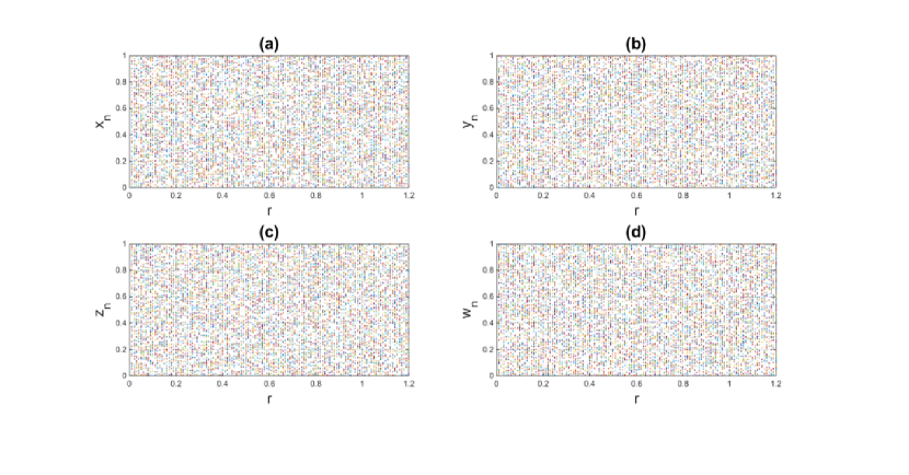
Figure 4: Bifurcation diagram results for the case i.

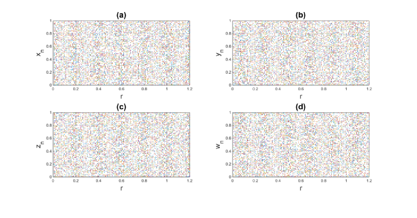
Figure 5: Bifurcation diagram results for the case ii.

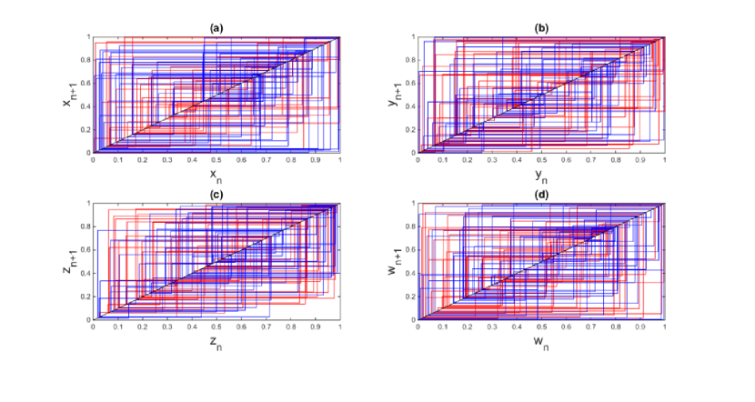
Figure 6: Cobweb plots for the case i.

Distribution is another important factor in evaluating chaotic system. One of the reasons for the weakness of chaos systems against the statistical attack is nonuniform distribution. The histogram plots of the proposed system for the case i are given in the Fig. 7. Also, the distribution patterns of the case ii are shown in Fig. 8. By using these results, it can be seen that the generated sequence of the proposed maps have flat distributions.

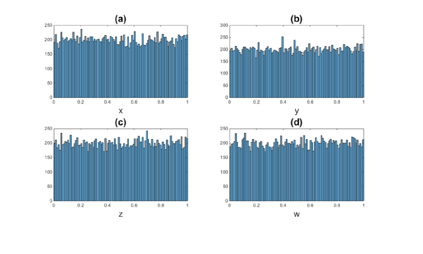
Figure 7: Histogram plots of the case i for r=0.5.

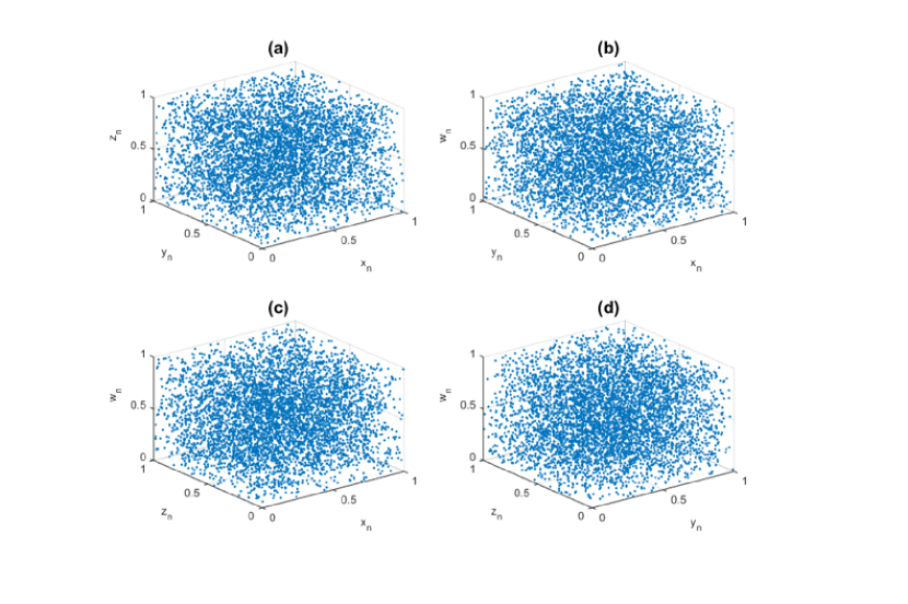
Figure 8: Distribution patterns of the case ii for $r=0.4$.

Remark 2.2.

In the continuation of this paper outputs of the proposed four-dimensional chaos system with initial values $\gamma=(x_{0},y_{0},z_{0},w_{0})$ and $r$ is shown by using the following notation

$${}^{\gamma}\Psi^{n}_{r}:=\left[{\begin{array}[]{*{20}{c}}{\begin{array}[]{*{20}{c}}{x_{1}}\\ {y_{1}}\\ {z_{1}}\\ {w_{1}}\\ \end{array}}&{\begin{array}[]{*{20}{c}}{x_{2}}\\ {y_{2}}\\ {z_{2}}\\ {w_{2}}\\ \end{array}}&{\begin{array}[]{*{20}{c}}{\cdots}\\ {\cdots}\\ {\cdots}\\ {\cdots}\\ \end{array}}&{\begin{array}[]{*{20}{c}}{x_{n}}\\ {y_{n}}\\ {z_{n}}\\ {w_{n}}\\ \end{array}}\\ \end{array}}\right].$$

Also ${}_{\tau}^{\gamma}\Psi^{n}_{r}$ denotes ${}^{\gamma}\Psi^{n}_{r}$, which the decimal part of the numbers is cut from the $\tau$-th decimal number to the next digits.

3 One and three dimensional shift Functions

In this section, we introduce two types of functions named $\operatorname{ULTS1D}$ and $\operatorname{S3D}$ to intermix pixels of images. The former is upper and lower triangular shift function which is suitable for grayscale images and the latter is suitable for RGB images. Note that applying these functions on images does not change the original image size and only the pixel locations are moved. In the continuation of this section, $n_{1},n_{2},n_{3},n_{4}$ are integers and $n,m$ are natural numbers which $m$ is divisible by 3 and $\frac{m}{3}$ is perfect square. $A,B$ and $C$ are matrices of size $n\times n$ and $P$ is a permutation of size $m$. The inputs of $\operatorname{ULTS1D}$ are $A$, $n_{1}$ and the output matrix $\operatorname{ULTS1D}(A,n_{1})$ is expressed as follows.

As seen in Figure 9, the pixel shuffling by $\operatorname{ULTS1D}$ starts from $A(1,1)$ entry and continues along the first row. Entries are shifted in the number of $n_{1}$ units. After reaching $A(1,n)$, it changes direction to the secondary diameter until it reaches $A(n,1)$. Upon reaching $A(n,1)$, entries keep on moving across the last row and last column, respectively. In $A(2,n)$, the route again change to diagonal, and this time along the sub-secondary diagonal. In this shift, there are some mutations of different lengths over secondary diameters that the first and shortest jump is from $A(n-1,3)$ to $A(n-1,1)$. After first jump, we move straight from bottom to top towards $A(2,1)$ and after entering this entry, we move towards $A(2,n-3)$. After a unit of diagonal movement, we enter the third row to traverse $A(3,2)$. Now we enter $A(4,2)$ and similarly continue the displacement of entries. Note that in this process, we do not enter a situation that we have already passed through, and as mentioned before, we make jumps wherever necessary.

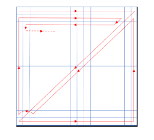
Figure 9: The path of one dimentional upper and lower triangular shift function ($\operatorname{ULTS1D}$).

Now, by applying composition of functions and the shift function defined above, we will introduce $\operatorname{FCS1D}$ and $\operatorname{SCS1D}$ functions. The outputs $B=\operatorname{FCS1D}(A,n_{1},n_{2},n_{3},n_{4})$ and $C=\operatorname{SCS1D}(A,n_{1},n_{2},n_{3},n_{4})$ are obtained as follow.

$B=\operatorname{ULTS1D}(A,n_{1})$;

$B=\operatorname{ULTS1D}(B^{\prime},n_{2})$;

$B=\operatorname{ULTS1D}\big{(}\operatorname{fliplr}(B),n_{3}\big{)}$

$B=\operatorname{ULTS1D}\big{(}\operatorname{flipud}(B),n_{4}\big{)}$;

$C=\operatorname{ULTS1D}\big{(}\operatorname{flipud}(A),n_{1}\big{)}$;

$C=\operatorname{ULTS1D}\big{(}\operatorname{fliplr}(C),n_{2}\big{)}$;

$C=\operatorname{ULTS1D}(C^{\prime},n_{3})$;

$C=\operatorname{ULTS1D}(C,n_{4})$;

which $B^{\prime}$ is transpose matrix of $B$. For better understanding, examples for one-dimensional shift functions are given in Fig 10.

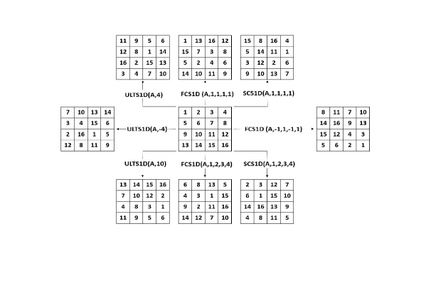
Figure 10: Examples for 1D shift functions.

In order to shuffle pixels of matrices $A,B$ and $C$ by swapping their parts based on $P$, we define three-dimensional shift function which is shown by $\operatorname{S3D}$. To get the output matrices of $\operatorname{S3D}(A,B,C,P)$, first, we block the matrices $A,B$ and $C$ to obtain the block matrices $\tilde{A},\tilde{B},\tilde{C}\in(\mathbb{R}^{p\times p})^{\frac{n}{p}\times\frac{n}{p}}$, which $p=\frac{n}{\sqrt{\frac{m}{3}}}$. Then, we convert these block matrices to block vectors $V\tilde{A},V\tilde{B},V\tilde{C}\in(\mathbb{R}^{p\times p})^{1\times\frac{n^{2}}{p^{2}}}$. Next, we consider the block vector $\tilde{V}=[V\tilde{A},V\tilde{B},V\tilde{C}]\in(\mathbb{R}^{p\times p})^{1\times\frac{3n^{2}}{p^{2}}}$. Now is the time to change the location of blocks of $\tilde{V}$ based on $P$ to get block vector $\tilde{W}\in(\mathbb{R}^{p\times p})^{1\times\frac{3n^{2}}{p^{2}}}$ as follow.

for j=1:$\operatorname{size}$($\tilde{V}$,2) do

     $\tilde{W}\{1,j\}=\tilde{V}\big{\{}1,P(1,j)\big{\}}$;

end for

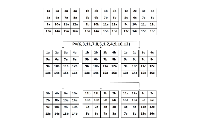
Figure 11: Example for the 3D shift function for $m=12$.

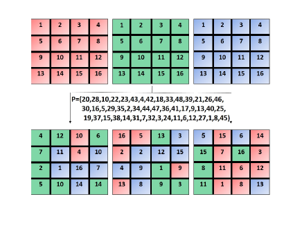
Figure 12: Example for the 3D shift function for $m=48$.

Also Fig 12 is the step of relocating blocks of block matrices for $m=48$. All the above operations are invertible and inverses of $\operatorname{FCS1D}$ and $\operatorname{SCS1D}$ and $\operatorname{S3D}$ are shown by $\operatorname{InvFCS1D}$ and $\operatorname{InvSCS1D}$ and $\operatorname{InvS3D}$, respectively.

4 Cellular Automata

The study of cellular automata(CA) dates back to Von.Neumonn [10]. CA is a model to describe a dynamic system composed of discrete cells where each cell can assume either the value $0$ or $1$. These cells create a lattice which changes in discrete time according local rules. Generally, a CA can be defined as $\{C,S,V,F\}$, where $C$ is the cell space and $S$ is the discrete state sets, like $\{0,1\}$. $V$ determines cellular neighborhoods and $F$ is transfer function[5, 19, 20]. CA are categorized in different dimensions [12] and the process of running one dimensional CA with local rule $30$ and triple neighborhoods are shown in Fig. 13. At this fig, 1 and 0 are shown with black and white squares, respectively, and $[0101110]$ is considered as the first input of CA. Eight possible states for $[0101110]$ with triple neighborhoods are shown in the second row. Third row shows the next state of cells. This process up to three steps, is shown in the last row of Fig. 13. Cellular automat ,which works based on simple logic computations, with pseudorandom hash behavior [13], is highly parallel and distributed systems that can simulate complicated behaviors [19]. One of the ways to create a strong cipher system is to use cellular automata with the large number of rules.

In our proposed algorithm, one-dimensional CA with triple neighborhoods is used like Fig. 13, which the rule number for each input is obtained based on proposed chaotic system.

Figure 13: (a) Cellular automata with rule number $30$, (b) Cellular automata process.

Remark 4.1.

The outputs of the decryption by reversible cellular automata is shown by

$$[\textbf{x}^{\prime},\textbf{y}^{\prime}]:=\Phi(\textbf{x},\textbf{y},rule,rep),$$

where x and y are inputs in the $t-1$ and $t$ times, respectively. ”$rule$” is the rule number after ”$rep$” repetitions.

In the proposed algorithm, the matrix $M_{n\times n}$ is encrypted based on reversible cellular automata by following algorithm.

$R=\big{[}{}_{2}^{\gamma}\Psi^{n/2}_{r}(1,:),{}_{2}^{\gamma}\Psi^{n/2}_{r}(2,:),{}_{2}^{\gamma}\Psi^{n/2}_{r}(3,:),{}_{2}^{\gamma}\Psi^{n/2}_{r}(4,:)\big{]}$;

for $i=1:n$ do

     if $i==1$ then

         $T=\operatorname{diag}(M,i)$;

         $X=T(1:n/2)$;

         $Y=T(n/2+1:n)$;

     else if $i!=1$ then

         $X=\operatorname{diag}(M,i)$;

         $Y=\operatorname{diag}(M,-i)$;

     end if

     $[\textbf{x},\textbf{y}]=\Phi(\textbf{x},\textbf{y},rule=R(i),1);$

end for

5 Proposed encryption algorithm

The details of the encryption algorithm are given in this section. The proposed algorithm includes two parts. In the first part a sensitive algorithm for generating key space is introduced and in the second part, an algorithm is proposed for image encryption.

5.1 Key space generation algorithm

In the process of encryption and decryption methods, the important part that affects the output of the algorithm is the key space. In this section, an algorithm to generate an efficient key space is introduced. One of the most important features of the proposed key space is the sensitivity to slight changes in input images, which is evaluated in the section related to simulation results. First, we design the proposed algorithm for image as follows.

Input: $I,r$;

$r_{0}=4\operatorname{rand}()$;

$r_{1}:=\lfloor r_{0}\times 10^{3}\rfloor$;

$I_{1}=\operatorname{circshift}\big{(}\operatorname{reshape}(I^{\prime},1,[]),r_{1}\big{)}$;

$\gamma_{0}:=I_{1}(1:4)$;

$q:=^{\gamma_{0}}\Psi^{1}_{r}$;

for $i=7:3:nm$ do

     $\gamma_{1}:=\Big{(}\operatorname{mean}\big{(}q(2:4)\big{)},q(1),I_{1}(i-2),I_{1}(i-1),I_{1}(i)\Big{)}$;

     $q=^{\gamma_{1}}\Psi^{1}_{r}$;

end for

output: $r_{0},q$;

This part of the algorithm is shown by the following notation according to the output and input values:

$$(r,r_{0},q)=\operatorname{key}(I,r).$$

For a color image $I_{n\times m\times 3}$, consider $I_{1}\in R^{n\times 3m}$ as follows.

$$I_{1}\big{(}1:n,(i-1)m+1:im\big{)}:=I(:,:,i),~{}~{}i=1,2,3.$$

Then define

$$I_{2}=\operatorname{circshift}\big{(}I_{1},\lfloor r_{0}\times 10^{3}\rfloor\big{)},$$

where $r_{0}:=4\operatorname{rand}()$. By using Algorithm 1, obtain

$$(r,r_{i},q_{i})=\operatorname{key}\Big{(}I_{2}\big{(}1:n,(i-1)m+1:im\big{)},r\Big{)},~{}~{}i=1,2,3.$$

In the last step of key generation for color image, consider key space as

$$(r_{0},q)=\Big{(}\operatorname{mean}\big{(}\{r_{i}\}^{3}_{i=1}\big{)},\operatorname{mean}\big{(}\{q_{i}\}^{3}_{i=1}\big{)}\Big{)}.$$

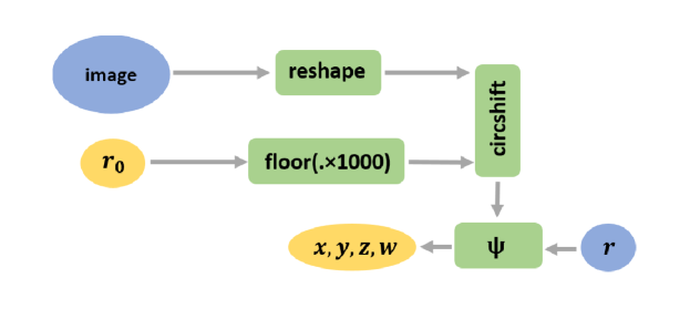
Figure 14: The structure of the proposed key generation algorithm.

5.2 Encryption and decryption algorithm

The steps of the proposed encryption algorithm for a grayscale image $I\in R^{n\times m}$ based on the new proposed chaos system are written as follows.

step 1. By using key space generation algorithm obtain:

$$(r,r_{0},q)=\operatorname{key}(I,r),$$

where $q=(x,y,z,w)$.

step 2. Define $\textbf{v}_{1}\in R^{1\times n}$, $\textbf{v}_{2}\in R^{1\times 8m}$ and $M\in R^{n\times m}$as

$$\textbf{v}_{1}:=\lfloor\chi^{n}_{r}\times 10^{3}\rfloor,$$

$$\textbf{v}_{2}:=\lfloor\chi^{8m}_{r_{0}}\times 10^{3}\rfloor,$$

$$M:=mod\Big{(}\big{\lfloor}\operatorname{reshape}\big{(}\chi^{nm}_{\operatorname{mean}([r,r_{0}])}\times 10^{3},[n,m]\big{)}\big{\rfloor},255\Big{)},$$

where

$$\chi^{j}_{r}=\big{[}^{q}\Psi^{\frac{j}{4}}_{r}(1,:),~{}~{}^{q}\Psi^{\frac{j}{4}}_{r}(2,:),~{}~{}^{q}\Psi^{\frac{j}{4}}_{r}(3,:),~{}~{}^{q}\Psi^{\frac{j}{4}}_{r}(4,:)\big{]},~{}~{}j=n,8m,nm.$$

step 3. Transfer $I$ to binary image $I_{1}\in R^{n\times 8m}$, and shift as

for i=1:n do

     $I_{1}(i,1:8m)=\operatorname{circshift}\Big{(}\big{(}I_{1}(i,1:8m)\big{)}^{\prime},\textbf{v}_{1}(i)\Big{)}^{\prime}$;

end for

for i=1:4 do

     $R\big{(}(i-1)n+1:2n,1:2m\big{)}=I_{1}\big{(}1:n,2(i-1)m+1:2im\big{)}$;

end for

for i=1:2m do

     $SR(1:4n,i)=\operatorname{circshift}\big{(}R(1:4n,i),\textbf{v}_{2}(i)\big{)}$;

end for

for i=1:4 do

     $I_{2}\big{(}1:n,2(i-1)m+1:2im\big{)}=SR\big{(}(i-1)n+1:in,1:2m\big{)}$;

end for

step 4. Consider most and least significant bits in two separate matrices $I_{2}^{m},I_{2}^{l}\in R^{n\times 4m}$, respectively. Then define $I_{3}\in R^{s\times 4m}$ with $s=n/2-mod(n/2,3)$ by

$$I_{3}=I^{m}_{2}(1:2:2s,:).$$

step 5. By using proposed algorithm based on cellular automata in Section 4, obtain $I_{4}$ for input values $I_{3},q$ and $r$.

step 6. By inverting steps 3 and 4 on $I_{4}$ obtain $I_{5}\in R^{n\times m}$ and shift $I_{5}$ as

$$I_{6}=\operatorname{FCS1D}\big{(}I_{5},\textbf{v}_{1}(10),-\textbf{v}_{1}(20),\textbf{v}_{1}(30),-\textbf{v}_{1}(40)\big{)}.$$

step 7. Obtain final encryption image $EI$ by using bitwise XOR operation as

$$EI=I_{6}\oplus M\oplus M_{s},$$

where $M_{s}:=\operatorname{circshift}\Big{(}M,\big{[}\lfloor q(1)\rfloor,\lfloor q(0)\rfloor\big{]}\times 10^{2}\Big{)}$.

Now, we develop the above proposed algorithm for color image $I\in R^{n\times m\times 3}$. In the first step, by using key space algorithm for color image obtain $(r,r_{0},q)$. Next by $\operatorname{S3D}$ shift function obtain $I_{1}$ as

$$\big{(}I_{1}(:,:,1),I_{1}(:,:,2),I_{1}(:,:,3)\big{)}=\operatorname{S3D}\big{(}I(:,:,1),I(:,:,2),I(:,:,3),p\big{)},$$

where $p=\operatorname{sort}(^{q}\Psi^{nm}_{r})$. Finally, each layer of $I_{1}$ is encrypted using the encryption algorithm that described above.
Decryption processes are achieved simply by following reverse steps of the above algorithms.

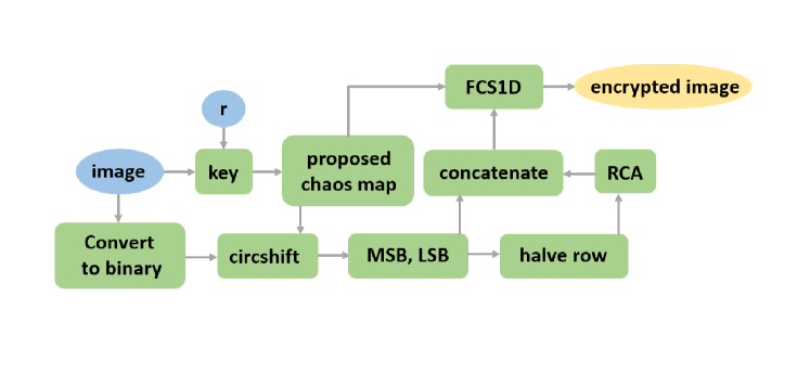
Figure 15: The structure of the proposed encryption algorithm.

6 Simulation results

In this section, we review the results of the algorithm and to check the security of the proposed algorithm, we perform different types of security tests.

6.1 Key space analysis

In order to show the sensitivity of the key generation algorithm to the input values, Table 1 shows the output results of the algorithm for different inputs. According to the results, it can be seen that small changes in the input of the algorithm have caused changes in the key space. To withstand the brute force attacks the key space must be large enough. According to [1], this size must be greater than $2^{100}$. If the precision computing is considered as $10^{-15}$, then the key space size is $10^{90}=2^{90log_{2}10}\approx 2^{298}$, and this is large enough to resist the attack.

Table 1: Key space generated by the proposed algorithm for various inputs and $r=0.7$.

		Keys
Image		$r_{0}$	$x$	$y$	$z$	$w$
lena	Original	constant(0.7)	0.6038	0.2828	0.7086	0.4590
$(256\times 256\times 3)$	One bit changed	constant(0.7)	0.5495	0.3590	0.9294	0.3930
	Original	random	0.6600	0.7191	0.3064	0.8206
	One bit changed	random	0.4336	0.4298	0.2942	0.4056
	First time run	random	0.2499	0.4357	0.5456	0.5322
	Second time run	random	0.4351	0.2396	0.6711	0.5193
lena	Original	constant(0.7)	0.7753	0.3087	0.5087	0.1720
$(256\times 256)$	One bit changed	constant(0.7)	0.6800	0.6547	0.2556	0.3093
	Original	random	0.8145	0.4966	0.3931	0.0714
	One bit changed	random	0.0451	0.4445	0.0295	0.7943
pirate	Original	constant(0.7)	0.3329	0.9476	0.2881	0.5595
$(256\times 256)$	First pixel changed	constant(0.7)	0.8755	0.1108	0.6811	0.4796
	Last pixel changed	constant(0.7)	0.3318	0.6714	0.1125	0.6366
	Original	random	0.8654	0.2863	0.0157	0.5612
	First pixel changed	random	0.7584	0.9722	0.1689	0.9224
	Last pixel changed	random	0.7952	0.4099	0.1525	0.0080

6.2 Statistical analysis

Statistical test consists of three basic tests, correlation values, information entropy and histogram analysis. The correlation values for an image are calculated using the following formula

$$C_{x,y}=\frac{E(x-\bar{x})(y-\bar{y})}{\sigma_{x}\sigma_{y}},$$

where $E,\bar{x},\bar{y},\sigma_{x}$ and $\sigma_{y}$ represent expectation, mean values and standard deviation, respectively. If this number is close to zero, the encrypted image will not have significant information from the original image. The results of this value for original and encrypted image are give in Tables 2 and 3. By comparing values of encrypted and original images, it is observed that the results for the encrypted images are close to the ideal value, i.e., zero. Also the correlation distributions for the original and encrypted images are shown in Figures 16-18. By using these figures, it can be seen that encrypted images have more uniform distribution.

Table 2: Correlation coefficient and Information entropy values in the plain and cipher grayscale images.

	Correlation coefficient				Information
	Horizontal	Vertical	Diagonal	Diagonal	entropy
			(lower left to top right)	(lower right to top left)
plain images
5.1.12	0.95649	0.97408	0.93627	0.93893	6.7057
5.2.08	0.93707	0.89264	0.85427	0.85572	7.201
boat($512\times 512$)	0.93812	0.97131	0.92585	0.92216	7.1914
lena($256\times 256$)	0.92578	0.95926	0.92577	0.90374	7.4429
lena($512\times 512$)	0.20131	0.21056	0.19815	0.19016	7.4455
encrypted images
5.1.12	$-0.00047766$	$0.00061399$	$0.001538$	$-0.0001677$	7.9973
5.2.08	$-0.0003788$	0.00013229	$-0.00082042$	$0.00027628$	7.9993
boat($512\times 512$)	0.00093687	0.00057866	0.00038615	$-0.00084275$	7.9993
lena($256\times 256$)	$-0.0021188$	$-0.0025797$	$-0.0015225$	0.00026687	7.9972
lena($512\times 512$)	0.00039856	0.00015902	$-0.00023439$	$0.00069882$	7.9993

Table 3: Correlation coefficient values in the plain and cipher grayscale images.

		Correlation coefficient				Information
		Horizontal	Vertical	Diagonal	Diagonal	entropy
				(lower left to top right)	(lower right to top left)
plain images
	R	0.94928	0.95616	0.91631	0.91764	6.2499
4.1.02	G	0.93077	0.95338	0.8968	0.90017	5.9642
	B	0.91784	0.94421	0.88698	0.88898	5.9309
	R	0.97865	0.9879	0.96875	0.96841	7.2549
4.1.04	G	0.96598	0.98201	0.95147	0.95072	7.2704
	B	0.95231	0.97178	0.93069	0.93057	6.7825
	R	0.92307	0.86596	0.85187	0.85434	7.7067
4.2.03	G	0.86548	0.76501	0.72493	0.7348	7.4744
	B	0.90734	0.88089	0.84244	0.83986	7.7522
	R	0.97527	0.98531	0.97339	0.96484	5.0465
lena	G	0.96662	0.98017	0.96303	0.95357	5.4576
($512\times 512\times 3$)	B	0.93339	0.95579	0.92643	0.91863	4.8001
encrypted images
	R	0.0011619	0.0016396	0.00053731	0.00082608	7.9973
4.1.02	G	0.0007757	$-0.00021986$	0.00069429	0.00088685	7.9971
	B	0.00029618	0.0005109	0.00098397	$-0.0015792$	7.9972
	R	0.00036129	$-0.00047313$	-0.0015582	0.0026443	7.9973
4.1.04	G	0.0029232	0.0014998	0.0010652	0.001758	7.9972
	B	0.0031419	0.00095978	0.0019824	$-0.001847$	7.9973
	R	$-0.00057646$	0.00020068	0.0010341	$-0.00034744$	7.9993
4.2.03	G	0.00053615	$-0.00029491$	0.00061376	$-0.00040553$	7.9993
	B	$-0.00080725$	$-0.0017738$	$-0.0002713$	0.0009324	7.9993
	R	$-2.2351e-06$	0.00022357	$-0.00074232$	$-0.00055947$	7.9993
lena	G	0.0002728	$-3.7743e-05$	0.0012758	$-0.00036377$	7.9993
($512\times 512\times 3$)	B	0.00031603	$0.00067082$	$-0.00071107$	0.0012129	7.9993

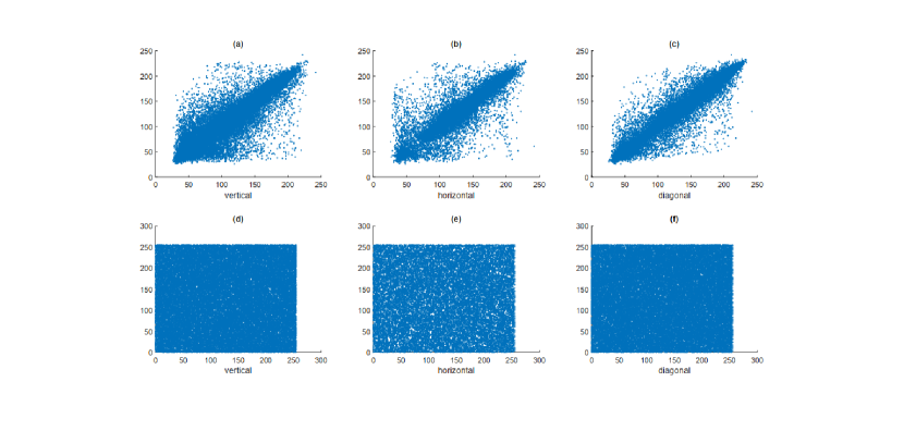
Figure 16: Correlation of neighborhood pixels at different directions before (a-c) and after encryption (d-f) of lena ($256\times 256$).

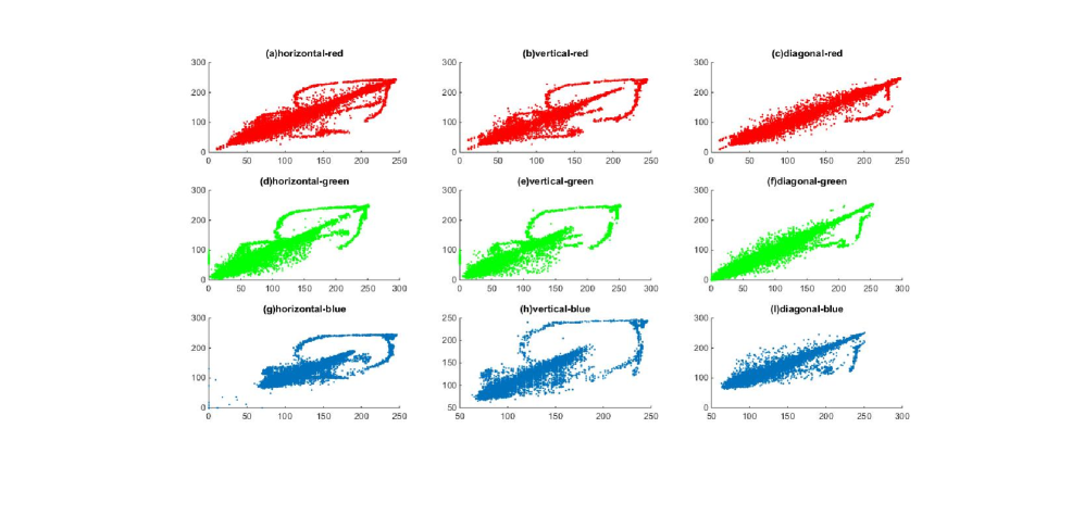
Figure 17: Correlation of neighborhood pixels at different directions for 4.1.04.

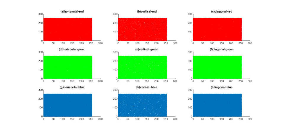
Figure 18: Correlation of neighborhood pixels at different directions for encrypted 4.1.04

The uncertainty of information for an image is evaluated by using Shannon information entropy. This value is calculated by

$$H=-\sum_{i}p(i)\log\big{(}p(i)\big{)},$$

where $p(i)$ is the probability of occurrence of each pixel. The ideal value for this test is 8. If the results of the algorithm are close to this number, it will be difficult to obtain valid information from the image. The results of this test for different images with different sizes are given in Tables 2 and 3. The results in these tables show that the information entropy of encrypted image by proposed algorithm are close to the ideal value. The distribution characteristics of pixel values is evaluated by histogram. Histograms of plaintext and encrypted images are given in Figure 19. Also the intensity histogram is shown in Figure 20. Using these results, it can be seen that the histograms of the cipher image are uniformly distributed in comparison with the original image. Therefore, according to the results the proposed algorithm has a good ability to resist statistical attacks.

6.3 Differential attack test

One of the most important attacks evaluated on cryptographic algorithms is differential attacks. This type of attack is studied by two tests, UACR test (number of pixels change rate) and NPCI test (unified average changing intensity). These values are calculated by

$$NPCR=\frac{\sum_{i,j}D_{i,j}}{n\times m}\times 100\%,$$

$$UACI=\frac{\sum_{i,j}|C^{1}_{i,j}-C^{2}_{i,j}|}{n\times m}\times 100\%,$$

where $C^{1}$ and $C^{2}$ are two encrypted images such that their plain images differ only by one pixel. Also if $C^{1}_{i,j}\neq C^{2}_{i,j}$ then $D_{i,j}=1$ otherwise $D_{i,j}=0$. The ideal values for these tests are $100\%$ and $33.\overline{33}\%$, respectively. The results are shown in Tables 4-6. The best study on these values is discussed in [22], which critical intervals for NPCR and UACI are considered. In Tables 4 and 5, the results of the proposed algorithm for different images are compared to the critical values. These results indicate the success of the proposed method in these tests. Also in Table 6, the proposed method are compared to other studies.

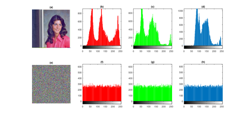
Figure 19: (a)-(d) the original image and its histogram, (e)-(f) the output image of the proposed algorithm and its histogram

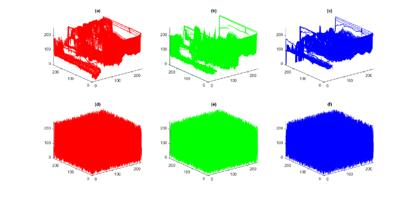
Figure 20: (a)-(c) 3D histogram representation of original image and (d)-(f) encrypted image for 4.1.04.

Table 4: Numerical results of the UACI and NPCR for different images ($256\times 256$).

			UACI critical values [22]				NPCR critical values [22]
			u${}^{*-}_{0.05}$=33.2824	u${}^{*-}_{0.01}$=33.2255	u${}^{*-}_{0.001}$=33.1594		N${}^{*}_{0.05}=$	N${}^{*}_{0.01}=$	N${}^{*+}_{0.001}=$
Image		UACI	u${}^{*+}_{0.05}$=33.6447	u${}^{*+}_{0.01}$=33.7016	u${}^{*+}_{0.001}$=33.7677	NPCR	99.5693	99.5527	99.5341
5.1.12		33.4570	Pass	Pass	Pass	99.6127	Pass	Pass	Pass
lena		33.4931	Pass	Pass	Pass	99.6112	Pass	Pass	Pass
	R	33.4931	Pass	Pass	Pass	99.6213	Pass	Pass	Pass
4.1.02	G	33.4763	Pass	Pass	Pass	99.6000	Pass	Pass	Pass
	B	33.4421	Pass	Pass	Pass	99.6147	Pass	Pass	Pass
	R	33.4882	Pass	Pass	Pass	99.6191	Pass	Pass	Pass
4.1.04	G	33.4581	Pass	Pass	Pass	99.6032	Pass	Pass	Pass
	B	33.5000	Pass	Pass	Pass	99.6001	Pass	Pass	Pass

Table 5: Numerical results of the UACI and NPCR for different images ($512\times 512$).

			UACI critical values [22]				NPCR critical values[22]
			u${}^{*-}_{0.05}$=33.3730	u${}^{*-}_{0.01}$=33.3445	u${}^{*-}_{0.001}$=33.3115		N${}^{*}_{0.05}=$	N${}^{*}_{0.01}=$	N${}^{*+}_{0.001}=$
Image		UACI	u${}^{*+}_{0.05}$=33.5541	u${}^{*+}_{0.01}$=33.5826	u${}^{*+}_{0.001}$=33.6156	NPCR	99.5893	99.5810	99.5717
5.2.08		33.4571	Pass	Pass	Pass	99.6115	Pass	Pass	Pass
boat		33.4750	Pass	Pass	Pass	99.6137	Pass	Pass	Pass
lena		33.4683	Pass	Pass	Pass	99.6046	Pass	Pass	Pass
	R	33.4546	Pass	Pass	Pass	99.6215	Pass	Pass	Pass
4.2.03	G	33.4681	Pass	Pass	Pass	99.6064	Pass	Pass	Pass
	B	33.4502	Pass	Pass	Pass	99.6110	Pass	Pass	Pass
	R	33.4641	Pass	Pass	Pass	99.6112	Pass	Pass	Pass
lena	G	33.4541	Pass	Pass	Pass	99.6080	Pass	Pass	Pass
	B	33.4543	Pass	Pass	Pass	99.6101	Pass	Pass	Pass

Table 6: Correlation coefficient and Information entropy values in the plain and cipher grayscale images.

	NPCR				UACI
image	Propose	Ref.[15]	Ref.[18]	Ref.[6]		Propose	Ref.[15]	Ref.[18]	Ref.[6]
5.1.09	99.6117	99.6078	99.6016	99.6064		33.4490	33.4563	33.4700	33.4456
5.1.10	99.6164	99.6098	99.6191	99.6154		33.4733	33.4510	33.4826	33.4946
5.1.11	99.6122	99.6077	99.6042	99.6244		33.4654	33.4832	33.5648	33.5541
5.1.14	99.6118	99.6129	99.6199	99.6364		33.5111	33.4848	33.4725	33.4655
7.1.01	99.6161	99.6040	99.6053	99.5992		33.4682	33.4779	33.4820	33.5037
7.1.02	99.6093	99.6016	99.6080	99.6075		33.4730	33.4172	33.4357	33.4237
7.1.09	99.6152	99.6061	99.6112	99.6162		33.4591	33.4814	33.4596	33.4177
7.1.10	99.6110	99.6052	99.6106	99.6045		33.4817	33.4852	33.4538	33.4344

6.4 Noise and data loss attack

In the transmission of images over the network and through physical channels, part of the data is naturally or intentionally lost due to noise and cropped attacks. Therefore, efficient cryptographic schemes are capable of retrieving the original images even after these types of attacks. In order to test the anti-noise ability of the proposed method, the decrypted images after the noise attack with different intensities $0.1$ for gray and $0.2$ for color images are given in Fig.21. The strength of the proposed method against cropped attacks with varying degrees of data loss is shown in Fig.22.

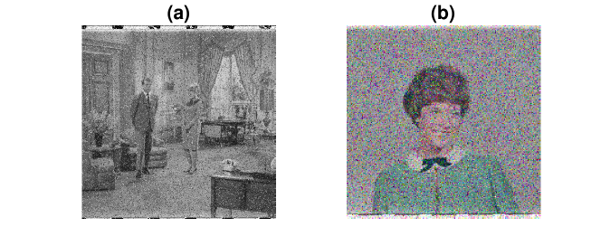
Figure 21: Salt $\&$ pepper noise attack results with different noise density and extracted secret images: (a), (d) decrypted images with noise intensity 0.1 and 0.2, respectively.

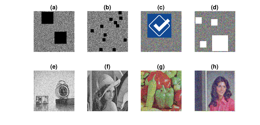
Figure 22: Results of extracting the secret image after slight change in the key: (a) almost 0.17 data loss, (b) almost 0.07 data loss, (c) almost 0.35 data loss, (d) almost 0.23 data loss, (e)-(h) decrypted images.

7 Conclusions

Create a secure environment for transferring images a burgeoning subject branch. To study this topic, in the first step, by the development and improvement of the chaos system, a new chaos system is introduced. The structure of the new system is studied with different tests and the results show the efficiency of the new system. In the next step, the proposed system is used to create a secure image transfer environment in the form of an encryption algorithm. The results of studying the proposed algorithm by various security tests show that the proposed algorithm is efficient and safe.

Funding This work does not receive any funding.

Compliance with ethical standards

Conflict of interests The authors declare that they have no conflict of interests.
Human participants and animals This paper does not include human participants and animals.

References

- [1] Alvarez, G. and Li, S., 2006. Some basic cryptographic requirements for chaos-based cryptosystems. International journal of bifurcation and chaos, 16(08), pp.2129-2151.
- [2] Del Rey, A.M. and Sánchez, G.R., 2015. An image encryption algorithm based on 3D cellular automata and chaotic maps. International Journal of Modern Physics C, 26(01), p.1450069.
- [3] Dmitrieva, L.A., Kuperin, Y.A., Smetanin, N.M. and Chernykh, G.A., 2016, June. Method of calculating Lyapunov exponents for time series using artificial neural networks committees. In 2016 Days on Diffraction (DD) (pp. 127-132). IEEE.
- [4] Fridrich, J., 2009. Steganography in digital media: principles, algorithms, and applications. Cambridge University Press.
- [5] Gutowitz, H. ed., 1991. Cellular automata: Theory and experiment. MIT press.
- [6] Hua, Z., Zhou, Y. and Huang, H., 2019. Cosine-transform-based chaotic system for image encryption. Information Sciences, 480, pp.403-419.
- [7] Lynch, S., 2004. Dynamical systems with applications using MATLAB. Boston: Birkhäuser.
- [8] Naskar, P.K., Bhattacharyya, S., Nandy, D. and Chaudhuri, A., 2020. A robust image encryption scheme using chaotic tent map and cellular automata. Nonlinear Dynamics, 100(3), pp.2877-2898.
- [9] Natiq, H., Said, M.R.M., Al-Saidi, N.M. and Kilicman, A., 2019. Dynamics and complexity of a new 4d chaotic laser system. Entropy, 21(1), p.34.
- [10] Neumann, J. and Burks, A.W., 1966. Theory of self-reproducing automata (Vol. 1102024). Urbana: University of Illinois press.
- [11] Sano, M. and Sawada, Y., 1985. Measurement of the Lyapunov spectrum from a chaotic time series. Physical review letters, 55(10), p.1082.
- [12] Sarkar, P., 2000. A brief history of cellular automata. Acm computing surveys (csur), 32(1), pp.80-107.
- [13] Sen, S., Shaw, C., Chowdhuri, D.R., Ganguly, N. and Chaudhuri, P.P., 2002, December. Cellular automata based cryptosystem (CAC). In International Conference on Information and Communications Security (pp. 303-314). Springer, Berlin, Heidelberg.
- [14] Van Opstall, M., 1998. Quantifying chaos in dynamical systems with Lyapunov exponents. Furman University Electronic Journal of Undergraduate Mathematics, 4(1), pp.1-8.
- [15] Wang, R., Deng, G.Q. and Duan, X.F., 2021. An image encryption scheme based on double chaotic cyclic shift and Josephus problem. Journal of Information Security and Applications, 58, p.102699.
- [16] Wang, X. and Guan, N., 2020. Chaotic image encryption algorithm based on block theory and reversible mixed cellular automata. Optics Laser Technology, 132, p.106501.
- [17] Wang, X. and Luan, D., 2013. A novel image encryption algorithm using chaos and reversible cellular automata. Communications in Nonlinear Science and Numerical Simulation, 18(11), pp.3075-3085.
- [18] Wang, X., Wang, Q. and Zhang, Y., 2015. A fast image algorithm based on rows and columns switch. Nonlinear Dynamics, 79(2), pp.1141-1149.
- [19] Wolfram, S., 1983. Statistical mechanics of cellular automata. Reviews of modern physics, 55(3), p.601.
- [20] Wolfram, S., 1986. Random sequence generation by cellular automata. Advances in applied mathematics, 7(2), pp.123-169.
- [21] Wolf, A., Swift, J.B., Swinney, H.L. and Vastano, J.A., 1985. Determining Lyapunov exponents from a time series. Physica D: nonlinear phenomena, 16(3), pp.285-317.
- [22] Wu, Y., Noonan, J.P. and Agaian, S., 2011. NPCR and UACI randomness tests for image encryption. Cyber journals: multidisciplinary journals in science and technology, Journal of Selected Areas in Telecommunications (JSAT), 1(2), pp.31-38.
- [23] Xie, E.Y., Li, C., Yu, S. and Lü, J., 2017. On the cryptanalysis of Fridrich’s chaotic image encryption scheme. Signal processing, 132, pp.150-154.
- [24] Zhang, H., Wang, X.Q., Sun, Y.J. and Wang, X.Y., 2020. A novel method for lossless image compression and encryption based on LWT, SPIHT and cellular automata. Signal Processing: Image Communication, 84, p.115829.