Singlet fermion dark matter and Dirac neutrinos from Peccei-Quinn symmetry

Abstract

The Peccei-Quinn (PQ) mechanism not only acts as an explanation for the absence of strong CP violation but also can play a main role in the solution to other open questions in particle physics and cosmology. Here we consider a model that identifies the PQ symmetry as a common thread in the solution to the strong CP problem, the generation of radiative Dirac neutrino masses and the origin of a multicomponent dark sector. Specifically, scotogenic neutrino masses arise at one loop level with the lightest fermionic mediator field acting as the second dark matter (DM) candidate thanks to the residual $Z_{2}$ symmetry resulting from the PQ symmetry breaking. We perform a phenomenological analysis addressing the constraints coming from the direct searches of DM, neutrino oscillation data and charged lepton flavor violating (LFV) processes. We find that the model can be partially probed in future facilities searching for WIMPs and axions, and accommodates rates for rare leptonic decays that are within the expected sensitivity of upcoming LFV experiments.

I Introduction

The apparent non-observation of CP violation in the QCD Lagrangian represents one of the most active subjects in high energy physics, both theoretical and experimentally speaking. In the theory side, the absence of strong CP violation can be dynamically explained invoking the Peccei-Quinn (PQ) mechanism Peccei:1977hh , which considers the spontaneous breaking of an anomalous global $U(1)$ symmetry with the associated pseudo-Nambu-Goldstone boson, the (QCD) axion Weinberg:1977ma ; Wilczek:1977pj . The axion itself turns to be a promising candidate for making up the dark matter (DM) of the Universe thanks to a variety of production mechanisms Sikivie:2006ni , for instance via the vacuum misalignment mechanism Preskill:1982cy ; Abbott:1982af ; Dine:1982ah . Besides this, it is remarkable that the physics behind the PQ mechanism can be also used to address other open questions in particle physics and cosmology such as neutrino masses Mohapatra:1982tc ; Shafi:1984ek ; Langacker:1986rj ; Shin:1987xc ; He:1988dm ; Berezhiani:1989fp ; Bertolini:1990vz ; Ma:2001ac , baryon asymmetry Servant:2014bla ; Ipek:2018lhm ; Croon:2019ugf ; Co:2019wyp and inflation Linde:1991km ; Folkerts:2013tua ; Fairbairn:2014zta ; Ballesteros:2016euj .

The recent analysis Carvajal:2018ohk considering the PQ mechanism as the responsible for the massiveness of neutrinos revealed that it is also possible to consistently accommodate radiative Dirac neutrino masses with a viable WIMP DM candidate, thus providing a set of multicomponent scotogenic models with Dirac neutrinos. Concretely, in these scenarios one-loop Dirac neutrino masses are generated through the $d=5$ effective operator $\bar{L}\tilde{H}N_{R}S$ Ma:2016mwh ; Yao:2018ekp once the axionic field $S$ develops a vacuum expectation value, with the contributions arising from the tree-level realizations of such an operator being forbidden thanks to the charge assignment. As a further consequence of the PQ symmetry, the residual discrete symmetry that is left over renders stable the lightest particle mediating the neutrino masses, and since such a particle must be electrically neutral, it turns out that the setup also accommodates a second DM species Baer:2011hx ; Bae:2013hma ; Dasgupta:2013cwa ; Alves:2016bib ; Ma:2017zyb ; Chatterjee:2018mac .

In this work we perform a phenomenological analysis of the T3-1-A-I model introduced in Ref. Carvajal:2018ohk . In order to determine the viable parameter space of the model we take into account the constraints coming from direct detection experiments, lepton flavor violation (LFV) processes, DM relic density and neutrino physics. We find that for a wide and typical range of the parameter values, the model easily satisfies these constraints and, additionally, future experiments will be able to test a considerable portion of the parameter space.

The layout of this paper is organized as follows. The main features of the model are presented in Section II. In Section III we determine the elastic scattering cross section between the WIMP particle and nucleons, and estimate the expected number of events in current and future direct detection experiments. Section IV is dedicated to a numerical analysis addressing the DM and LFV phenomenology. Finally, we conclude in Section V.

II The model

	$L_{\beta}$	$\ell_{R\beta}$	$N_{R\beta}$	$S$	$\psi_{i}$	$\Phi$	$H_{2}$	$D_{L}$	$D_{R}$
$U(1)_{L}$	$1$	$1$	$1$	$0$	$1$	$0$	$0$	$0$	$0$
$U(1)_{\textrm{PQ}}$	$2$	$2$	$0$	$2$	$3$	$3$	$1$	$1$	$-1$
$Z_{2}$	$+$	$+$	$+$	$+$	$-$	$-$	$-$	$-$	$-$

Table 1: Lepton number and PQ charge assignments for the model particles. Here, both the SM Higgs, $H_{1}$, and the ordinary quarks are even under the discrete symmetry and neutral under the global ones. The transformation properties under the remnant $Z_{2}$ symmetry are also shown. $\beta$ is a family index ($\beta=1,2,3)$ and $i=1,2$.

As usual in models with massive Dirac neutrinos, this model extends the SM with three singlet Weyl fermions $N_{R\beta}\,(\beta=1,2,3)$ $-$the right-handed partners of the SM neutrinos. The one-loop neutrino mass generation additionally demands Carvajal:2018ohk the introduction of one $SU(2)_{L}$ doublet scalar $H_{2}$, one singlet scalar $\Phi$ and two singlet Dirac fermions $\psi_{i}\,(i=1,2)$. As the last piece we have a chiral exotic down-type quark $D$ which is added in order to realize the hadronic KSVZ-type axion model Kim:1979if ; Shifman:1979if . In Table 1 are displayed the charge assignments under the $U(1)_{L}$ and $U(1)_{PQ}$ global symmetries, as well as under the remnant $Z_{2}$ symmetry. Notice that under this discrete symmetry the mediator fields in the neutrino mass diagram are odd, which implies that the lightest of them can be considered as a (WIMP-like) DM candidate.

The relevant part of the scalar potential can be expressed as

$$\mathcal{V} \supset-\mu_{1}^{2}|H_{1}|^{2}+\lambda_{1}|H_{1}|^{4}+\mu^{2}_{S}|S|^{2}+\lambda_{S}|S|^{4}+\mu^{2}_{2}|H_{2}|^{2}+\lambda_{2}|H_{2}|^{4}+\lambda_{3}|H_{1}|^{2}|H_{2}|^{2}+\lambda_{4}|H_{1}^{\dagger}H_{2}|^{2}$$

$$\,+\mu^{2}_{\Phi}|\Phi|^{2}+\lambda_{\Phi}|\Phi|^{4}+\lambda_{h\Phi}|H_{1}|^{2}|\Phi|^{2}+\lambda^{\prime}\left(\Phi^{*}S\tilde{H}_{2}^{\dagger}\tilde{H}_{1}+\textrm{h.c.}\right),$$ (1)

where the coupling constants associated to the quartic interaction terms $|\Phi|^{2}|S|^{2}$, $|H_{2}|^{2}|S|^{2}$, $|H_{2}|^{2}|\Phi|^{2}$ and $|H_{1}|^{2}|S|^{2}$ have been assumed to be small. Since the $(H_{1}^{\dagger}H_{2})^{2}+(H_{2}^{\dagger}H_{1})^{2}$ term is forbidden, it follows that the neutral component of $H_{2}$ remains as a complex field and does not get splitted into a CP-even and a CP-odd field. Nevertheless, it does get mixed with $\Phi$ through the term proportional to $\lambda^{\prime}$ (since both scalar fields do not acquire a nonzero vacuum expectation value). We parametrize the scalar fields as

$$S=\frac{1}{\sqrt{2}}\left(\rho+v_{S}\right)e^{ia/v_{S}},\hskip 14.22636ptH_{1}=\begin{pmatrix}0\\ \frac{v_{\textrm{SM}}+h}{\sqrt{2}}\end{pmatrix},\hskip 14.22636ptH_{2}=\begin{pmatrix}H^{+}\\ H^{0}\end{pmatrix},$$ (2)

where $\rho$ stands for the radial component of the field $S$ whose mass is set by the scale of the PQ symmetry breaking $v_{S}$, whereas the angular part of $S$ corresponds to the QCD axion $a$, $h$ is the SM Higgs boson and $v_{\textrm{SM}}=246.22$ GeV.

In the basis $(H^{0},\Phi)$, the mass matrix for the $Z_{2}$-odd neutral scalars

$$\mathcal{M}_{0}=\left(\begin{array}[]{cc}\mu_{2}^{2}+\frac{1}{2}(\lambda_{3}+\lambda_{4})v_{\textrm{SM}}^{2}&\frac{1}{2}\lambda^{\prime}v_{S}v_{\textrm{SM}}\\ \frac{1}{2}\lambda^{\prime}v_{S}v_{\textrm{SM}}&\mu_{\Phi}^{2}+\frac{1}{2}\lambda_{h\Phi}v_{\textrm{SM}}^{2}\end{array}\right),$$ (3)

leads to the mass eigenstates $S_{1,2}$ (both with two degrees of freedom since they are complex) via the transformation

$$H^{0} =\cos\varphi\ S_{1}+\sin\varphi\ S_{2}=\sum_{j=1,2}C_{Hj}S_{j}\equiv C_{Hj}S_{j},$$ (4)

$$\Phi =-\sin\varphi\ S_{1}+\cos\varphi\ S_{2}=\sum_{j=1,2}C_{\Phi j}S_{j}\equiv C_{\Phi j}S_{j},$$ (5)

where we have defined $C_{H1}=\cos\varphi,\,C_{H2}=\sin\varphi,\,C_{\Phi 1}=-\sin\varphi$ and $C_{\Phi 2}=\cos\varphi$. The mixing angle is defined through the expression

$$\sin(2\varphi)=\frac{\lambda^{\prime}v_{\textrm{SM}}v_{S}}{m^{2}_{S_{2}}-m^{2}_{S_{1}}},$$ (6)

being $m_{S_{1,2}}$ the eigenvalues of $\mathcal{M}_{0}$. In our analysis we will take $m_{S_{1}}<m_{S_{2}}$, which implies that for $\varphi\to 0$ the heavier scalar is mainly singlet, whereas for $\varphi\to\pm\,\pi/2$ the heavier one is mainly doublet. For the charged scalar $H^{\pm}$ we find that its mass is given by $m^{2}_{H^{\pm}}=\mu_{2}^{2}+\frac{1}{2}\lambda_{3}v_{\textrm{SM}}^{2}$, just as happens in the inert doublet model.

II.1 Neutrino masses and charged LFV

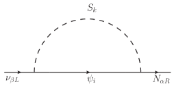
Figure 1: One-loop Feynman diagram leading to Dirac neutrino masses. The loop mediators are the singlet fermions $\psi_{1,2}$ and the neutral scalars $S_{1,2}$.

The new Yukawa interactions involving the SM leptons are given by

$$\mathcal{L}_{Y} =y_{i\beta}\overline{\psi_{i}}\tilde{H}_{2}^{\dagger}L_{\beta}+h_{\beta i}\Phi^{*}\overline{N_{R\beta}}\psi_{i}+\textrm{h.c.},$$ (7)

where $y_{i\beta}$ and $h_{\beta i}$ are $2\times 3$ and $3\times 2$ Yukawa matrices, respectively. After the spontaneous symmetry breaking, scotogenic Dirac neutrino masses are generated at one loop Farzan:2012sa ; Ma:2016mwh ; Wang:2016lve ; Borah:2016zbd ; Wang:2017mcy ; Yao:2017vtm ; Yao:2018ekp ; Ma:2017kgb ; Wang:2017mcy ; Reig:2018mdk ; Calle:2018ovc ; Calle:2019mxn ; Bernal:2021ezl as is illustrated in Fig. 1. The effective mass matrix can be written as

$$\big{(}M_{\nu}\big{)}_{\alpha\beta}=\sum_{i}h_{\alpha i}y_{i\beta}\kappa_{i},$$ (8)

where

$$\kappa_{i}=\frac{\sin(2\varphi)}{32\pi^{2}}m_{\psi_{i}}\left[F\left(\frac{m_{S_{2}}^{2}}{m_{\psi_{i}}^{2}}\right)-F\left(\frac{m_{S_{1}}^{2}}{m_{\psi_{i}}^{2}}\right)\right],$$ (9)

and $F(x)=x\ln(x)/(x-1)$. The Dirac neutrino mass matrix $M_{\nu}$ can be diagonalized through $M_{\nu}=VM^{diag}_{\nu}U^{\dagger}$, where $U$ and $V$ are unitary matrices and $M^{diag}_{\nu}$ is a diagonal mass matrix containing, in general, three mass eigenvalues different from zero. However, due to the flavor structure of $M_{\nu}$ only two neutrinos are massive (det$(M_{\nu})=0$). In the basis where the charged lepton mass matrix is diagonal the $U$ unitary matrix can be identified with the PMNS matrix Zyla:2020zbs , whereas $V$ can be assumed diagonal without loss of generality. This allows us to express the $y$ Yukawa couplings in terms of the $h$ ones. In the case of the normal neutrino mass hierarchy (NH)

$$y_{1\beta} =\frac{h_{32}m_{2}U^{*}_{\beta 2}-h_{22}m_{3}U^{*}_{\beta 3}}{(h_{21}h_{32}-h_{31}h_{22})k_{1}}\,,$$

$$y_{2\beta} =\frac{h_{21}m_{3}U^{*}_{\beta 3}-h_{31}m_{2}U^{*}_{\beta 2}}{(h_{21}h_{32}-h_{31}h_{22})k_{2}}\,,$$ (10)

with $h_{11}=h_{12}=0$, whereas in the inverted hierarchy (IH) case

$$y_{1\beta} =\frac{h_{12}m_{2}U^{*}_{\beta 2}-h_{22}m_{3}U^{*}_{\beta 1}}{(h_{12}h_{21}-h_{11}h_{22})k_{1}}\,,$$

$$y_{2\beta} =\frac{h_{21}m_{3}U^{*}_{\beta 1}-h_{11}m_{2}U^{*}_{\beta 2}}{(h_{12}h_{21}-h_{11}h_{22})k_{2}}\,,$$ (11)

with $h_{31}=h_{32}=0$. Notice that one of the right-handed neutrinos becomes decoupled because we are considering a scenario with the minimal set of singlet fermions.

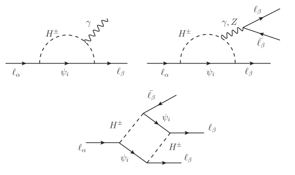
Figure 2: Feynman diagrams for the $\ell_{\alpha}\rightarrow\ell_{\beta}\gamma$ and $\ell_{\alpha}\rightarrow\ell_{\beta}\bar{\ell}_{\beta}\ell_{\beta}$ charged LFV processes present in the model.

Although Diracness of neutrino masses is compatible with the conservation of the total lepton number, family lepton number violation is unavoidable due to neutrino oscillations. In this model, LFV processes involving charged leptons such as $\ell_{\alpha}\rightarrow\ell_{\beta}\gamma$, $\ell_{\alpha}\rightarrow 3\ell_{\beta}$ and $\mu-e$ conversion in nuclei are induced at one-loop level, involving only $y_{i\beta}$ Yukawa interactions and mediated by the $H^{\pm}$ charged scalar and the $\psi_{i}$ neutral fermions. The decay rate for the $\ell_{\alpha}\rightarrow\ell_{\beta}\gamma$ processes (see the top left panel of Fig. 2) neglecting the lepton masses at the final states is given by

$$\Gamma\big{(}\ell_{\alpha}\rightarrow\ell_{\beta}\gamma\big{)}=\frac{e^{2}m_{\alpha}^{5}}{16^{3}\pi^{5}m^{4}_{H^{\pm}}}\sum_{i}\left|y_{i\alpha}y_{i\beta}^{*}\right|^{2}\left[\frac{2t_{i}^{2}+5t_{i}-1}{12(t_{i}-1)^{3}}-\frac{t_{i}^{2}\log t_{i}}{2(t_{i}-1)^{4}}\right]^{2}\,,$$ (12)

where $t_{i}\equiv m_{\psi_{i}}^{2}/m_{H^{\pm}}^{2}$. Concerning the $\ell_{\alpha}\rightarrow\ell_{\beta}\bar{\ell}_{\beta}\ell_{\beta}$ processes, there are two kinds of diagrams (see Fig. 2): the $\gamma$- and $Z$- penguin diagrams (top-right panel) and the box diagrams (bottom panel). The contribution from the Higgs-penguin diagrams is suppressed for the first two charged leptons generations due to their small Yukawa couplings. It follows that the $\ell_{\alpha}\rightarrow\ell_{\beta}\bar{\ell_{\beta}}\ell_{\beta}$ processes contain four kind of contributions: the photonic monopole, photonic dipole, $Z$-penguin and box diagrams . In contrast, the photonic dipole contribution is the only one present in the $\ell_{\alpha}\rightarrow\ell_{\beta}\gamma$ processes. Finally, the $\mu-e$ conversion diagrams are obtained when the pair of lepton lines attached to the photon and $Z$ boson in the penguin diagrams (see top panels of Fig. 2) are replaced by a pair of light quark lines. For the $\mu-e$ conversion in nuclei there are no box diagrams since the $Z_{2}$-odd particles do not couple to quarks at tree level. Accordingly, the photonic non-dipole and dipole terms along with the $Z-$penguin one are the only terms that contribute to the $\mu-e$ conversion processes. In this work we calculate the rates for $\ell_{\alpha}\rightarrow\ell_{\beta}\bar{\ell_{\beta}}\ell_{\beta}$ and $\mu-e$ through the chain SARAH Staub:2013tta ; Staub:2015kfa , SPheno Porod:2003um ; Porod:2011nf and FlavorKit Porod:2014xia .

II.2 Two-component dark matter

The natural DM candidate in models featuring a PQ symmetry is the axion itself since the associated energy density decreases as non-relativistic matter does diCortona:2015ldu ; DiLuzio:2020wdo ; Arias:2012az ; Sikivie:2006ni . The amount of axion relic abundance depends on whether the PQ symmetry is broken before or after inflation. On the one hand, if PQ symmetry is broken after the inflationary epoch the axion field would be randomly distributed over the whole range $(0,2\pi v_{S})$, meaning that the initial misalignment angle $\theta_{a}$ takes different values in different patches of the Universe resulting in the average $\langle\theta_{a}\rangle=\pi/\sqrt{3}$. In this case, topological defects such as string axions and domain walls  Davis:1985pt ; Harari:1987ht ; Battye:1994au ; Hiramatsu:2012gg also contribute to the axion relic abundance. On the other hand, when PQ symmetry is broken before the inflationary epoch and is not restored during the reheating phase the axion field is uniform over the observable Universe, meaning that the initial misalignment angle takes a single value in the interval $(0,2\pi]$.

For simplicity purposes, we assume that the reheating temperature after inflation is below the PQ symmetry breaking scale, in which case the axion abundance is settled to Abbott:1982af ; Bae:2008ue

$$\Omega_{a}h^{2}\approx 0.18\theta_{a}^{2}\left(\frac{v_{S}}{10^{12}\textrm{ GeV}}\right)^{1.19}.$$ (13)

It follows that the axion can be the main DM constituent if $v_{S}\sim 10^{12}$ GeV for a no fine-tuned $\theta_{a}$ (that is $\theta_{a}\approx\mathcal{O}(1)$). Under this premise, the axion window becomes $m_{a}\sim(1-10)$ $\mu$eV. Nevertheless, the axion can give a subdominant contribution to the relic DM abundance for lower values of $v_{S}$, thus allowing for a multicomponent DM scenario.

In addition to the axion, this model brings along with a second DM candidate since the remnant $Z_{2}$ symmetry renders stable the lightest particle charged under it. The case of $S_{1}$ being that candidate turns to be ruled out since direct detection searches have excluded models where the DM candidate has a direct coupling to the $Z$ gauge boson. Therefore, $\psi_{1}\equiv\psi$ becomes the second viable DM candidate of the model. According to Eq. (7), $\psi$ only interacts with the SM particles via the Yukawa interactions $y$ and $h$, and since these must be non-negligible in order to explain the neutrino oscillation parameters $\psi$ necessarily reaches thermal equilibrium with the SM plasma. The $\psi$ relic abundance is determined by the cross sections of the annihilation and co-annihilation processes $\bar{\psi}\psi\to\bar{\ell}\ell,\bar{\nu}\nu$ and $H^{+}\psi\to\ell\gamma$, respectively. Let us to stress that the $h$ interactions can actually take large values because they are not taking part of the LFV processes, which means that $\psi$ may feature a large annihilation cross section. If the fermion DM and scalar mediator masses are assumed to be sufficiently non-degenerate, co-annihilations can be neglected, and thus the relic abundance simply depends on the $\psi$-annihilation cross section. In our numerical analysis, nonetheless, we use micrOMEGAs Belanger:2013oya in order to take into account all the relevant processes that contribute to the setting of the relic abundance of $\psi$.

III Direct detection of fermion dark matter

Being a SM singlet that couples to leptons and $Z_{2}$-odd scalars, $\psi$ does not have tree-level interactions with the SM quarks. However, the interactions involving $Z_{2}$-odd particles allow us to construct effective interactions at one-loop level between singlet fermion DM and quarks.

In the basis of mass eigenstates, the relevant interaction terms involved in the direct detection of $\psi$ are

$$-\mathcal{L}\supset C^{\beta i}_{\psi S\nu}\overline{\psi}_{R}S_{i}\nu_{\beta L}+C^{\beta}_{\psi He}\overline{\psi}_{R}H^{\pm}e_{\beta L}+C^{\beta i}_{\psi SN}\overline{\psi}_{L}S_{i}N_{\beta R}+C^{ij}_{SSh}S^{*}_{i}S_{j}h+\textrm{h.c.},$$ (14)

where a sum over repeated latin and greek indices is implied. The new coefficients in this expression are defined as

$$C^{\beta i}_{\psi S\nu}=y_{1\beta}C_{Hi},\ \ C^{\beta}_{\psi He}=-y_{1\beta},\ \ C^{\beta i}_{\psi SN}=h_{\beta 1}C_{\Phi i},\ \ C^{ij}_{SSh}=\lambda_{h\Phi}v_{H}C_{\Phi i}C_{\Phi j}+\frac{\lambda^{\prime}v_{S}}{2}C_{\Phi i}C_{Hj}.$$ (15)

The interplay of the above interactions with the gauge and scalar interactions lead to the effective one-loop couplings between $\psi$ and the Higgs, photon and $Z$ bosons as shown in Fig. 3.

The differential spin-independent cross section for the fermion DM particle being scattered by a target nucleus of mass $m_{T}$ and atomic and mass numbers $A$ and $Z$ can be expressed as Hisano:2018bpz

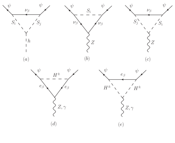
Figure 3: One-loop effective couplings between the fermion DM candidate and the SM neutral bosons.

$$\frac{d\sigma_{\psi T}}{dE_{R}} =F^{2}_{c}(E_{R})\left\{\frac{Z^{2}e^{2}}{4\pi}\left[\frac{1}{E_{R}}-\frac{1}{E^{max}_{R}(v^{2}_{rel})}\right]\left(C^{\gamma}_{M}\right)^{2}+\frac{Z^{2}e^{2}}{4\pi v^{2}_{rel}}\frac{1}{E_{R}}\left(C^{\gamma}_{E}\right)^{2}\right.$$

$$\left.+\frac{m_{T}}{2\pi v^{2}_{rel}}\left|Z\left(f^{p}_{S}+f^{p}_{V}-eC^{\gamma}_{R}-\frac{e}{2m_{\psi}}C^{\gamma}_{M}\right)+\left(A-Z\right)\left(f^{n}_{S}+f^{n}_{V}\right)\right|^{2}\right\}.$$ (16)

Here $v_{rel}$ is the relative velocity between $\psi$ and the nucleus, and $E_{R}$ denotes the recoil energy of the nucleus due to the interaction. The maximum value of $E_{R}$, $E^{max}_{R}$, is related with $v_{rel}$ through

$$E^{max}_{R}(v^{2}_{rel})=\frac{2m^{2}_{\psi}m_{T}v^{2}_{rel}}{(m_{\psi}+m_{T})^{2}}.$$ (17)

The effective couplings $C^{\gamma}_{M\left(E\right)}$ and $C^{\gamma}_{R}$ correspond to the Wilson coefficients describing the interaction with the photon field as a result of the magnetic (electric) dipole moment and the charge radius of the fermion DM. In this model these quantities are given by

$$C^{\gamma}_{M} =-\dfrac{e}{2(4\pi)^{2}m_{\psi}}|y_{1\beta}|^{2}\ g_{M1}\left(m_{\psi},m_{H^{\pm}},m_{e_{\beta}}\right),$$ (18)

$$C^{\gamma}_{E} =0,$$ (19)

$$C^{\gamma}_{R} =-\dfrac{e}{2(4\pi)^{2}m^{2}_{\psi}}|y_{1\beta}|^{2}\ g_{R1}\left(m_{\psi},m_{H^{\pm}},m_{e_{\beta}}\right),$$ (20)

where explicit expressions for the one-loop functions $g_{M1}$ and $g_{R1}$ are reported in Appendix A. The vanishing of $C^{\gamma}_{E}$ has its origin in the absence of a coupling between the right-handed electron and $\psi$ as can be seen from Eq. (14). The interaction with nucleons is described by the effective scalar and vector couplings $f^{(N)}_{S}$ and $f^{(N)}_{V}$ $\left(N=p,n\right)$, respectively. The scalar coupling is given in terms of the $\psi$-quark (-gluon) scalar couplings $C^{q(g)}_{S}$ and the matrix elements $f^{(N)}_{T_{q}}=\langle N|m_{q}\overline{q}q|N\rangle/m_{N}$. From Ref. SHIFMAN1978443 it reads

$$f^{(N)}_{S} =m_{N}\left[\sum_{q=u,d,s}C^{q}_{S}f^{(N)}_{T_{q}}-\frac{8}{9}C^{g}_{S}f^{(N)}_{T_{G}}\right],$$ (21)

where $m_{N}$ is the nucleon mass. On the other hand, the vector coupling can be expressed in terms of the $\psi$-quark vector couplings $C^{q}_{V}$ as

$$f^{(N)}_{V} =\begin{cases}2C^{u}_{V}+C^{d}_{V},\,\,\,\mathrm{for}\ N=p\,,\\ C^{u}_{V}+2C^{d}_{V},\,\,\,\mathrm{for}\ N=n\,.\end{cases}$$ (22)

In this model, the $\psi$ effective interactions with quarks and gluons can be cast as

$$C^{q}_{S} =-4C^{g}_{S}=-\frac{1}{\sqrt{2}m^{2}_{h}v_{\mathrm{SM}}}C_{\psi h},$$ (23)

$$C^{u}_{V} =-\frac{2}{v^{2}_{\mathrm{SM}}}\left(\frac{1}{2}-\frac{4}{3}\sin^{2}\theta_{W}\right)C_{\psi Z},$$ (24)

$$C^{d}_{V} =-\frac{2}{v^{2}_{\mathrm{SM}}}\left(-\frac{1}{2}+\frac{2}{3}\sin^{2}\theta_{W}\right)C_{\psi Z},$$ (25)

being $C_{\psi h(Z)}$ the effective scalar (vector) coupling between $\psi$ and the Higgs ($Z$) boson. These are given by

$$C_{\psi h} =\frac{\tilde{g}_{h1}(m_{\psi},m_{S_{i}},m_{S_{j}},m_{\nu_{\beta}})}{\sqrt{2}(4\pi)^{2}m_{\psi}}C_{\Phi i}\left(\lambda_{h\Phi}v_{\mathrm{SM}}C_{\Phi j}+\frac{\lambda^{\prime}v_{S}}{2}C_{Hj}\right)$$

$$\times\left(|y_{1\beta}|^{2}C_{Hi}C_{Hj}+|h_{\beta 1}|^{2}C_{\Phi i}C_{\Phi j}\right),$$ (26)

$$C_{\psi Z} =\frac{|y_{1\beta}|^{2}}{2(4\pi)^{2}}\left\{\left(\sin^{2}\theta_{W}-\frac{1}{2}\right)\left[g_{Z1}(m_{\psi},m_{H^{\pm}},m_{e_{\beta}},m_{e_{\beta}})+\tilde{g}_{Z1}(m_{\psi},m_{H^{\pm}},m_{H^{\pm}},m_{e_{\beta}})\right]\right.$$

$$\left.+\sin^{2}\theta_{W}\frac{m^{2}_{e_{\beta}}}{m^{2}_{\psi}}\ g_{Z2}(m_{\psi},m_{H^{\pm}},m_{e_{\beta}},m_{e_{\beta}})+\frac{C^{2}_{Hi}}{2}\left[g_{Z1}(m_{\psi},m_{S_{i}},m_{\nu_{\beta}},m_{\nu_{\beta}})\right.\right.$$

$$\left.+\ C^{2}_{Hj}\tilde{g}_{Z1}(m_{\psi},m_{S_{i}},m_{S_{j}},m_{\nu_{\beta}})\right]\bigg{\}}+\frac{|h_{\beta 1}|^{2}}{2(4\pi)^{2}}\frac{C_{Hi}C_{\Phi i}C_{Hj}C_{\Phi j}}{2}\tilde{g}_{Z1}(m_{\psi},m_{S_{i}},m_{S_{j}},m_{\nu_{\beta}}).$$ (27)

As indicated above, a sum over repeated indices is implied and the definitions of the one-loop functions $\tilde{g}_{h1}$, $g_{Z1}$, $\tilde{g}_{Z1}$ and $g_{Z2}$ are reported in Appendix A. By last, the recoil-energy dependent nuclear form factor $F^{2}_{c}(E_{R})$ in Eq. (16) reads Lewin:1995rx ; Helm:1956zz

$$F^{2}_{c}(E_{R})=\left[3\frac{j_{1}(qR)}{qR}\right]^{2}e^{-q^{2}s^{2}},$$ (28)

where $j_{1}$ is the spherical Bessel function of the first kind, $q=\sqrt{2m_{T}E_{R}}$ and $R=\sqrt{c^{2}+\frac{7}{3}\pi^{2}a^{2}-5s^{2}}$ with $c=(1.23A^{1/3}-0.6)$ fm, $a=0.52$ fm and $s=0.9$ fm.

In order to estimate the expected number of $\psi$-nuclei scattering events in a direct detection experiment like XENON1T Aprile:2017iyp , we calculate the differential event rate per unit of detector mass through Hisano:2018bpz

$$\frac{dR}{dE_{R}}=\frac{\rho_{DM}}{m_{T}m_{\psi}}\int_{v_{min}(E_{R})}^{\infty}d^{3}\textbf{v}_{rel}v_{rel}f_{\oplus}(\textbf{v}_{rel})\frac{d\sigma_{\psi T}}{dE_{R}}.$$ (29)

Here $\rho_{DM}\approx 0.3$ GeV/cm³ is the local DM density, $v_{min}(E_{R})$ is the minimum speed needed to yield a recoil with energy $E_{R}$, which can be determined from

$$v_{min}(E_{R})=\sqrt{\frac{(m_{\psi}+m_{T})^{2}E_{R}}{2m^{2}_{\psi}m_{T}}},$$ (30)

and $f_{\oplus}(\textbf{v}_{rel})$ stands for the DM velocity distribution measured with respect to the lab frame. With respect to the galactic frame, this distribution is assumed to follow a Maxwell-Boltzmann one, i.e.

$$f(\mathbf{v})=\begin{cases}\frac{1}{N}e^{-|\mathbf{v}|^{2}/v^{2}_{0}},\ \text{for}\ \ |\mathbf{v}|<v_{\mathrm{esc}},\\ 0,\ \ \text{for}\ \ |\mathbf{v}|>v_{\mathrm{esc}},\end{cases}$$ (31)

where the maximum speed is equal to the galaxy escape velocity, $v_{\mathrm{esc}}$, and

$$N=\pi^{3/2}v^{3}_{0}\left[\mathrm{erf}\left(\dfrac{v_{\mathrm{esc}}}{v_{0}}\right)-\dfrac{2v_{\mathrm{esc}}}{\sqrt{\pi}v_{0}}e^{-\left(\frac{v_{\mathrm{esc}}}{v_{0}}\right)^{2}}\right].$$ (32)

In this way, if $\textbf{v}_{E}$ is the velocity of the Earth with respect to the galactic frame, then

$$f_{\oplus}(\mathbf{v}_{rel})=f(\mathbf{v}_{rel}+\mathbf{v}_{E}).$$ (33)

For the numerical analysis we took the values used by the XENON1T collaboration Aprile:2018dbl , namely, $v_{0}=220$ km/s, $v_{\mathrm{esc}}=544$ km/s and $v_{E}=232$ km/s.

In the case of the direct detection experiment XENON1T, the number of expected events, $\mathcal{N}_{events}$, can be determined as Aprile:2011hx

$$\mathcal{N}_{events}=\omega_{exp}\int_{S_{min}}^{S_{max}}dS\sum_{n=1}^{\infty}\text{Gauss}(S|n,\sqrt{n}\sigma_{PMT})\int_{0}^{\infty}dE_{R}\epsilon(E_{R})\text{Poiss}(n|\nu(E_{R}))\frac{dR}{dE_{R}}.$$ (34)

Here $\omega_{exp}$ $=278.8$ days$\times$1.30 ton is the exposure, $S\in[3,70]$ is the number of photo-electrons (PE) resulting from the collision between the WIMP DM candidate and a Xe nucleus $\left(A=131\right.$, $Z=54$, $m_{T}=122.0$ GeV$\left.\right)$; $\sigma_{PMT}$ is the average single-PE resolution of the photo-multipliers, $\epsilon(E_{R})$ is the detection efficiency and $\nu(E_{R})$ is the expected number of PEs for a given recoil energy $E_{R}$. For the numerical estimate of $\mathcal{N}_{events}$ we took $\sigma_{PMT}=0.4$ Aprile:2015lha ; Barrow:2016doe , whereas $\epsilon(E_{R})$ was extracted from the black solid line in figure 1 of Ref. Aprile:2018dbl . $\nu(E_{R})$, for its part, was calculated as

$$\nu(E_{R})=E_{R}\ \mathcal{L}_{eff}\ \mathcal{L}_{y}\ S_{NR},$$ (35)

where the average light yield $\mathcal{L}y$ was fixed in 7.7 PE/keV Aprile:2015uzo and a value of 0.95 was assigned to the light yield suppression factor for nuclear recoils $S_{NR}$. The relative scintillation efficiency $\mathcal{L}_{eff}$ was extracted from figure 1 in Ref. Aprile:2011hi .

From the most recent data reported by XENON1T, and with the aid of a Test Statistic (TS), we can obtain an upper bound for $\mathcal{N}_{events}$. Closely following Ref. Cirelli:2013ufw , we take

$$\text{TS}(m_{\psi})=-2\ln\left[\frac{\mathcal{L}(\mathcal{N}_{events})}{\mathcal{L}_{BG}}\right],$$ (36)

with

$$\mathcal{L}(\mathcal{N}_{events})=\frac{(\mathcal{N}_{events}+\mathcal{N}_{BG})^{\mathcal{N}_{obs}}}{\mathcal{N}_{obs}!}e^{-(\mathcal{N}_{events}+\mathcal{N}_{BG})},$$ (37)

and $\mathcal{L}_{BG}\equiv\mathcal{L}(0)$. It follows that by demanding $\text{TS}(m_{\psi})>2.71$, limits for $\mathcal{N}_{events}$ are obtained at 90% CL. For $\mathcal{N}_{obs}=14$ (number of observed events) and $\mathcal{N}_{BG}=7.36(61)$ (number of background events) Aprile:2018dbl , the expected number of events must fulfill $\mathcal{N}_{events}\lesssim 19.5$ Hisano:2018bpz .

IV Numerical results

$1\,{\rm GeV}\leq m_{\psi_{1}}\leq 500\,{\rm GeV}$
$2\,m_{\psi_{1}}\leq m_{\psi_{2}}\leq 1\,{\rm TeV}$
${\rm max}\left(1.5\,m_{\psi_{1}},70\,{\rm GeV}\right)\leq m_{S_{1}}\leq 1\,{\rm TeV}$
$m_{S_{1}}\leq m_{S_{2}}\leq 2\,{\rm TeV}$
$-\pi/2\leq\varphi\leq\pi/2$
$10^{-5}\leq|h_{\beta j}|\leq\sqrt{4\pi}$
$10^{9}\,{\rm GeV}\leq v_{S}\leq 10^{13}\,{\rm GeV}$
$0<\theta_{a}\leq 2\pi$

Table 2: Random sampling for the relevant free parameters used in the numerical analysis.

In order to study the fermion DM phenomenology and take into account the constraints associated with charged LFV processes, we have implemented the model in SARAH Staub:2013tta ; Staub:2015kfa to calculate, via SPheno Porod:2003um ; Porod:2011nf and FlavorKit Porod:2014xia , the flavor observables. In addition, we have used micrOMEGAs Belanger:2013oya to calculate the $\psi$ relic abundance. We have performed a random scan over the relevant free parameters of the model as shown in Table 2 and assumed $\lambda_{2}=\lambda_{\Phi}=\lambda_{h\Phi}=\lambda_{S}=0.01$. Moreover, the mass of the exotic quark, $M_{D}$, has been set to $\sim 10$ TeV along with $f_{\beta}=0.1$ in order to avoid the LHC constraints (see below). Let us recall that the $y_{i\beta}$ Yukawa couplings are linked to neutrino masses and the PMNS mixing matrix elements through the $h_{\beta j}$ Yukawa couplings as shown in section II. The LEP II constraints Achard:2001qw ; Lundstrom:2008ai on the $H^{\pm}$ charged scalar are automatically satisfied by the scan conditions defined in Table 2 and we also ensure that the oblique parameters $S$, $T$ and $U$ remain at $3\sigma$ level Baak:2014ora . Concerning to the neutrino parameters, we consider both hierarchies for neutrino masses and use the best fit points values reported in Ref. deSalas:2017kay for the $\mathcal{CP}$ conserving case. Finally, regarding the charged LFV processes we consider the current experimental bounds and their future expectations as shown in table 3.

Observable		Present limit		Future sensitivity
$\mathcal{B}(\mu\to e\gamma)$		$5.3\times 10^{-13}$ Adam:2013mnn		$6.3\times 10^{-14}$ Baldini:2013ke ; MEGII:2018kmf
$\mathcal{B}(\tau\to e\gamma)$		$3.3\times 10^{-8}$ Aubert:2009ag ; Bona:2007qt ; Miyazaki:2012mx		$3\times 10^{-9}$ Aushev:2010bq
$\mathcal{B}(\tau\to\mu\gamma)$		$4.4\times 10^{-8}$ Aubert:2009ag ; Bona:2007qt ; Miyazaki:2012mx		$3\times 10^{-9}$ Aushev:2010bq
$\mathcal{B}(\mu\to eee)$		$1.0\times 10^{-12}$ Bellgardt:1987du		$10^{-16}$ Blondel:2013ia
$\mathcal{B}(\tau\to eee)$		$4.4\times 10^{-8}$ Hayasaka:2010np		$3\times 10^{-9}$ Aushev:2010bq
$\mathcal{B}(\tau\to\mu\mu\mu)$		$2.1\times 10^{-8}$ Hayasaka:2010np		$10^{-9}$ Aushev:2010bq
${\rm R_{\mu e}({\rm Ti})}$		$4.3\times 10^{-12}$ Dohmen:1993mp		$10^{-18}$ Abrams:2012er
${\rm R_{\mu e}({\rm Au})}$		$7.3\times 10^{-13}$ Bertl:2006up		$-$

Table 3: Current bounds and projected sensitivities for charged LFV observables.

We have calculated the fermion DM one-loop scattering cross section and estimated the expected number of events in direct detection experiments, $\mathcal{N}_{\text{events}}$, following the procedure described in Sec. III. The results are shown in Figs. 4 and 5. In Fig. 4, we present $\mathcal{N}_{\text{events}}$ as a function of the scalar mixing angle ($|\sin\varphi|$). All the points satisfy the current LFV constraints and the current limit imposed by the XENON1T collaboration. The prospect limits expected by XENONnT are indicated by the horizontal dashed line Aprile:2018dbl . Notice that a large fraction of the parameter space (red points) will be explored in the next years (those featuring a small mixing angle are beyond the projected sensitivity, although such a small mixing angle is favoured by the tiny neutrino masses). From Fig. 4 we also notice that for either $\varphi\rightarrow 0$ or $\varphi\rightarrow\pm\,\pi/2$, the number of events decreases rapidly, being steeper for $|\varphi|\to\pi/2$. This happens because when $\varphi\rightarrow 0$, the effective coupling between $\psi$ and the Higgs $\left(C_{\psi h}\right)$ becomes more suppressed than the case $|\varphi|\rightarrow\pi/2$ (see Eq. (26)). However, the coupling between $\psi$ and the Z boson ($C_{\psi Z}$) remains unaltered for both cases. Consequently, the expected number of events falls down more slowly for low small mixing angles. On the other hand, when the mixing is appreciable the contributions to $C_{\psi h}$ and $C_{\psi Z}$ coming from the neutral component of the scalar doublet $H_{2}$ become relevant, thus increasing the number of events in such a way it becomes maximum for $\varphi\sim\pi/4$.

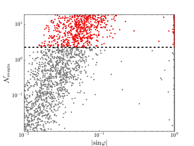
Figure 4: Expected number of events as a function of the scalar mixing angle. All the points satisfy the current limit imposed XENON1T and the dashed line denotes the projected sensitivity of XENONnT experiment Aprile:2018dbl .

In Fig. 5 we display the mass splitting $\Delta M\equiv m_{H^{\pm}}-m_{\psi}$ as a function of the scalar mixing angle. As in Fig. 4, the gray points are allowed by the current experimental searches, whereas the red ones represent the region that will be explored in the next years. Notice that in the case of maximal mixing $\left(|\varphi|\sim\pi/4\right)$, where the number of events reaches its maximum value, there are some points localized in the allowed region. For these points the mass splitting between the charged scalar and $\psi$ is small, $\Delta M\lesssim 50$ GeV, which means that the co-annihilation processes are relevant. Conversely, for either $\varphi\rightarrow 0$ or $\varphi\rightarrow\pm\,\pi/2$ where the number of events drops sharply, the mass splitting can take any value in the allowed range determined in the scan.

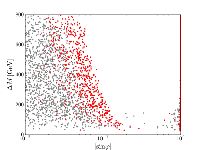
Figure 5: The mass splitting $\Delta M\equiv m_{H^{\pm}}-m_{\psi}$ as a function of the scalar mixing angle. All the points satisfy the current limit imposed XENON1T and the red ones are those that will be explored by XENONnT.

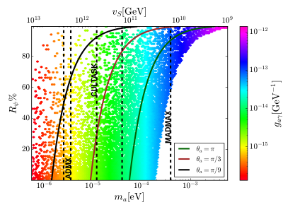
Figure 6: $\psi$ contribution to the total DM relic density as a function of the axion mass $m_{a}$ and the axion-photon coupling, $g_{a\gamma}\sim\frac{\alpha}{2\pi v_{S}}$, for different values of the initial misalignment angle $\theta_{a}$. The vertical dashed lines represent the regions that will be explored by the cavity haloscope experiments ADMX ADMX:2018gho ; Braine:2019fqb , CULTASK Semertzidis:2019gkj ; Chung:2018wms and MADMAX Caldwell:2016dcw ; MADMAX:2019pub ; Millar:2016cjp ; Horns:2012jf .

We now turn to discuss the axion phenomenology. The contribution of $\psi$ to the total DM relic density $R_{\psi}=\Omega_{\psi}/(\Omega_{\psi}+\Omega_{a})$ as a function of the axion mass is shown in Fig. 6. Each point reproduces the observed DM relic density $\Omega h^{2}=0.120\pm 0.001$ at $3\sigma$ Planck:2018vyg and satisfies the direct detection constraints on $\psi$ as well as the charged LFV bounds. The color code represents the corresponding axion-photon coupling, $g_{a\gamma}\sim\frac{\alpha}{2\pi v_{S}}$, which plays a main role in axion searches through helioscope and haloscope experiments Sikivie:2020zpn ; Graham:2015ouw ; Irastorza:2018dyq . For $v_{S}\lesssim 10^{10}$ GeV the main contribution to the DM relic abundance comes from the fermion DM candidate, with the corresponding axion mass window laying outside the experimental searches. However, for increasing values of $v_{S}$ the mixed fermion-axion DM scenario becomes more relevant and the axion can account for a fraction or the whole of the DM relic abundance. In this case, a large fraction of the axion mass window (with the axion-photon coupling taking values in the range $g_{a\gamma}\sim(5\times 10^{-16}-10^{-13})$ GeV^-1) can be explored by several haloscope experiments Graham:2015ouw ; Irastorza:2018dyq : ADMX for $m_{a}\sim(2.5-3.5)~{}\mu$eV, CULTASK for $m_{a}\sim(3.5-12)~{}\mu$eV and MADMAX for $m_{a}\sim(0.04-0.4)$ meV. Let us notice, however, that some regions are beyond the reach of the projected sensitivity of the experiments. Nonetheless, by enlarging the particle content or changing the PQ charge assignment on the current fields of the model, the chiral anomaly coefficient in the $g_{a\gamma}$ coupling can be modified in such a way that the entire region planned to search QCD axions in KSVZ and DFSZ models becomes experimentally accessible Graham:2015ouw ; Irastorza:2018dyq ; DiLuzio:2017pfr .

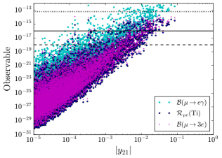
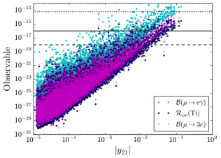
Figure 7: Branching ratios for charged LFV processes involving muons as a function of $|y_{21}|$ for the normal (left) and inverted (right) neutrino mass hierarchy.

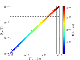
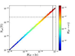
Figure 8: Correlation between the different LFV observables involving muons. The left and right panels correspond to a IH and NH, respectively. The solid and dashed lines represent the expected sensitivity for the future searches $\mathcal{B}(\mu\rightarrow 3e)$ and $\mathcal{R}_{\mu e}$, respectively.

Regarding the charged LFV processes, we focus in the observables involving muons in the initial state. In Fig. 7 are displayed the branching ratios $\mathcal{B}(\mu\rightarrow e\gamma)$ (cyan points), $\mathcal{B}(\mu\rightarrow 3e)$ (magenta points) and the rate for the $\mu\rightarrow e$ conversion in titanium $\mathcal{R}_{\mu e}$ (blue points) as a function of the Yukawa coupling $y_{21}$. The left (right) panel stands for the normal (inverted) neutrino mass hierarchy, with the dotted, solid and dashed horizontal lines representing the projected sensitivity of LFV experiments for $\mathcal{B}(\mu\rightarrow e\gamma)$, $\mathcal{B}(\mu\rightarrow 3e)$ and $\mathcal{R}_{\mu e}$, respectively. It follows that for both neutrino mass hierarchies the current bounds demand $|y_{21}|\lesssim 0.1$ whereas the future searches will explore values as low as 0.01, with the conversion in nuclei being the most relevant process (we have found similar results for the other Yukawa couplings $y_{i\beta}$). In addition to this, we notice that the observables associated with the lepton conversion in nuclei and the process with three electrons in the final state are strongly correlated. This is because the conversion process in nuclei does not involve box diagrams whereas the corresponding contribution in $\mu\rightarrow 3e$ becomes suppressed by a factor $|y_{i\beta}|^{4}$ and therefore the penguin diagrams give the dominant contribution for both charged LFV processes. This strong correlation, along with the correlation from $\mathcal{B}(\mu\rightarrow e\gamma)$, is shown in Fig. 8. On the other hand, we observed that the Yukawa couplings $h_{\beta i}$ can take values along the whole range considered in the scan. This result along with the ones for $y_{i\beta}$ discussed above translate to that the scalar coupling $|\lambda^{\prime}|$ lies below $10^{-7}$ in order to reproduce the observed neutrino mass scale (see Eq. (9)).

A final comment is in order concerning the exotic quark $D$. Since it couples to the SM sector through the Yukawa term, $\overline{q_{L}}H_{2}D_{R}$, it can decay into a $S_{1,2}$ scalar and a SM quark, thus avoiding potential issues that arise when an exotic quark is considered cosmologically stable Nardi:1990ku . Furthermore, such an exotic quark can be produced at colliders via quark and gluon fusion, leading to the specific signature of jets plus missing energy. From the analysis presented in Ref. Alves:2016bib , which deals with a scenario similar to the one studied here, the LHC searches for exotic quarks imply that $M_{D}\gtrsim$ 700 GeV, which is well below the value considered in our analysis.

V Conclusions

In the class of models known as scotogenic models the generation of radiative neutrino masses is associated with the existence of a discrete symmetry that forbids the tree-level contribution and stabilizes the DM particle. On these lines, the PQ symmetry can also be invoked to simultaneously provide a solution to the strong CP problem, radiatively induce neutrino masses and stabilize the particles lying in the dark sector. In this work we considered a multicomponent scotogenic model with Dirac neutrinos where the dark sector is composed by the QCD axion and a SM singlet fermion, the latter stabilized by the PQ symmetry. We computed the expected number of fermion-DM nuclei scatterings in XENON1T and identified regions of the parameter space compatible with observed DM abundance, direct searches of singlet fermion and axion DM, neutrino oscillation data and the upper bounds on charged LFV processes. Furthermore, we find that for some choices of parameters both the singlet fermion and the axion present detection rates are within the expected sensitivity of XENONnT and haloscope experiments such as ADMX, CULTASK, and MADMAX, respectively, and that the LFV processes involving muons in the initial state may be probed in upcoming rare leptonic decay experiments.

VI Acknowledgments

We are thankful to Diego Restrepo and Nicolás Bernal for enlightening discussions. This work has been supported by Sostenibilidad-UdeA and the UdeA/CODI Grants 2017-16286 and 2020-33177. Cristian D. R. Carvajal and Robinson Longas acknowledge the financial support given by COLCIENCIAS through the doctoral scholarship 727-2015 and 617-2013.

Appendix A One-loop functions for effective interactions of fermion DM

In this section we reproduce the expressions for the one-loop functions required to calculate the $C^{\gamma}_{M}$, $C^{\gamma}_{R}$, $C_{\psi h}$ and $C_{\psi Z}$ effective couplings Hisano:2018bpz . The functions associated with $C_{M}^{\gamma}$, $C_{R}^{\gamma}$ and $C_{\psi h}$ and are given by

$$g_{M1}(m_{\psi},M,m) =1-\frac{M^{2}-m^{2}}{2m^{2}_{\psi}}\mathrm{ln}\left(\frac{M^{2}}{m^{2}}\right)+\frac{\Delta+m^{2}_{\psi}\left(M^{2}-m^{2}_{\psi}+m^{2}\right)}{2m^{2}_{\psi}}L,$$ (38)

$$g_{R1}(m_{\psi},M,m) =\frac{1}{12}\left[\frac{8\left(M^{2}-m^{2}\right)+m^{2}_{\psi}}{m^{2}_{\psi}}\mathrm{ln}\left(\frac{M^{2}}{m^{2}}\right)-\frac{4}{\Delta}\left\{4\Delta+m^{2}_{\psi}\left(M^{2}+3m^{2}\right)-m^{4}_{\psi}\right\}\right.$$

$$\left.-\frac{L}{m^{2}_{\psi}\Delta}\left\{8\Delta^{2}+\left(9M^{2}-5m^{2}_{\psi}+7m^{2}\right)m^{2}_{\psi}\Delta-4m^{2}m^{4}_{\psi}\left(3M^{2}-m^{2}_{\psi}+m^{2}\right)\right\}\right],$$ (39)

whereas, the one associated with $C_{\psi h}$ reads

$$\tilde{g}_{h1}\left(m_{\psi},M_{i},M_{j},m\right) =\frac{1}{2}+\frac{M^{2}_{i}+M^{2}_{j}-2\left(m^{2}+m^{2}_{\psi}\right)}{4m^{2}_{\psi}}\mathrm{ln}\left(\frac{m^{2}}{M_{i}M_{j}}\right)$$

$$-\frac{M^{4}_{i}+M^{4}_{j}-2\left(M^{2}_{i}+M^{2}_{j}\right)\left(m^{2}+m^{2}_{\psi}\right)-2\left(m^{4}_{\psi}-m^{4}\right)}{4m^{2}_{\psi}\left(M^{2}_{i}-M^{2}_{j}\right)}\mathrm{ln}\left(\frac{M_{i}}{M_{j}}\right)$$

$$+\frac{(M^{2}_{i}-m^{2}-m^{2}_{\psi})\Delta_{i}L_{i}-(M^{2}_{j}-m^{2}-m^{2}_{\psi})\Delta_{j}L_{j}}{4m^{2}_{\psi}(M^{2}_{i}-M^{2}_{j})}.$$ (40)

The computation of $C_{\psi Z}$ involves the functions

$$g_{Z1}(m_{\psi},M,m_{i},m_{j}) =-\frac{1}{2}\Delta_{\epsilon,\mu}+\frac{1}{2}\mathrm{ln}\ M+\frac{m^{2}_{i}\ \mathrm{ln}\ m_{i}-m^{2}_{j}\ \mathrm{ln}\ m_{j}}{2\left(m^{2}_{i}-m^{2}_{j}\right)}+\frac{m^{2}_{i}+m^{2}_{j}-2M^{2}-m^{2}_{\psi}}{2m^{2}_{\psi}}$$

$$+\dfrac{\mathrm{ln}\left(\frac{M^{2}}{m_{i}m_{j}}\right)}{4m^{4}_{\psi}}\left[m^{4}_{i}+m^{4}_{j}-m^{2}_{i}m^{2}_{j}-3M^{2}\left(m^{2}_{i}+m^{2}_{j}-M^{2}\right)\right.$$

$$\left.-m^{2}_{\psi}\left(m^{2}_{i}+m^{2}_{j}+2M^{2}\right)\right]-\frac{\mathrm{ln}\left(\frac{m_{i}}{m_{j}}\right)}{4m^{4}_{\psi}\left(m^{2}_{i}-m^{2}_{j}\right)}\left\{2m^{6}_{\psi}-6m^{4}_{\psi}M^{2}+m^{2}_{\psi}\left[6M^{4}\right.\right.$$

$$\left.\left.-2M^{2}\left(m^{2}_{i}+m^{2}_{j}\right)-m^{4}_{i}-m^{4}_{j}\right]-2M^{6}+3M^{4}\left(m^{2}_{i}+m^{2}_{j}\right)-3M^{2}\left(m^{4}_{i}+m^{4}_{j}\right)\right.$$

$$\left.+m^{6}_{i}+m^{6}_{j}\right\}+\frac{1}{4m^{4}_{\psi}\left(m^{2}_{i}-m^{2}_{j}\right)}\left\{\left[\left(M^{2}-m^{2}_{i}\right)^{2}+\left(M^{2}-m^{2}_{\psi}\right)^{2}-M^{4}\right]\Delta_{i}L_{i}\right.$$

$$\left.-\left[\left(M^{2}-m^{2}_{j}\right)^{2}+\left(M^{2}-m^{2}_{\psi}\right)^{2}-M^{4}\right]\Delta_{j}L_{j}\right\},$$ (41)

$$g_{Z2}(m_{\psi},M,m_{i},m_{j}) =\frac{1}{2}\mathrm{ln}\left(\frac{M^{2}}{m_{i}m_{j}}\right)+\frac{\mathrm{ln}\left(\frac{m_{i}}{m_{j}}\right)}{2\left(m^{2}_{i}-m^{2}_{j}\right)}\left(2M^{2}-2m^{2}_{\psi}-m^{2}_{i}-m^{2}_{j}\right)$$

$$+\frac{\Delta_{i}L_{i}-\Delta_{j}L_{j}}{2\left(m^{2}_{i}-m^{2}_{j}\right)},$$ (42)

$$\tilde{g}_{Z1}(m_{\psi},M_{i},M_{j},m) =\frac{1}{2}\Delta_{\epsilon,\mu}-\frac{1}{2}\mathrm{ln}\ m-\frac{M^{2}_{i}\ \mathrm{ln}\ M_{i}-M^{2}_{j}\ \mathrm{ln}\ M_{j}}{2\left(M^{2}_{i}-M^{2}_{j}\right)}+\frac{M^{2}_{i}+M^{2}_{j}-2m^{2}+m^{2}_{\psi}}{2m^{2}_{\psi}}$$

$$+\frac{3m^{2}\left(m^{2}-M^{2}_{i}-M^{2}_{j}\right)-m^{2}_{\psi}\left(M^{2}_{i}+M^{2}_{j}\right)+M^{4}_{i}+M^{4}_{j}+M^{2}_{i}M^{2}_{j}}{4m^{4}_{\psi}}\mathrm{ln}\left(\frac{m^{2}}{M_{i}M_{j}}\right)$$

$$-\frac{\mathrm{ln}\left(\frac{M_{i}}{M_{j}}\right)}{4m^{4}_{\psi}\left(M^{2}_{i}-M^{2}_{j}\right)}\left[M^{6}_{i}+M^{6}_{j}-\left(3m^{2}+m^{2}_{\psi}\right)\left(M^{4}_{i}+M^{4}_{j}\right)+3m^{4}\left(M^{2}_{i}+M^{2}_{j}\right)\right.$$

$$\left.-2\left(m^{2}-m^{2}_{\psi}\right)^{2}\left(m^{2}+m^{2}_{\psi}\right)\right]+\frac{1}{4m^{4}_{\psi}\left(M^{2}_{i}-M^{2}_{j}\right)}\left\{\left[\left(M^{2}_{i}-m^{2}\right)^{2}-m^{4}_{\psi}\right]\Delta_{i}L_{i}\right.$$

$$\left.-\left[\left(M^{2}_{j}-m^{2}\right)^{2}-m^{4}_{\psi}\right]\Delta_{j}L_{j}\right\},$$ (43)

where

$$\Delta\left(m_{\psi},M,m\right) =m^{4}_{\psi}-2m^{2}_{\psi}\left(M^{2}+m^{2}\right)+\left(M^{2}-m^{2}\right)^{2}$$

$$=m^{4}-2m^{2}\left(M^{2}+m^{2}_{\psi}\right)+\left(M^{2}-m^{2}_{\psi}\right)^{2}$$

$$=M^{4}-2M^{2}\left(m^{2}_{\psi}+m^{2}\right)+\left(m^{2}_{\psi}-m^{2}\right)^{2},$$ (44)

and

$$L\left(m_{\psi},M,m\right)=\frac{1}{\sqrt{\Delta}}\mathrm{ln}\left(\frac{M^{2}+m^{2}-m^{2}_{\psi}+\sqrt{\Delta}}{M^{2}+m^{2}-m^{2}_{\psi}-\sqrt{\Delta}}\right).$$ (45)

Additionally, $\Delta_{i}$ and $L_{i}$ denote the quantities $\Delta(m_{\psi},M_{i},m)$ and $L(m_{\psi},M_{i},m)$, respectively, while $\Delta_{\epsilon,\mu}$ is a divergent constant term.

From these general expressions we deduce appropriated formulas for the limiting cases $m\to 0$, $M_{i}=M_{j}$ and $m_{i}=m_{j}$. In what follows, and when possible, the resulting expressions will be written in terms of the parameters $x\equiv\dfrac{m}{M}$, $y\equiv\dfrac{m_{\psi}}{M}$ and $\delta\equiv x^{4}-2x^{2}(1+y^{2})+(1-y^{2})^{2}$. Thus, for example,

$$g_{M1}(m_{\psi},M,m) =1+\frac{1-x^{2}}{y^{2}}\mathrm{ln}\ x+\frac{(1-x^{2})^{2}-(1+x^{2})y^{2}}{2y^{2}\sqrt{\delta}}\mathrm{ln}\left(\frac{1+x^{2}-y^{2}+\sqrt{\delta}}{1+x^{2}-y^{2}-\sqrt{\delta}}\right),$$ (46)

$$g_{R1}(m_{\psi},M,m) =-\frac{1}{6}\left[8\frac{1-x^{2}}{y^{2}}+1\right]\mathrm{ln}\ x-\frac{1}{3\delta}\left[4(1-x^{2})^{2}-(7+5x^{2})y^{2}+3y^{4}\right]$$

$$-\frac{1}{12y^{2}\delta^{3/2}}\mathrm{ln}\left(\frac{1+x^{2}-y^{2}+\sqrt{\delta}}{1+x^{2}-y^{2}-\sqrt{\delta}}\right)\left[8(1-x^{2})^{4}-(1-x^{2})^{2}(23+25x^{2})y^{2}\right.$$

$$\left.+(25-2x^{2}+25x^{4})y^{4}-(13+11x^{2})y^{6}+3y^{8}\right].$$ (47)

For the case $M_{i}\neq M_{j}$ and $m=0$ we obtain

$$\tilde{g}_{h1}(m_{\psi},M_{i},M_{j},0) =\frac{1}{2}+\frac{m^{2}_{\psi}}{M^{2}_{i}-M^{2}_{j}}\mathrm{ln}\left(\frac{M_{i}}{M_{j}}\right)$$

$$+\frac{(M^{2}_{i}-m^{2}_{\psi})^{2}\ \mathrm{ln}\left(\dfrac{M_{i}^{2}-m^{2}_{\psi}}{M^{2}_{i}}\right)-(M^{2}_{j}-m^{2}_{\psi})^{2}\ \mathrm{ln}\left(\dfrac{M_{j}^{2}-m^{2}_{\psi}}{M^{2}_{j}}\right)}{2m^{2}_{\psi}(M^{2}_{i}-M^{2}_{j})},$$ (48)

$$\tilde{g}_{Z1}(m_{\psi},M_{i},M_{j},0) =\frac{1}{2}\Delta_{\epsilon,\mu}+\frac{1}{2m^{4}_{\psi}(M^{2}_{i}-M^{2}_{j})}\left[(M^{4}_{i}-m^{4}_{\psi})(M^{2}_{i}-m^{2}_{\psi})\ \mathrm{ln}\left(\dfrac{M_{i}^{2}-m^{2}_{\psi}}{M^{2}_{i}}\right)\right.$$

$$\left.-(M^{4}_{j}-m^{4}_{\psi})(M^{2}_{j}-m^{2}_{\psi})\ \mathrm{ln}\left(\dfrac{M_{j}^{2}-m^{2}_{\psi}}{M^{2}_{j}}\right)\right]+\frac{M^{2}_{i}+M^{2}_{j}+m^{2}_{\psi}}{2m^{2}_{\psi}},$$ (49)

whereas for $M_{i}=M_{j}\equiv M$ and $m\neq 0$

$$\tilde{g}_{h1}(m_{\psi},M,M,m) =1+\frac{1-x^{2}-y^{2}}{y^{2}}\mathrm{ln}\ x+\frac{x^{4}-2x^{2}+(1-y^{2})^{2}}{2y^{2}\sqrt{\delta}}\mathrm{ln}\left(\frac{1+x^{2}-y^{2}+\sqrt{\delta}}{1+x^{2}-y^{2}-\sqrt{\delta}}\right),$$ (50)

$$\tilde{g}_{Z1}(m_{\psi},M,M,m) =\frac{1}{2}\Delta_{\epsilon,\mu}-\frac{1}{2}\mathrm{ln}(mM)+\frac{1}{4}+\frac{6-6x^{2}-y^{2}}{4y^{2}}+\frac{3-2y^{2}-3x^{2}(2-x^{2})}{2y^{4}}\mathrm{ln}\ x$$

$$+\frac{1}{4y^{4}\sqrt{\delta}}\mathrm{ln}\left(\frac{1+x^{2}-y^{2}+\sqrt{\delta}}{1+x^{2}-y^{2}-\sqrt{\delta}}\right)\left[3(1-x^{2})^{3}+(3x^{4}+2x^{2}-5)y^{2}\right.$$

$$\left.+(1-x^{2})y^{4}+y^{6}\right],$$ (51)

The case $M_{i}=M_{j}\equiv M$ and $m=0$ leads to

$$\tilde{g}_{h1}(m_{\psi},M,M,0) =1+\frac{1-y^{2}}{y^{2}}\mathrm{ln}\left(1-y^{2}\right)\ ,$$ (52)

$$\tilde{g}_{Z1}(m_{\psi},M,M,0) =\frac{1}{2}\Delta_{\epsilon,\mu}-\mathrm{ln}M+\frac{1}{4}-\frac{y^{2}-6}{4y^{2}}+\frac{3-5y^{2}+y^{4}+y^{6}}{2y^{4}(1-y^{2})}\mathrm{ln}(1-y^{2})\ ,$$ (53)

and the case $m_{i}=m_{j}\equiv m\neq 0$ involves the limiting functions

$$g_{Z1}(m_{\psi},M,m,m) =-\frac{1}{2}\Delta_{\epsilon,\mu}+\frac{1}{2}\mathrm{ln}(mM)-\frac{1}{4}-\frac{x^{4}+3(1-2x^{2})-2y^{2}(1+x^{2})}{2y^{4}}\mathrm{ln}\ x$$

$$-\frac{3(1-x^{2})^{3}-5(1-x^{4})y^{2}+(1-3x^{2})y^{4}+y^{6}}{4y^{4}\sqrt{\delta}}\mathrm{ln}\left(\frac{1+x^{2}-y^{2}+\sqrt{\delta}}{1+x^{2}-y^{2}-\sqrt{\delta}}\right)$$

$$+\frac{6x^{2}+y^{2}-6}{4y^{2}},$$ (54)

$$g_{Z2}(m_{\psi},M,m,m) =-\mathrm{ln}\ x-\frac{1-x^{2}+y^{2}}{2\sqrt{\delta}}\mathrm{ln}\left(\frac{1+x^{2}-y^{2}+\sqrt{\delta}}{1+x^{2}-y^{2}-\sqrt{\delta}}\right).$$ (55)

Finally, the limiting functions appearing in the case $m_{i}=m_{j}\equiv m=0$ fulfill

$$g_{Z1}(m_{\psi},M,0,0) =-\tilde{g}_{Z1}(m_{\psi},M,M,0).$$ (56)

Notice that, from Eqs. (51) and (54)

$$g_{Z1}(m_{\psi},M,m,m)+\tilde{g}_{Z1}(m_{\psi},M,M,m) =\frac{(x^{2}+y^{2})}{x^{-2}y^{4}}\mathrm{ln}\ x$$

$$+\frac{(1-x^{2}+y^{2})}{2x^{-2}y^{2}\sqrt{\delta}}\mathrm{ln}\left(\frac{1+x^{2}-y^{2}+\sqrt{\delta}}{1+x^{2}-y^{2}-\sqrt{\delta}}\right).$$ (57)

References

- (1) R. D. Peccei and Helen R. Quinn, “CP Conservation in the Presence of Instantons,” Phys. Rev. Lett. 38, 1440–1443 (1977), [,328(1977)]
- (2) Steven Weinberg, “A New Light Boson?.” Phys. Rev. Lett. 40, 223–226 (1978)
- (3) Frank Wilczek, “Problem of Strong p and t Invariance in the Presence of Instantons,” Phys. Rev. Lett. 40, 279–282 (1978)
- (4) Pierre Sikivie, “Axion Cosmology,” Lect. Notes Phys. 741, 19–50 (2008), arXiv:astro-ph/0610440
- (5) John Preskill, Mark B. Wise, and Frank Wilczek, “Cosmology of the Invisible Axion,” Phys. Lett. B120, 127–132 (1983), [,URL(1982)]
- (6) L. F. Abbott and P. Sikivie, “A Cosmological Bound on the Invisible Axion,” Phys. Lett. B120, 133–136 (1983), [,URL(1982)]
- (7) Michael Dine and Willy Fischler, “The Not So Harmless Axion,” Phys. Lett. B120, 137–141 (1983), [,URL(1982)]
- (8) Rabindra N. Mohapatra and Goran Senjanovic, “The Superlight Axion and Neutrino Masses,” Z. Phys. C17, 53–56 (1983)
- (9) Q. Shafi and F. W. Stecker, “Implications of a Class of Grand Unified Theories for Large Scale Structure in the Universe,” Phys. Rev. Lett. 53, 1292 (1984)
- (10) P. Langacker, R. D. Peccei, and T. Yanagida, “Invisible Axions and Light Neutrinos: Are They Connected?.” Mod. Phys. Lett. A1, 541 (1986)
- (11) Michael Shin, “Light Neutrino Masses and Strong CP Problem,” Phys. Rev. Lett. 59, 2515 (1987), [Erratum: Phys. Rev. Lett.60,383(1988)]
- (12) X. G. He and R. R. Volkas, “Models Featuring Spontaneous CP Violation: An Invisible Axion and Light Neutrino Masses,” Phys. Lett. B208, 261 (1988), [Erratum: Phys. Lett.B218,508(1989)]
- (13) Z. G. Berezhiani and M. Yu. Khlopov, “Cosmology of Spontaneously Broken Gauge Family Symmetry,” Z. Phys. C49, 73–78 (1991)
- (14) S. Bertolini and A. Santamaria, “The Strong CP problem and the solar neutrino puzzle: Are they related?.” Nucl. Phys. B357, 222–240 (1991)
- (15) Ernest Ma, “Making neutrinos massive with an axion in supersymmetry,” Phys. Lett. B514, 330–334 (2001), arXiv:hep-ph/0102008 [hep-ph]
- (16) Geraldine Servant, “Baryogenesis from Strong Violation and the QCD Axion,” Phys. Rev. Lett. 113, 171803 (2014), arXiv:1407.0030 [hep-ph]
- (17) Seyda Ipek and Tim M. P. Tait, “Early Cosmological Period of QCD Confinement,” Phys. Rev. Lett. 122, 112001 (2019), arXiv:1811.00559 [hep-ph]
- (18) Djuna Croon, Jessica N. Howard, Seyda Ipek, and Timothy M. P. Tait, “QCD baryogenesis,” Phys. Rev. D 101, 055042 (2020), arXiv:1911.01432 [hep-ph]
- (19) Raymond T. Co and Keisuke Harigaya, “Axiogenesis,” Phys. Rev. Lett. 124, 111602 (2020), arXiv:1910.02080 [hep-ph]
- (20) Andrei D. Linde, “Axions in inflationary cosmology,” Phys. Lett. B 259, 38–47 (1991)
- (21) Sarah Folkerts, Cristiano Germani, and Javier Redondo, “Axion Dark Matter and Planck favor non-minimal couplings to gravity,” Phys. Lett. B 728, 532–536 (2014), arXiv:1304.7270 [hep-ph]
- (22) Malcolm Fairbairn, Robert Hogan, and David J. E. Marsh, “Unifying inflation and dark matter with the Peccei-Quinn field: observable axions and observable tensors,” Phys. Rev. D 91, 023509 (2015), arXiv:1410.1752 [hep-ph]
- (23) Guillermo Ballesteros, Javier Redondo, Andreas Ringwald, and Carlos Tamarit, “Unifying inflation with the axion, dark matter, baryogenesis and the seesaw mechanism,” Phys. Rev. Lett. 118, 071802 (2017), arXiv:1608.05414 [hep-ph]
- (24) Cristian D. R. Carvajal and Óscar Zapata, “One-loop Dirac neutrino mass and mixed axion-WIMP dark matter,” Phys. Rev. D 99, 075009 (2019), arXiv:1812.06364 [hep-ph]
- (25) Chian-Shu Chen and Lu-Hsing Tsai, “Peccei-Quinn symmetry as the origin of Dirac Neutrino Masses,” Phys. Rev. D88, 055015 (2013), arXiv:1210.6264 [hep-ph]
- (26) Basudeb Dasgupta, Ernest Ma, and Koji Tsumura, “Weakly interacting massive particle dark matter and radiative neutrino mass from Peccei-Quinn symmetry,” Phys. Rev. D89, 041702 (2014), arXiv:1308.4138 [hep-ph]
- (27) Stefano Bertolini, Luca Di Luzio, Helena Kolešová, and Michal Malinský, “Massive neutrinos and invisible axion minimally connected,” Phys. Rev. D91, 055014 (2015), arXiv:1412.7105 [hep-ph]
- (28) Pei-Hong Gu, “Peccei-Quinn symmetry for Dirac seesaw and leptogenesis,” JCAP 1607, 004 (2016), arXiv:1603.05070 [hep-ph]
- (29) Ernest Ma, Diego Restrepo, and Óscar Zapata, “Anomalous leptonic U(1) symmetry: Syndetic origin of the QCD axion, weak-scale dark matter, and radiative neutrino mass,” Mod. Phys. Lett. A33, 1850024 (2018), arXiv:1706.08240 [hep-ph]
- (30) Ernest Ma, Takahiro Ohata, and Koji Tsumura, “Majoron as the QCD axion in a radiative seesaw model,” Phys. Rev. D96, 075039 (2017), arXiv:1708.03076 [hep-ph]
- (31) Daijiro Suematsu, “Dark matter stability and one-loop neutrino mass generation based on Peccei–Quinn symmetry,” Eur. Phys. J. C78, 33 (2018), arXiv:1709.02886 [hep-ph]
- (32) Daijiro Suematsu, “Possible roles of Peccei-Quinn symmetry in an effective low energy model,” Phys. Rev. D96, 115004 (2017), arXiv:1709.07607 [hep-ph]
- (33) Mario Reig, José W. F. Valle, and Frank Wilczek, “SO(3) family symmetry and axions,” Phys. Rev. D98, 095008 (2018), arXiv:1805.08048 [hep-ph]
- (34) Mario Reig and Rahul Srivastava, “Spontaneous proton decay and the origin of Peccei–Quinn symmetry,” Phys. Lett. B 790, 134–139 (2019), arXiv:1809.02093 [hep-ph]
- (35) Eduardo Peinado, Mario Reig, Rahul Srivastava, and Jose W. F. Valle, “Dirac neutrinos from Peccei–Quinn symmetry: A fresh look at the axion,” Mod. Phys. Lett. A 35, 2050176 (2020), arXiv:1910.02961 [hep-ph]
- (36) Seungwon Baek, “Dirac neutrino from the breaking of Peccei-Quinn symmetry,” Phys. Lett. B 805, 135415 (2020), arXiv:1911.04210 [hep-ph]
- (37) Leon M. G. de la Vega, Newton Nath, and Eduardo Peinado, “Dirac neutrinos from Peccei-Quinn symmetry: two examples,” Nucl. Phys. B 957, 115099 (2020), arXiv:2001.01846 [hep-ph]
- (38) Alex G. Dias, Julio Leite, José W. F. Valle, and Carlos A. Vaquera-Araujo, “Reloading the axion in a 3-3-1 setup,” Phys. Lett. B 810, 135829 (2020), arXiv:2008.10650 [hep-ph]
- (39) Seungwon Baek, “A connection between flavour anomaly, neutrino mass, and axion,” JHEP 10, 111 (2020), arXiv:2006.02050 [hep-ph]
- (40) Ernest Ma and Oleg Popov, “Pathways to Naturally Small Dirac Neutrino Masses,” Phys. Lett. B764, 142–144 (2017), arXiv:1609.02538 [hep-ph]
- (41) Chang-Yuan Yao and Gui-Jun Ding, “Systematic analysis of Dirac neutrino masses from a dimension five operator,” Phys. Rev. D97, 095042 (2018), arXiv:1802.05231 [hep-ph]
- (42) Howard Baer, Andre Lessa, Shibi Rajagopalan, and Warintorn Sreethawong, “Mixed axion/neutralino cold dark matter in supersymmetric models,” JCAP 1106, 031 (2011), arXiv:1103.5413 [hep-ph]
- (43) Kyu Jung Bae, Howard Baer, and Eung Jin Chun, “Mixed axion/neutralino dark matter in the SUSY DFSZ axion model,” JCAP 1312, 028 (2013), arXiv:1309.5365 [hep-ph]
- (44) Alexandre Alves, Daniel A. Camargo, Alex G. Dias, Robinson Longas, Celso C. Nishi, and Farinaldo S. Queiroz, “Collider and Dark Matter Searches in the Inert Doublet Model from Peccei-Quinn Symmetry,” JHEP 10, 015 (2016), arXiv:1606.07086 [hep-ph]
- (45) Suman Chatterjee, Anirban Das, Tousik Samui, and Manibrata Sen, “Mixed WIMP-axion dark matter,” Phys. Rev. D 100, 115050 (2019), arXiv:1810.09471 [hep-ph]
- (46) Jihn E. Kim, “Weak Interaction Singlet and Strong CP Invariance,” Phys. Rev. Lett. 43, 103 (1979)
- (47) Mikhail A. Shifman, A. I. Vainshtein, and Valentin I. Zakharov, “Can Confinement Ensure Natural CP Invariance of Strong Interactions?.” Nucl. Phys. B166, 493–506 (1980)
- (48) Yasaman Farzan and Ernest Ma, “Dirac neutrino mass generation from dark matter,” Phys. Rev. D86, 033007 (2012), arXiv:1204.4890 [hep-ph]
- (49) Weijian Wang and Zhi-Long Han, “Naturally Small Dirac Neutrino Mass with Intermediate Multiplet Fields,” JHEP(2016), doi:“bibinfo–doi˝–10.1007/JHEP04(2017)166˝, [JHEP04,166(2017)], arXiv:1611.03240 [hep-ph]
- (50) Debasish Borah and Arnab Dasgupta, “Common Origin of Neutrino Mass, Dark Matter and Dirac Leptogenesis,” JCAP 1612, 034 (2016), arXiv:1608.03872 [hep-ph]
- (51) Weijian Wang, Ronghui Wang, Zhi-Long Han, and Jin-Zhong Han, “The Scotogenic Models for Dirac Neutrino Masses,” Eur. Phys. J. C77, 889 (2017), arXiv:1705.00414 [hep-ph]
- (52) Chang-Yuan Yao and Gui-Jun Ding, “Systematic Study of One-Loop Dirac Neutrino Masses and Viable Dark Matter Candidates,” Phys. Rev. D96, 095004 (2017), arXiv:1707.09786 [hep-ph]
- (53) Ernest Ma and Utpal Sarkar, “Radiative Left-Right Dirac Neutrino Mass,” Phys. Lett. B776, 54–57 (2018), arXiv:1707.07698 [hep-ph]
- (54) M. Reig, D. Restrepo, J. W. F. Valle, and O. Zapata, “Bound-state dark matter and Dirac neutrino masses,” Phys. Rev. D97, 115032 (2018), arXiv:1803.08528 [hep-ph]
- (55) Julian Calle, Diego Restrepo, Carlos E. Yaguna, and Óscar Zapata, “Minimal radiative Dirac neutrino mass models,” Phys. Rev. D 99, 075008 (2019), arXiv:1812.05523 [hep-ph]
- (56) Julian Calle, Diego Restrepo, and Óscar Zapata, “Dirac neutrino mass generation from a Majorana messenger,” Phys. Rev. D 101, 035004 (2020), arXiv:1909.09574 [hep-ph]
- (57) Nicolás Bernal, Julián Calle, and Diego Restrepo, “Anomaly-free Abelian gauge symmetries with Dirac scotogenic models,” Phys. Rev. D 103, 095032 (2021), arXiv:2102.06211 [hep-ph]
- (58) P. A. Zyla et al. (Particle Data Group), “Review of Particle Physics,” PTEP 2020, 083C01 (2020)
- (59) Ernesto Arganda and Maria J. Herrero, “Testing supersymmetry with lepton flavor violating tau and mu decays,” Phys. Rev. D 73, 055003 (2006), arXiv:hep-ph/0510405
- (60) Florian Staub, “SARAH 4 : A tool for (not only SUSY) model builders,” Comput. Phys. Commun. 185, 1773–1790 (2014), arXiv:1309.7223 [hep-ph]
- (61) Florian Staub, “Exploring new models in all detail with SARAH,” Adv. High Energy Phys. 2015, 840780 (2015), arXiv:1503.04200 [hep-ph]
- (62) Werner Porod, “SPheno, a program for calculating supersymmetric spectra, SUSY particle decays and SUSY particle production at e+ e- colliders,” Comput. Phys. Commun. 153, 275–315 (2003), arXiv:hep-ph/0301101 [hep-ph]
- (63) W. Porod and F. Staub, “SPheno 3.1: Extensions including flavour, CP-phases and models beyond the MSSM,” Comput. Phys. Commun. 183, 2458–2469 (2012), arXiv:1104.1573 [hep-ph]
- (64) Werner Porod, Florian Staub, and Avelino Vicente, “A Flavor Kit for BSM models,” Eur. Phys. J. C74, 2992 (2014), arXiv:1405.1434 [hep-ph]
- (65) Giovanni Grilli di Cortona, Edward Hardy, Javier Pardo Vega, and Giovanni Villadoro, “The QCD axion, precisely,” JHEP 01, 034 (2016), arXiv:1511.02867 [hep-ph]
- (66) Luca Di Luzio, Maurizio Giannotti, Enrico Nardi, and Luca Visinelli, “The landscape of QCD axion models,” Phys. Rept. 870, 1–117 (2020), arXiv:2003.01100 [hep-ph]
- (67) Paola Arias, Davide Cadamuro, Mark Goodsell, Joerg Jaeckel, Javier Redondo, and Andreas Ringwald, “WISPy Cold Dark Matter,” JCAP 1206, 013 (2012), arXiv:1201.5902 [hep-ph]
- (68) Richard Lynn Davis, “Goldstone Bosons in String Models of Galaxy Formation,” Phys. Rev. D 32, 3172 (1985)
- (69) Diego Harari and P. Sikivie, “On the Evolution of Global Strings in the Early Universe,” Phys. Lett. B 195, 361–365 (1987)
- (70) R. A. Battye and E. P. S. Shellard, “Axion string constraints,” Phys. Rev. Lett. 73, 2954–2957 (1994), [Erratum: Phys.Rev.Lett. 76, 2203–2204 (1996)], arXiv:astro-ph/9403018
- (71) Takashi Hiramatsu, Masahiro Kawasaki, Ken’ichi Saikawa, and Toyokazu Sekiguchi, “Production of dark matter axions from collapse of string-wall systems,” Phys. Rev. D85, 105020 (2012), [Erratum: Phys. Rev.D86,089902(2012)], arXiv:1202.5851 [hep-ph]
- (72) Kyu Jung Bae, Ji-Haeng Huh, and Jihn E. Kim, “Update of axion CDM energy,” JCAP 09, 005 (2008), arXiv:0806.0497 [hep-ph]
- (73) G. Belanger, F. Boudjema, A. Pukhov, and A. Semenov, “micrOMEGAs3: A program for calculating dark matter observables,” Comput. Phys. Commun. 185, 960–985 (2014), arXiv:1305.0237 [hep-ph]
- (74) Junji Hisano, Ryo Nagai, and Natsumi Nagata, “Singlet Dirac Fermion Dark Matter with Mediators at Loop,” JHEP 12, 059 (2018), arXiv:1808.06301 [hep-ph]
- (75) John Ellis, Natsumi Nagata, and Keith A. Olive, “Uncertainties in WIMP Dark Matter Scattering Revisited,” Eur. Phys. J. C 78, 569 (2018), arXiv:1805.09795 [hep-ph]
- (76) M.A. Shifman, A.I. Vainshtein, and V.I. Zakharov, “Remarks on higgs-boson interactions with nucleons,” Physics Letters B 78, 443–446 (1978), ISSN 0370-2693, https://www.sciencedirect.com/science/article/pii/0370269378904811
- (77) J. D. Lewin and P. F. Smith, “Review of mathematics, numerical factors, and corrections for dark matter experiments based on elastic nuclear recoil,” Astropart. Phys. 6, 87–112 (1996)
- (78) Richard H. Helm, “Inelastic and Elastic Scattering of 187-Mev Electrons from Selected Even-Even Nuclei,” Phys. Rev. 104, 1466–1475 (1956)
- (79) E. Aprile et al. (XENON), “First Dark Matter Search Results from the XENON1T Experiment,” Phys. Rev. Lett. 119, 181301 (2017), arXiv:1705.06655 [astro-ph.CO]
- (80) E. Aprile et al. (XENON), “Dark Matter Search Results from a One Ton-Year Exposure of XENON1T,” Phys. Rev. Lett. 121, 111302 (2018), arXiv:1805.12562 [astro-ph.CO]
- (81) E. Aprile et al. (XENON100), “Likelihood Approach to the First Dark Matter Results from XENON100,” Phys. Rev. D 84, 052003 (2011), arXiv:1103.0303 [hep-ex]
- (82) E. Aprile et al. (XENON), “Lowering the radioactivity of the photomultiplier tubes for the XENON1T dark matter experiment,” Eur. Phys. J. C 75, 546 (2015), arXiv:1503.07698 [astro-ph.IM]
- (83) P. Barrow et al., “Qualification Tests of the R11410-21 Photomultiplier Tubes for the XENON1T Detector,” JINST 12, P01024 (2017), arXiv:1609.01654 [astro-ph.IM]
- (84) E. Aprile et al. (XENON), “Physics reach of the XENON1T dark matter experiment,” JCAP 04, 027 (2016), arXiv:1512.07501 [physics.ins-det]
- (85) E. Aprile et al. (XENON100), “Dark Matter Results from 100 Live Days of XENON100 Data,” Phys. Rev. Lett. 107, 131302 (2011), arXiv:1104.2549 [astro-ph.CO]
- (86) Marco Cirelli, Eugenio Del Nobile, and Paolo Panci, “Tools for model-independent bounds in direct dark matter searches,” JCAP 10, 019 (2013), arXiv:1307.5955 [hep-ph]
- (87) P. Achard et al. (L3), “Search for heavy neutral and charged leptons in annihilation at LEP,” Phys. Lett. B 517, 75–85 (2001), arXiv:hep-ex/0107015
- (88) Erik Lundstrom, Michael Gustafsson, and Joakim Edsjo, “The Inert Doublet Model and LEP II Limits,” Phys. Rev. D 79, 035013 (2009), arXiv:0810.3924 [hep-ph]
- (89) M. Baak, J. Cúth, J. Haller, A. Hoecker, R. Kogler, K. Mönig, M. Schott, and J. Stelzer (Gfitter Group), “The global electroweak fit at NNLO and prospects for the LHC and ILC,” Eur. Phys. J. C 74, 3046 (2014), arXiv:1407.3792 [hep-ph]
- (90) P. F. de Salas, D. V. Forero, C. A. Ternes, M. Tortola, and J. W. F. Valle, “Status of neutrino oscillations 2018: 3 hint for normal mass ordering and improved CP sensitivity,” Phys. Lett. B782, 633–640 (2018), arXiv:1708.01186 [hep-ph]
- (91) J. Adam et al. (MEG), “New constraint on the existence of the decay,” Phys. Rev. Lett. 110, 201801 (2013), arXiv:1303.0754 [hep-ex]
- (92) A.M. Baldini, F. Cei, C. Cerri, S. Dussoni, L. Galli, et al., “MEG Upgrade Proposal,” (2013), arXiv:1301.7225 [physics.ins-det]
- (93) A. M. Baldini et al. (MEG II), “The design of the MEG II experiment,” Eur. Phys. J. C 78, 380 (2018), arXiv:1801.04688 [physics.ins-det]
- (94) Bernard Aubert et al. (BaBar Collaboration), “Searches for Lepton Flavor Violation in the Decays and ,” Phys.Rev.Lett. 104, 021802 (2010), arXiv:0908.2381 [hep-ex]
- (95) M. Bona et al. (SuperB), “SuperB: A High-Luminosity Asymmetric e+ e- Super Flavor Factory. Conceptual Design Report,” (2007), arXiv:0709.0451 [hep-ex]
- (96) Y. Miyazaki et al. (Belle), “Search for Lepton-Flavor-Violating and Lepton-Number-Violating Decay Modes,” Phys. Lett. B719, 346–353 (2013), arXiv:1206.5595 [hep-ex]
- (97) T. Aushev et al., “Physics at Super B Factory,” (2010), arXiv:1002.5012 [hep-ex]
- (98) U. Bellgardt et al. (SINDRUM Collaboration), “Search for the Decay ,” Nucl.Phys. B299, 1 (1988)
- (99) A. Blondel, A. Bravar, M. Pohl, S. Bachmann, N. Berger, et al., “Research Proposal for an Experiment to Search for the Decay ,” (2013), arXiv:1301.6113 [physics.ins-det]
- (100) K. Hayasaka et al., “Search for Lepton Flavor Violating Tau Decays into Three Leptons with 719 Million Produced Tau+Tau- Pairs,” Phys. Lett. B687, 139–143 (2010), arXiv:1001.3221 [hep-ex]
- (101) C. Dohmen et al. (SINDRUM II), “Test of lepton flavor conservation in mu —¿ e conversion on titanium,” Phys. Lett. B317, 631–636 (1993)
- (102) R.J. Abrams et al. (Mu2e), “Mu2e Conceptual Design Report,” (2012), arXiv:1211.7019 [physics.ins-det]
- (103) Wilhelm H. Bertl et al. (SINDRUM II), “A Search for muon to electron conversion in muonic gold,” Eur. Phys. J. C47, 337–346 (2006)
- (104) N. Du et al. (ADMX), “A Search for Invisible Axion Dark Matter with the Axion Dark Matter Experiment,” Phys. Rev. Lett. 120, 151301 (2018), arXiv:1804.05750 [hep-ex]
- (105) T. Braine et al. (ADMX), “Extended Search for the Invisible Axion with the Axion Dark Matter Experiment,” Phys. Rev. Lett. 124, 101303 (2020), arXiv:1910.08638 [hep-ex]
- (106) Yannis K. Semertzidis et al., “Axion Dark Matter Research with IBS/CAPP,” (10 2019), arXiv:1910.11591 [physics.ins-det]
- (107) Woohyun Chung, “CULTASK, Axion Experiment at CAPP in Korea,” in 13th Patras Workshop on Axions, WIMPs and WISPs (2018) pp. 97–101
- (108) Allen Caldwell, Gia Dvali, Béla Majorovits, Alexander Millar, Georg Raffelt, Javier Redondo, Olaf Reimann, Frank Simon, and Frank Steffen (MADMAX Working Group), “Dielectric Haloscopes: A New Way to Detect Axion Dark Matter,” Phys. Rev. Lett. 118, 091801 (2017), arXiv:1611.05865 [physics.ins-det]
- (109) P. Brun et al. (MADMAX), “A new experimental approach to probe QCD axion dark matter in the mass range above 40 eV,” Eur. Phys. J. C 79, 186 (2019), arXiv:1901.07401 [physics.ins-det]
- (110) Alexander J. Millar, Georg G. Raffelt, Javier Redondo, and Frank D. Steffen, “Dielectric Haloscopes to Search for Axion Dark Matter: Theoretical Foundations,” JCAP 01, 061 (2017), arXiv:1612.07057 [hep-ph]
- (111) Dieter Horns, Joerg Jaeckel, Axel Lindner, Andrei Lobanov, Javier Redondo, and Andreas Ringwald, “Searching for WISPy Cold Dark Matter with a Dish Antenna,” JCAP 04, 016 (2013), arXiv:1212.2970 [hep-ph]
- (112) N. Aghanim et al. (Planck), “Planck 2018 results. VI. Cosmological parameters,” Astron. Astrophys. 641, A6 (2020), [Erratum: Astron.Astrophys. 652, C4 (2021)], arXiv:1807.06209 [astro-ph.CO]
- (113) Pierre Sikivie, “Invisible Axion Search Methods,” Rev. Mod. Phys. 93, 015004 (2021), arXiv:2003.02206 [hep-ph]
- (114) Peter W. Graham, Igor G. Irastorza, Steven K. Lamoreaux, Axel Lindner, and Karl A. van Bibber, “Experimental Searches for the Axion and Axion-Like Particles,” Ann. Rev. Nucl. Part. Sci. 65, 485–514 (2015), arXiv:1602.00039 [hep-ex]
- (115) Igor G. Irastorza and Javier Redondo, “New experimental approaches in the search for axion-like particles,” Prog. Part. Nucl. Phys. 102, 89–159 (2018), arXiv:1801.08127 [hep-ph]
- (116) Luca Di Luzio, Federico Mescia, and Enrico Nardi, “Window for preferred axion models,” Phys. Rev. D96, 075003 (2017), arXiv:1705.05370 [hep-ph]
- (117) Enrico Nardi and Esteban Roulet, “Are exotic stable quarks cosmologically allowed?.” Phys. Lett. B245, 105–110 (1990)