Online Facility Location with Linear Delay

Abstract

In the problem of online facility location with delay, a sequence of $n$ clients appear in the metric space, and they need to be eventually connected to some open facility. The clients do not have to be connected immediately, but such a choice comes with a certain penalty: each client incurs a waiting cost (equal to the difference between its arrival and its connection time). At any point in time, an algorithm may decide to open a facility and connect any subset of clients to it. That is, an algorithm needs to balance three types of costs: cost of opening facilities, costs of connecting clients, and the waiting costs of clients. We study a natural variant of this problem, where clients may be connected also to an already open facility, but such action incurs an extra cost: an algorithm pays for waiting of the facility (a cost incurred separately for each such “late” connection). This is reminiscent of online matching with delays, where both sides of the connection incur a waiting cost. We call this variant two-sided delay to differentiate it from the previously studied one-sided delay, where clients may connect to a facility only at its opening time.

We present an $O(1)$-competitive deterministic algorithm for the two-sided delay variant. Our approach is an extension of the approach used by Jain, Mahdian and Saberi [STOC 2002] for analyzing the performance of offline algorithms for facility location. To this end, we substantially simplify the part of the original argument in which a bound on the sequence of factor-revealing LPs is derived. We then show how to transform our $O(1)$-competitive algorithm for the two-sided delay variant to $O(\log n/\log\log n)$-competitive deterministic algorithm for one-sided delays. This improves the known $O(\log n)$ bound by Azar and Touitou [FOCS 2020]. We note that all previous online algorithms for problems with delays in general metrics have at least logarithmic ratios.

1 Introduction

The facility location problem [1] is one of the best-known examples of network design problems, extensively studied both in operations research and in computer science. The problem is defined in a metric space $\mathcal{X}$. An algorithm is given a set of $n$ clients and its goal is to open a set of facilities (chosen points of $\mathcal{X}$) minimizing the total cost, defined as the sum of costs of opening facilities plus the costs of connecting clients. Our focus is on the non-uniform case, where the opening cost of a facility may depend on its position in $\mathcal{X}$. The connection cost of a given client is simply its distance to the nearest open facility. This simple statement hides a surprisingly rich combinatorial structure and gave rise to series of algorithms and extensions. In particular, the problem is NP-complete and APX-hard [31] and its approximation ratio has been studied in a long sequence of improvements [41, 36, 34, 33, 25, 23, 39, 21], with the current record of 1.488 proved by Li [37].

In the online scenario, the set of clients is not known up-front, but it is revealed to an (online) algorithm one element at a time. Once a client becomes known, an algorithm has to make an irrevocable and immediate decision whether to open additional facilities and to which facility the current client should be connected. As in the offline scenario, the algorithm is compared to the best offline solution, and in online scenarios, we use the name competitive ratio instead of approximation ratio. This scenario has been fully resolved: tight asymptotic lower and upper bounds of $\Theta(\log n/\log\log n)$ are known both for randomized and deterministic algorithms [40, 2, 29, 30].

In the last few years, many online problems have been considered in scenarios with delays. In the case of online facility location, first studied by Azar and Touitou [9], the clients arrive in time, and while each of them has to be connected eventually, such action does not have to be executed immediately. This additional degree of freedom comes, however, with a price: each waiting client incurs an extra cost that (in the basic setting studied in this paper) is equal to its total waiting time (time between its arrival and its connection). We note that in terms of achievable competitive ratios, the classic models and models with delays are rarely comparable as the possibility of delaying actions is allowed also in the benchmark offline solution.

Facility location with one-sided delay

This variant has been introduced and studied in [9, 10]. There each facility is ephemeral: it is opened only momentarily at time $t$ chosen by an algorithm, and all connections to this facility must be made at time $t$. The algorithm can open another facility at the same location at a different time $t^{\prime}$, but the opening cost must be paid again. The waiting costs of clients are as described above.

The best known algorithm for this problem variant is $O(\log n)$-competitive [10]. (Interestingly, it is not known whether this particular variant admits constant-factor approximation in the offline setting when all client arrivals are known up-front.)

Facility location with two-sided delay

We propose the following slight deviation from the one-sided variant described above: once a facility becomes open at time $t$, it remains open forever and can be connected to in the future. However, any client that connects to such facility at time $t^{\prime}>t$ needs to pay an additional waiting cost of $t^{\prime}-t$. We call this amount facility-side waiting cost, which needs to be paid on top of the “standard” (client-side) waiting cost. We emphasize that such connections, dubbed late connections, can be made both by clients that arrived before facility opening and also after this time. Similarly to the one-sided delay model, we allow opening of multiple facilities in the same location at different points in time.

The two-sided model can be seen as an approximation of the early-late adopter behavior in crowdfunding models. In crowdfunding platforms for technology products [42] such as Kickstarter, any specific project is started by gathering initial contributions by enthusiasts up to a certain threshold, which should (in an ideal case) imply opening of a production line for the specified technology product. Contributors in this pre-production phase are called early adopters.

As we move forward in time, while the production may already begin, it may still be possible for so-called late adopters to join the crowdfunding project on the Kickstarter website and receive the final product. As early adoption is more beneficial for the producer of the technology product, late adoption is sometimes penalized with an increased cost of the same product compared to the early adoption.

In the framework of crowdfunding models, we can see online facility location with two-sided delay as facility location in an early-late adopter setting, where a technology product can be manufactured at multiple factories and late adopters may join into the crowdfunding scheme and thus contribute towards offsetting the cost of the production while it is in progress. However, the clients who join late need to deal with the missed-opportunity cost (the client-side cost) as well as the late adopter increase in price (the facility-side waiting cost).

1.1 Our Results and Techniques

Our first positive contribution is showing that facility location with two-sided delay admits a constant-competitive online algorithm, which is an important open problem for the one-sided case. Namely, we show:

Theorem 1.1.

There exists an $3.869$-competitive deterministic algorithm for the online facility location problem with two-sided delay, where all waiting costs are equal to the waiting times.

We analyze a natural greedy algorithm, which grows budgets with increasing waiting delays and opens facilities for subsets of clients once sums of these budgets reach certain thresholds. To analyze this algorithm, we use dual fitting methods. Our analysis is a substantial extension of the approach used by Jain et al. [34, 33] for analyzing the performance of offline algorithms for (non-delayed) facility location.

The central part of the analysis is a linear program (LP), parameterized by an integer $k$, whose objective value is an upper bound on the competitive ratio of our algorithm provided the number of clients in the input is at most $k$. As the objective function of this LP grows with $k$, simply solving the LP would yield the correct upper bound only for instances of limited size. As a replacement for the technical original argument in [33] we propose a much more intuitive one that is based on an upper bound to this sequence by the value of a finite linear program.

We would like to stress that we see our novel approach to the competitive analysis of facility location dual-fitting LP as an important contribution of this paper to the area of facility location with delays. Our approach has a significant computer-assisted component (Section 4) and it can thus be quickly deployed to give provable estimates on the potential competitive ratio or an approximation ratio of factor-revealing linear programs in other settings. Our code for the algorithmic part is publicly available [13].

Our second result is showing that $O(1)$-competitive algorithm for the two-sided variant yields an improved guarantee also for the one-sided variant.

Theorem 1.2.

There exists an $O(\log n/\log\log n)$-competitive deterministic algorithm for the online facility location problem with one-sided delay, where all waiting costs are equal to the waiting times.

We prove this result via a reduction that can be applied to any algorithm solving the two-sided variant provided it satisfies a certain technical condition that we call sensibility. Informally speaking this property means that the waiting costs associated with late connections are not very large; we defer the precise definition to Section 3.

Theorem 1.2 improves the known $O(\log n)$-bound by Azar and Touitou [10]. While the improvement is small, we note that all previous online algorithms for problems with delays have at least logarithmic ratios (in the number of used points of the metric space), so ours is the first to break this natural barrier.

1.2 Related work

Recently many online graph problems have been considered in a variant that allows requests to be delayed. Apart from the facility location problem studied in this paper, examples include the Steiner tree problem [9, 10], multi-level aggregation [15, 24, 19, 9, 11, 12], Steiner forest/network [10], directed Steiner tree [10], multi-cut [10], online matching [27, 3, 4, 17, 16, 38, 28, 6, 8], set cover [22, 5] and $k$-server (known in this setting as online service with delay) [7, 18, 9].

That said, the concept of delaying requests itself is not new. Famous studied problems include the TCP acknowledgement problem [26, 35] and joint replenishment problem [20, 14] (that are equivalent to the recently studied multi-level aggregation problem on one-level or two-level trees).

General waiting costs

The waiting costs considered in this paper are equal to waiting times. Another studied case are deadlines, where waiting costs are zero till a request-specific time (the deadline) and infinite afterwards. For some problems, easier algorithms or better bounds are known when the waiting costs are in the deadline form (see, e.g., [14, 19]).

Many of the results listed above can be extended to waiting costs being arbitrary non-decreasing left-continuous functions of waiting times. These extensions are straightforward if an algorithm is defined by simple thresholds on (sums of) waiting costs; when these thresholds are reached, they trigger an appropriate action of the algorithm. For instance, algorithms for the TCP acknowledgement problem were constructed for linear waiting costs, but they can be trivially extended to general costs.

There are however a few cases where general waiting costs are more problematic. Most notably, the online matching problem was studied for linear waiting costs [27, 3, 4, 17, 16, 28, 6], then shown to be more difficult (in terms of achievable competitive ratios) for convex waiting costs [38], and only recently competitive algorithms were shown for concave waiting costs [8].

The algorithms presented in this paper also fall into the latter category: our LP-based analysis heavily depends on the linearity of the waiting functions, and thus our algorithms cannot be easily extended to general waiting costs. (We note that the $O(\log n)$-competitive algorithm by Azar and Touitou [10] can handle arbitrary waiting costs.)

1.3 Remark about Facility-Side Waiting Costs

Recall that in the two-sided variant that we study in our paper, we assume that each late connection incurs an additional waiting cost at the facility side (equal to the time that passes between facility opening and client connection). Below, we argue that setting this cost to zero would cause the optimal competitive ratio to be $\Theta(\log n/\log\log n)$. This shows that for the $O(1)$-competitive result of Theorem 1.1, some assumptions about waiting cost functions are necessary.

In the two-sided variant of the facility location problem with delays, setting facility-side waiting costs to zero causes the optimal competitive ratio (both deterministic and randomized) to become asymptotically equal to $\Theta(\log n/\log\log n)$.

Proof 1.3.

Assume no penalty for facility-side waiting. For any input instance, without an increase of the cost, Opt may open all its facilities at time $0$ and connect all clients immediately when they arrive. Thus, the optimal solution incurs no waiting cost at all.

As the waiting cost can be avoided also for an online algorithm (by serving all clients immediately upon their arrival), the desired competitive ratio can be attained by running an $O(\log n/\log\log n)$-competitive algorithm (deterministic or randomized) for the online facility location problem (without delays) [40, 30],

For showing a lower bound, we may simply use an adversarial strategy for the online facility location problem (without delays) [30]; however, now the next request is presented only after an algorithm serves the previous one. This way, waiting becomes useless for an online algorithm, and the lower bound of $\Omega(\log n/\log\log n)$ [30] applies also for the waiting model.

1.4 Preliminaries

We use the following notions throughout the paper.

The pair $(\mathcal{X},\mathrm{dist})$ denotes the underlying metric space with its distance function, and $\mathcal{Y}\subseteq\mathcal{X}$ denotes the positions of potential facilities. The function $\mathrm{open}:\mathcal{Y}\to\mathbb{R}_{\geqslant 0}\cup\{\infty\}$ defines the cost of opening a facility at a specific location.

The clients are numbered from $1$ to $n$ and arrive in time; each is associated with a point in $\mathcal{X}$. Their total number is not known up-front to an online algorithm. For a client $j$, we use $x_{j}$ to denote its position and $t_{j}$ to denote the time of its arrival. We say that a client is active from the time of its arrival until it gets connected to a facility by an online algorithm, and it is inactive after the connection.

At any time, an algorithm may open a facility at any point $y\in\mathcal{Y}$, paying opening cost $\mathrm{open}(y)$. An active client $j$ may be connected by an algorithm at time $t^{c}_{j}\geqslant t_{j}$ to a facility that was open at time $\tau$, such that

• $\tau=t^{c}_{j}$, for the one-sided delay variant;

• $\tau\leqslant t^{c}_{j}$, for the two-sided delay variant.

Such a connection incurs a connection cost $\mathrm{dist}(x_{j},y)$ and two types of waiting costs: a client-side waiting cost $t^{c}_{j}-t_{j}$ and a facility-side waiting cost $t^{c}_{j}-\tau$. Note that the latter waiting cost is always zero for the one-sided delay variant.

The goal of an algorithm is to minimize the total cost, defined as the sum of opening costs, connection costs, and waiting costs.

2 Algorithm for the Two-Sided Variant

We will now describe the algorithm for the online facility location with two-sided linear waiting cost. Our algorithm is parameterized with a constant $\gamma>1$ that will be fixed later. We say that an active client $j$ at time $t\geqslant t_{j}$, after experiencing waiting cost of $t-t_{j}$, has a connectivity budget

$$\alpha_{j}(t)=\gamma\cdot(t-t_{j}).$$

In the analysis, we use $\alpha_{j}$ to denote the connectivity budget of client $j$ at time $t^{c}_{j}$, when it becomes connected to a facility.

At any time $t$, for each potential facility location $y\in\mathcal{Y}$, an active client $j$ has an offer of a contribution towards the opening of a facility at $y$ equal to $\beta_{j}^{t}(y)=\max\{0,\alpha_{j}(t)-\mathrm{dist}(x_{j},y)\}$. When client $j$ becomes connected (and inactive), it no longer offers any contribution.

The algorithm follows the natural continuous flow of time of the online sequence and reacts to the events occurring throughout its runtime.

Algorithm 1.

At any time $t$, do the following.

If a new client $j$ arrives at point $x_{j}$ (client $j$ becomes active): From this time onward start growing its connectivity budget.

If for any location $y\in\mathcal{Y}$, the sum of offered contributions $\beta_{j}^{t}(y)$ towards this location from all the currently active clients reaches $\mathrm{open}(y)$ (the facility opening cost at $y$): Let $A^{t}(y)$ be the set of active clients $j$ for which $\alpha_{j}(t)\geqslant\mathrm{dist}(x_{j},y)$, i.e., those that can afford the distance. Open a facility at $y$, and connect every client $j\in A^{t}(y)$ to it.

If for a facility that has already been open at time $\tau\leqslant t$ at location $y$, and for an active client $j$, it holds that $t-\tau=\alpha_{j}(t)-\mathrm{dist}(x_{j},y)$: Connect client $j$ to this facility. We call this action late connection. In Case 1 and Case 1, all clients that get connected become inactive.

2.1 Basic observations

One may observe that Algorithm 1 is a generalization of (the simpler version of) the algorithm by Jain et al. [34]. Furthermore, if it is run on an instance where all clients appear at the same time, it produces the same solution (the same facility locations and the same connections) as the original offline approximation algorithm.

It is convenient to think that the connectivity budget of a client is first spent on connection cost, and the remaining part either contributes to the opening of a new facility or pays for the facility-side waiting cost of an already open facility.

The total cost of the solution produced by Algorithm 1 is $(1+1/\gamma)\cdot\sum_{j}\alpha_{j}$.

Proof 2.1.

The sum of opening costs, connection costs and facility-side waiting costs in the produced solution equals the sum of final connectivity budgets $\sum_{j}\alpha_{j}$. The total client-side waiting cost is $(1/\gamma)\cdot\sum_{j}\alpha_{j}$.

To estimate the competitive ratio of the algorithm, it thus suffices to compare the cost of the optimal solution to $(1+1/\gamma)\cdot\sum_{j}\alpha_{j}$, which we do in Section 3.

2.2 Sensibility

Our later construction for the one-sided waiting variant requires that the used online algorithm for the two-sided variant has the following property, which bounds the number of clients that connect late to an already open facility.

Definition 2.2 (sensibility).

Fix any $\lambda>1$ and $\xi>1$. An algorithm solving the two-sided variant is called $(\lambda,\xi)$-sensible if it satisfies the following property for any facility $f$ opened at time $\tau$ and location $y$: for any $w>0$, the number of clients connected to $f$ within the interval $\interval[openleft]{\tau+w}{\tau+\lambda\cdot w}$ is at most $\xi\cdot\mathrm{open}(y)/w$.

We show that for some constants $\lambda$ and $\xi$, our algorithm is $(\lambda,\xi)$-sensible: if clients connecting late to an open facility incurred large (facility-side) waiting costs, then our algorithm would rather create a new copy of this facility, and connect these clients to the copy.

Lemma 2.3.

Fix a parameter $\gamma>1$ of Algorithm 1. For any $\lambda\in(1,1+1/(\gamma-1))$, Algorithm 1 is $(\lambda,(\gamma-(\gamma-1)\cdot\lambda)^{-1})$-sensible.

Proof 2.4.

Fix a facility $f$ opened at time $\tau$ at location $y$. Let $C_{w}$ be the set of clients that are connected late to $f$ within interval $\interval[openleft]{\tau+w}{\tau+\lambda\cdot w}$. Take any client $j\in C_{w}$ and let $t^{c}_{j}=\tau+h$ be its connection time. We define the residual budget of client $j$ at time $t$ as $r_{j}(t)=\alpha_{j}(t)-\mathrm{dist}(x_{j},y)$.

We now estimate the residual budget of client $j$ at time $\tau+w$. Let $\tau+g$ be the time when its residual budget becomes zero, i.e., $r_{j}(\tau+g)=0$. Its residual budget at time $\tau+h$ is then $r_{j}(\tau+h)=\alpha_{j}(\tau+h)-\alpha_{j}(\tau+g)=\gamma\cdot(h-g)$. On the other hand, $r_{j}(\tau+h)=(\tau+h)-\tau=h$, as $j$ forms a late connection to $f$ at time $\tau+h$. Hence, $\gamma\cdot g=(\gamma-1)\cdot h\leqslant(\gamma-1)\cdot\lambda\cdot w$, which implies $r_{j}(\tau+w)=\gamma\cdot(w-g)\geqslant(\gamma-(\gamma-1)\cdot\lambda)\cdot w$. (Note that for our choice of $\lambda$, this amount is positive.)

By the definition of Algorithm 1, the residual budgets are spent either on opening new facilities or on facility-side waiting of an already opened facility. Hence, at time $\tau+w$, the sum of residual budgets of all clients from $C_{w}$ cannot be larger than $\mathrm{open}(y)$, as in such case Algorithm 1 would open another copy of the facility at $y$. This argument implies that $|C_{w}|\cdot(\gamma-(\gamma-1)\cdot\lambda)\cdot w\leqslant\mathrm{open}(y)$, which concludes the proof.

For example, by Lemma 2.3, Algorithm 1 with $\gamma=2$ is $(3/2,2)$-sensible.

3 Competitive Analysis via Factor Revealing LP

Fix an optimal offline solution. We will heavily use the structure of this solution being a collection of stars, each of them composed of a single open facility and a set of clients connected in the optimal solution to this facility. Just as in the analysis of the JMS algorithm [34, 33], we will focus on a single star $S$ of Opt, and compare $\sum_{j\in S}\alpha_{j}$ to the cost of this star.

Let $\tau$ be the time of opening the facility $f$ in the considered star $S$ of the optimal solution. Note that our online algorithm could connect clients $j\in S$ to facilities opened by the online algorithm both before and after $\tau$. For a client $j\in S$ that arrived at time $t_{j}$ and got connected by the algorithm at time $t_{j}^{c}$, we set $a_{j}=t_{j}-\tau$ and $s_{j}=t_{j}^{c}-\tau$ to denote the arrival time and the service time of $j$ (time when $j$ is connected to a facility by the algorithm) relative to $\tau$. Note that our algorithm grows $\alpha_{j}$ until it reaches value $\gamma\cdot(s_{j}-a_{j})$. Variable $d_{j}$ will denote the distance between the locations of the client $j$ and the facility $f$. Let $\mathrm{open}(f)$ denote the cost of opening the facility $f$.

Consider the following factor revealing LP:

Linear Program 1.

$$z_{k}{(\gamma)}=\max\frac{(1+\gamma)\cdot\sum_{i=0}^{k-1}(s_{i}-a_{i})}{\mathrm{open}(f)+\sum_{i=0}^{k-1}(d_{i}+|a_{i}|)}$$ (1a)

$$s_{i}\leqslant s_{i+1} \forall_{0\leqslant i<k-1}$$ (1b)

$$(\gamma-1)\cdot s_{i}-\gamma\cdot a_{i}\leqslant d_{i}+d_{j}+(\gamma-1)\cdot s_{j}-\gamma\cdot a_{j} \forall_{0\leqslant j<i<k}$$ (1c)

$$\sum_{i=\ell}^{k-1}\max{\{\gamma\cdot(s_{\ell}-a_{i})-d_{i},0\}}\leqslant\mathrm{open}(f) \forall_{\ell<k}$$ (1d)

$$d_{i}\geqslant 0,s_{i}\geqslant a_{i} \forall_{0\leqslant i<k}$$ (1e)

Lemma 3.1.

$z_{k}(\gamma)$ is an upper bound on the competitive ratio of the algorithm for a fixed value of parameter $\gamma$ on a star of Opt with $k$ clients.

Proof 3.2.

It suffices to argue that the constraints (1b-1e) are satisfied for any values $d_{i},a_{i},s_{i}$ representing the situation of clients from a single star of Opt in an actual run of the online algorithm.

We consider the set of clients in the order of them being connected by the online algorithm. If two clients are connected at the same time, we first take the one that arrived first. Constraints (1b) are trivially satisfied by this ordering.

Constraints (1d) reflect the situation just before time $t_{\ell}^{c}$ when client $\ell$ gets connected by Algorithm 1. The left-hand side is a sum of the contributions of still active clients towards opening a facility in the very same spot as Opt has a facility for this star. Obviously, these contributions cannot exceed the cost of opening a facility.

Finally, to argue for Constraints (1c) being satisfied we consider two cases. If $s_{i}=s_{j}$, then $a_{j}\leqslant a_{i}$, and the constraint is trivially satisfied. Otherwise, $s_{i}>s_{j}$. Consider the moment just before client $i$ gets connected. Client $i$ cannot have a budget that would be more than sufficient to connect to the facility where client $j$ is connected. The connectivity budget of $i$ is then $\gamma\cdot(s_{i}-a_{i})$ and the distance to the facility serving $j$ plus waiting at this facility for $i$ can be upper bounded by $d_{i}+d_{j}+(s_{i}-s_{j})+\gamma\cdot(s_{j}-a_{j})$, see Figure 1.

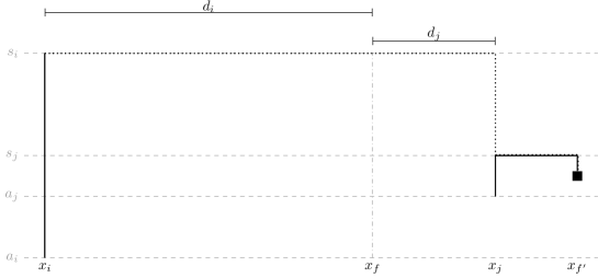
Figure 1: Illustration for Constraint (1c) (the triangle inequality). Before time $s_{i}$, the budget of client $i$ must not be sufficient to connect $i$ to the facility $f^{\prime}$ currently serving $j$—otherwise the algorithm would have already connected it. The cost of such a connection can be bounded by a sum of $d_{i}+d_{j}$ (upper bounds $\mathrm{dist}(x_{i},x_{j})$), $s_{i}-s_{j}$ (the waiting cost on the facility side since $s_{j}$), and $\gamma\cdot(s_{j}-a_{j})$ (upper-bounds $\mathrm{dist}(x_{j},y_{f^{\prime}})$ and the remainder of waiting of $f^{\prime}$).

3.1 Bounding the LP value

Here we will show an alternative (an in our opinion conceptually much simpler than the original one from Sec 5.2 of [33]) method to upper-bound a sequence of factor-revealing linear programs.

Our task now is to bound the value of $z_{k}(\gamma)$ for every $k$. It is insufficient to compute $z_{k}(\gamma)$ for some fixed $k$ as it is monotonically increasing with $k$ (a fact which we prove in a slightly weaker form). In this section, we will however show that it converges to a constant as $k$ goes to infinity.

Proposition 3.3.

For any $\gamma>0$ and $k,m\in\mathbb{N}_{+}$, it holds that $z_{k}(\gamma)\leqslant z_{k\cdot m}(\gamma)$.

Proof 3.4.

Let $\langle d,a,s\rangle\in\mathbb{R}^{k}\times\mathbb{R}^{k}\times\mathbb{R}^{k}$ be a solution to LP1 optimizing $z_{k}(\gamma)$. We will construct a solution $\langle d^{\prime},a^{\prime},s^{\prime}\rangle\in\mathbb{R}^{k\cdot m}\times\mathbb{R}^{k\cdot m}\times\mathbb{R}^{k\cdot m}$ of the same value.

For $i\in[k]$ and $r\in[m]$, let $d^{\prime}_{m\cdot i+r}=d_{i}/m$, $a^{\prime}_{m\cdot i+r}=a_{i}/m$, and $s^{\prime}_{m\cdot i+r}=s_{i}/m$. The inequalities (1b), (1c), and (1e) are satisfied by the new solution, since the same numbers appear in these inequalities in the solution $\langle d,a,s\rangle$. To show feasibility of $\langle d^{\prime},a^{\prime},s^{\prime}\rangle$ we need to argue that (1d) is satisfied for $\ell$ not divisible by $m$:

$$\sum_{i=\ell}^{m\cdot k-1} \max{\{\gamma\cdot(s^{\prime}_{\ell}-a^{\prime}_{i})-d^{\prime}_{i},0\}}$$

$$\leqslant\sum_{i=m\cdot\lfloor\ell/m\rfloor}^{m\cdot k-1}\max{\{\gamma\cdot(s^{\prime}_{\ell}-a^{\prime}_{i})-d^{\prime}_{i},0\}}$$ (more summands)

$$=\sum_{i=m\cdot\lfloor\ell/m\rfloor}^{m\cdot k-1}\max{\{\gamma\cdot(s^{\prime}_{m\cdot\lfloor\ell/m\rfloor}-a^{\prime}_{i})-d^{\prime}_{i},0\}} s^{\prime}_{\ell}=s^{\prime}_{m\cdot\lfloor\frac{\ell}{m}\rfloor}$$ (since )

$$=\sum_{i=\lfloor\ell/m\rfloor}^{k-1}\max{\{\gamma\cdot(s_{\lfloor\ell/m\rfloor}-a_{i})-d_{i},0\}} \langle d^{\prime},a^{\prime},s^{\prime}\rangle$$ (by definition of )

$$\leqslant\mathrm{open}(f).$$

To determine how $z(\gamma)$ converges, we will define another LP, whose optimal value will always upper-bound LP1.

Linear Program 2.

This program with optimal value equal $y_{k}(\gamma)$ is defined to be the same as LP1 except for the following inequality swapped for (1d):

$$\sum_{i=\ell\mathbf{+1}}^{k-1}\max{\{\gamma\cdot(s_{\ell}-a_{i})-d_{i},0\}}\leqslant\mathrm{open}(f) \forall_{l<k}.$$ (2d)

Proposition 3.5.

For any $\gamma>0$ and $k,m\in\mathbb{N}_{+}$ it holds that $y_{k}(\gamma)\geqslant y_{k\cdot m}(\gamma)$.

Proof 3.6.

Let $\langle d,a,s\rangle\in\mathbb{R}^{k\cdot m}\times\mathbb{R}^{k\cdot m}\times\mathbb{R}^{k\cdot m}$ be the solution to LP2 maximizing $y_{k\cdot m}(\gamma)$. We define a solution $\langle d^{\prime},a^{\prime},s^{\prime}\rangle\in\mathbb{R}^{k}\times\mathbb{R}^{k}\times\mathbb{R}^{k}$ of the same value as:

$$d^{\prime}_{i}=\sum_{r=0}^{m-1}d_{m\cdot i+r}, a^{\prime}_{i}=\sum_{r=0}^{m-1}a_{m\cdot i+r}, s^{\prime}_{i}=\sum_{r=0}^{m-1}s_{m\cdot i+r}, \forall_{0\leqslant i<k}.$$

Again, we only need to focus on the inequality (2d):

$$\sum_{i=\ell+1}^{k-1} \max\left\{\gamma\cdot(s^{\prime}_{\ell}-a^{\prime}_{i})-d^{\prime}_{i},0\right\}$$

$$=\sum_{i=\ell+1}^{k-1}\max\left\{\sum_{r=0}^{m-1}\gamma\cdot(s_{m\cdot\ell+r}-a_{m\cdot i+r})-d_{m\cdot i+r},0\right\} \langle d^{\prime},a^{\prime},s^{\prime}\rangle$$ (def. of )

$$\leqslant\sum_{i=\ell+1}^{k-1}\max\left\{\sum_{r=0}^{m-1}\gamma\cdot(s_{m\cdot(\ell+1)-1}-a_{m\cdot i+r})-d_{m\cdot i+r},0\right\} s_{i}$$ (monotonicity of )

$$\leqslant\sum_{i=\ell+1}^{k-1}\sum_{r=0}^{m-1}\max\left\{\gamma\cdot(s_{m\cdot(\ell+1)-1}-a_{m\cdot i+r})-d_{m\cdot i+r},0\right\}$$ (Jensen’s inequality)

$$=\sum_{i=m\cdot(\ell+1)}^{m\cdot k-1}\max\left\{\gamma\cdot(s_{m\cdot(\ell+1)-1}-a_{i})-d_{i},0\right\}$$

$$\leqslant\mathrm{open}(f).$$

Finally we show the relation between the corresponding $z$ and $y$ values.

Proposition 3.7.

For any $\gamma>0$ and $k\in\mathbb{N}_{+}$ it holds that $y_{k}(\gamma)\geqslant z_{k}(\gamma)$.

Proof 3.8.

Let $\langle d,w,s\rangle\in\mathbb{R}^{k}\times\mathbb{R}^{k}\times\mathbb{R}^{k}$ be the solution to LP1 maximizing $z_{k}(\gamma)$. The same solution if feasible for LP2, as (2d) is weaker (has strictly fewer summands on the left side) than (1d).

Proposition 3.7 completes the picture and lets us compare $z(\gamma)$ with $y(\gamma)$ for any $k$, even with the weak monotonicity we show in Propositions 3.3 and 3.5.

Corollary 3.9.

For any $\gamma>0$ and for any $k_{1},k_{2}\in\mathbb{N}_{+}$, we have

$$z_{k_{1}}(\gamma)\overset{\text{P\ref{prop:z-increasing}}}{\leqslant}z_{k_{1}\cdot k_{2}}(\gamma)\overset{\text{P\ref{prop:z-y-order}}}{\leqslant}y_{k_{1}\cdot k_{2}}(\gamma)\overset{\text{P\ref{prop:y-decreasing}}}{\leqslant}y_{k_{2}}(\gamma).$$

We can now solve $y_{k}(\gamma)$ for some $k$ and obtain a bound on all ${\{z_{\ell}(\gamma)\}}_{\ell\in\mathbb{N}_{+}}$. The higher $k$ we choose, the more precise bound we get in return.

4 Computation of the competitive bounds

Having Corollary 3.9 ready to use, we now can lean on a major strength of our proof strategy: We can now simply use a linear programming solver to compute a valid bound the competitive ratio.

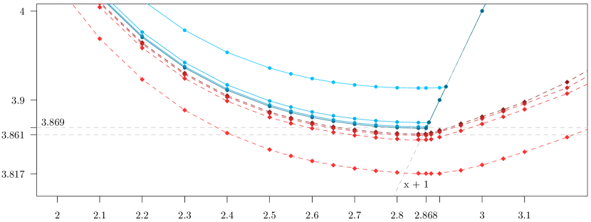
Figure 2: Visual representation of the computed bounds on the competitive ratio as functions of $\gamma$. Each data point corresponds to a single optimal solution of LP1 or LP2, the curves are interpolated. The blue (solid) curves correspond to the upper bound LP2 for $k=100$, $500$, $1000$ and $1500$ respectively. The red (dashed) curves represent the solutions of LP1 for the same steps of $k$. We obtain that our algorithm is $3.869$-competitive for $\gamma=2.868$ (1), and it is not better than $3.861$-competitive (4.2). Note that in line with results of Section 3, for a fixed value of $\gamma$, the value of $z_{k}(\gamma)$ increases with increasing $k$ while $y_{k}(\gamma)$, its upper bound, decreases with $k$.

Our computational results are summarized in Figure 2. We have been able to solve LPs with up to 1500 clients, which allows us to make the following two claims, one formally proved and one empirical:

Claim 1.

There exists an optimal solution for the linear program LP2 with parameters $k=1500$ and $\gamma=2.868$ of objective value $y_{1500}(2.868)\approx 3.869$.

Proof 4.1.

We provide the proof in the form of feasible LP solution and a feasible dual solution of the same objective value. The solutions are available along with the rest of our data at [13].

Empirical Claim 4.2.

The objective function $z_{1500}(\gamma)$ of LP1, viewed as a function of $\gamma$, is minimized for $\gamma\approx 2.867$ with objective value $z_{1500}(2.867)\approx 3.861$.

With 1, we can complete the proof of Theorem 1.1:

Proof 4.3 (Proof of Theorem 1.1).

We partition the cost of Opt into costs associated with a single facility that Opt opens, forming a star with the facility in the center. Lemma 3.1 gives us that $z_{k}(\gamma)$ is an upper bound on the competitive ratio of Algorithm 1 for a single star, and Corollary 3.9 implies that computing a single optimal solution of the upper bound LP2 is sufficient for the bound on competitive ratio. Finally, 1 tells us that for $\gamma=2.868$, the competitive ratio on a single star — and thus, on all stars — is, after rounding, at most $3.869$.

The complementary 4.2 provides a lower bound on the efficiency of our method, as it suggests that Algorithm 1 is not better than $3.861$-competitive, and thus our analysis is almost tight.

In Figure 2, we can see that all curves for LP2 begin to follow the line $y=x+1$ once they intersect it, which is not the case for the dashed curves of LP1. The following observation explains the structure of feasible solutions once the $y=x+1$ line is crossed.

Consider the linear program LP2 with parameters $k\geq 2$ and $\gamma$, and let us set $\mathrm{open}(f)+\sum_{i=0}^{k-1}(d_{i}+|a_{i}|)=1$. Then, there is a feasible solution to LP2 with objective value $\gamma+1$.

Proof 4.4.

Recall that LP2 is designed for the case the optimal solution opens a facility at time $\tau$, which we can think of as $0$. For our feasible solution, we set all distances to be identically zero and we release the first client at time $a_{0}=-1$, with $a_{1}=a_{2}=\cdots=a_{k-1}=0$. The cost of opening a facility is also zero. For the service times of the algorithm, we set $s_{0}=s_{1}=\cdots=s_{k-1}=0$.

We first double check that indeed, setting these values gives us $\mathrm{open}(f)+\sum_{i=0}^{k-1}(d_{i}+|a_{i}|)=1$; we now proceed to check that the solution is feasible. As all distances and service times are zero, all constrains except the type (2d) are trivially satisfied.

Let us restate the last set of constraints, (2d):

$$\sum_{i=\ell+1}^{k-1}\max{\{\gamma\cdot(s_{\ell}-a_{i})-d_{i},0\}}\leqslant\mathrm{open}(f) \forall_{\ell<k}.$$

Observe that $a_{0}$ does not appear in any constraint of this type, and so it is never checked that $\gamma(s_{0}-a_{0})\leqslant\mathrm{open}(f)=0$, which would be false for any $s_{0}>-1$. All constraints of this type only check variables $a_{1},\ldots,a_{k-1}$ and $s_{1},\ldots,s_{k-1}$, which are all set to zero, causing the constraints to be indeed satisfied.

The quirk from Section 4 does not cause any issues for us, as the minimum of $z_{k}(\gamma)$, which serves as a lower bound of the competitive ratio of Algorithm 1, is attained before the curve $z_{k}(\gamma)$ intersects $y=x+1$ (see Figure 2).

For our computations, we use the LP solver Gurobi Optimizer version 9 [32]. The source code of our generator and selected few solutions (that can be verified) can be found online at [13].

5 From Two-Sided to One-Sided Delay

We will now show how an online algorithm that solves the two-sided variant of the facility location problem can be transformed into an algorithm for the one-sided variant. We require that the former algorithm is $(\lambda,\xi)$-sensible for some constants $\lambda>1$ and $\xi>1$ (cf. Definition 2.2). Recall that by Lemma 2.3, Algorithm 1 is $(3/2,2)$-sensible for $\gamma=2$.

5.1 Algorithm definition

On the basis of an arbitrary online $(\lambda,\xi)$-sensible algorithm ATS for the two-sided variant, we construct an online algorithm for the one-sided variant in the following way.

Algorithm 2.

Our algorithm simulates the execution of ATS on the input instance, and when ATS opens a facility $f$ at point $y$ at time $\tau$, and connects a subset of clients to this facility, our algorithm does the same at time $\tau$.

From this point on, our algorithm tracks, in an online manner, all (late) connections to facility $f$. Clients that are already connected by ATS but not yet connected by our algorithm are called pending for $f$. At some times (defined below), our algorithm opens a new facility at $y$ (called a copy of $f$), and connects all clients pending for $f$ to this copy.

• Let $\tau+b$ be the earliest time when $p\cdot b\geqslant\mathrm{open}(y)$, where $p$ denotes the number of pending clients. (The inequality may be strict if it becomes true because of the increment of $p$.) If there are no pending clients at time $\tau+\mathrm{open}(y)$, we set $b=\mathrm{open}(y)$.

  In either case, the first copy of $f$ is opened at time $\tau+b$.

• Let

  $$\tilde{n}=\frac{\lambda\cdot\xi}{\lambda-1}\cdot\frac{\mathrm{open}(y)}{b}\,,$$

  Note that $\tilde{n}>1$ by the choice of $b$. Let $q=\sqrt{\log\tilde{n}}$ and let $\ell$ be the smallest integer such that $q^{\ell}>\tilde{n}$. Subsequent facility copies are opened at times $\tau+b\cdot q^{i}$ for all integers $i\in\{1,\ldots,\ell\}$.

In total, Algorithm 2 opens a facility at $y$ at time $\tau$, and $\ell+1$ of its copies at times $\tau+b\cdot q^{i}$, for $i\in\{0,\ldots,\ell\}$.

5.2 Analysis

In the following, we assume that ATS is $(\lambda,\xi)$-sensible for some fixed constants $\lambda>1$ and $\xi>1$. We show that Algorithm 2 is a valid algorithm (i.e., it eventually connects all clients), and we upper-bound its total cost in comparison to the cost paid by ATS.

We perform the cost comparison for each facility $f$ opened by ATS; in the following, we use $y$ to denote its location and $\tau$ to denote its opening time in the solution of ATS. We also use values of $b$, $\tilde{n}$, $q$ and $\ell$ as computed by Algorithm 2 when handling clients connected to $f$ by ATS.

Correctness

We start with the following helper claim.

Lemma 5.1.

It holds that $\tilde{n}\leqslant n\cdot\lambda\cdot\xi/(\lambda-1)$.

Proof 5.2.

Let $p^{\prime}$ be the number of clients ATS connected to $f$ within the interval $(\tau,\tau+b]$. If $p^{\prime}=0$, then $b=\mathrm{open}(y)$ and thus $\tilde{n}=(\lambda\cdot\xi)/(\lambda-1)$. The lemma follows trivially as $n\geqslant 1$. Otherwise, $p^{\prime}>0$, and then $p^{\prime}\cdot b\geqslant\mathrm{open}(y)$. In this case, $\tilde{n}=(\lambda\cdot\xi)\cdot(\lambda-1)^{-1}\cdot\mathrm{open}(y)/b\leqslant(\lambda\cdot\xi)\cdot(\lambda-1)^{-1}\cdot p^{\prime}$. As $p^{\prime}\leqslant n$, the lemma follows.

Lemma 5.3.

Algorithm 2 connects all clients.

Proof 5.4.

The last copy of the facility $f$ is opened by Algorithm 2 at time $\tau+b\cdot q^{\ell}$. Thus, it suffices to show that ATS connects no clients to $f$ after this time.

Fix any $t>0$, any integer $i\geqslant 0$, and consider time interval

$$I^{t}_{i}=\Big{(}\tau+\lambda^{i}\cdot t,\;\tau+\lambda^{i+1}\cdot t\Big{]}.$$

As ATS is $(\lambda,\xi)$-sensible, it connects at most $\xi\cdot\mathrm{open}(y)/(\lambda^{i}\cdot t)$ clients within interval $I^{t}_{i}$.

Note that $\biguplus_{i=0}^{\infty}I^{t}_{i}=(\tau+\lambda^{0}\cdot t,\infty)=(\tau+t,\infty)$. Thus, for an arbitrary $t$, by summing over all $i\geqslant 0$, the number of clients connected after time $\tau+t$ is at most

$$\sum_{i=0}^{\infty}\frac{\xi\cdot\mathrm{open}(y)}{\lambda^{i}\cdot t}=\frac{\lambda\cdot\xi}{\lambda-1}\cdot\frac{\mathrm{open}(y)}{t}=\frac{\tilde{n}\cdot b}{t}\,.$$

Hence, the number of clients connected after time $\tau+b\cdot q^{\ell}$ is at most $\tilde{n}\cdot b/(b\cdot q^{\ell})=\tilde{n}/q^{\ell}<1$. As the number of clients is integral, it must be zero.

Bounding the waiting time

Now we focus on bounding the total waiting time of Algorithm 2. Let $C$ be the set of clients connected by ATS to the facility $f$ at $y$. We split $C$ into four disjoint parts: the clients connected by ATS at time $\tau$, within interval $(\tau,\tau+b)$, at time $\tau+b$, and after $\tau+b$. We denote these parts $C_{=\tau}$, $C_{(\tau,\tau+b)}$, $C_{=\tau+b}$ and $C_{>\tau+b}$, respectively. For any client $j\in C$, let $w^{\mathrm{ATS}}_{j}$ and $w_{j}$ denote its waiting cost in the solutions of ATS and Algorithm 2, respectively.

Lemma 5.5.

For any client $j\in C\setminus C_{(\tau,\tau+b)}$, it holds that $w_{j}\leqslant q\cdot w^{\mathrm{ATS}}_{j}$.

Proof 5.6.

For any client $j$, let $t_{j}$ be the time of its arrival and $t^{c}_{j}$ the time ATS connects it to facility $f$.

In the case $j\in C_{=\tau}$, in both solutions of ATS and Algorithm 2, client $j$ waits till $\tau$, and thus $w_{j}=w^{\mathrm{ATS}}_{j}$. The case $j\in C_{=\tau+b}$ is possible only if $t_{j}=\tau+b$, and then $w_{j}=0\leqslant q\cdot w^{\mathrm{ATS}}_{j}$.

It remains to consider the case $j\in C_{>\tau+b}$, i.e., $t^{c}_{j}>\tau+b$. Let $w^{\mathrm{init}}_{j}=t^{c}_{j}-t_{j}$; this amount represents the inevitable waiting time that $j$ incurs in both solutions. Note that $w^{\mathrm{ATS}}_{j}-w^{\mathrm{init}}_{j}=t^{c}_{j}-\tau$ corresponds to the facility-side waiting cost of $j$ in the solution of ATS. By Lemma 5.3, $t^{c}_{j}\leqslant\tau+b\cdot q^{\ell}$. Thus, there exists an integer $i\in\{1,\ldots,\ell\}$, such that $\tau+b\cdot q^{i-1}<t^{c}_{j}\leqslant\tau+b\cdot q^{i}$. Algorithm 2 connects $j$ at time $\tau+b\cdot q^{i}$, and therefore

$$w_{j}-w^{\mathrm{init}}_{j}=\tau+b\cdot q^{i}-t^{c}_{j}\leqslant b\cdot q^{i}=q\cdot\left(b\cdot q^{i-1}\right)<q\cdot(t^{c}_{j}-\tau)=q\cdot(w^{\mathrm{ATS}}_{j}-w^{\mathrm{init}})\,.$$

The proof is concluded by adding $w^{\mathrm{init}}_{j}$ to both sides.

Lemma 5.7.

It holds that $\sum_{c\in C}w(c)\leqslant\mathrm{open}(y)+q\cdot\sum_{c\in C}w^{\mathrm{ATS}}(c)$.

Proof 5.8.

We use the same notions of $t_{j}$, $t^{c}_{j}$, $w_{j}$, $w^{\mathrm{ATS}}_{j}$ and $w^{\mathrm{init}}_{j}$ as in the previous proof.

Fix any client $j\in C_{(\tau,\tau+b)}$. Clearly, $t^{c}_{j}>\tau$. Furthermore, $j$ is served by Algorithm 2 at time $\tau+b$, and thus

$$\sum_{j\in C_{(\tau,\tau+b)}}\left(w_{j}-w^{\mathrm{init}}_{j}\right)=\sum_{j\in C_{(\tau,\tau+b)}}\left(\tau+b-t_{j}^{c}\right)\leqslant|C_{(\tau,\tau+b)}|\cdot b<\mathrm{open}(y)\,.$$

The last inequality follows by the definition of $b$ in Algorithm 2. By adding $\sum_{c\in C_{(\tau,\tau+b)}}w^{\mathrm{init}}_{j}$ to both sides, we obtain

$$\sum_{j\in C_{(\tau,\tau+b)}}w_{j}\leqslant\mathrm{open}(y)+\sum_{j\in C_{(\tau,\tau+b)}}w^{\mathrm{init}}_{j}\leqslant\mathrm{open}(y)+\sum_{j\in C_{(\tau,\tau+b)}}w^{\mathrm{ATS}}_{j}\,.$$

By combining the inequality above with Lemma 5.5 applied to all $C\setminus C_{(\tau,\tau+b)}$, we obtain the lemma statement.

Competitive ratio

Finally, we use our bounds to prove Theorem 1.2, i.e., show that the competitive ratio of Algorithm 2.

Proof 5.9 (Proof of Theorem 1.2).

We fix any $(\lambda,\xi)$-sensible $O(1)$-competitive algorithm ATS for the two-sided variant. By Lemma 2.3, such algorithm exists for $\lambda=3/2$ and $\xi=2$.

We fix any facility opened by ATS at location $y$; let $C$ denote the set of clients that are connected to this facility in the solution of ATS. Below we show that the total cost pertaining to clients from $C$ in the solution of Algorithm 2 is at most $O(\log n/\log\log n)$ times larger than the cost pertaining to these clients in the solution of ATS.

The theorem will then follow by summing this relation over all facilities opened by ATS, and observing that the value of Opt for the one-sided variant can be only more expensive than Opt for the two-sided variant (as the two-sided variant is a relaxation of the one-sided variant).

We relate parts of cost of solution produced by Algorithm 2 to the corresponding costs of ATS.

• The cost of connecting clients from $C$ by Algorithm 2 is trivially equal to the connection cost in the solution of ATS.

• To bound the waiting cost of clients from $C$, we apply Lemma 5.7 obtaining that $\sum_{c\in C}w(c)\leqslant\mathrm{open}(y)+q\cdot\sum_{c\in C}w^{\mathrm{ATS}}(c)$. As $q=\sqrt{\log\tilde{n}}=O(\sqrt{\log n})=O(\log n/\log\log n)$, the total waiting cost of Algorithm 2 is at most $\mathrm{open}(y)+O(\log n/\log\log n)\cdot\sum_{c\in C}w^{\mathrm{ATS}}(c)$.

• Algorithm 2 opens a facility at location $y$ at time $\tau$ and then $\ell+1$ of its copies at times $\tau+b\cdot q^{i}$ for $i\in\{0,\ldots,\ell\}$. Thus, its overall opening cost is $(\ell+2)\cdot\mathrm{open}(y)$. Recall that $\ell=\lceil\log\tilde{n}/\log q\rceil=O(\log\tilde{n}/\log\log\tilde{n})$. By Lemma 5.1, the latter amount is $O(\log n/\log\log n)$. Thus, the opening cost of Algorithm 2 is $O(\log n/\log\log n)\cdot\mathrm{open}(y)$ while that of ATS is $\mathrm{open}(y)$.

The proof follows by adding guarantees of all the cases above.

References

- [1] Karen Aardal, Jaroslaw Byrka, and Mohammad Mahdian. Facility location. In Encyclopedia of Algorithms, pages 717–724. Springer, 2016. doi:10.1007/978-1-4939-2864-4\_139.
- [2] Aris Anagnostopoulos, Russell Bent, Eli Upfal, and Pascal Van Hentenryck. A simple and deterministic competitive algorithm for online facility location. Information and Computation, 194(2):175–202, 2004. doi:10.1016/j.ic.2004.06.002.
- [3] Itai Ashlagi, Yossi Azar, Moses Charikar, Ashish Chiplunkar, Ofir Geri, Haim Kaplan, Rahul M. Makhijani, Yuyi Wang, and Roger Wattenhofer. Min-cost bipartite perfect matching with delays. In Proc. 20th Approximation, Randomization, and Combinatorial Optimization. Algorithms and Techniques (APPROX/RANDOM), pages 1:1–1:20, 2017.
- [4] Yossi Azar, Ashish Chiplunkar, and Haim Kaplan. Polylogarithmic bounds on the competitiveness of min-cost perfect matching with delays. In Proc. 28th ACM-SIAM Symp. on Discrete Algorithms (SODA), pages 1051–1061, 2017.
- [5] Yossi Azar, Ashish Chiplunkar, Shay Kutten, and Noam Touitou. Set cover with delay — clairvoyance is not required. In Proc. 28th European Symp. on Algorithms (ESA), pages 8:1–8:21, 2020. doi:10.4230/LIPIcs.ESA.2020.8.
- [6] Yossi Azar and Amit Jacob Fanani. Deterministic min-cost matching with delays. Theory of Computing Systems, 64(4):572–592, 2020. doi:10.1007/s00224-019-09963-7.
- [7] Yossi Azar, Arun Ganesh, Rong Ge, and Debmalya Panigrahi. Online service with delay. In Proc. 49th ACM Symp. on Theory of Computing (STOC), pages 551–563, 2017.
- [8] Yossi Azar, Runtian Ren, and Danny Vainstein. The min-cost matching with concave delays problem. In Proc. 2021 ACM-SIAM Symp. on Discrete Algorithms (SODA), pages 301–320, 2021. doi:10.1137/1.9781611976465.20.
- [9] Yossi Azar and Noam Touitou. General framework for metric optimization problems with delay or with deadlines. In Proc. 60th IEEE Symp. on Foundations of Computer Science (FOCS), pages 60–71, 2019. doi:10.1109/FOCS.2019.00013.
- [10] Yossi Azar and Noam Touitou. Beyond tree embeddings - a deterministic framework for network design with deadlines or delay. In Proc. 61st IEEE Symp. on Foundations of Computer Science (FOCS), pages 1368–1379, 2020. doi:10.1109/FOCS46700.2020.00129.
- [11] Marcin Bienkowski, Martin Böhm, Jaroslaw Byrka, Marek Chrobak, Christoph Dürr, Lukáš Folwarczný, Lukasz Jez, Jirí Sgall, Nguyen Kim Thang, and Pavel Veselý. Online algorithms for multilevel aggregation. Operations Research, 68(1):214–232, 2020. doi:10.1287/opre.2019.1847.
- [12] Marcin Bienkowski, Martin Böhm, Jaroslaw Byrka, Marek Chrobak, Christoph Dürr, Lukáš Folwarczný, Lukasz Jez, Jirí Sgall, Nguyen Kim Thang, and Pavel Veselý. New results on multi-level aggregation. Theoretical Computer Science, 861:133–143, 2021. doi:10.1016/j.tcs.2021.02.016.
- [13] Marcin Bienkowski, Martin Böhm, Jarosław Byrka, and Jan Marcinkowski. Data and computations for online facility location with linear delay. https://github.com/bohm/fl-double-sided-waiting, 2021.
- [14] Marcin Bienkowski, Jaroslaw Byrka, Marek Chrobak, Łukasz Jeż, Dorian Nogneng, and Jirí Sgall. Better approximation bounds for the joint replenishment problem. In Proc. 25th ACM-SIAM Symp. on Discrete Algorithms (SODA), pages 42–54, 2014.
- [15] Marcin Bienkowski, Jaroslaw Byrka, Marek Chrobak, Łukasz Jeż, Jiři Sgall, and Grzegorz Stachowiak. Online control message aggregation in chain networks. In Proc. 13th Int. Workshop on Algorithms and Data Structures (WADS), pages 133–145, 2013.
- [16] Marcin Bienkowski, Artur Kraska, Hsiang-Hsuan Liu, and Pawel Schmidt. A primal-dual online deterministic algorithm for matching with delays. In Proc. 16th Workshop on Approximation and Online Algorithms (WAOA), pages 51–68, 2018. doi:10.1007/978-3-030-04693-4\_4.
- [17] Marcin Bienkowski, Artur Kraska, and Paweł Schmidt. A match in time saves nine: Deterministic online matching with delays. In Proc. 15th Workshop on Approximation and Online Algorithms (WAOA), pages 132–146, 2017.
- [18] Marcin Bienkowski, Artur Kraska, and Paweł Schmidt. Online service with delay on a line. In Proc. 25th Int. Colloq. on Structural Information and Communication Complexity (SIROCCO), pages 237–248, 2018. doi:10.1007/978-3-030-01325-7\_22.
- [19] Niv Buchbinder, Moran Feldman, Joseph (Seffi) Naor, and Ohad Talmon. O(depth)-competitive algorithm for online multi-level aggregation. In Proc. 28th ACM-SIAM Symp. on Discrete Algorithms (SODA), pages 1235–1244, 2017.
- [20] Niv Buchbinder, Tracy Kimbrel, Retsef Levi, Konstantin Makarychev, and Maxim Sviridenko. Online make-to-order joint replenishment model: Primal-dual competitive algorithms. Operations Research, 61(4):1014–1029, 2013. doi:10.1287/opre.2013.1188.
- [21] Jaroslaw Byrka and Karen Aardal. An optimal bifactor approximation algorithm for the metric uncapacitated facility location problem. SIAM Journal on Computing, 39(6):2212–2231, 2010. doi:10.1137/070708901.
- [22] Rodrigo A. Carrasco, Kirk Pruhs, Cliff Stein, and José Verschae. The online set aggregation problem. In Proc. 13th Latin American Theoretical Informatics Symposium (LATIN), pages 245–259, 2018. doi:10.1007/978-3-319-77404-6\_19.
- [23] Moses Charikar and Sudipto Guha. Improved combinatorial algorithms for facility location problems. SIAM Journal on Computing, 34(4):803–824, 2005. doi:10.1137/S0097539701398594.
- [24] Marek Chrobak. Online aggregation problems. SIGACT News, 45(1):91–102, 2014.
- [25] Fabián A. Chudak and David B. Shmoys. Improved approximation algorithms for the uncapacitated facility location problem. SIAM Journal on Computing, 33(1):1–25, 2003. doi:10.1137/S0097539703405754.
- [26] Daniel R. Dooly, Sally A. Goldman, and Stephen D. Scott. On-line analysis of the TCP acknowledgment delay problem. Journal of the ACM, 48(2):243–273, 2001.
- [27] Yuval Emek, Shay Kutten, and Roger Wattenhofer. Online matching: haste makes waste! In Proc. 48th ACM Symp. on Theory of Computing (STOC), pages 333–344, 2016.
- [28] Yuval Emek, Yaacov Shapiro, and Yuyi Wang. Minimum cost perfect matching with delays for two sources. Theoretical Computer Science, 754:122–129, 2019. doi:10.1016/j.tcs.2018.07.004.
- [29] Dimitris Fotakis. A primal-dual algorithm for online non-uniform facility location. Journal of Discrete Algorithms, 5(1):141–148, 2007. doi:10.1016/j.jda.2006.03.001.
- [30] Dimitris Fotakis. On the competitive ratio for online facility location. Algorithmica, 50(1):1–57, 2008. doi:10.1007/s00453-007-9049-y.
- [31] Sudipto Guha and Samir Khuller. Greedy strikes back: Improved facility location algorithms. Journal of Algorithms, 31(1):228–248, 1999. doi:10.1006/jagm.1998.0993.
- [32] Gurobi Optimization, LLC. Gurobi Optimizer Reference Manual, 2021. URL: https://www.gurobi.com.
- [33] Kamal Jain, Mohammad Mahdian, Evangelos Markakis, Amin Saberi, and Vijay V. Vazirani. Greedy facility location algorithms analyzed using dual fitting with factor-revealing LP. Journal of the ACM, 50(6):795–824, 2003. doi:10.1145/950620.950621.
- [34] Kamal Jain, Mohammad Mahdian, and Amin Saberi. A new greedy approach for facility location problems. In Proc. 34th ACM Symp. on Theory of Computing (STOC), pages 731–740, 2002. doi:10.1145/509907.510012.
- [35] Anna R. Karlin, Claire Kenyon, and Dana Randall. Dynamic TCP acknowledgement and other stories about e/(e - 1). Algorithmica, 36(3):209–224, 2003.
- [36] Madhukar R. Korupolu, C. Greg Plaxton, and Rajmohan Rajaraman. Analysis of a local search heuristic for facility location problems. Journal of Algorithms, 37(1):146–188, 2000. doi:10.1006/jagm.2000.1100.
- [37] Shi Li. A 1.488 approximation algorithm for the uncapacitated facility location problem. Information and Computation, 222:45–58, 2013. doi:10.1016/j.ic.2012.01.007.
- [38] Xingwu Liu, Zhida Pan, Yuyi Wang, and Roger Wattenhofer. Impatient online matching. In Proc. 29th Int. Symp. on Algorithms and Computation (ISAAC), pages 62:1–62:12, 2018. doi:10.4230/LIPIcs.ISAAC.2018.62.
- [39] Mohammad Mahdian, Yinyu Ye, and Jiawei Zhang. Approximation algorithms for metric facility location problems. SIAM Journal on Computing, 36(2):411–432, 2006. doi:10.1137/S0097539703435716.
- [40] Adam Meyerson. Online facility location. In Proc. 42nd IEEE Symp. on Foundations of Computer Science (FOCS), pages 426–431, 2001. doi:10.1109/SFCS.2001.959917.
- [41] David B. Shmoys, Éva Tardos, and Karen Aardal. Approximation algorithms for facility location problems (extended abstract). In Proc. 29th ACM Symp. on Theory of Computing (STOC), pages 265–274, 1997. doi:10.1145/258533.258600.
- [42] Michael A. Stanko and David H. Henard. How crowdfunding influences innovation. MIT Sloan Management Review, 57(3):15, 2016.