Mapping conditional distributions for domain adaptation under generalized target shift

Abstract

We consider the problem of unsupervised domain adaptation (UDA) between a source and a target domain under conditional and label shift a.k.a Generalized Target Shift (GeTarS). Unlike simpler UDA settings, few works have addressed this challenging problem. Recent approaches learn domain-invariant representations, yet they have practical limitations and rely on strong assumptions that may not hold in practice. In this paper, we explore a novel and general approach to align pretrained representations, which circumvents existing drawbacks. Instead of constraining representation invariance, it learns an optimal transport map, implemented as a NN, which maps source representations onto target ones. Our approach is flexible and scalable, it preserves the problem’s structure and it has strong theoretical guarantees under mild assumptions. In particular, our solution is unique, matches conditional distributions across domains, recovers target proportions and explicitly controls the target generalization risk. Through an exhaustive comparison on several datasets, we challenge the state-of-the-art in GeTarS.

1 Introduction

Unsupervised Domain Adaptation (UDA) methods (Pan & Yang, 2010) train a classifier with labelled samples from a source domain $S$ such that its risk on an unlabelled target domain $T$ is low. This problem is ill-posed and simplifying assumptions were considered. Initial contributions focused on three settings which decompose differently the joint distribution over input and label $X\times Y$: covariate shift (CovS) (Shimodaira, 2000) with $p_{S}(Y|X)=p_{T}(Y|X)$, $p_{S}(X)\neq p_{T}(X)$, target shift (TarS) (Zhang et al., 2013) with $p_{S}(Y)\neq p_{T}(Y)$, $p_{S}(X|Y)=p_{T}(X|Y)$ and conditional shift (Zhang et al., 2013) with $p_{S}(X|Y)\neq p_{T}(X|Y),p_{S}(Y)=p_{T}(Y)$. These assumptions are restrictive for real-world applications and were extended into model shift when $p_{S}(Y|X)\neq p_{T}(Y|X)$, $p_{S}(X)\neq p_{T}(X)$ (Wang & Schneider, 2014; 2015) and generalized target shift (GeTarS) (Zhang et al., 2013) when $p_{S}(X|Y)\neq p_{T}(X|Y),p_{S}(Y)\neq p_{T}(Y)$. We consider GeTarS where a key challenge is to map the source domain onto the target one to minimize both conditional and label shifts, without using target labels. The current SOTA in Gong et al. (2016); Combes et al. (2020); Rakotomamonjy et al. (2021); Shui et al. (2021) learns domain-invariant representations and uses estimated class-ratios between domains as importance weights in the training loss. However, this approach has several limitations. First, it updates representations through adversarial alignment which is prone to well-known instabilities, especially on applications where there is no established Deep Learning architectures e.g. click-through-rate prediction, spam filtering etc. in contrast to vision. Second, to transfer representations, the domain-invariance constraint breaks the original problem structure and it was shown that this may degrade the discriminativity of target representations (Liu et al., 2019). Existing approaches that consider this issue (Xiao et al., 2019; Li et al., 2020; Chen et al., 2019) were not applied to GeTarS. Finally, generalization guarantees are derived under strong assumptions, detailed in Section 2.3, which may not hold in practice.

In this paper, we address these limitations with a new general approach, named Optimal Sample Transformation and Reweight (OSTAR), which maps pretrained representations using Optimal Transport (OT). OSTAR proposes an alternative to constraining representation invariance and performs jointly three operations: given a pretrained encoder, (i) it learns an OT map, implemented as a neural network (NN), between encoded source and target conditionals, (ii) it estimates target proportions for sample reweighting and (iii) it learns a classifier for the target domain using source labels. OSTAR has several benefits: (i) it is flexible, scalable and preserves target discriminativity and (ii) it provides strong theoretical guarantees under mild assumptions. In summary, our contributions are:

• We propose an approach, OSTAR, to align pretrained representations under GeTarS. Without constraining representation-invariance, OSTAR jointly learns a classifier for inference on the target domain and an OT map, which maps representations of source conditionals to those of target ones under class-reweighting. OSTAR preserves target discriminativity and experimentally challenges the state-of-the-art for GeTarS.

• OSTAR implements its OT map as a NN shared across classes. Our approach is thus flexible and has native regularization biases for stability. Moreover it is scalable and generalizes beyond training samples unlike standard linear programming based OT approaches.

• OSTAR has strong theoretical guarantees under mild assumptions: its solution is unique, recovers target proportions and correctly matches source and target conditionals at the optimum. It also explicitly controls the target risk with a new Wasserstein-based bound.

Our paper is organized as follows. In Section 2, we define our problem, approach and assumptions. In Section 3, we derive theoretical results. In Section 4, we describe our implementation. We report in Section 5 experimental results and ablation studies. In Section 6, we present related work.

2 Proposed approach

In this section, we successively define our problem, present our method, OSTAR and its main ideas and introduce our assumptions, used to provide theoretical guarantees for our method.

2.1 Problem definition

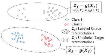
Denoting $\mathcal{X}$ the input space and $\mathcal{Y}=\{1,\ldots,K\}$ the label space, we consider UDA between a source $S=(\mathcal{X}_{S},\mathcal{Y}_{S},p_{S}(X,Y))$ with labeled samples $\widehat{S}=\{(\mathbf{x}_{S}^{(i)},y_{S}^{(i)})\}_{i=1}^{n}\in(\mathcal{X}_{S}\times\mathcal{Y}_{S})^{n}$ and a target $T=(\mathcal{X}_{T},\mathcal{Y}_{T},p_{T}(X,Y))$ with unlabeled samples $\widehat{T}=\{\mathbf{x}_{T}^{(i)}\}_{i=1}^{m}\in\mathcal{X}_{T}^{m}$. We denote $\mathcal{Z}\subset\mathbb{R}^{d}$ a latent space and $g:\mathcal{X}\rightarrow\mathcal{Z}$ an encoder from $\mathcal{X}$ to $\mathcal{Z}$. $\mathcal{Z}_{S}$ and $\mathcal{Z}_{T}$ are the encoded source and target input domains, $\mathcal{Z}_{\widehat{S}}$ and $\mathcal{Z}_{\widehat{T}}$ the corresponding training sets and $Z$ a random variable in this space. The latent marginal probability induced by $g$ on $D\in\{S,T\}$ is defined as $\forall A\subset\mathcal{Z},p_{D}^{g}(A)\triangleq g_{\#}(p_{D}(A))$. For convenience, $\bm{p}_{D}^{Y}\in\mathbb{R}^{K}$ denotes the label marginal $p_{D}(Y)$ and $p_{D}(Z)\triangleq p_{D}^{g}(Z)$. In all generality, latent conditional distributions and label marginals differ across domains; this is the GeTarS assumption (Zhang et al., 2013) made in feature space $\mathcal{Z}$ rather than input space $\mathcal{X}$, as in Definition 1. GeTarS is illustrated in Figure LABEL:fig:getars and states that representations from a given class are different across domains with different label proportions. Operating in the latent space has several practical advantages e.g. improved discriminativity and dimension reduction.

Definition 1 (GeTarS).

GeTarS is characterized by conditional mismatch across domains i.e. $\exists j\in\{1,\ldots,K\},p_{S}(Z|Y=j)\neq p_{T}(Z|Y=j)$ and label shift i.e. $\bm{p}_{S}^{Y}\neq\bm{p}_{T}^{Y}$.

Our goal is to learn a classifier in $\mathcal{Z}$ with low target risk, using source labels. This is challenging as (i) target labels are unknown and (ii) there are two shifts to handle. We will show that this can be achieved with pretrained representations if we recover two key properties: (i) a map which matches source and target conditional distributions and (ii) target proportions to reweight samples by class-ratios and thus account for label shift. Our approach, OSTAR, achieves this objective.

2.2 Mapping conditional distributions under label shift

We now present the components in OSTAR, their objective and the various training steps.

Components

The main components of OSTAR, illustrated in Figure LABEL:fig:star, are detailed below. These components are learned and estimated using the algorithm detailed in Section 4. They include:

• a fixed encoder $g:\mathcal{X}\rightarrow\mathcal{Z}$, defined in Section 2.1.

• a mapping $\phi:\mathcal{Z}\rightarrow\mathcal{Z}$, acting on source samples encoded by $g$.

• a label proportion vector $\bm{p}_{N}^{Y}$ on the simplex $\Delta_{K}$.

• a classifier $f_{N}:\mathcal{Z}\rightarrow\{1,\ldots,K\}$ for the target domain in a hypothesis class $\mathcal{H}$ over $\mathcal{Z}$.

Objective

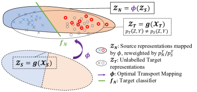
$g$ encodes source and target samples in a latent space such that it preserves rich information about the target task and such that the risk on the source domain is small. $g$ is fixed throughout training to preserve target discriminativity. $\phi$ should map encoded source conditionals in $\mathcal{Z}_{S}$ onto corresponding encoded target ones in $\mathcal{Z}_{T}$ to account for conditional shift; $\mathcal{Z}_{N}$ denotes the mapped space. $\bm{p}_{N}^{Y}$ should estimate the target proportions $\bm{p}_{T}^{Y}$ to account for label shift. Components $(\phi,\bm{p}_{N}^{Y})$ define a new labelled domain in latent space $N=(\mathcal{Z}_{N},\mathcal{Y}_{N},p_{N}(Z,Y))$ through a Sample Transformation And Reweight operation of the encoded $S$ domain, as illustrated in Figure LABEL:fig:star. Indeed, the pushforward by $\phi$ of encoded source conditionals defines conditionals in domain $N$, $p_{N}^{\phi}(Z|Y)$:

$$\forall k,~{}p_{N}^{\phi}(Z|Y=k)\triangleq\phi_{\#}\Big{(}p_{S}(Z|Y=k)\Big{)}\ref{note1}$$

Then, $\bm{p}_{N}^{Y}$ weights each conditional in $N$. This yields a marginal distribution in $N$, $p_{N}^{\phi}(Z)$:

$$p_{N}^{\phi}(Z)\triangleq\sum_{k=1}^{K}\bm{p}_{N}^{Y=k}p_{N}^{\phi}(Z|Y=k)$$ (1)

Finally, classifier $f_{N}$ is trained on labelled samples from domain $N$. This is possible as each sample in $N$ is a projection of a labelled sample from $S$. $f_{N}$ can then be used for inference on $T$. We will show that it has low target risk when components $\phi$ and $\bm{p}_{N}^{Y}$ achieve their objectives detailed above.

(a)

(b)

Figure 1: Illustration of our approach on a 2-class UDA problem [better viewed in color]. (a) A pretrained encoder $g$ defines a latent space $\mathcal{Z}$ with labelled source samples ${\color[rgb]{0,0,1}\definecolor[named]{pgfstrokecolor}{rgb}{0,0,1}\times}{\color[rgb]{1,0,0}\definecolor[named]{pgfstrokecolor}{rgb}{1,0,0}\circ}$ and unlabelled target samples ${\color[rgb]{.5,.5,.5}\definecolor[named]{pgfstrokecolor}{rgb}{.5,.5,.5}\pgfsys@color@gray@stroke{.5}\pgfsys@color@gray@fill{.5}\times\circ}$ under conditional and label shift (GeTarS). (b) We train a target classifier ${\color[rgb]{0.1328125,0.546875,0.1328125}\definecolor[named]{pgfstrokecolor}{rgb}{0.1328125,0.546875,0.1328125}f_{N}}$ on a new domain $N$, where labelled samples ${\color[rgb]{0.68,0.85,0.9}\definecolor[named]{pgfstrokecolor}{rgb}{0.68,0.85,0.9}\times}{\color[rgb]{1,0,0}\definecolor[named]{pgfstrokecolor}{rgb}{1,0,0}\bm{\circ}}$ are obtained by (i) mapping source samples with ${\color[rgb]{0.6,0.4,0.8}\definecolor[named]{pgfstrokecolor}{rgb}{0.6,0.4,0.8}\phi}$ acting on conditional distributions and (ii) reweighting these samples by estimated class-ratios $\bm{p}_{N}^{Y}/\bm{p}_{S}^{Y}$. ${\color[rgb]{0.6,0.4,0.8}\definecolor[named]{pgfstrokecolor}{rgb}{0.6,0.4,0.8}\phi}$ should match source and target conditionals and $\bm{p}_{N}^{Y}$ should estimate target proportions $\bm{p}_{T}^{Y}$.

Training

We train OSTAR’s components in two stages. First, we train $g$ along a source classifier $f_{S}$ from scratch by minimizing source classification loss; alternatively, $g$ can be tailored to specific problems with pretraining. Second, we jointly learn $(f_{N},\phi,\bm{p}_{N}^{Y})$ to minimize a classification loss in domain $N$ and to match target conditionals and proportions with those in domain $N$. As target conditionals and proportions are unknown, we propose a proxy problem for $(\phi,\bm{p}_{N}^{Y})$ to match instead latent marginals $p_{T}(Z)$ and $p_{N}^{\phi}(Z)$ (1). We solve this proxy problem under least action principle measured by a Monge transport cost (Santambrogio, 2015), denoted $\mathcal{C}(\phi)$, as in problem (OT):

$$\min_{\phi,\bm{p}_{N}^{Y}\in\Delta_{K}}\mathcal{C}(\phi)\triangleq\sum_{k=1}^{K}\int_{\mathbf{z}\in\mathcal{Z}}\|\phi(\mathbf{z})-\mathbf{z}\|_{2}^{2}~{}p_{S}(\mathbf{z}|Y=k)d\mathbf{z}$$ (OT)

$$\text{subject to~{}}p_{N}^{\phi}(Z)=p_{T}(Z)$$

For any function $\phi$ e.g. parametrized by a NN, $\mathcal{C}(\phi)$ is the transport cost of encoded source conditionals by $\phi$. It uses a cost function, $c(\mathbf{x},\mathbf{y})=\|\mathbf{x}-\mathbf{y}\|_{2}^{p}$, where without loss of generality $p=2$. The optimal $\mathcal{C}(\phi)$ is the sum of Wasserstein-2 distances between source conditionals and their mappings. Problem (OT) seeks to minimize $\mathcal{C}(\phi)$ under marginal matching. We provide some further background on optimal transport in Appendix C and discuss there the differences between our OT problem (OT) and the standard Monge OT problem between $p_{S}(Z)$ and $p_{T}(Z)$.

Our OT formulation is key to the approach. First, it is at the basis of our theoretical analysis. Under Assumption 2 later defined, the optimal transport cost is the sum of the Wasserstein-2 distance between source and matched target conditionals. We can then provide conditions on these distances in Assumption 3 to formally define when the solution to problem (OT) correctly matches conditionals. Second, it allows us to learn the OT map with a NN. This NN approach: (i) generalizes beyond training samples and scales up with the number of samples unlike linear programming based OT approaches (Courty et al., 2017b) and (ii) introduces useful stability biases which make learning less prone to numerical instabilities as highlighted in de Bézenac et al. (2021); Karkar et al. (2020).

2.3 Assumptions

In Section 3 we will introduce the theoretical properties of our method which offers several guarantees. As always, this requires some assumptions which are introduced below. We discuss their relations with assumptions used in related work and detail why they are less restrictive. We provide some additional discussion on their motivation and validity in Appendix D.

Assumption 1 (Cluster Assumption on S).

$\forall k,\bm{p}_{S}^{Y=k}>0$ and there is a partition of the source domain $\mathcal{Z}_{S}$ such that $\mathcal{Z}_{S}=\cup_{k=1}^{K}\mathcal{Z}_{S}^{(k)}$ and $\forall k~{}p_{S}(Z\in\mathcal{Z}_{S}^{(k)}|Y=k)=1$.

Assumption 1, inspired from Chapelle et al. (2010), states that source representations with the same label are within the same cluster. It helps guarantee that only one map is required to match source and target conditionals. Assumption 1 is for instance satisfied when the classification loss on the source domain is zero which corresponds to the training criterion of our encoder $g$. Interestingly other approaches e.g. Combes et al. (2020); Rakotomamonjy et al. (2021) assume that it also holds for target representations; this is harder to induce as target labels are unknown.

Assumption 2 (Conditional matching).

A mapping $\phi$ solution to our matching problem in problem (OT) maps a source conditional to a target one i.e. $\forall k~{}\exists j~{}\phi_{\#}(p_{S}(Z|Y=k))=p_{T}(Z|Y=j)$.

Assumption 2 guarantees that mass of a source conditional will be entirely transferred to a target conditional; $\phi$ solution to problem (OT) will then perform optimal assignment between conditionals. It is less restrictive than alternatives: the ACons assumption in Zhang et al. (2013); Gong et al. (2016) states the existence of a map matching the right conditional pairs i.e. $j=k$ in Assumption 2, while the GLS assumption of Combes et al. (2020) imposes that $p_{S}(Z|Y)=p_{T}(Z|Y)$. GLS is thus included in Assumption 2 when $j=k$ and $\phi=\mathrm{Id}$ and is more restrictive.

Assumption 3 (Cyclical monotonicity between S and T).

For all $K$ elements permutation $\sigma$, conditional probabilities in the source and target domains satisfy $\sum_{k=1}^{K}\mathcal{W}_{2}(p_{S}(Z|Y=k),p_{T}(Z|Y=k))\leq\sum_{k=1}^{K}\mathcal{W}_{2}(p_{S}(Z|Y=k),p_{T}(Z|Y=\sigma(k))$ with $\mathcal{W}_{2}$, the Wasserstein-2 distance.

Assumption 3, introduced in Rakotomamonjy et al. (2021), formally defines settings where conditionals are guaranteed to be correctly matched with an optimal assignment in the latent space under Assumption 2. One sufficient condition for yielding this assumption is when $\forall k,j,~{}\mathcal{W}_{2}(p_{S}(Z|Y=k),p_{T}(Z|Y=k))\leq\mathcal{W}_{2}(p_{S}(Z|Y=k),p_{T}(Z|Y=j))$. This last condition is typically achieved when conditionals between source and target of the same class are “sufficiently near” to each other.

Assumption 4 (Conditional linear independence on T).

$\{p_{T}(Z|Y=k)\}_{k=1}^{K}$ are linearly independent implying $\forall k,\not\exists\alpha\in\left\{\Delta_{K}|~{}p_{T}(Z|Y=k)=\sum_{j=1,j\neq k}^{K}\alpha_{j}p_{T}(Z|Y=j)\right\}$.

Assumption 4 is standard and seen in TarS to guarantee correctly estimating target proportions (Redko et al., 2019; Garg et al., 2020). It discards pathological cases like when $\exists(i,j,k)\,\exists(a,b)~{}s.t.~{}a+b=1,p_{T}(Z|Y=i)=a\times p_{T}(Z|Y=j)+b\times p_{T}(Z|Y=k)$. It is milder than its alternative A2Cons in Zhang et al. (2013); Gong et al. (2016) which states linear independence of linear combinations of source and target conditionals, in $\mathcal{X}$ respectively $\mathcal{Z}$.

3 Theoretical results

We present our theoretical results, with proofs in Appendix E, for OSTAR under our mild assumptions in Section 2.3. We first analyze in Section 3.1 the properties of the solution to our problem in (OT). Then, we show in Section 3.2 that given the learned components $g$, $\phi$ and $\bm{p}_{N}^{Y}$, the target generalization error of a classifier in the hypothesis space $\mathcal{H}$ can be upper-bounded by different terms including its risk on domain $N$ and the Wasserstein-1 distance between marginals in $N$ and $T$.

3.1 Properties of the solution to the OT alignment problem

Proposition 1 (Unicity and match).

For any encoder $g$ which defines $\mathcal{Z}$ satisfying Assumption 1, 2, 3, 4, there is a unique solution $(\phi,\bm{p}_{N}^{Y})$ to (OT) and $\phi_{\#}(p_{S}(Z|Y))=p_{T}(Z|Y)$ and $\bm{p}_{N}^{Y}=\bm{p}_{T}^{Y}$.

Given an encoder $g$ satisfying our assumptions, Proposition 1 shows two strong results. First, the solution to problem (OT) exists and is unique. Second, we prove that this solution defines a domain $N$, via the sample transformation and reweight operation defined in (1), where encoded conditionals and label proportions are equal to target ones. For comparison, Combes et al. (2020); Shui et al. (2021) recover target proportions only under GLS i.e. when conditionals are already matched, while we match both conditional and label proportions under the more general GeTarS.

3.2 Controlled target generalization risk

We now characterize the generalization properties of a classifier $f_{N}$ trained on this domain $N$ with a new general upper-bound. First, we introduce some notations; given an encoder $g$ onto a latent space $\mathcal{Z}$, we define the risk of a classifier $f$ as $\epsilon_{D}^{g}(f)\triangleq\mathbb{E}_{\mathbf{z}\sim p_{D}(Z,Y)}[f(\mathbf{z})\neq y]$ with $D\in\{S,T,N\}$.

Theorem 1 (Target risk upper-bound).

Given a fixed encoder $g$ defining a latent space $\mathcal{Z}$, two domains $N$ and $T$ satisfying cyclical monotonicity in $\mathcal{Z}$, assuming that we have $\forall k,\bm{p}_{N}^{Y=k}>0$, then $\forall f_{N}\in\mathcal{H}$ where $\mathcal{H}$ is a set of $M$-Lipschitz continuous functions over $\mathcal{Z}$, we have

$$\epsilon_{T}^{g}(f_{N})\leq\underbrace{\epsilon_{N}^{g}(f_{N})}_{\mathrm{Classification~{}}\text{(C)}}+\dfrac{2M}{\min_{k=1}^{K}\bm{p}_{N}^{Y=k}}\underbrace{\mathcal{W}_{1}\Big{(}p_{N}(Z),p_{T}(Z)\Big{)}}_{\mathrm{Alignment~{}}\text{(A)}}+$$

$$2M(1+\dfrac{1}{\min_{k=1}^{K}\bm{p}_{N}^{Y=k}})\underbrace{\mathcal{W}_{1}\Big{(}\sum_{k=1}^{K}\bm{p}_{T}^{Y=k}p_{T}(Z|Y=k),\sum_{k=1}^{K}\bm{p}_{N}^{Y=k}p_{T}(Z|Y=k)\Big{)}}_{\mathrm{Label~{}}\text{(L)}}$$ (2)

We first analyze our upper-bound in (2). The target risk of $f_{N}$ is controlled by three main terms: the first LABEL:term_C is the risk of $f_{N}$ on domain $N$, the second LABEL:term_A is the Wasserstein-1 distance between latent marginals of domain $N$ and $T$, the third term LABEL:term_L measures a divergence between label distributions using, as a proxy, two ad-hoc marginal distributions. There are two other terms in (2): first, a Lipschitz-constant $M$ that can be made small by implementing $f_{N}$ as a NN with piece-wise linear activations and regularized weights; second the minimum of $\bm{p}_{N}^{Y}$, which says that generalization is harder when a target class is less represented. We learn OSTAR’s components to minimize the r.h.s of (2). Terms LABEL:term_C and LABEL:term_A can be explicitly minimized, respectively by training a classifier $f_{N}$ on domain $N$ and by learning $(\phi,\bm{p}_{N}^{Y})$ to match marginals of domains $N$ and $T$. Term LABEL:term_L is not computable, yet its minimization is naturally handled by OSTAR. Indeed, term LABEL:term_L is minimal when $\bm{p}_{N}^{Y}=\bm{p}_{T}^{Y}$ under Assumption 4 per Redko et al. (2019). With OSTAR, this sufficient condition is guaranteed in Proposition 1 by the solution to problem (OT) under our mild assumptions in Section 2.3. This solution defines a domain $N$ for which $\bm{p}_{N}^{Y}=\bm{p}_{T}^{Y}$ and term LABEL:term_A equals zero.

We now detail the originality of this result over existing Wasserstein-based generalization bounds. First, our upper-bound is general and can be explicitly minimized even when target labels are unknown unlike Shui et al. (2021) or Combes et al. (2020) which require knowledge of $\bm{p}_{T}^{Y}$ or its perfect estimation. Combes et al. (2020) claims that correct estimation of $\bm{p}_{T}^{Y}$ i.e. LABEL:term_L close to zero, is achieved under GLS i.e. $p_{S}(Z|Y)=p_{T}(Z|Y)$. However, GLS is hardly guaranteed when the latent space is learned: a sufficient condition in Combes et al. (2020) requires knowing $\bm{p}_{T}^{Y}$, which is unrealistic in UDA. Second, our bound is simpler than the one in Rakotomamonjy et al. (2021): in particular, it removes several redundant terms which are unmeasurable due to unknown target labels.

4 Implementation

Our solution, detailed below, minimizes the generalization bound in (2). It implements $f_{N},g$ with NNs and $\phi$ with a residual NN. Our solution jointly solves (i) a classification problem to account for term LABEL:term_C in (2) and (ii) an alignment problem on pretrained representations (OT) to account for terms LABEL:term_A and LABEL:term_L in (2). Our pseudo-code and runtime / complexity analysis are presented in Appendix F.

Encoder initialization

Prior to learning $\phi,\bm{p}_{N}^{Y},f_{N}$, we first learn the encoder $g$ jointly with a source classifier $f_{S}$ to yield a zero source classification loss via (3). With $\mathcal{L}_{ce}$ the cross-entropy loss,

$$\min_{f_{S},g}\mathcal{L}_{c}^{g}(f_{S},S)\triangleq\min_{f_{S},g}\dfrac{1}{n}\sum_{i=1}^{n}\mathcal{L}_{ce}(f_{S}\circ g(\mathbf{x_{S}^{(i)}}),y_{S}^{(i)})$$ (3)

$g$ is then fixed to preserve the original problem structure. This initialization step helps enforce Assumption 1 and could alternatively be replaced by directly using a pretrained encoder if available.

Joint alignment and classification

We then solve alternatively (i) a classification problem on domain $N$ w.r.t. $f_{N}$ to account for term LABEL:term_C in (2) and (ii) the problem (OT) w.r.t. $(\phi,\bm{p}_{N}^{Y})$ to account for term LABEL:term_A. Term LABEL:term_L in (2) is handled by matching $\bm{p}_{N}^{Y}$ and $\bm{p}_{T}^{Y}$ through the minimization of problem (OT). $\bm{p}_{N}^{Y}$ is estimated with the confusion-based approach in Lipton et al. (2018), while $\phi$ minimizes the Lagrangian relaxation, with hyperparameter $\lambda_{OT}$, of the constrained optimization problem (OT). The equality constraint in (OT) is measured through a Wasserstein distance as our bound in (2) is tailored to this distance, however, we are not restricted by this choice as other discrepancy measures are also possible. The objective based on (2) corresponds to the following optimization problem:

$$\begin{aligned} &\min_{\phi,f_{N}}\mathcal{L}_{c}^{g}(f_{N},N)+\lambda_{OT}~{}\mathcal{L}_{OT}^{g}(\phi)+\mathcal{L}_{wd}^{g}(\phi,\bm{p}_{N}^{Y})\\ &\text{subject to }\bm{p}_{N}^{Y}=\operatorname*{arg\,min}_{\mathbf{p}\geq 0,\mathbf{p}\in\Delta_{K}}\frac{1}{2}\|\hat{\bm{p}}_{T}^{Y}-\hat{\mathbf{C}}\dfrac{\mathbf{p}}{\bm{p}_{S}^{Y}}\|_{2}^{2}\qquad\qquad\qquad\qquad\qquad\text{[Label proportion estimation]}\end{aligned}$$ (CAL)

$$\text{~{}where~{}}\mathcal{L}_{c}^{g}(f_{N},N)\triangleq\dfrac{1}{n}\sum_{i=1}^{n}\dfrac{\bm{p}_{N}^{y_{S}^{(i)}}}{\bm{p}_{S}^{y_{S}^{(i)}}}\mathcal{L}_{ce}(f_{N}\circ\phi\circ g(\mathbf{x_{S}^{(i)}}),y_{S}^{(i)})\qquad\qquad\text{[Classification loss in $\mathcal{Z}_{\hat{N}}$]}$$ (4)

$$\text{~{}and~{}}\mathcal{L}_{OT}^{g}(\phi)\triangleq\sum_{k=1}^{K}\dfrac{1}{\#\{y_{S}^{(i)}=k\}_{i\in\llbracket 1,n\rrbracket}}\sum\limits_{\begin{subarray}{c}y_{S}^{(i)}=k,i\in\llbracket 1,n\rrbracket\end{subarray}}\|\phi(\mathbf{z_{S}^{(i)}})-\mathbf{z_{S}^{(i)}}\|_{2}^{2}~{}~{}~{}\text{[Objective function of \eqref{eq:ot_problem}]}\vspace{-1em}$$ (5)

$$\text{~{}and~{}}\mathcal{L}_{wd}^{g}(\phi,\bm{p}_{N}^{Y})\triangleq\sup_{\|v\|_{L}\leq 1}\frac{1}{n}\sum_{i=1}^{n}\dfrac{\bm{p}_{N}^{y_{S}^{(i)}}}{\bm{p}_{S}^{y_{S}^{(i)}}}~{}v\circ\phi(\mathbf{z_{S}^{(i)}})-\frac{1}{m}\sum_{j=1}^{m}v(\mathbf{z_{T}^{(j)}})~{}~{}~{}\text{[Relaxed equality constraint in \eqref{eq:ot_problem}]}$$ (6)

$\hat{\mathbf{C}}$ is the confusion matrix of $f_{N}$ on domain $N$, $\hat{\bm{p}}_{T}^{Y}\in\Delta_{K}$ is the target label proportions estimated with $f_{N}$. $\mathcal{L}_{c}^{g}(f_{N},N)$ (4) is the classification loss of $f_{N}$ on $\mathcal{Z}_{\widehat{N}}$, derived in Appendix E, which minimizes term LABEL:term_C in (2). Note that samples in domain $N$ are obtained by mapping source samples with $\phi$; they are reweighted to account for label shift. $\mathcal{L}_{OT}^{g}$ (5) defines the transport cost of $\phi$ on $\mathcal{Z}_{\widehat{S}}$. Implementing $\phi$ with a ResNet performed better than standard MLPs, thus we minimize in practise the dynamical transport cost, better tailored to residual maps and used in de Bézenac et al. (2021); Karkar et al. (2020). $\mathcal{L}_{wd}^{g}$ (6) is the empirical form of the dual Wasserstein-1 distance between $p_{N}^{\phi}(Z)$ and $p_{T}(Z)$ and seeks at enforcing the equality constraint in problem (OT) i.e. minimizing term LABEL:term_A. OSTAR’s assumptions also guarantee that term LABEL:term_L is small at the optimum.

Improve target discriminativity

OSTAR solves a transfer problem with pretrained representations, but cannot change their discriminativity in the target. This may harm performance when the encoder $g$ is not well suited for the target. Domain-invariant methods are less prone to this issue as they update target representations. In our upper-bound in (2), target discriminativity is assessed by the value of term LABEL:term_C at optimum of the alignment problem (OT). This value depends on $g$ and may be high since $g$ has been trained with only source labels. Nevertheless, it can be reduced by updating $g$ using target outputs such that class separability for target representations is better enforced. To achieve this goal, we propose an extension of (CAL) using Information Maximization (IM), not considered in existing domain-invariant GeTarS methods. IM was originally introduced for source-free adaptation without alignment (Liang et al., 2020). In this context, target predictions are prone to errors and there is no principled way to mitigate this problem. In our case, we have access to source samples and OSTAR minimizes an upper-bound to its target error, which avoids performance degradation. IM refines the decision boundaries of $f_{N}$ with two terms on target samples. $\mathcal{L}_{ent}^{g}(f_{N},T)$ (7) is the conditional entropy of $f_{N}$ which favors low-density separation between classes. Denoting $\delta_{k}(\cdot)$ the $k$-th component of the softmax function,

$$\mathcal{L}_{ent}^{g}(f_{N},T)=\sum_{i=1}^{m}\sum_{k=1}^{K}\delta_{k}(f_{N}\circ g(\mathbf{x_{T}^{(i)}}))\log(\delta_{k}(f_{N}\circ g(\mathbf{x_{T}^{(i)}})))$$ (7)

$\mathcal{L}_{div}^{g}(f_{N},T)$ (8) promotes diversity by regularizing the average output of $f_{N}\circ g$ to be uniform on $T$. It avoids predictions from collapsing to the same class thus softens the effect of conditional entropy.

$$\mathcal{L}_{div}^{g}(f_{N},T)=\sum_{k=1}^{K}\hat{p}_{k}\log\hat{p}_{k}=D_{KL}(\hat{p},\frac{1}{K}\mathbf{1}_{K})-\log K\text{;~{}}\hat{p}=\mathbb{E}_{\mathbf{x_{T}}\in\mathcal{X}_{T}}\left[\delta\left(f_{N}\circ g(\mathbf{x_{T}})\right)\right]$$ (8)

Our variant introduces two additional steps in the learning process. First, the latent space is fixed and we optimize $f_{N}$ with IM in (SS). Then, we optimize the representations in (SSg) while avoiding modifying source representations by including $\mathcal{L}_{c}^{g}(f_{S},S)$ (3) with a fixed source classifier $f_{S}$.

$$\min_{f_{N}}\mathcal{L}_{c}^{g}(f_{N},N)+\mathcal{L}_{ent}^{g}(f_{N},T)+\mathcal{L}_{div}^{g}(f_{N},T)$$ (SS)

$$\min_{f_{N},g}\mathcal{L}_{c}^{g}(f_{N},N)+\mathcal{L}_{ent}^{g}(f_{N},T)+\mathcal{L}_{div}^{g}(f_{N},T)+\mathcal{L}_{c}^{g}(f_{S},S)$$ (SSg)

5 Experimental results

We now present our experimental results on several UDA problems under GeTarS and show that OSTAR outperforms recent SOTA baselines. The GeTarS assumption is particularly relevant on our datasets as encoded conditional distributions do not initially match as seen in Appendix Figure 3.

Setting

We consider: (i) an academic benchmark Digits with two adaptation problems between USPS (Hull, 1994) and MNIST (LeCun et al., 1998), (ii) a synthetic to real images adaptation benchmark VisDA12 (Peng et al., 2017) and (iii) two object categorizations problems Office31 (Saenko et al., 2010), OfficeHome (Venkateswara et al., 2017) with respectively six and twelve adaptation problems. The original datasets have fairly balanced classes, thus source and target label distributions are similar. This is why we subsample our datasets to make label proportions dissimilar across domains as detailed in Appendix Table 8. For Digits, we subsample the target domain and investigate three settings - balanced, mild and high as Rakotomamonjy et al. (2021). For other datasets, we modify the source domain by considering 30$\%$ of the samples coming from the first half of their classes as Combes et al. (2020). We report a Source model, trained using only source samples without adaptation, and various UDA methods: two CovS methods and three recent SOTA GeTarS models. Chosen UDA methods learn invariant representations with reweighting in GeTarS models or without reweighting in other baselines. The two CovS baselines are DANN (Ganin et al., 2016) which approaches $\mathcal{H}$-divergence and $\texttt{WD}_{\beta=0}$ (Shen et al., 2018) which computes Wasserstein distance. The GeTarS baselines are Wu et al. (2019); Rakotomamonjy et al. (2021); Combes et al. (2020). We use Wasserstein distance to learn invariant representations such that only the strategy to account for label shift differs. Wu et al. (2019), denoted $\texttt{WD}_{\beta}$, performs assymetric alignment with parameter $\beta$, for which we test different values ($\beta\in\{1,2\}$). MARSc, MARSg (Rakotomamonjy et al., 2021) and IW-WD (Combes et al., 2020) estimate target proportions respectively with optimal assignment or with the estimator in Lipton et al. (2018) also used in OSTAR. We report DI-Oracle, an oracle which learns invariant representations with Wasserstein distance and makes use of true class-ratios. Finally, we report OSTAR with and without IM. All baselines are reimplemented for a fair comparison with the same NN architectures detailed in Appendix G.

Results

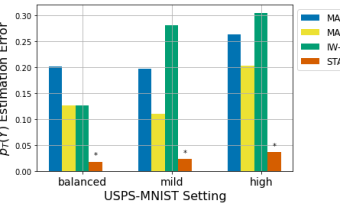
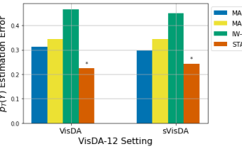
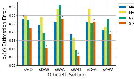
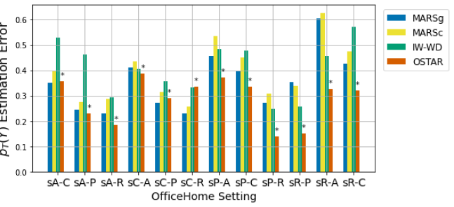
In Table 1, we report, over 10 runs, mean and standard deviations for balanced accuracy, i.e. average recall on each class. This metric is suited for imbalanced problems (Brodersen et al., 2010). For better visibility, results are aggregated over all imbalance settings of a dataset (line “subsampled“). In the Appendix, full results are reported in Table 3 along the $\ell_{1}$ target proportion estimation error for GeTarS baselines and OSTAR+IM in Figure 4. First, we note that low estimation error of $\bm{p}_{T}^{Y}$ is correlated to high accuracy for all models and that DI-Oracle upper-bounds domain-invariant approaches. This shows the importance of correctly estimating $\bm{p}_{T}^{Y}$. Second, we note that OSTAR improves Source (column 2) and is competitive w.r.t. IW-WD (column 9) on VisDA, Office31 and OfficeHome and MARSg (column 7) on Digits although it keeps target representations fixed unlike these two methods. OSTAR+IM (column 11) is less prone to initial target discriminativity and clearly outperforms or equals the baselines on both balanced accuracy and proportion estimation. It even improves DI-Oracle (column 12) for balanced accuracy despite not using true class-ratios. This (i) shows the benefits of not constraining domain-invariance which may degrade target discriminativity especially under label estimation errors; (ii) validates our theoretical results which show that OSTAR controls the target risk and recovers target proportions. We visualize how OSTAR aligns source and target representations in Appendix Figure 3.

Table 1: Balanced accuracy ($\uparrow$) over 10 runs. The best performing model is indicated in bold. Results are aggregated over all imbalance scenarios and adaptation problems within a same dataset.

Setting	Source	DANN	${WD}_{\beta=0}$	${WD}_{\beta=1}$	${WD}_{\beta=2}$	MARSg	MARSc	IW-WD	OSTAR	OSTAR+IM	DI-Oracle
Digits
balanced	$74.98\pm 3.8$	$90.81\pm 1.3$	$92.63\pm 1.0$	$82.80\pm 4.7$	$76.07\pm 7.1$	$92.18\pm 2.2$	$94.91\pm 1.4$	$95.89\pm 0.5$	$91.66\pm 0.9$	$\mathbf{97.51\pm 0.3}$	$96.90\pm 0.2$
subsampled	$75.05\pm 3.1$	$89.91\pm 1.5$	$89.45\pm 1.0$	$81.56\pm 4.8$	$77.77\pm 6.5$	$91.87\pm 2.0$	$93.75\pm 1.4$	$93.22\pm 1.1$	$88.39\pm 1.5$	$\mathbf{96.69\pm 0.7}$	$96.43\pm 0.3$
VisDA12
original	$48.63\pm 1.0$	$53.72\pm 0.9$	$57.40\pm 1.1$	$47.56\pm 0.8$	$36.21\pm 1.8$	$55.62\pm 1.6$	$55.33\pm 0.8$	$51.88\pm 1.6$	$50.37\pm 0.6$	$\mathbf{59.24\pm 0.5}$	$57.61\pm 0.3$
subsampled	$42.46\pm 1.4$	$47.57\pm 0.9$	$47.32\pm 1.4$	$41.48\pm 1.6$	$31.83\pm 3.0$	$55.00\pm 1.9$	$51.86\pm 2.0$	$50.65\pm 1.5$	$49.05\pm 0.9$	$\mathbf{58.84\pm 1.0}$	$55.77\pm 1.1$
Office31
subsampled	$74.50\pm 0.5$	$76.13\pm 0.3$	$76.24\pm 0.3$	$74.23\pm 0.5$	$72.40\pm 1.8$	$80.20\pm 0.4$	$80.00\pm 0.5$	$77.28\pm 0.4$	$76.19\pm 0.8$	$\mathbf{82.61\pm 0.4}$	$81.07\pm 0.3$
OfficeHome
subsampled	$50.56\pm 2.8$	$50.87\pm 1.05$	$53.47\pm 0.7$	$52.24\pm 1.1$	$49.48\pm 1.3$	$56.60\pm 0.4$	$56.22\pm 0.6$	$54.87\pm 0.4$	$54.64\pm 0.7$	$\mathbf{59.51\pm 0.4}$	$57.97\pm 0.3$

Ablation studies

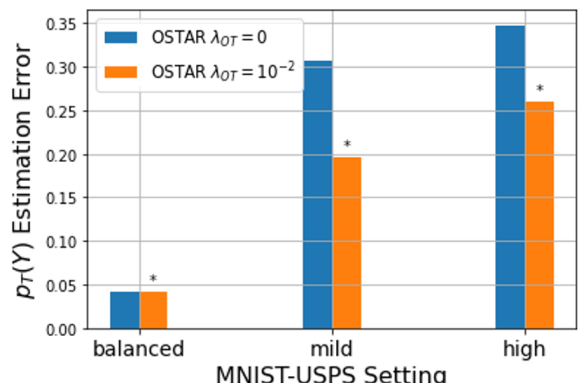
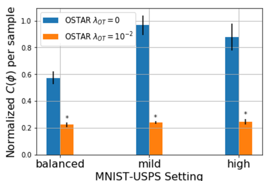
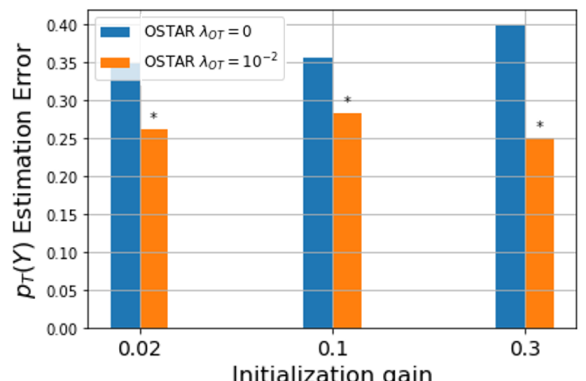
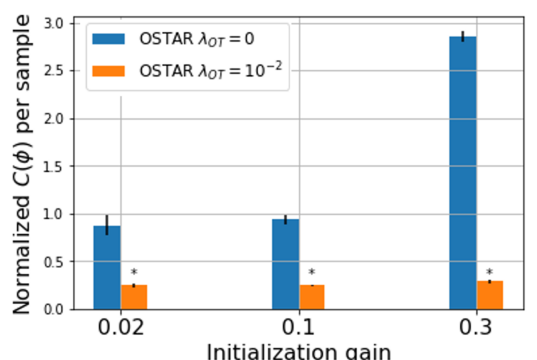
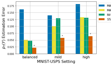
We perform two studies. We first measure the role of IM in our model. In Appendix Table 4, we show the contribution of (SS) (column 3) and (SSg) (column 4) to (CAL) (column 2). We also evaluate the effect of IM on our baselines in Appendix Table 5, even if this is not part of their original work. IM improves performance on VisDA and Office and degrades it on Digits. The performance remains below the ones of OSTAR+IM. Finally, we evaluate the impact of IM on our upper-bound in (2) in Appendix Table 6. We assume that target conditionals are known to compute term LABEL:term_L. We observe that term LABEL:term_C, related to target discriminativity, and the alignment terms LABEL:term_A and LABEL:term_L are reduced. This explains the improvements due to IM and shows empirically that IM helps better optimize the three functions $\phi,g,f_{N}$ in our upper-bound. The second study in Table 2 measures the effect of the OT transport cost in our objective (CAL). Proposition 1 showed that OT guarantees recovering target proportions and matching conditionals. We consider MNIST$\rightarrow$USPS under various shifts (Line 1) and initialization gains i.e. the standard deviation of the weights of the NN (Line 2). On line 1, we note that $\lambda_{OT}\neq 0$ in problem (CAL) improves balanced accuracy (left) and $\ell_{1}$ estimation error (middle) over $\lambda_{OT}=0$ over all shifts, especially high ones. This improvement is correlated with lower mean and standard deviation of the normalized transport cost per sample (right). We observe the same trends when changing initialization gains in Line 2. This confirms our theoretical results and shows the advantages of OT regularization biases for performance and stability. In Appendix Table 7, we test additional values of $\lambda_{OT}$ and see that OSTAR recovers the Source model under high $\lambda_{OT}$. Indeed, the latter constrains $\phi\approx\mathrm{Id}$.

Table 2: Effect of OT on balanced accuracy $\uparrow$ (left), $\ell_{1}$ estimation error $\downarrow$ (middle) and normalized transport cost $\mathcal{L}^{g}_{OT}/n$ $\downarrow$ (right) for MNIST$\rightarrow$USPS. The best model for accuracy is in bold with a “$\star$“. We consider varying shifts (Line 1) and initialization gains (stdev of the NN’s weights) (Line2)

MNIST$\rightarrow$USPS - initialization gain 0.02 Shift $\lambda_{OT}=0$ $\lambda_{OT}=10^{-2}$ balanced $\mathbf{94.92\pm 0.6}$ $\mathbf{95.12\pm 0.6}$ mild $88.28\pm 1.5$ $\mathbf{91.77\pm 1.2}$ high $85.24\pm 1.6$ $\mathbf{88.55\pm 1.1}$

(c)

MNIST$\rightarrow$USPS - high imbalance Init Gain $\lambda_{OT}=0$ $\lambda_{OT}=10^{-2}$ $0.02$ $85.24\pm 1.6$ $\mathbf{88.55\pm 1.1}$ $0.1$ $84.62\pm 2.3$ $\mathbf{88.41\pm 1.3}$ $0.3$ $83.11\pm 2.4$ $\mathbf{89.41\pm 1.6}$

(d)

6 Related Work

UDA

Existing approaches train a classifier using source labels while handling distribution shifts. We review two main approaches: the first learns invariant representations and the second learns a map between fixed samples from source and target domains. While domain-invariant approaches are SOTA, mapping-based approaches avoid structure issues posed by the invariance constraint which may degrade target discriminativity (Liu et al., 2019; Chen et al., 2019). For CovS, domain-invariant methods directly match marginal distributions in latent space (Ganin et al., 2016; Shen et al., 2018; Long et al., 2015), while mapping-based approaches learn a mapping in input space (Courty et al., 2017b; Hoffman et al., 2018). For TarS and GeTarS, label shift requires estimating $\bm{p}_{T}^{Y}$ to reweight source samples by estimated class-ratios (Zhao et al., 2019). An alternative is to use a fixed weight (Wu et al., 2019). When conditionals are unchanged i.e. TarS, $\bm{p}_{T}^{Y}$ can be recovered without needs for alignment (Lipton et al., 2018; Redko et al., 2019). Under GeTarS, there is the additional difficulty of matching conditionals. The SOTA methods for GeTarS are domain-invariant with sample reweighting (Rakotomamonjy et al., 2021; Combes et al., 2020; Gong et al., 2016). An earlier mapping-based approach was proposed in Zhang et al. (2013) to align conditionals, also under reweighting. Yet, it is not flexible, operates on high dimensional input spaces and does not scale up to large label spaces as it considers a linear map for each pair of conditionals. Estimators used in GeTarS are confusion-based in Combes et al. (2020); Shui et al. (2021); derived from optimal assignment in Rakotomamonjy et al. (2021) or from the minimization of a reweighted MMD between marginals in Zhang et al. (2013); Gong et al. (2016). OSTAR is a new mapping-based approach for GeTarS with improvements over these approaches as detailed in this paper. The improvements are both practical (flexibility, scalability, stability) and theoretical. CTC (Gong et al., 2016) also operates on representations, yet OSTAR simplifies learning by clearly separating alignment and encoding operations, intertwined in CTC as both encoder and maps are trained to align.

OT for UDA

A standard approach is to compute a transport plan between empirical distributions with linear programming (LP). LP is used in CovS to align joint distributions (Courty et al., 2017a; Damodaran et al., 2018) or to compute a barycentric mapping in input space (Courty et al., 2017b); and in TarS to estimate target proportions through minimization of a reweighted Wasserstein distance between marginals (Redko et al., 2019). An alternative to LP is to learn invariant representation by minimizing a dual Wasserstein-1 distance with adversarial training as Shen et al. (2018) in CovS or, more recently, Rakotomamonjy et al. (2021); Shui et al. (2021) for GeTarS. Rakotomamonjy et al. (2021) formulates two separate OT problems for class-ratio estimation and conditional alignment and Shui et al. (2021) is the OT extension of Combes et al. (2020) to multi-source UDA. OSTAR is the first OT GeTarS approach that does not learn invariant representations. It has several benefits: (i) representation are kept separate, thus target discriminativity is not deteriorated, (ii) a single OT problem is solved unlike Rakotomamonjy et al. (2021), (iii) the OT map is implemented with a NN which generalizes beyond training samples and scales up with the number of samples unlike barycentric OT maps; (iv) it improves efficiency of matching by encoding samples, thereby improving discriminativity and reducing dimensionality, unlike Courty et al. (2017b).

7 Conclusion

We introduced OSTAR, a new general approach to align pretrained representations under GeTarS, which does not constrain representation invariance. OSTAR learns a flexible and scalable map between conditional distributions in the latent space. This map, implemented as a ResNet, solves an OT matching problem with native regularization biases. Our approach provides strong generalization guarantees under mild assumptions as it explicitly minimizes a new upper-bound to the target risk. Experimentally, it challenges recent invariant GeTarS methods on several UDA benchmarks.

Acknowledgement

We acknowledge financial support from DL4CLIM ANR-19-CHIA- 0018-01, RAIMO ANR-20-CHIA-0021-01, OATMIL ANR-17-CE23-0012 and LEAUDS ANR-18-CE23-0020 Projects of the French National Research Agency (ANR).

Reproducibility Statement

We provide explanations of our assumptions in Section 2.3 and provide our proofs in Appendix E. The datasets used in our experiments are public benchmarks and we provide a complete description of the data processing steps and NN architectures in Appendix G. Our source code is available at https://github.com/mkirchmeyer/ostar.

Appendix A Additional visualisation

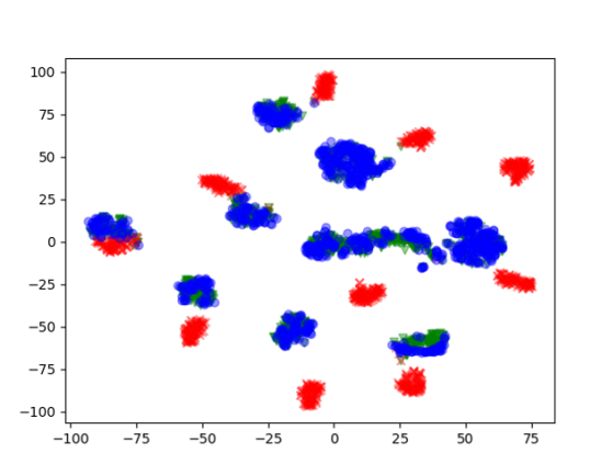
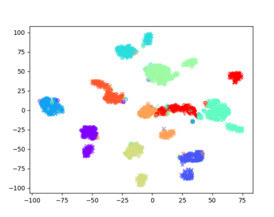
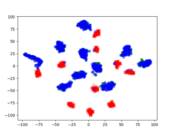
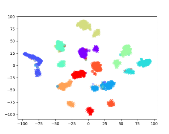
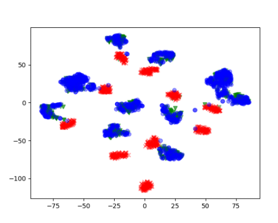
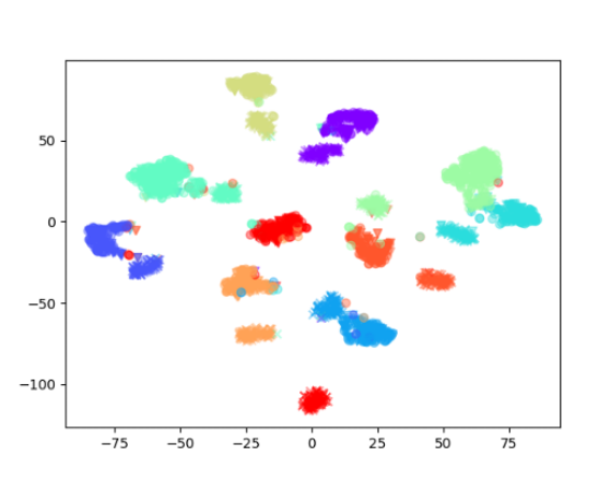
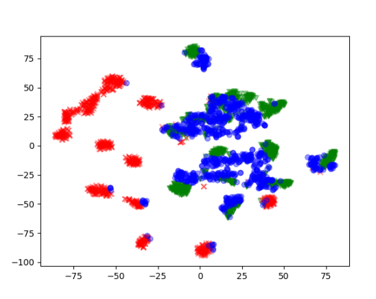
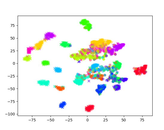
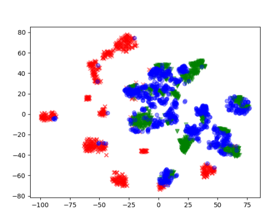
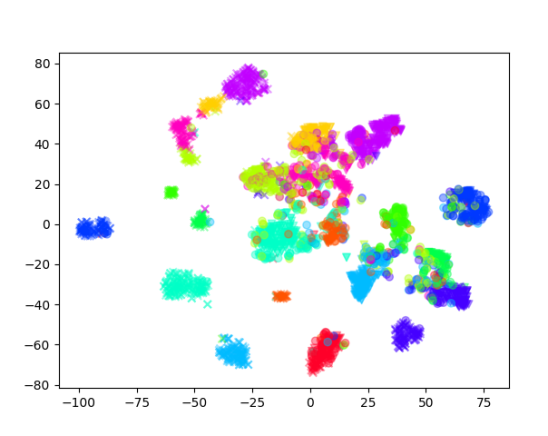
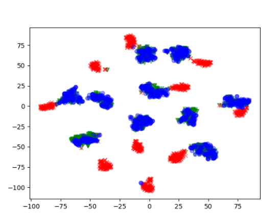
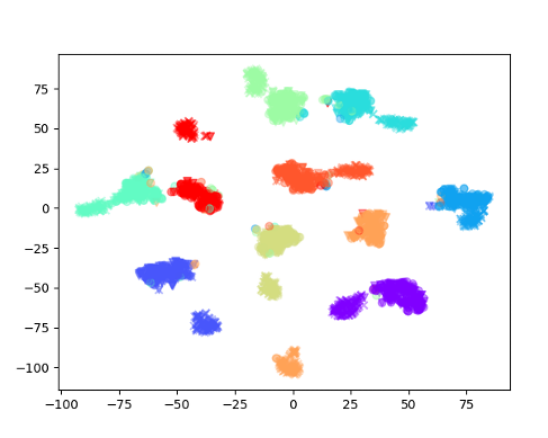
We visualize how OSTAR maps source representations onto target ones under GeTarS. We note that OSTAR (i) maps source conditionals to target ones (blue and green points are matched c.f. left), (ii) matches conditionals of the same class (”v” and ”o” of the same colour are matched c.f. right).

(a)

(b)

(c)

(a)

(b)

(c)

Figure 3: t-SNE feature visualizations for OSTAR on various datasets and label imbalance. Crosses ”x” denote source samples, circles ”o” target samples and triangles ”v” transported source samples. On the left, source samples are red, target samples blue and transported source samples green. On the right, samples from the same class have the same colour regardless of domain.

Appendix B Additional results

We report our full results below. Aggregated results for balanced accuracy over a dataset and imbalance scenarios are reported in Table 1. Prefix ”s” refers to subsampled datasets defined in Table 8.

Table 3: Balanced accuracy ($\uparrow$) over 10 runs. The best performing model is indicated in bold.

Setting	Source	DANN	${WD}_{\beta=0}$	${WD}_{\beta=1}$	${WD}_{\beta=2}$	MARSg	MARSc	IW-WD	OSTAR+IM	DI-Oracle
Digits - MNIST$\rightarrow$USPS
balanced	$86.94\pm 1.1$	$93.97\pm 0.9$	$94.42\pm 0.6$	$82.05\pm 6.3$	$75.14\pm 6.7$	$94.19\pm 1.8$	$\mathbf{96.44\pm 0.3}$	$\mathbf{96.10\pm 0.3}$	$\mathbf{96.91\pm 0.3}$	$96.95\pm 0.2$
mild	$87.10\pm 2.0$	$93.23\pm 1.2$	$91.52\pm 0.6$	$84.07\pm 5.0$	$78.29\pm 7.2$	$94.78\pm 1.0$	$95.18\pm 0.9$	$94.72\pm 0.4$	$\mathbf{96.18\pm 1.0}$	$97.22\pm 0.2$
high	$86.23\pm 2.8$	$93.03\pm 1.0$	$91.14\pm 0.7$	$85.15\pm 2.9$	$78.90\pm 3.8$	$94.50\pm 1.3$	$95.07\pm 0.6$	$94.60\pm 0.8$	$\mathbf{96.06\pm 0.6}$	$96.87\pm 0.4$
Digits - USPS$\rightarrow$MNIST
balanced	$63.01\pm 6.5$	$87.64\pm 1.7$	$90.84\pm 1.3$	$83.54\pm 3.0$	$77.00\pm 7.6$	$90.16\pm 2.5$	$93.37\pm 2.5$	$95.68\pm 0.6$	$\mathbf{98.11\pm 0.2}$	$96.84\pm 0.2$
mild	$62.81\pm 2.3$	$87.00\pm 2.1$	$88.07\pm 1.2$	$77.83\pm 5.4$	$79.41\pm 7.4$	$89.93\pm 2.4$	$93.20\pm 2.8$	$92.73\pm 1.5$	$\mathbf{97.44\pm 0.5}$	$95.75\pm 0.3$
high	$64.04\pm 5.4$	$86.37\pm 1.4$	$87.04\pm 1.4$	$79.17\pm 6.0$	$74.47\pm 7.4$	$88.24\pm 3.3$	$91.54\pm 0.9$	$90.81\pm 1.5$	$\mathbf{97.08\pm 0.6}$	$95.87\pm 0.3$
VisDA12
VisDA	$48.63\pm 1.0$	$53.72\pm 0.9$	$57.40\pm 1.1$	$47.56\pm 0.8$	$36.21\pm 1.8$	$55.62\pm 1.6$	$55.33\pm 0.8$	$51.88\pm 1.6$	$\mathbf{59.24\pm 0.5}$	$57.61\pm 0.3$
sVisDA	$42.46\pm 1.4$	$47.57\pm 0.9$	$47.32\pm 1.4$	$41.48\pm 1.6$	$31.83\pm 3.0$	$55.00\pm 1.9$	$51.86\pm 2.0$	$50.65\pm 1.5$	$\mathbf{58.84\pm 1.0}$	$55.77\pm 1.1$
Office31
sA-D	$80.71\pm 0.5$	$82.39\pm 0.4$	$81.76\pm 0.4$	$75.98\pm 1.2$	$68.64\pm 2.4$	$\mathbf{84.54\pm 1.0}$	$\mathbf{84.10\pm 0.8}$	$81.83\pm 0.5$	$\mathbf{84.17\pm 0.7}$	$87.74\pm 0.6$
sD-W	$89.08\pm 0.4$	$88.70\pm 0.2$	$88.98\pm 0.2$	$88.53\pm 0.2$	$88.97\pm 0.1$	$91.03\pm 0.4$	$90.76\pm 0.4$	$88.17\pm 0.3$	$\mathbf{94.13\pm 0.2}$	$91.31\pm 0.2$
sW-A	$58.91\pm 0.2$	$58.87\pm 0.1$	$59.18\pm 0.2$	$60.70\pm 0.3$	$60.95\pm 0.2$	$63.94\pm 0.1$	$63.80\pm 0.3$	$60.25\pm 0.2$	$\mathbf{69.99\pm 0.1}$	$63.92\pm 0.2$
sW-D	$95.64\pm 0.2$	$97.26\pm 0.3$	$97.13\pm 0.3$	$95.99\pm 0.3$	$95.57\pm 0.5$	$97.96\pm 0.1$	$\mathbf{98.16\pm 0.2}$	$97.53\pm 0.2$	$\mathbf{98.47\pm 0.2}$	$98.35\pm 0.0$
sD-A	$53.41\pm 0.9$	$57.45\pm 0.2$	$57.81\pm 0.2$	$58.24\pm 0.2$	$58.61\pm 0.3$	$62.12\pm 0.2$	$62.13\pm 0.4$	$60.03\pm 0.2$	$\mathbf{65.00\pm 0.5}$	$62.57\pm 0.3$
sA-W	$69.23\pm 0.5$	$72.09\pm 0.5$	$72.60\pm 0.3$	$65.94\pm 0.9$	$61.64\pm 7.2$	$81.60\pm 0.5$	$81.05\pm 0.7$	$75.84\pm 0.7$	$\mathbf{83.91\pm 0.5}$	$82.51\pm 0.5$
OfficeHome
sA-C	$44.44\pm 0.3$	$46.08\pm 0.3$	$41.74\pm 1.7$	$40.90\pm 0.8$	$39.22\pm 1.1$	$47.19\pm 0.3$	$46.94\pm 0.2$	$45.29\pm 0.1$	$\mathbf{48.43\pm 0.2}$	$48.09\pm 0.2$
sA-P	$58.96\pm 0.3$	$59.96\pm 0.2$	$54.67\pm 1.8$	$52.18\pm 2.3$	$46.29\pm 1.4$	$62.17\pm 0.2$	$61.97\pm 0.2$	$59.46\pm 0.3$	$\mathbf{69.52\pm 0.4}$	$63.59\pm 0.2$
sA-R	$67.10\pm 0.2$	$67.42\pm 0.2$	$65.40\pm 0.6$	$62.52\pm 1.7$	$60.51\pm 1.9$	$68.66\pm 0.3$	$68.62\pm 0.3$	$67.76\pm 0.2$	$\mathbf{73.29\pm 0.3}$	$69.85\pm 0.1$
sC-A	$35.54\pm 2.3$	$35.47\pm 1.7$	$37.34\pm 2.0$	$36.81\pm 1.5$	$33.15\pm 2.3$	$\mathbf{46.03\pm 0.2}$	$\mathbf{46.10\pm 0.2}$	$44.18\pm 0.1$	$\mathbf{46.47\pm 0.3}$	$46.94\pm 0.2$
sC-P	$52.48\pm 2.1$	$50.56\pm 0.9$	$53.53\pm 0.1$	$49.96\pm 1.4$	$44.67\pm 1.5$	$59.82\pm 0.1$	$59.82\pm 0.1$	$58.67\pm 0.1$	$\mathbf{63.37\pm 0.1}$	$60.14\pm 0.1$
sC-R	$54.99\pm 1.7$	$54.22\pm 0.8$	$54.69\pm 0.5$	$51.34\pm 2.5$	$45.16\pm 3.5$	$62.69\pm 0.1$	$62.41\pm 0.1$	$60.74\pm 0.2$	$\mathbf{63.12\pm 0.2}$	$62.80\pm 0.2$
sP-A	$38.10\pm 4.5$	$36.36\pm 3.3$	$48.24\pm 0.2$	$47.24\pm 0.3$	$48.20\pm 0.3$	$47.78\pm 0.3$	$46.10\pm 0.9$	$45.68\pm 0.3$	$\mathbf{50.84\pm 0.3}$	$50.11\pm 0.4$
sP-C	$34.16\pm 4.6$	$33.00\pm 1.9$	$39.10\pm 0.2$	$40.36\pm 0.4$	$37.41\pm 0.3$	$42.41\pm 0.3$	$41.92\pm 0.3$	$38.22\pm 0.2$	$\mathbf{44.15\pm 0.3}$	$43.10\pm 0.2$
sP-R	$66.28\pm 3.4$	$59.19\pm 0.8$	$70.01\pm 0.1$	$68.78\pm 0.2$	$66.61\pm 0.3$	$70.00\pm 0.4$	$69.37\pm 0.9$	$69.43\pm 0.4$	$\mathbf{73.95\pm 0.3}$	$71.26\pm 0.4$
sR-P	$66.67\pm 5.4$	$70.97\pm 0.6$	$73.47\pm 0.3$	$72.66\pm 0.7$	$71.76\pm 0.7$	$72.62\pm 0.9$	$72.72\pm 1.1$	$72.90\pm 0.7$	$\mathbf{75.58\pm 0.6}$	$74.17\pm 0.7$
sR-A	$48.59\pm 6.7$	$51.90\pm 1.1$	$\mathbf{56.97\pm 0.3}$	$\mathbf{57.02\pm 0.5}$	$55.38\pm 1.1$	$54.02\pm 0.7$	$53.37\pm 1.3$	$53.44\pm 0.6$	$\mathbf{56.28\pm 0.5}$	$57.68\pm 0.6$
sR-C	$39.36\pm 2.5$	$45.33\pm 0.8$	$46.47\pm 0.4$	$47.11\pm 0.5$	$45.38\pm 1.3$	$45.81\pm 1.2$	$45.30\pm 1.2$	$42.66\pm 1.0$	$\mathbf{49.07\pm 0.9}$	$47.86\pm 0.3$

Figure 4: $\ell_{1}$ estimation error of $\bm{p}_{T}^{Y}$ ($\downarrow$). The best model for balanced accuracy is indicated with ”$\star$”.

Additional ablation studies

We detail the full results for our ablation studies.

Table 4: Semi-supervised learning for OSTAR and balanced accuracy ($\uparrow$). Best results are in bold.

Setting \ Objective (CAL) + (SS) + (SSg) MNIST$\rightarrow$USPS balanced $95.12\pm 0.6$ $96.68\pm 0.1$ $\mathbf{96.91\pm 0.3}$ mild $91.77\pm 1.2$ $95.39\pm 1.4$ $\mathbf{96.18\pm 1.0}$ high $88.55\pm 1.1$ $95.70\pm 0.8$ $\mathbf{96.06\pm 0.6}$ USPS$\rightarrow$MNIST balanced $88.19\pm 1.1$ $97.16\pm 0.3$ $\mathbf{98.11\pm 0.2}$ mild $88.34\pm 1.3$ $96.34\pm 0.2$ $\mathbf{97.44\pm 0.5}$ high $84.87\pm 2.3$ $95.61\pm 0.4$ $\mathbf{97.08\pm 0.6}$ VisDA12 original $50.37\pm 0.6$ $52.54\pm 0.3$ $\mathbf{59.24\pm 0.5}$ subsampled $49.05\pm 0.9$ $53.37\pm 0.6$ $\mathbf{58.84\pm 1.0}$ Office31 sA-D $81.52\pm 0.7$ $83.18\pm 0.2$ $\mathbf{84.17\pm 0.7}$ sD-W $89.94\pm 0.8$ $89.50\pm 0.8$ $\mathbf{94.13\pm 0.2}$ sW-A $59.62\pm 0.6$ $60.06\pm 0.4$ $\mathbf{69.99\pm 0.1}$ sW-D $96.39\pm 0.6$ $97.44\pm 0.2$ $\mathbf{98.47\pm 0.2}$ sD-A $54.38\pm 1.1$ $56.58\pm 0.6$ $\mathbf{65.00\pm 0.5}$ sA-W $75.30\pm 1.0$ $81.32\pm 0.8$ $\mathbf{83.91\pm 0.5}$

Table 5: IM for MARSc, IW-WD and OSTAR on balanced accuracy ($\uparrow$). Best results are in bold.

Setting \ Model	MARSc	MARSc+IM	IW-WD	IW-WD+IM	OSTAR	OSTAR+IM
MNIST$\rightarrow$USPS
balanced	$96.44\pm 0.3$	$\mathbf{97.92\pm 0.2}$	$96.10\pm 0.3$	$\mathbf{97.91\pm 0.1}$	$95.12\pm 0.6$	$96.91\pm 0.3$
mild	$95.18\pm 0.9$	$95.47\pm 1.1$	$94.72\pm 0.4$	$95.74\pm 0.6$	$91.77\pm 1.2$	$\mathbf{96.18\pm 1.0}$
high	$95.07\pm 0.6$	$93.76\pm 0.5$	$94.60\pm 0.8$	$91.73\pm 0.6$	$88.55\pm 1.1$	$\mathbf{96.06\pm 0.6}$
USPS$\rightarrow$MNIST
balanced	$93.37\pm 2.5$	$93.03\pm 1.9$	$95.68\pm 0.6$	$96.17\pm 0.5$	$88.19\pm 1.1$	$\mathbf{98.11\pm 0.2}$
mild	$93.20\pm 2.8$	$94.60\pm 1.7$	$92.73\pm 1.5$	$92.65\pm 1.0$	$88.34\pm 1.3$	$\mathbf{97.44\pm 0.5}$
high	$91.54\pm 0.9$	$90.16\pm 2.0$	$90.81\pm 1.5$	$91.26\pm 1.1$	$84.87\pm 2.3$	$\mathbf{97.08\pm 0.6}$
VisDA12
VisDA	$55.33\pm 0.8$	$57.57\pm 0.8$	$51.88\pm 1.6$	$57.63\pm 0.1$	$50.37\pm 0.6$	$\mathbf{59.24\pm 0.5}$
sVisDA	$51.86\pm 2.0$	$57.06\pm 0.8$	$50.65\pm 1.5$	$57.62\pm 0.7$	$49.05\pm 0.9$	$\mathbf{58.84\pm 1.0}$
Office31
sW-A	$63.80\pm 0.3$	$68.12\pm 0.5$	$60.25\pm 0.2$	$67.42\pm 0.8$	$59.62\pm 0.6$	$\mathbf{69.99\pm 0.1}$
sA-W	$81.05\pm 0.7$	$81.83\pm 1.9$	$75.84\pm 0.7$	$82.34\pm 1.6$	$75.30\pm 1.0$	$\mathbf{83.91\pm 0.5}$
OfficeHome
sR-P	$72.72\pm 1.1$	$\mathbf{75.17\pm 0.6}$	$72.90\pm 0.7$	$74.94\pm 0.6$	$71.77\pm 0.4$	$\mathbf{75.58\pm 0.6}$
sR-A	$53.37\pm 1.3$	$54.20\pm 1.3$	$53.44\pm 0.6$	$54.50\pm 1.1$	$55.15\pm 0.8$	$\mathbf{56.28\pm 0.5}$
sR-C	$45.30\pm 1.2$	$48.17\pm 1.2$	$42.66\pm 1.0$	$47.93\pm 1.7$	$43.02\pm 3.1$	$\mathbf{49.07\pm 0.9}$

Table 6: Best value over training epochs of term LABEL:term_A ($\downarrow$), term LABEL:term_C ($\downarrow$) and term LABEL:term_L ($\downarrow$) without and with IM in OSTAR. Best results are in bold. Terms LABEL:term_A and LABEL:term_L are computed with the primal formulation of OT using the POT package https://pythonot.github.io/.

	Alignment				Discriminativity
	Term (A)		Term (L)		Term (C)
Setting	OSTAR	OSTAR+IM	OSTAR	OSTAR+IM	OSTAR	OSTAR+IM
MNIST$\rightarrow$USPS
balanced	$49.83$	16.56	$1.45$	$\mathbf{0.18}$	$2.19\times 10^{-3}$	$\mathbf{0.918\times 10^{-3}}$
mild	$39.31$	19.13	$10.78$	$\mathbf{0.24}$	$1.65\times 10^{-3}$	$\mathbf{0.931\times 10^{-3}}$
high	$38.60$	21.10	$12.78$	$\mathbf{0.74}$	$1.76\times 10^{-3}$	$\mathbf{0.510\times 10^{-3}}$
USPS$\rightarrow$MNIST
balanced	$235.43$	86.65	$7.08$	$\mathbf{0.52}$	$4.46\times 10^{-3}$	$\mathbf{0.495\times 10^{-3}}$
mild	$188.67$	104.66	$20.99$	$\mathbf{1.05}$	$3.98\times 10^{-3}$	$\mathbf{0.399\times 10^{-3}}$
high	$181.64$	123.83	$21.62$	$\mathbf{0.82}$	$4.51\times 10^{-3}$	$\mathbf{0.616\times 10^{-3}}$

Table 7: Detailed analysis of the impact of $\lambda_{OT}$ on balanced accuracy ($\uparrow$). Best results are in bold.

MNIST$\rightarrow$USPS - initialization gain 0.02
Shift \ $\lambda_{OT}$	$\lambda_{OT}=0$	$\lambda_{OT}=10^{-3}$	$\lambda_{OT}=10^{-2}$	$\lambda_{OT}=10^{-1}$	$\lambda_{OT}=1$	$\lambda_{OT}=10^{4}$	Source
balanced	$94.92\pm 0.6$	$\mathbf{96.02\pm 0.2}$	$95.12\pm 0.6$	$89.76\pm 1.2$	$91.95\pm 1.2$	$87.03\pm 1.8$	$86.02\pm 1.4$
mild	$88.28\pm 1.5$	$88.63\pm 1.3$	$\mathbf{91.77\pm 1.2}$	$90.17\pm 1.7$	$88.51\pm 1.2$	$88.42\pm 1.6$	$89.08\pm 0.5$
high	$85.24\pm 1.6$	$85.38\pm 1.4$	$88.55\pm 1.1$	$\mathbf{89.10\pm 1.2}$	$\mathbf{88.82\pm 1.1}$	$86.94\pm 1.1$	$86.73\pm 1.9$

MNIST$\rightarrow$USPS high imbalance
Gain \ $\lambda_{OT}$	$\lambda_{OT}=0$	$\lambda_{OT}=10^{-3}$	$\lambda_{OT}=10^{-2}$	$\lambda_{OT}=10^{-1}$	$\lambda_{OT}=1$	$\lambda_{OT}=10^{4}$
$0.02$	$85.24\pm 1.6$	$85.38\pm 1.4$	$88.55\pm 1.1$	$\mathbf{89.10\pm 1.2}$	$\mathbf{88.82\pm 1.1}$	$86.94\pm 1.1$
$0.1$	$84.62\pm 2.3$	$85.84\pm 1.1$	$\mathbf{88.41\pm 1.3}$	$\mathbf{88.79\pm 1.2}$	$87.90\pm 1.2$	$87.10\pm 1.0$
$0.3$	$83.11\pm 2.4$	$84.45\pm 1.4$	$89.41\pm 1.6$	$\mathbf{91.00\pm 1.3}$	$89.65\pm 0.7$	$86.23\pm 1.8$

Appendix C Details on Optimal Transport

Background

OT was introduced to find a transportation map minimizing the cost of displacing mass from one configuration to another (Villani, 2008). For a comprehensive introduction, we refer to Peyré & Cuturi (2019). Formally, let $\alpha$ and $\beta$ be absolutely continuous distributions compactly supported in $\mathbb{R}^{d}$ and $c:\mathbb{R}^{d}\times\mathbb{R}^{d}\rightarrow\mathbb{R}$ a cost function. Consider a map $\phi:\mathbb{R}^{d}\rightarrow\mathbb{R}^{d}$ that satisfies $\phi_{\#}\alpha=\beta$, i.e. that pushes $\alpha$ to $\beta$. We remind that for a function $f$, $f_{\#}\rho$ is the push-forward measure $f_{\#}\rho(B)=\rho\left(f^{-1}(B)\right)$, for all measurable set $B$. The total transportation cost depends on the contributions of costs for transporting each point $\mathbf{x}$ to $\phi(\mathbf{x})$ and the Monge OT problem is:

$$\min_{\phi}\mathcal{C}_{\text{monge}}(\phi)=\int_{\mathbb{R}^{d}}c(\mathbf{x},\phi(\mathbf{x}))d\alpha(\mathbf{x})$$ (9)

$$\text{s.t.~{}}\phi_{\#}\alpha=\beta$$

$c(\mathbf{x},\mathbf{y})=\|\mathbf{x}-\mathbf{y}\|_{2}^{p}$ induces the $p$-Wasserstein distance, $\mathcal{W}_{p}(\alpha,\beta)=\min_{\phi_{\#}\alpha=\beta}\mathcal{C}_{\text{monge}}(\phi)^{1/p}$. When $p=1$, $\mathcal{W}_{1}$ can be expressed in the dual form $\mathcal{W}_{1}(\alpha,\beta)=\sup_{\|v\|_{L}\leq 1}\mathbb{E}_{\mathbf{x}\sim\alpha}v(\mathbf{x})-\mathbb{E}_{\mathbf{y}\sim\beta}v(\mathbf{y})$ where $\|v\|_{L}$ is the Lipschitz constant of function $v$.

Relationship between (OT) and the Monge OT problem (9)

(OT) is the extension of (9) to the setting where $\bm{p}_{S}^{Y}\neq\bm{p}_{T}^{Y}$ with $\bm{p}_{T}^{Y}$ unknown. This extension aims at matching conditional distributions regardless of how their mass differ and learns a weighting term $\bm{p}_{N}^{Y}$ for source conditional distributions which addresses label shift settings. When $\bm{p}_{S}^{Y}=\bm{p}_{T}^{Y}$, these two formulations are equivalent under Assumption 1 if we fix $\bm{p}_{N}^{Y}=\bm{p}_{S}^{Y}=\bm{p}_{T}^{Y}$.

Appendix D Discussion

Our four assumptions are required for deriving our theoretical guarantees. All GeTarS papers that propose theoretical guarantees also rely on a set of assumptions, either explicit or implicit. Assumptions 1 and 4 are common to several papers. Assumption 1 is easily met in practice since it could be forced by training a classifier on the source labels. Assumption 4 is said to be met in high dimensions (Redko et al., 2019; Garg et al., 2020). Assumption 3 says that source and target clusters from the same class are globally (there is a sum in the condition) closer one another than clusters from two different classes. This assumption is required to cope with the absence of target labels. Because of the sum, it could be considered as a reasonable hypothesis. It is milder than the hypotheses made in papers offering guarantees similar to ours (Zhang et al., 2013; Gong et al., 2016). Assumption 2 is new to this paper. It states that $\phi$ maps a $j$ source conditional to a unique $k$ target conditional i.e. it guarantees that mass of a source conditional will be entirely transferred to a target conditional and will not be split across several target conditionals. This property is key to show that OSTAR matches source conditionals and their corresponding target conditionals, which is otherwise very difficult to guarantee under GeTarS as both target conditionals and proportions are unknown. This assumption has some restrictions, despite being milder than existing assumptions in GeTarS. First, mass from a source conditional might in practise be split across several target conditionals. In practise, our optimization problem in (CAL) mitigates this problem by learning how to reweight source conditionals to improve alignment. We could additionally apply Laplacian regularization (Ferradans et al., 2013; Carreira-Perpiñán & Wang, 2014) into our OT map $\phi$ but this was not developed in the paper. Second, it assumes a closed-set UDA problem i.e. label domains are the same $\mathcal{Y}_{S}=\mathcal{Y}_{T}$. The setting where $\mathcal{Y}_{S}\neq\mathcal{Y}_{T}$ is more realistic in large scale image pretraining and is another interesting follow-up. Note that OSTAR can address empirically open-set UDA ($\mathcal{Y}_{T}\subset\mathcal{Y}_{S}$) by simply applying L1 regularization on $\bm{p}_{N}^{Y}$ in our objective function (CAL). This forces sparsity and allows ”loosing” mass when mapping a source conditional. It avoids the unwanted negative transfer setting when source clusters, with labels absent on the target, are aligned with target clusters.

Appendix E Proofs

Proposition (1).

For any encoder $g$ which defines $\mathcal{Z}$ satisfying Assumption 1, 2, 3, 4, there is an unique solution $(\phi,\bm{p}_{N}^{Y})$ to (OT) and $\phi_{\#}(p_{S}(Z|Y))=p_{T}(Z|Y)$ and $\bm{p}_{N}^{Y}=\bm{p}_{T}^{Y}$.

Proof.

Fixing $\mathcal{Z}$ satisfying Assumption 1, 3 and 4, we first show that there exists a solution $(\phi,\bm{p}_{N}^{Y})$ to (OT). Following Brenier (1991) as $\mathcal{Z}\subset\mathbb{R}^{d}$, we can find $K$ unique Monge maps $\{\widehat{\phi}^{(k)}\}_{k=1}^{K}$ s.t. $\forall k~{}\widehat{\phi}^{(k)}_{\#}(p_{S}(Z|Y=k))=p_{T}(Z|Y=k)$ with respective transport costs $\mathcal{W}_{1}(p_{S}(Z|Y=k),p_{T}(Z|Y=k))$. Let’s define $\widehat{\phi}$ as $\forall k~{}\widehat{\phi}_{|\mathcal{Z}_{S}^{(k)}}=\widehat{\phi}^{(k)}$ where $\cup_{k=1}^{K}\mathcal{Z}_{S}^{(k)}$ is the partition of $\mathcal{Z}_{S}$ in Assumption 1. $(\widehat{\phi},\bm{p}_{T}^{Y})$ satisfies the equality constraint to (OT), thus we easily deduce existence.

Now, let $(\phi,\bm{p}_{N}^{Y})$ be a solution to (OT), let’s show unicity. We first show that $\phi=\widehat{\phi}$. Under Assumption 2, (OT) is the Monge formulation of the optimal assignment problem between $\{p_{S}(Z|Y=k)\}_{k=1}^{K}$ and $\{p_{T}(Z|Y=k)\}_{k=1}^{K}$ with $\mathbf{C}$ the cost matrix defined by $\mathbf{C}_{ij}=\mathcal{W}_{2}(p_{S}(Z|Y=i),p_{T}(Z|Y=j))$. At the optimum, the transport cost is related to the Wasserstein distance between source conditionals and their corresponding target conditionals i.e. $\mathcal{C}(\phi)=\sum_{k=1}^{K}\mathcal{W}_{2}(p_{S}(Z|Y=k),\phi_{\#}(p_{S}(Z|Y=k)))$. Suppose $\exists(i,j),j\neq i$ s.t. $\phi_{\#}(p_{S}(Z|Y=i))=p_{T}(Z|Y=j)$ and $\phi_{\#}(p_{S}(Z|Y=j))=p_{T}(Z|Y=i)$ and $\forall k\neq i,j,\phi_{\#}(p_{S}(Z|Y=k))=p_{T}(Z|Y=k)$. Assumption 3 implies $\sum_{k=1}^{K}\mathcal{W}_{2}(p_{S}(Z|Y=k),p_{T}(Z|Y=k))\leq\sum_{k\neq i,j}\mathcal{W}_{2}(p_{S}(Z|Y=k),p_{T}(Z|Y=k))+\mathcal{W}_{2}(p_{S}(Z|Y=i),p_{T}(Z|Y=j))+\mathcal{W}_{2}(p_{S}(Z|Y=j),p_{T}(Z|Y=i))$. Thus $C(\widehat{\phi},\mathcal{Z})\leq C(\phi,\mathcal{Z})$ whereas $\phi$, solution to (OT), has minimal transport cost. Thus $\phi=\widehat{\phi}$.

Now let’s show ${\bm{p}_{N}^{Y}}=\bm{p}_{T}^{Y}$ under Assumption 4. We inject $\phi_{\#}(p_{S}(Z|Y))=p_{T}(Z|Y)$ into (OT),

$$\sum_{k=1}^{K}{\bm{p}_{N}^{Y=k}}p_{T}(Z|k)=\sum_{k=1}^{K}\bm{p}_{T}^{Y=k}p_{T}(Z|k)\Leftrightarrow\sum_{k=1}^{K}\left({\bm{p}_{N}^{Y=k}}-\bm{p}_{T}^{Y=k}\right)p_{T}(Z|k)=0\Leftrightarrow{\bm{p}_{N}^{Y}}=\bm{p}_{T}^{Y}$$

∎

Theorem (1).

Given a fixed encoder $g$ defining a latent space $\mathcal{Z}$, two domains $N$ and $T$ satisfying cyclical monotonicity in $\mathcal{Z}$, assuming that we have $\forall k,\bm{p}_{N}^{Y=k}>0$, then $\forall f_{N}\in\mathcal{H}$ where $\mathcal{H}$ is a set of $M$-Lipschitz continuous functions over $\mathcal{Z}$, we have

$$\epsilon_{T}^{g}(f_{N}) \leq\underbrace{\epsilon_{N}^{g}(f_{N})}_{\mathrm{Classification~{}}\ref{term_C}}+\underbrace{\dfrac{2M}{\min_{k=1}^{K}\bm{p}_{N}^{Y=k}}\mathcal{W}_{1}\Big{(}p_{N}(Z),p_{T}(Z)\Big{)}}_{\mathrm{Alignment~{}}\ref{term_A}}$$ (2)

$$+ \underbrace{2M\Big{(}1+\dfrac{1}{\min_{k=1}^{K}\bm{p}_{N}^{Y=k}}\Big{)}\mathcal{W}_{1}\Big{(}\sum_{k=1}^{K}\bm{p}_{N}^{Y=k}p_{T}(Z|Y=k),\sum_{k=1}^{K}\bm{p}_{T}^{Y=k}p_{T}(Z|Y=k)\Big{)}}_{\mathrm{Label~{}}\ref{term_L}}$$

Proof.

We first recall that $\epsilon_{D}^{g}(f_{N})=\mathbb{E}_{(\mathbf{z},y)\in p_{D}(Z,Y)}\mathcal{L}(f_{N}(\mathbf{z}),y)$ where $\mathcal{L}$ is the 0/1 loss. For conciseness, $\forall\mathbf{z}\in\mathcal{Z}$, $\bm{p_{T}}^{\mathbf{z}|Y},\bm{p_{N}}^{\mathbf{z}|Y},\mathcal{L}^{\mathbf{z},k}$ will refer to the vector of $[p_{T}(\mathbf{z}|k)]_{k=1}^{K}$, $[p_{N}(\mathbf{z}|k)]_{k=1}^{K}$, $[\mathcal{L}(f_{N}(\mathbf{z}),k)]_{k=1}^{K}$ respectively. In the following, $\odot$ denotes the element-wise product operator between two vectors of the same size.

$$\forall f_{N},\epsilon_{T}^{g}(f_{N})=\epsilon_{N}^{g}(f_{N})+\epsilon_{T}^{g}(f_{N})-\epsilon_{N}^{g}(f_{N})$$

$$\leq\epsilon_{N}^{g}(f_{N})+\int_{\mathcal{Z}}\sum_{k=1}^{K}\Big{(}p_{T}(\mathbf{z},k)-p_{N}(\mathbf{z},k)\Big{)}\times\mathcal{L}\Big{(}f_{N}(\mathbf{z}),k\Big{)}d\mathbf{z}dy$$

$$\leq\epsilon_{N}^{g}(f_{N})+\int_{\mathcal{Z}}\sum_{k=1}^{K}\Big{[}\bm{p}_{T}^{Y=k}p_{T}(\mathbf{z}|k)-\bm{p}_{N}^{Y=k}p_{N}(\mathbf{z}|k)\Big{]}\times\mathcal{L}\Big{(}f_{N}(\mathbf{z}),k\Big{)}d\mathbf{z}$$

$$\leq\epsilon_{N}^{g}(f_{N})+\int_{\mathcal{Z}}{\bm{p}_{T}^{Y}}^{\intercal}\Big{(}\bm{p_{T}}^{\mathbf{z}|Y}\odot\mathcal{L}^{\mathbf{z},k}\Big{)}-{\bm{p}_{N}^{Y}}^{\intercal}\Big{(}\bm{p_{N}}^{\mathbf{z}|Y}\odot\mathcal{L}^{\mathbf{z},k}\Big{)}d\mathbf{z}$$

$$\leq\epsilon_{N}^{g}(f_{N})+\int_{\mathcal{Z}}{\bm{p}_{T}^{Y}}^{\intercal}\Big{(}\bm{p_{T}}^{\mathbf{z}|Y}\odot\mathcal{L}^{\mathbf{z},k}\Big{)}-{\bm{p}_{N}^{Y}}^{\intercal}\Big{(}\bm{p_{T}}^{\mathbf{z}|Y}\odot\mathcal{L}^{\mathbf{z},k}\Big{)}+{\bm{p}_{N}^{Y}}^{\intercal}\Big{(}\bm{p_{T}}^{\mathbf{z}|Y}\odot\mathcal{L}^{\mathbf{z},k}\Big{)}-{\bm{p}_{N}^{Y}}^{\intercal}\Big{(}\bm{p_{N}}^{\mathbf{z}|Y}\odot\mathcal{L}^{\mathbf{z},k}\Big{)}d\mathbf{z}$$

$$\leq\epsilon_{N}^{g}(f_{N})+\int_{\mathcal{Z}}\Big{(}{\bm{p}_{T}^{Y}}^{\intercal}-{\bm{p}_{N}^{Y}}^{\intercal}\Big{)}\Big{(}\bm{p_{T}}^{\mathbf{z}|Y}\odot\mathcal{L}^{\mathbf{z},k}\Big{)}+{\bm{p}_{N}^{Y}}^{\intercal}\Big{(}(\bm{p_{T}}^{\mathbf{z}|Y}-\bm{p_{N}}^{\mathbf{z}|Y})\odot\mathcal{L}^{\mathbf{z},k}\Big{)}d\mathbf{z}$$

$$\leq\epsilon_{N}^{g}(f_{N})+\int_{\mathcal{Z}}\Big{(}{\bm{p}_{T}^{Y}}^{\intercal}-{\bm{p}_{N}^{Y}}^{\intercal}\Big{)}\Big{(}\bm{p_{T}}^{\mathbf{z}|Y}\odot\mathcal{L}^{\mathbf{z},k}\Big{)}d\mathbf{z}+\int_{\mathcal{Z}}{\bm{p}_{N}^{Y}}^{\intercal}\Big{(}(\bm{p_{T}}^{\mathbf{z}|Y}-\bm{p_{N}}^{\mathbf{z}|Y})\odot\mathcal{L}^{\mathbf{z},k}\Big{)}d\mathbf{z}$$

We now introduce a preliminary result from Shen et al. (2018). $\forall f_{N}\in\mathcal{H}$ $M$-Lipschitz continuous,

$$\epsilon_{N}^{g}(f_{N})-\epsilon_{T}^{g}(f_{N})\leq 2M\cdot\mathcal{W}_{1}(p_{N}^{g}(Z),p_{T}^{g}(Z))$$

Assuming that $h$ is $M$-Lipschitz continuous we apply this result in the following

$$\int_{\mathcal{Z}}\Big{(}{\bm{p}_{T}^{Y}}^{\intercal}-{\bm{p}_{N}^{Y}}^{\intercal}\Big{)}\Big{(}\bm{p_{T}}^{\mathbf{z}|Y}\odot\mathcal{L}^{\mathbf{z},k}\Big{)}d\mathbf{z} =\int_{\mathcal{Z}}\sum_{k=1}^{K}\Big{(}\bm{p}_{T}^{Y=k}-\bm{p}_{N}^{Y=k}\Big{)}p_{T}(\mathbf{z}|k)\times\mathcal{L}\Big{(}f_{N}(\mathbf{z}),k\Big{)}d\mathbf{z}$$

$$=\epsilon_{T}^{g}(f_{N})-\epsilon_{\widetilde{T}}^{g}(f_{N})\quad\text{where~{}}p_{\widetilde{T}}(Z)=\sum_{k=1}^{K}\bm{p}_{N}^{Y=k}p_{T}(Z|k)$$

$$\leq 2M\cdot\mathcal{W}_{1}(p_{\widetilde{T}}(Z),p_{T}(Z))$$

$$\int_{\mathcal{Z}}{\bm{p}_{N}^{Y}}^{\intercal}\Big{(}(\bm{p_{T}}^{\mathbf{z}|Y}-\bm{p_{N}}^{\mathbf{z}|Y})\odot\mathcal{L}^{\mathbf{z},k}\Big{)}d\mathbf{z} =\int_{\mathcal{Z}}\sum_{k=1}^{K}\bm{p}_{N}^{Y=k}\Big{(}p_{T}(\mathbf{z}|k)-p_{N}(\mathbf{z}|k)\Big{)}\times\mathcal{L}\Big{(}f_{N}(\mathbf{z}),k\Big{)}d\mathbf{z}$$

$$\leq\sum_{k=1}^{K}\int_{\mathcal{Z}}\Big{(}p_{T}(\mathbf{z}|k)-p_{N}(\mathbf{z}|k)\Big{)}\times\mathcal{L}\Big{(}f_{N}(\mathbf{z}),k\Big{)}d\mathbf{z}\quad{\forall k~{}\bm{p}_{N}^{Y=k}\leq 1}$$

$$\leq 2M\sum_{k=1}^{K}\mathcal{W}_{1}\Big{(}p_{T}(Z|k),p_{N}(Z|k)\Big{)}$$

Thus, $\forall f_{N}$ $M$-Lipschitz continuous

$$\epsilon_{T}^{g}(f_{N})\leq\epsilon_{N}^{g}(f_{N})+2M\times\sum_{k=1}^{K}\mathcal{W}_{1}\Big{(}p_{T}(Z|k),p_{N}(Z|k)\Big{)}+2M\times\mathcal{W}_{1}\Big{(}p_{\widetilde{T}}(Z),p_{T}(Z)\Big{)}$$

We rewrite the second term to involve directly latent marginals. Proposition 2 in Rakotomamonjy et al. (2021) shows that under cyclical monotonicity, if $\forall k,\bm{p}_{N}^{Y=k}>0$,

$$\mathcal{W}_{1}\Big{(}\sum_{k=1}^{K}\bm{p}_{N}^{Y=k}p_{T}(Z|k),p_{N}(Z)\Big{)}=\sum_{k=1}^{K}\bm{p}_{N}^{Y=k}\mathcal{W}_{1}\Big{(}p_{N}(Z|k),p_{T}(Z|k)\Big{)}$$

This allows to write

$$\min_{k=1}^{K}\bm{p}_{N}^{Y=k} \sum_{k=1}^{K}\mathcal{W}_{1}\Big{(}p_{N}(Z|k),p_{T}(Z|k)\Big{)}\leq\sum_{k=1}^{K}\bm{p}_{N}^{Y=k}\mathcal{W}_{1}\Big{(}p_{N}(Z|k),p_{T}(Z|k)\Big{)}$$

$$=\mathcal{W}_{1}\Big{(}\sum_{k=1}^{K}\bm{p}_{N}^{Y=k}p_{T}(Z|k),p_{N}(Z)\Big{)}=\mathcal{W}_{1}\Big{(}p_{\widetilde{T}}(Z),p_{N}(Z)\Big{)}$$

We then use the triangle inequality for the Wasserstein distance $\mathcal{W}_{1}$

$$\epsilon_{T}^{g}(f_{N}) \leq\epsilon_{N}^{g}(f_{N})+\dfrac{2M}{\min_{k=1}^{K}\bm{p}_{N}^{Y=k}}\mathcal{W}_{1}\Big{(}p_{\widetilde{T}}(Z),p_{N}(Z)\Big{)}+2M\times\mathcal{W}_{1}\Big{(}p_{\widetilde{T}}(Z),p_{T}(Z)\Big{)}$$

$$\leq\epsilon_{N}^{g}(f_{N})+\dfrac{2M}{\min_{k=1}^{K}\bm{p}_{N}^{Y=k}}\mathcal{W}_{1}\Big{(}p_{N}(Z),p_{T}(Z)\Big{)}+2M(1+\dfrac{1}{\min_{k=1}^{K}\bm{p}_{N}^{Y=k}})\mathcal{W}_{1}\Big{(}p_{\widetilde{T}}(Z),p_{T}(Z)\Big{)}$$

∎

Derivation of the reweighted classification loss LABEL:term_C $\epsilon_{N}^{g}(f_{N})$

Let $\mathcal{L}_{ce}$ be the cross-entropy loss. Given a classifier $h$, feature extractor $g$ and domain $N$, the mapping of domain $S$ by $(\phi,\bm{p}_{N}^{Y})$,

$$\epsilon_{N}^{g}(f_{N})=\int_{\mathcal{Z},\mathcal{Y}}p_{N}^{\phi}(\mathbf{z},y)\mathcal{L}_{ce}\Big{(}f_{N}(\mathbf{z}),y\Big{)}d\mathbf{z}dy=\int_{\mathcal{Z},\mathcal{Y}}\bm{p}_{N}^{Y=y}p_{N}^{\phi}(\mathbf{z}|y)\mathcal{L}_{ce}\Big{(}f_{N}(\mathbf{z}),y\Big{)}d\mathbf{z}dy$$

$$=\int_{\mathcal{Z},\mathcal{Y}}\dfrac{\bm{p}_{N}^{Y=y}}{\bm{p}_{S}^{Y=y}}\bm{p}_{S}^{Y=y}p_{N}^{\phi}(\mathbf{z}|y)\mathcal{L}_{ce}\Big{(}f_{N}(\mathbf{z}),y\Big{)}d\mathbf{z}dy=\int_{\mathcal{Z},\mathcal{Y}}\dfrac{\bm{p}_{N}^{Y=y}}{\bm{p}_{S}^{Y=y}}\bm{p}_{S}^{Y=y}\phi_{\#}(p_{S}(\mathbf{z}|y))\mathcal{L}_{ce}\Big{(}f_{N}(\mathbf{z}),y\Big{)}d\mathbf{z}dy$$

Appendix F Pseudo-code and runtime / complexity analysis

We detail in Algorithm 1 our pseudo-code and in Algorithm 2 how we minimize (CAL) with respect to $(\phi,f_{N})$ using the dual form of Wasserstein-1 distance (6). Our method is based on a standard backpropagation strategy with gradient descent and uses gradient penalty (Gulrajani et al., 2017).

Algorithm 1 Training and inference procedure for OSTAR

Training:

$\widehat{S}=\{\mathbf{x_{S}^{(i)}},y_{S}^{(i)}\}_{i=1}^{n}$, $\widehat{T}=\{\mathbf{x_{T}^{(i)}}\}_{i=1}^{m}$, $\mathcal{Z}_{\widehat{N}}=\{\phi\circ g(\mathbf{x_{S}^{(i)}}),y_{S}^{(i)}\}_{i=1}^{n}$, $\mathcal{Z}_{\widehat{T}}=\{g(\mathbf{x_{T}^{(i)}})\}_{i=1}^{m}$

$f_{S},f_{N}\in\mathcal{H}$ classifiers; $g$ feature extractor; $\phi$ latent domain-mapping, $v$ critic.

$N_{e}$: number of epochs, $N_{u}$: epoch to update $\bm{p}_{N}^{Y}$, $N_{g}$: epoch to update $g$

1:Train $f_{S},g$ on $\widehat{S}$ to minimize source classification loss $\triangleright$ (3)

2:Initialize $\bm{p}_{N}^{Y}=\dfrac{1}{K}\mathbf{1}_{K}$

3:for $n_{epoch}\leq N_{e}$ do

4:     if $n_{epoch}\mod N_{u}=0$ then

5:         Compute $\bm{p}_{N}^{Y}$ with estimator in Lipton et al. (2018) on ($\mathcal{Z}_{\widehat{N}}$, $\mathcal{Z}_{\widehat{T}}$) $\triangleright$ (CAL) w.r.t. $\bm{p}_{N}^{Y}$

6:         Average $\bm{p}_{N}^{Y}$ with cumulative moving average      

7:     if $n_{epoch}\leq N_{g}$ then Train $\phi,v,f_{N}$ with $(\widehat{S},\widehat{T})$ $\triangleright$ (CAL) + (SS) w.r.t. $\phi,f_{N}$

8:     else Train $\phi,v,f_{N},g$ with $(\widehat{S},\widehat{T})$ $\triangleright$ (CAL) + (SSg) w.r.t. $\phi,f_{N}$      

Inference: Score $\mathbf{x_{T}}$ with $f_{N}\circ g(\mathbf{x_{T}})$

Algorithm 2 Minimize (CAL) w.r.t. $(\phi,f_{N})$

$\widehat{S}=\{\mathbf{x_{S}^{(i)}},y_{S}^{(i)}\}_{i=1}^{n}$, $\widehat{T}=\{\mathbf{x_{T}^{(i)}}\}_{i=1}^{m}$, $g$ feature extractor, $\phi$ domain-mapping, $v$ critic, $f_{N}$ classifier.

Parameters of $\phi,v,f_{N}$: $\theta_{\phi},\theta_{v},\theta_{f_{N}}$ and learning rates $\alpha_{\phi},\alpha_{v},\alpha_{f_{N}}$.

$N_{iter}$: batches per epoch, $N_{b}$: batch size, $N_{v}$: critic iterations

1:for $n_{iter}<N_{iter}$ do

2:     Sample minibatches $\mathbf{x_{S}^{B}},y_{S}^{B}=\{\mathbf{x_{S}^{(i)}},y_{S}^{(i)}\}_{i=1}^{N_{b}}$, $\mathbf{x_{T}^{B}}=\{\mathbf{z_{T}^{(i)}}\}_{i=1}^{N_{b}}$ from $\widehat{S},\widehat{T}$

3:     Compute $\mathbf{z_{S}^{B}}=g(\mathbf{x_{S}^{B}})$, $\mathbf{z_{N}^{B}}=\phi\circ g(\mathbf{x_{S}^{B}})$ and $\mathbf{z_{T}^{B}}=g(\mathbf{x_{T}^{B}})$

4:     Compute class ratios: $\mathbf{w}_{Y}=\bm{p}_{N}^{Y}/\bm{p}_{S}^{Y}$

5:     for $n_{v}<N_{v}$ do

6:         Sample random points ${\mathbf{z^{B}}}^{\prime}$ from the lines between $(\mathbf{z_{N}^{B}},\mathbf{z_{T}^{B}})$ pairs

7:         Compute gradient penalty $\mathcal{L}_{grad}$ with $\mathbf{z_{N}^{B}},\mathbf{z_{T}^{B}},{\mathbf{z^{B}}}^{\prime}$ (Gulrajani et al., 2017)

8:         Compute $\mathcal{L}_{wd}^{g}=\sum_{i=1}^{N_{b}}\mathbf{w}_{y_{S}^{(i)}}v(\mathbf{z_{N}^{(i)}})-\dfrac{1}{N_{b}}\sum_{i=1}^{N_{b}}v(\mathbf{z_{T}^{(i)}})$ (6)

9:         $\theta_{v}\leftarrow\theta_{v}-\alpha_{v}\nabla_{\theta_{v}}\Big{[}\mathcal{L}_{wd}^{g}-\mathcal{L}_{grad}\Big{]}$      

10:     Compute $\mathcal{L}_{OT}^{g}=\sum_{k=1}^{K}\dfrac{1}{\#\{y_{S}^{(i)}=k\}_{i\in\llbracket 1,N_{b}\rrbracket}}\sum_{y_{S}^{(i)}=k,~{}i\in\llbracket 1,N_{b}\rrbracket}\|\phi(\mathbf{z_{S}^{(i)}})-\mathbf{z_{S}^{(i)}}\|_{2}^{2}$

11:     $\theta_{\phi}\leftarrow\theta_{\phi}-\alpha_{\phi}\nabla_{\theta_{\phi}}\Big{[}\mathcal{L}_{wd}^{g}+\mathcal{L}_{OT}^{g}\Big{]}$

12:     Compute $\mathcal{L}_{c}^{g}(f_{N},N)=\dfrac{1}{N_{b}}\sum_{i=1}^{N_{b}}\mathbf{w}_{y_{S}^{(i)}}\mathcal{L}_{ce}(f_{N}\circ\phi\circ g(\mathbf{x_{S}^{(i)}}),y_{S}^{(i)})$

13:     $\theta_{f_{N}}\leftarrow\theta_{f_{N}}-\alpha_{f_{N}}\nabla_{\theta_{f_{N}}}\mathcal{L}_{c}^{g}(f_{N},N)$

Complexity / Runtime analysis

In practise on USPS $\rightarrow$ MNIST, the runtimes in seconds on a NVIDIA Tesla V100 GPU machine are the following: DANN: 22.75s, $\text{WD}_{\beta=0}$: 59.25s, MARSc: 72.87s, MARSg: 2769.06s, IW-WD: 74.17s, OSTAR+IM: 89.72s. We observe that (i) computing Wasserstein distance ($\text{WD}_{\beta=0}$) is slower than computing $\mathcal{H}$-divergence (DANN), (ii) runtimes for domain-invariant GeTarS baselines are slightly higher than for $\text{WD}_{\beta=0}$ as proportions are additionally estimated, (iii) domain-invariant GeTarS baselines have similar runtimes apart from MARSg which uses GMM, (iv) our model, OSTAR+IM, has slightly higher runtime than GeTarS baselines other than MARSg. We now provide some further analysis on computational cost and memory in OSTAR. We denote $K$ the number of classes, $d$ the dimension of latent representations, $n$ and $m$ the number of source and target samples.

• Memory: Proportion estimation is based on the method in Lipton et al. (2018) and requires storing the confusion matrix $\hat{\mathbf{C}}$ and predictions $\hat{\bm{p}}_{T}^{Y}$ with a memory cost of $O(K^{2})$. Encoding is performed by a deep NN $g$ into $\mathbb{R}^{d}$ and classification by a shallow classifier from $\mathbb{R}^{d}$ to $\mathbb{R}^{K}$. Alignment is performed with a ResNet $\phi:\mathbb{R}^{d}\rightarrow\mathbb{R}^{d}$ in the latent space which has an order magnitude less parameters than $g$. Globally, memory consumption is mostly defined by the number of parameters in the encoder $g$.

• Computational cost comes from: (i) proportion estimation, which depends on $K,n+m$ and is solved once every 5 epochs with small runtime; (ii) alignment between source and target representations, which depends on $d,n+m$ and $N_{v}$ (the number of critic iterations). This step updates less parameters than domain-invariant methods which align with $g$ instead of $\phi$; this may lead to speedups for large encoders. The transport cost $\mathcal{L}^{g}_{OT}$ depends on $n,d$ and adds small additional runtime; (iii) classification with $f_{N}$ using labelled source samples, which depends on $d,K,n$. In a second stage, we improve target discriminativity by updating the encoder $g$ with semi-supervised learning; this depends on $d,K,n+m$.

Appendix G Experimental setup

Datasets

We consider the following UDA problems:

• Digits is a synthetic binary adaptation problem. We consider adaptation between MNIST and USPS datasets. We consider a subsampled version of the original datasets with the following number of samples per domain: 10000-2609 for MNIST$\rightarrow$USPS, 5700-20000 for USPS$\rightarrow$MNIST. The feature extractor is learned from scratch.

• VisDA12 is a 12-class adaptation problem between simulated and real images. We consider a subsampled version of the original problem using 9600 samples per domain and use pre-trained ImageNet ResNet-50 features http://csr.bu.edu/ftp/visda17/clf/.

• Office31 is an object categorization problem with 31 classes. We do not sample the original dataset. There are 3 domains: Amazon (A), DSLR (D) and WebCam (W) and we consider all pairwise source-target domains. We use pre-trained ImageNet ResNet-50 features https://github.com/jindongwang/transferlearning/blob/master/data/dataset.md.

• OfficeHome is another object categorization problem with 65 classes. We do not sample the original dataset. There are 4 domains: Art (A), Product (P), Clipart (C), Realworld (R) and we consider all pairwise source-target domains. We use pre-trained ImageNet ResNet-50 features https://github.com/jindongwang/transferlearning/blob/master/data/dataset.md.

Imbalance settings

We consider different class-ratios between domains to simulate label-shift and denote with a ”s” prefix, the subsampled datasets. For Digits, we explicitly provide the class-ratios as Rakotomamonjy et al. (2021) (e.g. for high imbalance, class 2 accounts for the 7% of target samples while class 4 accounts for 22% of target samples). For Visda12, Office31 and OfficeHome, subsampled datasets only consider a small percentage of source samples for the first half classes as Combes et al. (2020) (e.g. Office31 considers 30% of source samples in classes below 15 and uses all source samples from other classes and all target samples).

Table 8: Label imbalance settings

Dataset	Configuration	$\bm{p}_{S}^{Y}$	$\bm{p}_{T}^{Y}$
Digits	balanced	{$\frac{1}{10},\cdots,\frac{1}{10}$}	{$\frac{1}{10},\cdots,\frac{1}{10}$}
	subsampled mild	{$\frac{1}{10},\cdots,\frac{1}{10}$}	$\{0,1,2,3,6\}=0.06,\{4,5\}=0.2,\{7,8,9\}=0.1$
	subsampled high	{$\frac{1}{10},\cdots,\frac{1}{10}$}	$\{0,1,2,3,6,7,8,9\}=0.07,\{4,5\}=0.22$
VisDA12	original	$\{0-11\}:100\%$	$\{0-11\}:100\%$
	subsampled	$\{0-5\}:30\%$ $\{5-11\}:100\%$	$\{0-11\}:100\%$
Office31	subsampled	$\{0-15\}:30\%$ $\{15-31\}:100\%$	$\{0-31\}:100\%$
OfficeHome	subsampled	$\{0-32\}:30\%$ $\{33-64\}:100\%$	$\{0-64\}:100\%$

Hyperparameters

Domain-invariant methods weight alignment over classification; we tuned the corresponding hyperparameter for $\texttt{WD}_{\beta=0}$ in the range $[10^{-4},10^{-2}]$ and used the one that achieves the best performance on other models. We also tuned $\lambda_{OT}$ in problem (CAL) and fixed it to $10^{-2}$ on Digits and $10^{-5}$ on VisDA12, Office31 and OfficeHome. Batch size is $N_{b}=200$ and all models are trained using Adam with learning rate tuned in the range $[10^{-4},10^{-3}]$. We initialize NN for classifiers and feature extractors with a normal prior with zero mean and gain 0.02 and $\phi$ with orthogonal initialization with gain 0.02.

Training procedure

We fix $N_{e}$ the number of epochs to 50 on Digits, 150 on VisDA12 and 100 on Office31, OfficeHome; OSTAR requires smaller $N_{e}$ to converge. Critic iterations are fixed to $N_{v}=5$ which worked best for all baseline models; for OSTAR higher values performed better. For all models, we initialize $f_{S},g$ for 10 epochs with (3). Then, we perform alignment either through domain-invariance or with a domain-mapping until we reach the total number of epochs. GeTarS models IW-WD, MARSc, MARSg, OSTAR perform reweighting with estimates refreshed every $N_{u}=2$ epochs in the first 10 alignment epochs, every $N_{u}=5$ epochs after. OSTAR minimizes (CAL) + (SS) for 10 epochs on Digits, Office31, OfficeHome and 5 epochs on VisDA12, then minimizes (CAL) + (SSg) for remaining epochs.

Architectures

For Digits, our feature extractor $g$ is composed of three convolutional layers with respectively 64, 64, 128 filters of size $5\times 5$ interleaved with batch norm, max-pooling and ReLU. Our classifiers ($f_{S},f_{N}$) are three-layered fully-connected networks with 100 units interleaved with batch norm, ReLU. Our discriminators are three-layered NN with 100 units and ReLU activation. For VisDA12 and Office31, OfficeHome, we consider pre-trained 2048 features obtained from a ResNet-50 followed by 2 fully-connected networks with ReLU and 100 units for VisDA12, 256 units for Office31, OfficeHome. Discriminators are 2-layer fully-connected networks with respectively 100/1 units on VisDA12, 256/1 units on Office31, OfficeHome interleaved with ReLU. Classifiers are 2-layer fully-connected networks with 100/$K$ units on VisDA12, single layer fully-connected network with $K$ units on Office31, OfficeHome. $\phi$ is a ResNet with $10$ blocks of two fully-connected layers with ReLU and batch-norm.

Implementation of target proportion estimators

OSTAR and IW-WD use the confusion based estimator in Lipton et al. (2018) and solve a convex optimization problem ((4) in Combes et al. (2020) and CAL w.r.t $\bm{p}_{N}^{Y}$ for OSTAR) which has an unique solution if the soft confusion matrix $\mathbf{C}$ is of full rank. We implement the same optimization problem using the parallel proximal method from Pustelnik et al. (2011) instead of cvxopt used in Combes et al. (2020). MARSc and MARSg (Rakotomamonjy et al., 2021) use linear programming with POT to estimate proportions with optimal assignment between conditional distributions. Target conditionals are obtained with hierarchical clustering or with a Gaussian Mixture Model (GMM) using sklearn. MARSg has some computational overhead due to the GMM.

References

• Brenier (1991) Y.Β Brenier. Polar factorization and monotone rearrangement of vector-valued functions. 1991.
• Brodersen etΒ al. (2010) K.Β H. Brodersen, C.Β S. Ong, K.Β E. Stephan, and J.Β M. Buhmann. The balanced accuracy and its posterior distribution. In 20th ICPR, pp.Β  3121–3124, 2010.
• Carreira-PerpiΓ±Γ‘n & Wang (2014) Miguel Á. Carreira-PerpiΓ±Γ‘n and Weiran Wang. LASS: A simple assignment model with laplacian smoothing. In CarlaΒ E. Brodley and Peter Stone (eds.), Proceedings of the Twenty-Eighth AAAI Conference on Artificial Intelligence, July 27 -31, 2014, QuΓ©bec City, QuΓ©bec, Canada, pp.Β  1715–1721. AAAI Press, 2014. URL http://www.aaai.org/ocs/index.php/AAAI/AAAI14/paper/view/8226.
• Chapelle etΒ al. (2010) Olivier Chapelle, Bernhard Schlkopf, and Alexander Zien. Semi-Supervised Learning. The MIT Press, 1st edition, 2010. ISBN 0262514125.
• Chen etΒ al. (2019) Xinyang Chen, Sinan Wang, Mingsheng Long, and Jianmin Wang. Transferability vs. discriminability: Batch spectral penalization for adversarial domain adaptation. In Kamalika Chaudhuri and Ruslan Salakhutdinov (eds.), Proceedings of the 36th International Conference on Machine Learning, volumeΒ 97 of Proceedings of Machine Learning Research, pp.Β 1081–1090. PMLR, 09–15 Jun 2019. URL https://proceedings.mlr.press/v97/chen19i.html.
• Combes etΒ al. (2020) Remi TachetΒ des Combes, Han Zhao, Yu-Xiang Wang, and Geoff Gordon. Domain adaptation with conditional distribution matching and generalized label shift. In Advances in Neural Information Processing Systems, 2020.
• Courty etΒ al. (2017a) Nicolas Courty, RΓ©mi Flamary, Amaury Habrard, and Alain Rakotomamonjy. Joint distribution optimal transportation for domain adaptation. In Advances in Neural Information Processing Systems 30, pp.Β 3730–3739. Curran Associates, Inc., 2017a.
• Courty etΒ al. (2017b) Nicolas Courty, RΓ©mi Flamary, Devis Tuia, and Alain Rakotomamonjy. Optimal transport for domain adaptation. IEEE Transactions on Pattern Analysis and Machine Intelligence, 39(9):1853–1865, 2017b. doi: 10.1109/TPAMI.2016.2615921.
• Damodaran etΒ al. (2018) BharathΒ Bhushan Damodaran, Benjamin Kellenberger, Remi Flamary, Devis Tuia, and Nicolas Courty. DeepJDOT: Deep Joint Distribution Optimal Transport for Unsupervised Domain Adaptation. In ECCV, volume 11208 of LNCS, pp.Β  467–483, Munich, Germany, September 2018. Springer.
• deΒ BΓ©zenac etΒ al. (2021) Emmanuel deΒ BΓ©zenac, Ibrahim Ayed, and Patrick Gallinari. Cyclegan through the lens of (dynamical) optimal transport. In ECML-PKDD, 2021.
• Ferradans etΒ al. (2013) Sira Ferradans, Nicolas Papadakis, Julien Rabin, Gabriel PeyrΓ©, and Jean-FranΓ§ois Aujol. Regularized Discrete Optimal Transport. In Arjan Kuijper, Kristian Bredies, Thomas Pock, and Horst Bischof (eds.), SSVM 2013 - International Conference on Scale Space and Variational Methods in Computer Vision, volume 7893 of Lecture Notes in Computer Science, pp.Β  428–439, Schloss Seggau, Leibnitz, Austria, June 2013. Springer. doi: 10.1007/978-3-642-38267-3β€œΛ™36. URL https://hal.archives-ouvertes.fr/hal-00797078.
• Ganin etΒ al. (2016) Yaroslav Ganin, Evgeniya Ustinova, Hana Ajakan, Pascal Germain, Hugo Larochelle, FranΓ§ois Laviolette, Mario March, and Victor Lempitsky. Domain-adversarial training of neural networks. Journal of Machine Learning Research, 17(59):1–35, 2016.
• Garg etΒ al. (2020) Saurabh Garg, Yifan Wu, Sivaraman Balakrishnan, and Zachary Lipton. A unified view of label shift estimation. In NeurIPS, volumeΒ 33, pp.Β  3290–3300. Curran Associates, Inc., 2020.
• Gong etΒ al. (2016) Mingming Gong, Kun Zhang, Tongliang Liu, Dacheng Tao, Clark Glymour, and Bernhard SchΓΆlkopf. Domain adaptation with conditional transferable components. In Proceedings of The 33rd ICML, volumeΒ 48 of Proceedings of Machine Learning Research, pp.Β  2839–2848, New York, New York, USA, 20–22 Jun 2016. PMLR.
• Gulrajani etΒ al. (2017) Ishaan Gulrajani, Faruk Ahmed, Martin Arjovsky, Vincent Dumoulin, and AaronΒ C Courville. Improved training of wasserstein gans. In NeurIPS, pp.Β  5767–5777. Curran Associates, 2017.
• Hoffman etΒ al. (2018) Judy Hoffman, Eric Tzeng, Taesung Park, Jun-Yan Zhu, Phillip Isola, Kate Saenko, Alexei Efros, and Trevor Darrell. CyCADA: Cycle-consistent adversarial domain adaptation. In Proceedings of the 35th ICML, volumeΒ 80 of Proceedings of Machine Learning Research, pp.Β  1989–1998, StockholmsmΓ€ssan, Stockholm Sweden, 10–15 Jul 2018. PMLR.
• Hull (1994) J.Β J. Hull. A database for handwritten text recognition research. IEEE TPAMI, 16(5):550–554, May 1994. ISSN 0162-8828. doi: 10.1109/34.291440.
• Karkar etΒ al. (2020) Skander Karkar, Ibrahim Ayed, Emmanuel deΒ Bezenac, and Patrick Gallinari. A Principle of Least Action for the Training of Neural Networks. In ECML PKDD, Ghent, Belgium, September 2020.
• LeCun etΒ al. (1998) Yann LeCun, Leon Bottou, Yoshua Bengio, and PΒ Haffner. Gradient-based learning applied to document recognition. 1998.
• Li etΒ al. (2020) Shuang Li, ChiΒ Harold Liu, Limin Su, Binhui Xie, Zhengming Ding, C.Β L.Β Philip Chen, and Dapeng Wu. Discriminative transfer feature and label consistency for cross-domain image classification. IEEE Transactions on Neural Networks and Learning Systems, 31(11):4842–4856, 2020. doi: 10.1109/TNNLS.2019.2958152.
• Liang etΒ al. (2020) Jian Liang, Dapeng Hu, and Jiashi Feng. Do we really need to access the source data? Source hypothesis transfer for unsupervised domain adaptation. In HalΒ DaumΓ© III and Aarti Singh (eds.), Proceedings of the 37th International Conference on Machine Learning, volume 119 of Proceedings of Machine Learning Research, pp.Β  6028–6039. PMLR, 13–18 Jul 2020. URL http://proceedings.mlr.press/v119/liang20a.html.
• Lipton etΒ al. (2018) ZacharyΒ C. Lipton, Yu-Xiang Wang, and AlexanderΒ J. Smola. Detecting and correcting for label shift with black box predictors. In JenniferΒ G. Dy and Andreas Krause (eds.), Proceedings of the 35th International Conference on Machine Learning, ICML 2018, StockholmsmΓ€ssan, Stockholm, Sweden, July 10-15, 2018, volumeΒ 80 of Proceedings of Machine Learning Research, pp.Β  3128–3136. PMLR, 2018. URL http://proceedings.mlr.press/v80/lipton18a.html.
• Liu etΒ al. (2019) Hong Liu, Mingsheng Long, Jianmin Wang, and Michael Jordan. Transferable adversarial training: A general approach to adapting deep classifiers. In Proceedings of 36th ICML, volumeΒ 97 of Proceedings of ML Research, pp.Β  4013–4022. PMLR, 09-15 Jun 2019.
• Long etΒ al. (2015) Mingsheng Long, Yue Cao, Jianmin Wang, and MichaelΒ I. Jordan. Learning transferable features with deep adaptation networks. In Proceedings of the 32nd International Conference on Machine, ICML’15, pp.Β  97–105. JMLR.org, 2015.
• Pan & Yang (2010) S.Β J. Pan and Q.Β Yang. A survey on transfer learning. TKDE, Oct 2010. doi: 10.1109/TKDE.2009.191.
• Peng etΒ al. (2017) Xingchao Peng, Ben Usman, Neela Kaushik, Judy Hoffman, Dequan Wang, and Kate Saenko. Visda: The visual domain adaptation challenge. arXiv preprint arXiv:1710.06924, 2017.
• PeyrΓ© & Cuturi (2019) Gabriel PeyrΓ© and Marco Cuturi. Computational optimal transport. Foundations and Trends in Machine Learning, 11 (5-6):355–602, 2019.
• Pustelnik etΒ al. (2011) N.Β Pustelnik, C.Β Chaux, and J.Β Pesquet. Parallel proximal algorithm for image restoration using hybrid regularization. IEEE TIP, 20(9):2450–2462, 2011.
• Rakotomamonjy etΒ al. (2021) A.Β Rakotomamonjy, R.Β Flamary, G.Β Gasso, M.Β El Alaya, M.Β Berar, and N.Β Courty. Optimal transport for conditional domain matching and label shift. Machine Learning, 2021.
• Redko etΒ al. (2019) Ievgen Redko, Nicolas Courty, RΓ©mi Flamary, and Devis Tuia. Optimal transport for multi-source domain adaptation under target shift. volumeΒ 89 of Proceedings of Machine Learning Research, pp.Β 849–858. PMLR, 16–18 Apr 2019.
• Saenko etΒ al. (2010) Kate Saenko, Brian Kulis, Mario Fritz, and Trevor Darrell. Adapting visual category models to new domains. In Kostas Daniilidis, Petros Maragos, and Nikos Paragios (eds.), Computer Vision – ECCV 2010, pp.Β  213–226, Berlin, Heidelberg, 2010. Springer Berlin Heidelberg.
• Santambrogio (2015) Filippo Santambrogio. Optimal transport for applied mathematicians, 2015. URL http://cvgmt.sns.it/paper/2813/. cvgmt preprint.
• Shen etΒ al. (2018) Jian Shen, Yanru Qu, Weinan Zhang, and Yong Yu. Wasserstein distance guided representation learning for domain adaptation. In AAAI-18, 30th IAAI-18, 8th AAAI Symposium on EAAI-18, New Orleans, USA, February 2-7, pp.Β  4058–4065. AAAI Press, 2018.
• Shimodaira (2000) Hidetoshi Shimodaira. Improving predictive inference under covariate shift by weighting the log-likelihood function. Journal of Statistical Planning and Inference, 90(2):227–244, 2000. ISSN 0378-3758. doi: https://doi.org/10.1016/S0378-3758(00)00115-4. URL https://www.sciencedirect.com/science/article/pii/S0378375800001154.
• Shui etΒ al. (2021) Changjian Shui, Zijian Li, Jiaqi Li, Christian GagnΓ©, CharlesΒ X Ling, and Boyu Wang. Aggregating from multiple target-shifted sources. In Marina Meila and Tong Zhang (eds.), Proceedings of the 38th International Conference on Machine Learning, volume 139 of Proceedings of Machine Learning Research, pp.Β  9638–9648. PMLR, 18–24 Jul 2021. URL http://proceedings.mlr.press/v139/shui21a.html.
• Venkateswara etΒ al. (2017) Hemanth Venkateswara, Jose Eusebio, Shayok Chakraborty, and Sethuraman Panchanathan. Deep hashing network for unsupervised domain adaptation. In (IEEE) CVPR, 2017.
• Villani (2008) CΒ Villani. Optimal transport – Old and new, volume 338, pp.Β  xxii+973. 01 2008. doi: 10.1007/978-3-540-71050-9.
• Wang & Schneider (2015) X.Β Wang and J.Β Schneider. Generalization bounds for transfer learning under model shift. In Proceedings of 31st Conference on Uncertainty in Artificial Intelligence (UAI ’15), pp.Β  922 – 931, July 2015.
• Wang & Schneider (2014) Xuezhi Wang and Jeff Schneider. Flexible transfer learning under support and model shift. In Z.Β Ghahramani, M.Β Welling, C.Β Cortes, N.Β Lawrence, and K.Β Q. Weinberger (eds.), Advances in Neural Information Processing Systems, volumeΒ 27. Curran Associates, Inc., 2014.
• Wu etΒ al. (2019) Yifan Wu, Ezra Winston, Divyansh Kaushik, and Zachary Lipton. Domain adaptation with asymmetrically-relaxed distribution alignment. In ICML, volumeΒ 97 of Proceedings of ML Research, pp.Β 6872–6881, Long Beach, CA, USA, 09–15 Jun 2019. PMLR.
• Xiao etΒ al. (2019) Ting Xiao, Peng Liu, Wei Zhao, Hongwei Liu, and Xianglong Tang. Structure preservation and distribution alignment in discriminative transfer subspace learning. Neurocomputing, 337:218–234, 2019. ISSN 0925-2312. doi: https://doi.org/10.1016/j.neucom.2019.01.069. URL https://www.sciencedirect.com/science/article/pii/S0925231219300979.
• Zhang etΒ al. (2013) Kun Zhang, Bernhard SchΓΆlkopf, Krikamol Muandet, and Zhikun Wang. Domain adaptation under target and conditional shift. In Proceedings of the 30th ICML, volumeΒ 28 of Proceedings of Machine Learning Research, pp.Β  819–827, Atlanta, Georgia, USA, 17–19 Jun 2013.
• Zhao etΒ al. (2019) Han Zhao, Remi TachetΒ Des Combes, Kun Zhang, and Geoffrey Gordon. On learning invariant representations for domain adaptation. In Proceedings of the 36th ICML, volumeΒ 97 of Proceedings of Machine Learning Research, pp.Β  7523–7532. PMLR, 09–15 Jun 2019.