claimClaim remarkRemark hypothesisHypothesis assumptionAssumption

AFEM for regularized elliptic problemsL. Heltai and W. Lei






Adaptive finite element approximations for elliptic problems using regularized forcing data



Luca Heltai
Mathematics Area, SISSA – International School for Advanced Studies, via Bonomea 265, 34136, Trieste, Italy (, ).
luca.heltai@sissa.it

wenyu.lei@sissa.it

  
Wenyu Lei




Abstract
We propose an adaptive finite element algorithm to approximate solutions
of elliptic problems whose forcing data is locally defined and is
approximated by regularization (or mollification). We show that
the energy error decay is quasi-optimal in two dimensional space and
sub-optimal in three dimensional space. Numerical simulations are
provided to confirm our findings.


keywords: 
Finite elements, interface problems, immersed boundary method, Dirac delta approximations, a posteriori error estimates, adaptivity



65N15, 65N30. 65N50, 




1 Introduction


Let us consider the numerical approximation of the following elliptic problem with rough data: given a bounded domain $\Omega\subset\mathbb{R}^{d}$ with $d=2$ or $3$, we seek a distribution $u$ satisfying



(1)

$$-\nabla\!{\cdot}(A(x)\nabla u)+c(x)u=F,
\text{ in }\Omega,$$





$$u=0,
\text{ on }\partial\Omega.$$





Here $A(x)$ is a $d\times d$ symmetric positive definite matrix with all entries in $C^{1}(\overline{\Omega})$. We further assume that there exist positive constants $a_{0}$ and $a_{1}$ satisfying



(2)

$$a_{0}|\nu|^{2}\leq\nu^{{}^{\intercal}}A(x)\nu\leq a_{1}|\nu|^{2},\quad{\text{ for all }}\nu\in{\mathbb{R}^{d}}\text{ and }x\in\overline{\Omega}.$$



The lower order coefficient $c(x)$ is set to be non-negative and Lipschitz in $\overline{\Omega}$. We consider rough forcing data $F$ that can be written as




$$F(x):=\int_{B}\delta(x-y)f(y)\,\mbox{\rm d}y,\quad\text{ with }B\subset\Omega,$$



where $\delta$ denotes the $d$-dimensional Dirac distribution and $B\subset\mathbb{R}^{d}$ is an immersed domain. If the co-dimension of $B$ is zero, $F(x)=\chi_{B}(x)f(x)$ with $\chi_{B}$ denoting the indicator function of $B$. If the co-dimension of $B$ is one, $F$ can be written as a distribution. That is



(3)

$$\langle F,\phi\rangle:=\int_{B}f(y)\phi(y)\,\mbox{\rm d}y,\quad{\text{ for all }}\phi\in C^{\infty}_{c}(\overline{\Omega}).$$



In the rest of the paper, our discussion on the numerical approximation of (1) will be restricted to the co-dimension one case.


The above elliptic problem is a prototype of governing differential equations for interface problems, phase transitions and fluid-structure interactions problems using the immersed boundary method [38, 11, 39, 43]. Many works exist that concentrate on the study of (adaptive) finite element methods with point Dirac sources [7, 28, 1]. The relevant literature for more complex distributions of singularities is more limited [32, 31]. The motivation for such methods lies on the possibly complex geometry of the immersed domain, such as thin vascular structures in tissues [22, 23, 15] or fibers in isotropic materials [2], for which it is difficult to obtain a bulk mesh of $\Omega$ matching the embedded domain.


On the the other hand, when considering a non-matching bulk mesh to approximate problem (1), it is necessary to evaluate $F$ on the quadrature points of $\Omega$ or to compute (3) when $\phi$ is a test function in a finite dimensional space. The implementation of the former strategy was introduced by Peskin in the early seventies (see [38] for a review) in the context of finite differences, and later adopted to finite volume and finite element approaches [34]. The latter approximation strategy, usually referred to as the “variational formulation”, was introduced in [10] and later works, for example [24].


When computing $\int_{B}f\phi$ in the variational formulation, one has
a choice to make: i) either evaluate $f$ and $\phi$ on the quadrature points
derived from a fixed subdivision of $B$ which is independent on the subdivision
of $\Omega$ (using a single quadrature scheme on $B$), or ii) evaluate $f$ and
$\phi$ on the non-zero intersections of cells $K\in B$ and $T\in\Omega$ (using a
custom quadrature formula for the generally polygonal intersection).


The first approach is cheaper to compute, but it introduces some
errors due to integration of non-smooth functions using quadrature rules. It is
a two step process, that requires first the exact identification of the cells
that contain quadrature points of $B$, and then the computation of the inverse
of the mapping from the reference cell $\widehat{T}$ to the cell $T$ in the
subdivision of $\Omega$ that contains the quadrature points. Such inverse
mapping is non-linear in unstructured quad- or hex-meshes, or when using higher
order mappings.


The second approach requires a much more expensive computation, and
its efficient implementation is the subject of active research (see,
e.g., [29, 9]). If one
wants to perform such integration exactly, it would require first the
computation of the intersection between $K\in B$ and $T\in\Omega$, then the
definition of a quadrature scheme on the (possibly polygonal or curved)
intersection, in addition to the computation of the inverse of the mapping from
the reference cells to the intersection part.


To avoid the complexity related to the evaluation of inverse mappings and
possibly the computation of non-matching grid intersections, here we consider an
alternative approach by approximating $F$ with its regularization (or
mollification) [27, 44]. That is, we replace $\delta$
with a family of Dirac delta approximations $\delta^{r}$, where $r$ denotes the
regularization parameter so that the regularized data, denoted by $F^{r}$,
satisfies certain smoothness property.


In the proposed finite element algorithm, we compute a regularized
right-hand-side $\int_{B}f\phi^{r}\,\,\mbox{\rm d}x$ for a fixed parameter $r$. This
computation requires the evaluation of the double integral




$$\int_{\Omega}\int_{B}f(x)\delta^{r}(x-y)\phi(y)\,\mbox{\rm d}x\,\mbox{\rm d}y.$$



When applying quadrature schemes on both the support of $\phi$ and on $B$, we
only evaluate $f$ and $\phi$ on (independent sets of) quadrature points of $B$
and of $\Omega$, respectively, weighted by the regularized Dirac distribution.
This computation need to be performed only when the integration cells are at a
distance smaller than $r$, and does not require any special implementation.


The error between the exact solution $u$ and its regularized counterpart
${\mathtt{u}^{r}}$ is analyzed in [25] in both the $H^{1}$ and $L^{2}$
sense. The finite element approximation of (1) using
quasi-uniform subdivisions is also discussed in [25]
where we also show (see [25, Figure 7]), that the
computational cost and the accuracy of the regularization approach are
comparable to the corresponding non-regularized approach, at least in the first
case described above. The regularization in this case has the advantage of being
trivial to implement. A fact that contributed significantly to the success of
the immersed boundary method in the literature, which remains one of the most
used methods in the finite difference and finite volume community for the
computation of non-matching couplings.


In this paper, we consider the finite element approximation of
(1) with the regularized data $F^{r}$ under adaptive
subdivisions. We show that the regularization approach is not only
trivial to implement, but it also lends itself quite well to adaptive finite
element methods (AFEMs) and to a-posteriori errror analysis. AFEMs have been
widely used for decades; see [37] for a survey of AFEMs for
elliptic problems. In terms of the singular data $F\in H^{-1}(\Omega)$, we refer
to [41, 40] for piecewise constant
approximation of $F$ and [17] using surrogate data
indicators. We also refer to
[36, 30] on AFEM for more complex
singularities.


The approximation error based on regularized data consists of two parts: the regularization error for $u$ and the finite element approximation error for ${\mathtt{u}^{r}}$. The analysis of adaptive algorithms applied to the regularized problem is complicated by the fact that optimal choices of the regularization parameter $r$ depend on the local mesh size $h$ (see [25]), and that the error estimates depend both on the local mesh size and on the regularization parameter $r$.


We present our algorithm in Section 3. We control each error in a separate routine: the routine INTERFACE controls the first error using the perturbation theory built in [25] (see also Proposition 2.5) and returns the optimal regularization parameter $r$ to use in the routine SOLVE, which controls the error of the regularized problem using classic AFEM results based on [17].


Given a target tolerance, the INTERFACE routine refines a priori the cells around the immersed domain so that the regularization error can be properly controlled. This procedure ensures that the regularization parameter $r$ is suitable for the local mesh size around the immersed domain. Given the regularization parameter $r$, the SOLVE routine will then approximate the regularized problem using AFEM based on [17] so that the finite element error can also be reduced below the desired tolerance. Our complete algorithm is based on the iteration of the two routines above with a decaying target tolerance.


The performance of our adaptive algorithm is studied adapting the theories from [17, 12] to our regularized problem. The major point to take into account is that all the estimates one obtains are generally dependent on the regularization parameter $r$, which in turn is generally chosen according to the local mesh size $h$. More precisely speaking, the following two issues must be analyzed carefully:


 

For any $r>0$, the regularized solutions ${\mathtt{u}^{r}}$ are in some approximation class $\mathcal{A}^{s}$ for some $s\in(0,\tfrac{1}{d}]$ (see Section 4.2 for the definition) and the corresponding quasi-semi-norms are uniformly bounded.



 

Since regularized data $F^{r}$ is in $L^{2}(\Omega)$, we can guarantee
that there exists an adaptive method to approximate $F^{r}$ with a
quasi-optimal rate (cf. [17, Assumption $\widetilde{A}(s)$]).
That is, starting from a subdivision $\mathcal{T}$ and applying
the bulk chasing strategy to obtain a refinement $\mathcal{T}^{*}$ of
$\mathcal{T}$, the data indicator (defined in Section 3.2) is less than the tolerance $\tau$
and




$$\#(\mathcal{T}^{*})-\#(\mathcal{T})\leq C\tau^{-d};$$



see [17, Theorem 7.3]. However, the constant $C$ above is depending on the regularization parameter
$r$, i.e., on the local mesh size $h$ and may lead to a deterioration of the
convergence rates.



To resolve the first issue, we follow the arguments from
[12]. Thanks to the a priori refinements from the
INTERFACE part of the algorithm, Lemma 3.2 of [12]
allows us to measure the complexity of SOLVE stage independently of $r$.
 To remedy the second issue, in Lemma 4.7, we revisit
[17, Theorem 7.3] and provide a finer estimate for the
constant $C$ above which can be shown to be $C\sim r^{1-d/2}$ by exploiting the
fact that $F^{r}$ is supported in the neighborhood of the immersed domain.
It turns out that we can still obtain optimal
convergence rates in the two dimensional case, while we get
suboptimal rates in the three dimensional case. We show
this in Theorem 4.21 and Remark 4.23.


The rest of this article is organized as follows. In Section 2 we provide some essential notations to define our model problem in the variational sense, and we introduce the data regularization (or data mollification) as well as a regularized version of the model problem. In Section 3 we review the AFEM for elliptic problems with $L^{2}(\Omega)$ forcing data. Following this approach, we then propose our adaptive algorithm for the model problem. The analysis of the adaptive algorithm is presented in Section 4. In Section 5 we provide some numerical experiments to illustrate the performance of our proposed algorithm. We conclude with some remarks in Section 6.


Notations and Sobolev spaces


Let $\Omega\subset\mathbb{R}^{d}$ be a bounded Lipschitz domain. We write $A\lesssim B$ if $A\leq cB$ for some constant $c$ independent of $A$, $B$ as well as other discretization parameters. We say $A\sim B$ if $A\lesssim B$ and $B\lesssim A$.


Given a Hilbert space $X$, we denote with $(\cdot,\cdot)_{X}$ its inner product, and with $X^{\prime}$ its dual space with the induced norm




$$\|F\|_{X^{\prime}}=\sup_{\|v\|_{X}=1}\langle F,v\rangle_{X^{\prime},X},$$



where $\langle\cdot,\cdot\rangle_{X^{\prime},X}$ denotes the duality pairing.


We indicate with $L^{2}(\Omega)$, $H^{1}(\Omega)$ and $H^{2}(\Omega)$ the usual Sobolev spaces and use $(\cdot,\cdot)_{\Omega}$ to indicate the $L^{2}(\Omega)$-inner product. For $s\in(0,1)$, we denote the fractional Sobolev spaces $H^{s}(\Omega)$ using the Sobolev–Slobodeckij norm




$$\|v\|_{H^{s}(\Omega)}:=\Big{(}\|v\|_{L^{2}(\Omega)}^{2}+\int_{\Omega}\int_{\Omega}\frac{(v(x)-v(y))^{2}}{|x-y|^{d+2s}}\,\mbox{\rm d}x\,\mbox{\rm d}y\Big{)}^{1/2}.$$



For $s\in(1,2)$,




$$\|v\|_{H^{s}(\Omega)}=\big{(}\|v\|_{L^{2}(\Omega)}^{2}+\|\nabla v\|_{H^{s-1}(\Omega)}^{2}\big{)}^{1/2}.$$



For $s\in(\tfrac{1}{2},1]$, we set $H^{s}_{0}(\Omega)$ to be the collection of functions in $H^{1}(\Omega)$ vanishing on $\partial\Omega$. It is well known that $H^{s}_{0}(\Omega)$ is the closure of $C_{c}^{\infty}(\overline{\Omega})$ (the space of infinitely differentiable functions with compact support in $\overline{\Omega}$) with respect to the norm of $H^{s}(\Omega)$ (cf. [21]). Also, $H^{s}_{0}(\Omega)$ is an interpolation space between $L^{2}(\Omega)$ and ${H^{1}_{0}(\Omega)}$ using the real method. Finally for $s\in(\tfrac{1}{2},1]$, we set $H^{-s}(\Omega)=H^{s}_{0}(\Omega)^{\prime}$.



2 Model problem and its regularization


In this section, we will introduce the variational formulation of our model problem as well as a formulation when the forcing data $F$ is approximated by regularization.



2.1 The forcing data


Let $\omega\subset\Omega$ be a bounded domain and let $\gamma:=\partial\omega$ be its boundary, which we take to be Lipschitz. In what
follows, we only consider the case when $\gamma$ is away from $\partial\Omega$,
i.e., there exists a positive constant ${c_{\gamma}}$ such that



(4)

$$\operatorname{dist}(\gamma,\partial\Omega)>{c_{\gamma}}.$$





We assume that the data function $f\in L^{\infty}(\gamma)$. For a technicality (cf. Lemma 4.12),
we further assume that there exists a finite collection of non-overlapping
non-empty open sets $\{\gamma_{j}\subset\gamma\}_{j=1}^{M_{\gamma}}$ such that $\sum_{j=1}^{M_{\gamma}}|\gamma_{j}|=|\gamma|$ and $f$
does not change sign on each $\gamma_{j}$.
 We define $I$ to be the set where $f$ changes sign, i.e.,



(5)

$$I:=\bigcup_{i=1}^{M_{\gamma}}\partial\gamma_{i}.$$



The above limitation on the
sign change is used only in Lemma 4.12, and allows
us to simplify its proof, without sacrificing too much on the generality
of the admissible data. In particular, a sufficient condition for the
above statement to be true is that the co-dimension two measure of $I$
is bounded, i.e., $I$ consists of a finite number of points for
one-dimensional curves embedded in two dimensions, or collection of
curves with finite length for two-dimensional surfaces embedded in
three-dimension.


We then consider a forcing data that can be formally written as



(6)

$$F=\mathcal{M}f:=\int_{\gamma}\delta(x-y)f(y)\,\mbox{\rm d}\sigma_{y}.$$



The variational definition of $F$ (see, i.e., [25]) implies that that $F\in H^{-s}(\Omega)\subset H^{-1}(\Omega)$ with any fixed $s\in(\tfrac{1}{2},1]$. In fact, for any $v\in{H^{1}_{0}(\Omega)}$, there holds



(7)

$$\langle F,v\rangle_{H^{-1}(\Omega),{H^{1}_{0}(\Omega)}}
=\int_{\gamma}fv\,\mbox{\rm d}\sigma$$






$$\leq\|f\|_{L^{2}(\gamma)}\|v\|_{L^{2}(\gamma)}$$





$$\lesssim\|f\|_{L^{2}(\gamma)}\|v\|_{H^{s}(\omega)}\lesssim\|f\|_{L^{2}(\gamma)}\|v\|_{H^{s}(\Omega)},$$




where for the first inequality above we applied Schwarz inequality and for the second inequality we used the trace inequality.




2.2 Weak formulation


The variational formulation of (1) reads: given a function $f\in L^{2}(\gamma)$, we seek $u\in{H^{1}_{0}(\Omega)}$ such that



(8)

$$A(u,v)=\langle F,v\rangle_{H^{-1}(\Omega),{H^{1}_{0}(\Omega)}},\quad{\text{ for all }}v\in{H^{1}_{0}(\Omega)},$$



where




$$A(v,w)=\int_{\Omega}\nabla v^{{}^{\intercal}}A(x)\nabla w+c(x)vw\,\mbox{\rm d}x,\quad{\text{ for all }}v,w\in{H^{1}_{0}(\Omega)}.$$



Assumption (2) and the non-negativity of $c(x)$ guarantee that the bilinear form $A(\cdot,\cdot)$ is bounded and coercive, i.e., there exist positive constants $m,M$ so that for $v,w\in{H^{1}_{0}(\Omega)}$,



(9)

$$A(v,w)\leq M\|v\|_{H^{1}(\Omega)}\|w\|_{H^{1}(\Omega)}\text{ and }A(v,v)\geq m\|v\|^{2}_{H^{1}(\Omega)},$$



and (8) admits a unique solution by the Lax-Milgram Lemma. Bound (9) also
implies that the energy norm ${\left|\kern-1.07639pt\left|\kern-1.07639pt\left|v\right|\kern-1.07639pt\right|\kern-1.07639pt\right|}:=\sqrt{A(v,v)}\sim\|v\|_{H^{1}(\Omega)}$. In what follows, we use the energy norm ${\left|\kern-1.07639pt\left|\kern-1.07639pt\left|.\right|\kern-1.07639pt\right|\kern-1.07639pt\right|}$ instead of $\|.\|_{H^{1}(\Omega)}$ in our adaptive algorithm as well as in the performance analysis.




2.3 Regularization


The regularization of $F$ is based on the approximation of the Dirac delta distribution. To this end, we first define a class of functions $\psi$ satisfying the following assumptions:

Given $k\in\mathbb{N}$, let $\psi(x)$ in $L^{\infty}({\mathbb{R}^{d}})$
such that


 

Nonnegativity: $\psi(x)\geq 0$;



 

Compact support:
$\psi(x)$ is compactly supported, with support $\mathrm{supp}(\psi)$
contained in $B_{r_{0}}(0)$ (the ball centered in zero with radius $r_{0}$)
for some $r_{0}>0$;



 

Moments condition: Given $k\in\mathbb{N}$, we say $\psi$ satisfies the $k$-th
order moment condition if



(10)

$$\int_{\mathbb{R}^{d}}y^{\alpha}_{i}\psi(x-y)\,\mbox{\rm d}y=x^{\alpha}_{i}\qquad i=1\ldots d,\quad 0\leq\alpha\leq k,\quad{\text{ for all }}x\in{\mathbb{R}^{d}};$$






 

Monotonicity: $\psi(x/r_{2})\leq\psi(x/r_{1})$ if $r_{2}<r_{1}$.



We refer to [25] for some examples of $\psi$ and
[27, Section 3] for a general discussion. Here we only
consider even, nonnegative functions $\psi_{1d}$ that are supported in $[-1,1]$,
are nonincreasing in $[0,1]$, and satisfy $\int_{\mathbb{R}}\psi_{1d}=1$. Then we
generate $\psi$ in ${\mathbb{R}^{d}}$ by the radially symmetric extension $\psi_{1d}(|x|)$ or
the tensor product extension $\prod_{i=1}^{d}\psi_{1d}(x_{i})$. A function $\psi$
defined in this way satisfies Assumption 2.3 with $k=1$. Using
the above $\psi$, for $r>0$, we define the Dirac approximation $\delta^{r}$ by



(11)

$${\delta^{r}}(x):=\frac{1}{r^{d}}\psi\left(\frac{x}{r}\right).$$



Thus,




$$\lim_{r\to 0}{\delta^{r}}(x)=\lim_{r\to 0}\frac{1}{r^{d}}\psi\left(\frac{x}{r}\right)=\delta(x),$$



where the limit should be understood in the space of Schwarz distributions.



Remark 2.1 (nonnegativity of $\psi$).


We will use the non-negativity of $\psi$ to analyze the performance of our adaptive algorithm. However, this is not required in the error analysis for finite element discretization of (1) using quasi-uniform subdivisions of $\Omega$; see [25] for more details.





Definition 2.2 (Regularization).


For a function $v\in L^{1}(\Omega)$  we define its regularization ${v^{r}}(x)$ in the domain $\Omega$ through the mollifier $\psi$ by



(12)

$${v^{r}}(x):=\int_{\Omega}{\delta^{r}}(x-y)v(y)\,\mbox{\rm d}y,\qquad{\text{ for all }}x\in\Omega,$$



where ${\delta^{r}}$ is given by (11) and where $\psi$ satisfies Assumption 2.3 for some $k\geq 0$.


For functionals $F$ in negative Sobolev spaces, say $F\in H^{-s}(\Omega)$, with $s\in(\tfrac{1}{2},1]$, we define their regularization $F^{r}$ by the action of $F$ on $v^{r}$ with $v\in H^{s}_{0}(\Omega)$, i.e.,



(13)

$$\langle F^{r},v\rangle_{H^{-s}(\Omega),H^{s}_{0}(\Omega)}:=\langle F,v^{r}\rangle_{H^{-s}(\Omega),H^{s}_{0}(\Omega)}.$$







We note that the definition of $F^{r}$ is well defined with $F$ given by (6). In fact, by [25, Corollary 1], there holds




$$\|v-v^{r}\|_{H^{s}(\omega)}\lesssim\|v\|_{H^{s}(\Omega)}.$$



Therefore, according to the argument in (7), we have




$$\langle F^{r},v\rangle_{H^{-s}(\Omega),H^{s}_{0}(\Omega)}\lesssim\|f\|_{L^{2}(\gamma)}\|{v^{r}}\|_{H^{s}(\omega)}\lesssim\|f\|_{L^{2}(\gamma)}\|v\|_{H^{s}(\Omega)}.$$






Remark 2.3.


For $F$ defined by (6), applying Fubini’s Theorem to the right
hand side of (13) yields




$$F^{r}(x)=\int_{\gamma}f(y){\delta^{r}}(y-x)\,\mbox{\rm d}y\in L^{2}(\Omega).$$



If $\psi$ is chosen to be symmetric, the definition of $F^{r}$ can be interpreted by replacing $\delta$ in (6) with the Dirac approximation ${\delta^{r}}$.





Remark 2.4 (Error estimate of the regularization).


Lemma 10 of [25] implies that under the
Assumption 2.3, together with
Equation (4), the following regularization error
estimate holds when $r<1$,



(14)

$$\|F-F^{r}\|_{H^{-1}(\Omega)}\leq{C_{\texttt{reg}}}r^{1/2}\|f\|_{L^{2}(\gamma)},$$



where the constant ${C_{\texttt{reg}}}$ depends on $\psi$ in
Assumption 2.3 and on $\omega$.






2.4 Regularized problem


A regularized version of problem (8) reads: find ${\mathtt{u}^{r}}\in{H^{1}_{0}(\Omega)}$ satisfying



(15)

$$A({\mathtt{u}^{r}},v)=\langle F^{r},v\rangle_{H^{-1}(\Omega),{H^{1}_{0}(\Omega)}},\qquad{\text{ for all }}v\in{H^{1}_{0}(\Omega)}.$$



Notice that ${\mathtt{u}^{r}}$ exists and is unique. Moreover, (9)
and Remark 2.4 imply that ${\mathtt{u}^{r}}$ converges to $u$ in the energy norm with the rate $O(r^{1/2})$. That is



Proposition 2.5 (see also Theorem 14 of [25]).


When Assumption 2.3 holds, let $u$ and ${\mathtt{u}^{r}}$ be the solution to (8) and (15), respectively. Then there holds



(16)

$${\left|\kern-1.07639pt\left|\kern-1.07639pt\left|u-{\mathtt{u}^{r}}\right|\kern-1.07639pt\right|\kern-1.07639pt\right|}\leq m^{-1/2}{C_{\texttt{reg}}}r^{1/2}\|f\|_{L^{2}(\gamma)}.$$








3 Numerical algorithm


We approximate the solution to
the weak formulation (8) by solving the regularized problem
(15) using AFEMs along with a choice of the regularization
parameter $r$. As the number of degrees of freedom increase, $r$ will tend to
zero with a rate linked to the target tolerance. Recalling from
Remark 2.3, the regularized data $F^{r}$ is an $L^{2}(\Omega)$ function so
that we can use classical residual error estimators for adaptivity. In this
section, we first review AFEMs for elliptic problems with $L^{2}(\Omega)$ forcing
data based on
[17, 41, 37]. Then we
introduce our adaptive algorithm for (8).



3.1 Finite element approximation


We additionally assume that $\Omega$ is a polytope. Given a data function $g\in L^{2}(\Omega)$, we consider a finite element approximation of $w_{g}\in{H^{1}_{0}(\Omega)}$ which uniquely solves



(17)

$$A(w_{g},v)=(g,v),\quad{\text{ for all }}v\in{H^{1}_{0}(\Omega)}.$$





Set $\mathcal{T}$ to be a subdivision of $\Omega$ made by simplices. We assume that $\mathcal{T}$ is conforming (no hanging nodes) and shape-regular in a sense of [20, 16], i.e., there exists a positive constant ${c_{\texttt{sr}}}$ so that for each cell $T\in\mathcal{T}$,




$$\operatorname*{diam}(T)\leq{c_{\texttt{sr}}}\rho_{T}$$



with $\operatorname*{diam}(T)$ and $\rho_{T}$ denoting the size of $T$ and the diameter of the largest ball inscribed in $T$, respectively. We also set $h_{T}=|T|^{1/d}$, with $|T|$ denoting the volume of $T$. So $h_{T}\sim\operatorname*{diam}(T)$, with the hiding constants depending on ${c_{\texttt{sr}}}$. Denote $\mathbb{V}(\mathcal{T})\subset{H^{1}_{0}(\Omega)}$ the space of continuous piecewise linear functions subordinate to $\mathcal{T}$. So the finite element discretization for (17) reads:



  Solve $A(W_{g},V)=(g,V),\quad{\text{ for all }}V\in\mathbb{V}(\mathcal{T})$;


  return  $W_{g}$;



Algorithm 1  $W_{g}={\texttt{GAL}}(\mathcal{T},g)$




3.2 A posteriori error estimates with $L^{2}(\Omega)$ data


AFEMs rely on the so-called computable error estimators to evaluate the quality of the finite element approximation on each cell $T$ in the underlying subdivision $\mathcal{T}$. Here we consider the following local jump residual and data indicators: given a conforming subdivision $\mathcal{T}$, a finite element function $V\in\mathbb{V}(\mathcal{T})$ and a data function $g\in L^{2}(\Omega)$, we denote $\mathcal{F}_{T}$ the collection of all faces of $T\in\mathcal{T}$ and define



(18)

$$j(V,T,\mathcal{T}):=\bigg{(}\sum_{F\in\mathcal{F}_{T}}h_{F}\|[A\cdot\nabla V]\|_{L^{2}(F)}^{2}\bigg{)}^{1/2}\text{ and }d(g,T,\mathcal{T}):=h_{T}\|g\|_{L^{2}(T)},$$



where $h_{F}$ is the size of $F$ and $[.]$ denotes the normal jump across the face $F$. Their global counterparts are given by




$$\mathcal{J}(V,\mathcal{T}):=\bigg{(}\sum_{T\in\mathcal{T}}j(V,T,\mathcal{T})^{2}\bigg{)}^{1/2}\text{ and }\mathcal{D}(g,\mathcal{T}):=\bigg{(}\sum_{T\in\mathcal{T}}d(g,T,\mathcal{T})^{2}\bigg{)}^{1/2}.$$



Letting $W_{g}={\texttt{GAL}}(\mathcal{T},g)$, we define the local error indicator:




$$e(W_{g},T,\mathcal{T})=\big{(}j(W_{g},T,\mathcal{T})^{2}+d(g,T,\mathcal{T})^{2}\big{)}^{1/2}$$



as well as the global indicator




$$\mathcal{E}(W_{g},\mathcal{T})=\bigg{(}\sum_{T\in\mathcal{T}}e(W_{g},T,\mathcal{T})^{2}\bigg{)}^{1/2}.$$



The computation of such indicators is usually performed in the stage ESTIMATE of AFEM algorithms, as summarized in Algorithm 2.



  Given the approximate solution $W_{g}$ on $\mathcal{T}$;


  for $T\in\mathcal{T}$ do




     Compute $j(T)=j(W,T,\mathcal{T})$;


     Compute $d(T)=d(g,T,\mathcal{T})$;


     Compute $e(T)=e(W_{g},T,\mathcal{T})$;


  end for

  return  $\{j(T),d(T),e(T)\}_{T\in\mathcal{T}}$;



Algorithm 2  $\{j(T),d(T),e(T)\}_{T\in\mathcal{T}}={\texttt{ESTIMATE}}(\mathcal{T},W_{g})$




3.3 Marking of cells based on error indicators


The estimated error per cell obtained in the ESTIMATE algorithm are used to perform refinement based on the bulk chasing strategy [18] (or the Dörfler marking strategy), summarized in Algorithm 3. Here we set $\textrm{ind}(T)$ to be a local indicator and the corresponding global indicator is denoted by IND.



  Given a cell indicator $\{\textrm{ind}(T)\}_{T\in\mathcal{T}}$ and a bulk parameter $\theta\in(0,1)$;


  Find a smallest subset $\mathcal{M}$ of $\mathcal{T}$ satisfying




(19)

$$\bigg{(}\sum_{T\in\mathcal{M}}\textrm{ind}(T)^{2}\bigg{)}^{1/2}\geq\theta\,\textrm{IND}.$$





  return  $\mathcal{M}$;



Algorithm 3  $\mathcal{M}={\texttt{MARK}}(\{\textrm{ind}(T)\}_{T\in\mathcal{T}},\mathcal{T},\theta)$




3.4 Refinements of subdivisions


Conforming refinement strategies, such as newest vertex bisection
[8, 33, 42], can be
used to construct a sequence of conforming simplicial subdivisions $\{\mathcal{T}_{k}\}_{k=0}^{\infty}$ by adaptively bisecting a set of cells $\mathcal{R}_{k}\subset\mathcal{T}_{k}$. However, our results hold also for more general
nonconforming mesh refinement strategies satisfying Condition 3 (successive
subdivisions), 4 (complexity of refinement) and 7 (admissible subdivision) in
[13]. For instance, in our numerical illustration in
Section 5, we use refinements on quad- and hex-meshes where
conformity is enforced via hanging node constraints. Irrespective of the
strategy used to refine the grid (either conforming or nonconforming with
hanging node constraints), we obtain a sequence of uniformly
shape-regular subdivisions $\{\mathcal{T}_{k}\}_{k\geq 0}$ satisfying



(20)

$$\#(\mathcal{T}_{k})-\#(\mathcal{T}_{0})\leq{C_{\texttt{com}}}\sum_{j=0}^{k-1}\#(\mathcal{R}_{j}),$$



for some universal constant ${C_{\texttt{com}}}\geq 1$. We write the above
refinement process from $\mathcal{T}_{k}$ to $\mathcal{T}_{k+1}$ as $\mathcal{T}_{k+1}={\texttt{REFINE}}(\mathcal{T}_{k},\mathcal{R}_{k})$, summarized in
Algorithm 4.



  i) (for triangular or tetrahedral meshes) bisect the marked cells $\mathcal{R}_{k}\subset\mathcal{T}_{k}$ once;


  Add all extra bisections to produce a conforming subdivision $\mathcal{T}_{k+1}$;



  ii) (for quadrilateral or hexahedral meshes) split the marked
cells into four children in two dimensions or eight children in three
dimensions;



  Refine all extra cells to produce a nonconforming subdivision
$\mathcal{T}_{k+1}$ with at most one hanging node per face, and enforce
conformity via hanging node constraints;


  return  $\mathcal{T}_{k+1}$;



Algorithm 4  $\mathcal{T}_{k+1}={\texttt{REFINE}}(\mathcal{T}_{k},\mathcal{R}_{k})$



3.4.1 Overlay of two subdivisions


Providing that both $\mathcal{T}_{1}$ and $\mathcal{T}_{2}$ are refinements of $\mathcal{T}_{0}$, we say that $\mathcal{T}$ is the overlay of $\mathcal{T}_{1}$ and $\mathcal{T}_{2}$ when $\mathcal{T}$ consists of the union of all cells of $\mathcal{T}_{1}$ that do not contain smaller cells of $\mathcal{T}_{2}$ and vice versa. Clearly, there holds



(21)

$$\#(\mathcal{T})\leq\#(\mathcal{T}_{1})+\#(\mathcal{T}_{2})-\#(\mathcal{T}_{0}).$$








3.5 AFEM with control on $L^{2}$ data


It is well known (see e.g. [5, 19, 17]) that one can obtain a global upper and lower bound of the approximation error by the error indicator, i.e., there exist positive constants ${C_{\texttt{rel}}}$ and ${C_{\texttt{eff}}}$ so That



(22)

$${\left|\kern-1.07639pt\left|\kern-1.07639pt\left|w_{g}-W_{g}\right|\kern-1.07639pt\right|\kern-1.07639pt\right|}\leq{C_{\texttt{rel}}}\mathcal{E}(W_{g},\mathcal{T})\text{ and }\mathcal{E}(W_{g},\mathcal{T})\leq{C_{\texttt{eff}}}E(w_{g},\mathcal{T})$$



with



(23)

$$E(w_{g},\mathcal{T}):=\big{(}{\left|\kern-1.07639pt\left|\kern-1.07639pt\left|w_{g}-W_{g}\right|\kern-1.07639pt\right|\kern-1.07639pt\right|}^{2}+\mathcal{D}(g,\mathcal{T})^{2}\big{)}^{1/2}.$$






Remark 3.1 (Local lower bound with oscillation).


The data indicator $\mathcal{D}(g,\mathcal{T})$ in the lower bound can be replaced by the data oscillation provided that the refinement strategy satisfies the interior node property [12, 17, 37, 35]:




$$\operatorname*{osc}(g,\mathcal{T})=\bigg{(}\sum_{T\in\mathcal{T}}h_{T}^{2}\|g-a_{T}(g)\|_{L^{2}(T)}^{2}\bigg{)}^{1/2},$$



where $a_{T}(.)$ denotes the average on $T$. Note that $\operatorname*{osc}(g,\mathcal{T})\leq\mathcal{D}(g,\mathcal{T})$, and the decay of the data oscillation could be
faster if $g$ is more regular. However, in our case, we set $g=F^{r}$ to be
as in Definition 2.2, and the smoothness of $g$ depends
on the choice of $\psi$ in Assumption 2.3 as well as the regularization parameter $r$. In order to simply our analysis, we will treat $F^{r}$ as an $L^{2}(\Omega)$ function and the decay rate of oscillation is then the same as the data indicator $\mathcal{D}(g,\mathcal{T})$.




The DATA routine guarantees that the global data indicator $\mathcal{D}$ is below a user defined tolerance. This allows us to control the total error indicator $\mathcal{E}$.



  $\mathcal{T}^{*}=\mathcal{T}$;


  while $\mathcal{D}(g,\mathcal{T}^{*})>\tau$ do




     $\mathcal{M}={\texttt{MARK}}(\{d(g,T,\mathcal{T}^{*})\}_{T\in\mathcal{T}},\mathcal{T}^{*},\widetilde{\theta})$;


     $\mathcal{T}^{*}={\texttt{REFINE}}(\mathcal{T}^{*},\mathcal{M})$;


  end while

  return  $\mathcal{T}^{*}$;



Algorithm 5  $\mathcal{T}^{*}={\texttt{DATA}}(\mathcal{T},g,\tau,\widetilde{\theta})$




3.6 AFEM algorithm for $L^{2}$ data


To summarize the above steps in a complete AFEM algorithm, we follow [17] to solve problem (17) by iteratively generating refined subdivisions and the corresponding finite element approximations. For convenience, we denote $W_{k}\in\mathbb{V}_{k}:=\mathbb{V}(\mathcal{T}_{k})$ the finite element approximation of $w_{g}$ on $\mathcal{T}_{k}$. Similarly, we denote the local indicators $j_{k}(T):=j(W_{k},T,\mathcal{T}_{k})$, $d_{k}(T):=d(g,T,\mathcal{T}_{k})$, $e_{k}(T):=e(W_{k},T,\mathcal{T}_{k})$ and global indicators $\mathcal{J}_{k}:=\mathcal{T}(W_{k},\mathcal{T}_{k})$, $\mathcal{D}_{k}:=\mathcal{D}(g,\mathcal{T}_{k})$, $\mathcal{E}_{k}:=\mathcal{E}(W_{k},\mathcal{T}_{k})$.


Starting from a conforming subdivision $\mathcal{T}_{0}$ and given a tolerance $\tau>0$, we choose $\theta,\widetilde{\theta},\lambda\in(0,1)$ and construct the approximation $U_{k}$ by the routine SOLVE, defined in Algorithm 6.



  $W_{0}={\texttt{GAL}}(\mathcal{T}_{0},g)$;


  $\{j_{0}(T),d_{0}(T),e_{0}(T)\}_{T\in\mathcal{T}_{0}}={\texttt{ESTIMATE}}(\mathcal{T}_{0},W_{0},g)$;


  $k=0$;


  while $\mathcal{E}_{k}>\tau$ do




     if $\mathcal{D}_{k}>\sigma_{k}:=\lambda\theta\mathcal{E}_{k}$ then




        $\mathcal{T}_{k+1}={\texttt{DATA}}(\mathcal{T}_{k},g,\tfrac{\sigma_{k}}{2},\widetilde{\theta})$;


     else



        $\mathcal{M}_{k}={\texttt{MARK}}(\{e_{k}(T)\}_{T\in\mathcal{T}_{k}},\mathcal{T}_{k},\theta)$;


        $\mathcal{T}_{k+1}={\texttt{REFINE}}(\mathcal{T}_{k},\mathcal{M}_{k})$;


     end if

     $k=k+1$;


     $W_{k}={\texttt{GAL}}(\mathcal{T}_{k},g)$;


     $\{j_{k}(T),d_{k}(g,T),e_{k}(T)\}_{T\in\mathcal{T}_{k}}={\texttt{ESTIMATE}}(\mathcal{T}_{k},W_{k},g)$;


  end while

  return  $\{W_{k},\mathcal{T}_{k}\}$;



Algorithm 6  $\{W^{*},\mathcal{T}^{*}\}={\texttt{SOLVE}}(\mathcal{T}_{0},g,\tau,\theta,\widetilde{\theta},\lambda)$


According to [17], the routine SOLVE guarantees the decay of the error indicator $\mathcal{E}_{k}$ with some decay factor $\alpha\in(0,1)$ (see also Theorem 4.5) and hence, when this routine terminates, we obtain that



(24)

$${\left|\kern-1.07639pt\left|\kern-1.07639pt\left|w_{g}-W_{g}\right|\kern-1.07639pt\right|\kern-1.07639pt\right|}\leq{C_{\texttt{reg}}}\tau.$$



Here we applied the upper bound in (22).



Remark 3.2 (An alternative AFEM algorithm).


In Section 4, we will adapt the approximation theory developed in [17] to investigate the performance of SOLVE for the regularized problem (15). On the other hand, we could instead apply the classical AFEM cycle:




$${\texttt{GAL}}\to{\texttt{ESTIMATE}}\to{\texttt{MARK}}\to{\texttt{REFINE}}.$$



We note that the same performance in terms of tolerances can be obtained by following the arguments from [37, 12, 14] together with approximation properties developed in Section 4 (cf. Corollary 4.3 and 4.11). However, the classical AFEM algorithm would suffer from a higher computational cost related to the higher number of GAL steps that are computed in classical AFEM, and therefore we proceed as in algorithm 6, following the steps of [17].






3.7 AFEM algorithm for regularized $H^{-1}$ data


Let
us first provide an assumption on the initial subdivision $\mathcal{T}_{0}$ related
to the interface $\gamma$. We denote with




$$\mathcal{G}:=\mathcal{G}(\gamma,\mathcal{T}):=\{T\in\mathcal{T}:T\cap\gamma\neq\emptyset\}\text{ and }\operatorname*{diam}(\mathcal{G})=\max_{T\in\mathcal{G}}h_{T},$$



and we assume that the initial subdivision is sufficiently refined to capture
the characteristics of $\gamma$, that is, $\mathcal{G}(\gamma,\mathcal{T}_{0})$ is quasi-uniform and for any uniform refinement $\mathcal{T}_{i}$ of level
$i$ of $\mathcal{T}_{0}$, we have that



(25)

$$\sum_{T\in\mathcal{G}(\gamma,\mathcal{T}_{i})}|T|\sim q^{-i/d}\sum_{T\in\mathcal{G}(\gamma,\mathcal{T}_{0})}|T|\sim q^{-i/d}|\gamma|,$$



where $q>1$ is the volume ratio between a cell and its children. In two dimensional space, for instance, $q=2$ for the newest vertex bisection and $q=4$ for the quad-refinement.The above assumption shows that there exists a positive const $c$ depending on ${c_{\texttt{sr}}}$ such that the narrow band of $\gamma$ with width $cq^{-i/d}$ covers $\mathcal{G}(\gamma,\mathcal{T}_{i})$.



Remark 3.3.


Condition 25 is a way to ask that the initial subdivision
$\mathcal{T}_{0}$ properly resolves $\gamma$. This is possible for Lipschitz
curves and surfaces, and requires that the initial subdivision $\mathcal{T}$ is sufficiently refined around $\gamma$, with a local grid size that will
depend on the Lipschitz constant of $\gamma$.




Given a target tolerance $\tau>0$, we shall determine the regularization parameter $r$ and approximate problem (17) with $g=F^{r}$ via SOLVE so that the output approximation $U$ satisfies




$${\left|\kern-1.07639pt\left|\kern-1.07639pt\left|u-U\right|\kern-1.07639pt\right|\kern-1.07639pt\right|}\leq{\left|\kern-1.07639pt\left|\kern-1.07639pt\left|u-{\mathtt{u}^{r}}\right|\kern-1.07639pt\right|\kern-1.07639pt\right|}+{\left|\kern-1.07639pt\left|\kern-1.07639pt\left|{\mathtt{u}^{r}}-U\right|\kern-1.07639pt\right|\kern-1.07639pt\right|}\leq{C_{\texttt{reg}}}\tau.$$



To control ${\left|\kern-1.07639pt\left|\kern-1.07639pt\left|u-{\mathtt{u}^{r}}\right|\kern-1.07639pt\right|\kern-1.07639pt\right|}$, in view of Proposition 2.5, we can set




$$m^{-1/2}{{\color[rgb]{0,0,0}{C_{\texttt{reg}}}}}r^{1/2}\|f\|_{L^{2}(\gamma)}\leq\frac{{C_{\texttt{rel}}}\tau}{2}.$$



Hence we choose the regularization parameter



(26)

$$r=:r(\tau):={{\color[rgb]{0,0,0}m}}\Bigg{(}\frac{{C_{\texttt{rel}}}\tau}{2{C_{\texttt{reg}}}\|f\|_{L^{2}(\gamma)}}\Bigg{)}^{2}.$$






Remark 3.4 (values of the constants in (26)).


Since it is non-trivial to compute the constants that appear in (26), in the simulations presented in Section 5 we select $r=\tau^{2}$.




From the computational point of view, if $r\ll h_{T}$ for $T\in\mathcal{G}(\gamma,\mathcal{T})$ and if $V\in\mathbb{V}(\mathcal{T})$ is nonzero in $T$,
it is possible that $\delta^{r}(q_{1}-q_{2})=0$ when $q_{1}$ is a quadrature
point on $\gamma$ and $q_{2}$ is a quadrature point in $T$. In such case, we would
approximate $\int_{T}F^{r}V$ by zero using the quadrature scheme, resulting in a
“transparent” $\gamma$, implying a total loss of accuracy. In order to avoid
such situation, we also refine the subdivision before controlling the error
${\left|\kern-1.07639pt\left|\kern-1.07639pt\left|{\mathtt{u}^{r}}-U\right|\kern-1.07639pt\right|\kern-1.07639pt\right|}$ from SOLVE. Our goal is to find a refinement
$\mathcal{T}^{*}$ of $\mathcal{T}$ so that




$$2\operatorname*{diam}(\mathcal{G}(\gamma,\mathcal{T}^{*}))\leq r.$$



To this end, we introduce the routine INTERFACE in Algorithm 7.



  $\mathcal{T}^{*}=\mathcal{T}$;


  while $\operatorname*{diam}(\mathcal{G})>\tfrac{r}{2}$ do




     Find the set $\mathcal{M}:=\{T\in\mathcal{G}(\gamma,\mathcal{T})\text{ s.t. }h_{T}>\tfrac{r}{2}\}$;


     $\mathcal{T}^{*}={\texttt{REFINE}}(\mathcal{T}^{*},\mathcal{M})$;


  end while

  return  $\mathcal{T}^{*}$;



Algorithm 7  $\mathcal{T}^{*}={\texttt{INTERFACE}}(\mathcal{T},r)$


Given an initial conforming subdivision $\mathcal{T}_{0}$ satisfying assumption (25), an initial tolerance $\tau_{0}$, and $\beta,\theta,\widetilde{\theta},\lambda,\widetilde{\mu}\in(0,1)$, the solver routine REGSOLVE for (8) reads as in Algorithm 8.



  for $j=0:j_{\max}$ do




     $r_{j}=r(\tau_{j})$;


     $\widetilde{\mathcal{T}}_{j}={\texttt{INTERFACE}}(\mathcal{T}_{j},r_{j})$;


     $\{U_{j+1},\mathcal{T}_{j+1}\}={\texttt{SOLVE}}(\widetilde{\mathcal{T}}_{j},F^{r_{j}},\widetilde{\mu}\tau_{j},\theta,\widetilde{\theta},\lambda)$;


     $\tau_{j+1}=\beta\tau_{j}$;


     $j=j+1$;


  end for

  return  $\{U_{j_{\max}},\mathcal{T}_{j_{\max}}\}$;



Algorithm 8  $\{U,\mathcal{T}\}={\texttt{REGSOLVE}}(g,\mathcal{T}_{0},j_{\max},\tau_{0},\beta,\theta,\widetilde{\theta},\lambda,\widetilde{\mu})$


Here $\widetilde{\mu}$ is a constant whose choice will be explained later in Lemma 4.18. Note that the subroutine SOLVE in REGSOLVE guarantees that the energy error between $U$ and ${\mathtt{u}^{r}}$ is bounded by $\widetilde{\mu}\tau_{j}$. Whence,



Proposition 3.5.


Let $u$ and $U_{j}$ be defined as in (8) and REGSOLVE, respectively. Then for each nonnegative integer $j$,




$${\left|\kern-1.07639pt\left|\kern-1.07639pt\left|u-U_{j+1}\right|\kern-1.07639pt\right|\kern-1.07639pt\right|}
\leq{\left|\kern-1.07639pt\left|\kern-1.07639pt\left|u-u^{r_{j}}\right|\kern-1.07639pt\right|\kern-1.07639pt\right|}+{\left|\kern-1.07639pt\left|\kern-1.07639pt\left|u^{r_{j}}-U_{j+1}\right|\kern-1.07639pt\right|\kern-1.07639pt\right|}$$






$$\lesssim{\left|\kern-1.07639pt\left|\kern-1.07639pt\left|u-u^{r_{j}}\right|\kern-1.07639pt\right|\kern-1.07639pt\right|}+\mathcal{E}(u^{r_{j}},\mathcal{T}_{j+1})\lesssim\tau_{j}.$$








Remark 3.6 (another algorithm).


Since INTERFACE is an a-priori process, we can also solve (8) with only one iteration in REGSOLVE. That is




$$\{U,\mathcal{T}\}={\texttt{REGSOLVE}}(g,\mathcal{T}_{0},1,\tau,\cdot,\theta,\widetilde{\theta},\lambda,\widetilde{\mu})$$



with $\tau=\tau_{0}\beta^{j_{\max}}$.





4 Measuring the performance


In this section we measure the performance of REGSOLVE, i.e., we analyze the subroutines INTERFACE and SOLVE respectively. We use notation $\mathrm{::}$ to connect a routine and its subroutine. For instance, the routine SOLVE in REGSOLVE is denoted by ${\texttt{REGSOLVE}}\mathrm{::}{\texttt{SOLVE}}$.



4.1 Performance of INTERFACE



The
following proposition provides the performance of INTERFACE.



Proposition 4.1 (performance of INTERFACE).


Under assumption (25) for the initial subdivision $\mathcal{T}_{0}$, given a refinement $\mathcal{T}$ of $\mathcal{T}_{0}$, let $\widetilde{\mathcal{T}}=\emph{{{INTERFACE}}}(\mathcal{T},r)$ with $r<2\operatorname*{diam}(\mathcal{G}(\gamma,\mathcal{T}_{0}))$. Then there exists a positive constant
$I_{0}:=I_{0}({c_{\texttt{sr}}},\gamma,{C_{\texttt{com}}})$
so that



(27)

$$\#(\widetilde{\mathcal{T}})-\#(\mathcal{T})\leq I_{0}r^{1-d}.$$







The proof is based on counting the number of bisections of $T\in\mathcal{G}(\gamma,\mathcal{T}_{0})$. Here we skip the proof and refer to the
Appendix for more details.



Remark 4.2.


The above estimate holds provided that the initial refinement
$\mathcal{T}_{0}$ is capable of capturing the shape of $\gamma$, i.e., that the
assumption provided in Equation (25) is valid.




A direct application of Proposition 4.1 is to bound the cardinality of refined cells from INTERFACE in REGSOLVE.



Corollary 4.3 (performance of REGSOLVE::INTERFACE).


Let $\{\widetilde{\mathcal{T}}_{j}\}$ be the sequence of subdivisions generated by INTERFACE in REGSOLVE. Then at $j$-th iterate, there exists a positive constant
$I_{0}:=I_{0}({c_{\texttt{sr}}},\gamma,f,{C_{\texttt{com}}})$
satisfying



(28)

$$\#(\widetilde{\mathcal{T}}_{j})-\#(\mathcal{T}_{j})\leq I_{0}\tau_{j}^{-2(d-1)}.$$








Proof 4.4.


The target estimate directly follows from (27) by the relation $r\sim\tau^{2}$.






4.2 Performance of SOLVE



Let us review some estimates for the complexity of SOLVE following the analysis from [17].


Contraction property


One instrumental tool to evaluate the performance of SOLVE is the following contraction property (cf. [17, Theorem 4.3]).



Theorem 4.5 (contraction of SOLVE).


There exist two constants $\alpha\in(0,1)$ and $\widetilde{\alpha}>0$ depending on ${c_{\texttt{sr}}}$, $m$, $M$, and on the bulk parameter $\theta$ in SOLVE such that for all $k\geq 0$,




$${\left|\kern-1.07639pt\left|\kern-1.07639pt\left|w_{g}-W_{k+1}\right|\kern-1.07639pt\right|\kern-1.07639pt\right|}^{2}+\widetilde{\alpha}\mathcal{E}(W_{k+1},\mathcal{T}_{k+1})^{2}\leq\alpha^{2}{{\color[rgb]{0,0,0}\Big{(}{\left|\kern-1.07639pt\left|\kern-1.07639pt\left|w_{g}-W_{k}\right|\kern-1.07639pt\right|\kern-1.07639pt\right|}^{2}+\widetilde{\alpha}\mathcal{E}(W_{k},\mathcal{T}_{k})^{2}\Big{)}}}.$$








Approximation classes


We denote $\mathscr{T}_{n}$ the set of all conforming subdivisions generated from $\mathcal{T}_{0}$ satisfying $\#(\mathcal{T})\leq n$. Define the best error obtained in $\mathscr{T}_{n}$




$$\sigma_{n}(u)_{{H^{1}_{0}(\Omega)}}:=\inf_{\mathcal{T}\in\mathscr{T}_{n}}{\left|\kern-1.07639pt\left|\kern-1.07639pt\left|u-U_{\mathcal{T}}\right|\kern-1.07639pt\right|\kern-1.07639pt\right|}$$



with $U_{\mathcal{T}}\in\mathbb{V}(\mathcal{T})$ denoting the Galerkin projection of $u$, i.e.,




$$A(U_{\mathcal{T}},V)=\langle F,V\rangle_{H^{-1}(\Omega),{H^{1}_{0}(\Omega)}},\quad{\text{ for all }}V\in\mathbb{V}(\mathcal{T})$$



and it also satisfies that




$${\left|\kern-1.07639pt\left|\kern-1.07639pt\left|u-U_{\mathcal{T}}\right|\kern-1.07639pt\right|\kern-1.07639pt\right|}=\inf_{V\in\mathbb{V}(\mathcal{T})}{\left|\kern-1.07639pt\left|\kern-1.07639pt\left|u-V\right|\kern-1.07639pt\right|\kern-1.07639pt\right|}.$$



Define the approximation class $\mathcal{A}^{s}$ with $s\in(0,\tfrac{1}{d}]$ to be the set of all $v\in{H^{1}_{0}(\Omega)}$ such that the following quasi-semi-norm




$$|v|_{\mathcal{A}^{s}}:=\sup_{n\geq 1}\Big{(}n^{s}\sigma_{n}(v)_{{H^{1}_{0}(\Omega)}}\Big{)}$$



is finite. Due to the nonzero jump of the normal derivative of $u$ on $\gamma$ and according to the discussion from Section 10 of [6], the best possible convergence rate is given by $s=\tfrac{1}{2(d-1)}$.



Performance of DATA



The approximation class $\mathcal{A}^{s}$ provides the rate of convergence for the energy error ${\left|\kern-1.07639pt\left|\kern-1.07639pt\left|u-U_{\mathcal{T}}\right|\kern-1.07639pt\right|\kern-1.07639pt\right|}$. Recalling that given $g\in L^{2}(\Omega)$, the total error $E(w_{g},\mathcal{T})$ defined in (23) consists of both the energy error and the data indicator. So we are also concerned with the rate of convergence for the data indicator $\mathcal{D}(g,\mathcal{T})$. Here we assume that

For $\tau>0$ and a fixed bulk parameter $\widetilde{\theta}\in(0,1)$, set $\mathcal{T}^{*}={\texttt{DATA}}(\mathcal{T},g,\tau,\widetilde{\theta})$. Then for $s\in(0,\tfrac{1}{d}]$, there exists a positive constant $G_{s}$ (depending on $g$ and $\widetilde{\theta}$) satisfying




$$\#(\mathcal{T}^{*})-\#(\mathcal{T})\leq G_{s}\tau^{-1/s}.$$






Cardinality of refined cells in SOLVE



In the routine SOLVE, we need to estimate the cardinalities of $\mathcal{M}_{k}$ as well as the cells refined from DATA. The latter comes from Assumption 4.2. The estimate of the former requires the following bulk property (cf. [17, Lemma 5.2]):



Lemma 4.6.


Assume that the bulk parameter $\theta\in(0,\theta_{*})$ with



(29)

$$\theta_{*}=\frac{1}{{C_{\texttt{eff}}}\sqrt{1+C_{L}^{2}}}.$$



Let $\mathcal{T}^{*}$ be a refinement of $\mathcal{T}$ and denote $\mathcal{R}_{\mathcal{T}\to\mathcal{T}^{*}}$ the set all refined cells from $\mathcal{T}$ to $\mathcal{T}^{*}$. If $E(w_{g},\mathcal{T}^{*})\leq\xi E(w_{g},\mathcal{T})$ with



(30)

$$\xi:=\sqrt{1-\frac{\theta^{2}}{\theta_{*}^{2}}},$$



there holds $\mathcal{E}(W_{g},\mathcal{R}_{\mathcal{T}\to\mathcal{T}^{*}})\geq\theta\mathcal{E}(W_{g},\mathcal{T})$.




Using Assumption 4.2 and the above lemma, Lemma 5.3 of [17] implies that for each iterate $k$ in SOLVE, we have



(31)

$$\#(\mathcal{M}_{k})\lesssim(|w_{g}|_{\mathcal{A}^{s}}+G_{s})^{1/s}E(w_{g},\mathcal{T}_{k})^{-1/s}.$$








4.3 Performance of REGSOLVE



In this section, we shall adapt the results in the previous subsection to REGSOLVE.



4.3.1 Performance of DATA using $F^{r}$



To show that Assumption 4.2 holds for $g\in L^{2}(\Omega)$ with $s=\tfrac{1}{d}$, starting from a conforming initial subdivision $\mathcal{T}_{0}$ and using a greedy algorithm (see Algorithm 9), we can find a refinement $\mathcal{T}$ of $\mathcal{T}_{0}$ so that the data indicator $\mathcal{D}(g,\mathcal{T})$ is smaller than a target tolerance $\tau$.



  $\mathcal{T}=\mathcal{T}_{0}$


  while $\mathcal{D}(g,\mathcal{T})>\tau$ do




     $T=\text{argmax}\{d(g,T,\mathcal{T})\}$;


     $\mathcal{T}={\texttt{REFINE}}(\mathcal{T},\{T\})$;


  end while

  return  $\mathcal{T}$;



Algorithm 9  $\mathcal{T}={\texttt{GREEDY}}(\mathcal{T}_{0},g,\tau)$


According to [17, Theorem 7.3], there exists a positive constant $K$ depending only on the shape regularity constant ${c_{\texttt{sr}}}$ such that




$$\#(\mathcal{T})-\#(\mathcal{T}_{0})\leq K\|g\|_{L^{2}(\Omega)}^{2}\tau^{-d}.$$



The above result can be extended by replacing $\mathcal{T}_{0}$ with its refinement $\mathcal{T}$, i.e., $\mathcal{T}^{*}={\texttt{GREEDY}}(\mathcal{T},g,\tau)$, and there holds



(32)

$$\#(\mathcal{T}^{*})-\#(\mathcal{T})\leq K\|g\|_{L^{2}(\Omega)}^{2}\tau^{-d}.$$



This is because the marked cells in ${\texttt{GREEDY}}(\mathcal{T},g,\tau)$ are contained in those generated by ${\texttt{GREEDY}}(\mathcal{T}_{0},g,\tau)$; see [12, Proposition 2] for a detailed discussion. Hence, any $L^{2}(\Omega)$ function $g$ satisfies Assumption 4.2 with $s=\tfrac{1}{d}$ and $\|g\|_{L^{2}(\Omega)}^{2}\sim G_{1/d}$. When $g=F^{r}$ as defined in Remark 2.3, the constant $G_{1/d}$ may still depend on $r$ in an arbitrary refinement of $\mathcal{T}_{0}$. However, the refinement process in DATA is based on the subdivisions generated by INTERFACE. So cells marked in GREEDY should be located in a neighborhood of a tubular extension of $\gamma$, whose width can be controlled by the regularization parameter $r$. In order to see the dependence of (32) on $r$, we modify the argument of Lemma 7.3 of [17] and a detailed proof is provided in the Appendix.



Lemma 4.7 (approximation class for $F^{r}$).


Assume that $f\in L^{\infty}(\gamma)$ and $F^{r}$ is defined as in Remark 2.3 for any $r>0$. Letting the initial subdivision $\mathcal{T}_{0}$ satisfy (25), we define $\widetilde{\mathcal{T}}=\emph{{{INTERFACE}}}(\mathcal{T}_{0},r)$ with $r<{c_{\gamma}}$. For any $\tau>0$, the cardinality of refined cells in $\mathcal{T}^{*}=\emph{{{GREEDY}}}(\widetilde{\mathcal{T}},F^{r},\tau)$ can be bounded by




$$\#(\mathcal{T}^{*})-\#(\widetilde{\mathcal{T}})\leq K_{0}r^{1-d/2}\|f\|_{L^{\infty}(\gamma)}^{d}\tau^{-d},$$



where the constant $K_{0}$ is independent of $r$ and $\tau$. This implies that Assumption 4.2 holds for $F^{r}$ with $s=\tfrac{1}{2}$ and $G_{1/2}\sim r^{1-d/2}\|f\|_{L^{\infty}(\gamma)}^{d}$ when $\mathcal{T}=\widetilde{\mathcal{T}}$.





Remark 4.8.


Following the proof of [12, Proposition 2], we can extend the results in Lemma 4.7 by replacing $\widetilde{\mathcal{T}}$ with any of its refinements. More precisely speaking, let $\mathcal{T}^{+}$ be any refinement of $\widetilde{\mathcal{T}}$, and $\mathcal{T}^{*}={\texttt{GREEDY}}(F^{r},\mathcal{T}^{+},\tau)$. Then,




$$\#(\mathcal{T}^{*})-\#(\mathcal{T}^{+})\lesssim r^{1-d/2}\|f\|_{L^{\infty}(\gamma)}^{d}\tau^{-d}.$$








Remark 4.9.


An estimate similar to the one in Lemma 4.7 could be also
obtained when the local data indicator in GREEDY is replaced by the
surrogate $L^{p}(\Omega)$ data indicator defined by (7.1) of
[17]. Here $p=\tfrac{2d}{d+2}$ so that
$L^{p}(\Omega)$ is on the same nonlinear Sobolev scale of
$H^{-1}(\Omega)$. Note that $\|F^{r}\|_{L^{p}(\Omega)}\lesssim\|f\|_{L^{\infty}(\gamma)}r^{1/p-1}=\|f\|_{L^{\infty}(\gamma)}r^{1/d-1/2}$.
Applying [17, Lemma 7.3] directly we get




$$\#(\mathcal{T}^{*})-\#(\widetilde{\mathcal{T}})\lesssim\|F^{r}\|^{d}_{L^{p}(\Omega)}\tau^{-d}\lesssim r^{1-d/2}\|f\|_{L^{\infty}(\gamma)}^{d}\tau^{-d}.$$








Remark 4.10.


We note that by treating $F^{r}$ as an $L^{2}(\Omega)$ data, Lemma 4.7 also reveals the dependency of $r$ for for the decay of the oscillation $\operatorname*{osc}(F^{r},\mathcal{T})$.




Now we are in a position to verify Assumption 4.2 when $g=F^{r}$. The proof follows [17, Theorem 7.5] using a contraction property of $\mathcal{D}(F^{r},\mathcal{T})$, a bulk property, and Lemma 4.7. Here we again omit the proof.



Corollary 4.11 (performance of DATA).


Under the assumptions provided by Lemma 4.7, Assumption 4.2 holds with $s=\tfrac{1}{d}$ and $g=F^{r}$ starting from $\widetilde{\mathcal{T}}=\emph{{{INTERFACE}}}(\mathcal{T}_{0},r)$. Precisely speaking, given a refinement $\mathcal{T}$ of $\widetilde{\mathcal{T}}$, let $\mathcal{T}^{*}$ be the output of $\emph{{{DATA}}}(\mathcal{T},F^{r},\tau,\widetilde{\theta})$ with a fixed $\widetilde{\theta}\in(0,1)$. Then, there exists a constant $K_{0}>0$ not depending on $r$ or $\tau$ (but depending on $\widetilde{\theta}$) satisfying




$$\#(\mathcal{T}^{*})-\#(\mathcal{T})\leq K_{0}r^{1-d/2}\tau^{-d}.$$









4.3.2 Quasi-monotoniciy of the data indicator


The following lemma provides a quasi-monotonicity of $\mathcal{D}(F^{r},\mathcal{T})$ with respect to $r$. We note that this property relies on some additional
hypothesis on the forcing data $f$ and on the nonnegativity of $\delta^{r}$.



Lemma 4.12.


Given $r_{2}<r_{1}$, let $\mathcal{T}$ be a refinement of $\emph{{{INTERFACE}}}(\mathcal{T}_{0},r_{2})$. Then there holds that




$$\mathcal{D}(F^{r_{2}},\mathcal{T})\lesssim\widetilde{\beta}^{d}\mathcal{D}(F^{r_{1}},\mathcal{T})+r_{2},$$



where $\widetilde{\beta}=\tfrac{r_{2}}{r_{1}}<1$.





Proof 4.13.


We investigate the local data indicator for $F^{r_{2}}$ when i)
$T$ is away from the tubular neighborhood of $\gamma$ with radius $r_{2}$,
ii) $T$ intersects the tubular neighborhood and $f$ changes sign in
$T$, and iii) $T$ intersects with the tubular neighborhood and $f$ is
non-negative/non-positive. Clearly, $d(F^{r_{2}},T,\mathcal{T})=0$ when
$\operatorname{dist}(T,\gamma)>r_{2}$. We shall focus on the other cases.


We recall from the configuration of $f$ in Section 2 that the set $I$ defined in (5) separates the sign of $f$ in $\gamma$. Define




$$\mathcal{B}:=\{T\in\mathcal{T}:T\cap B_{r_{2}}(x_{0})\neq\emptyset\text{ for some }x_{0}\in I\}.$$



Since $h_{T}\lesssim r_{2}$ for $T\in\mathcal{B}$, there holds



(33)

$$\sum_{T\in\mathcal{B}}|T|\lesssim r_{2}^{2}.$$



Here the hidden constant above depends on the measure of $I$ in
co-dimension 2. Now we bound $d(F^{r_{2}},T,\mathcal{T})$. If $T\notin\mathcal{B}$, since $\delta^{r}$ is nonnegative, and thanks to
Assumption 2.3(4), we have $\delta^{r_{2}}\leq\widetilde{\beta}^{d}\delta^{r_{1}}$. Hence,




$$d(F^{r_{2}},T,\mathcal{T})\leq\widetilde{\beta}^{d}d(F^{r_{1}},T,\mathcal{T}).$$



If $T\in\mathcal{B}$, there holds




$${{\color[rgb]{0,0,0}d(F^{r_{2}},T,\mathcal{T})^{2}\lesssim\frac{h_{T}^{2}}{r_{2}^{2d}}\int_{T}|B_{r_{2}}(x)\cap\gamma|^{2}\,\mbox{\rm d}x\lesssim\frac{h_{T}^{2}}{r_{2}^{2d}}r_{2}^{2(d-1)}|T|\lesssim|T|}}.$$



By summing up all contributions above and invoking (33), we arrive at




$$\mathcal{D}(F^{r_{2}},\mathcal{T})^{2}
=\sum_{T\in\mathcal{B}}d(F^{r_{2}},T,\mathcal{T})^{2}+\sum_{T\notin\mathcal{B}}d(F^{r_{2}},T,\mathcal{T})^{2}$$






$${{\color[rgb]{0,0,0}\lesssim\sum_{T\in\mathcal{B}}|T|}}+\sum_{T\notin\mathcal{B}}\widetilde{\beta}^{2d}d(F^{r_{1}},T,\mathcal{T})^{2}\lesssim r_{2}^{2}+\widetilde{\beta}^{2d}\mathcal{D}(F^{r_{1}},\mathcal{T}),$$



which concludes the proof.





Remark 4.14.


If $f$ is nonnegative or non-positive along $\gamma$, according to the proof of Lemma 4.12, we immediately get
$\mathcal{D}(F^{r_{2}},\mathcal{T})\leq\widetilde{\beta}^{d}\mathcal{D}(F^{r_{1}},\mathcal{T}).$






4.3.3 Performace of each subroutine in REGSOLVE



In terms of the approximation class for ${\mathtt{u}^{r}}$, Lemma 3.2 of [12] enlightens us to exploit the fact that ${\mathtt{u}^{r}}$ is an approximation of $u$ and then to characterize approximation properties of ${\mathtt{u}^{r}}$ with the approximation class of $u$, i.e., using the quasi-semi-norm $|u|_{\mathcal{A}^{s}}$ for some $s\in(0,\tfrac{1}{d})$.



Lemma 4.15 (Lemma 3.2 of [12]).


If ${\left|\kern-1.07639pt\left|\kern-1.07639pt\left|u-{\mathtt{u}^{r}}\right|\kern-1.07639pt\right|\kern-1.07639pt\right|}<\varepsilon$ for some $\varepsilon>0$, then ${\mathtt{u}^{r}}$ is a $2\varepsilon$-approximation to $u$ of order $s$: for all $\delta>2\varepsilon$, there exists a positive integer $n$ such that




$$\sigma_{n}({\mathtt{u}^{r}})_{{H^{1}_{0}(\Omega)}}\leq\delta,\quad\text{ and }\quad n\lesssim|u|_{\mathcal{A}^{s}}^{1/s}\delta^{-1/s}.$$








Lemma 4.16 (a priori asymptotic decay of the total error, see Lemma 5.1 of
[17]).


Under the settings in
Lemma 4.7, we set $r=r(\tau)$ according to
(26) so that ${\left|\kern-1.07639pt\left|\kern-1.07639pt\left|u-u^{r}\right|\kern-1.07639pt\right|\kern-1.07639pt\right|}\leq{C_{\texttt{rel}}}\tau/2$
for some $\tau>0$. Then for any $1>\delta\geq\sqrt{2}{C_{\texttt{rel}}}\tau$, there
is a refinement $\mathcal{T}$ of $\widetilde{\mathcal{T}}=\emph{{{INTERFACE}}}(\mathcal{T}_{0},r)$ such that




$$E({\mathtt{u}^{r}},\mathcal{T})\leq\delta\quad\text{and}\quad\#(\mathcal{T})-\#(\widetilde{\mathcal{T}})\lesssim(K_{0}r^{1-d/2}+|u|_{\mathcal{A}^{s}}^{1/s})\delta^{-1/s}.$$








Proof 4.17.


A desired refinement $\mathcal{T}$ of $\widetilde{\mathcal{T}}$ is the overlay of $\mathcal{T}_{f}^{r}={\texttt{DATA}}(\widetilde{\mathcal{T}},F^{r},\delta/\sqrt{2})$ and $\mathcal{T}_{\mathtt{u}^{r}}$ from Lemma 4.15 by replacing $\delta$ with $\frac{\delta}{\sqrt{2}}$.




The next lemma provides the estimate of marked cells in SOLVE. The proof follows from [17, Lemma 5.3], together with Lemma 4.16, as well as the minimal assumption of MARK.



Lemma 4.18 (cardinality of REGSOLVE::SOLVE::MARK).


Under the settings given by Lemma 4.7, let the bulk parameter $\theta$ defined in SOLVE satisfy the condition $\theta<\theta_{*}$, with $\theta_{*}$ provided by (29). For a fixed $\tau>0$, set $r=r(\tau)$ in (26) and $\widetilde{\mathcal{T}}=\emph{{{INTERFACE}}}(\mathcal{T}_{0},r)$. We also let $\{\mathcal{T}_{k}\}$ be defined in $\emph{{{SOLVE}}}(\widetilde{\mathcal{T}},F^{r},\widetilde{\mu}\tau)$ with $\widetilde{\mu}\geq\sqrt{2}{C_{\texttt{rel}}}/(\xi{C_{\texttt{eff}}})$ and $\{\mathcal{M}_{k}\}$ be the set of marked cells generated from SOLVE ::MARK at $\mathcal{T}_{k}$. Then there holds




$$\#(\mathcal{M}_{k})\lesssim(K_{0}r^{1-d/2}+U_{s})E({\mathtt{u}^{r}},\mathcal{T}_{k})^{-1/s},$$



where $U_{s}:=|u|_{\mathcal{A}^{s}}^{1/s}$.





Lemma 4.19 (performance of REGSOLVE::SOLVE (cf. Theorem 4.1 of [12])).


Denote $\{(\mathcal{T}_{j},U_{j})\}_{j=0}^{j_{\max}}$ to be the sequence of subdivisions and approximations of $u$ generated by REGSOLVE, respectively. Set $\widetilde{\mathcal{T}}_{j}=\emph{{{INTERFACE}}}(\mathcal{T}_{j},r_{j})$ with $r_{j}=r(\tau_{j})$. Under the assumptions provided by Lemma 4.7 and Lemma 4.18, there holds that for $j\geq 1$,




$$\#(\mathcal{T}_{j+1})-\#(\widetilde{\mathcal{T}}_{j})\lesssim(K_{0}r^{1-d/2}+U_{s})\tau_{j}^{-1/s}.$$








Proof 4.20.


For each $j\geq 1$, we let $k_{\max}$ be the number of iterations executed in SOLVE. Let us first show that $k_{\max}$ is uniform bound with respect to $j$. Let $\widehat{\tau}_{j}$ be the error indicator for $\widetilde{U}_{j}={\texttt{GAL}}(\widetilde{\mathcal{T}}_{j},F^{r_{j}})$ with $r_{j}=r(\tau_{j})$ in REGSOLVE. In view of (22) and Lemma 4.12, we have




$$\widehat{\tau}_{j}\lesssim E(u^{r_{j}},\widetilde{\mathcal{T}}_{j})
\lesssim{\left|\kern-1.07639pt\left|\kern-1.07639pt\left|u^{r_{j}}-\widetilde{U}_{j}\right|\kern-1.07639pt\right|\kern-1.07639pt\right|}+\mathcal{D}(F^{r_{j}},\widetilde{\mathcal{T}}_{j})\lesssim{\left|\kern-1.07639pt\left|\kern-1.07639pt\left|u^{r_{j}}-U_{j}\right|\kern-1.07639pt\right|\kern-1.07639pt\right|}+\mathcal{D}(F^{r_{j-1}},\widetilde{\mathcal{T}_{j}})+r_{j}$$






$$\lesssim{\left|\kern-1.07639pt\left|\kern-1.07639pt\left|u-u^{r_{j}}\right|\kern-1.07639pt\right|\kern-1.07639pt\right|}+{\left|\kern-1.07639pt\left|\kern-1.07639pt\left|u-U_{j}\right|\kern-1.07639pt\right|\kern-1.07639pt\right|}+\mathcal{E}(u^{r_{j-1}},\mathcal{T}_{j})+r_{j}.$$



Now we invoke Proposition 3.5 and 2.5 to deduce



(34)

$$\widehat{\tau}_{j}\lesssim r_{j}^{1/2}+\tau_{j-1}+r_{j}\lesssim\tau_{j}+\tau_{j-1}\lesssim\tau_{j}.$$



In the above estimates we also used the relations $r_{j}\lesssim\tau_{j+1}^{2}$ and $\tau_{j}=\beta\tau_{j-1}$. The contraction property (4.5) together with (34) yields the uniform boundedness of $k_{\max}$.


At each iteration $k=0,1,\ldots,k_{\max}$ in SOLVE, Lemma 4.18 controls the number of marked cells in REFINE. For the cardinality of the marked cells in DATA, we set $\mathcal{T}^{+}_{k}$ to be the corresponding output and apply Corollary 4.11 to get,




$$\#(\mathcal{T}_{k}^{+})-\#(\mathcal{T}_{k})\lesssim K_{0}r^{1-d/2}(\lambda\theta\mathcal{E}_{k})^{-1/s}\lesssim K_{0}r^{1-d/2}E({\mathtt{u}^{r}},\mathcal{T}_{k})^{-1/s}.$$



Combining the above estimate together with Lemma 4.18, we obtain that



(35)

$$\#(\mathcal{T}_{j+1})-\#(\widetilde{\mathcal{T}_{j}})
\lesssim\sum_{k=0}^{k_{\max}}\big{(}\#(\mathcal{M}_{k})+\#(\mathcal{T}_{k}^{+})-\#(\mathcal{T}_{k})\big{)}$$






$$\lesssim(K_{0}r^{1-d/2}+U_{s})E({\mathtt{u}^{r}},\mathcal{T}_{k_{\max}})^{-1/s}\sum_{k=0}^{k_{\max}}\alpha^{(k_{\max}-k)/s}$$





$$\lesssim(K_{0}r^{1-d/2}+U_{s})\tau^{-1/s},$$




where for the last two inequalities above we applied Theorem 4.5, $\tau\lesssim E({\mathtt{u}^{r}},\mathcal{T}_{k_{\max}})$, and $\sum_{k=0}^{k_{\max}}\alpha^{(k_{\max}-k)/s}\leq\sum_{k=0}^{\infty}\alpha^{k/s}\lesssim 1$. The proof is complete.






4.3.4 Performace of REGSOLVE



We are now in a position to show our main result.



Theorem 4.21 (performance of REGSOLVE).


Denote $\{(\mathcal{T}_{j},U_{j})\}_{j=0}^{j_{\max}}$ to be the sequence of subdivisions and approximations of $u$ generated by REGSOLVE, respectively. Under the assumptions provided by Lemma 4.7 and Lemma 4.18, there holds that




$$\#(\mathcal{T}_{j_{\max}})-\#(\mathcal{T}_{0})\lesssim(K_{0}+I_{0}+U_{s})\tau_{j_{\max}}^{2-d-1/s}.$$








Proof 4.22.


Denote $\mathcal{M}_{j}$ the collections of cells marked for refinement in the $j$-th iteration of solve. Invoking Corollary 4.3 and Lemma 4.19, we have




$$\#(\mathcal{M}_{j})
=(\#(\widetilde{\mathcal{T}}_{j})-\#(\mathcal{T}_{j}))+(\#(\mathcal{T}_{j+1})-\#(\widetilde{\mathcal{T}}_{j}))$$






$$\lesssim(I_{0}\tau_{j}^{2-d}+K_{0}\tau_{j}^{2-d}+U_{s})\tau_{j}^{-1/s}\lesssim(I_{0}+K_{0}+U_{s})\tau_{j}^{2-d-1/s},$$



where we used the setting $r\sim\tau_{j}^{2}$ according to (26). Summing up the above estimate for $j=0,\ldots,j_{\max}-1$ together with the relation $\tau_{j_{\max}}=\beta^{j_{\max}-j}\tau_{j}$ implies the target estimate.





Remark 4.23 (convergence rates).


Since the best possible rate is $s=\tfrac{1}{2(d-1)}$, Theorem 4.21 implies that




$${\left|\kern-1.07639pt\left|\kern-1.07639pt\left|u-U_{j}\right|\kern-1.07639pt\right|\kern-1.07639pt\right|}\lesssim\tau_{j}\lesssim(\#(\mathcal{T}_{j})-\#(\mathcal{T}_{0}))^{-1/(3d-4)}.$$



Hence, in two dimensional space, we guarantee that the adaptive method is quasi-optimal. However, in three dimensional space, we have,




$${\left|\kern-1.07639pt\left|\kern-1.07639pt\left|u-U_{j}\right|\kern-1.07639pt\right|\kern-1.07639pt\right|}\lesssim(\#(\mathcal{T}_{j})-\#(\mathcal{T}_{0}))^{-1/5},$$



which turns out to be sub-optimal compared with the optimal rate $\tfrac{1}{4}$.





5 Numerical illustration


In this section, we test our numerical algorithm proposed in Section 3 for the following interface problem: letting $\gamma$ be defined as in (4), we want to find $u$ satisfying



(36)

$$-\Delta u=0,
\text{ in }\Omega\backslash\gamma,$$





$$[u]\ =0,
\text{ on }\gamma,$$





$$[\nabla u\cdot\nu_{\gamma}]=f,
\text{ on }\gamma,$$





$$u=g,
\text{ on }\partial\Omega,$$





where $[.]$ denotes the jump of the function across the interface $\gamma$ and $\nu_{\gamma}$ is the outward normal direction along $\gamma$. So $u$ satisfies the weak formulation (8) with the forcing data $F$ defined by (6) and a non-homogeneous boundary condition.


As we mentioned in Section 3.4, our numerical
implementation relies on the deal.II finite element library
[3, 4] and we use quadrilateral subdivisions in two
dimensions and hexahedral subdivisions in three dimensions. For the
computation of the right hand side of the discrete system, we refer to
Remark 22 of [25] for more details. In the following
numerical simulations, we use a radially symmetric $C^{1}$ approximation of
the Dirac delta approximation, i.e., $\psi_{\rho}(x)=c_{d}(1+\cos(|\pi x|))\chi(x)$, where $\chi(x)$ is the characteristic function on the unit
ball and $c_{d}$ is a normalization constant so that $\int_{{\mathbb{R}^{d}}}\psi_{\rho}=1$.


In REGSOLVE, we fix $\widetilde{\mu}=\tfrac{1}{2}$. The parameters $\mathcal{T}_{0}$
(initial subdivision), $\tau_{0}$ (initial tolerance), $\beta$ (tolerance
reduction), $j_{\max}$ (number of iterations), the bulk parameters $\theta$ and $\widetilde{\theta}$, and $\lambda$ (ratio between $\mathcal{E}$ and $\theta\mathcal{D}$) will be
provided for each numerical test. For the regularization parameter, we simply
set $r(\tau_{j})=\tau_{j}^{2}$ in REGSOLVE::INTERFACE to avoid the
estimate of the constants ${C_{\texttt{reg}}}$, ${C_{\texttt{rel}}}$ and $\|f\|_{L^{2}(\gamma)}$ in
(26). Furthermore, after the last iteration of
REGSOLVE, we perform the following extra steps

  $r_{j+1}=r(\tau_{j_{\max}+1})$;


  $\widetilde{\mathcal{T}}_{j_{\max}+1}={\texttt{INTERFACE}}(\mathcal{T}_{j_{\max}+1},r_{j+1})$;


  ${\texttt{GAL}}(\widetilde{\mathcal{T}}_{j_{\max}+1},F^{r_{j+1}})$;






5.1 Convergence tests on a L-shaped domain


Following similar test cases to those presented in [26], we set $\Omega=(-1,1)^{2}\backslash[0,1]^{2}$, $\gamma=\partial B_{R}(c)$ with $R=0.2$ and $c=(0.5,-0.5)^{\mathtt{T}}$, $f=\tfrac{1}{R}$ and $g=\ln(|x-c|)$. The analytic solution is given by




$$u(x)=r(x)^{2/3}\sin(\tfrac{2}{3}(\theta(x)-\tfrac{\pi}{2}))+\left\{\begin{aligned} -\ln(|x-c|),&\quad\text{if }|x-c|>R,\\
-\ln(R),&\quad\text{if }|x-c|\leq R,\end{aligned}\right.$$



with $(r,\theta)$ denoting the polar coordinates. We start with an initial uniform grid $\mathcal{T}_{0}$ with the mesh size
$\sqrt{2}/4$. Note that we also approximate the interface $\gamma$ with a
uniform subdivision whose vertices lie on $\gamma$. The corresponding mesh size
is fixed as $2\pi R/2^{14}$ so that the geometric error will not dominate the
total error. For the parameters showing the numerical algorithm, we set
$j_{\max}=6$, $\tau_{0}=0.6$, $\beta=0.8$, $\lambda=\tfrac{1}{3}$ and
$\theta=\widetilde{\theta}=0.7$ in SOLVE and DATA, respectively. The left
plot in Figure 1 reports the $H^{1}(\Omega)$-error versus the
number of degrees of freedom (#DoFs) when GAL is executed. We note that the
error goes down almost vertically when we update the regularization radius after
INTERFACE. In order to verify Theorem 4.21 (or
Remark 4.23), we extract the sampling points only for $U_{j}$
(i.e., the last Galerkin approximation in each iteration of REGSOLVE) in red. Based on the observation we confirm the first order rate of convergence. We also present our
approximated solution $U_{3}$ and its underlying subdivision in Figure 2.


We test the algorithm in Remark 3.6 (i.e., we make one
single iteration, and set the initial target tolerance to
$\tau_{0}\beta^{j_{\max}}$), and report the energy error for the final
approximation against #DoFs in the right plot of Figure 1. Here we
use the same parameters except that $j_{\max}=14$, in order to reach a similar
true error. Comparing with the left plot of Figure 1, we
note that although both algorithms guarantee the quasi-optimal convergence rate,
the energy error ${\left|\kern-1.07639pt\left|\kern-1.07639pt\left|U_{j_{\max}}-u\right|\kern-1.07639pt\right|\kern-1.07639pt\right|}$ using the algorithm in
Remark 3.6 is much larger than that computed from
REGSOLVE with multiple iterations.



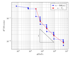
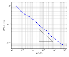
Figure 1: Test on a L-shaped domain: (left) $H^{1}(\Omega)$-error decay between the
solution $u$ and every Galerkin approximation (${\texttt{GAL}}(u)$) in
REGSOLVE and between $u$ and $U_{j}$ defined in REGSOLVE,
(right) $H^{1}(\Omega)$-error decay between $u$ and $U_{j_{\max}}$ defined
from Remark 3.6. We set
$j_{\max}=6$, and $\tau_{0}=.6$. 



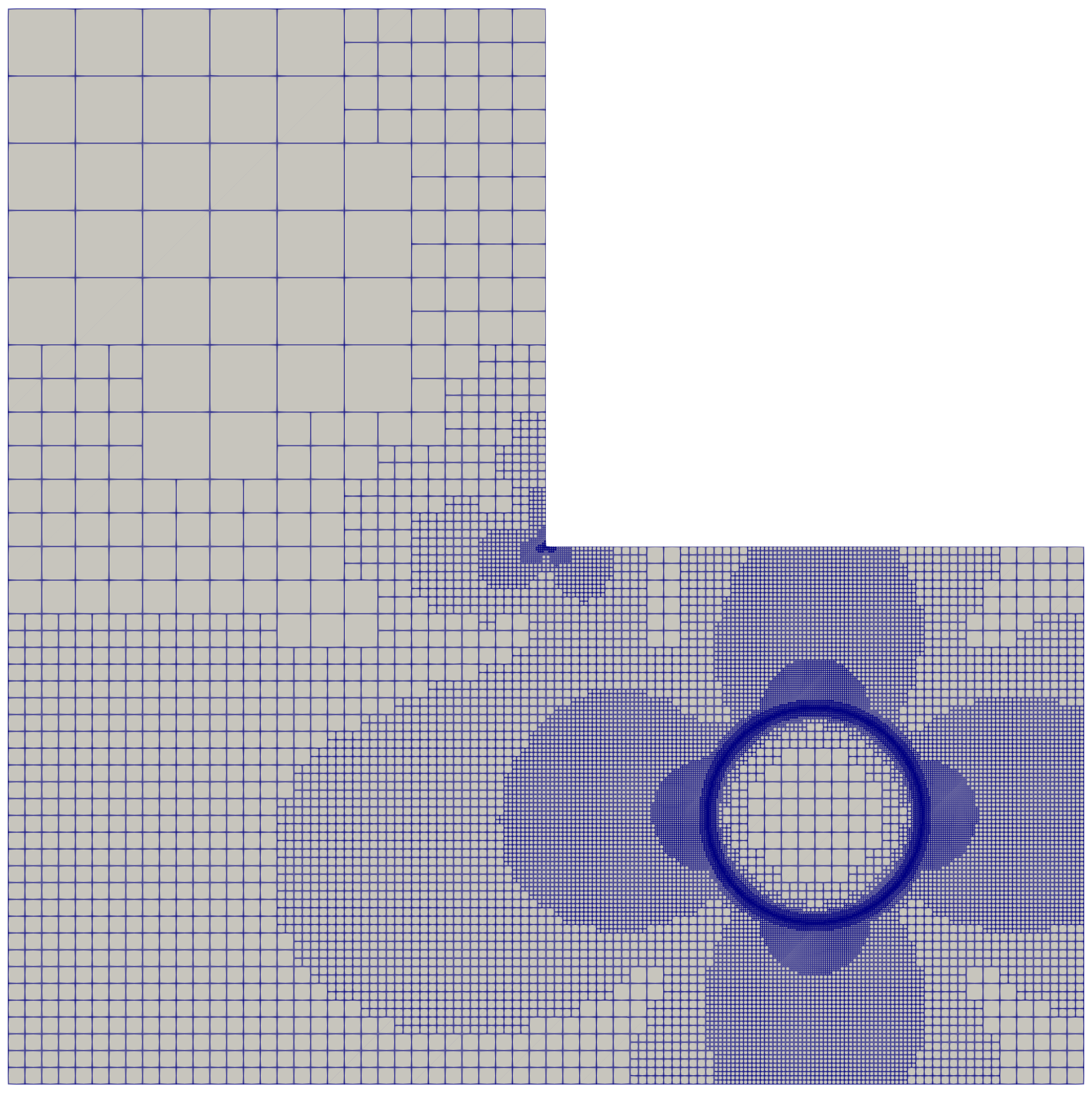
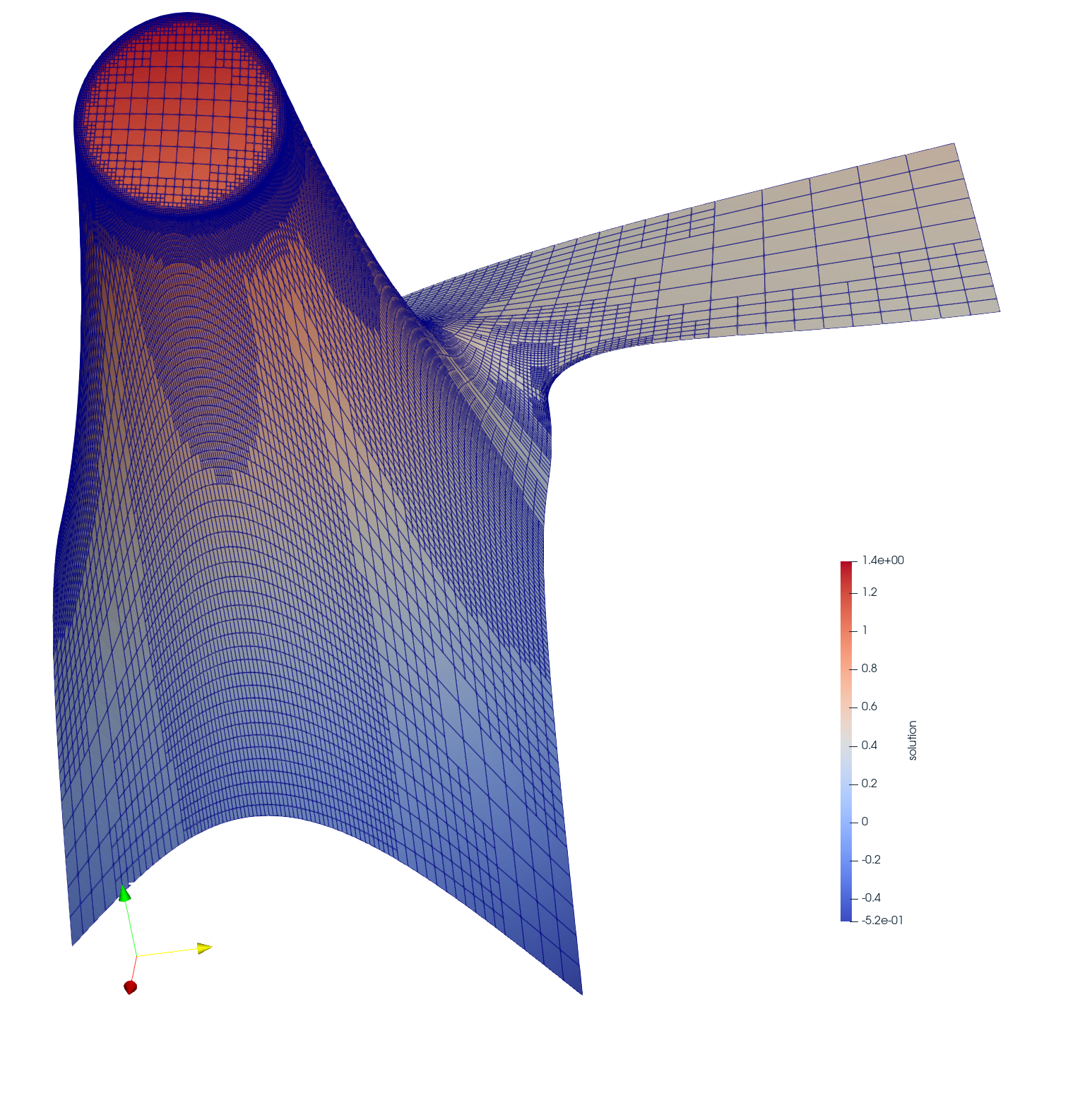
Figure 2: Test on a L-shaped domain: (left) the subdivisions of $U_{3}$ in REGSOLVE and (right) the corresponding Galerkin approximation using Tensor product $C^{1}$.




5.2 Convergence tests in the unit cube


We test our numerical algorithm in 3d by setting $\Omega=(-1,1)^{3}$ and $\gamma=\partial B_{R}(c)$ with $R=0.2$ and $c=(0.3,0.3,0.3)^{\mathtt{T}}$. We also set the data function $f=\tfrac{1}{R^{2}}$ on $\gamma$ and $g=1/|x-c|$ so that the analytic solution is given by




$$u(x)=\left\{\begin{aligned} 1/{|x-c|},&\quad\text{if }|x-c|>R,\\
1/{R},&\quad\text{if }|x-c|\leq R.\end{aligned}\right.$$



We start with an initial uniform grid $\mathcal{T}_{0}$ with the mesh size $\sqrt{3}/16$. To approximate the interface $\gamma$, we start with initial quasi-uniform coarse mesh and refine it globally 7 times so that the geometric error is small enough. For the other approximation parameters, we set $j_{\max}=5$, $\tau_{0}=1.5$, $\beta=0.8$, $\lambda=1$, $\theta=0.5$ in SOLVE and $\widetilde{\theta}=0.8$ in DATA. In Figure 3, we report the $H^{1}(\Omega)$-error against #DoFs for the following three different types of $\delta^{r}$: the radially symmetric $C^{1}$ type, the tensor product $C^{\infty}$ type generated by $\psi_{1d}(x)=\exp(1-1/(1-x^{2}))\chi_{(-1,1)}(x)$, and the tensor product $L^{\infty}$ type generated by $\psi_{1d}(x)=\tfrac{1}{2}\chi_{(-1,1)}(x)$. For each error plot, we also report the slope of the linear regression of the last five sampling points. For the choice of tensor product $C^{\infty}$, the performance is sub-optimal and close to the predicted rate $\tfrac{1}{5}$. When using radially symmetric $C^{1}$, the observed convergence rate is better than the best possible rate $\tfrac{1}{4}$. As for tensor product $L^{\infty}$, the performance is between $\tfrac{1}{4}$ and $\tfrac{1}{5}$. We also report the coarse grid and the grids for $U_{5}$, $U_{7}$ as well as the approximation $U_{7}$ using radially symmetric $C^{1}$ in Figure 4.


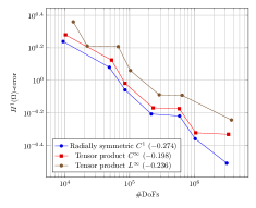
Figure 3: Tests in the unit cube: $H^{1}(\Omega)$-error decay between the solution $u$ and $U_{j}$ for $j=1,\ldots,7$ and for different choices of ${\delta^{r}}(x)$. In terms of each plot, the slope of the linear regression of the last five sampling points is reported in the legend.



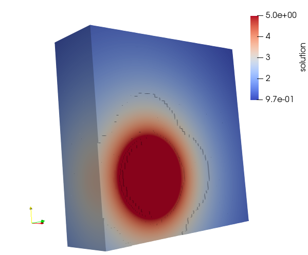
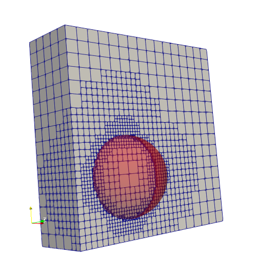
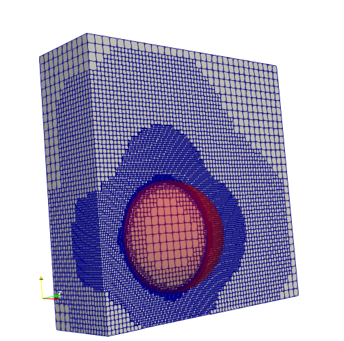
Figure 4: Tests in the unit cube: the crinkle clip ($x_{1}\leq 0.3$) of the approximation $U_{7}$ ($3741904$ DoFs) (left) as well as the subdivisions for $U_{5}$ (mid) and $U_{7}$ (right) using radially symmetric $C^{1}$. The interface $\gamma$ is marked in red.




5.3 Performance tests in the unit square


Consider $\Omega=(0,1)^{2}$, $\gamma=\partial B_{R}(c)$ with $R=0.2$ and $c=(0.3,0.3)^{{}^{\intercal}}$, $f=\tfrac{1}{R}$ and $g=\ln(|x-c|)$. Similar to the previous section, we can obtain the following exact solution




$$u(x)=\left\{\begin{aligned} -\ln(|x-c|),&\quad\text{if }|x-c|>R,\\
-\ln(R),&\quad\text{if }|x-c|\leq R.\end{aligned}\right.$$



We shall compare the performance of our numerical algorithms both in Algorithm 8 and Remark 3.6 with the algorithm without regularization; see the numerical algorithm from Section 7.2 of [17]. To be more precise, the algorithm without using the regularization is based on SOLVE by replacing the data indicator $\mathcal{D}$ with the following surrogate data indicator:




$$\widetilde{\mathcal{D}}(f,T,\mathcal{T}):=h_{T}^{1/2}\|f\|_{L^{2}(T\cap\gamma)}.$$



Using the exact solution $u$, after the $j$-th iterate of REGSOLVE in Algorithm 8 using tensor product $L^{\infty}$, we compute the $H^{1}(\Omega)$-error between $u$ and $U_{j}$, denoted by $e_{j}$. For the parameters we set $\tau_{0}=0.3$, $\beta=0.7$, $\lambda=\tfrac{1}{3}$, $\theta=\widetilde{\theta}=0.55$. Then we run the non-regularized program with the same parameters and terminate it when the energy error is smaller than $e_{j}$, denoting $\widetilde{e}_{j}$ the energy error for the corresponding output approximation. For $j=8,9,\ldots,12$. We also compute $e_{j}$ using the algorithm provided by Remark 3.6 with $j=11,\ldots,15$. Now we report those errors and the CPU times for each program against #DoFs in Figure 6. We observe that all algorithms are quasi-optimal but the algorithm from Remark 3.6 requires more DoFs.


In terms of the computation time, it turns out that
Algorithm 8 needs more time when the discrete system is small
(less than $10^{7}$) and becomes more efficient when the size of the system is
increasing.  Since the computational cost associated to the
regularized version is comparable to the one required by the non-regularized
version when computed on the same grid (see [25, Figure
7]), a fair comparison between the different AFEM algorithms
should keep into account the computational cost in terms of the attained
accuracy.


The regularized case reaches lower errors, for the same number of
degrees of freedom, but it is more expensive (due to a larger number of refined
elements around the interface $\gamma$ required by our algorithms). The
computational cost is compensated for by the higher accuracy in the largest
scale computations, where the computational cost per degree of freedom is
comparable, making the regularized approach roughly comparable to the
non-regularized one also in the AFEM context. In Figure 5,
we finally report the grid for $U_{5}$ using Algorithm 8 and
corresponding grid for the non-regularized algorithm.



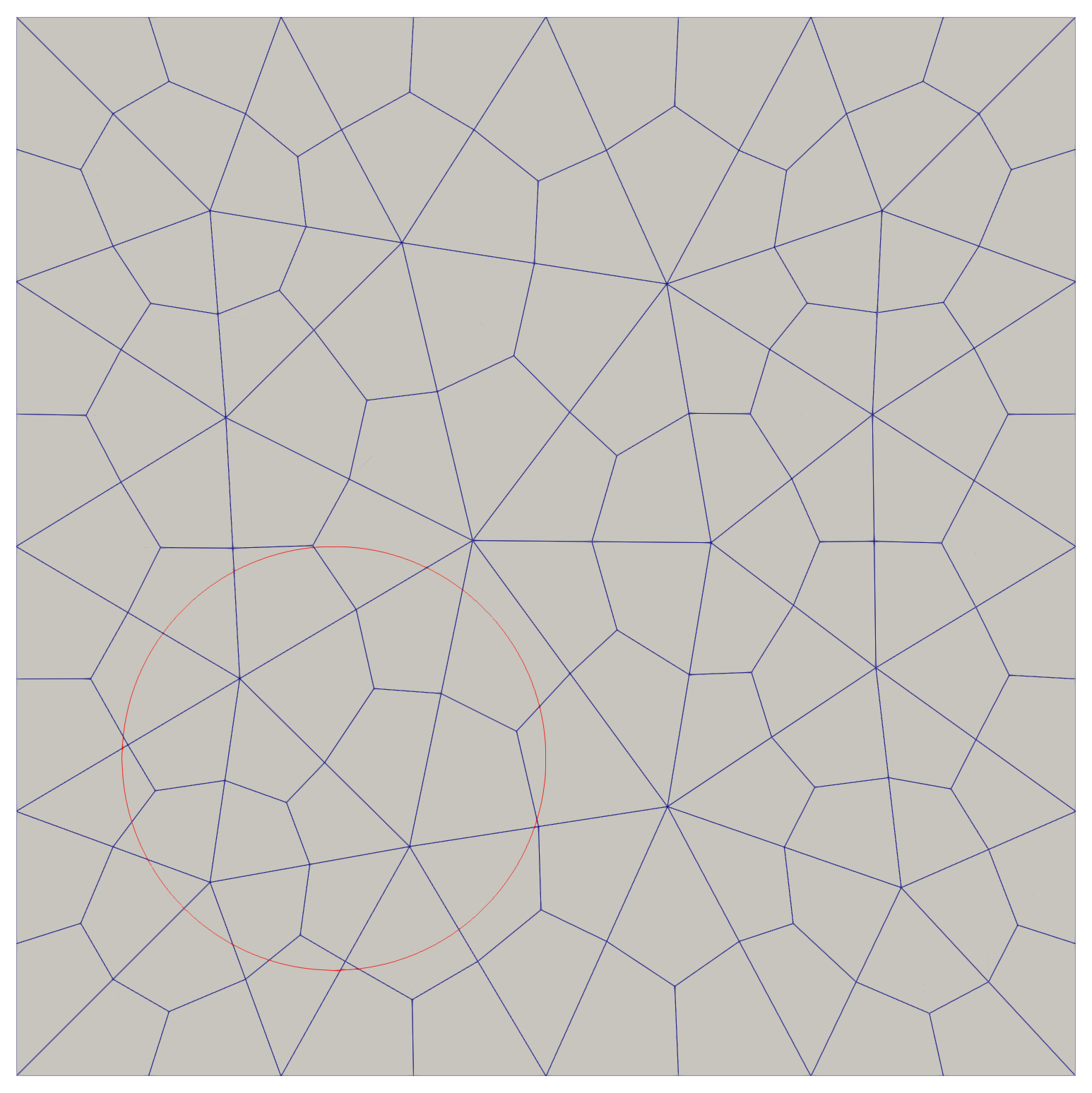
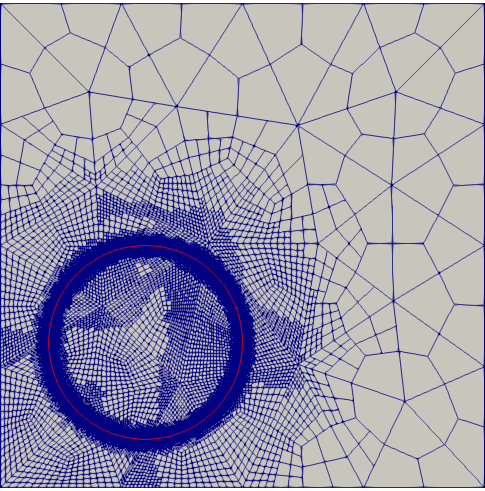
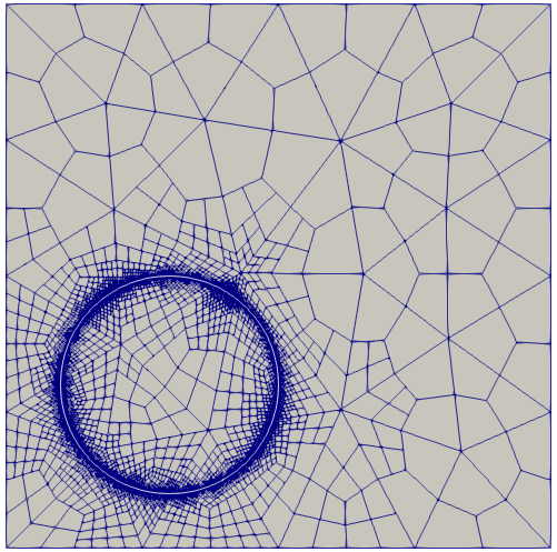
Figure 5: Tests on a square: (left) the unstructured coarse mesh $\mathcal{T}_{0}$, (center) the subdivision for $U_{5}$, and (right) the corresponding subdivision using non-regularized algorithm.


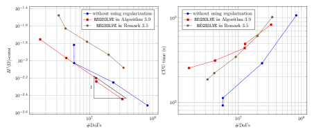
Figure 6: Tests on a square: (left) $\|U_{j}-u\|_{H^{1}(\Omega)}$ using REGSOLVE with tensor product $L^{\infty}$ for $j=8,\ldots$ and the corresponding $H^{1}(\Omega)$-error decay without using the regularization; (right) computational time against #nDoFs for two adaptive algorithms. We note that the sampling points for the non-regularized algorithm at $j=10$ and $11$ are so closed that they overlap with each other.



6 Conclusion and outlook


We have proposed an adaptive finite element algorithm to approximate the solutions of elliptic problems with rough data approximated by regularization. Such problems are relevant in many applications ranging from fluid-structure interaction, to the modeling of biomedical applications with complex embedded domains or networks.


Our approach builds on classical results for adaptive finite element theory for $H^{-1}$ data, and for $L^{2}$ data. In particular, we analyze the regularization of line Dirac delta distributions via convolutions with compactly supported approximated Dirac delta functions, with radius $r$. What characterizes the regularization process is that, even if the resulting forcing term is as regular as desired – at fixed $r$ – its regularity does not hold uniformly with respect to $r$.


This observation suggests that one could exploit the knowledge of the asymptotic behavior of the data regularity with respect to $r$ to construct an algorithm that a priori refines around the rough part of the forcing term, in a way that guarantees quasi optimal convergence, at least in the two dimensional case.


The resulting approximation error is split into a regularization error for $u$ and the finite element approximation error for the regularized ${\mathtt{u}^{r}}$. In this work we show how to control the dependencies between these two errors and provide an algorithm in which the error decay in the energy norm is quasi-optimal in two dimensional space and sub-optimal in three dimensional space.


Our findings are specific for the co-dimension one case, but could be easily extended to the co-dimension zero case, where the dependency of the regularity on $r$ disappears naturally, due to the intrinsic $L^{2}$ nature of the resulting forcing term.



Appendix A Proof of Proposition 4.1



Given a cell $T\in\mathcal{G}(\mathcal{T},r)$, $T$ will be marked to refine in ${\texttt{INTERFACE}}(\mathcal{T},r)$ if $h_{T}>\tfrac{r}{2}$. This also holds in the process of
$\mathcal{T}^{*}={\texttt{INTERFACE}}(\mathcal{T}_{0},r)$ as the parents of $T$ also satisfy the marking criteria. So $\#(\widetilde{\mathcal{T}})-\#(\mathcal{T})\leq\#(\mathcal{T}^{*})-\#(\mathcal{T}_{0})$. For any nonnegative integer $j$, denote $\widetilde{\mathcal{T}}_{0}=\mathcal{T}_{0}$ and $\widetilde{\mathcal{T}}_{j}$ the conforming refinement of $\mathcal{T}_{j-1}$ by bisecting cells in $\mathcal{G}(\gamma,\widetilde{\mathcal{T}}_{j-1})$ once. Let $j_{r}$ be the smallest integer satisfying $\mathcal{G}_{j}:=\operatorname*{diam}(\mathcal{G}(\gamma,\widetilde{\mathcal{T}}_{j}))<r$. Clearly, $\widetilde{\mathcal{T}}_{j_{r}}$ is a refinement of $\mathcal{T}^{*}$ and it suffices to show that



(37)

$$\#(\widetilde{\mathcal{T}}_{j_{r}})-\#(\mathcal{T}_{0})\lesssim r^{1-d}.$$





According to the assumption (25), we apply the quasi-uniformity of $\mathcal{G}(\gamma,\mathcal{T}_{0})$ as well as the relation $|\widetilde{T}|=q^{-j}|T|$ for $\widetilde{T}\in\mathcal{G}_{j}$ and its parent $T\in\mathcal{\mathcal{missing}}T_{0}$ to get
$\#(\mathcal{G}_{j})\lesssim q^{i(1-1/d)}.$
Summing up this estimate for $j=0,\ldots,j_{r}-1$ to obtain that




$$\#(\widetilde{\mathcal{T}}_{j_{r}})-\#(\mathcal{T}_{0})\leq\sum_{j=0}^{j_{r}-1}\#(\mathcal{G}_{j})\lesssim q^{(j_{r}+1)(1-1/d)}.$$



The target estimate (37) follows from the fact $q^{-j_{r}/d}\sim r$ with the hidden constants depending on $q,\mathcal{T}_{0}$ and $\gamma$.




Appendix B Proof of Lemma 4.7



We split the proof in the following steps.


$$1$$ Suppose that there are totally $N$ iterations executed in the while loop when ${{\texttt{GREEDY}}}(\widetilde{\mathcal{T}},F^{r},\tau)$ terminates. We denote with $\{T^{i}\}_{i=0}^{N}$ the marked cells in the sequence and set $\mathcal{T}^{i}={\texttt{REFINE}}(\mathcal{T}^{i-1},\{T^{i-1}\})$ for $i=1,\ldots,N$ and $\mathcal{T}^{0}=\widetilde{\mathcal{T}}$. Let




$$\delta:=d(F^{r},T^{N-1},\mathcal{T}^{N-1})=\text{argmax}\{d(F^{r},T,\mathcal{T}^{N-1}):T\in\mathcal{T}^{N-1}\}.$$



Noting that for $0\leq i\leq N-1$, there exists $T^{\prime}\in\mathcal{T}^{i}$ such that $T^{N-1}\subset T$. Clearly, by the definition of $T^{i}$, we have



(38)

$$d(F^{r},T^{i},\mathcal{T}^{i})\geq d(F^{r},T^{\prime},\mathcal{T}^{i})\geq d(F^{r},T^{N-1},\mathcal{T}^{N-1})=\delta.$$



According to the definition of $T^{N-1}$, we also get



(39)

$$\tau\leq\mathcal{D}(F^{r},\mathcal{T}^{N-1})\leq\delta\sqrt{\#(\mathcal{T}^{N-1})}.$$





$$2$$ Since $F^{r}$ is supported in $U_{r}$, $T^{i}\subset U_{cr}$ for some constant $c\geq 1$ depending on ${c_{\texttt{sr}}}$. Let $\mathcal{B}_{j}\subset\{T^{i}\}$ be the set satisfying



(40)

$$2^{-(j+1)}|U_{cr}|<|T^{i}|\leq 2^{-j}|U_{cr}|,\quad j\geq 0.$$



Due to the refinement process from $\mathcal{T}^{i}$ to $\mathcal{T}^{i+1}$, $\{T^{i}\}$ are distinct from each other. This implies that by summing up the first inequality of (40) for all $T^{i}\in\mathcal{B}_{j}$, we obtain $\#(\mathcal{B}_{j})<2^{j+1}$. using the second inequality of (40) as well as (39), we realize that for $T^{i}\in\mathcal{B}_{j}$,




$$\delta\leq d(F^{r},T^{i},\mathcal{T}^{i})=|T^{i}|^{1/d}\|F^{r}\|_{L^{2}(T^{i})}\leq 2^{-j/d}|U_{cr}|^{1/d}\|F^{r}\|_{L^{2}(T^{i})}.$$



We square the above estimate and sum it up for all $T^{i}\in\mathcal{B}_{j}$ to obtain




$$\delta^{2}\#(\mathcal{B}_{j})\leq 2^{-2j/d}|U_{cr}|^{2/d}\|F^{r}\|_{L^{2}(U_{cr})}^{2}$$



The above estimate together with $\#(\mathcal{B}_{j})<2^{j+1}$ implies that the total marked cells can be estimated with



(41)

$$N=\sum_{j\geq 0}\#(\mathcal{B}_{j})\leq\sum_{j\geq 0}\min(2^{-2j/d}\delta^{-2}|U_{cr}|^{2/d}\|F^{r}\|_{L^{2}(U_{cr})}^{2},2^{j+1}).$$





$$3$$ Since the first term of the above minimum decreases with respect to $j$, we set $j_{0}$ be the smallest integer such that



(42)

$$2^{j_{0}+1}>2^{-2j_{0}/d}\delta^{-2}|U_{cr}|^{2/d}\|F^{r}\|_{L^{2}(U_{cr})}^{2}.$$



Simplifying this relation for $j_{0}$ we get




$$2^{-j_{0}}\lesssim\bigg{(}\delta^{-1}|U_{cr}|^{1/d}\|F^{r}\|_{L^{2}(U_{cr})}\bigg{)}^{-2d/(2+d)}.$$



If $j_{0}>0$, (42) is violated for $j=j_{0}-1$ and we can deduce that




$$2^{j_{0}}\lesssim\bigg{(}\delta^{-1}|U_{cr}|^{1/d}\|F^{r}\|_{L^{2}(U_{cr})}\bigg{)}^{2d/(2+d)}.$$



Inserting the above two estimate in (41), we have



(43)

$$N
\leq\sum_{j<j_{0}}2^{j+1}+\delta^{-2}|U_{cr}|^{2/d}\|F^{r}\|_{L^{2}(U_{cr})}^{2}\sum_{j\geq j_{0}}2^{-2j/d}$$






$$\lesssim 2^{j_{0}}+\bigg{(}\delta^{-1}|U_{cr}|^{1/d}\|F^{r}\|_{L^{2}(U_{cr})}\bigg{)}^{2}2^{-2j_{0}/d}$$





$$\lesssim\bigg{(}\delta^{-1}|U_{cr}|^{1/d}\|F^{r}\|_{L^{2}(U_{cr})}\bigg{)}^{2d/(2+d)}$$






$$4$$ We shall further bound the above estimate by considering the $L^{2}(U_{cr})$-norm of $F^{r}$. In fact,




$$\|F^{r}\|_{L^{2}(U_{cr})}^{2}
=\int_{U_{cr}}\bigg{(}\int_{\gamma}\delta^{r}(x-y)f(y)\,\mbox{\rm d}y\bigg{)}^{2}\,\mbox{\rm d}x$$






$$\leq\frac{1}{r^{2d}}\|\psi\|_{L^{\infty}(\mathbb{R}^{d})}^{2}\|f\|_{L^{\infty}(\gamma)}^{2}\int_{U_{cr}}|B_{r}(x)\cap\gamma|^{2}\,\mbox{\rm d}x$$





$$\leq C\frac{1}{r^{2d}}\|\psi\|_{L^{\infty}(\mathbb{R}^{d})}^{2}\|f\|_{L^{\infty}(\gamma)}^{2}r^{2(d-1)+1}\lesssim r^{-1}\|f\|_{L^{\infty}(\gamma)}^{2},$$



where for the second inequality above we used the fact that $|B_{r}(x)\cap\gamma|\lesssim r^{d-1}$ for $x\in D_{cr}$ and $|D_{cr}|\sim|\gamma|r$.


$$5$$ Combining the results from Step 3 and 4 to deduce that



(44)

$$N\lesssim\delta^{-2d/(2+d)}r^{(2-d)/(2+d)}\|f\|_{L^{\infty}(\gamma)}^{2d/(2+d)},$$



where the hidden constant above depends on ${c_{\texttt{sr}}},\gamma,d$ and $\psi$. On the other hand, the complexity assumption (20) implies that




$$\#(\mathcal{T}^{N-1})-\#(\mathcal{T}^{0})\leq{C_{\texttt{com}}}N.$$



Hence the above relation together with (44) and (39) concludes that




$$\tau
\leq\delta\sqrt{\#(\mathcal{T}^{N-1})}$$






$$\lesssim\frac{\sqrt{\#(\mathcal{T}^{0})+{C_{\texttt{com}}}N}}{N^{(2+d)/(2d)}}r^{1/d-1/2}\|f\|_{L^{\infty}(\gamma)}\lesssim N^{-1/d}r^{1/d-1/2}\|f\|_{L^{\infty}(\gamma)},$$



which implies the target estimate.


$$6$$ If $j_{0}=0$, we directly get $\delta^{-1}|U_{cr}|^{1/d}\|F^{r}\|_{L^{2}(U_{cr})}\lesssim 1$. Starting form (41), we apply the result in Step 4 to write




$$N
\lesssim\delta^{-2}|U_{cr}|^{2/d}\|F^{r}\|_{L^{2}(U_{cr})}^{2}\sum_{j\geq 0}2^{-2j/d}$$






$$\lesssim\delta^{-2}|U_{cr}|^{2/d}\|F^{r}\|_{L^{2}(U_{cr})}^{2}$$





$$\leq\delta^{-1}|U_{cr}|^{1/d}\|F^{r}\|_{L^{2}(U_{cr})}\lesssim\delta^{-1}r^{1/d-1/2}\|f\|_{L^{\infty}(\gamma)}.$$



Therefore, we again obtain the target estimate following the argument in Step 5. The proof is complete.

References

[1]A. Allendes, E. Otárola, and A. J. Salgado, A posteriori error
estimates for the stokes problem with singular sources, Computer Methods in
Applied Mechanics and Engineering, 345 (2019), pp. 1007–1032.
[2]G. Alzetta and L. Heltai, Multiscale modeling of fiber reinforced
materials via non-matching immersed methods, Computers & Structures, 239
(2020), p. 106334.
[3]D. Arndt, W. Bangerth, B. Blais, M. Fehling, R. Gassmöller,
T. Heister, L. Heltai, U. Köcher, M. Kronbichler, M. Maier, et al., The deal. ii library, version 9.3, Journal of Numerical Mathematics, 29
(2021), pp. 171–186.
[4]D. Arndt, W. Bangerth, D. Davydov, T. Heister, L. Heltai, M. Kronbichler,
M. Maier, J.-P. Pelteret, B. Turcksin, and D. Wells, The deal.II
finite element library: Design, features, and insights, Computers &
Mathematics with Applications, 81 (2021), pp. 407–422.
[5]R. E. Bank and A. Weiser, Some a posteriori error estimators for
elliptic partial differential equations, Math. Comp., 44 (1985),
pp. 283–301.
[6]S. Berrone, A. Bonito, R. Stevenson, and M. Verani, An optimal
adaptive fictitious domain method, Mathematics of Computation, 88 (2019),
pp. 2101–2134.
[7]S. Bertoluzza, A. Decoene, L. Lacouture, and S. Martin, Local error
estimates of the finite element method for an elliptic problem with a dirac
source term, Numerical Methods for Partial Differential Equations, 34
(2017), pp. 97–120.
[8]P. Binev, W. Dahmen, and R. DeVore, Adaptive finite element methods
with convergence rates, Numer. Math., 97 (2004), pp. 219–268.
[10]D. Boffi and L. Gastaldi, A finite element approach for the immersed
boundary method, Comput. & Structures, 81 (2003), pp. 491–501.
In honour of Klaus-Jürgen Bathe.
[11]D. Boffi and L. Gastaldi, On the existence and the uniqueness of the
solution to a fluid-structure interaction problem, Journal of Differential
Equations, 279 (2021), pp. 136–161.
[12]A. Bonito, R. A. DeVore, and R. H. Nochetto, Adaptive finite element
methods for elliptic problems with discontinuous coefficients, SIAM J.
Numer. Anal., 51 (2013), pp. 3106–3134.
[13]A. Bonito and R. H. Nochetto, Quasi-optimal convergence rate of an
adaptive discontinuous Galerkin method, SIAM J. Numer. Anal., 48 (2010),
pp. 734–771.
[14]J. M. Cascon, C. Kreuzer, R. H. Nochetto, and K. G. Siebert, Quasi-optimal convergence rate for an adaptive finite element method, SIAM
J. Numer. Anal., 46 (2008), pp. 2524–2550.
[15]D. Cerroni, F. Laurino, and P. Zunino, Mathematical analysis, finite
element approximation and numerical solvers for the interaction of 3d
reservoirs with 1d wells, GEM - International Journal on Geomathematics, 10
(2019).
[16]P. G. Ciarlet, The finite element method for elliptic problems,
vol. 40 of Classics in Applied Mathematics, Society for Industrial and
Applied Mathematics (SIAM), Philadelphia, PA, 2002.
Reprint of the 1978 original [North-Holland, Amsterdam; MR0520174 (58
#25001)].
[17]A. Cohen, R. DeVore, and R. H. Nochetto, Convergence rates of AFEM
with data, Found. Comput. Math., 12 (2012), pp. 671–718.
[18]W. Dörfler, A convergent adaptive algorithm for Poisson’s
equation, SIAM J. Numer. Anal., 33 (1996), pp. 1106–1124.
[19]W. Dörfler and R. H. Nochetto, Small data oscillation implies
the saturation assumption, Numer. Math., 91 (2002), pp. 1–12.
[20]A. Ern and J.-L. Guermond, Theory and practice of finite elements,
vol. 159 of Applied Mathematical Sciences, Springer-Verlag, New York, 2004.
[21]P. Grisvard, Elliptic problems in nonsmooth domains, vol. 24 of
Monographs and Studies in Mathematics, Pitman (Advanced Publishing Program),
Boston, MA, 1985.
[22]L. Heltai and A. Caiazzo, Multiscale modeling of vascularized
tissues via nonmatching immersed methods, Int. J. Numer. Methods Biomed.
Eng., 35 (2019), pp. e3264, 32.
[23]L. Heltai, A. Caiazzo, and L. O. Müller, Multiscale coupling of
one-dimensional vascular models and elastic tissues, Annals of Biomedical
Engineering, (2021).
[24]L. Heltai and F. Costanzo, Variational implementation of immersed
finite element methods, Comput. Methods Appl. Mech. Engrg., 229/232 (2012),
pp. 110–127.
[25]L. Heltai and W. Lei, A priori error estimates of regularized
elliptic problems, Numer. Math., 146 (2020), pp. 571–596.
[26]L. Heltai and N. Rotundo, Error estimates in weighted sobolev norms
for finite element immersed interface methods, Computers & Mathematics
with Applications, 78 (2019), pp. 3586–3604.
[27]B. Hosseini, N. Nigam, and J. M. Stockie, On regularizations of the
Dirac delta distribution, J. Comput. Phys., 305 (2016), pp. 423–447.
[28]P. Houston and T. P. Wihler, Discontinuous galerkin methods for
problems with dirac delta source, Mathematical Modelling and Numerical
Analysis, 46 (2012), pp. 1467–1483.
[29]R. Krause and P. Zulian, A parallel approach to the variational
transfer of discrete fields between arbitrarily distributed unstructured
finite element meshes, SIAM Journal on Scientific Computing, 38 (2016),
pp. C307–C333, https://doi.org/10.1137/15M1008361,
https://doi.org/10.1137/15M1008361.
[30]C. Kreuzer and A. Veeser, Oscillation in a posteriori error
estimation, Numerische Mathematik, 148 (2021), pp. 43–78.
[31]H. Li, X. Wan, P. Yin, and L. Zhao, Regularity and finite element
approximation for two-dimensional elliptic equations with line dirac
sources, Journal of Computational and Applied Mathematics, 393 (2021),
p. 113518.
[32]F. Millar, I. Muga, S. Rojas, and K. G. V. der Zee, Projection in
negative norms and the regularization of rough linear functionals, 2021,
https://arxiv.org/abs/2101.03044.
[33]W. F. Mitchell, A comparison of adaptive refinement techniques for
elliptic problems, ACM Trans. Math. Software, 15 (1989), pp. 326–347
(1990).
[34]R. Mittal and G. Iaccarino, Immersed boundary methods, in Annual
review of fluid mechanics. Vol. 37, vol. 37 of Annu. Rev. Fluid Mech.,
Annual Reviews, Palo Alto, CA, 2005, pp. 239–261.
[35]P. Morin, R. H. Nochetto, and K. G. Siebert, Data oscillation and
convergence of adaptive fem, SIAM Journal on Numerical Analysis, 38 (2000),
pp. 466–488.
[36]R. H. Nochetto, Pointwise a posteriori error estimates for elliptic
problems on highly graded meshes, Mathematics of computation, 64 (1995),
pp. 1–22.
[37]R. H. Nochetto, K. G. Siebert, and A. Veeser, Theory of adaptive
finite element methods: an introduction, in Multiscale, nonlinear and
adaptive approximation, Springer, Berlin, 2009, pp. 409–542.
[38]C. S. Peskin, The immersed boundary method, Acta Numer., 11 (2002),
pp. 479–517.
[39]D. D. Silva, F. Ferrari, and S. Salsa, Perron’s solutions for
two-phase free boundary problems with distributed sources, Nonlinear
Analysis: Theory, Methods & Applications, 121 (2015), pp. 382–402.
[40]R. Stevenson, An optimal adaptive finite element method, SIAM J.
Numer. Anal., 42 (2005), pp. 2188–2217.
[41]R. Stevenson, Optimality of a standard adaptive finite element
method, Found. Comput. Math., 7 (2007), pp. 245–269.
[42]R. Stevenson, The completion of locally refined simplicial
partitions created by bisection, Math. Comp., 77 (2008), pp. 227–241.
[43]J.-P. Suarez, G. B. Jacobs, and W.-S. Don, A high-order dirac-delta
regularization with optimal scaling in the spectral solution of
one-dimensional singular hyperbolic conservation laws, SIAM Journal on
Scientific Computing, 36 (2014), pp. A1831–A1849.
[44]A.-K. Tornberg, Multi-dimensional quadrature of singular and
discontinuous functions, BIT, 42 (2002), pp. 644–669.