A spatio-temporal analysis of NO₂ concentrations during the Italian 2020 COVID-19 lockdown

Abstract

When a new environmental policy or a specific intervention is taken in order to improve air quality, it is paramount to assess and quantify - in space and time - the effectiveness of the adopted strategy. The lockdown measures taken worldwide in 2020 to reduce the spread of the SARS-CoV-2 virus can be envisioned as a policy intervention with an indirect effect on air quality. In this paper we propose a statistical spatio-temporal model as a tool for intervention analysis, able to take into account the effect of weather and other confounding factors, as well as the spatial and temporal correlation existing in the data. In particular, we focus here on the 2019/2020 relative change in nitrogen dioxide (NO₂) concentrations in the north of Italy, for the period of March and April during which the lockdown measure was in force. As an output, we provide a collection of weekly continuous maps, describing the spatial pattern of the NO₂ 2019/2020 relative changes. We found that during March and April 2020 most of the studied area is characterized by negative relative changes (median values around -25%), with the exception of the first week of March and the fourth week of April (median values around 5%). As these changes cannot be attributed to a weather effect, it is likely that they are a byproduct of the lockdown measures.

1 Introduction

In the last decades a large number of initiatives have been taken in European countries in order to reduce air pollution and its adverse effects on human health. This is for example the case of low emission zones or congestion charge introduced in urban areas [see e.g., Fassò, 2013, Holman et al., 2015, Maranzano et al., 2020], of more stringent limits on the content of sulfur in marine fuels [e.g., Grange and Carslaw, 2019] or of new air pollution control regulations [e.g., Font and Fuller, 2016, Han et al., 2021], among others [see Burns et al., 2020, for a review]. A crucial issue in air quality management is the assessment of the efficacy of a specific intervention or a new environmental policy. In particular, quantifying the effective changes in pollutant concentrations due to the adopted strategy can be difficult because of the complexity of air pollution dynamics, strongly depending on weather conditions. Moreover, when the intervention is time-delimited and characterizes different areas, it may be interesting to evaluate the variability in space and time of its effect, if any.

The lockdown measures adopted by many countries in 2020 in order to to prevent the spread of the SARS-CoV-2 virus can be considered as a policy intervention, with a possible indirect effect on air quality. In this regard, the main focus is on assessing how the lockdown affected air pollution levels, in particular after controlling for meteorology, long term trend and other confounding factors. The literature on this topic is obviously quite recent but already large, as discussed in the two recent systematic reviews by Gkatzelis et al. [2021] and Rana et al. [2021].

In this paper, we propose a new statistical modeling approach for assessing and quantifying the effectiveness of a policy intervention on air quality. In particular, our statistical model is defined for daily differences of pollutant concentrations and has a spatio-temporal specification which gives us the possibility to estimate in space and time the relative change in air pollution levels. We show here an application of our modelling strategy for nitrogen dioxide (NO₂) concentrations in northern Italy during the months of the first Italian lockdown (March and April 2020) as compared to 2019. In early 2020, Italy was the first European country to adopt strict lockdown measures [Remuzzi and Remuzzi, 2020]. Starting from late February 2020, people were banned from travelling and all the non essential socio-economic activities were stopped. These restrictive measures were initially adopted in some limited municipalities in northern Italy and then were extended to the entire country with the national lockdown in force since March 8${}^{\text{th}}$, 2020 [Malpede and Percoco, 2020, Sanfelici, 2020]. The restrictions caused, incidentally, a strong decrease in anthropogenic emissions of the main air pollutants, especially for some sectors such as road transport and aviation.

Several environmental studies revealed that restrictions on mobility during the lockdown had a positive effect on NO₂ levels, even if not homogeneously across the considered spatial domains. For example, the broadly-publicized data from the Copernicus Sentinel-5P satellite [Dutta et al., 2021, Muhammad et al., 2020, Bar et al., 2021] recorded for NO₂ a sharp drop, in the range 20–55%, during January – April 2020 compared to 2019 in many cities in China, India, Western Europe and United States. With regards to Italy, Bauwens et al. [2020] found the average TROPOMI NO₂ column during the lockdown period in 2020 to be between 38 ($\pm$ 10%) lower than during the same period in 2019 in Milan. Similarly, Cersosimo et al. [2020] reported a general decrease in NO₂ levels over the Po Valley during the lockdown using both satellite and in situ measurements. For the city of Rome and its surroundings, Bassani et al. [2021] documented a 2019 vs 2020 reduction of 50% in NO₂ concentrations using surface measurements from urban traffic stations. The NO₂ decrease for the city of Rome was also documented in Kumari and Toshniwal [2020]. Finally, a general decrease in the NO₂ levels for three cities in Tuscany region was described by Donzelli et al. [2020], for Reggio Emilia by Marinello et al. [2021] and for Naples by Sannino et al. [2021]. The main weakness of the aforementioned studies consists in their descriptive approach, based on the direct comparison of pollutant concentrations before and after the lockdown or between the lockdown period and the corresponding period of the previous year(s). In other words, these studies make no attempt to adjust for the effect of meteorological conditions which can be adverse or favorable to pollutant dispersion. In this regard, it is worth to note that the first quarter of 2020 experienced exceptional weather conditions with also stronger positive temperatures anomalies over Europe [Barré et al., 2020, van Heerwaarden et al., 2021].

A number of studies approached the problem of assessing the lockdown effects on air quality using chemical transport models (CTM) in order to compare model forecasts under the business-as-usual (BAU) emission scenario with the observed ground-level measurements or with the expected concentrations computed under a COVID-19 pandemic scenario with reduced emissions [see e.g., Barré et al., 2020, Menut et al., 2020, Piccoli et al., 2020, Putaud et al., 2020, Zhe et al., 2021]. In any case, the use of deterministic models poses a number of practical and conceptual difficulties. First, collecting the needed input data (e.g., emission inventories and meteorology data) is far from straightforward. Second, deterministic models are complex to be run and are not able to properly assess the uncertainty of the results.

Another substantial research line is represented by model-based studies. In this context historical measurement data from previous years (or from the pre-lockdown period) are used to run machine learning algorithms [see e.g., Barré et al., 2020, Diémoz et al., 2021, Keller et al., 2021, Kim et al., 2021, Grange et al., 2021, Petetin et al., 2020, Granella et al., 2021] or to estimate statistical models, as multiple linear regression models [e.g., Bao and Zhang, 2020, Dacre et al., 2020, Hoermann et al., 2021], Generalized Additive Models [e.g., EEA, 2020, Carlos et al., 2020, Solberg et al., 2021a, b] or Autoregressive Integrated Moving Average models [e.g., Tyagi et al., 2020]. The fitted model is then used to predict concentrations for 2020 (or for the post-lockdown period) under the BAU (or counterfactual) scenario, i.e., assuming that the lockdown did not take place. In order to correct for the weather effect and temporal trends, meteorological and time variables are included in the model as linear or non-linear effects. The differences between the predictions, derived from the estimated model, and the observed concentrations (i.e., the out-of-sample prediction errors) are then used to evaluate the effect of the lockdown restrictions. Other papers adopt a different modeling approach and define the counterfactual by using data from cities not subject to lockdown restrictions; then difference-in-differences (DID) models are used to estimate the relative change in pollutant concentrations in the treatment group (locked-down cities) compared with the control group (non-locked-down cities) [see e.g., He et al., 2020, Wang et al., 2021]. An extension of the DID method is proposed in Zheng et al. [2021] with the aim of computing the would-be average concentrations without the COVID-19 pandemic by removing the meteorological confounding and accounting for the temporal trend. Another modeling strategy makes use of time series model or dynamic panel data model, where pollutant concentrations, measured in 2020 and possibly in previous years, represent the response variable. The lockdown effect is included as a time-dependent dummy variable in the set of regressors, together with meteorological and time variables [see e.g., Bao and Zhang, 2020, Beloconi et al., 2021, Cameletti, 2020]. In this case the effectiveness of the lockdown is evaluated by means of the lockdown dummy coefficient and its interaction with time or other regressors.

Whatever the adopted model-based strategy is, pollutant concentrations time series can be analysed separately for each monitoring station or jointly. The second solution leads to more efficient parameter estimates and a better predictive capability because of the larger amount of available data. More importantly, when measurements come from several spatial sites it is convenient to account also for spatial correlation, besides the temporal one, for explaining any residual variability. This is a standard and well-established option in air pollution modeling [see e.g., Finazzi et al., 2013, Sahu et al., 2006, Lee et al., 2016] given that nearby monitoring stations are expected to show similar pollutant concentrations values. As far as we know, Beloconi et al. [2021] is the only study which implements a spatio-temporal model for evaluating the effect of COVID-19 lockdown on air quality, while all the other papers fail to consider the spatial correlation. However, in Beloconi et al. [2021] the analysis of the impact of the lockdown is limited at the single point stations and no continuous maps are provided for the entire region of interest.

In this paper, using a spatio-temporal statistical model, we aim to produce spatio-temporal maps showing continuously in space and across time the impact of the lockdown on air pollution. We expect these highly spatially resolved maps to help in assessing if the lockdown effect was homogeneous in the considered area or was more consistent in particular zones. Having this goal in mind, we modeled the 2019/2020 daily differences of NO₂ concentrations (in March and April), rather than jointly modeling the data available for the two years. This makes it possible to focus on the change occurred between 2019 and 2020 in the NO₂ levels, while still accounting for the effect of meteorology. In particular, by including a spatial stochastic component, our model is able to take care of the spatial correlation between observations and generate spatially continuous prediction surfaces, also where no ground-monitoring stations are available and in remote or mountainous areas [Diémoz et al., 2021]. The model we propose is applied here to the Italian COVID-19 case study but it is a general modeling approach that can be implemented anytime it is necessary to evaluate the effect of an intervention on an output variable with a spatio-temporal dimension.

The paper is structured as follows: in Section 2 we introduce the study domain and the input data. Then, in Section 3 the proposed spatio-temporal regression model is described; details are also provided with respect to the prediction phase of the analysis. Finally, in Section 4 we describe the main results of our analysis with particular attention to the prediction maps. Section 5 concludes the paper.

2 Data material

2.1 Monitoring sites and air pollution data

In this study we focused on the Italian COVID-19 lockdown period (from March $1^{\text{st}}$ to 30 April $30^{\text{th}}$, 2020), corresponding to 10 weeks of daily observations. The 2019 and 2020 raw NO₂ hourly data (expressed as $\mu g/m^{3}$), together with monitoring stations metadata, were extracted from the national database used to store and process the Italian Air quality measurements [SNPA, 2020]. The hourly data were measured at stations operated by the local Regional Environmental Protection Agencies, following the European standards EN 14211:2012 for NO, NO₂, and NO${}_{\text{X}}$ [CEN-TC 264, 2012]. All ground concentrations were fully validated following internal quality assurance and quality control standard procedures.

Daily averages were computed provided that a daily 75% data coverages was achieved (i.e., at least 18 valid hourly records out of 24). The input dataset for our analysis regards 200 monitoring sites with a low proportion of missing data ($<25\%$ per station) and distributed across 8 regions or autonomous provinces in the north of Italy (Valle d’Aosta 4 stations, Piedmont 17, Veneto 32, Lombardy 55, Autonomous province of Trento 5, Friuli Venezia Giulia 12, Autonomous province of Bozen 5, Emilia Romagna 36) plus Tuscany region in the centre of Italy (with 34 stations). The spatial distribution of the selected stations is illustrated in Figure 1. The monitoring stations cover urban (123 stations), suburban (39) and rural (38) areas. At the time of the analysis, we were not able to access to the NO₂ data from Liguria region (the western region filled in gray in the map in Figure 1).

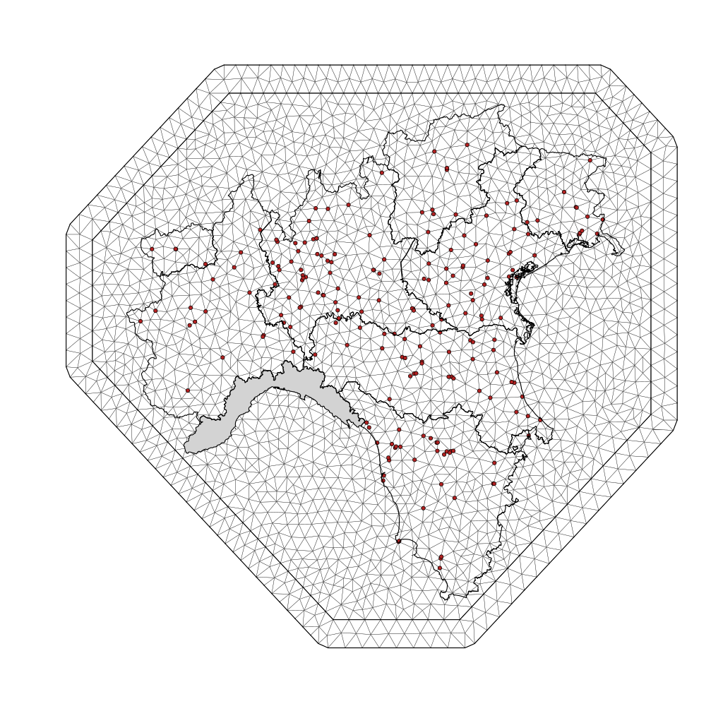
Figure 1: Spatial distribution of the monitoring sites for $\text{NO}_{2}$ concentrations (red points) and mesh adopted for the implementation of the spatio-temporal model described in Section 3.

The investigated area is characterized: in the north, by remote and relatively pristine areas with the high peaks of the Alps mountain system; in the southern part, by the mountains and hills of the Apennines range (the ”spine” of the Italian peninsula); in the centre, by the Po Valley. The latter is a large area which includes Lombardy, Emilia-Romagna, Veneto and Piedmont, regions which account for 48.2% of Italy’s GDP [OECD, 2020]. Interestingly, in early March 2020, these were the regions with the highest incidence of COVID-19 cases. The Po Valley exhibits intense human pressure and severe pollution levels, with high population density, urban sprawl, intensive agricultural practice and livestock management [Pezzagno et al., 2020, Romano et al., 2020]. This leads to large amounts of NO${}_{\text{X}}$ emissions from vehicles, methane and ammonia from agricultural activities and particulate matter (PM) from residential heating. The Alps and the Apennines often limit the air flows between the Po valley and the rest of continental Europe causing air pollution stagnation.

Table 1 provides the summary statistics for the 2019 and 2020 NO₂ daily concentrations. A certain variability in the NO₂ values is observed across areas, month and year. Nonetheless, it is apparent that lower NO₂ measurements characterize the 2020 months compared with 2019. For example, the monthly NO₂ mean values are in the range 13 - 35 $\mu g/m^{3}$ in March 2019 and 12 - 26 $\mu g/m^{3}$ in April 2019, while in March and April 2020 the same values vary between 11 - 24 $\mu g/m^{3}$ and 7 - 17 $\mu g/m^{3}$, respectively. This means that for the lockdown months of 2020 the range of the monthly mean concentrations is approximately halved compared with the same months of the previous year. The same situation can be observed also in the median and maximum values.

	Area	2019						2020
		Mean	SD	Min	Median	Max		Mean	SD	Min	Median	Max
March	Bolzano (AP)	34.7	11.5	11	33	72		24.2	11.6	4	22	55
	Trento (AP)	30.7	17.8	3	30	92		19.6	12.5	3	18	61
	Emilia Romagna	24.8	16.0	¡1	22	85		16.3	10.6	¡1	14	57
	Friuli Venezia Giulia	21.1	9.9	3	20	53		14.2	9.1	¡1	13	42
	Lombardy	32.1	15.5	2	30	99		22	11.6	2	20	85
	Piedmont	27.5	16.3	3	24	92		17.8	9.1	3	16	45
	Tuscany	21.6	13.9	¡1	20	80		15.5	10.7	¡1	14	62
	Valle d’Aosta	13.0	8.5	1	11.5	33		11.1	9.1	1	10.0	50
	Veneto	27.1	12.6	3	27	68		17.8	10.1	2	16	49
April	Bolzano (AP)	26.2	9.2	7	25	50		16.8	4.8	6	17	29
	Trento (AP)	22.7	13.7	3	21.5	58		13.5	6.2	4	13	33
	Emilia Romagna	19.3	13.2	¡1	16	72		10.9	6.6	¡1	9	40
	Friuli Venezia Giulia	14.2	7.8	1	13	37		9.7	4	1	9	25
	Lombardy	23.0	13.6	1	20	97		15.6	7.8	1	14	58
	Piedmont	19.8	10	3	18	73		11.9	6.1	1	11	31
	Tuscany	19.7	13.3	¡1	17	83		10.1	6.2	1	9	33
	Valle d’Aosta	12.0	7.9	¡1	11	32		6.8	3.5	1	6	14
	Veneto	18.3	11.2	2	16	62		11.6	6.3	2	10	35

Table 1: Summary statistics - mean, standard deviation (SD), minimum (Min), median, and maximum (Max) - for NO₂ concentrations (in $\mu g/m^{3}$), for the considered region or autonomous province (AP) and for March and April of years 2019 and 2020.

2.1.1 Daily differences

To match the 2019 and 2020 daily NO₂ concentrations and compute the corresponding daily differences, we excluded the use of the calendar date. The reason for this choice is that we don’t want to match business days in 2020 with weekend days in 2019, and vice versa, given the well-known NO₂ weekly cycle (characterized by lower values during the weekend). Rather, we aligned the 2019 daily measurements of each monitoring site by week number (according to the ISO-8601 standard) and day of the week (Monday, Tuesday, …, Sunday) taking as a reference those of the 2020 daily measurements. A similar approach is described in Ruan et al. [2020] to analyze the impact of COVID-19 on electricity consumption in the US. By doing so, we were able to compare the first Monday of the first week in March 2020 with the first Monday of the first week in March 2019, the first Tuesday of the first week in March 2020 with the first Tuesday of the first week in March 2019, and so on. However, even using this approach it can happen that a public national holiday (e.g., Easter Monday or April 25${}^{\text{th}}$) in 2020 is matched with a working day in 2019, and vice versa.

The parallel plot in Figure 2 graphically shows the 2019 and 2020 NO₂ aligned datasets. Here, the daily data are visually aggregated at the weekly level. The plot nicely reveals the decrease in the NO₂ concentrations during March and April 2020, compared with 2019, especially during the last two weeks of March. At the same time, the positive increments occurring across the weeks in some of the stations suggest that it would be wrong to think that, if the lockdown affected the NO₂ concentrations levels, such an effect was a homogeneous phenomenon both in time and space.

We conclude this section observing that a small fraction (about $3.5\%$) of aligned daily measurements exhibits unusual combinations of extremely high values in one year and extremely low values in the other. These combinations correspond to 2019/2020 relative changes greater than 100% in absolute value, which abnormally lie outside the general pattern seen in our input dataset. These data have no meaning for the purposes of our analysis and were discarded.

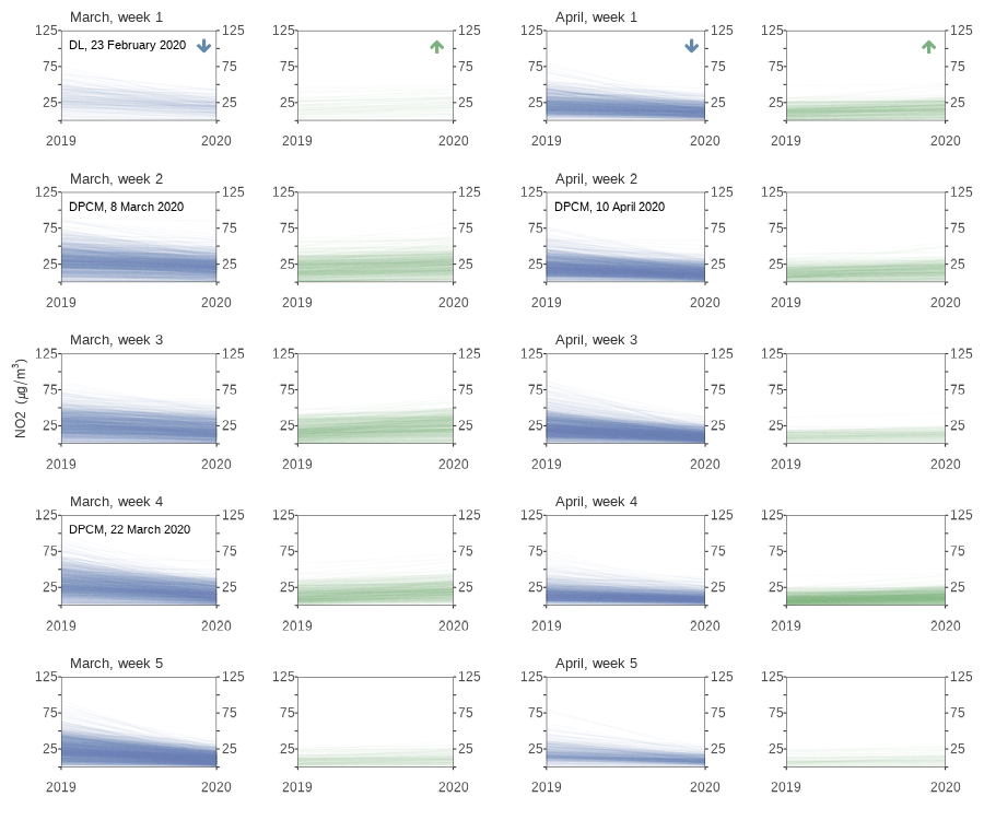
Figure 2: Aligned 2019-2020 daily NO₂ concentrations during the weeks of March and April. Each line represents a couple of aligned data of a monitoring site, distinguishing between decrements (blue lines) and increments (green lines) in NO₂ levels. The different government decrees and rules of the Italian lockdown are reported as text in the boxes. Each weekly plot depicts 1400 lines (200 monitoring sites times 7 days). Note that after the alignment process the first week of March contains just one day (Sunday, 200 lines) and the last week of April only two days (Monday and Thursday, 400 lines).

2.2 Spatial and spatio-temporal regressors

For each monitoring site, we retrieved its meteorological conditions and spatial characteristics for a total number of 13 independent explanatory variables (see Table 2), whose selection was driven by expert knowledge [Fioravanti et al., 2021].

To describe part of the spatial variation of the NO₂ daily differences, three geographical variables (constant in time) were considered: the linear distance from the the nearest major road, the altitude and the percentage of agricultural and arable lands. Yeganeh et al. [2018] found that traffic volume and congestion data for all of the individual roads can effectively improve the spatio-temporal modelling of NO₂ concentrations. Unfortunately, this information is not available for the whole investigated domain.

How weather affects NO₂ concentrations is assessed using 10 variables (such as total precipitation, wind speed, relative humidity, surface pressure) retrieved from the ERA5-Land dataset from the Copernicus Climate Data Store (https://climate.copernicus.eu/). ERA5-Land is a regridded version ($\sim$9 Km grid spacing) of the ERA5 climate reanalysis [Hersbach et al., 2020] of the European Centre for Medium-Range Weather Forecasts (ECMWF). The use of ERA5 data is documented, among others, by Chan et al. [2021] for investigating the effect of COVID-19 pandemic on NO₂ concentrations over Germany.

At this point it is important to stress that the meteorological variables enter the model as $2020-2019$ daily differences. More precisely, for the meteorological daily data we applied the same alignment procedure used for the NO₂ concentrations and described in Section 2.1.1. Afterwards, we calculated the daily differences which we used as model regressors, as explained in Section 3, where the details of the statistical model are given. It is worth to note that the inclusion in the model of the differenced meteorological variables alleviates potential multicollinearity problems and makes it possible to include in the same model regressors like temperature and surface pressure, which otherwise would be highly correlated.

Data Source		Description	Unit	Spatial Resolution
ERA5
		Minimum Planet Boundary Layer	Km	$\sim 9$ Km
		Maximum Planet Boundary Layer	Km
		Total Precipitation	mm
		Surface Pressure	hPa
		Average Temperature at 2 meters	∘C
		Wind Speed	m/s
		Previous day Wind Speed	m/s
		Relative Humidity	%
		Net Irradiance	$W/m^{2}$
		Diurnal Temperature Range	∘C
Global Multi-resolution Terrain Elevation Data
		Altitude	m	1 Km
OpenStreetMap
		Linear distance to the nearest primary road	m	1 km
Corine Land Cover
		Agricultural and arable lands	%	1 km

Table 2: Spatial and spatio-temporal predictors included in the model.

3 Bayesian spatio-temporal model

Consider a couple of NO₂ concentrations $y^{m}_{2019}(t,s_{i})$ and $y^{m}_{2020}(t,s_{i})$ temporally aligned according to the procedure described in Section 2.1.1, where $s_{i}$ denotes the location (with $i=1,\ldots,200$) and $t$ the day ($t=1,\ldots,T^{m}$) of month $m=1,2$ (where $m=1$ denotes March) of year 2019 and 2020, respectively.

As the objective of this study is to evaluate the change in NO₂ levels between 2019 and 2020, we first of all defined the daily differences of the log-transformed NO₂ concentrations:

$$\Delta^{m}(t,s_{i})=\log\left(y^{m}_{2020}(t,s_{i})\right)-\log\left(y^{m}_{2019}(t,s_{i})\right)=\log\left(\frac{y^{m}_{2020}(t,s_{i})}{y^{m}_{2019}(t,s_{i})}\right).$$ (1)

The logarithmic transformation is a common choice in air pollution analysis in order to reduce the typical positive skewness observed in concentrations distributions [Ott, 1990].

As the Italian lockdown fell almost at the end of the winter season, when usually the meteorological conditions favor the dispersion of the pollutants, a downward trend in NO₂ concentrations is expected across March and April. This could have a confounding effect when trying to isolate the impact of COVID-19 lockdown measures on air quality. In order to control for this long-term trend, we decided to model the daily differences separately for the two months (March and April).

The measurement equation is given by

$$\Delta(t,s_{i})=\mu(t,s_{i})+\epsilon(t,s_{i}),$$ (2)

where $\epsilon(t,s_{i})\sim N(0,\sigma^{2}_{\epsilon})$ is the Gaussian measurement error assumed to be independent in space and time. For the sake of simplicity in Equation (2) we omitted the index $m$ given that the model structure is the same for the considered months.

The mean level $\mu(t,s_{i})$ is then defined as the sum of fixed and random effects as follows:

$$\mu(t,s_{i})=\alpha_{0}+\alpha_{1}t+\gamma{I}^{S}_{t}+\bm{z}(s_{i})\bm{\beta}^{\prime}_{z}+\bm{\Delta}_{x}(t,s_{i})\bm{\beta}^{\prime}_{x}+v(s_{i})+u(t,s_{i}),$$ (3)

where $\alpha_{0}$ is the intercept and $\alpha_{1}t$ the linear temporal trend which should account for the short term variation across days in the month. The term $\bm{z}(s_{i})$ is the $p_{z}$-dimensional vector of the purely spatial regressors, while $\bm{\Delta}_{x}(s_{i},t)$ is the $p_{x}$-dimensional vector of the differences computed using the values of the meteorological regressors, as described in Section 2.2. We assume a linear effect for the spatial and spatio-temporal covariates by means of the parameters’ vector $\bm{\beta}_{z}$ and $\bm{\beta}_{x}$, respectively. In order to test whether or not there was a variation in the Sunday effect during the lockdown restrictions, we included also the dummy variable ${I}_{t}^{S}$ which is equal to 1 when $t$ is Sunday and zero otherwise. The corresponding coefficient $\gamma$ represents the additional expected change in the mean difference $\mu(t,s_{i})$ during Sunday. The term $v(s_{i})\sim N(0,\sigma^{2}_{v})$ represents a temporally and spatially uncorrelated Gaussian random effect which captures some of the small scale spatial variability. Finally, $u(t,s_{i})$ is the residual space-time correlation for which the following first order autoregressive dynamics was specified:

$$u(t,s_{i})=a\;u(t-1,s_{i})+\omega(t,s_{i}),$$

for $t=2,\ldots,T$ and $|a|<1$. The innovations $\omega(t,s_{i})$ have a zero-mean Gaussian distribution, are uncorrelated in time (i.e., $\text{Cov}\left(\omega(t,s_{i}),\omega(t^{\prime},s_{i})\right)=0$ if $t\neq t^{\prime}$) while being spatially correlated, i.e., $\text{Cov}\left(\omega(t,s_{i}),\omega(t,s_{j})\right)=\mathcal{C}(h)$, where $h$ is the Euclidean distance between site $i$ and $j$ and $\mathcal{C}(h)$ is the Matérn covariance function with variance $\sigma^{2}_{\omega}$ and range $\rho$. For more details about this separable spatio-temporal covariance structure see for example Cameletti et al. [2011, 2013].

3.1 Prior specification and model implementation

The model described in Section 3 is developed in the Bayesian framework and is fully specified once prior distributions are set.

Vague Gaussian priors were used for $\alpha_{0}$, $\alpha_{1}$ and for the elements of $\bm{\beta}_{z}$ and $\bm{\beta}_{x}$. For the remaining parameters Penalized Complexity (PC) priors [Simpson et al., 2017] were used. PC priors are a relatively new approach to specify weakly informative priors [Lemoine, 2019] in realistically complex statistical models with the twofold purpose of penalizing model complexity and avoiding overfitting.

For the standard deviation parameters (here $\sigma_{\epsilon}$ and $\sigma_{v}$) PC priors are generally defined as $\text{Prob}(\sigma>u_{\sigma})=\alpha_{\sigma}$, where $u_{\sigma}>0$ is a quantile of the prior and $0\leq\alpha_{\sigma}\leq 1$ is a probability value. In our analysis we set $u_{\sigma}=1$ and $\alpha_{\sigma}=0.1$ for both $\sigma_{\epsilon}$ and $\sigma_{v}$. This choice can be motivated considering that the total standard deviation of the observed daily differences of the log-transformed NO₂ concentrations is $\sim 0.5$ in each month, so it is very likely that the variance of each component is lower than 1.

The joint PC prior suggested in Fuglstad et al. [2019] was used for $\rho$ and $\sigma_{\omega}$. This can be specified through

$$\text{Prob}(\rho<u_{\rho})=\alpha_{\rho};\text{ }\text{Prob}(\sigma_{\omega}>u_{\sigma_{\omega}})=\alpha_{\sigma_{\omega}},$$

where we set $u_{\rho}=150$, $\alpha_{\rho}=0.8$, $u_{\sigma_{\omega}}=1$, $\alpha_{\sigma_{\omega}}=0.01$. Finally, for the autocorrelation parameter $a$ we used the PC prior proposed in Sørbye and Rue [2017]. This can be specified through $\text{Prob}(a>u_{a})=\alpha_{a}$, where we set $u_{a}=0.8$ and $\alpha_{a}=0.3$. All these choices reflect both previous findings [see e.g. Cameletti et al., 2013, Fioravanti et al., 2021] and restrictions to the possible values of $u_{a}$ and $\alpha_{a}$.

Inference was carried out by using the INLA-SPDE approach [Martino and Riebler, 2020, Lindgren and Rue, 2015], which has been proved to be computationally faster than the Markov chain Monte Carlo (MCMC) approach commonly used for Bayesian inference.

3.2 Prediction and posterior summary statistics

Once the model has been fitted to the observed data, we used Monte Carlo (MC) simulation to generate a large number of samples (say 1000) from the posterior predictive distribution of $\Delta(t,s)$ for any location $s$ in the study area and day $t$:

$$p\left(\Delta(t,s\right)\mid\mathcal{D})=\int p(\Delta(t,s)\mid\bm{\theta})p(\bm{\theta}\mid\mathcal{D}),$$ (4)

where $\bm{\theta}=\left(\alpha_{0},\alpha_{1},\gamma,\bm{\beta}_{x},\bm{\beta}_{z},a,\rho,u(t,s),\sigma^{2}_{\epsilon},\sigma^{2}_{v},\sigma^{2}_{\omega}\right)$ is the vector of all the model parameters, whose uncertainty is averaged out given all the observed data $\mathcal{D}$. For simplicity the generic sampled value will be denoted by $\hat{\Delta}(t,s)$.

To generate prediction maps, we used a raster grid with a spatial resolution of 1 km. For each pixel of this grid, corresponding to the generic location $s$, we simulated 1000 values $\hat{\Delta}(t,s)$ from Equation (4). While computing the predictions, we set the values of $\bm{\Delta}_{x}(s,t)$ equal to zero for each $s$ and $t$. This corresponds to assume that the meteorological conditions are equal in 2019 and 2020 for each location and time point.

We derived the posterior distribution of the relative change of NO₂ concentrations between 2019 and 2020 by using the following transformation:

$$\tilde{\Delta}(t,s)=\exp\left(\hat{\Delta}(t,s)\right)-1=\frac{\hat{y}_{2020}(t,s)}{\hat{y}_{2019}(t,s)}-1,$$ (5)

where $\tilde{\Delta}(t,s)$ takes negative (positive) values if lower (higher) NO₂ concentrations are expected in 2020 compared to 2019, and equal to zero in case of no change.

Finally, we averaged the 1000 MC samples from the daily distributions of $\tilde{\Delta}(t,s)$ at the week temporal resolution. The result is a collection of 1000 predicted raster maps for each week, from which it was possible to obtain the maps of the posterior mean and of the 2.5% and 97.5% quantiles. These latter two identify the bulk of the posterior distribution of each grid cell and were used to determine the 95% credible interval. When a credible interval does not include the zero, the corresponding relative change statistically differs from zero at the significance level of 0.05.

Finally, it is noteworthy to say that to take into account the weekly cycle of NO₂ concentrations, we generated both mean and quantile maps distinguishing between working days (Monday - Saturday) and weekends (Sunday).

3.3 Implementation and data availability

R software was used for the model implementation by means of the R-INLA package (https://www.r-inla.org). For the manipulation of the raster maps, we used the R raster package (https://cran.r-project.org/web/packages/raster/index.html) and the CDO software (https://code.mpimet.mpg.de/projects/cdo). Input data and part of the code used for this study are available through a dedicated GITHUB repository (https://github.com/progettopulvirus/A_spatiotemporal_analysis_of_NO2_concentrations).

4 Results and discussion

4.1 Model parameters

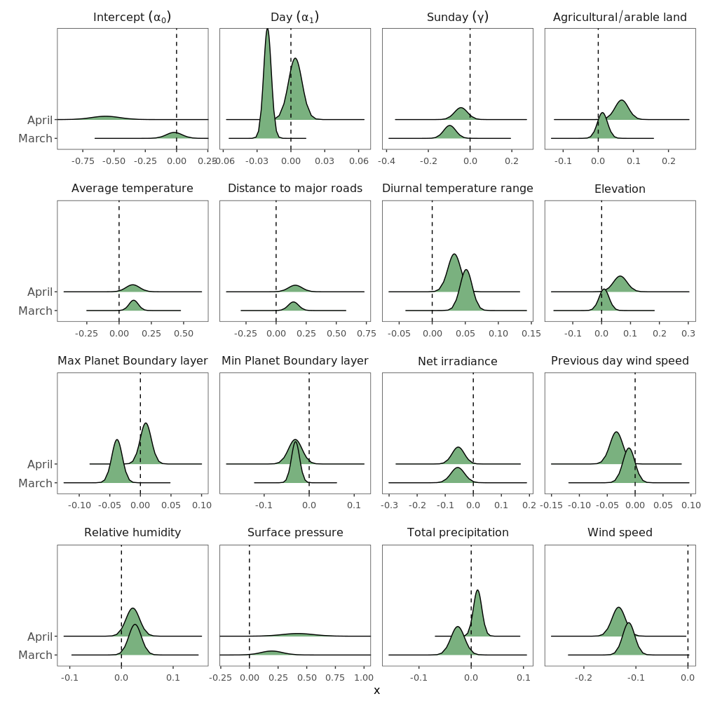
Figure 3: Posterior distribution of $\alpha_{0}$ (Intercept), $\alpha_{1}$ (Day), $\gamma$ (Sunday) and of the covariate coefficients $\bm{\beta}_{x}$ and $\bm{\beta}_{z}$. When the bulk of the posterior distribution lies far from zero it can be concluded that the corresponding parameter is significantly different from zero.

Figure 3 shows the monthly posterior distributions for the fixed effects’ coefficients ($\alpha_{0}$, $\alpha_{1}$, $\gamma$, $\bm{\beta}_{z}$ and $\bm{\beta}_{x}$). Generally speaking, we observe that a significant effect, invariant in sign across the months of March and April, characterizes most of the selected regressors. The shape of the posterior distributions is rather stable in the models for the two months, but some exceptions are apparent. The distribution of the linear trend coefficient $\alpha_{1}$ is narrower in March than in April, while the opposite happens for the posterior distribution of the intercept $\alpha_{0}$. This is in line with the large variability which characterizes the weekly prediction maps of April (see Section 4.3). Finally, the surface pressure coefficient exhibits two almost flat posterior distributions, but this result is not of easy interpretation.

A significant negative linear trend coefficient $\alpha_{1}$ was found in March, which suggests a decreasing trend for the daily differences of the log-transformed NO₂ concentrations in the month when the lockdown restrictions occurred. A significant negative effect was also found for the Sunday coefficient $\gamma$. We can interpret this result saying that a weekly cycle persists even when we consider the difference of the log-transformed NO₂ concentrations. Surprisingly, neither the linear trend nor the Sunday dummy variable coefficients are significant in April.

With regards to the meteorological parameters, we distinguish those with a positive significant effect (the diurnal temperature range, the average temperature at 2 meters, the relative humidity and surface pressure) and those with a negative significant effect (the min and max planet boundary layer, the net irradiance, the wind speed and the total precipitation). Conversely, all the spatial regressors (elevation, % of agricultural/arable land and distance to major roads) show a positive posterior mean. This could suggest that far from the urbanized centers and the road network the level of the NO₂ daily concentrations in 2020 tends to be equal or greater than the ones in 2019.

Table 3 provides the posterior summary statistics for the remaining model parameters. We observe that the posterior mean of the AR(1) autocorrelation coefficient $a$, the spatial range $\rho$ and the standard deviation $\sigma_{v}$ have a larger posterior mean in April than in March.

	$a$	$\rho$	$\sigma_{v}$	$\sigma_{\epsilon}$	$\sigma_{\omega}$
March	0.64 (0.023)	74 (4.0)	0.16 (0.011)	0.21 (0.004)	0.37 (0.013)
April	0.80 (0.021)	97 (5.5)	0.22 (0.015)	0.22 (0.003)	0.42 (0.021)

Table 3: Posterior mean and standard deviation (in parentheses) of the parameters in the models for March and April. $a$: AR(1) coefficient; $\rho$ and $\sigma_{\omega}$: range (in km) and standard deviation of the Matérn spatial covariance function; $\sigma_{v}$: standard deviation of the small scale spatial random effect; $\sigma_{\epsilon}$: standard deviation of the Gaussian measurement error.

4.2 Model validation

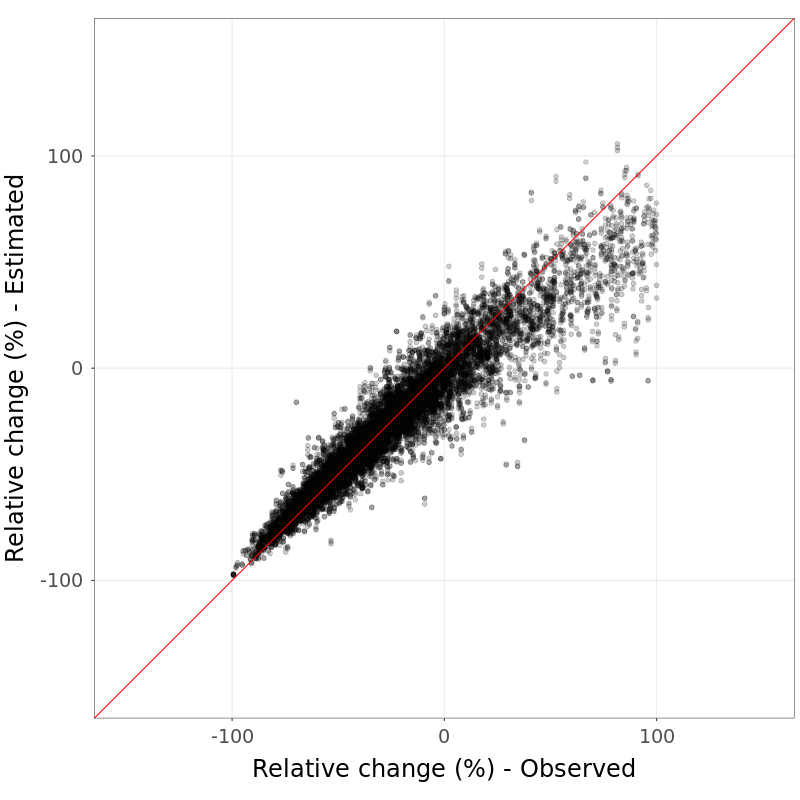
(a) Training stage - March

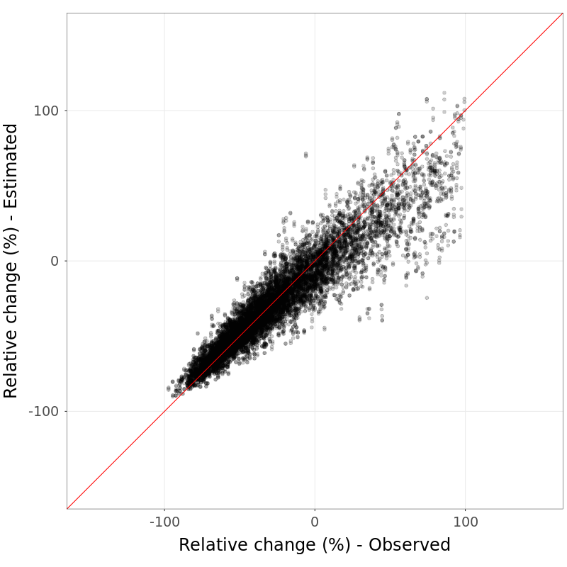
(b) Training stage - April

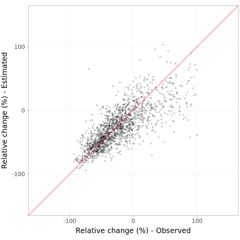
(c) Validation stage - March

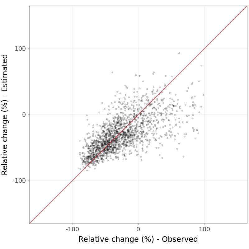
(d) Validation stage - April

Figure 4: Agreement between modelled and measured $\text{NO}_{2}$ relative change ($\tilde{\Delta}(t,s)\%$) in the training (top) and validation stage (bottom). The solid red line is the 1:1 line as a reference.

For validation purposes, we stratified the input monitoring sites according to their type classification (urban, suburban and rural stations). Within each of these groups, we sampled 10% of the stations in order to define a validation dataset. The remainder of the stations (training dataset) was used to fit the model and the fitted model was used to predict the daily differences of the log-transformed NO₂ concentrations (see Equation (1)) on the validation dataset. Both the sampling and the estimation process were repeated three times for each month. Comparing predicted and observed values allows to investigate how the model performes on unseen data, specifically if the model generalizes well or suffers from overfitting/underfitting.

Plots and summary statistics are shown as percentage relative changes $\tilde{\Delta}(t,s)\%$ (see Equation (5)) for ease of interpretation of the validation results. The scatterplots in Figure 4 shows the distribution of the fitted values versus the observed values. The points spread uniformly along the diagonal line, showing good agreement between observed and modelled data both in the training and validation stage. As expected, modelled relative change for the validation stage shows greater variability than in the training stage. Also the Pearson correlation coefficients support the good model performance with a value of 0.9 for the training stage and of $\sim 0.7$ for the validation stage. Finally, the Root Mean Squared Error is $\sim 10\%$ and $\sim 20\%$ for the training and validation stage, respectively.

4.3 NO₂ 2019/2020 relative change maps

Using the predictors described in Section 2.2 as individual raster files, the procedure described in Section 3.2 was implemented to obtain maps of the relative change of NO₂ concentrations between 2019 and 2020, separately for the weeks of March and April.

The maps in Figure 5 and 6 show the spatial pattern of the 2019/2020 relative change of NO₂ concentration in the north/centre of Italy for March and April, respectively. These maps refer to the weekly averaged estimates obtained from working days (Monday - Saturday), while the weekly Sunday estimates are available in the Annex (see Section 6). This distinction between working days and Sunday maps reflects our choice of including a dummy regressor for the Sunday effect in the model and its statistical significance observed in March. For visualization purposes, we limited the data range between -100% and +100% and used a scientifically derived color map [Crameri et al., 2020]. Furthermore, the islands from the Tuscan Archipelago are not displayed and Liguria region, where no daily NO₂ concentrations were available, is represented with a white background.

It is worthwhile to stress that the maps presented in this section must be intended as meteorology-normalized maps. This means that they were generated assuming that, in each cell of the raster grid, the daily meteorological conditions are exactly the same in 2019 and 2020. Mathematically, this assumption is equivalent to setting to zero all the meteorological terms in our spatio-temporal model (see Section 3.2).

Figure 5 and 6 reveal a substantial decrease in NO₂ concentrations during March and April 2020 as compared to 2019. A statistically significant reduction persists during the third and fourth working weeks of March across the whole study area: we quantified the interquartile range of the corresponding relative changes distribution to be between -40% and -20%, as shown in the boxplot in the left panel of Fig. 7. Notably, the third and fourth week of March correspond to the stringent phase of the COVID-19 lockdown. The barplots of Figure 8 indicate that Lombardy, Veneto, Friuli Venezia Giulia and Emilia Romagna are the regions where significant reductions in the NO₂ concentrations mostly occurred. Conversely, Tuscany region in the centre and the mountainous regions of Valle d’Aosta and the Autonomus Provinces of Bolzano and Trento are those where most of the estimated changes have no statistical significance.

In April the predicted surfaces show more spatial variability than in March and all the weekly distributions of the relative changes (right panel of Fig. 7) exhibit positive increments up to 100%. These results suggest that the NO₂ concentrations began to recover in April. Surprisingly, the fourth week of April is overwhelmed by a significant increment in the agricultural/arable area of the Po Valley (median increment around 10%), while a spatially homogeneous decrease, like the one observed in the second half of March, occurs only during the third week of the month (interquartile range between -40% and -20%). Note that during most of April 2020 the lockdown restrictions were the same of the third and fourth week of March. Looking at the maps of Figure 6, it is apparent that the urbanized belt of the Po valley shows a persistent significant negative change during almost all the weeks of April. This is confirmed by the barplots of Figure 8. Despite this variegated situation, the weekly distributions of the relative changes still are dominated by negative values with median values around -30%, with the exception of the fourth week.

Generally speaking, the estimates from the Sunday maps (see Section 6) are consistent with those obtained for working days. The most pronounced decline of the NO₂ concentrations occurs during the last two Sundays of March: we find a -40% median relative change in 2020 as compared to the same period in 2019. The same drop in the NO₂ concentrations is quantified for the second week of April (when Easter 2020 occured).

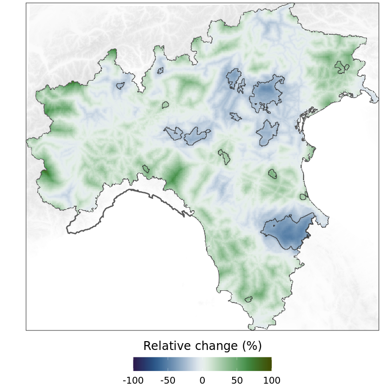
(a) March - First week

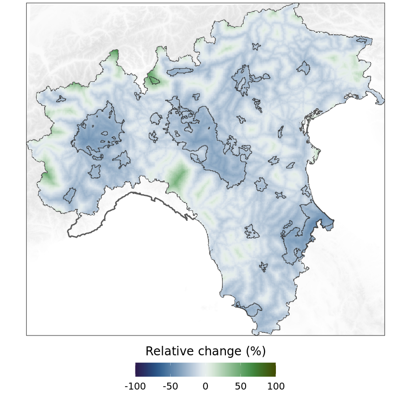
(b) March - Second week

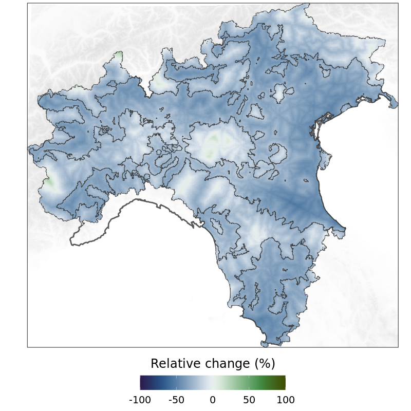
(c) March - Third week

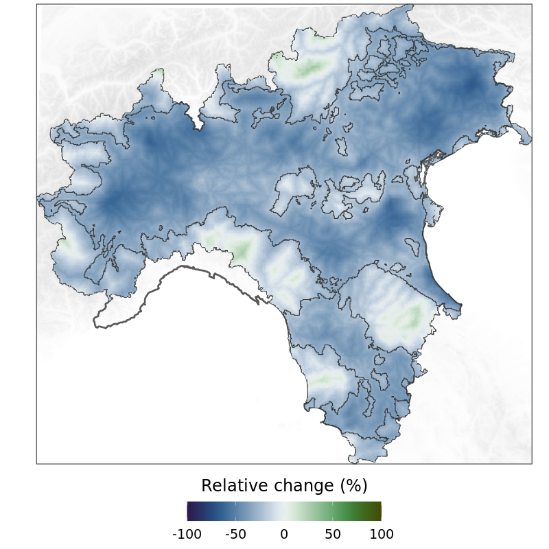
(d) March - Fourth week

Figure 5: Weekly maps of the NO₂ 2019/2020 relative change (%) for the working days (Monday - Saturday). Contour lines mark those areas where the relative change is statistically significant at the significance level of 0.05.

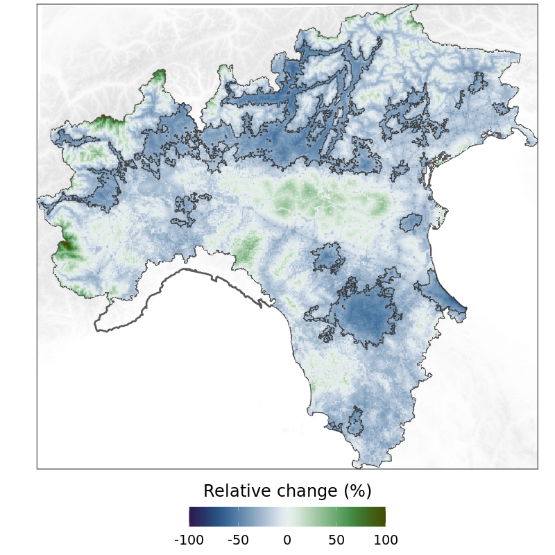
(a) April - First week

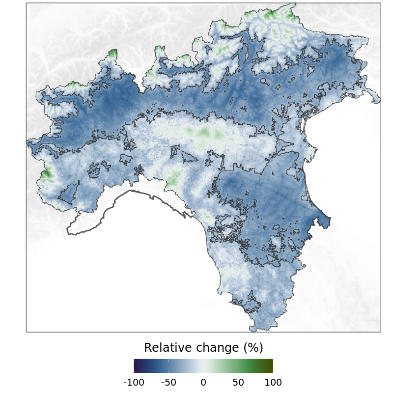
(b) April - Second week

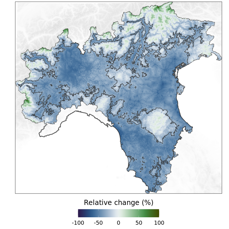
(c) April - Third week

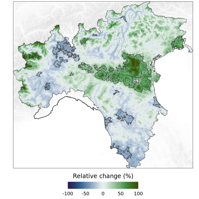
(d) April - Fourth week

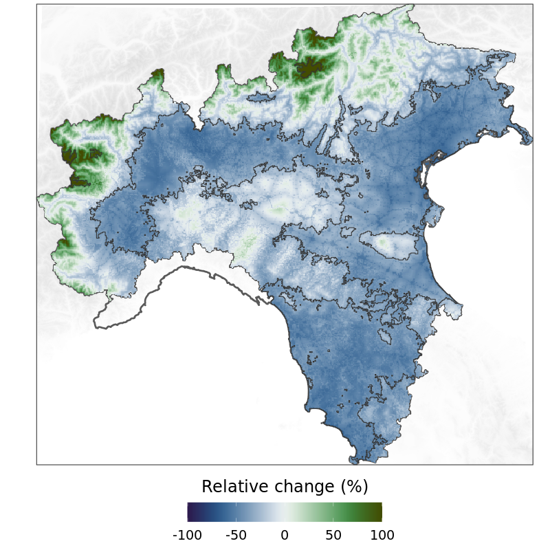
(e) April - Fifth week

Figure 6: Weekly maps of the NO₂ 2019/2020 relative change (%) for the working days (Monday - Saturday). Contour lines mark those areas where the relative change is statistically significant at the significance level of 0.05.

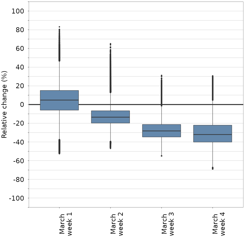
(a) March

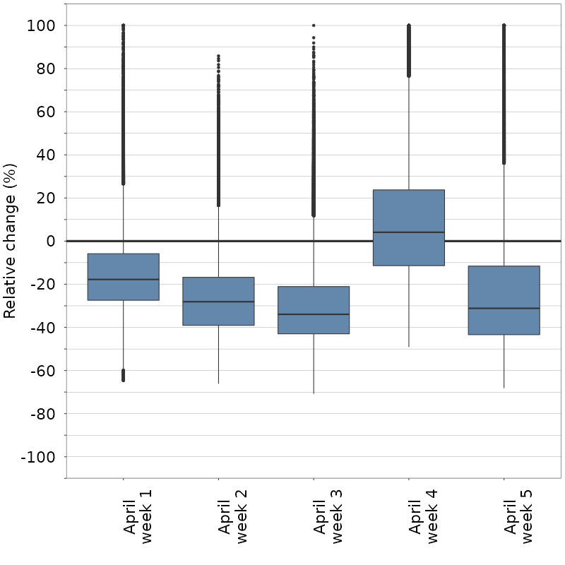
(b) April

Figure 7: Distribution of the NO₂ 2019/2020 relative change (%) for the working days (Monday - Saturday) maps.

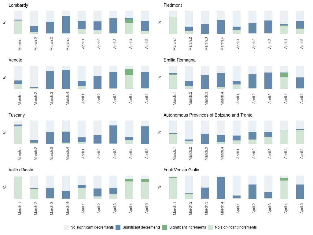
Figure 8: Percentage of cells in the prediction maps for working days (Monday - Saturday) with positive (green color scale) and negative (blue color scale) 2019/2020 relative changes. Darker colors are used for significant variations.

5 Conclusions

Capturing the spatio-temporal variation in pollutant concentrations is of keen interest for the air pollution management’s community. One of the reasons is that the effectiveness of environmental policies or interventions, or even exceptional events as the COVID-19 lockdown, must be evaluated across the whole study domain, in order to understand if the change is homogeneous in space or peculiar spatial patterns occur. This analysis is made even more difficult by the fact that air pollution dynamics strongly depends on weather conditions; thus, it is necessary to disentangle the effect of the adopted intervention by controlling for the known confounding factors. Chemical transport model can be used for this purpose. They can assess, with a very detailed spatial and temporal resolution, variations due to changes in the emission burden arising from interventions, like the implementation of air quality plans. However, some drawbacks exist: CTMs need very detailed input data (e.g., emission inventories, meteorology data), are complex to be run and rely on advanced IT infrastructure for their simulations. More importantly, they do not provide an estimate of the uncertainty of the final predictions which are also strongly dependent on the initial and boundary conditions. Moving to statistical models, it is straightforward to deal with uncertainty and spatio-temporal correlation structures, while keeping the computational costs at a reasonable level (especially if computationally efficient estimation methods, like the INLA-SPDE approach, are used).

In this paper we propose the use of a statistical Bayesian spatio-temporal model as a novel tool for assessing - in time but more importantly in space - the effectiveness of air quality policy interventions. As a case study, we focused on how the COVID-19 lockdown affected air pollution levels in the north/centre of Italy, by means of the 2019/2020 NO₂ concentrations relative change, the main output of our modeling strategy. Even if our proposal does not explicitly simulate physical and chemical reactions in the atmosphere (like CTMs do), it has two key advantages: it is parsimonious in terms of data needs and, possibly more important, it naturally manages the uncertainty associated to the parameters and map outputs. The proposed method, applied to a real-world experiment, demonstrated its capability to provide a reliable picture of the temporal and spatial patterns of the NO₂ variations (compared to 2019), while accounting for the effect of meteorology.

In this study, the spatio-temporal variation of the NO₂ concentrations in March and April 2020, as compared with the same period in 2019, is illustrated through meteorology-normalized spatially continuous maps at weekly intervals, both for working days (Monday - Saturday) and weekends (Sunday). Our results show that during March and April 2020 the study domain was generally characterized by negative relative changes in the NO₂ concentrations with median values around -25%. Such estimate seems to be reasonably consistent with previous findings about NO₂ levels during the lockdown in Europe. However, the message from our output maps is richer than what a simple number can describe. First, a visual inspection of the maps shows that statistically significant reductions mainly occurred in the urban areas of the Po valley and Tuscany, while not significant variations persisted over the mountainous regions of Valle d’Aosta and the Autonoumous Provinces of Bolzano and Trento. Second, and more interestingly, our weekly analysis of NO₂ highlight that in March 2020 such reduction was synchronous with the lockdown measures adopted, while in April 2020 the concentrations, as compared to 2019, started to recover in some parts of the investigated area. To the authors of this study, this result comes not unexpected as it reflects the behaviour of the input data seen in the parallel plot of Figure 2. At the same time, it comes as a surprise that none of the statistical studies we examined documented an increase in the NO₂ concentrations in April in the studied Italian domain. However, we are aware that previous findings are based on different models, data, and methodologies, so our results are not directly comparable, especially if we consider that all these studies do not provide continuous maps as an output.

It is worthwhile to observe that our modeling approach does not allow us to draw causal inference conclusions. However, given that the maps account for the weather effect, we can conclude that the reductions we observe across regions and weeks can be attributed to a factor different from the meteorology. Given that they occur in the same period of the restrictive measures, it is likely that the COVID-19 lockdown had an effect in the reduction of air pollution. Nevertheless, we can not exclude that other factors, not considered in the model, could have ad an active role in the dynamics of NO₂.

The model described in this paper takes inspiration from the model introduced in Fioravanti et al. [2021] for the spatio-temporal assessment of the daily log-transformed PM₁₀ concentrations in Italy. As here our objective was to describe the relative changes across the two considered years (2019 vs 2020), in this study the target variable is the daily differences of the log-transformed NO₂ concentrations. As far as we know this modeling strategy has never been used before in the context of spatio-temporal models for intervention analysis. Other approaches could have been adopted, still in the context of spatio-temporal modeling. For example, the same problem could have also been tackled by, first, jointly modeling the 2019 and 2020 NO₂ concentrations and then computing the differences between the daily gridded predictions. However, this alternative solution has two important shortcomings: 1) it is not consistent with the AR(1) assumption, as our observations are not consecutive in time but are one year apart (March-April 2019 and 2020); 2) it is more time consuming as the size of the input dataset would be as twice as the size of the input dataset when daily differences are considered. Furthermore, the use of daily differences alleviates multicollinearity among regressors and allows to include more parameters in the regression equation. For this reason we believe that the spatio-temporal model we propose represents a valid solution to analyze pollutant concentrations measured by a network of monitoring stations before and after a given event of interest (e.g., the lockdown intervention). Interestingly, our model allows a straightforward spatial assessment of NO₂ variations through high-resolution estimates, since the posterior predictive distributions of NO₂ differences can virtually be derived for every pixel within the study domain. This is of keen interest for policy makers involved in intervention analysis or epidemiologist assessing population exposure change and gradients, since the assessment at urban hot spot, the between-city variability as well as the comparison among rural and urban context can be achieved at the finest resolution, with a reasonable computational effort. In this regard, our approach could be usefully replicated whenever the effects of an intervention aimed to reduce the pollutant emissions at local or regional scale have to be assessed. Last but not least, the proposed model is simple and can be easily extended to a larger spatial domain. This means that it could be also applied to other pollutants or, more generally, spatio-temporal phenomenon which are continuous in space and for which it is interesting to evaluate the change in consecutive years.

6 Appendix

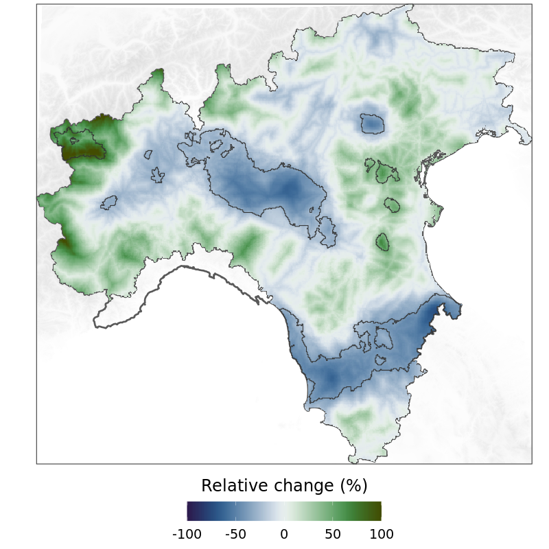
(a) March - First week

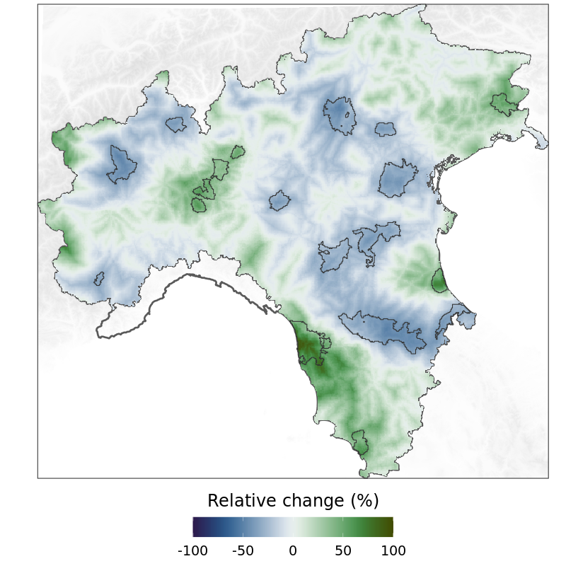
(b) March - Second week

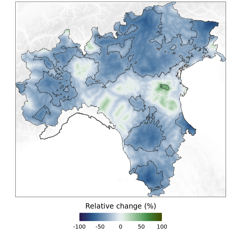
(c) March - Third week

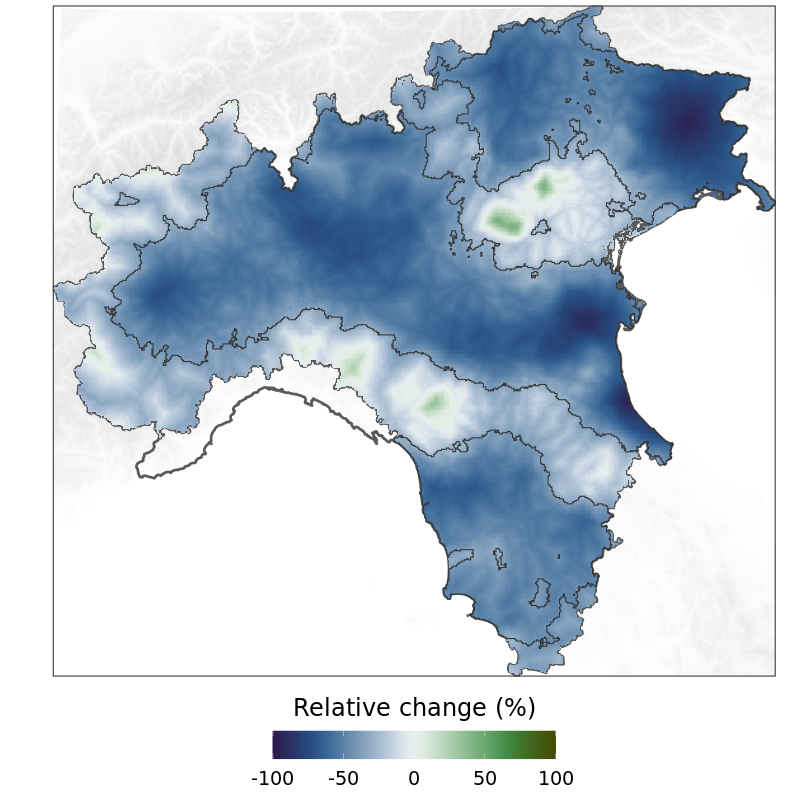
(d) March - Fourth week

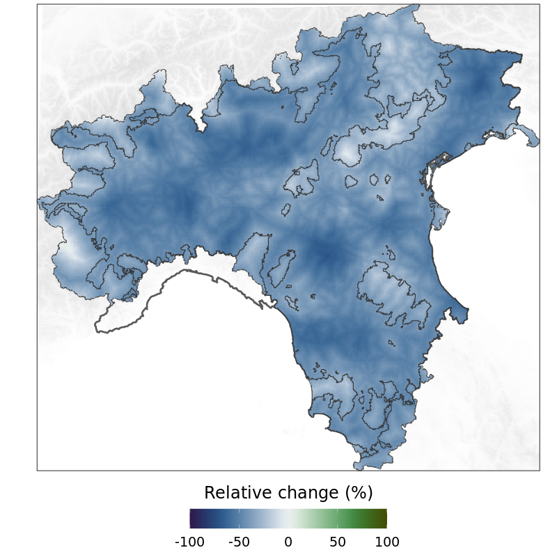
(e) March - Fifth week

Figure 9: Weekly maps of the NO₂ 2019/2020 relative change (Sunday). Contour lines mark those areas where the relative change is statistically significant at the significance level of 0.05.

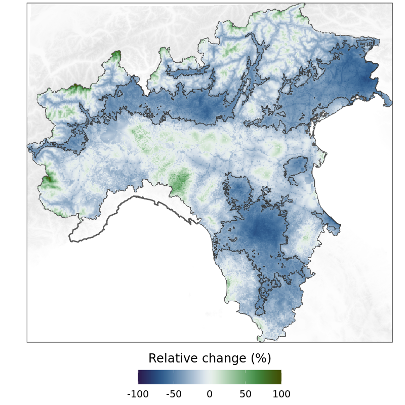
(a) April - First week

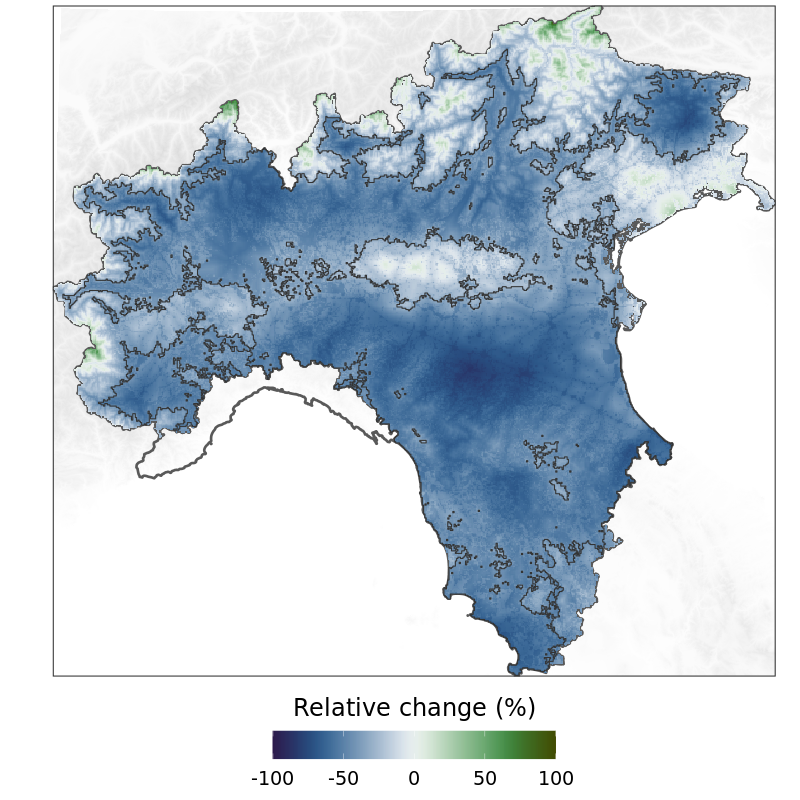
(b) April - Second week

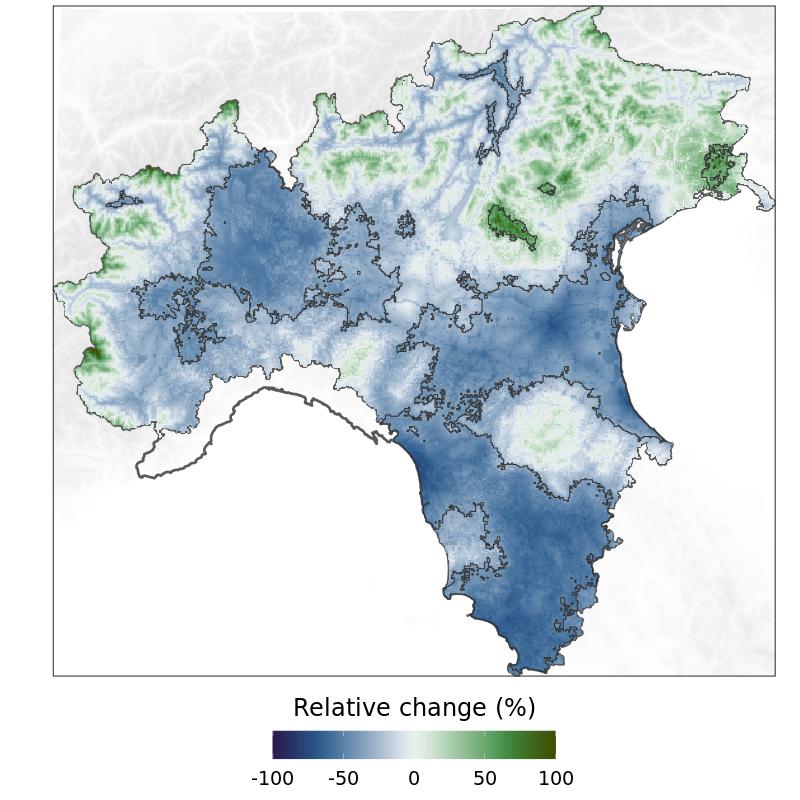
(c) April - Third week

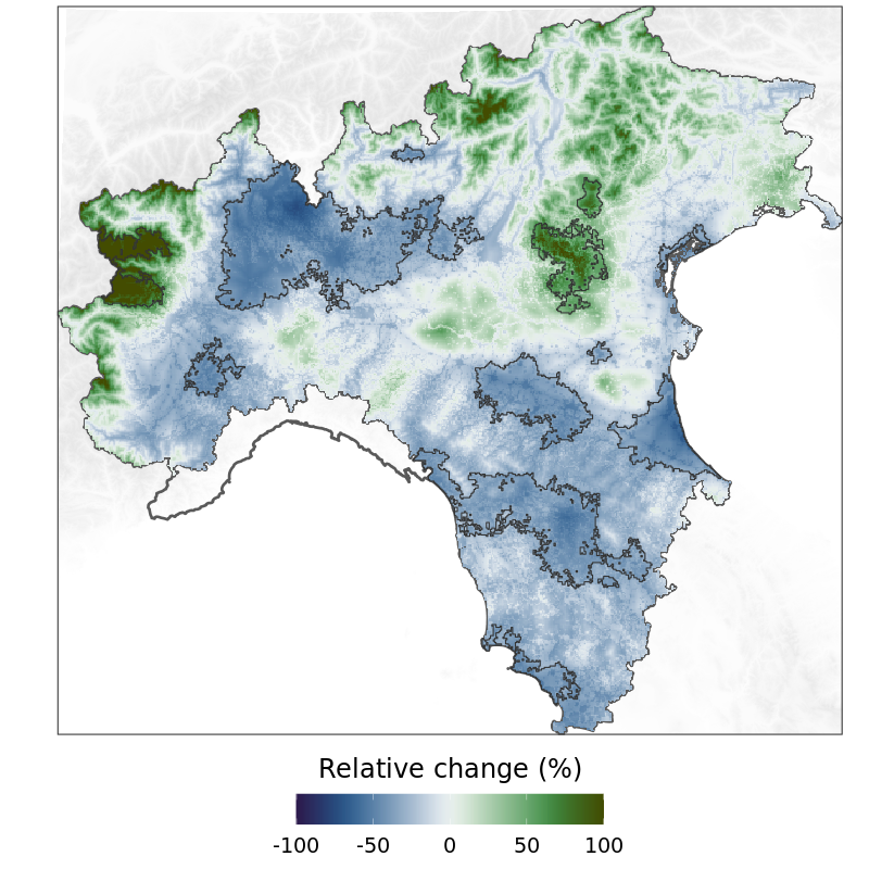
(d) April - Fourth week

Figure 10: Weekly maps of the NO₂ 2019/2020 relative change (Sunday). Contour lines mark those areas where the relative change is statistically significant at the significance level of 0.05.

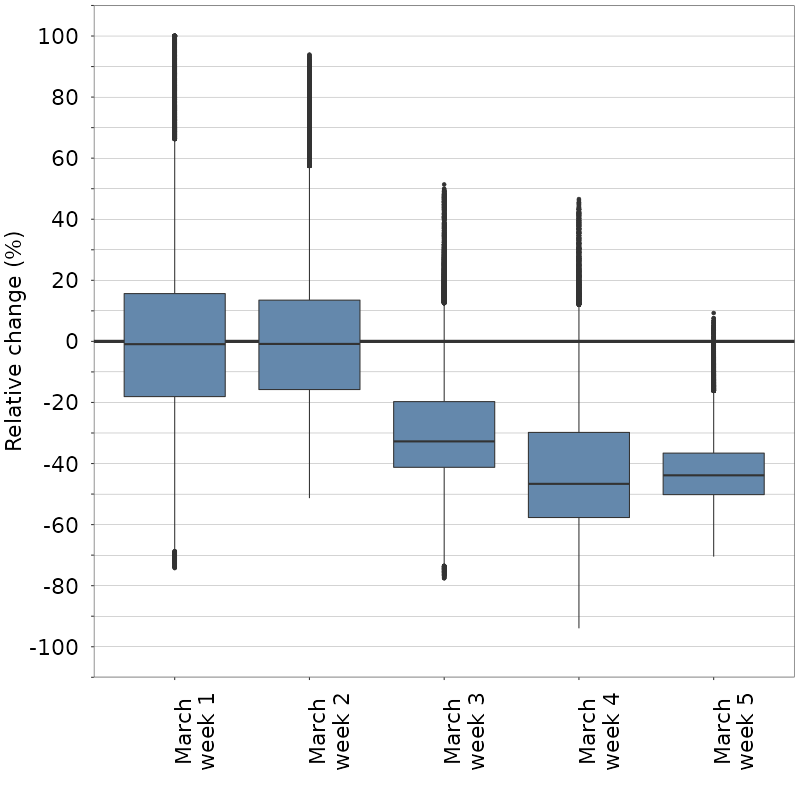
(a) March

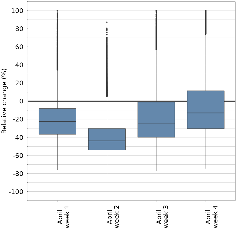
(b) April

Figure 11: Distribution of the estimated NO₂ 2019/2020 relative change (%) for the Sunday maps.

7 Acknowledgments

This research has been carried out within the framework of the PULVIRUS partnership agreement between ENEA, ISPRA, SNPA and ISS.

We wish to thank for their helpful contribution to the air quality and meteorological data pre-processing Raffaele Morelli, Walter Perconti and Arianna Trentini. In addition, we wish to thank all the Regional Environmental Protection Agencies (ARPA Valle d’Aosta, ARPA Piemonte, ARPA Lombardia, ARPA Veneto, APPA Bolzano, APPA Trento, ARPA Friuli, ARPAE Emilia Romagna, ARPA Toscana) that manage the air quality networks and provide fully validated NO₂ hourly data.

This research did not receive any specific grant from funding agencies in the public, commercial, or not-for-profit sectors.

Author contributions

Guido Fioravanti, Michela Cameletti and Sara Martino conceived the presented model. Guido Fioravanti prepared the data with the support of Giorgio Cattani and performed computations. Michela Cameletti took the lead in writing the manuscript. Sara Martino verified the analytical methods. Giorgio Cattani and Enrico Pisoni contributed to the interpretation of the results. All authors discussed the results and contributed to the final version of the manuscript.

Financial disclosure

None reported.

Conflict of interest

The authors declare no potential conflict of interests.

References

- Bao and Zhang [2020] Rui Bao and Acheng Zhang. Does lockdown reduce air pollution? Evidence from 44 cities in northern China. Science of The Total Environment, 731:139052, 2020. ISSN 0048-9697. doi: https://doi.org/10.1016/j.scitotenv.2020.139052. URL https://www.sciencedirect.com/science/article/pii/S0048969720325699.
- Bar et al. [2021] Somnath Bar, Bikash Ranjan Parida, Shyama Prasad Mandal, Arvind Chandra Pandey, Navneet Kumar, and Bibhudatta Mishra. Impacts of partial to complete COVID-19 lockdown on NO2 and PM2.5 levels in major urban cities of Europe and USA. Cities, 117:103308, 2021. ISSN 0264-2751. doi: https://doi.org/10.1016/j.cities.2021.103308. URL https://www.sciencedirect.com/science/article/pii/S0264275121002080.
- Barré et al. [2020] J. Barré, H. Petetin, A. Colette, M. Guevara, V. H. Peuch, L. Rouil, R. Engelen, A. Inness, J. Flemming, C. Pérez García-Pando, D. Bowdalo, F. Meleux, C. Geels, J. H. Christensen, M. Gauss, A. Benedictow, S. Tsyro, E. Friese, J. Struzewska, J. W. Kaminski, J. Douros, R. Timmermans, L. Robertson, M. Adani, O. Jorba, M. Joly, and R. Kouznetsov. Estimating lockdown induced European NO2 changes. Atmospheric Chemistry and Physics Discussions, 2020:1–28, 2020. doi: 10.5194/acp-2020-995. URL https://acp.copernicus.org/preprints/acp-2020-995/.
- Bassani et al. [2021] Cristiana Bassani, Francesca Vichi, Giulio Esposito, Mauro Montagnoli, Marco Giusto, and Antonietta Ianniello. Nitrogen dioxide reductions from satellite and surface observations during COVID-19 mitigation in Rome (Italy). Environmental Science and Pollution Research, 2021.
- Bauwens et al. [2020] M. Bauwens, S. Compernolle, T. Stavrakou, J. F. Müller, J. van Gent, H. Eskes, P. F. Levelt, R. van der A, J. P. Veefkind, J. Vlietinck, H. Yu, and C. Zehner. Impact of Coronavirus Outbreak on NO2 Pollution Assessed Using TROPOMI and OMI Observations. Geophysical Research Letters, 47(11), 2020.
- Beloconi et al. [2021] Anton Beloconi, Nicole M. Probst-Hensch, and Penelope Vounatsou. Spatio-temporal modelling of changes in air pollution exposure associated to the COVID-19 lockdown measures across Europe. Science of The Total Environment, 787:147607, 2021. ISSN 0048-9697. doi: https://doi.org/10.1016/j.scitotenv.2021.147607. URL https://www.sciencedirect.com/science/article/pii/S0048969721026784.
- Burns et al. [2020] J. Burns, H. Boogaard, S. Polus, L.M. Pfadenhauer, A.C. Rohwer, A.M. van Erp, R. Turley, and E.A. Rehfuess. Interventions to reduce ambient air pollution and their effects on health: An abridged cochrane systematic review. Environment International, 135:105400, 2020. ISSN 0160-4120. doi: https://doi.org/10.1016/j.envint.2019.105400.
- Cameletti [2020] Michela Cameletti. The Effect of Corona Virus Lockdown on Air Pollution: Evidence from the City of Brescia in Lombardia Region (Italy). Atmospheric Environment, 239:117794, 2020. ISSN 1352-2310. doi: https://doi.org/10.1016/j.atmosenv.2020.117794. URL https://www.sciencedirect.com/science/article/pii/S1352231020305288.
- Cameletti et al. [2011] Michela Cameletti, Rosaria Ignaccolo, and Stefano Bande. Comparing spatio-temporal models for particulate matter in Piemonte. Environmetrics, 22(8):985–996, 2011. doi: https://doi.org/10.1002/env.1139. URL https://onlinelibrary.wiley.com/doi/abs/10.1002/env.1139.
- Cameletti et al. [2013] Michela Cameletti, Finn Lindgren, Daniel Simpson, and Håvard Rue. Spatio-temporal modeling of particulate matter concentration through the SPDE approach. AStA Advances in Statistical Analysis, 97(2):109–131, 2013.
- Carlos et al. [2020] Ordóñez Carlos, Garrido-Perez Jose M., and García-Herrera Ricardo. Early spring near-surface ozone in Europe during the COVID-19 shutdown: Meteorological effects outweigh emission changes. Science of The Total Environment, 747:141322, 2020. ISSN 0048-9697. doi: https://doi.org/10.1016/j.scitotenv.2020.141322. URL https://www.sciencedirect.com/science/article/pii/S0048969720348518.
- CEN-TC 264 [2012] Air quality CEN-TC 264. European standard en 14211:2012 ambient air quality — standard method for the measurement of the concentration of nitrogen dioxide and nitrogen monoxide by chemiluminescence. Technical report, European Union, 2012.
- Cersosimo et al. [2020] Angela Cersosimo, Carmine Serio, and Guido Masiello. TROPOMI NO2 Tropospheric Column Data: Regridding to 1 km Grid-Resolution and Assessment of their Consistency with In Situ Surface Observations. Remote Sensing, 12(14), 2020. ISSN 2072-4292. doi: 10.3390/rs12142212. URL https://www.mdpi.com/2072-4292/12/14/2212.
- Chan et al. [2021] Ka Lok Chan, Ehsan Khorsandi, Song Liu, Frank Baier, and Pieter Valks. Estimation of Surface NO2 Concentrations over Germany from TROPOMI Satellite Observations Using a Machine Learning Method. Remote Sensing, 13(5), 2021. ISSN 2072-4292. doi: 10.3390/rs13050969. URL https://www.mdpi.com/2072-4292/13/5/969.
- Crameri et al. [2020] F. Crameri, G.E. Shephard, and P.J. Heron. The misuse of colour in science communication. Nat Commun, 2020. doi: 10.1038/s41467-020-19160-7.
- Dacre et al. [2020] H. F. Dacre, A. H. Mortimer, and L. S. Neal. How have surface NO2 concentrations changed as a result of the UK’s COVID-19 travel restrictions? Environmental Research Letters, 15(10):104089, 2020. doi: 10.1088/1748-9326/abb6a2. URL https://doi.org/10.1088/1748-9326/abb6a2.
- Diémoz et al. [2021] Henri Diémoz, Tiziana Magri, Giordano Pession, Claudia Tarricone, Ivan Karl Friedrich Tombolato, Gabriele Fasano, and Manuela Zublena. Air Quality in the Italian Northwestern Alps during Year 2020: Assessment of the COVID-19 Lockdown Effect from Multi-Technique Observations and Models. Atmosphere, 12(8), 2021. ISSN 2073-4433. doi: 10.3390/atmos12081006. URL https://www.mdpi.com/2073-4433/12/8/1006.
- Donzelli et al. [2020] Gabriele Donzelli, Lorenzo Cioni, Mariagrazia Cancellieri, Agustin Llopis Morales, and Maria M. Morales Suárez-Varela. The Effect of the Covid-19 Lockdown on Air Quality in Three Italian Medium-Sized Cities. Atmosphere, 11(10), 2020. doi: 10.3390/atmos11101118. URL https://www.mdpi.com/2073-4433/11/10/1118.
- Dutta et al. [2021] Venkatesh Dutta, Saroj Kumar, and Divya Dubey. Recent advances in satellite mapping of global air quality: evidences during COVID-19 pandemic. Environmental Sustainability, 2021.
- EEA [2020] EEA. Air quality in Europe - 2020 Report. Technical report, European Environmental Agency (EEA), 2020. https://www.eea.europa.eu/publications/air-quality-in-europe-2020-report.
- Fassò [2013] Alessandro Fassò. Statistical assessment of air quality interventions. Stochastic Environmental Research and Risk Assessment, 27(7):1651–1660, 2013.
- Finazzi et al. [2013] Francesco Finazzi, E. Marian Scott, and Alessandro Fassò. A model-based framework for air quality indices and population risk evaluation, with an application to the analysis of scottish air quality data. Journal of the Royal Statistical Society: Series C (Applied Statistics), 62(2):287–308, 2013. doi: https://doi.org/10.1111/rssc.12001.
- Fioravanti et al. [2021] Guido Fioravanti, Sara Martino, Michela Cameletti, and Giorgio Cattani. Spatio-temporal modelling of PM10 daily concentrations in Italy using the SPDE approach. Atmospheric Environment, 248:118192, 2021. doi: https://doi.org/10.1016/j.atmosenv.2021.118192.
- Font and Fuller [2016] Anna Font and Gary W. Fuller. Did policies to abate atmospheric emissions from traffic have a positive effect in London? Environmental Pollution, 218:463–474, 2016. ISSN 0269-7491. doi: https://doi.org/10.1016/j.envpol.2016.07.026.
- Fuglstad et al. [2019] G.-A. Fuglstad, D. P. Simpson, F. Lindgren, and H. Rue. Constructing priors that penalize the complexity of Gaussian Random Fields. J. Am. Stat. Assoc., 114(525):445–452, 2019.
- Gkatzelis et al. [2021] Georgios I. Gkatzelis, Jessica B. Gilman, Steven S. Brown, Henk Eskes, A. Rita Gomes, Anne C. Lange, Brian C. McDonald, Jeff Peischl, Andreas Petzold, Chelsea R. Thompson, and Astrid Kiendler-Scharr. The global impacts of COVID-19 lockdowns on urban air pollution: A critical review and recommendations. Elementa: Science of the Anthropocene, 9(1), 2021. doi: 10.1525/elementa.2021.00176.
- Granella et al. [2021] Francesco Granella, Lara Aleluia Reis, Valentina Bosetti, and Massimo Tavoni. COVID-19 lockdown only partially alleviates health impacts of air pollution in Northern Italy. Environmental Research Letters, 16(3):035012, 2021. doi: 10.1088/1748-9326/abd3d2. URL https://doi.org/10.1088/1748-9326/abd3d2.
- Grange et al. [2021] S. K. Grange, J. D. Lee, W. S. Drysdale, A. C. Lewis, C. Hueglin, L. Emmenegger, and D. C. Carslaw. Covid-19 lockdowns highlight a risk of increasing ozone pollution in european urban areas. Atmospheric Chemistry and Physics, 21(5):4169–4185, 2021. doi: 10.5194/acp-21-4169-2021. URL https://acp.copernicus.org/articles/21/4169/2021/.
- Grange and Carslaw [2019] Stuart K. Grange and David C. Carslaw. Using meteorological normalisation to detect interventions in air quality time series. Science of The Total Environment, 653:578–588, 2019. ISSN 0048-9697. doi: https://doi.org/10.1016/j.scitotenv.2018.10.344.
- Han et al. [2021] Yang Han, Jacqueline CK Lam, Victor OK Li, and David Reiner. A Bayesian LSTM model to evaluate the effects of air pollution control regulations in Beijing, China. Environmental Science and Policy, 115:26–34, 2021. ISSN 1462-9011. doi: https://doi.org/10.1016/j.envsci.2020.10.004.
- He et al. [2020] Guojun He, Yuhang Pan, and Takanao Tanaka. The short-term impacts of COVID-19 lockdown on urban air pollution in China. Nature Sustainability, 3(12):1005–1011, 2020.
- Hersbach et al. [2020] H. Hersbach, B. Bell, P. Berrisford, S. Hirahara, A. Horányi, J. Muñoz‐Sabater, J. Nicolas, C. Peubey, R. Radu, D. Schepers, A. Simmons, C. Soci, S. Abdalla, X. Abellan, G. Balsamo, P. Bechtold, G. Biavati, J. Bidlot, M. Bonavita, G. De Chiara, P. Dahlgren, D. Dee, R. Diamantakis, M.and Dragani, J. Flemming, R. Forbes, M. Fuentes, A. Geer, L. Haimberger, S. Healy, R.J. Hogan, E. Hólm, M. Janisková, S. Keeley, P. Laloyaux, P. Lopez, C. Lupu, G. Radnoti, P. de Rosnay, I. Rozum, F. Vamborg, S. Villaume, and J.‐N. Thépaut. The ERA5 Global Reanalysis. Q J R Meteorol Soc, 2020.
- Hoermann et al. [2021] Siegfried Hoermann, Fatima Jammoul, Thomas Kuenzer, and Ernst Stadlober. Separating the impact of gradual lockdown measures on air pollutants from seasonal variability. Atmospheric Pollution Research, 12(2):84–92, 2021. doi: https://doi.org/10.1016/j.apr.2020.10.011.
- Holman et al. [2015] Claire Holman, Roy Harrison, and Xavier Querol. Review of the efficacy of low emission zones to improve urban air quality in european cities. Atmospheric Environment, 111:161–169, 2015. doi: https://doi.org/10.1016/j.atmosenv.2015.04.009.
- Keller et al. [2021] C. A. Keller, M. J. Evans, K. E. Knowland, C. A. Hasenkopf, S. Modekurty, R. A. Lucchesi, T. Oda, B. B. Franca, F. C. Mandarino, M. V. Díaz Suárez, R. G. Ryan, L. H. Fakes, and S. Pawson. Global impact of COVID-19 restrictions on the surface concentrations of nitrogen dioxide and ozone. Atmospheric Chemistry and Physics, 21(5):3555–3592, 2021. doi: 10.5194/acp-21-3555-2021. URL https://acp.copernicus.org/articles/21/3555/2021/.
- Kim et al. [2021] Minsu Kim, Dominik Brunner, and Gerrit Kuhlmann. Importance of satellite observations for high-resolution mapping of near-surface no2 by machine learning. Remote Sensing of Environment, 264:112573, 2021. ISSN 0034-4257. doi: https://doi.org/10.1016/j.rse.2021.112573. URL https://www.sciencedirect.com/science/article/pii/S0034425721002935.
- Kumari and Toshniwal [2020] Pratima Kumari and Durga Toshniwal. Impact of lockdown on air quality over major cities across the globe during COVID-19 pandemic. Urban Climate, 34:100719, 2020. ISSN 2212-0955. doi: https://doi.org/10.1016/j.uclim.2020.100719. URL https://www.sciencedirect.com/science/article/pii/S2212095520304387.
- Lee et al. [2016] Duncan Lee, Sabyasachi Mukhopadhyay, Alastair Rushworth, and Sujit K. Sahu. A rigorous statistical framework for spatio-temporal pollution prediction and estimation of its long-term impact on health. Biostatistics, 18(2):370–385, 12 2016. ISSN 1465-4644. doi: 10.1093/biostatistics/kxw048. URL https://doi.org/10.1093/biostatistics/kxw048.
- Lemoine [2019] Nathan P. Lemoine. Moving beyond noninformative priors: why and how to choose weakly informative priors in Bayesian analyses. Oikos, 128(7):912–928, 2019. doi: https://doi.org/10.1111/oik.05985.
- Lindgren and Rue [2015] Finn Lindgren and Havard Rue. Bayesian Spatial Modelling with R-INLA. Journal of Statistical Software, Articles, 63(19):1–25, 2015. doi: 10.18637/jss.v063.i19. URL https://www.jstatsoft.org/v063/i19.
- Malpede and Percoco [2020] Maurizio Malpede and Marco Percoco. Lockdown measures and air quality: evidence from italian provinces. Lett Spat Resour Sci., pages 1–10, 2020. doi: 10.1007/s12076-021-00267-4. URL https://pubmed.ncbi.nlm.nih.gov/33758625/.
- Maranzano et al. [2020] Paolo Maranzano, Alessandro Fassò, Matteo Pelagatti, and Manfred Mudelsee. Statistical Modeling of the Early-Stage Impact of a New Traffic Policy in Milan, Italy. International Journal of Environmental Research and Public Health, 17(3), 2020. doi: 10.3390/ijerph17031088.
- Marinello et al. [2021] S. Marinello, F. Lolli, and R. Gamberini. The Impact of the COVID-19 Emergency on Local Vehicular Traffic and Its Consequences for the Environment: The Case of the City of Reggio Emilia (Italy). Sustainability, 13, 2021. doi: 10.3390/su13010118. URL https://www.mdpi.com/2071-1050/13/1/118.
- Martino and Riebler [2020] Sara Martino and Andrea Riebler. Integrated Nested Laplace Approximations (INLA), pages 1–19. Wiley, 2020. doi: https://doi.org/10.1002/9781118445112.stat08212. URL https://onlinelibrary.wiley.com/doi/abs/10.1002/9781118445112.stat08212.
- Menut et al. [2020] Laurent Menut, Bertrand Bessagnet, Guillaume Siour, Sylvain Mailler, Romain Pennel, and Arineh Cholakian. Impact of lockdown measures to combat Covid-19 on air quality over western Europe. Science of The Total Environment, 741:140426, 2020. ISSN 0048-9697. doi: https://doi.org/10.1016/j.scitotenv.2020.140426. URL https://www.sciencedirect.com/science/article/pii/S0048969720339486.
- Muhammad et al. [2020] Sulaman Muhammad, Xingle Long, and Muhammad Salman. COVID-19 pandemic and environmental pollution: a blessing in disguise? Science of The Total Environment, 2020. doi: 10.1016/j.scitotenv.2020.138820. URL https://pubmed.ncbi.nlm.nih.gov/32334164/.
- OECD [2020] OECD. Italian regional sme policy responses. Technical report, Italian Regional SME, 2020. URL https://www.oecd.org/cfe/leed/COVID-19-Italian-regions-SME-policy-responses.pdf.
- Ott [1990] R. W. Ott. A physical explanation of the lognormality of pollutant concentrations. J Air Waste Manag Assoc, 40:1378–1383, 1990.
- Petetin et al. [2020] H. Petetin, D. Bowdalo, A. Soret, M. Guevara, O. Jorba, K. Serradell, and C. Pérez García-Pando. Meteorology-normalized impact of the COVID-19 lockdown upon NO2 pollution in Spain. Atmospheric Chemistry and Physics, 20(18):11119–11141, 2020. doi: 10.5194/acp-20-11119-2020. URL https://acp.copernicus.org/articles/20/11119/2020/.
- Pezzagno et al. [2020] Michele Pezzagno, Anna Richiedei, and Maurizio Tira. Spatial planning policy for sustainability: Analysis connecting land use and ghg emission in rural areas. Sustainability, 12(3), 2020. ISSN 2071-1050. doi: 10.3390/su12030947. URL https://www.mdpi.com/2071-1050/12/3/947.
- Piccoli et al. [2020] Andrea Piccoli, Valentina Agresti, Alessandra Balzarini, Marco Bedogni, Riccardo Bonanno, Elena Collino, Filippo Colzi, Matteo Lacavalla, Guido Lanzani, Guido Pirovano, Federico Riva, Giuseppe Maurizio Riva, and Anna Maria Toppetti. Modeling the Effect of COVID-19 Lockdown on Mobility and NO2 Concentration in the Lombardy Region. Atmosphere, 11(12), 2020. ISSN 2073-4433. doi: 10.3390/atmos11121319. URL https://www.mdpi.com/2073-4433/11/12/1319.
- Putaud et al. [2020] J.-P. Putaud, L. Pozzoli, E. Pisoni, S. Martins Dos Santos, F. Lagler, G. Lanzani, U. Dal Santo, and A. Colette. Impacts of the COVID-19 lockdown on air pollution at regional and urban background sites in northern Italy. Atmospheric Chemistry and Physics Discussions, 2020:1–18, 2020. doi: 10.5194/acp-2020-755. URL https://acp.copernicus.org/preprints/acp-2020-755/.
- Rana et al. [2021] Rezwanul Hasan Rana, Syed Afroz Keramat, and Jeff Gow. A Systematic Literature Review of the Impact of COVID-19 Lockdowns on Air Quality in China. Aerosol and Air Quality Research, 21, 2021. doi: 10.4209/aaqr.200614.
- Remuzzi and Remuzzi [2020] Andrea Remuzzi and Giuseppe Remuzzi. COVID-19 and Italy: what next? Lancet, 395:1225–1228, 2020. doi: https://doi.org/10.1016/S0140-6736(20)30627-9.
- Romano et al. [2020] Bernardino Romano, Lorena Fiorini, Alessandro Marucci, and Francesco Zullo. The urbanization run-up in italy: From a qualitative goal in the boom decades to the present and future unsustainability. Land, 9(9), 2020. ISSN 2073-445X. doi: 10.3390/land9090301. URL https://www.mdpi.com/2073-445X/9/9/301.
- Ruan et al. [2020] G. Ruan, D. Wu, X. Zheng, H. Zhong, C. Kang, M. A. Dahleh, and L. Sivaranjani, S.and & Xie. A Cross-Domain Approach to Analyzing the Short-Run Impact of COVID-19 on the US Electricity Sector. Joule, 2020. doi: 10.1016/j.joule.2020.08.017. URL https://www.ncbi.nlm.nih.gov/pmc/articles/PMC7523140/.
- Sahu et al. [2006] Sujit K. Sahu, Alan E. Gelfand, and David M. Holland. Spatio-temporal modeling of fine particulate matter. Journal of Agricultural, Biological, and Environmental Statistics, 11(1):61, 2006.
- Sanfelici [2020] Mara Sanfelici. The italian response to the covid-19 crisis: Lessons learned and future direction in social development. The International Journal of Community and Social Development, 2(2):191–210, 2020. doi: 10.1177/2516602620936037. URL https://doi.org/10.1177/2516602620936037.
- Sannino et al. [2021] Alessia Sannino, Mariagrazia D’Emilio, Pasquale Castellano, Salvatore Amoruso, and Antonella Boselli. Analysis of air quality during the COVID-19 pandemic lockdown in naples (italy). Aerosol and Air Quality Research, 21(1):200381, 2021. doi: 10.4209/aaqr.2020.07.0381.
- Simpson et al. [2017] D. P. Simpson, H. Rue, A. Riebler, T. G. Martins, and S. H. Sørbye. Penalising model component complexity: a principled, practical approach to constructing priors. Stat. Sci., 32(1):1–28, 2017.
- SNPA [2020] SNPA. Air quality in Italy (in Italian). Technical report, Italian national system for environmental protection, Roma, 2020.
- Solberg et al. [2021a] Sverre Solberg, Sam-Erik Walker, Philipp Schneider, and Cristina Guerreiro. Quantifying the impact of the covid-19 lockdown measures on nitrogen dioxide levels throughout europe. Atmosphere, 12(2), 2021a. ISSN 2073-4433. doi: 10.3390/atmos12020131. URL https://www.mdpi.com/2073-4433/12/2/131.
- Solberg et al. [2021b] Sverre Solberg, Sam-Erik Walker, Philipp Schneider, and Cristina Guerreiro. Quantifying the Impact of the Covid-19 Lockdown Measures on Nitrogen Dioxide Levels throughout Europe. Atmosphere, 12(2), 2021b. doi: 10.3390/atmos12020131. URL https://www.mdpi.com/2073-4433/12/2/131.
- Sørbye and Rue [2017] S. H. Sørbye and H. Rue. Penalised complexity priors for stationary autoregressive processes. J Time Ser Anal, 38(6):923–935, 2017.
- Tyagi et al. [2020] Pooja Tyagi, Danielle Braun, Benjamin Sabath, Lucas Henneman, and Francesca Dominici. Short-term change in air pollution following the COVID-19 state of emergency: A national analysis for the United States. medRxiv, 2020. doi: 10.1101/2020.08.04.20168237.
- van Heerwaarden et al. [2021] Chiel C. van Heerwaarden, Wouter B. Mol, Menno A. Veerman, Imme Benedict, Bert G. Heusinkveld, Wouter H. Knap, Stelios Kazadzis, Natalia Kouremeti, and Stephanie Fiedler. Record high solar irradiance in Western Europe during first COVID-19 lockdown largely due to unusual weather. Communications Earth & Environment, 2(1):37, 2021.
- Wang et al. [2021] Meichang Wang, Feng Liu, and Meina Zheng. Air quality improvement from covid-19 lockdown: evidence from china. Air Quality, Atmosphere & Health, 14(4):591–604, 2021.
- Yeganeh et al. [2018] Bijan Yeganeh, Michael G. Hewson, Samuel Clifford, Ahmad Tavassoli, Luke D. Knibbs, and Lidia Morawska. Estimating the spatiotemporal variation of NO2 concentration using an adaptive neuro-fuzzy inference system. Environmental Modelling & Software, 100:222–235, 2018. ISSN 1364-8152. doi: https://doi.org/10.1016/j.envsoft.2017.11.031. URL https://www.sciencedirect.com/science/article/pii/S1364815216310490.
- Zhe et al. [2021] Wang Zhe, Uno Itsushi, Yumimoto Keiya, Itahashi Syuichi, Chen Xueshun, Yang Wenyi, and Wang Zifa. Impacts of COVID-19 lockdown, Spring Festival and meteorology on the NO2 variations in early 2020 over China based on in-situ observations, satellite retrievals and model simulations. Atmospheric Environment, 244:117972, 2021. ISSN 1352-2310. doi: https://doi.org/10.1016/j.atmosenv.2020.117972. URL https://www.sciencedirect.com/science/article/pii/S1352231020307068.
- Zheng et al. [2021] Xiangyu Zheng, Bin Guo, Jing He, and Song Xi Chen. Effects of corona virus disease-19 control measures on air quality in North China. Environmetrics, 32(2):e2673, 2021. doi: https://doi.org/10.1002/env.2673. URL https://onlinelibrary.wiley.com/doi/abs/10.1002/env.2673.