Engineering Uniform Sampling of Graphs with a Prescribed Power-law Degree Sequence

Abstract

We consider the following common network analysis problem: given a degree sequence $\mathbf{d}=(d_{1},\dots,d_{n})\in\mathbb{N}^{n}$ return a uniform sample from the ensemble of all simple graphs with matching degrees. In practice, the problem is typically solved using Markov Chain Monte Carlo approaches, such as Edge-Switching or Curveball, even if no practical useful rigorous bounds are known on their mixing times. In contrast, Arman et al. sketch Inc-Powerlaw, a novel and much more involved algorithm capable of generating graphs for power-law bounded degree sequences with $\gamma\gtrapprox 2.88$ in expected linear time.

For the first time, we give a complete description of the algorithm and add novel switchings. To the best of our knowledge, our open-source implementation of Inc-Powerlaw is the first practical generator with rigorous uniformity guarantees for the aforementioned degree sequences. In an empirical investigation, we find that for small average-degrees Inc-Powerlaw is very efficient and generates graphs with one million nodes in less than a second. For larger average-degrees, parallelism can partially mitigate the increased running-time.

1 Introduction

A common problem in network science is the sampling of graphs matching prescribed degrees. It is tightly related to the random perturbation of graphs while keeping their degrees. Among other things, the problem appears as a building block in network models (e.g. [25]). It also yields null models used to estimate the statistical significance of observations (e.g. [30, 18]).

The computational cost and algorithmic complexity of solving this problem heavily depend on the exact requirements. Two relaxed variants with linear work sampling algorithms are Chung-Lu graphs [12] and the configuration model [7, 33, 10]. The Chung-Lu model produces the prescribed degree sequence only in expectation and allows for simple and efficient generators [29, 1, 32, 14]. The configuration model (see section 2), on the other hand, exactly matches the prescribed degree-sequence but allows loops and multi-edges, which introduce non-uniformity into the distribution [33, p.436] and are inappropriate for certain applications; however, erasing them may lead to significant changes in topology [39, 47].

In this article, we focus on simple graphs (i.e., without loops or multi-edges) matching a prescribed degree sequence exactly.

1.1 Related Work

An early uniform sampler with unknown algorithmic complexity was given by Tinhofer [45]. Perhaps the first practically relevant algorithm was implicitly given by graph enumeration methods (e.g. [6, 7, 9]) using the configuration model with rejection-sampling. While its time complexity is linear in the number of nodes, it is exponential in the maximum degree squared and therefore already impractical for relatively small degrees.

McKay and Wormald [28] increased the permissible degrees. Instead of repeatedly rejecting non-simple graphs, their algorithm may remove multi-edges using switching operations. For $d$-regular graphs with $d=\mathcal{O}\!\left(n^{1/3}\right)$, its expected time complexity is $\mathcal{O}\!\left(d^{3}n\right)$ where $n$ is the number of nodes; later, Gao and Wormald [15] improved the result to $d=o(\sqrt{n})$ with the same time complexity, and also considered sparse non-regular cases (e.g. power-law degree sequences) [16]. Subsequently, Arman et al. [2] present the algorithms Inc-Gen, Inc-Powerlaw and Inc-Reg based on incremental relaxation. Inc-Gen runs in expected linear time provided $\Delta^{4}=\mathcal{O}\!\left(m\right)$ where $\Delta$ is the maximum degree and $m$ is the number of edges. Inc-Reg reduces the expected time complexity to $\mathcal{O}\!\left(nd+d^{4}\right)$ if $d=o(\sqrt{n})$ for the regular case and Inc-Powerlaw takes expected linear time for power-law degree sequences.

In the relaxed setting, where the generated graph is approximately uniform, Jerrum and Sinclair [22] gave an algorithm using Markov Chain Monte Carlo (MCMC) methods. Since then, further MCMC-based algorithms have been proposed and analyzed (e.g. [13, 17, 19, 23, 27, 41, 44, 46, 47]). While these algorithms allow for larger families of degree sequences, topological restrictions (e.g. connected graphs [17, 47]), or more general characterizations (e.g. joint degrees [41, 27]), theoretically proven upper bounds on their mixing times are either impractical or non-existent. Despite this, some of these algorithms found wide use in several practical applications and have been implemented in freely available software libraries [25, 42, 47] and adapted for advanced models of computation [8, 20, 11].

As generally fast alternatives, asymptotic approximate samplers (e.g. [16, 5, 24, 43, 48]) have been proposed. These samplers provide a weaker approximation than MCMC: the error tends to $0$ as $n$ grows but cannot be improved for any particular $n$.

1.2 Our contribution

Arman et al. [2] introduce incremental relaxation and, as a corollary, obtain Inc-Powerlaw by applying the technique to the Pld algorithm [16]. Crucial details of Inc-Powerlaw were left open and are discussed here for the first time. For the parts of the algorithm that use incremental relaxation (see section 2), we determine the order in which the relevant graph substructures should be relaxed, how to count the number of those substructures in a graph and find new lower bounds on the number of substructures, or adjust the ones used in Pld (see section 3).

Our investigation also identified two cases where incremental relaxation compromised Inc-Powerlaw’s linear running-time as it implied too frequent restarts. We solved this issue in consultation with the authors of [2] by adding new switchings to Phase 4 ($t_{a}$-, $t_{b}$-, and $t_{c}$-switchings, see subsection 2.6) and Phase 5 (switchings where $\max(m_{1},m_{2},m_{3})=2$, see subsection 2.7).

We engineer and optimize an Inc-Powerlaw implementation and discuss practical parallelization possibilities. In an empirical evaluation, we study our implementation’s performance, provide evidence of its linear running-time, and compare the running-time with implementations of the popular approximately uniform Edge-Switching algorithm.

1.3 Preliminaries and notation

For consistency, we use notation in accordance with prior descriptions of Pld and Inc-Powerlaw. A graph $G=(V,E)$ has $n$ nodes $V=\{1,\ldots,n\}$ and $|E|$ edges. An edge connecting node $i$ to itself is called a loop at $i$. Let $m_{i,j}$ denote the multiplicity of edge $e=\{i,j\}$ (often abbreviated as $ij$); for $m_{i,j}=0,1,2,3$ we refer to $e$ as a non-edge, single-edge, double-edge, triple-edge, respectively, and for $m_{i,j}>1$ as multi-edge (analogously for loops). An edge is called simple if it is neither a multi-edge nor loop. A graph is simple if it only contains simple edges (i.e., no multi-edges or loops).

Given a graph $G$, define the degree $\deg(i)=2m_{i,i}+\sum_{j\in V/\{i\}}m_{i,j}$ as the number of edges incident to node $i\in V$. Let $\mathbf{d}=(d_{1},\dots,d_{n})\in\mathbb{N}^{n}$ be a degree sequence and denote $\mathcal{G}(\mathbf{d})$ as the set of simple graphs on $n$ nodes with $\deg(i)=d_{i}$ for all $i\in V$. The degree sequence $\mathbf{d}$ is graphical if $\mathcal{G}(\mathbf{d})$ is non-empty. If not stated differently, $\mathbf{d}$ is non-increasing, i.e., $d_{1}\geq d_{2}\geq\ldots\geq d_{n}$. We say $\mathbf{d}$ is power-law distribution-bounded (plib) with exponent $\gamma>1$ if $\mathbf{d}$ is strictly positive and there exists a constant $K$ (independent of $n$) such that for all $i\geq 1$ there are at most $Kni^{1-\gamma}$ entries of value $i$ or larger [16]. Denote the $k$-th factorial moment as $[x]_{k}=\prod_{i=0}^{k-1}(x-i)$ and define $M_{k}=\sum\nolimits_{i=1}^{n}[d_{i}]_{k}$, $H_{k}=\sum\nolimits_{i=1}^{h}[d_{i}]_{k}$, and $L_{k}=M_{k}-H_{k}$, where $h$ is a parameter defined in subsection 2.1 (roughly speaking, $h$ is the number of nodes with high degrees). See also Appendix A for a summary of notation.

2 Algorithm description

Inc-Powerlaw takes a degree sequence $\mathbf{d}=(d_{1},\dots,d_{n})$ as input and outputs a uniformly random simple graph $G\in\mathcal{G}(\mathbf{d})$. The expected running-time is $O(n)$ if $\mathbf{d}$ is a plib sequence with $\gamma>21/10+\sqrt{61}/10\approx 2.88102$.

The algorithm starts by generating a random graph $G$ using the configuration model [7]. To this end, let $G$ be a graph with $n$ nodes and no edges, and for each node $i\in V$ place $d_{i}$ marbles labeled $i$ into an urn. We then draw two random marbles without replacement, connect the nodes indicated by their labels, and repeat until the urn is empty. The resulting graph $G$ is uniformly distributed in the set $\mathcal{S}(\mathbf{m}_{h,l,d,t}(G))$ where $\mathbf{m}_{h,l,d,t}(G)$ is a vector specifying the multiplicities of all edges between, or loops at heavy nodes (as defined below), as well as the total numbers of other single-loops, double-edges, and triple-edges. In particular, if $G$ is simple, then it is uniformly distributed in $\mathcal{G}(\mathbf{d})$. Moreover, if $\mathbf{d}$ implies $M_{2}<M_{1}$, the degrees are rather small, and with constant probability $G$ is a simple graph [21]. Hence, rejection sampling is efficient; the algorithm returns $G$ if it is simple and restarts otherwise.

For $M_{2}\geq M_{1}$, the algorithm goes through five phases. In each phase, all non-simple edges of one kind, e.g. all single-loops, or all double-edges, are removed from the graph by using switchings. A switching replaces some edges in the graph with other edges while preserving the degrees of all nodes. Phases 1 and 2 remove multi-edges and loops with high multiplicity on the highest-degree nodes. In Phases 3, 4 and 5, the remaining single-loops, triple-edges and double-edges are removed. To guarantee the uniformity of the output and the linear running-time, the algorithm may restart in some steps. A restart always resets the algorithm back to the first step of generating the initial graph.

Note that the same kind of switching can have different effects depending on which edges are selected for participation in the switching. In general, we only allow the algorithm to perform switchings that have the intended effect. Usually, a switching should remove exactly one non-simple edge without creating or removing other non-simple edges. A switching that has the intended effect is called valid.

Uniformity of the output is guaranteed by ensuring that the expected number of times a graph $G$ in $\mathcal{S}(\mathbf{m}_{h,l,d,t}(G))$ is produced in the algorithm depends only on $\mathbf{m}_{h,l,d,t}(G)$. This requires some attention since, in general, the number of switchings we can perform on a graph and the number of switchings that produce a graph can vary between graphs in the same set (i.e., some graphs are more likely reached than others). To remedy this, there are rejection steps, which restart the algorithm with a certain probability. Before a switching is performed on a graph $G$, the algorithm accepts with a probability proportional to the number of valid switchings that can be performed on $G$, and forward-rejects (f-rejects) otherwise. We do this by selecting an uniform random switching on $G$, and accepting if it is valid, or rejecting otherwise. Then, after a switching produced a graph $G^{\prime}$, the algorithm accepts with a probability inversely proportional to the number of valid switchings that can produce $G^{\prime}$, and backward-rejects (b-rejects) otherwise. This is done by computing a quantity $b(G^{\prime})$ that is proportional to the number of valid switchings that can produce $G^{\prime}$, and a lower bound $\underline{b}(G^{\prime})$ on $b(G^{\prime})$ over all $G^{\prime}$ in the same set, and then accepting with probability $\underline{b}(G^{\prime})/b(G^{\prime})$.

2.1 Phase 1 and 2 preconditions

In Phases 1 and 2, the algorithm removes non-simple edges with high multiplicity between the highest-degree nodes. To this end, define a parameter $h=n^{1-\delta(\gamma-1)}$ where $\delta$ is chosen so that $1/(2\gamma-3)<\delta<(2-3/(\gamma-1))/(4-\gamma)$ (e.g. $\delta\approx 0.362$ for $\gamma\approx 2.88103$). The $h$ highest-degree nodes are then called heavy, and the remaining nodes are called light. An edge is called heavy if its incident nodes are heavy, and light otherwise. A heavy multi-edge is a multi-edge between heavy nodes, and a heavy loop is a loop at a heavy node.

Now, let $W_{i}$ denote the sum of the multiplicities of all heavy multi-edges incident with $i$, and let $W_{i,j}=W_{i}+2m_{i,i}-m_{i,j}$. Finally, let $\eta=\sqrt{M_{2}^{2}H_{1}/M_{1}^{3}}$. There are four preconditions for Phase 1 and 2: (1) for all nodes $i\neq j$ connected by a heavy multi-edge, we have $m_{i,j}W_{i,j}\leq\eta d_{i}$ and $m_{i,j}W_{j,i}\leq\eta d_{j}$, (2) for all nodes $i$ that have a heavy loop, we have $m_{i,i}W_{i}\leq\eta d_{i}$, (3) the sum of the multiplicities of all heavy multi-edges is at most $4M_{2}^{2}/M_{1}^{2}$, and (4) the sum of the multiplicities of all heavy loops is at most $4M_{2}/M_{1}$.

If any of the preconditions is not met, the algorithm restarts, otherwise it enters Phase 1.

2.2 Phase 1: removal of heavy multi-edges

A heavy multi-edge $ij$ with multiplicity $m=m_{i,j}$ is removed with the heavy-$m$-way switching shown in 1(a). Note that the switching is defined on pairs instead of edges. An edge $ij$ of multiplicity $m$ is treated as $m$ distinct pairs $(i,j)$. Adding a pair $(i,j)$ increases the multiplicity $m$, and similarly, removing $(i,j)$ decreases $m$. The heavy-$m$-way switching switching removes the $m$ pairs $(i,j)$ and $m$ additional pairs $(v_{k},v_{k+1}),1\leq k\leq m$, and replaces them with $2m$ new pairs between $i$ and $v_{k}$, and $j$ and $v_{k+1}$.

(a) A heavy-$m$-way switching where $m=3$.

(b) A heavy-$m$-way loop switching where $m=2$.

Figure 1: Switchings used in Phases 1 and 2.

In Phase 1, we iterate over all heavy multi-edges $ij$ and each time execute:

1. Pick a uniform random heavy-$m$-way switching $S=(G,G^{\prime})$ at nodes $i$ and $j$ as follows: for all $1\leq k\leq m$, sample a uniform random pair $(v_{k},v_{k+1})$ in random orientation. Then remove the pairs $(i,j)$ and $(v_{k},v_{k+1})$, and add $(i,v_{k})$ and $(j,v_{k+1})$. The graph that results after all pairs have been switched is $G^{\prime}$.

2. Restart the algorithm (f-reject) if $S$ is not valid. The switching is valid if for all $1\leq k\leq m$: (a) $v_{k}$ and $v_{k+1}$ are distinct from $i$ and $j$, (b) if $v_{k}$ is heavy, it is not already connected to $i$, and if $v_{k+1}$ is heavy, it is not connected to $j$, and (c) at least one of $v_{k}$ and $v_{k+1}$ is light. (This ensures that only the heavy multi-edge $ij$ is removed, and no other heavy multi-edges or loops are added or removed.)

3. Restart the algorithm (b-reject) with probability $1-\underline{b}_{hm}(G^{\prime},i,j,m)/b_{hm}(G^{\prime},i,j,m)$.

4. With probability $1/(1+\overline{b}_{hm}(G^{\prime},i,j,1)/\underline{f}_{hm}(G^{\prime},i,j,1))$, set $G\leftarrow G^{\prime}$ and continue to the next iteration. Otherwise, re-add $ij$ as a single-edge with the following steps:

   1. Pick a uniform random inverse heavy-$1$-way switching $S^{\prime}=(G^{\prime},G^{\prime\prime})$ at nodes $i,j$ as follows: pick one simple neighbor $v_{1}$ of $i$ (i.e., edge $v_{1}i$ is simple) uniformly at random, and analogously $v_{2}$ for $j$. Then remove the pairs $(i,v_{1})$, $(j,v_{2})$, and add $(i,j)$, $(v_{1},v_{2})$.

   2. Restart the algorithm (f-reject) if $S^{\prime}$ is not valid. The switching is valid unless both $v_{1}$ and $v_{2}$ are heavy.

   3. Restart the algorithm (b-reject) with probability $1-\underline{f}_{hm}(G^{\prime\prime},i,j,1)/f_{hm}(G^{\prime\prime},i,j,1)$.

   4. Set $G\leftarrow G^{\prime\prime}$.

To compute the b-rejection probability for step 3, let $Y_{1}$ and $Y_{2}$ be the number of heavy nodes that are neighbors of $i$ and $j$, respectively, in the graph $G^{\prime}$. Then, set:

$$\underline{b}_{hm}(G^{\prime},i,j,m) =[d_{i}{-}W_{i,j}]_{m}[d_{j}{-}W_{j,i}]_{m}-mh^{2}[d_{i}{-}W_{i,j}]_{m-1}[d_{j}{-}W_{j,i}]_{m-1}$$ (1)

$$b_{hm}(G^{\prime},i,j,m) =\sum_{l=0}^{m}\bigg{[}(-1)^{l}\binom{m}{l}[Y_{1}]_{l}[Y_{2}]_{l}[d_{i}{-}W_{i,j}{-}l]_{m-l}[d_{j}{-}W_{j,i}{-}l]_{m-l}\bigg{]}$$ (2)

For step $4$:

$$\overline{b}_{hm}(G^{\prime},i,j,1) =(d_{i}-W_{i,j})(d_{j}-W_{j,i})$$ (3)

$$\underline{f}_{hm}(G^{\prime},i,j,1) =M_{1}-2H_{1}$$ (4)

For step $4c$: let $Z_{1}$ be the number of ordered pairs between light nodes in the graph $G^{\prime\prime}$, let $Z_{2}$ be the number of pairs between one light and one heavy node, where the heavy node is not adjacent to $i$, and let $Z_{3}$ be the analogous number for $j$. Then set:

$$f_{hm}(G^{\prime\prime},i,j,1) =Z_{1}+Z_{2}+Z_{3}$$ (5)

$$\underline{f}_{hm}(G^{\prime\prime},i,j,1) =M_{1}-2H_{1}$$ (6)

Phase 1 ends if all heavy multi-edges are removed. Then Inc-Powerlaw enters Phase 2.

2.3 Phase 2: removal of heavy loops

Phase 2 removes all heavy loops using the heavy-m-way loop switching shown in 1(b). The algorithm iterates over all heavy nodes $i$ that have a heavy loop, and for each performs the following steps:

1. Pick a uniform random heavy-$m$-way loop switching $S=(G,G^{\prime})$ at node $i$ (cf. Phase 1).

2. Restart (f-reject) if $S$ is not valid. The switching is valid if for all $1\leq k\leq m$: a) $v_{k}\neq i$ and $v_{k+1}\neq i$, b) $iv_{k}$ and $iv_{k+1}$ are non-edges or light, c) at least one of $v_{k}$ and $v_{k+1}$ is light.

3. Restart (b-reject) with probability $1-\underline{b}_{hl}(G^{\prime},i,m)/b_{hl}(G^{\prime},i,m)$.

4. Set $G\leftarrow G^{\prime}$.

Let $Y$ be the number of heavy neighbors of $i$ in $G^{\prime}$. The quantities needed in step $3$ are:

$$\underline{b}_{hl}(G^{\prime},i,m) =[d_{i}]_{2m}-mh^{2}[d_{i}]_{2m-2}$$ (7)

$$b_{hl}(G^{\prime},i,m) =\sum_{l=0}^{m}(-1)^{l}\binom{m}{l}[Y]_{2l}[d_{i}-2l]_{2m-2l}$$ (8)

Phase 2 ends if all heavy loops are removed. We then check preconditions for the next phases.

2.4 Phase 3, 4 and 5 preconditions

After Phases 1 and 2, the only remaining non-simple edges in the graph $G$ are all incident with at least one light node, i.e., with one of the low-degree nodes. With constant probability, the only remaining non-simple edges are single loops, double-edges, and triple-edges, and there are not too many of them [16]. Otherwise, the algorithm restarts. Let $m_{l}$ denote the number of single loops, $m_{t}$ the number of triple-edges, and $m_{d}$ the number of double-edges in the graph $G$. Then, the preconditions are: (1) $m_{l}\leq 4L_{2}/M_{1}$, (2) $m_{t}\leq 2L_{3}M_{3}/M_{1}^{3}$, (3) $m_{d}\leq 4L_{2}M_{2}/M_{1}^{2}$, and (4) there are no loops or multi-edges of higher multiplicity.

If all preconditions are met, the algorithm enters Phase 3 to remove all remaining loops.

2.5 Phase 3: removal of light loops

Figure 2: The $l$-switching used in Phase 3.

Phase 3 removes all light loops, i.e., loops at lower degree nodes, with the l-switching depicted in Figure 2. We repeat the following steps until all loops are removed:

1. Pick a uniform random $l$-switching $S=(G,G^{\prime})$ as follows. Sample a uniform random loop on some node $v_{1}$ in $G$. Then, sample two uniform random pairs $(v_{2},v_{4})$ and $(v_{3},v_{5})$ in random orientation. Replace $(v_{1},v_{1})$, $(v_{2},v_{4})$, $(v_{3},v_{5})$ with $(v_{1},v_{2})$, $(v_{1},v_{3})$, $(v_{4},v_{5})$.

2. Restart (f-reject) if $S$ is not valid. The switching is valid if it removes the targeted loop without adding or removing other multi-edges or loops.

3. Restart (b-reject) with probability $1-\underline{b}_{l}(G^{\prime};0)\underline{b}_{l}(G^{\prime};1)/(b_{l}(G^{\prime},\emptyset)b_{l}(G^{\prime},v_{1}v_{2}v_{3}))$.

4. Set $G\leftarrow G^{\prime}$.

To accelerate the computation of the b-rejection probabilities, incremental relaxation [2] is used. Let $v_{1}v_{2}v_{3}$ denote a two-star centered at $v_{1}$, i.e. three nodes $v_{1},v_{2},v_{3}$ where $v_{1}v_{2}$ and $v_{1}v_{3}$ are edges. We call a two-star $v_{1}v_{2}v_{3}$ simple, if both edges are simple, and we call the star light, if the center $v_{1}$ is a light node. Finally, we speak of ordered two-stars if each permutation of the labels for the outer nodes $v_{2}$ and $v_{3}$ implies a distinct two-star. Then, the $l$-switching creates a light simple two-star $v_{1}v_{2}v_{3}$ and a simple pair $v_{4}v_{5}$.

With incremental relaxation, the b-rejection is split up into two sub-rejections, one for each structure created by the switching. First, set $b_{l}(G^{\prime},\emptyset)$ to the number of light simple ordered two-stars in $G^{\prime}$. Then, initialize $b_{l}(G^{\prime},v_{1}v_{2}v_{3})$ to the number of simple ordered pairs in $G^{\prime}$. Now, subtract all the simple ordered pairs that are incompatible with the two-star $v_{1}v_{2}v_{3}$ created by the switching. The incompatible pairs a) share nodes with the two-star $v_{1}v_{2}v_{3}$ or b) have edges $v_{2}v_{4}$ or $v_{3}v_{5}$. Let $A_{2}=\sum\nolimits_{i=1}^{d_{1}}d_{i}$. Then, we use the following lower bounds on these quantities:

$$\underline{b}_{l}(G^{\prime};0) =L_{2}-12m_{t}d_{h}-8m_{d}d_{h}-m_{l}d_{h}^{2}$$ (9)

$$\underline{b}_{l}(G^{\prime};1) =M_{1}-6m_{t}-4m_{d}-2m_{l}-2A_{2}-4d_{1}-2d_{h}$$ (10)

Next, the algorithm removes the triple-edges in Phase 4.

2.6 Phase 4: removal of light triple-edges

In Phase 4, the algorithm uses multiple different switchings. Similarly to the previous phases, there is one switching that removes the multi-edges. The other switchings, called boosters, lower the probability of a b-rejection. In total, there are four different switchings. The $t$-switching removes a triple-edge (see 3(a)). The $t_{a}$-, $t_{b}$- and $t_{c}$-switchings create structures consisting of a simple three-star $v_{1}v_{3}v_{5}v_{7}$, and a light simple three star $v_{2}v_{4}v_{6}v_{8}$, that do not share any nodes. We call these structures triplets. Note that the t-switching creates a triplet where none of the edges $v_{1}v_{2}$, $v_{3}v_{4}$, $v_{5}v_{6}$ or $v_{7}v_{8}$ are allowed to exist. The $t_{a}$-switching creates the triplets where either one of the edges $v_{3}v_{4}$, $v_{5}v_{6}$ or $v_{7}v_{8}$ exist. The $t_{b}$-switching (see 3(b)) creates the triplets where two of those edges exist. The $t_{c}$-switching creates the triplet where all three of those edges exist.

(a) The $t$-switching.

(b) The $t_{b}$-switching.

Figure 3: Switchings used in Phase 4.

Phase 4 removes all triple-edges. In each iteration, the algorithm first chooses a switching type $\tau$ from $\{t,t_{a},t_{b},t_{c}\}$, where type $\tau$ has probability $\rho_{\tau}$. The sum of these probabilities can be less than one, and the algorithm restarts with the remaining probability. Overall, we have the following steps (where the constants $\rho_{\tau}$, defined below, ensure uniformity – cf. [15]):

1. Choose switching type $\tau$ with probability $\rho_{\tau}$, or restart with probability $1-\sum_{\tau}\rho_{\tau}$.

2. Pick a uniform random $\tau$-switching $S=(G,G^{\prime})$. If $\tau=t$, sample a uniform random triple-edge and three uniform random pairs, and switch them as shown in 3(a). If $\tau\neq t$, sample some uniform random $k$-stars, as exemplified for $t_{b}$ in 3(b), and switch them into the intended triplet.

3. Restart (f-reject) if $S$ is not valid. The switching is valid if, for $\tau=t$, it removes the targeted triple-edge, or if, for $\tau\neq t$, it creates the intended triplet, without adding or removing (other) multi-edges or loops.

4. Restart (b-reject) with probability $1-\underline{b}_{t}(G^{\prime};0)\underline{b}_{t}(G^{\prime};1)/(b_{t}(G^{\prime},\emptyset)b_{t}(G^{\prime},v_{1}v_{3}v_{5}v_{7}))$.

5. Restart (b-reject) with probability $1-\underline{b}_{\tau}(G^{\prime})/b_{\tau}(G^{\prime})$.

6. Set $G\leftarrow G^{\prime}$.

For the b-rejection, incremental relaxation is used. In step $4$, there are two sub-rejections for the triplet, and in step $5$, there are sub-rejections for any additional pairs created (e.g. pairs that are not part of the triplet). The $t$-switching creates no additional pairs, the $t_{a}$-switching creates three, the $t_{b}$-switching shown in 3(b) creates six, and the $t_{c}$-switching nine.

The probability for step $4$ is computed as follows: first, set $b_{t}(G^{\prime},\emptyset)$ to the number of simple ordered three-stars in $G^{\prime}$. Then, set $b_{t}(G^{\prime},v_{1}v_{3}v_{5}v_{7})$ to the number of light simple ordered three-stars that a) do not share any nodes with the three-star $v_{1}v_{3}v_{5}v_{7}$ created by $S$, b) have no edge $v_{1}v_{2}$ and no multi-edges $v_{3}v_{4}$, $v_{5}v_{6}$, $v_{7}v_{8}$. Let $B_{k}=\sum_{i=1}^{d_{1}}[d_{h+i}]_{k}$. Then, the lower bounds are:

$$\underline{b}_{t}(G^{\prime};0) =M_{3}-18m_{t}d_{1}^{2}-12m_{d}d_{1}^{2}$$ (11)

$$\underline{b}_{t}(G^{\prime};1) =L_{3}-18m_{t}d_{h}^{2}-12m_{d}d_{h}^{2}-B_{3}-3(m_{t}+m_{d})B_{2}-d_{h}^{3}-9B_{2}$$ (12)

For step $5$: let $k$ be the number of additional pairs created by the switching. Then, for pair $1\leq i\leq k$, set $b_{\tau}(G^{\prime},\overline{V}_{i+1}(S))$ to the number of simple ordered pairs in $G^{\prime}$, that a) do not share nodes with the triplet or the previous $i-1$ pairs, and b) have no edges that should have been removed by the switching (e.g. in 3(b), $v_{1}v_{9}$ cannot be an edge). Finally, set $b_{\tau}(G^{\prime})=\prod_{i=1}^{k}b_{\tau}(G^{\prime},\overline{V}_{i+1}(S))$. The lower bound is:

$$\underline{b}_{\tau}(G^{\prime}) =\prod\nolimits_{i=1}^{k}\underline{b}_{\tau}(G^{\prime};i+1)$$ (13)

$$\underline{b}_{\tau}(G^{\prime};i+1) =M_{1}-6m_{t}-4m_{d}-16d_{1}-4(i-1)d_{1}-2A_{2}$$ (14)

The type probabilities as computed as follows. When initializing Phase 4, set $\rho_{t}=1-\varepsilon$ where $\varepsilon=28M_{2}^{2}/M_{1}^{3}$, and set $\rho_{\tau}=0$ for $\tau\in\{t_{a},t_{b},t_{c}\}$. In each subsequent iteration, the probabilities are only updated after a $t$-switching $S=(G,G^{\prime})$ is performed. Then, first, let $i$ be the number of triple-edges in the graph $G^{\prime}$, and let $i_{1}$ be the initial number of triple-edges after first entering Phase 4. Now, define a parameter $x_{i}$:

$$x_{i}=x_{i+1}\rho_{t}\frac{\underline{b}_{t}(G^{\prime};0)\underline{b}_{t}(G^{\prime};1)}{\overline{f}_{t}(i+1)}+1,$$ (15)

where $x_{i_{1}}=1$ and $\overline{f}_{t}(i)=12iM_{1}^{3}$.

Define $\overline{f}_{t_{a}}=3M_{3}L_{3}M_{2}^{2}$, $\overline{f}_{t_{b}}=3M_{3}L_{3}M_{2}^{4}$, and $\overline{f}_{t_{c}}=M_{3}L_{3}M_{2}^{6}$. Then, update the probability $\rho_{\tau}$ for $\tau\in\{t_{a},t_{b},t_{c}\}$ as follows:

$$\rho_{\tau}=\frac{x_{i+1}}{x_{i}}\rho_{t}\frac{\overline{f}_{\tau}}{\underline{b}_{\tau}(G^{\prime})\overline{f}_{t}(i+1)}$$ (16)

Finally, the algorithm enters Phase 5.

2.7 Phase 5: removal of light double-edges

Similar to Phase 4, Phase 5 uses multiple different switchings. The $d$-switching (see 4(a)) removes double-edges. The booster switchings create so-called doublets consisting of a simple two-star $v_{1}v_{3}v_{5}$ and a light simple two-star $v_{2}v_{4}v_{6}$ that do not share any nodes. Let $m_{1}$, $m_{2}$, and $m_{3}$ denote the multiplicities of the edges $v_{1}v_{2}$, $v_{3}v_{4}$ and $v_{5}v_{6}$ in a doublet, respectively. Then, the $d$-switching creates the doublet with $\max(m_{1},m_{2},m_{3})=0$. The booster switchings create all other doublets where $\max(m_{1},m_{2},m_{3})\leq 2$, i.e., where some of the edges are single-edges or double-edges. We identify each booster switching by the doublet created, e.g. type $\tau=(1,2,0)$ shown in 4(b) creates a doublet where $m_{1}=1$, $m_{2}=2$, and $m_{3}=0$.

(a) The $d$-switching.

(b) The type $\tau=(1,2,0)$ booster switching.

Figure 4: Switchings used in Phase 5.

Phase 5 repeats the following steps until all double-edges are removed:

1. Choose switching type $\tau$ with probability $\rho_{\tau}$ or restart with the probability $1-\sum_{\tau}\rho_{\tau}$.

2. Pick a uniform random $\tau$-switching $S=(G,G^{\prime})$. If $\tau=d$, sample a uniform random double-edge and two uniform random pairs, and switch them as shown in 4(a). If $\tau\neq d$, sample a number of uniform random $k$-stars, as exemplified in 4(b), and switch them into the intended doublet and a number of additional simple edges.

3. Restart (f-reject) if $S$ is not valid. The switching is valid if, for $\tau=d$, it removes the targeted double-edge or, for $\tau\neq d$, it creates the intended doublet without adding or removing (other) multi-edges or loops.

4. Restart (b-reject) with probability $1-\underline{b}_{d}(G^{\prime};0)\underline{b}_{d}(G^{\prime};1)/(b_{d}(G^{\prime},\emptyset)b_{d}(G^{\prime},v_{1}v_{3}v_{5}))$.

5. Restart (b-reject) with probability $1-\underline{b}_{\tau}(G^{\prime})/b_{\tau}(G^{\prime})$.

6. Set $G\leftarrow G^{\prime}$.

For the b-rejection, incremental relaxation is used. Step $4$ contains the sub-rejections for the doublet and step $5$ the rejections for any additional pairs created by the switching. In general, the number of additional pairs created by type $\tau=(m_{1},m_{2},m_{3})$ is $k=I_{m_{1}\geq 1}m_{1}+I_{m_{2}\geq 1}(m_{2}+2)+I_{m_{3}\geq 1}(m_{3}+2)$ where $I$ denotes the indicator function.

For step $4$: first, set $b_{d}(G^{\prime},\emptyset)$ to the number of simple ordered two-stars in $G^{\prime}$. Then, set $b_{d}(G^{\prime},v_{1}v_{3}v_{5})$ to the number of light simple ordered two-stars in $G^{\prime}$ that do not share any nodes with the two-star $v_{1}v_{3}v_{5}$ created by $S$. The lower bounds are:

$$\underline{b}_{d}(G^{\prime};0) =M_{2}-8m_{d}d_{1}$$ (17)

$$\underline{b}_{d}(G^{\prime};1) =L_{2}-8m_{d}d_{h}-6B_{1}-3d_{h}^{2}$$ (18)

For step $5$: let $k$ be the number of additional pairs created by the switching. Then, for pair $1\leq i\leq k$, set $b_{\tau}(G^{\prime},\overline{V}_{i+1}(S))$ to the number of simple ordered pairs in $G^{\prime}$, that a) do not share nodes with the doublet or the previous $i-1$ pairs, and b) have no edges that should have been removed by the switching (e.g. in 4(b), $v_{1}v_{7}$ cannot be an edge). Finally, set $b_{\tau}(G^{\prime})=\prod_{i=1}^{k}b_{\tau}(G^{\prime},\overline{V}_{i+1}(S))$. The lower bound is:

$$\underline{b}_{\tau}(G^{\prime}) =\prod\nolimits_{i=1}^{k}\underline{b}_{\tau}(G^{\prime};i+1)$$ (19)

$$\underline{b}_{\tau}(G^{\prime};i+1) =M_{1}-4m_{d}-12d_{1}-4(i-1)d_{1}-2A_{2}$$ (20)

The type probabilities are computed as follows. When initializing Phase 5, set $\rho_{d}=1-\xi$ where

$$\xi=\frac{32M_{2}^{2}}{M_{1}^{3}}+\frac{36M_{4}L_{4}}{M_{2}L_{2}M_{1}^{2}}+\frac{32M_{3}^{2}}{M_{1}^{4}},$$ (21)

and set $\rho_{\tau}=0$ for all types $\tau\neq d$. The probabilities are updated after a switching $S=(G,G^{\prime})$ is performed that changes the number of double-edges. Then, first, let $i$ denote the new number of double-edges in $G^{\prime}$, let $i_{1}$ denote the initial number of double-edges after first entering Phase 5, and let $\rho_{d}(i)$ denote the probability of type $d$ on a graph with $i$ double-edges. Now, define a parameter $x_{i}$:

$$x_{i}=x_{i+1}\rho_{d}(i+1)\frac{\underline{b}_{d}(G^{\prime};0)\underline{b}_{d}(G^{\prime};1)}{\overline{f}_{d}(i+1)}+1,$$ (22)

where $x_{i_{1}}=1$ and $\overline{f}_{d}(i)=4iM_{1}^{2}$.

Then, to update the probability of a booster switching type $\tau$, there are two cases: (1) if $\tau=(m_{1},m_{2},m_{3})$ adds double-edges (i.e., $\max(m_{1},m_{2},m_{3})=2$) and the number of double-edges if a switching of this type was performed would be higher than $i_{1}-1$, set $\rho_{\tau}=0$. Otherwise, (2) let $i^{\prime}$ denote the new number of double-edges if a switching of this type was performed, and define

$$\overline{f}_{\tau} =M_{k_{1}}L_{k_{1}}(I_{k_{2}\geq 2}M_{k_{2}}^{2}+I_{k_{2}\leq 1}1)(I_{k_{3}\geq 2}M_{k_{3}}^{2}+I_{k_{3}\leq 1}1),$$ (23)

where $k_{1}=m_{1}+2$, $k_{2}=m_{2}+1$, $k_{3}=m_{3}+1$.

Then set:

$$\rho_{\tau} =\frac{x_{i^{\prime}+1}}{x_{i}}\rho_{d_{i^{\prime}+1}}\frac{\overline{f}_{\tau}}{\underline{b}_{\tau}(i^{\prime})\overline{f}_{d}(i^{\prime}+1)}$$ (24)

$$\rho_{d} =1-\rho_{1,0,0}-\xi.$$ (25)

If Phase 5 terminates, all non-simple edges are removed, and the final graph $G$ is output.

3 Adjustments to the algorithm

In this section, we describe our additions and adjustments to the Inc-Powerlaw algorithm sketched in [2].

3.1 New switchings in Phase 4

Phase 4 of Pld only uses the $t$-switching [16]. There, the rejection probability is small enough so that no booster switchings are needed. The overall running-time of Phase 4 in Pld however, is superlinear, as computing the probability of a b-rejection requires counting the number of valid $t$-switchings that produce a graph. By using incremental relaxation [2], the cost of computing the b-rejection probability becomes sublinear, as it only requires us to count simpler structures in the graph. However, when applying incremental relaxation to Phase 4, the probability of a b-rejection increases, as the lower bounds on the number of those structures are less tight, and the overall running-time remains superlinear.

We address this issue by using booster switchings in Phase 4 to reduce the b-rejection probability (analogous to Phase 5 of Pld). To this end, we add three new switchings: the $t_{a}$, $t_{b}$ and $t_{c}$ switching (see subsection 2.6). This is done entirely analogous to Phase 5 of Pld, which also uses multiple switchings in the same Phase. We first derive an equation for the expected number of times that a graph is produced by a type $\tau\in\{t,t_{a},t_{b},t_{c}\}$ switching. Then we set equal the expected number of times for each graph in the same set $\mathcal{S}(\mathbf{m}_{h,l,d,t})$. The resulting system of equations is fully determined by choosing an upper bound $\varepsilon$ on the probability of choosing a type $\tau\neq t$. We can then derive the correct probabilities $\rho_{\tau}$ for each type as a function of $\mathbf{m}_{h,l,d,t}$.

Lemma 3.1.

Let $\mathbf{d}$ be a plib sequence with exponent $\gamma>21/10+\sqrt{61}/10\approx 2.88102$. Then, given $\mathbf{d}$ as input, the probability of a b-rejection in Phase 4 of Inc-Powerlaw is $o(1)$.

Proof 3.2.

We first show that the number of iterations in Phase 4 is at most $\mathcal{O}\!\left(L_{3}M_{3}/M_{1}^{3}\right)$. First, recall that the algorithm only enters Phase 4 if the graph satisfies the Phase 3, 4 and 5 preconditions. In particular, the graph may contain at most $L_{3}M_{3}/M_{1}^{3}$ triple-edges. Phase 4 terminates once all triple-edges are removed. In each iteration, a triple-edge is removed if we choose a type $t$-switching. The probability of choosing a $t$-switching is $\rho_{t}=1-\varepsilon$, where $\varepsilon=28M_{2}^{2}/M_{1}^{3}$, and it can be verified that the probability of choosing any other switching is bounded by $\varepsilon$. In addition, we know that $M_{k}=\mathcal{O}\!\left(n^{k/\gamma-1}\right)$ for $k\geq 2$ and $M_{1}=\Theta(n)$ [16], and we have $\varepsilon=\mathcal{O}\!\left(n^{2/(\gamma-1)}/n^{3}\right)=o(1)$ assuming that $\gamma>21/10+\sqrt{61}/10\approx 2.88102$. Thus, a triple-edge is removed in each iteration with probability $1-o(1)$, and as the graph may contain at most $L_{3}M_{3}/M_{1}^{3}$ triple-edges, the total number of iterations is at most $\mathcal{O}\!\left(L_{3}M_{3}/M_{1}^{3}\right)$.

Now, we show that the probability of a b-rejection vanishes with $n$. First, it is easy to verify that the probability of a b-rejection in step $4$ dominates the probability of a rejection in step $5$ (compare subsection 2.6). The probability of a b-rejection in step $4$ is $1-\underline{b}_{t}(G^{\prime};0)\underline{b}_{t}(G^{\prime};1)/(b_{t}(G^{\prime},\emptyset)b_{t}(G^{\prime},v_{1}v_{3}v_{5}v_{7}))$. It can be shown that $\underline{b}_{t}(G^{\prime};0)=\Omega(M_{3})$, $\underline{b}_{t}(G^{\prime};1)=\Omega(L_{3}-B_{3})$, and $b_{t}(G^{\prime},\emptyset)b_{t}(G^{\prime},v_{1}v_{3}v_{5}v_{7})\leq M_{3}L_{3}$. Thus, the probability of a b-rejection is at most $\mathcal{O}\!\left(M_{3}B_{3}/M_{3}L_{3}\right)$. In addition, as shown above, the number of iterations of Phase 4 is at most $\mathcal{O}\!\left(L_{3}M_{3}/M_{1}^{3}\right)$. Then, the overall probability of a b-rejection during all of Phase 4 is at most $\mathcal{O}\!\left(M_{3}B_{3}/M_{1}^{3}\right)=\mathcal{O}\!\left(n^{3/(\gamma-1)}n^{1-\delta(\gamma-4)}/n^{3}\right)=o(1)$ for $\gamma>21/10+\sqrt{61}/10\approx 2.88102$.

3.2 New switchings in Phase 5

Phase 5 of Pld uses the type-I switching (this is the same as the $d$-switching in Inc-Powerlaw), as well as a total of six booster switchings called type-III, type-IV, type-V, type-VI and type-VII. These booster switchings create the doublets where each of the "bad edges" can either be a non-edge or single-edge, i.e. $\max\{m_{1},m_{2},m_{3}\}=1$. For Phase 5 of Pld, this suffices to ensure that the b-rejection probability is small enough. However, similar to Phase 4, applying incremental relaxation to reduce the computational cost increases the rejection probability, leading to a superlinear running-time overall.

To further reduce the probability of a b-rejection, we add booster switchings that create the doublets where one or more of the "bad edges" is a double-edge, i.e. $\max\{m_{1},m_{2},m_{3}\}=2$ (see subsection 2.7). We then integrate the new switchings to Phase 5 of Inc-Powerlaw by deriving the correct probabilities $\rho_{\tau}$ and increasing the constant $\xi$ used to bound the probabilities of the types $\tau\notin\{d,(1,0,0)\}$.

Lemma 3.3.

Let $\mathbf{d}$ be a plib sequence with exponent $\gamma>21/10+\sqrt{61}/10\approx 2.88102$. Then, given $\mathbf{d}$ as input, the probability of a b-rejection in Phase 5 of Inc-Powerlaw is $o(1)$.

Proof 3.4.

Analogous to the proof of 3.1, we first bound the number of iterations in Phase 5. In each iteration, a double-edge is removed if we chose the $d$-switching, and a $d$-switching is chosen with probability $1-\rho_{1,0,0}-\xi$, where $\xi=32M_{2}^{2}/M_{1}^{3}+36M_{4}L_{4}/M_{2}L_{2}M_{1}^{2}+32M_{3}^{2}/M_{1}^{4}$. It can be verified that the probability of choosing any of the other switchings is bounded by $\xi$. In Phase 5 of Pld, the probability of choosing a type-I switching is set to $1-\rho_{III}-\xi^{\prime}$, where $\xi^{\prime}=32M_{2}^{2}/M_{1}^{3}$. As the probability of not choosing a type-I switching in Pld vanishes with $n$, we know that the terms $\rho_{1,0,0}=\rho_{III}$ and $32M_{2}^{2}/M_{1}^{3}$ vanish with $n$. For the remaining two terms, first note that $L_{k+1}\leq L_{k}d_{h}=\mathcal{O}\!\left(L_{k}n^{\delta}\right)$ and $M_{k+1}\leq M_{k}d_{1}=\mathcal{O}\!\left(M_{k}n^{1/(\gamma-1)}\right)$ for $k\leavevmode\nobreak\ \geq\leavevmode\nobreak\ 2$ [16]. Then, we have $36M_{4}L_{4}/M_{2}L_{2}M_{1}^{2}\leq M_{2}d_{1}^{2}L_{2}d_{h}^{2}/M_{2}L_{2}M_{1}^{2}=\mathcal{O}\!\left(n^{2/(\gamma-1)+2\delta}/n^{2}\right)=o(1)$, and $32M_{3}^{2}/M_{1}^{4}=\mathcal{O}\!\left(n^{6/(\gamma-1)}/n^{4}\right)=o(1)$ assuming $\gamma>21/10+\sqrt{61}/10\approx 2.88102$. Thus, a double-edge is removed in each iteration with probability $1-o(1)$, and as a graph satisfying the Phase 3, 4 and 5 preconditions may contain at most $L_{2}M_{2}/M_{1}^{2}$ double-edges, the total number of iterations in Phase 5 is at most $\mathcal{O}\!\left(L_{2}M_{2}/M_{1}^{2}\right)$.

We now show that the probability of a b-rejection is small enough. Again, the probability of a b-rejection in step $4$ dominates the probability of a b-rejection in step $5$ (compare subsection 2.7). The rejection probability in step $4$ is $1-\underline{b}_{d}(G^{\prime};0)\underline{b}_{d}(G^{\prime};1)/(b_{d}(G^{\prime},\emptyset)b_{d}(G^{\prime},v_{1}v_{3}v_{5}))$. Note that $\underline{b}_{d}(G^{\prime};0)=\Omega(M_{2}),\underline{b}_{d}(G^{\prime};1)=\Omega(L_{2}-A_{2})$, and $b_{d}(G^{\prime},\emptyset)b_{d}(G^{\prime},v_{1}v_{3}v_{5})\leq M_{2}L_{2}$. Then, the overall probability of a b-rejection in Phase 5 is at most $\mathcal{O}\!\left(M_{2}A_{2}/M_{1}^{2}\right)=\mathcal{O}\!\left(n^{2/(\gamma-1)}n^{(2\gamma-3)/(\gamma-1)^{2}}/n^{2}\right)=o(1)$ for $\gamma>21/10+\sqrt{61}/10\approx 2.88102$.

3.3 Expected running-time

We now use 3.1 and 3.3 to bound the expected running-time of the algorithm.

Theorem 3.5.

Let $\mathbf{d}$ be a plib sequence with exponent $\gamma>21/10+\sqrt{61}/10\approx 2.88102$. Then, given $\mathbf{d}$ as input, the expected running-time of Inc-Powerlaw is $O(n)$.

Proof 3.6.

From [2], we know that the running-time of each individual phase (e.g. computation of rejection parameters, etc.) is at most $O(n)$, and in addition, we know that the probability of an f-rejection in any Phase is $o(1)$ and the probability of a b-rejection in Phases 1, 2 or 3 is $o(1)$. By 3.1 and 3.3, the probability of a b-rejection in Phase 4 or 5 is $o(1)$. Therefore, the expected number of restarts is $O(1)$, and the overall running-time of Inc-Powerlaw is $O(n)$.

4 Implementation

In this section we highlight some aspects of our Inc-Powerlaw implementation. The generator is implemented in modern C++ and relies on Boost Multiprecision to handle large integer and rational numbers that occur even for relatively small inputs.

4.1 Graph representation

Inc-Powerlaw requires a dynamic graph representation capable of adding and removing edges, answering edge existence and edge multiplicity queries, enumerating a node’s neighborhood, and sampling edges weighted by their multiplicity. A careful combination of an adjacency vector and a hash map yields expected constant work for all operations.

In practice, however, we find that building and maintaining these structures is more expensive than using a simpler, asymptotically sub-optimal, approach. To this end, we exploit the small and asymptotically constant average degree of plib degree sequences and the fact that most queries do not modify the data structure. This allows us to only use a compressed sparse row (CSR) representation that places all neighborhoods in a contiguous array $A_{C}$ and keep the start indices $A_{I}$ of each neighborhood in a separate array; neighborhoods are maintained in sorted order and neighbors may appear multiple times to encode multi-edges.

Given an edge list, we can construct a CSR in time $\mathcal{O}\!\left(n+m\right)$ using integer sorting. A subsequent insertion or deletion of edge $uv$ requires time $\mathcal{O}\!\left(\deg(u)+\deg(v)\right)$; these operations, however, occur at a low rate. Edge existence and edge multiplicity queries for edge $uv$ are possible in time $\mathcal{O}\!\left(\log\min(\deg(u),\deg(v))\right)$ by considering the node with the smaller neighborhood (as $\mathbf{d}$ is ordered $u\leq v$ implies $\deg(u)\geq\deg(v)$). Assuming plib degrees, these operations require constant expected work. Randomly drawing an edge weighted by its multiplicity is implemented by drawing a uniform index $j$ for $A_{C}$ and searching its incident node in $A_{I}$ in time $\mathcal{O}\!\left(\log n\right)$.

Several auxiliary structures (e.g. indices to non-simple edges, numbers of several sub-structures, et cetera) are maintained requiring $\mathcal{O}\!\left(m\right)$ work in total. Where possible, we delay their construction to the beginning of Phase 3 in order to not waste work in case of an early rejection in Phases 1 or 2.

4.2 Parallelism

While Inc-Powerlaw seems inherently sequential (e.g. due to the dependence of each switching step on the previous steps), it is possible to parallelize aspects of the algorithm. In the following we sketch two non-exclusive strategies. These approaches are practically significant, but are not designed to yield a sub-linear time complexity.

Intra-run

As we discuss in section 5, the implementation’s runtime is dominated by the sampling of the initial multigraph and construction of the CSR. These in turn spend most time with random shuffling and sorting. Both can be parallelized [3, 38].

Inter-run

If Inc-Powerlaw restarts, the following attempt is independent of the rejected one. Thus, we can execute $P$ instances of Inc-Powerlaw in parallel and return the “first” accepted result. Synchronization is only used to avoid a selection bias towards quicker runs: all processors assign globally unique indices to their runs and update them after each restart. We return the accepted result with smallest index and terminate processes working on results with larger indices prematurely. The resulting speed-up is bounded by the number of restarts which is typically a small constant.

4.3 Configuration model

As the majority of time is spend sampling the initial graph $G$ and building its CSR representation, we carefully optimize this part of our implementation. First, we give an extended description of the configuration model that remains functionally equivalent to section 2.

Given a degree-sequence $\mathbf{d}=(d_{1},\ldots,d_{n})$, let $G$ be a graph with $n$ nodes and no edges. For each node $u\in V$ place $d_{u}$ marbles labeled $u$ into an urn. Then, randomly draw without replacement two marbles with labels $a$ and $b$, respectively. Append label $a$ to an initially empty sequence $A$ and analogously label $b$ to $B$. Finally, add for each $1\leq i\leq m$ the edge $\{A[i],B[i]\}$ to $G$.

We adopt a common strategy [34] to implement sampling without replacement. First produce a sequence $N[1\dots 2m]$ representing the urn, i.e., the value $i$ is contained $d_{i}$ times. Then randomly shuffle $N$ and call the result $N^{\prime}$. Finally, partition $N^{\prime}$ arbitrarily to obtain the aforementioned sequences $A$ and $B$ of equal sizes. For our purpose, it is convenient to choose the first and second halves of $N^{\prime}$, i.e., $A=N^{\prime}[1\ldots m]$ and $B=N^{\prime}[m{+}1\ldots 2m]$.

Our parallel implementation shuffles $N$ with a shared memory implementation based on [38]. We then construct a list of all pairs in both orientations and sort it lexicographically in parallel [3]. In the resulting sequence, each neighborhood is a contiguous subsequence. Hence, we can assign the parallel workers to independent subproblems by aligning them to the neighborhood boundaries. The sequential algorithm follows the same framework to improve locality of reference in the data accesses. It uses a highly tuned Fisher-Yates shuffle based on [26] and the integer sorting SkaSort.

Both shuffling algorithms are modified almost halving their work. The key insight is that the distribution of graphs sampled remains unchanged if we only shuffle $A$ and allow an arbitrary permutation of $B$ (or vice versa). This can be seen as follows. Assume we sampled $A$ and $B$ as before and computed graph $G_{A,B}$. Then, we let an adversary choose an arbitrary permutation $\pi_{B}$ of $B$ without knowing $A$. If we apply $\pi_{B}$ to $B$ before adding the edges, the resulting $G_{A,\pi_{B}(B)}$ is in general different from $G_{AB}$. We claim, however, that $G_{A,B}$ and $G_{A,\pi_{B}(B)}$ both are equally distributed samples of the configuration model. We can recover the original graph by also applying $\pi_{B}$ to $A$, i.e., $G_{\pi_{B}(A),\pi_{B}(B)}=G_{A,B}$. Let $P_{m}$ denote the set of all $m!$ permutations of a sequence of length $m$, and note that the composition $\circ\colon P_{m}\times P_{m}\to P_{m}$ is a bijection. Further recall that $A$ is randomly shuffled and all its permutations $\pi_{A}\in P_{m}$ occur with equal probability. Thus, as $\pi_{A}$ is uniformly drawn from $P_{m}$, so is $(\pi_{A}\circ\pi_{B})\in P_{m}$. In conclusion, the distribution of edges is independent of the adversary’s choice.

To exploit this observation, we partition $N$ into two subsequences $N^{\prime}[1\ldots k]$ and $N^{\prime}[k+1\ldots 2m]$. Each element is assigned to one subsequence using an independent and fair coin flip. While partitioning and shuffling are both linear time tasks, in practice, the former can be solved significantly faster (in the parallel algorithm [38], it is even a by-product of the assignment of subproblems to workers). Observe that with high probability both sequences have roughly equal size, i.e., $|k-m|=\mathcal{O}\!\left(\sqrt{m}\right)$. We then only shuffle the larger one (arbitrary tie-breaking if $k=m$), and finally output the pairs $(N^{\prime}[i],N^{\prime}[m+i])$ for all $1\leq i\leq m$.

5 Empirical evaluation

In the following, we empirically investigate our implementation of Inc-Powerlaw.

To reaffirm the correctness of our implementation and empirically support the uniformity of the sampled graphs, we used unit tests and statistical tests. For instance, we carried out $\chi^{2}$-tests over the distribution of all possible graphs for dedicated small degree sequences $\mathbf{d}$ where it is feasible to fully enumerate $\mathcal{G}(\mathbf{d})$. Additionally, we assert the plausibility of rejection parameters.

The widely accepted, yet approximate, Edge-Switching MCMC algorithm provides a reference to existing solutions. We consider two implementations: NetworKit-ES, included in NetworKit [42] and based on [17], was selected for its readily availability and flexibility. Fast-ES is our own solution that is at least as fast as all open sequential implementations we are aware of. For the latter, we even exclude the set-up time for the graph data structure. To their advantage, we execute an average of $10$ switches per edge (in practice, common choices [31, 17, 35] are $10$ to $30$). Increasing this number improves the approximation of a uniform distribution, but linearly increases the work.

In each experiment below, we generate between $100$ and $1000$ random power-law degree sequences with fixed parameters $n$, $\gamma$, and minimal degree $d_{min}$ analogously to the PowerlawDegreeSequence generator of NetworKit. Then, for each sequence, we benchmark the time it takes for the implementations to generate a graph and report their average. In the plots, a shaded area indicates the 95%-confidence interval. The benchmarks are built with GNU g++-9.3 and executed on a machine equipped with an AMD EPYC 7452 (32 cores) processor and 128 GB RAM running Ubuntu 20.04.

Running-time scaling in n

In Figure 6 we report the performance of Inc-Powerlaw and the Edge-Switching implementations for degree sequences with $\gamma\approx 2.88$, $d_{min}=1$, and $n=2^{k}$ for integer values $10\leq k\leq 28$. Our Inc-Powerlaw implementation generates a graph with $n\approx 10^{6}$ nodes in $0.26$ seconds. The plot also gives evidence towards Inc-Powerlaw’s linear work complexity. Comparing with the Edge-Switching implementations, we find that Inc-Powerlaw runs faster. We can conclude that in this setting, the provably uniform Inc-Powerlaw runs just as fast, if not faster, than the approximate solution.

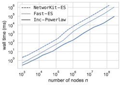
Figure 5: Average running-time of sequential Inc-Powerlaw and Edge-Switching.

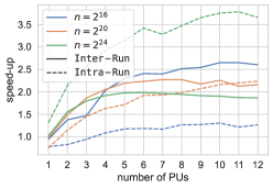
Figure 6: Speed-up of the parallel variants Inter-Run and Intra-Run over sequential Inc-Powerlaw.

Speed-up of the parallel variants

Figure 6 shows the speed-up of our Inter-Run and Intra-Run parallelizations over sequential Inc-Powerlaw. We generate degree sequences with $n=2^{k}$ for $k\in\{16,20,24\}$, measure the average running-time of the parallel variants when using $1\leq p\leq 12$ PUs (processor cores), and report the speed-up in the average running-time of the parallel variants over sequential Inc-Powerlaw.

For $p=5$ and $n=2^{24}$, we observe an Inter-Run parallelization speed-up of $2.0$; more PUs yield diminishing returns as the speed-up is limited by the number of runs until a graph is accepted which is $3.0$ on average for the aforementioned parameters. Another limiting factor is the fact that rejected runs stop prematurely. Hence, the accepting run (i) requires on average more work and (ii) forms the critical path that cannot be accelerated by Inter-Run.

For the same $n$, Intra-Run achieves a speed-up of $3.8$ for $p=11$ PUs; here, the remaining unparallelized sections limit the scalability as governed by Amdahl’s law [36]. Overall, Inter-Run yields a better speed-up if the the number of restarts is high (smaller $n$), whereas Intra-Run yields a better speed-up for larger $n$ if the overall running-time is dominated by generating the initial graph (see Table 1).

Table 1: The average number of runs until acceptance and peak speed-ups as observed in Figure 6.

$n$	runs	Inter-Run	Intra-Run
$2^{16}$	$3.9$	$2.7$ for $p=10$	$1.3$ for $p=10$
$2^{20}$	$3.3$	$2.3$ for $p=7$	$2.2$ for $p=12$
$2^{24}$	$3.0$	$2.0$ for $p=5$	$3.8$ for $p=11$

Different values of the power-law exponent $\gamma$

Next, we investigate the influence of the power-law exponent $\gamma$. The guarantees on Inc-Powerlaw’s running-time only hold for sequences with $\gamma\gtrapprox 2.88102$, so we expect a superlinear running-time for $\gamma\leq 2.88$. For $\gamma\geq 3$, the expected number of non-simple edges in the initial graph is much lower, so we expect the running-time to remain linear but with decreased constants. Figure 8 shows the average running-time of Inc-Powerlaw for sequences for various $\gamma$.

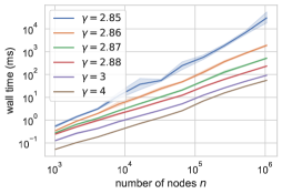
Figure 7: The average running-time of Inc-Powerlaw in dependence of $n$ for different values of $\gamma$.

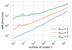
Figure 8: The average running-time of Inc-Powerlaw for sequences with minimum degree $d_{min}\in\{1,2,3\}$.

Table 2: Average number of runs until acceptance and average number of switching steps in an accepting run.

	$d_{min}=1$		$d_{min}=2$		$d_{min}=3$
$n$	runs	steps	runs	steps	runs	steps
$2^{16}$	$3.9$	$4.9$	$53.0$	$24.1$	$1160.7$	$51.0$
$2^{20}$	$3.3$	$10.2$	$18.1$	$49.6$	$164.0$	$110.8$
$2^{24}$	$3.0$	$19.0$	$9.6$	$92.8$	$43.3$	$208.5$
$2^{28}$	$2.5$	$32.3$	$5.6$	$161.6$	$16.7$	$375.3$

For $\gamma\leq 2.88$, we observe an increase in the running-time. The slope of the curve for $\gamma=2.85$ also suggests that the running-time becomes non-linear for lower values of $\gamma$. Overall, the requirement of $\gamma\gtrapprox 2.88102$ appears to be relatively strict. In particular, we observe that the higher maximum degrees of sequences with $\gamma\leq 2.85$ greatly increase the rejection probability in Phases 1 and 2.

For $\gamma\geq 3$, the average running-time decreases somewhat but remains linear. For these values of $\gamma$, we observe that the initial number of non-simple edges in the graph is small, and that the algorithm almost always accepts a graph on its first run, so the overall running-time approaches the time required to sample the initial graph with the configuration model.

Higher average degrees

The previously considered sequences drawn from an unscaled power-law distribution tend to have a rather small average degree of approximately $1.44$. On the other hand, many observed networks feature higher average degrees [4, 37]. To study Inc-Powerlaw on such networks, we sample degree sequences with minimum degree $d_{min}\in\{1,2,3\}$. For $d_{min}=2$ and $d_{min}=3$, the average degree $\overline{d}$ of the sequences increases to $\overline{d}=3.39$ and $\overline{d}=5.44$ respectively. We then let the implementation generate graphs for each choice of $d_{min}\in\{1,2,3\}$, and report the average time as a function of $n$ in Figure 8.

As a higher average degree increases the expected number of non-simple edges in the initial graph, we observe a significant increase in running-time. For instance, for $n=2^{20}$ we find that the average number of double-edges in the initial graph are $6.5$, $41.6$ and $98.8$ for $d_{min}=1,2$ and $3$, respectively, and the overall number of switching steps until a simple graph is obtained increases from $10.2$ for $d_{min}=1$ to $49.6$ for $d_{min}=2$ and to $110.8$ for $d_{min}=3$. This in turn greatly increases the chance for a rejection to occur and the number of runs until a graph is accepted (see Table 2).

However, for large values of $n\geq 2^{24}$ the effect of the higher average degrees on the running-time becomes less pronounced. This is because the probability of a rejection at any step in the algorithm decreases quite fast with $n$, thus even if the number of switching steps increases, the number of runs decreases. We can conclude that Inc-Powerlaw is efficient when generating graphs that are either very sparse ($\overline{d}\lessapprox 5$) or very large ($n\gtrapprox 2^{24}$), but the algorithm is much less efficient when generating small to medium sized graphs ($n\lessapprox 2^{24}$) with medium average degree ($\overline{d}\gtrapprox 5$).

Speed-up of Inter-Run for higher average degrees

While Inc-Powerlaw’s sequential work increases with a higher average degree, so do the number of independent runs that can be parallelized by Inter-Run. Figure 9 shows the speedup of Inter-Run over sequential Inc-Powerlaw for sequences with $d_{min}=2$ when using $2\leq p\leq 24$ PUs and $d_{min}=3$ using $2\leq p\leq 32$ PUs. For $n=2^{20}$ nodes, Inter-Run yields a speed-up of $6.4$ with $p=14$ PUs for $d_{min}=2$ and $12.8$ for $p=31$ PUs for $d_{min}=3$ (see Table 3).

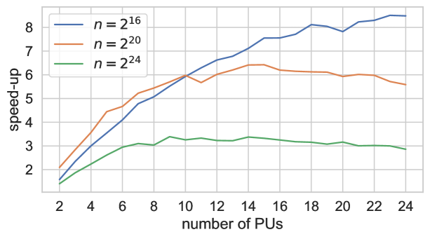
(a) Speed-ups for $d_{min}=2$.

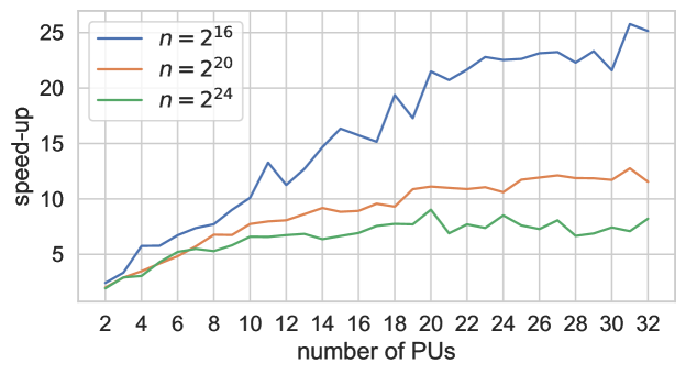
(b) Speed-ups for $d_{min}=3$.

Figure 9: Speed-up of Inter-Run for $d_{min}\in\{2,3\}$.

Table 3: Average number of runs until acceptance and peak speed-ups as observed in Figure 9.

	$d_{min}=2$		$d_{min}=3$
$n$	runs	speedup	runs	speedup
$2^{16}$	$53.0$	$8.5$ for $p=24$	$1160.7$	$25.8$ for $p=31$
$2^{20}$	$18.1$	$6.4$ for $p=14$	$164.0$	$12.8$ for $p=31$
$2^{24}$	$9.6$	$3.4$ for $p=8$	$43.3$	$9.0$ for $p=20$

As expected, we can achieve a higher speed-up for higher $d_{min}$, so we can partially mitigate the increase in running-time by taking advantage of the higher parallelizability. On the other hand, we still experience the limited scaling due to accepting runs being slower than rejecting runs.

6 Conclusions

For the first time, we provide a complete description of Inc-Powerlaw which builds on and extends previously known results [2, 16]. To the best of our knowledge, Inc-Powerlaw is the first practical implementation to sample provably uniform graphs from prescribed power-law-bounded degree sequences with $\gamma\geq 2.88102$. In an empirical study, we find that Inc-Powerlaw is very efficient for small average degrees; for larger average degrees, we observe significantly increased constants in Inc-Powerlaw’s running-time which are partially mitigated by an improved parallelizability.

While the expected running-time of Inc-Powerlaw is asymptotically optimal, we expect practical improvements for higher average degrees by improving the acceptance probability in Phases 3, 4 and 5 of the algorithm (e.g. by finding tighter lower bounds or by adding new switchings). It is also possible that the requirement on $\gamma$ could be lowered; our experiments indicate that the acceptance probability in Phases 1 and 2 should be improved to this end. Our measurements also suggest that more fine-grained parallelism may be necessary to accelerate accepting runs.

Appendix A Summary of symbols used

Symbol	Section	Remark
$[x]_{k}$	1.3	$k$-th factorial moment $[x]_{k}=\prod_{i=0}^{k-1}(x-i)$
$ij$, $\{i,j\}$	1.3	edge connecting nodes $i$ and $j$
$(i,j)$	1.3	pair connecting nodes $i$ and $j$
$m_{i,j}$	1.3	multiplicity of edge $ij$, number of pairs $(i,j)$
$v_{1}v_{2}v_{3}$	2.5	two-star centered at $v_{1}$
$v_{1}v_{2}v_{3}v_{4}$	2.6	three-star centered at $v_{1}$
$\mathbf{d}$, $d_{i}$	1.3	degree sequence $\mathbf{d}=(d_{1},\dots,d_{n})\in\mathbb{N}^{n}$
$\mathcal{G}(\mathbf{d})$	1.3	set of simple graphs matching degree sequence $\mathbf{d}$
plib	1.3	power-law distribution-bounded
$\gamma$	1.3	power-law exponent
$h$	1.3	number of heavy nodes $h=n^{1-\delta(\gamma-1)}$ where $\frac{1}{2\gamma-3}<\delta<\frac{2-3/(\gamma-1)}{4-\gamma}$
$M_{k}$	1.3	$M_{k}=\sum_{i=1}^{n}[d_{i}]_{k}$, $k$-th moment of the degree distribution
$H_{k}$	1.3	$H_{k}=\sum_{i=1}^{h}[d_{i}]_{k}$
$L_{k}$	1.3	$L_{k}=M_{k}-H_{k}$
$W_{i}$	2.1	sum of the multiplicities of heavy multi-edges incident to $i$
$W_{i,j}$	2.1	$W_{i,j}=W_{i}+2m_{i,i}-m_{i,j}$
$f(G)$	2.2	number of valid switchings on $G$
$\overline{f}(G)$	2.2	upper bound on $f(G)$
$\underline{f}(G)$	2.2	lower bound on $f(G)$
$b(G^{\prime})$	2.2	number of valid switchings that produce $G^{\prime}$
$\overline{b}(G^{\prime})$	2.2	upper bound on $b(G^{\prime})$
$\underline{b}(G^{\prime})$	2.2	lower bound on $b(G^{\prime})$
$m_{l}(G)$	2.4	number of light single loops in $G$
$m_{t}(G)$	2.4	number of light triple-edges in $G$
$m_{d}(G)$	2.4	number of light double-edges in $G$
$b(G^{\prime},\overline{V}_{i})$	2.5	number of structures in $G^{\prime}$ matching a valid switching that creates $\overline{V}_{i}$
$\underline{b}(G^{\prime};i)$	2.5	lower bound on $b(G^{\prime},\overline{V}_{i})$
$A_{2}$	2.5	let $A_{2}=\sum\nolimits_{i=1}^{d_{1}}d_{i}$, then for any node $v$, $A_{2}$ is an upper bound on the number of simple two-stars where $v$ is one of the outer nodes
$\tau$	2.6	switching type chosen in iterations of Phase 4 and 5
$\rho_{\tau}$	2.6	probability of chosing type $\tau$
$\varepsilon$	2.6	$\varepsilon=28M_{2}^{2}/M_{1}^{3}$, upper bound on the probability of choosing a type $t_{a},t_{b}$, or $t_{c}$ switching in Phase 4
$k$	2.6	number of additional pairs created by Phase 4 or 5 booster switchings
$B_{k}$	2.6	let $B_{k}=\sum_{i=1}^{d_{1}}[d_{h+i}]_{k}$, then for any node $v$, $B_{k}$ is an upper bound on the number of simple light $k$-stars where $v$ is one of the outer nodes
$\xi$	2.7	$\xi=32M_{2}^{2}/M_{1}^{3}+36M_{4}L_{4}/M_{2}L_{2}M_{1}^{2}+32M_{3}^{2}/M_{1}^{4}$, upper bound on the probability of choosing a switching type other than type $d$ or $(1,0,0)$ in Phase 5

Appendix B Additional Proofs

B.1 Correctness proofs of lower bounds

For Phases 3, 4 and 5, we use new lower bounds on the number of structures in the graph created by a valid switching.

For Phase 3, we factorize the lower bound on the number of inverse $l$-switchings used in Pld to obtain two new lower bounds $\underline{b}_{l}(G^{\prime};0)$ and $\underline{b}_{l}(G^{\prime};1)$.

Lemma B.1.

Let $\mathcal{S}$ be the class of graphs with $m_{t}$ light triple-edges, $m_{d}$ light double-edges and $m_{l}$ light single loops (and no other non-simple edges). For all $G\in\mathcal{S}$, and all light simple two-stars $v_{1}v_{2}v_{3}$ in $G$ that are created by a valid $l$-switching, we have

$$\underline{b}_{l}(\mathcal{S};0) \leq b_{l}(G,\emptyset)$$ (26)

$$\underline{b}_{l}(\mathcal{S};1) \leq b_{l}(G,v_{1}v_{2}v_{3}).$$ (27)

Proof B.2.

We have $\underline{b}_{l}(\mathcal{S};0)=L_{2}-12m_{t}d_{h}-8m_{d}d_{h}-m_{l}d_{h}^{2}$, and $b_{l}(G,\emptyset)$ is equal to the number of light simple ordered two-stars in $G$. We now show that $\underline{b}_{l}(\mathcal{S};0)$ is a lower bound on $b_{l}(G,\emptyset)$. First, each graph $G$ matching the sequence contains exactly $L_{2}$ light ordered two-stars. We then overestimate the number of two-stars that are not simple, and subtract this from $L_{2}$: a two-star $v_{1}v_{2}v_{3}$ is not simple if one of the edges $v_{1}v_{2}$ or $v_{1}v_{3}$ is a triple-edge, a double-edge or a loop. There are at most $12m_{t}d_{h}$ that contain a triple-edge, as there are $m_{t}$ ordered triple-edges ($6m_{t}$ ordered pairs), at most $d_{h}$ choices for the remaining node of the two-star (any light node has degree smaller than $d_{h}$), and $2$ ways to combine the selected pairs into the two-star as shown in Figure 2. Similarly, there are at most $8m_{d}d_{h}$ two-stars that contain a double-edge, as there are $m_{d}$ double-edges ($4m_{d}$ ordered pairs), at most $d_{h}$ choices for the remaining node and $2$ ways to combine the selected pairs into the two-star, and there are at most $m_{l}d_{h}^{2}$ two-stars that contain a loop, as there are $m_{l}$ loops and at most $d_{h}^{2}$ choices for the outer nodes of the two-star.

For the second bound, we have $\underline{b}_{l}(\mathcal{S};1)=M_{1}-6m_{t}-4m_{d}-2m_{l}-2A_{2}-4d_{1}-2d_{h}$ and $b_{l}(G,v_{1}v_{2}v_{3})$ is set to the number of simple ordered pairs $(v_{4},v_{5})$ that (a) do share nodes with the two-star $v_{1}v_{2}v_{3}$ and (b) where $v_{2}v_{4}$ and $v_{3}v_{5}$ are non-edges. Each graph $G$ matching the sequence contains exactly $M_{1}$ ordered pairs. There are at most $6m_{t}$ ordered pairs that contain a triple-edge, at most $4m_{d}$ ordered pairs that contain a double-edge and at most $2m_{l}$ ordered pairs that contain a loop. For case (a), there are at most $4d_{1}$ ordered pairs where $v_{4}\in\{v_{2},v_{3}\}$ or $v_{5}\in\{v_{2},v_{3}\}$, and at most $2d_{h}$ ordered pairs where $v_{4}=v_{1}$ or $v_{5}=v_{1}$. For case (b), we know that $A_{2}=\sum_{i=1}^{d_{1}}d_{i}$ is an upper bound on the number of two-paths $v_{2}v_{4}v_{5}$ or $v_{3}v_{5}v_{4}$ [16], so there are at most $2A_{2}$ such pairs.

For Phase 4, we use three new lower bounds $\underline{b}_{t}(G;0)$, $\underline{b}_{t}(G;1)$ and $\underline{b}_{\tau}(G;i+1)$.

Lemma B.3.

Let $\mathcal{S}$ be the class of graphs with $m_{t}$ light triple-edges and $m_{d}$ light double-edges (and no other non-simple edges). For all $G\in\mathcal{S}$, all simple three-stars $v_{1}v_{3}v_{5}v_{7}$ in $G$, and all triplets with $1\leq i\leq k$ additional pairs $\overline{V}_{i+1}(S)=(v_{1}v_{3}v_{5}v_{7}v_{2}v_{4}v_{6}v_{8},\dots,v_{6+2i-1}v_{6+2i})$ in $G$ that are created by a valid Phase 4 switching $S$, we have

$$\underline{b}_{t}(\mathcal{S};0) \leq b_{t}(G,\emptyset)$$ (28)

$$\underline{b}_{t}(\mathcal{S};1) \leq b_{t}(G,v_{1}v_{3}v_{5}v_{7})$$ (29)

$$\underline{b}_{\tau}(\mathcal{S};i+1) \leq b_{\tau}(G,\overline{V}_{i+1}(S)).$$ (30)

Proof B.4.

We have $\underline{b}_{t}(\mathcal{S};0)=M_{3}-18m_{t}d_{1}^{2}-12m_{d}d_{1}^{2}$ and $b_{t}(G,\emptyset)$ is set to the number of simple ordered three-stars in $G$. Analogously to Lemma 1, we show that $\underline{b}_{t}(\mathcal{S};0)$ is a lower bound on $b_{t}(G,\emptyset)$ by starting with $M_{3}$, the number of ordered three-stars in a graph $G$ matching the sequence and then subtracting an overestimate of the number of non-simple three-stars. The only non-simple three-stars contain a triple-edge or a double-edge. There are at most $18m_{t}d_{1}^{2}$ non-simple three-stars that contain a triple-edge, as there are $m_{t}$ triple-edges in $G$, at most $d_{1}$ choices for each of the two remaining outer nodes, and $18$ ways to label the star as shown in 3(a). Similarly, there are at most $12m_{d}d_{1}^{2}$ three-stars that contain a double-edge.

For the second bound, we have $\underline{b}_{t}(G^{\prime};1)=L_{3}-18m_{t}d_{h}^{2}-12m_{d}d_{h}^{2}-B_{3}-3(m_{t}+m_{d})B_{2}-d_{h}^{3}-9B_{2}$, and $b_{t}(G,v_{1}v_{3}v_{5}v_{7})$ is equal to the number of light simple ordered three-stars that a) do not share any nodes with the three-star $v_{1}v_{3}v_{5}v_{7}$ created by $S$, b) have no edge $v_{1}v_{2}$ and no multi-edges $v_{3}v_{4}$, $v_{5}v_{6}$, $v_{7}v_{8}$. Each graph matching the sequence contains exactly $L_{3}$ light ordered simple three-stars. Analogous to $\underline{b}_{t}(\mathcal{S};0)$, there are at most $18m_{t}d_{h}^{2}+12m_{d}d_{h}^{2}$ light three-stars that are not simple. There are at most $d_{h}^{3}+9B_{2}$ light simple ordered three-stars $v_{2}v_{4}v_{6}v_{8}$ of case a): first, if $v_{2}=v_{1}$, then there are at most $d_{h}^{3}$ choices for the outer nodes. In addition, we know that for each node $v_{4}$ in $G$, there are at most $B_{2}=\sum_{i=1}^{d_{1}}[d_{h+i}]_{2}$ light simple two-stars $v_{2}v_{6}v_{8}$ where $v_{2}v_{4}$ is an edge [16], so there are at most $9B_{2}$ three-stars where $v_{4},v_{6},v_{8}\in\{v_{3},v_{5},v_{7}\}$. The only remaining case is if $v_{2}\in\{v_{3},v_{5},v_{7}\}$, or if any of $v_{4},v_{6},v_{8}=v_{1}$, but in this case $v_{1}v_{2}$ is an edge, so this falls under case b). For case b), it suffices to subtract $B_{3}+3(m_{t}+m_{d})B_{2}$ three-stars: we know that for each node $v_{1}$ in $G$, there are at most $B_{3}=\sum_{i=1}^{d_{1}}[d_{h+i}]_{3}$ light simple three-stars $v_{2}v_{4}v_{6}v_{8}$ where $v_{2}v_{1}$ is an edge. For a three-star where any of $v_{3}v_{4}$, $v_{5}v_{6}$, $v_{7}v_{8}$ is a multi-edge, we have at most $3(m_{t}+m_{d})B_{2}$ choices, as there are $m_{t}+m_{d}$ multi-edges in $G$ and choices for the first outer node, and at most $B_{2}$ choices for the center and the two remaining outer nodes.

For the third bound, we have $\underline{b}_{\tau}(\mathcal{S};i+1)=M_{1}-6m_{t}-4m_{d}-16d_{1}-4(i-1)d_{1}-2A_{2}$, and $b_{\tau}(G,\overline{V}_{i+1}(S))$ is equal to the number of simple ordered pairs in $G$, that a) do not share any nodes with the triplet, or the previous $i-1$ pairs, and b) have no forbidden edges with the triplet. First, each graph matching the sequence contains exactly $M_{1}$ ordered pairs. At most $6m_{t}$ of those pairs are in a triple-edge, and at most $4m_{d}$ pairs are in a double-edge. For case a), there are at most $16d_{1}$ ordered pairs that share a node with the triplet, as for each of the $8$ nodes of the triplet, there are at most $d_{1}$ choices for the second node of the simple pair and $2$ ways to label the pair. Similarly, there are at most $4(i-1)$ pairs that share a node with the $i-1$ pairs relaxed in the previous steps. Finally, there are at most $2A_{2}$ pairs of case b): each of the two nodes in the pair cannot have an edge with one designated node of the triplet, and starting from that node, there are at most $A_{2}$ pairs connected to it via an edge.

In Phase 5, we use three new lower bounds $\underline{b}_{d}(G;0)$, $\underline{b}_{d}(G;1)$ and $\underline{b}_{\tau}(G;k+1)$.

Lemma B.5.

Let $\mathcal{S}$ be the class of graphs with $m_{d}$ light double-edges (and no other non-simple edges). For all $G\in\mathcal{S}$, all simple two-stars $v_{1}v_{3}v_{5}$ in $G$, and all doublets with $1\leq i\leq k$ additional pairs $\overline{V}_{i+1}(S)=(v_{1}v_{3}v_{5}v_{2}v_{4}v_{6},\dots,v_{4+2i-1}v_{4+2i})$ in $G$ that are created by a valid Phase 5 switching $S$, we have

$$\underline{b}_{d}(\mathcal{S};0) \leq b_{d}(G,\emptyset)$$ (31)

$$\underline{b}_{d}(\mathcal{S};1) \leq b_{d}(G,v_{1}v_{3}v_{5})$$ (32)

$$\underline{b}_{\tau}(\mathcal{S};i+1) \leq b_{\tau}(G,\overline{V}_{i+1}(S)).$$ (33)

Proof B.6.

We have $\underline{b}_{d}(G^{\prime};0)=M_{2}-8m_{d}d_{1}$, and $b_{d}(G,\emptyset)$ is set to the number of simple ordered two-stars in $G$. We now show that $\underline{b}_{d}(G^{\prime};0)$ is a lower bound on $b_{d}(G,\emptyset)$. There are $M_{2}$ ordered two-stars in a graph $G$ matching the sequence. Of these, the only ones that are not simple are the ones that contain a double-edge, and $G$ can contain at most $8m_{d}d_{1}$ such two-stars.

For the second bound, we have $\underline{b}_{d}(G;1)=L_{2}-8m_{d}d_{h}-6B_{1}-3d_{h}^{2}$, and $b_{d}(G,v_{1}v_{3}v_{5})$ is equal to the number of light simple ordered two-stars in that do not share any nodes with the two-star $v_{1}v_{3}v_{5}$. Similar to the first step above, $G$ contains exactly $L_{2}$ light ordered two-stars, and at most $8m_{d}d_{h}$ light ordered two-stars that are not simple. The only remaining cases are two-stars $v_{2}v_{4}v_{6}$ that share any nodes with the first two-star. First, there are at most $6B_{1}$ two-stars where $v_{4},v_{6}\in\{v_{1},v_{3},v_{5}\}$, as $B_{1}$ is an upper bound on the number of pairs $v_{2}v_{4}$ or $v_{2}v_{6}$ where $v_{4}$ or $v_{6}$ are connected to one of $v_{1},v_{3},v_{5}$ via an edge. The other remaining case is $v_{2}\in\{v_{1},v_{3},v_{5}\}$. In this case, there are at most $d_{h}^{2}$ choices for the remaining nodes of the two-star, so in total there are at most $3d_{h}^{2}$ such two-stars.

The proof for $\underline{b}_{\tau}(\mathcal{S};i+1)$ is analogous to the proof for the similar bound in Phase 4 (see above).

References

- [1] M. Alam, M. Khan, A. Vullikanti, and M. Marathe. An efficient and scalable algorithmic method for generating large: scale random graphs. In SC. IEEE Computer Society, 2016. doi:10.1109/SC.2016.31.
- [2] A. Arman, P. Gao, and N. C. Wormald. Fast uniform generation of random graphs with given degree sequences. In FOCS. IEEE Computer Society, 2019. doi:10.1109/FOCS.2019.00084.
- [3] M. Axtmann, S. Witt, D. Ferizovic, and P. Sanders. Engineering in-place (shared-memory) sorting algorithms. CoRR, abs/2009.13569, 2020.
- [4] A. Barabási et al. Network science. Cambridge university press, 2016.
- [5] M. Bayati, J. H. Kim, and A. Saberi. A sequential algorithm for generating random graphs. Algorithmica, 58(4), 2010. doi:10.1007/s00453-009-9340-1.
- [6] A. Békéssy, P. Békéssy, and J. Komlós. Asymptotic enumeration of regular matrices. Stud. Sci. Math. Hungar., 7, 1972.
- [7] E. A. Bender and E. R. Canfield. The asymptotic number of labeled graphs with given degree sequences. J. Comb. Theory, Ser. A, 24(3), 1978. doi:10.1016/0097-3165(78)90059-6.
- [8] M. H. Bhuiyan, J. Chen, M. Khan, and M. V. Marathe. Fast parallel algorithms for edge-switching to achieve a target visit rate in heterogeneous graphs. In 43rd Int. Conf. on Parallel Processing, ICPP 2014. IEEE Computer Society, 2014. doi:10.1109/ICPP.2014.15.
- [9] B. Bollobás. A probabilistic proof of an asymptotic formula for the number of labelled regular graphs. Eur. J. Comb., 1(4), 1980. doi:10.1016/S0195-6698(80)80030-8.
- [10] B. Bollobás. Random graphs. Academic Press, 1985.
- [11] C. J. Carstens, M. Hamann, U. Meyer, M. Penschuck, H. Tran, and D. Wagner. Parallel and I/O-efficient randomisation of massive networks using global curveball trades. In ESA, volume 112 of LIPIcs, 2018. doi:10.4230/LIPIcs.ESA.2018.11.
- [12] F. Chung and L. Lu. Connected components in random graphs with given expected degree sequences. Annals of Combinatorics, 6(2), 2002. doi:10.1007/pl00012580.
- [13] C. Cooper, M. E. Dyer, and C. S. Greenhill. Sampling regular graphs and a peer-to-peer network. Comb. Probab. Comput., 16(4), 2007. doi:10.1017/S0963548306007978.
- [14] D. Funke, S. Lamm, U. Meyer, M. Penschuck, P. Sanders, C. Schulz, D. Strash, and M. von Looz. Communication-free massively distributed graph generation. J. Parallel Distributed Comput., 131, 2019. doi:10.1016/j.jpdc.2019.03.011.
- [15] P. Gao and N. C. Wormald. Uniform generation of random regular graphs. In FOCS. IEEE Computer Society, 2015. doi:10.1109/FOCS.2015.78.
- [16] P. Gao and N. C. Wormald. Uniform generation of random graphs with power-law degree sequences. In SODA. SIAM, 2018. doi:10.1137/1.9781611975031.114.
- [17] C. Gkantsidis, M. Mihail, and E. W. Zegura. The Markov chain simulation method for generating connected power law random graphs. In ALENEX. SIAM, 2003.
- [18] N. J. Gotelli and G. R. Graves. Null models in ecology. Smithsonian Institution, 1996.
- [19] C. S. Greenhill. The switch Markov chain for sampling irregular graphs (extended abstract). In SODA. SIAM, 2015. doi:10.1137/1.9781611973730.103.
- [20] M. Hamann, U. Meyer, M. Penschuck, H. Tran, and D. Wagner. I/o-efficient generation of massive graphs following the LFR benchmark. ACM J. Exp. Algorithmics, 23, 2018. doi:10.1145/3230743.
- [21] S. Janson. The probability that a random multigraph is simple. Combinatorics, Probability and Computing, 18(1-2), 2009.
- [22] M. Jerrum and A. Sinclair. Fast uniform generation of regular graphs. Theor. Comput. Sci., 73(1), 1990. doi:10.1016/0304-3975(90)90164-D.
- [23] R. Kannan, P. Tetali, and S. S. Vempala. Simple Markov-chain algorithms for generating bipartite graphs and tournaments. Random Struct. Algorithms, 14(4), 1999.
- [24] J. H. Kim and V. H. Vu. Generating random regular graphs. Comb., 26(6), 2006. doi:10.1007/s00493-006-0037-7.
- [25] A. Lancichinetti and S. Fortunato. Benchmarks for testing community detection algorithms on directed and weighted graphs with overlapping communities. Phys. Rev. E, 80(1), 2009. doi:10.1103/physreve.80.016118.
- [26] D. Lemire. Fast random integer generation in an interval. ACM Trans. Model. Comput. Simul., 29(1), 2019. doi:10.1145/3230636.
- [27] P. Mahadevan, D. V. Krioukov, K. R. Fall, and V. Vahdat. Systematic topology analysis and generation using degree correlations. In SIGCOMM. ACM, 2006.
- [28] B. D. McKay and N. C. Wormald. Uniform generation of random regular graphs of moderate degree. J. Algorithms, 11(1), 1990. doi:10.1016/0196-6774(90)90029-E.
- [29] J. C. Miller and A. A. Hagberg. Efficient generation of networks with given expected degrees. In WAW, volume 6732 of Lecture Notes in Computer Science, 2011. doi:10.1007/978-3-642-21286-4_10.
- [30] R. Milo. Network motifs: Simple building blocks of complex networks. Science, 298(5594), 2002. doi:10.1126/science.298.5594.824.
- [31] R. Milo, N. Kashtan, S. Itzkovitz, M. E. J. Newman, and U. Alon. On the uniform generation of random graphs with prescribed degree sequences. December 2003. arXiv:cond-mat/0312028.
- [32] S. Moreno, J. J. Pfeiffer III, and J. Neville. Scalable and exact sampling method for probabilistic generative graph models. Data Mining and Knowledge Discovery, 32(6), 2018. doi:10.1007/s10618-018-0566-x.
- [33] M. E. J. Newman. Networks: An Introduction. Oxford University Press, 2010. doi:10.1093/ACPROF:OSO/9780199206650.001.0001.
- [34] M. Penschuck, U. Brandes, M. Hamann, S. Lamm, U. Meyer, I. Safro, P. Sanders, and C. Schulz. Recent advances in scalable network generation. CoRR, abs/2003.00736, 2020.
- [35] J. Ray, A. Pinar, and C. Seshadhri. Are we there yet? when to stop a markov chain while generating random graphs. In WAW, volume 7323 of Lecture Notes in Computer Science, 2012. doi:10.1007/978-3-642-30541-2_12.
- [36] D. P. Rodgers. Improvements in multiprocessor system design. In ISCA. IEEE Computer Society, 1985.
- [37] R. A. Rossi and N. K. Ahmed. The network data repository with interactive graph analytics and visualization. In AAAI. AAAI Press, 2015.
- [38] P. Sanders. Random permutations on distributed, external and hierarchical memory. Inf. Process. Lett., 67(6), 1998.
- [39] W. E. Schlauch, E. Á. Horvát, and K. A. Zweig. Different flavors of randomness: comparing random graph models with fixed degree sequences. Social Network Analysis and Mining, 5(1), 2015. doi:10.1007/s13278-015-0267-z.
- [40] J. Singler and B. Konsik. The GNU libstdc++ parallel mode: software engineering considerations. In Int. workshop on Multicore software eng., 2008.
- [41] I. Stanton and A. Pinar. Sampling graphs with a prescribed joint degree distribution using Markov chains. In ALENEX. SIAM, 2011.
- [42] C. L. Staudt, A. Sazonovs, and H. Meyerhenke. Networkit: A tool suite for large-scale complex network analysis. Netw. Sci., 4(4), 2016. doi:10.1017/nws.2016.20.
- [43] A. Steger and N. C. Wormald. Generating random regular graphs quickly. Comb. Probab. Comput., 8(4), 1999.
- [44] G. Strona, D. Nappo, F. Boccacci, S. Fattorini, and J. San-Miguel-Ayanz. A fast and unbiased procedure to randomize ecological binary matrices with fixed row and column totals. Nature communications, 5(1), 2014.
- [45] G. Tinhofer. On the generation of random graphs with given properties and known distribution. Appl. Comput. Sci., Ber. Prakt. Inf, 13:265–297, 1979.
- [46] N. D. Verhelst. An efficient MCMC algorithm to sample binary matrices with fixed marginals. Psychometrika, 73(4), 2008.
- [47] F. Viger and M. Latapy. Efficient and simple generation of random simple connected graphs with prescribed degree sequence. J. Complex Networks, 4(1), 2016. doi:10.1093/comnet/cnv013.
- [48] J. Y. Zhao. Expand and contract: Sampling graphs with given degrees and other combinatorial families. 2013. arXiv:1308.6627.