Classical conformal blocks, Coulomb gas integrals and Richardson–Gaudin models

Abstract

Virasoro conformal blocks are universal ingredients of correlation functions of two-dimensional conformal field theories (2d CFTs) with Virasoro symmetry. It is acknowledged that in the (classical) limit of large central charge of the Virasoro algebra and large external, and intermediate conformal weights with fixed ratios of these parameters Virasoro blocks exponentiate to functions known as Zamolodchikovs’ classical blocks. The latter are special functions which have awesome mathematical and physical applications. Uniformization, monodromy problems, black holes physics, quantum gravity, entanglement, quantum chaos, holography, ${\cal N}=2$ gauge theory and quantum integrable systems (QIS) are just some of contexts, where classical Virasoro blocks are in use. In this paper, exploiting known connections between power series and integral representations of (quantum) Virasoro blocks, we propose new finite closed formulae for certain multi-point classical Virasoro blocks on the sphere. Indeed, combining classical limit of Virasoro blocks expansions with a saddle point asymptotics of Dotsenko–Fateev (DF) integrals one can relate classical Virasoro blocks with a critical value of the “Dotsenko–Fateev matrix model action”. The latter is the “DF action” evaluated on a solution of saddle point equations which take the form of Bethe equations for certain QIS (Gaudin spin models). A link with integrable models is our main motivation for this research line. For instance, analogous quantities as the “DF on-shell action” appear in 2d CFT realization of the so-called Richardson’s solution of the reduced BCS model describing physics of ultra-small superconducting grains. Precisely, the Richardson solution and its particular limit characterizing the rational Gaudin model have known implementation in 2d CFT in terms of a free field representation of certain (perturbed and unperturbed) WZW blocks. The WZW analogue of the “DF on-shell action” appears here and plays a crucial role, it is a generating function for eigenvalues of quantum integrals of motion. An exploration of relationships between power expansions and Coulomb gas representations of the aforementioned WZW blocks could pave a way for new analytical tools useful in the study of models of the Richardson–Gaudin type.

1 Introduction

Conformal field theory in two dimensions (2d CFT or CFT₂) yields an effective description of critical phenomena in two-dimensional statistical systems DiFMS and describes worldsheet dynamics of relativistic strings Pol . Two-dimensional CFT has also found use in the condensed matter physics, in particular as a tool to study states of the fractional quantum Hall effect (FQHE). For instance, the Laughlin wave functions Laughlin can be represented by certain conformal blocks calculated within a free field realization. Conformal blocks (see below) are model independent 2d CFT “special functions” defined entirely within a representation theoretic framework.

During the last decade CFT₂ has been used in completely new contexts. Before mentioning them, let us recall that in 2d CFT, like in any quantum field theory, basic objects being studied are correlation functions. In 2d CFT correlation functions are defined on the Riemann surfaces $C_{g,n}$ with genus $g$ and $n$ punctures. Due to conformal symmetry correlators of any 2d CFT model can be written as a sum (or an integral for theories with a continuous spectrum) which includes terms consisting of conformal blocks times the so-called structure constants. The conformal blocks ${\cal F}\!\left({\boldsymbol{\Delta}},\underline{\boldsymbol{\Delta}},c\,|\,\cdot\,\right)$ on $C_{g,n}$ depend on the central charge $c$ of the Virasoro algebra, the so-called external conformal weights $\boldsymbol{\Delta}:=\left\{\Delta_{i}\right\}_{i=1}^{n}$ the weights $\underline{\boldsymbol{\Delta}}:=\left\{{\underline{\Delta}}_{p}\right\}_{p=1}^{3g-3+n}$ in the intermediate channels, the vertex operators locations and modular parameters in case of surfaces with $g>0$. Conformal blocks are fully determined by the underlying conformal symmetry. These functions have an interesting analytic structure, although it is not completely understood yet. In general, they can be expressed only as a formal power series and no closed formula is known for its coefficients. A list of analytic properties of conformal blocks which still require a deeper understanding contains the following problems: convergence issues of series defining conformal blocks, recurrence relations for coefficients, operator realization, integral representations, analytic continuations, classical limit.

From the point of view of applications the problem of calculation of the classical limit of the conformal blocks is currently the central issue concerning these functions. In the classical limit the central charge tends to infinity,

$$c\;\longrightarrow\;\infty$$ (1)

and it is assumed, that

• the weights are “heavy”, i.e., $\frac{\Delta_{i}}{c}={\rm const.}\;$, $\frac{{\underline{\Delta}}_{p}}{c}={\rm const.}\;$ $\forall\;i,p$ or

• the external weights are heavy (as above) and “light”, i.e., $c^{-1}\Delta_{k}^{\rm light}\to 0\;$ for some $k\in\{1,\ldots,n\}$ or

• the weights are fixed, i.e., $\Delta_{i}={\rm const.}\;$, ${\underline{\Delta}}_{p}={\rm const.}\;$ $\forall\;i,p$.

For the standard parameterization of the central charge:

$$c\;=\;1+6Q^{2},\;\;\;\;\;\;\;\;\;\;Q\;=\;b+\frac{1}{b}$$ (2)

the limit (1) corresponds to $b\to 0$ or $b\to\infty$. In this parameterization the heavy weights are defined as follows:

$$(\Delta_{i},{\underline{\Delta}}_{p})=\frac{1}{b^{2}}(\delta_{i},{\underline{\delta}}_{p}),\; \;\delta_{i},{\underline{\delta}}_{p}={\cal O}(b^{0})\;\;\;{\rm if}\;\;\;b\to 0,$$ (3)

$$(\Delta_{i},{\underline{\Delta}}_{p})=b^{2}(\delta_{i},{\underline{\delta}}_{p}),\; \;\delta_{i},{\underline{\delta}}_{p}={\cal O}(b^{0})\;\;\;{\rm if}\;\;\;b\to\infty.$$ (4)

In the first case the light conformal weights $\Delta_{k}^{\rm light}$ obey $\lim_{b\to 0}b^{2}\Delta^{\rm light}_{k}=0$, while in the second case we have, $\lim_{b\to\infty}b^{-2}\Delta^{\rm light}_{k}=0$. In the classical limit conformal blocks behave as follows.

• If all the weights are heavy, then in the classical limit the blocks exponentiate to functions known as Zamolodchikovs’ ZZ5 classical conformal blocks:

  $$\boxed{{\cal F}\!\left(\{\Delta_{i}\},\{{\underline{\Delta}_{p}}\},c\,|\,\cdot\,\right)\;\stackrel{{\scriptstyle b\to\infty}}{{\sim}}\;{\rm e}^{b^{2}f\left(\{\delta_{i}\},\{{\underline{\delta}_{p}}\}|\,\cdot\,\right)}}$$ (5)

  (or analogously for $b\to 0$, where $b^{2}$ is replaced by $b^{-2}$ and relations (3) are assumed).

• If the external weights are heavy and light, $\{\Delta_{i}\}=\{\Delta_{l}\}\cup\{\Delta_{k}^{\rm light}\}$, then in the classical limit the blocks decompose into a product of the “light contribution” $\Psi_{\rm light}\left(\cdot\right)$ and the exponent of the classical block:

  $$\boxed{{\cal F}\!\left(\{\Delta_{l}\}\cup\{\Delta_{k}^{\rm light}\},\{{\underline{\Delta}_{p}}\},c\,|\,\cdot\,\right)\;\stackrel{{\scriptstyle b\to\infty}}{{\sim}}\Psi_{\rm light}\left(\cdot\right)\,{\rm e}^{b^{2}f\left(\{\delta_{l}\},\{{\underline{\delta}_{p}}\}|\,\cdot\,\right)}}$$ (6)

  (or analogously for $b\to 0$, where $b^{2}$ is replaced by $b^{-2}$ and relations (3) are assumed).

• If all the weights are fixed, then in the large central charge limit (1) conformal blocks reduce to the so-called global blocks, i.e., contributions to the correlation functions from representations of the $\mathfrak{sl}(2,\mathbb{C})$ algebra which is a global subalgebra of the Virasoro algebra.

When commenting on the above statements, it should first be stressed that the calculation of the global limit of conformal blocks (point (C) above) is incomparably simpler than a proof of (5) and (6). For example, a four-point block on the sphere reduces in this limit to a hypergeometric function. Second, although asymptotics (5) and (6) are confirmed by the classical limit of the quantum Liouville field theory (in the sense of saddle points of the correlation functions) and resulting from (5), (6) consequences, formulae (5) and (6) should be treated as conjectures rather than rigorous mathematical theorems. Third, it is worth noting that new results have recently been obtained in this field. For example, using the oscillator representation, it was possible to demonstrate an exponentiation of the spherical four-point block in the classical limit BDK . A mechanism of the factorization (6) has been studied deeper in the case of the five-point spherical block containing four heavy external weights and one light external degenerate weight PPNPB . Finally, conjectures (5) and (6) have recently been extended to the so-called irregular conformal blocks LN ; PP1 ; PP2 ; PP3 .

For a long time classical conformal blocks were known only to specialists dealing with the Liouville theory and its applications in the uniformization theory of Riemann surfaces (see e.g. ZZ5 ; HJP ; HJ ). In the last few years the classical limit of conformal blocks has appeared in novel mathematical contexts and has been applied as a tool in the study of many fundamental problems of contemporary theoretical physics. Some of these contexts and applications are cited below.

The novel mathematical contexts with classical blocks are for instance: the theory of the KdV equation WH ; the problem of isomonodromic deformations of the Fuchs equations Teschner:2017rve , and newly discovered properties of the Painlevé VI equation Litvinov:2013sxa related to that problem. Also monodromy problems for the Fuchs equations, implicitly unrelated to uniformization, which have classical blocks as a solution, have been investigated at intensive rate (see e.g. Menotti:2014kra ; Menotti:2016jut ; Menotti:2018jsy ; HK ).

In classical and quantum physics of black holes the classical limit of conformal blocks is applied in the study of scattering problems of classical fields in geometries of certain black holes (see e.g. daCunha:2015fna ; daCunha:2015ana ; Novaes:2014lha ; Amado:2017kao ), and in the analysis of the famous information paradox within 3-dimensional quantum gravity by means of the methods of the dual theory, namely CFT₂ (see e.g. Anous:2016kss ; CHKL ).

The classical blocks have holographic counterparts via AdS₃/CFT₂ correspondence (see e.g. Alkalaev:2016rjl ; Alkalaev:2016ptm ; Alkalaev:2015fbw ; Alkalaev:2015lca ; Alkalaev:2015wia ; AlkPav ). Moreover, the classical limit and the classical blocks appear here: in holographic calculations of entanglement entropy on the 2d CFT side (see the crucial paper Hartman:2013mia and e.g. Asplund:2014coa ; Banerjee:2016qca ; MH ); in a holographic interpretation of conformal bootstrap Ver ; in the study of holographic 2d CFTs (see e.g. HartmanIII ; Chang:2015qfa ; Chang:2016ftb ); in tests of eigenstate thermalization hypothesis (ETH) FW ; FKW ; FKap ; LDL .

Regardless of the holographic context, the classical limit of conformal blocks appears in the study of universal properties of the entanglement entropy in 2d CFT (cf. Hartman:2013mia and e.g. TakaK ; Kusuki ; Kusuki2 ). The entanglement entropy is a measure of how quantum information is stored in a quantum state. The entanglement entropy can be defined in quantum mechanics and in the quantum field theory including quantum gravity.

Black holes physics, three-dimensional quantum gravity, entanglement and holography are not all the current hot topics of theoretical physics in which the classical limit of conformal blocks is applied. These techniques also appear in the research on quantum chaos (see the seminal paper  RobStan ), the so-called topological strings AKPT ; AKPT2 ; AKP and in the context of matrix models (cf. BMT ; Rim:2015tsa ; Rim:2015aha ). In addition, it turns out that classical conformal blocks have their counterparts in supersymmetric ${\cal N}=2$ Yang–Mills theories and in the theory of quantum integrable systems.

Indeed, in 2009 an amazing discovery known as the AGT correspondence AGT was made. The AGT conjecture states that the Liouville field theory correlators on the Riemann surface $C_{g,n}$ with genus $g$ and $n$ punctures can be identified with the partition functions of the class ${\cal S}_{g,n}$ of four-dimensional ${\cal N}=2$ supersymmetric SU(2) quiver gauge theories. A significant part of the AGT conjecture is an exact correspondence between the Virasoro blocks on $C_{g,n}$ and the instanton sectors of the Nekrasov partition functions N ; NekraOkun of the gauge theories ${\cal S}_{g,n}$. The AGT relations are provided when an appropriate identification is established between the parameters (see the diagram below). In particular, the conformal weights $\Delta_{\alpha}$ in the intermediate channels are expressed in terms of the vacuum expectation values ${\bf a}$ of scalar fields in vector multiplets; the external weights $\Delta_{\beta}$ are functions of masses ${\bf m}$ of the matter fields; locations of the vertex operators correspond to complexified gauge couplings; the background charge $Q$ and therefore the central charge $c=1+6Q^{2}$ are the functions of the $\Omega$ background parameters: $\epsilon_{1},\epsilon_{2}$ or equivalently the quantum parameter of the Liouville theory is $b^{2}=\epsilon_{2}/\epsilon_{1}$.

$$\begin{tabular}[]{|c|}\hline\cr${\sf Liouville}\;{\sf correlation}\;{\sf function}$\\ $\left\langle\prod\limits_{a=1}^{n}V_{\beta_{a}}\right\rangle_{C_{g,n}}^{\sf LFT}$\\ ${\sf on}\;C_{g,n}-{\sf Riemann}\;{\sf surface}$\\ ${\sf with}\;{\sf genus}\;g\;{\sf and}\;n\;{\sf punctures}$\\ \hline\cr\end{tabular}\;\;=\;\;\begin{tabular}[]{|c|}\hline\cr${\sf Partition}\;{\sf function}\;Z_{{\cal S}(g,n)}$\\ ${\sf of}\;{\sf the}\;{\sf class}\;{\cal S}(g,n)\;{\sf of}\;4d$\\ $(\Omega-{\sf deformed})\;{\cal N}=2\;{\sf SUSY}$\\ ${\sf SU}(2)\;{\sf quiver}\;{\sf gauge}\;{\sf theories}$\\ \hline\cr\end{tabular}$$

$$\begin{tabular}[]{|c|}\hline\cr${\sf Virasoro}\;{\sf conformal}\;{\sf block}$\\ ${\cal F}_{1+6Q^{2},\alpha}[\beta]({\sf Z})\;{\sf on}\;C_{g,n};$\\ $\alpha\equiv(\alpha_{1},\ldots,\alpha_{3g-3+n}),$\\ $\beta\equiv(\beta_{1},\ldots,\beta_{n}),$\\ ${\sf Z}=(z_{1},\ldots,z_{3g-3+n}),$\\ $\Delta_{\alpha}=\alpha(Q-\alpha),\;Q=b+b^{-1}$\\ \hline\cr\end{tabular}=\begin{tabular}[]{|c|}\hline\cr${\sf Nekrasov}\;{\sf instanton}\;{\sf partition}\;{\sf function}$\\ $\mathcal{Z}_{{\sf inst}}({\sf Z},{\bf a},{\bf m};\epsilon_{1},\epsilon_{2});$\\ ${\bf a}=(a_{1},\ldots,a_{3g-3+n}),$\\ ${\bf m}=(m_{1},\ldots,m_{n}),$\\ ${\sf Z}=(z_{i}=\exp 2\pi\tau_{i})_{i=1,\ldots,3g-3+n},$\\ $(\epsilon_{1}+\epsilon_{2})^{2}/(\epsilon_{1}\epsilon_{2})=Q\Longleftrightarrow\;\sqrt{\epsilon_{2}/\epsilon_{1}}=b$\\ \hline\cr\end{tabular}$$

The AGT correspondence works at the level of the quantum Liouville field theory (LFT). At this point a question can be asked about what happens if we proceed to the classical limit of the Liouville theory. It turns out that the classical limit of LFT correlators corresponds to the known limit of partition functions of supersymmetric gauge theories — the so-called Nekrasov–Shatashvili limit NS:2009 . In particular, a consequence of that correspondence is that the classical conformal blocks can be identified with the instanton sectors of the effective twisted superpotentials. The latter quantities determine the low energy effective dynamics of the two-dimensional gauge theories restricted to the $\Omega$-background. The twisted superpotentials play also a pivotal role in another duality, the Bethe/Gauge correspondence NS:2009 . As a result of that duality, the twisted superpotentials are identified with the Yang–Yang functions of the corresponding quantum integrable systems (QIS). These functions are potentials for the so-called Bethe equations which describe spectra of quantum integrable models. Hence, combining the classical/Nekrasov–Shatashvili limit of the AGT duality and the Bethe/Gauge correspondence, one gets thus the triple correspondence which links the classical blocks to the twisted superpotentials and then to the Yang–Yang (YY) functions. Precisely, we have two options here. First, let us note that the 2-particle QIS are just quantum–mechanical systems. In this case classical Virasoro blocks and twisted superpotentials are determined by eigenvalues of appropriate Schrödinger operators,

2dCFT	${\rm 2d}\;{\cal N}=2\;$SU(2) SYM	2-particle QIS
classical Virasoro blocks	twisted superpotentials	spectra of Schrödinger operators

Secondly, if we take the classical/Nekrasov–Shatashvili limit of the generalized AGT conjecture Wyllard:2009hg then the above-mentioned correspondence can be extended to the following

2dCFT	${\rm 2d}\;{\cal N}=2$ SU(N) SYM	${\rm N}$-particle QIS
classical Toda blocks	twisted superpotentials	Yang–Yang functions

where on the gauge theory side there are supersymmetric ${\cal N}=2$ ${\rm SU(N)}$ theories. Here, on the one hand, the twisted superpotentials ${\cal W}^{\rm SU(N)}$ of the ${\rm SU(N)}$ gauge theories are the Yang–Yang functions for the N-particle QIS. On the other hand, ${\cal W}^{\rm SU(N)}$ should correspond to classical Toda blocks.

So, taking into account applications, any new method of computing classical blocks and/or any new result concerning these functions can be of great use. In this paper we propose new finite expressions for certain multi-point classical Virasoro blocks on the sphere. Our proposal is based on the Mironov–Morozov–Shakirov identities MMS connecting power series representations of Virasoro blocks and their Dotsenko–Fateev integral representations. The main results of this work are conjectured relations (64) and (76) expressing classical Virasoro blocks in terms of saddle point values of Dotsenko–Fateev integrals.

A particular motivation and inspiration for the present paper is one yet more possible use of classical conformal blocks that was not mentioned above. In the first paragraph of the introduction it is mentioned that 2d CFT has applications in condensed matter physics, for example in FQHE, where the Laughlin wave functions can be represented by certain conformal blocks calculated within a free field realization. Interestingly, an idea of representing quantum states by conformal blocks works great, when it is applied to characterize eigenstates of certain many-body quantum Hamiltonians describing pairing force interactions (Cooper pairs BCS ) or systems of interacting spins (Gaudin magnets Gaudin1 ; Gaudin2 ). This concept has been used for the first time by Sierra in the seminal paper Sierra:1999mp , where he proposed a connection between 2d CFT and the exact solution, and integrability of the so-called reduced BCS model defined by the Hamiltonian:

$$\hat{\rm H}_{\rm rBCS}=\sum\limits_{j,\sigma=\pm}\varepsilon_{j\sigma}c_{j\sigma}^{\dagger}c_{j\sigma}-gd\sum\limits_{j,j^{\prime}}c_{j+}^{\dagger}c_{j-}^{\dagger}c_{j^{\prime}-}c_{j^{\prime}+}.$$ (7)

Let us remind that $c_{j\sigma}^{\dagger}$ and $c_{j\sigma}$ in eq. (7) are fermion creation and annihilation operators in the so-called time–reversed states $|\,{j,\pm}\,\rangle$ with energies $\varepsilon_{j}$, $j=1,\ldots,\Omega$; $g$ stands for a dimensionless coupling constant and $d$ is a mean level spacing. The Hamiltonian (7) is a simplified version of the Bardeen–Cooper–Schrieffer (BCS) Hamiltonian, where all couplings have been set equal to a single one, namely $g$. This reduced BCS model describes physics of ultra-small superconducting grains RBT ; RBT2 , provided that a fixed number of fermion pairs is assumed (for a historical review of these investigations till 2001, see Sierra:2001cx ). This discovery caused a growing interest in the so-called Richardson’s exact solution of the spectral problem for $\hat{\rm H}_{\rm rBCS}$ (cf. section 4) and led to a significant development of this field. Today, the model defined by the Hamiltonian (7) is one of important representatives of quantum integrable systems from an entire class of the so-called Richardson–Gaudin models (see excellent introductions to the subject Dukelsky:2004re ; Claeys:2018zwo ).

A connection of the above topics with the present work is as follows. As reported in Sierra:2001cx , Gaudin and Richardson introduced the so-called “electrostatic analogy” (see section 4) and used it to solve the reduced BCS model in the thermodynamic limit when the number of particles ($\Leftrightarrow$ fermion pairs) tends to infinity. Sierra embedded the electrostatic picture in conformal field theory Sierra:1999mp . Precisely, the author of Sierra:1999mp has shown that eigenfunctions and eigenvalues of the Hamiltonian (7) are obtained in the saddle point limit from certain deformed Wess–Zumino–Witten (WZW) conformal block in the Coulomb gas integral representation. The saddle point limit used by Sierra is nothing but the classical limit of conformal blocks. Thus, the results of Sierra:1999mp should be closely related to the theory of classical blocks. On the other hand, on ideas seen in Sierra:1999mp and the additional technical tool — the aforementioned MMS identities, are based derivations of the main results of this work. We believe that it is possible to work out similar techniques in case of WZW blocks. This should lead to a developing new analytical tools for studying models of the type (7). Finally, it is also worth mentioning some known and less known correspondences (see Fig.1 and Fig.2) that would be applicable here, and their examination in this context could also pave a way for new analytical tools useful in the study of the model defined by (7) and its possible generalizations.

Figure 1: The arrow ${\color[rgb]{1,0,0}A}$ indicates the BCS/CFT correspondence Sierra:1999mp , in which eigenfunctions and eigenvalues of the Hamiltonian (7) are obtained in the saddle point limit from deformed WZW conformal block in the Coulomb gas representation. The arrow ${\color[rgb]{1,0,0}B}$ represents known formal agreement between the Dotsenko–Fateev DF ; DF2 (Coulomb gas) integrals and Penner-type random matrix integrals Penner . The arrow ${\color[rgb]{1,0,0}C}$ stands for a link between random matrices and integrable systems that can be named the Bethe/matrix models duality. It manifests itself in that, that for an appropriate choice of the potential, saddle point equations for the matrix model integral, i.e., equations for critical points of the matrix model action, are formally identical to the Bethe ansatz equations for some quantum integrable models. In particular, for certain Penner logarithmic potentials stationary points equations are identical to the Bethe ansatz equations of the reduced BCS model, see e.g. EyMar .

Figure 2: Here the arrow ${\color[rgb]{1,0,0}D}$ is nothing but the AGT correspondence while the arrow ${\color[rgb]{1,0,0}E}$ represents the so-called matrix model version of the AGT duality DV .

The paper is organized as follows. Section 2 contains introductory material on the subject. In particular, taking care of the self-sufficiency of this work, in subsection 2.1 we collect material concerning 2d CFT on the sphere that can be found in textbooks. Subsection 2.2 gives a short introduction to the quantum Liouville theory on the sphere and its classical limit. Operator and geometric path integral approaches are discussed. It is demonstrated in addition how the classical limit of Liouville correlation functions implies exponential beahviour (5) of Virasoro blocks. In section 3 we derive our main results, i.e., formulae (64) and (76). Section 4 is a review of the Richardson solution of the reduced BCS model, its relation to the Gaudin model, and conformal field theory realization of these models found by Sierra Sierra:1999mp . At the end of section 4, we spell out our hypothesis about the possible relationship of the results obtained in Sierra:1999mp with the classical limit of conformal blocks. Section 5 provides a brief summary along with the issues that require further research.

2 Background

2.1 Virasoro conformal field theory

In 1970 Polyakov Polyakov1970 conjectured that the physical system at the phase transition point should be described by a conformally invariant field theory. The energy-momentum tensor in this theory is traceless. The system is described by a set of local fields $\left\{\phi_{h}\right\}$ with their scaling dimensions $h$ explicitly related to critical exponents. Conformal invariance determines completely $2$- and $3$-point correlation functions.

To calculate the scaling dimensions, Polyakov proposed the bootstrap approach Polyakov1974 , based on the hypothesis of completeness of the operator algebra. This hypothesis says that the Wilson’s expansion Wilson of the product of local operators (OPE — operator product expansion) is convergent. Due to OPE, any correlator of local fields can be expressed in several ways through the $3$-point functions. The equivalence of different ways the correlation functions can be reduced to the 3-point functions implies bootstrap equations that impose constraints on the scaling dimensions. In D-dimensional theory, when $\textrm{D}>2$, the bootstrap equations had not been solved. The situation is different in two dimensions, where the conformal group is locally infinite dimensional.

Implementation of the bootstrap program in two-dimensional field theory is a famous work of Belavin, Polyakov and Zamolodchikov BPZ , in which the concept of a conformal block emerged for the first time. BPZ gave a set of properties that define the non-lagrangian quantum field theory in two dimensions, where symmetries are local scalings of the metric.

In the BPZ theory, the conformal symmetry is generated by the holomorphic components of the energy-momentum tensor: $T(z)$, $\bar{T}(\bar{z})$, where modes $L_{n}$, $\bar{L}_{n}$ in the Laurent expansion form two copies of the Virasoro algebra,

$$[L_{n},L_{m}]=(n-m)L_{n+m}+\frac{c}{12}(n^{3}-n)\delta_{n+m,0}$$ (8)

with the same central charge $c$. In the BPZ formulation of conformal field theory, a key role is played by the representation theory of the Virasoro algebra.

The so-called highest weight representation of the Virasoro algebra (8) is the Verma module:

$${\cal V}_{c,\Delta} = \bigoplus_{n=0}^{\infty}{\cal V}_{c,\Delta}^{n},$$

$${\cal V}_{c,\Delta}^{n} = \textrm{Span}\Big{\{}|\,\Delta^{n}_{I}\,\rangle=L_{-I}|\,{\Delta}\,\rangle:=L_{-i_{k}}\ldots L_{-i_{2}}L_{-i_{1}}|\,{\Delta}\,\rangle$$

$$\hskip 20.0pt:I=(i_{k}\geq\ldots\geq i_{1}\geq 1)\;\textrm{---}\;\textrm{partition}\;\textrm{with}\;\textrm{length}\;n=i_{k}+\ldots+i_{1}=:|I|\Big{\}},$$

where $|\,{\Delta}\,\rangle$ is the highest weight vector, that obeys $L_{0}|\,\Delta\,\rangle=\Delta|\,\Delta\,\rangle$ and $L_{n}|\,\Delta\,\rangle=0$, $n>0$. The eigenvalue $\Delta$ is called the conformal weight. (The scaling dimension $h$ and conformal spin $s$ are given by $h=\Delta+\bar{\Delta}$ and $s=\Delta-\bar{\Delta}$, where $\Delta$ and $\bar{\Delta}$ are the highest weights of “left” and “right” Virasoro representations respectively.) The dimension of the space ${\cal V}_{c,\Delta}^{n}$ equals a number of partitions ${\sf p}(n)$ of the positive integer $n$ called level or degree (${\sf p}(0)=1$). Subspaces ${\cal V}_{c,\Delta}^{n}$ are eigenspaces of $L_{0}$ to the eigenvalue $\Delta+n$. A bilinear form (the Shapovalov form) $\langle\,\cdot\,|\,\cdot\,\rangle$ exists on ${\cal V}_{c,\Delta}^{n}$ (and therefore on ${\cal V}_{c,\Delta}$). The Shapovalov form is uniquely defined by the relations: $\langle\,\Delta\,|\,\Delta\,\rangle=1$ and $(L_{n})^{\dagger}=L_{-n}$. The Gram matrix $G_{c,\Delta}$ of the form $\langle\,\cdot\,|\,\cdot\,\rangle$ is block-diagonal in the basis $\left\{|\,\Delta_{I}\,\rangle\right\}$ with blocks of the form

$$\Big{[}G_{c,\Delta}^{\,n}\Big{]}_{IJ}\;=\;\langle\,\Delta_{I}^{n}\,|\,\Delta_{J}^{n}\,\rangle.$$ (10)

In any quantum field theory (QFT) the basic object of the study are correlation functions of quantum fields. In the operator formulation of 2d CFT developed in BPZ the $n$-point correlation functions are defined as vacuum expectation values of radially ordered products of local fields living on the Riemann sphere. As in the D-dimensional conformal field theory, in 2d CFT conformal invariance fixes completely the form of 2- and 3-point correlation functions. Moreover, in CFT₂ also a structure of the 4-point function is universal. So for example the $s$-channel 4-point function of primary fields decomposes into a sum of 4-point blocks multiplied by the structure constants,

$$\langle\,\Delta_{4}\,|\phi_{\Delta_{3}}(1,1)\phi_{\Delta_{2}}(x,{\bar{x}})|\,\Delta_{1}\,\rangle = \sum_{s}C(\Delta_{4},\Delta_{3},\underline{\Delta}_{s})C(\underline{\Delta}_{s},\Delta_{2},\Delta_{1})$$ (11)

$$\times\,\left|{\cal F}\!\left(\Delta_{4},\ldots,\Delta_{1},\underline{\Delta}_{s},c\,|\,x\,\right)\right|^{2}.$$

The representation (11) of the 4-point function applies to spinless primary fields, i.e., to a situation when $\Delta_{i}=\bar{\Delta}_{i}$. In the 4-point function (11), according to the so-called field–state correspondence, the in-state $|\,\Delta_{1}\,\rangle:=|\,\Delta_{1}\,\rangle\otimes|\,\bar{\Delta}_{1}\,\rangle$ and its dual, the out-state $\langle\,\Delta_{4}\,|:=\langle\,\Delta_{4}\,|\otimes\langle\,\bar{\Delta}_{4}\,|$ are tensor products of the highest weight vectors created by primary fields from the ${\rm SL}(2,{\mathbb{C}})$-invariant vacuum $|\,0\,\rangle:=|\,0\,\rangle\otimes|\,0\,\rangle$:

$$|\,\Delta\,\rangle\otimes|\,\bar{\Delta}\,\rangle=\lim_{z,\bar{z}\to 0}\phi_{\Delta,\bar{\Delta}}(z,\bar{z})|\,0\,\rangle,\;\;\;\;\;\;\;\;\;\;\;\;\;\;\langle\,\Delta\,|\otimes\langle\,\bar{\Delta}\,|=\lim_{z,\bar{z}\to\infty}z^{2\Delta}{\bar{z}}^{2\bar{\Delta}}\langle\,0\,|\phi_{\Delta,\bar{\Delta}}(z,\bar{z}).$$

In case of the continuous spectrum of the theory, the sum in (11) is replaced by an integral. The structure constants $C(\Delta_{i},\Delta_{j},\Delta_{k})$ are nothing but the 3-point correlation functions calculated in the positions $\infty,1,0$ of primary operators. These quantities are model dependent and encode dynamics of concrete 2d CFTs. The 4-point block ${\cal F}\!\left(\Delta_{4},\ldots,\Delta_{1},\underline{\Delta}_{s},c\,|\,x\,\right)$ represents contribution to the 4-point correlation function from the representation ${\cal V}_{c,\underline{\Delta}_{s}}$ which propagates in the intermediate channel. The exact form of the generic 4-point block is unknown, however this function is available for calculations as a formal power series with coefficients completely determined by the conformal symmetry.

Indeed, in 2d CFT the operator product expansion of primary fields can be written as

$$\phi_{\Delta_{1},\bar{\Delta}_{1}}(x,\bar{x})\phi_{\Delta_{2},\bar{\Delta}_{2}}(0,0)=\sum_{s}C_{12s}\,x^{\underline{\Delta}_{s}-\Delta_{1}-\Delta_{2}}\overline{x}^{\,\,\underline{\bar{\Delta}}_{s}-\bar{\Delta}_{1}-\bar{\Delta}_{2}}\Psi_{12s}(x,\bar{x}),$$ (12)

where for each $s$ the descendent field $\Psi_{12s}(x,\bar{x})$ is uniquely determined by the conformal invariance. Acting on the vacuum $|\,0\,\rangle$ it generates a state $\Psi_{12s}(x,\bar{x})|\,0\,\rangle=|\,\psi_{12s}(x)\,\rangle\otimes|\,\bar{\psi}_{12s}(\bar{x})\,\rangle$ in the tensor product ${\cal V}_{c,\underline{\Delta}_{s}}\otimes{\cal V}_{c,\underline{\bar{\Delta}}_{s}}$ of the Verma modules with the the highest weights $\underline{\Delta}_{s}$, and $\underline{\bar{\Delta}}_{s}$, respectively. The $x$ dependence of each component is uniquely determined by the conformal invariance. In the left sector one has

$$|\,\psi_{12s}(x)\,\rangle\;=\;\left|\,\underline{\Delta}_{s}\,\right\rangle+\sum\limits_{n=1}^{\infty}x^{n}\,\left|\,\beta^{\,n}_{c,\underline{\Delta}_{s}}\!\left[\,{}^{\Delta_{2}}_{\Delta_{1}}\right]\,\right\rangle,$$ (13)

where $\left|\,\underline{\Delta}_{s}\,\right\rangle$ is the highest weight vector in ${\cal V}_{c,\underline{\Delta}_{s}}$ and $\left|\,\beta^{\,n}_{c,\underline{\Delta}_{s}}\!\left[\,{}^{\Delta_{2}}_{\Delta_{1}}\right]\,\right\rangle\in{\cal V}_{c,\underline{\Delta}_{s}}^{n}\subset{\cal V}_{c,\underline{\Delta}_{s}}$.

The conformal Ward identity for the 3-point function implies the equations

$$L_{i}\left|\,\beta^{\,n}_{c,\underline{\Delta}_{s}}\!\left[\,{}^{\Delta_{2}}_{\Delta_{1}}\right]\,\right\rangle=(\underline{\Delta}_{s}+i\Delta_{1}-\Delta_{2}+n-i)\left|\,\beta^{\,n-i}_{c,\underline{\Delta}_{s}}\!\left[\,{}^{\Delta_{2}}_{\Delta_{1}}\right]\,\right\rangle$$

which in the basis (2.1) take the form

$$\sum\limits_{|J|=n}\Big{[}G_{c,\underline{\Delta}_{s}}^{\,n}\Big{]}_{IJ}\beta^{\,n}_{c,\underline{\Delta}_{s}}\!\left[\,{}^{\Delta_{2}}_{\Delta_{1}}\right]^{J}\;=\;\gamma_{\underline{\Delta}_{s}}\!\left[\,{}^{\Delta_{2}}_{\Delta_{1}}\right]_{I}\,,$$ (14)

where

$$\gamma_{\underline{\Delta}_{s}}\!\left[\,{}^{\Delta_{2}}_{\Delta_{1}}\right]_{I}\!\! = \!\!(\underline{\Delta}_{s}+i_{k}\Delta_{1}-\Delta_{2}+i_{k-1}\!+\!\dots\!+\!i_{1})\times\dots$$

$$\dots \times(\underline{\Delta}_{s}+i_{2}\Delta_{1}-\Delta_{2}+i_{1})(\underline{\Delta}_{s}+i_{1}\Delta_{1}-\Delta_{2})\ .$$

For all values of the variables $c$ and $\underline{\Delta}_{s}$ for which the Gram matrices are invertible the equations (14) admit unique solutions

$$\beta^{\,n}_{c,\underline{\Delta}_{s}}\!\left[\,{}^{\Delta_{2}}_{\Delta_{1}}\right]^{I}=\sum\limits_{|J|=n}\Big{[}G_{c,\underline{\Delta}_{s}}^{\,n}\Big{]}^{IJ}\gamma_{\underline{\Delta}_{s}}\!\left[\,{}^{\Delta_{2}}_{\Delta_{1}}\right]_{J}\,.$$

In this range the 4-point conformal block defined as a product of vectors (13) has for fixed positions $\infty,1,x,0$ a formal power series representation BPZ :

$${\cal F}\!\left(\Delta_{4},\ldots,\Delta_{1},\underline{\Delta}_{s},c\,|\,x\,\right) = x^{\underline{\Delta}_{s}-\Delta_{2}-\Delta_{1}}\left(1+\sum_{n=1}^{\infty}x^{n}{\sf B}_{n}\!\left(\Delta_{4},\ldots,\Delta_{1},\underline{\Delta}_{s},c\right)\right),$$ (16)

$${\sf B}_{n}\!\left(\Delta_{4},\ldots,\Delta_{1},\underline{\Delta}_{s},c\right) = \sum\limits_{|I|=|J|=n}\gamma_{\underline{\Delta}_{s}}\!\left[\,{}^{\Delta_{3}}_{\Delta_{4}}\right]_{I}\Big{[}G_{c,\underline{\Delta}_{s}}^{\,n}\Big{]}^{IJ}\gamma_{\underline{\Delta}_{s}}\!\left[\,{}^{\Delta_{2}}_{\Delta_{1}}\right]_{J}.$$ (17)

The BPZ theory was generalized by Moore and Seiberg (MS) MS1 ; MS2 to the so-called extended conformal algebras or vertex algebras. Examples of the latter are Kac-Moody affine algebras, W-algebra FatZa , symmetry algebras in theories of para-fermions FatZa2 . Moore and Seiberg gave axioms of the so-called rational conformational field theories (RCFT) where the Hilbert space of states is a representation space of the vertex (chiral) algebra ${\cal A}$. The vertex algebra ${\cal A}$ is a subalgebra of holomorphic fields of the OPE algebra of local operators. In any 2d CFT there exist at least two chiral fields, i.e., the identity operator and its descendant — the holomorphic component of the energy-momentum tensor. Therefore, each chiral algebra ${\cal A}$ contains as a subalgebra the Virasoro algebra.

In the Moore–Seiberg formalism, the BPZ “physical” primary fields, $\phi_{\Delta,\bar{\Delta}}(z,\bar{z})$, are built out of more fundamental objects — the so-called chiral vertex operators (CVOs), $\phi_{\Delta,\bar{\Delta}}(z,\bar{z})\propto V_{\Delta}(z)\otimes V_{\bar{\Delta}}(\bar{z})$, acting between representations of the vertex algebra. Conformal blocks in such formalism are defined as matrix elements of appropriate compositions of CVOs. If ${\cal A}$ is the Virasoro algebra, then the MS $4$-point block in the $s$-channel it is the BPZ block (16) with coefficients of the form:

$${\sf B}_{n}\!\left(\Delta_{4},\ldots,\Delta_{1},\Delta,c\right)\;=\sum\limits_{n=|I|=|J|}\left\langle\,\Delta_{4}\,|V_{\Delta_{3}}(1)|\,\Delta_{I}^{n}\,\right\rangle\;\Big{[}G_{c,\Delta}^{n}\Big{]}^{IJ}\;\left\langle\,\Delta_{J}^{n}\,|V_{\Delta_{2}}(1)|\,\Delta_{1}\,\right\rangle.$$ (18)

Just like before, in eq. (18) the matrix $\Big{[}G_{c,\Delta}^{n}\Big{]}^{IJ}$ is an inverse of the Gram matrix $(\ref{Gram})$, while

$$V_{\Delta_{j}}(z)=V\left(|\,\Delta_{j}\,\rangle|z\right)=V_{\Delta_{k},\Delta_{i}}^{\;\Delta_{j}}\left(|\,\Delta_{j}\,\rangle|z\right):{\cal V}_{\Delta_{i}}\longrightarrow{\cal V}_{\Delta_{k}}$$

are the primary CVOs that act between Verma modules and are defined by (i) commutation relations with Virasoro generators,

$$\left[L_{n},V_{\Delta}(z)\right]=z^{n}\left(z\frac{{\rm d}}{{\rm d}z}+(n+1)\Delta\right)V_{\Delta}(z);$$

(ii) normalization $\left\langle\,\Delta_{3}\,|V_{\Delta_{2}}(z)|\,\Delta_{1}\,\right\rangle=z^{\Delta_{3}-\Delta_{2}-\Delta_{1}}$. By employing an oscillator representation of the Virasoro algebra the primary CVOs can be realized in the Fock space as ordered exponentials of a free scalar field times the so-called screening charges (see e.g. DiFMS and section 3).

In the MS formalism, as in the “physical” conformal field theory constructed by BPZ, there is an isomorphism between vectors from the representation space of the vertex algebra and CVOs, i.e., $\lim_{z\to 0}V\left(|\,\zeta_{j}\,\rangle|z\right)|\,0\,\rangle=|\,\zeta_{j}\,\rangle$. If the vertex algebra is the Virasoro algebra then $|\,\zeta_{j}\,\rangle\in{\cal V}_{\Delta_{j}}$.

2.2 Classical limit

The quantum Liouville theory on the Riemann sphere $\hat{\mathbb{C}}=\mathbb{C}\cup\{\infty\}$ in the operator approach ZZ5 it is the BPZ conformal field theory with the central charge $c_{\sf L}=1+6Q^{2}$, where $Q=b+\frac{1}{b}$ and the continuous spectrum of conformal weights $\Delta_{\alpha}=\bar{\Delta}_{\alpha}=\alpha(Q-\alpha)$, $\alpha\in\mathbb{S}=\frac{1}{2}Q+i\mathbb{R}_{\geq 0}$. The Hilbert space of states is a direct integral,

$${\cal H}_{\sf L}=\int\limits_{\mathbb{S}}\textrm{d}\alpha\ {\cal V}_{\alpha}\otimes\bar{\cal V}_{\alpha}.$$

It is assumed that in ${\cal H}_{\sf L}$ exists the SL($2,\mathbb{C}$)-invariant vacuum “ket” $|\,0\,\rangle$ and the SL($2,\mathbb{C}$)-invariant, “charged” vacuum “bra” $\langle\,Q\,|$. The Liouville vertex operators $\textsf{V}_{\alpha}(z,\bar{z})$ are primary fields in the theory. These operators are quantum analogues of classical exponents $\textrm{e}^{2\alpha\phi}$, where $\varphi=2b\phi$ is the classical Liouville field. It is assumed that $\textsf{V}_{\alpha}(z,\bar{z})$ create the highest weight states:

$$|\,\alpha\,\rangle = \lim\limits_{z,\bar{z}\to 0}\textsf{V}_{\alpha}(z,\bar{z})|\,0\,\rangle,$$

$$\langle\,Q-\alpha\,| = \lim\limits_{z,\bar{z}\to\infty}|z|^{\Delta_{\alpha}}\langle\,Q\,|\textsf{V}_{\alpha}(z,\bar{z}),\;\;\;\;\;\;\;\;\;\;\bar{\alpha}=Q-\alpha.$$

The dynamics of the model is encoded in the DOZZ 3-point function ZZ5 ; DO :

$$C(\alpha_{1},\alpha_{2},\alpha_{3})\;=\;\left[\pi\mu\gamma(b^{2})b^{2-2b^{2}}\right]^{(Q-\alpha_{1}-\alpha_{2}-\alpha_{3})/b}\times$$

$$\frac{\Upsilon_{0}\Upsilon(2\alpha_{1})\Upsilon(2\alpha_{2})\Upsilon(2\alpha_{3})}{\Upsilon(\sum\alpha_{i}-Q)\Upsilon(Q+\alpha_{1}-\alpha_{2}-\alpha_{3})\Upsilon(\alpha_{1}+\alpha_{2}-\alpha_{3})\Upsilon(\alpha_{1}-\alpha_{2}+\alpha_{3})},$$

$$\gamma(x)\equiv\frac{\Gamma(x)}{\Gamma(1-x)},\;\;\;\;\;\;\;\;\;\;\Upsilon_{0}=\frac{d\Upsilon(x)}{dx}\Big{|}_{x=0}$$

In the geometric path integral approach the correlators of the Liouville theory are expressed in terms of path integrals over the conformal class of Riemannian metrics with prescribed singularities at the punctures. In particular, in the case of the quantum Liouville theory on the sphere the central objects in the geometric approach are

1. the “partition functions” on $C_{0,n}$:

   $$\left\langle\;C_{0,n}\;\right\rangle=\int\limits_{\cal M}{\cal D}\varphi\;{\rm e}^{-Q^{2}S_{\sf L}[\varphi]},$$ (19)

   where $\cal M$ is the space of conformal factors appearing in the metrics $\textrm{e}^{\varphi(z,\bar{z})}{\rm d}z{\rm d}\bar{z}$ on the $n$-punctured Riemann sphere $C_{0,n}=\hat{\mathbb{C}}\setminus\{z_{1},\ldots,z_{n-1},\infty\}$ with either the asymptotic behavior of elliptic type,

   $$\varphi(z,\bar{z})=\left\{\begin{array}[]{lll}-2\left(1-\xi_{j}\right)\log|z-z_{j}|+O(1)&\textrm{as}&z\to z_{j},\hskip 14.22636ptj=1,\ldots,n-1,\\ -2\left(1+\xi_{n}\right)\log|z|+O(1)&\textrm{as}&z\to\infty,\end{array}\right.$$ (20)

   or parabolic type,

   $$\varphi(z,\bar{z})=\left\{\begin{array}[]{lll}-2\log|z-z_{j}|-2\log\left|\log|z-z_{j}|\right|+O(1)&{\rm as}&z\to z_{j},\\ -2\log|z|-2\log\left|\log|z|\right|+O(1)&{\rm as}&z\to\infty.\end{array}\right.$$ (21)

   and $S_{\sf L}[\varphi]=\frac{1}{4\pi}\lim_{\epsilon\to 0}S_{\sf L}^{\epsilon}[\varphi]$ is the regularized action with $S_{\sf L}^{\epsilon}[\varphi]$ given by

   $$S_{\sf L}^{\epsilon}[\varphi] = \int\limits_{\Omega_{\epsilon}}\!\textrm{d}^{2}z\left[\left|\partial_{z}\varphi\right|^{2}+\mu\textrm{e}^{\varphi}\right]+\sum\limits_{j=1}^{n-1}\left(1-\xi_{j}\right)\int\limits_{|z-z_{j}|=\epsilon}|\textrm{d}z|\ \kappa_{z}\varphi+\left(1+\xi_{n}\right)\int\limits_{|z|=\frac{1}{\epsilon}}|\textrm{d}z|\ \kappa_{z}\varphi$$ (22)

   $$-2\pi\sum\limits_{j=1}^{n-1}\left(1-\xi_{j}\right)^{2}\log\epsilon-2\pi\left(1+\xi_{n}\right)^{2}\log\epsilon,$$

   and $\Omega_{\epsilon}={\mathbb{C}}\setminus\left\{\left(\bigcup_{j=1}^{n}|z-z_{j}|<\epsilon\right)\cup\left(|z|>\frac{1}{\epsilon}\right)\right\}$;

2. the correlation functions of the energy-momentum tensor:

   $$\left\langle\widehat{T}(u_{1})\ldots\widehat{T}(u_{k})\widehat{\bar{T}}(\bar{w}_{1})\ldots\widehat{\bar{T}}(\bar{w}_{l})\,C_{0,n}\right\rangle =$$ (23)

   $$=\;\int\limits_{\cal M}\!\!{\cal D}\varphi\;{\rm e}^{-Q^{2}S_{\sf L}[\varphi]}\;\widehat{T}(u_{1})\ldots\widehat{T}(u_{k})\widehat{\bar{T}}(\bar{w}_{1})\ldots\widehat{\bar{T}}(\bar{w}_{l})$$

   with

   $$\widehat{T}(u)=Q^{2}\left[-\frac{1}{4}\left(\partial_{u}\varphi(u,\bar{u})\right)^{2}+\frac{1}{2}\,\partial^{2}_{u}\varphi(u,\bar{u})\right].$$ (24)

One can check by perturbative calculations of the correlators (23) that the central charge reads $c_{\sf L}=1+6Q^{2}$. The transformation properties of (19) with respect to global conformal transformations show that the punctures behave as primary fields with dimensions

$$\Delta_{j}=\bar{\Delta}_{j}=\frac{Q^{2}}{4}\left(1-\xi_{j}^{2}\right).$$ (25)

For fixed $\xi_{j}$, the dimensions (25) scale like $Q^{2}$ and the punctures correspond to heavy fields of the operator approach ZZ5 .

In the classical limit $b\to\infty$ or $b\to 0$ with all classical weights $\delta_{i}=\frac{1}{4}(1-\xi_{j}^{2})$ fixed, we expect the path integral to be dominated by the classical action $S^{\,\sf cl}_{\sf L}(\delta_{i}\,;\,z_{i})$,

$$\left\langle\;C_{0,n}\;\right\rangle\stackrel{{\scriptstyle b\to 0}}{{\sim}}{\rm e}^{-\frac{1}{b^{2}}S^{\,\sf cl}_{\sf L}(\delta_{i}\,;\,z_{i})}.$$ (26)

$S^{\,\sf cl}_{\sf L}(\delta_{i}\,;\,z_{i})$ in eq. (26) denotes the regularized functional $S_{\sf L}[\,\cdot\,]$ of eq. (22) evaluated at the classical solution $\varphi$ of the Liouville equation with the elliptic or parabolic asymptotics.

The relationship between the path integral geometric and the operator formulation of the quantum Liouville theory on the sphere is not fully understood Takhtajan5 ; MenoTon1 ; MenoTon2 ; Meno1 . It is supposed that the classical limit of the DOZZ theory exists and it is correctly described by the classical Liouville action. This supposition is confirmed, for example, by the existence of the classical limit of the DOZZ 3-point function ZZ5 (see below). The correspondence between the path integral geometric and the operator formulations of the quantum Liouville theory allows to postulate the classical asymptotics of conformal blocks. In the next subsections below we present the derivation of the classical limit of the DOZZ 3-point function and the classical asymptotic of the 4-point block on the sphere obtained by Zamolodchikovs ZZ5 .

Classical limit of the DOZZ 3-point function

In Hadasz:2003he it has been found that for the hyperbolic spectrum:

$$\alpha_{j}\;=\;\frac{Q}{2}(1+i\lambda_{j})\;\stackrel{{\scriptstyle b\to 0}}{{\sim}}\;\frac{1}{2b}(1+i\lambda_{j}),\;\;\;\;\;\;\lambda_{j}\in\mathbb{R},\;\;\;\;\;j=1,2,3$$ (27)

the DOZZ three-point function in the limit $b\to 0$ behaves as follows

$$C\!\left(\alpha_{1},\alpha_{2},\alpha_{3}\right) \sim \exp\left\{-\frac{1}{b^{2}}\left[\sum\limits_{\sigma_{1},\sigma_{2}=\pm}F\left(\frac{1+i\lambda_{1}}{2}+\sigma_{1}\frac{i\lambda_{2}}{2}+\sigma_{2}\frac{i\lambda_{3}}{2}\right)\right.\right.$$ (28)

$$+\sum\limits_{j=1}^{3}\left(H(i\lambda_{j})+\frac{1}{2}\pi|\lambda_{j}|\right)+\frac{1}{2}\log(\pi\mu b^{2})$$

$$\left.\left.-i\sum\limits_{j=1}^{3}\lambda_{j}\left(1-\log|\lambda_{j}|+\frac{1}{2}\log(\pi\mu b^{2})\right)+{\rm const.}\right]\right\},$$

where

$$F(x)\;=\;\int\limits_{\frac{1}{2}}^{x}dy\log\frac{\Gamma(y)}{\Gamma(1-y)},\;\;\;\;\;\;\;\;\;\;\;H(x)\;=\;\int\limits_{0}^{x}dy\log\frac{\Gamma(-y)}{\Gamma(y)}.$$

At this point, a few comments are in order. The expression in the square brackets should correspond to the known expression for the classical Liouville action $S_{\rm L}^{(3)}[\varphi]$ on the sphere with three hyperbolic singularities (holes). Such classical action has been constructed in Hadasz:2003he . The construction of $S_{\rm L}^{(3)}[\varphi]$ relies on a solution of a certain monodrommy problem for the Fuchsian differential equation:

$$\frac{d^{2}\Phi}{dz^{2}}+\sum_{k=1}^{n}\left[\frac{\delta_{k}}{(z-z_{k})^{2}}+\frac{c_{k}}{z-z_{k}}\right]\Phi\;=\;0$$

with hyperbolic singularities ($\delta_{k}$’s are hyperbolic). In this way one can find the form of the $n$-point classical action $S_{\rm L}^{(n)}[\varphi]$ up to of at most $n-3$ undetermined constants $c_{k}$. $S_{\rm L}^{(n)}[\varphi]$ satisfies Polyakov’s formula:

$$\frac{\partial}{\partial z_{j}}S_{\rm L}^{(n)}[\varphi]\;=\;-c_{j}.$$ (29)

In the case when $n=3$ the Fuchsian accessory parameters $c_{k}$ are known and the classical action can be determined from eq. (29). For the standard locations of singularities $z_{1}=0$, $z_{2}=1$, $z_{3}=\infty$ this yields Hadasz:2003he :

$$Q^{2}S_{\rm L}^{(3)}[\varphi] = Q^{2}\left[\sum\limits_{\sigma_{1},\sigma_{2}=\pm}F\left(\frac{1+i\lambda_{1}}{2}+\sigma_{1}\frac{i\lambda_{2}}{2}+\sigma_{2}\frac{i\lambda_{3}}{2}\right)\right.$$ (30)

$$+ \left.\sum\limits_{j=1}^{3}\left(H(i\lambda_{j})+\frac{1}{2}\pi|\lambda_{j}|\right)+\frac{1}{2}\log(\pi\mu b^{2})+\frac{1}{Q^{2}}\,{\rm const.}\right],$$

where the constant on the r.h.s. is independent of $z_{j}$, $\lambda_{j}$ and $\pi\mu b^{2}$. Comparing (28) and (30) we see that the classical limit of the DOZZ structure constant differs from the classical three-point action by an additional imaginary term. As has been observed in Hadasz:2003he this inconsistency occurs due to the fact that the classical Liouville action is by construction symmetric with respect to the reflection $\alpha\to Q-\alpha$, $(\lambda\to-\lambda)$ whereas the DOZZ three-point function is not. Under this reflection the DOZZ three-point function changes according to the formula ZZ5 :

$$C\left(Q-\alpha_{1},\alpha_{2},\alpha_{3}\right)\;=\;{\cal S}(i\alpha_{1}-iQ/2)C\left(\alpha_{1},\alpha_{2},\alpha_{3}\right),$$

where

$${\cal S}(x)\;=\;-\left(\pi\mu\gamma(b^{2})\right)^{-2ix/b}\frac{\Gamma(1+2ix/b)\Gamma(1+2ixb)}{\Gamma(1-2ix/b)\Gamma(1-2ixb)}$$ (31)

is the so-called reflection amplitude ZZ5 . The discrepancy between (28) and (30) can be overcome if we consider the symmetric three-point function $\tilde{C}\left(\alpha_{1},\alpha_{2},\alpha_{3}\right)$ Hadasz:2003he :

$$\tilde{C}\left(\alpha_{1},\alpha_{2},\alpha_{3}\right) \equiv \left[\prod\limits_{j=1}^{3}\sqrt{{\cal S}(i\alpha_{j}-iQ/2)}\right]C\left(\alpha_{1},\alpha_{2},\alpha_{3}\right)$$ (32)

instead of $C\left(\alpha_{1},\alpha_{2},\alpha_{3}\right)$. Indeed, taking into account the classical limit of the reflection amplitude for $\lambda\in\mathbb{R}$:

$$\log{\cal S}\!\left(-\frac{\lambda}{2b}\right)\;\sim\;\frac{2i}{b^{2}}\lambda\left(1-\log|\lambda|+\frac{1}{2}\log(\pi\mu b^{2})\right)$$

one can easily verify that the symmetric three-point function in the limit $b\to 0$ behaves as follows Hadasz:2003he

$$\tilde{C}\!\left(\alpha_{1},\alpha_{2},\alpha_{3}\right) \sim \exp\left\{-\frac{1}{b^{2}}\left[\sum\limits_{\sigma_{1},\sigma_{2}=\pm}F\left(\frac{1+i\lambda_{1}}{2}+\sigma_{1}\frac{i\lambda_{2}}{2}+\sigma_{2}\frac{i\lambda_{3}}{2}\right)\right.\right.$$ (33)

$$\left.\left.+\sum\limits_{j=1}^{3}\left(H(i\lambda_{j})+\frac{1}{2}\pi|\lambda_{j}|\right)+\frac{1}{2}\log(\pi\mu b^{2})+{\rm const.}\right]\right\}$$

$$= \exp\left\{-\frac{1}{b^{2}}\,S_{\rm L}^{(3)}(\lambda_{1},\lambda_{2},\lambda_{3})\right\},$$

where $\alpha_{j}$, $j=1,2,3$ are given by (27).

Classical limit of the DOZZ 4-point function

The partition function (19) corresponds in the operator formulation to the correlation function of the primary fields $\textsf{V}_{\alpha_{j}}(z_{j},\bar{z}_{j})$:

$$\left\langle\,C_{0,n}\,\right\rangle=\Big{\langle}\textsf{V}_{\alpha_{n}}(\infty,\infty)\ldots\textsf{V}_{\alpha_{1}}(z_{1},\bar{z}_{1})\Big{\rangle},$$ (34)

where $\Delta_{j}=\alpha_{j}(Q-\alpha_{j})$ and $\alpha_{j}=\frac{1}{2}Q\left(1-\xi_{j}\right)$. Consider the case $n=4$. Let us remember that the DOZZ 4-point function for the standard locations $z_{4}=\infty,z_{3}=1,z_{2}=x,z_{1}=0$ is expressed as an integral over the continuous spectrum:

$$\Big{\langle}\textsf{V}_{\alpha_{4}}(\infty,\infty)\textsf{V}_{\alpha_{3}}(1,1)\textsf{V}_{\alpha_{2}}(x,\bar{x})\textsf{V}_{\alpha_{1}}(0,0)\Big{\rangle}=$$ (35)

$$\int\limits_{\frac{Q}{2}+i{\mathbb{R}}_{\geq 0}}\!\!\!\!\!\!\!\textrm{d}\alpha\;C(\alpha_{4},\alpha_{3},\alpha)C(Q-\alpha,\alpha_{2},\alpha_{1})\left|{\cal F}\!\left(\Delta_{4},\ldots,\Delta_{1},\Delta,1+6Q^{2}\,|\,x\,\right)\right|^{2}.$$

Let $\mbox{\bf P}_{\Delta,\Delta}$ stand for a projection operator onto single conformal family of the primary field with the conformal weights $\Delta=\bar{\Delta}$. The 4-point correlation function (35) with the $\mbox{\bf P}_{\Delta,\Delta}$ insertion factorizes into the product of the holomorphic and anti-holomorphic factors:

$$\Big{\langle}\textsf{V}_{4}(\infty,\infty)\textsf{V}_{3}(1,1)\mbox{\bf P}_{\Delta,\Delta}\textsf{V}_{2}(x,\bar{x})\textsf{V}_{1}(0,0)\Big{\rangle} = C(\alpha_{4},\alpha_{3},\alpha)C(Q-\alpha,\alpha_{2},\alpha_{1})$$ (36)

$$\times{\cal F}(x)\bar{\cal F}(\bar{x}).$$

Assuming the path integral representation of the left hand side, one should expect in the limit $b\to 0$, with all the weights being heavy, i.e., $\Delta,\Delta_{i}\sim\frac{1}{b^{2}}\cdot{\rm const.}$, the following asymptotic behavior:

$$\Big{\langle}\textsf{V}_{4}(\infty,\infty)\textsf{V}_{3}(1,1)\mbox{\bf P}_{\Delta,\Delta}\textsf{V}_{2}(x,\bar{x})\textsf{V}_{1}(0,0)\Big{\rangle}\sim\textrm{e}^{-\frac{1}{b^{2}}S^{\rm cl}(\delta_{i},x;\delta)}.$$ (37)

However, the $b\to 0$ limit of the DOZZ coupling constants gives as a result

$$C(\alpha_{4},\alpha_{3},\alpha)C(Q-\alpha,\alpha_{2},\alpha_{1})\sim\textrm{e}^{-\frac{1}{b^{2}}\left(S^{\rm cl}(\delta_{4},\delta_{3},\delta)+S^{\rm cl}(\delta,\delta_{2},\delta_{1})\right)}.$$ (38)

Therefore, eqs. (37) and (38) show that the conformal blocks on the r.h.s. of (36) should have the following asymptotic behaviour when $b\to 0$:

$$\boxed{{\cal F}\!\left(\Delta_{4},\ldots,\Delta_{1},\Delta,1+6Q^{2}\,|\,x\,\right)\;\sim\;\exp\left[\frac{1}{b^{2}}\,f(\delta_{4},\ldots,\delta_{1},\delta\,|\,x\,)\right]}\;\;\;.$$ (39)

The function $f(\delta_{4},\ldots,\delta_{1},\delta\,|\,x\,)$ is known as the classical 4-point block ZZ5 . Taking in (36) the limit $b\to 0$, one gets

$$S^{\rm cl}(\delta_{i},x;\delta)=S^{\rm cl}(\delta_{4},\delta_{3},\delta)+S^{\rm cl}(\delta,\delta_{2},\delta_{1})-f(x)-\bar{f}(\bar{x}).$$ (40)

The classical limit of the left hand side of (35) takes the form $\textrm{e}^{-\frac{1}{b^{2}}S^{\rm cl}(\delta_{4},\delta_{3},\delta_{2},\delta_{1};x)}$, where

$$S^{\rm cl}(\delta_{4},\delta_{3},\delta_{2},\delta_{1};x)\equiv S^{\rm cl}(\delta_{4},\delta_{3},\delta_{2},\delta_{1};\infty,1,x,0).$$

The classical limit of the right hand side of (35) is given by a saddle point approximation:

$$\textrm{e}^{-\frac{1}{b^{2}}S^{\rm cl}(\delta_{4},\delta_{3},\delta_{2},\delta_{1};x)}=\int\limits_{0}^{\infty}\!\textrm{d}p\;\textrm{e}^{-\frac{1}{b^{2}}S^{\rm cl}(\delta_{i},x;\delta)}\approx\textrm{e}^{-\frac{1}{b^{2}}S^{\rm cl}(\delta_{i},x;\delta_{s})},$$ (41)

where $\delta_{s}={\textstyle{1\over 4}}+p_{s}^{2}$, and $p_{s}$ is the $s$-channel saddle point Liouville momentum, which is determined by the condition:

$${\partial\over\partial p}S^{\rm cl}\left(\delta_{i},x;{\textstyle{1\over 4}}+p^{2}\right)_{|p=p_{s}}=0.$$ (42)

From (40) and (41) one gets thus the factorization

$$S^{\rm cl}(\delta_{4},\delta_{3},\delta_{2},\delta_{1};x) = S^{\rm cl}(\delta_{4},\delta_{3},\delta_{s}(x))+S^{\rm cl}(\delta_{s}(x),\delta_{2},\delta_{1})$$ (43)

$$-f(\delta_{4},\ldots,\delta_{1},\delta_{s}(x)\,|\,x\,)-\bar{f}(\delta_{4},\ldots,\delta_{1},\delta_{s}(x)\,|\,\bar{x}\,).$$

A few remarks are in order here. The asymptotical behaviour (39) allows to calculate the classical 4-point block as a power expansion in $x$ order by order from the power expansion of the quantum Virasoro block. Such expansion of $f(\delta_{4},\ldots,\delta_{1},\delta\,|\,x\,)$ has been recently re-derived by Menotti Menotti:2014kra ; Menotti:2016jut , who has employed a different method, i.e., based on the known connection between the classical 4-point block and the solution of the Riemann–Hilbert problem for the Heun equation. The above-mentioned argumentation yielding the classical asymptotic of the 4-point block is an original idea of Zamolodchikovs spelled out in their seminal paper ZZ5 . One can apply this idea to show an existence of the classical 1-point block on the torus and calculate the power expansion of this function in the parameter $q=\exp 2\pi i\tau$, where $\tau$ is the torus modular parameter P1 . The function $f(\delta_{4},\ldots,\delta_{1},\delta\,|\,x\,)$ represents the instanton contribution to the effective twisted superpotential of the supersymmetric ${\cal N}=2$, SU(2) gauge theory with four flavors; occurs in the computation of the 2-interval entanglement entropy in 2d CFT; appears in the studies of various aspects and applications of the AdS₃/CFT₂ correspondence and quantum chaos.

As a final remark in this section let us stress that the exponential behaviour of spherical Virasoro blocks in the classical limit can be directly checked in multi-point cases as well. For instance, for the 5-point block (using Mathematica) one gets:

$$\lim_{b\to 0}b^{2}\log\mathcal{F}(\Delta_{1},\ldots,\Delta_{5},\Delta_{\text{in1}},\Delta_{\text{in2}},c\,|\,q_{1},q_{2})$$

$$\hskip 85.35826pt=-\left(\delta_{3}+\delta_{4}+\delta_{5}-\delta_{\text{in1}}\right)\log q_{1}-\left(\delta_{4}+\delta_{5}-\delta_{\text{in2}}\right)\log q_{2}$$

$$\hskip 85.35826pt+f^{(1,0)}q_{1}+f^{(0,1)}q_{2}+f^{(1,1)}q_{1}q_{2}+f^{(2,0)}q_{1}^{2}+f^{(0,2)}q_{2}^{2}+\ldots,$$

where

$$f^{(1,0)}(\delta_{1},\ldots,\delta_{5},\delta_{\text{in1}},\delta_{\text{in2}}) = -\frac{\left(\delta_{1}-\delta_{2}-\delta_{\text{in1}}\right)\left(\delta_{3}+\delta_{\text{in1}}-\delta_{\text{in2}}\right)}{2\delta_{\text{in1}}},$$

$$f^{(0,1)}(\delta_{1},\ldots,\delta_{5},\delta_{\text{in1}},\delta_{\text{in2}}) = \frac{\left(\delta_{4}-\delta_{5}+\delta_{\text{in2}}\right)\left(\delta_{3}-\delta_{\text{in1}}+\delta_{\text{in2}}\right)}{2\delta_{\text{in2}}},$$

$$f^{(1,1)}(\delta_{1},\ldots,\delta_{5},\delta_{\text{in1}},\delta_{\text{in2}}) = -\frac{\left(\delta_{1}-\delta_{2}-\delta_{\text{in1}}\right)\left(\delta_{4}-\delta_{5}+\delta_{\text{in2}}\right)\left(-\delta_{3}+\delta_{\text{in1}}+\delta_{\text{in2}}\right)}{4\delta_{\text{in1}}\delta_{\text{in2}}},\;\ldots\;.$$

3 Classical Virasoro blocks from Dotsenko–Fateev integrals

3.1 Four–point case

Let us consider the Dotsenko–Fateev (DF) or Coulomb gas (CG) representation of some four-point conformal block on the sphere, namely,

$${\cal Z}_{\rm DF}(\,\cdot\,|{\bf z}_{f}):=\left\langle V_{\hat{\alpha}_{1}}(0)V_{\hat{\alpha}_{2}}(x)V_{\hat{\alpha}_{3}}(1)V_{\hat{\alpha}_{4}}(\infty)Q_{0,x}^{N_{1}}Q_{0,1}^{N_{2}}\right\rangle,$$ (44)

where ${\bf z}_{f}:=(0,x,1,\infty)$ and

$$V_{\hat{\alpha}}(z) := :{\rm e}^{\hat{\alpha}\phi(z)}:,$$ (45)

$$Q_{z_{1},z_{2}} := \int\limits_{z_{1}}^{z_{2}}V_{b}(u){\rm d}u=\int\limits_{z_{1}}^{z_{2}}:\!{\rm e}^{b\phi(u)}\!:{\rm d}u.$$ (46)

The dot “$\cdot$” in ${\cal Z}_{\rm DF}(\,\cdot\,|{\bf z}_{f})$ stands for a dependence on $\hat{\alpha}_{i}$, $b$ and numbers of insertions $N_{1}$, $N_{2}$ of the screening operators (46) defined with different contours of integration. Normal ordering of exponentials of a chiral free field within the matrix element (44) yields the following contour integral MMS :

$${\cal Z}_{\rm DF}(\,\cdot\,|{\bf z}_{f}) = P(x)\prod\limits_{\mu=1}^{N_{1}}\int\limits_{0}^{x}{\rm d}u_{\mu}\prod\limits_{\mu=N_{1}+1}^{N_{1}+N_{2}}\int\limits_{0}^{1}{\rm d}u_{\mu}$$ (47)

$$\hskip 20.0pt\times\prod\limits_{\mu<\nu}\left(u_{\nu}-u_{\mu}\right)^{2\beta}\prod\limits_{\mu}u_{\mu}^{\alpha_{1}}\left(u_{\mu}-x\right)^{\alpha_{2}}\left(u_{\mu}-1\right)^{\alpha_{3}},$$

where $P(x):=x^{\frac{\alpha_{1}\alpha_{2}}{2\beta}}(1-x)^{\frac{\alpha_{2}\alpha_{3}}{2\beta}}$ and $\beta:=b^{2}$, $\alpha_{i}:=2b\hat{\alpha}_{i}$. It was not clear for a long time how to choose integration contours to get ${\cal Z}_{\rm DF}(\,\cdot\,|{\bf z}_{f})$ consistent with historically first Belavin–Polyakov–Zamolodchikov (BPZ) power series representation (16)-(17) of the four-point block.

Mironov, Morozov and Shakirov (MMS) showed in MMS that the Dotsenko–Fateev integral (47) precisely reproduces the BPZ four-point conformal block, i.e.,

$$\boxed{\;{\cal Z}_{\rm DF}(\boldsymbol{\alpha},N_{1},N_{2},\beta\,|\,{\bf z}_{f})\;=\;C_{\rm DF}\cdot x^{{\underline{\Delta}}-\Delta_{1}-\Delta_{2}}\cdot{\sf B}\!\left(\boldsymbol{\Delta},{\underline{\Delta}},c\,|\,x\right)\;}$$ (48)

where $\boldsymbol{\alpha}:=\left\{\alpha_{1},\alpha_{2},\alpha_{3}\right\}$ and $\boldsymbol{\Delta}:=\left\{\Delta_{1},\Delta_{2},\Delta_{3},\Delta_{4}\right\}$. $C_{\rm DF}$ is the Dotsenko–Fateev normalization constant which does not depend on $x$. It was found in MMS that

$$C_{\rm DF}=C_{N_{1}}(\alpha_{1},\alpha_{2})C_{N_{2}}(a,\alpha_{3})=C_{N_{1}}(2b\hat{\alpha}_{1},2b\hat{\alpha}_{2})C_{N_{2}}(a,2b\hat{\alpha}_{3}),$$ (49)

where $a=\alpha_{1}+\alpha_{2}+2\beta N_{1}=2b(\hat{\alpha}_{1}+\hat{\alpha}_{2})+2\beta N_{1}$ and

$$C_{N}(p,t) = \prod\limits_{i=1}^{N}\int\limits_{0}^{1}{\rm d}u_{i}\prod\limits_{i<j}(u_{j}-u_{i})^{2\beta}\prod\limits_{i=1}^{N}u_{i}^{p}(u_{i}-1)^{t}$$ (50)

$$= \prod\limits_{k=1}^{N}\frac{\Gamma(p+1+\beta(k-1))\Gamma(t+1+\beta(k-1))\Gamma(1+\beta k)}{\Gamma(p+t+2+(N+k-2)\beta)\Gamma(\beta+1)}.$$

The block ${\sf B}\!\left(\boldsymbol{\Delta},{\underline{\Delta}},c\,|\,x\right)$ in (48) is given by

$${\sf B}\!\left(\boldsymbol{\Delta},{\underline{\Delta}},c\,|\,x\right) = 1+\sum_{n=1}^{\infty}x^{n}{\sf B}_{n}\!\left(\boldsymbol{\Delta},{\underline{\Delta}},c\right)$$ (51)

$$= 1+x\,\frac{(\underline{\Delta}+\Delta_{2}-\Delta_{1})(\underline{\Delta}+\Delta_{3}-\Delta_{4})}{2\underline{\Delta}}+\ldots\;.$$

The identity (48) holds provided that certain relations between parameters are assumed, that is:

$$\Delta_{i} = \frac{\alpha_{i}\left(\alpha_{i}+2-2\beta\right)}{4\beta},\quad i=1,2,3,$$

$$\Delta_{4} = \frac{\left(2\beta\left(N_{1}+N_{2}\right)+\alpha_{1}+\alpha_{2}+\alpha_{3}\right)\left(2\beta\left(N_{1}+N_{2}\right)+\alpha_{1}+\alpha_{2}+\alpha_{3}+2-2\beta\right)}{4\beta},$$

$${\underline{\Delta}} = \frac{\left(2\beta N_{1}+\alpha_{1}+\alpha_{2}\right)\left(2\beta N_{1}+\alpha_{1}+\alpha_{2}+2-2\beta\right)}{4\beta},$$

$$c = 1-6\left(\sqrt{\beta}-\frac{1}{\sqrt{\beta}}\right)^{2},$$

or in the alternative notation:

$$\Delta_{i} = \hat{\alpha}_{i}\left(\hat{\alpha}_{i}+\frac{1}{b}-b\right),\quad i=1,2,3,$$

$$\Delta_{4} = \left(b\left(N_{1}+N_{2}\right)+\hat{\alpha}_{1}+\hat{\alpha}_{2}+\hat{\alpha}_{3}\right)\left(b\left(N_{1}+N_{2}\right)+\hat{\alpha}_{1}+\hat{\alpha}_{2}+\hat{\alpha}_{3}+\frac{1}{b}-b\right),$$

$${\underline{\Delta}} = \left(bN_{1}+\hat{\alpha}_{1}+\hat{\alpha}_{2}\right)\left(bN_{1}+\hat{\alpha}_{1}+\hat{\alpha}_{2}+\frac{1}{b}-b\right),$$

$$c = 1-6\left(b-\frac{1}{b}\right)^{2}.$$ (52)

Relations (3.1) were obtained by expanding ${\cal Z}_{\rm DF}(\,\cdot\,|{\bf z}_{f})$ into power series,

$${\cal Z}_{\rm DF}(\boldsymbol{\alpha},N_{1},N_{2},\beta\,|\,{\bf z}_{f}) = C_{\rm DF}\cdot x^{{\underline{\Delta}}-\Delta_{1}-\Delta_{2}}\cdot\left[1+\sum\limits_{n=1}^{\infty}x^{n}{\cal J}_{n}\!\left(\boldsymbol{\alpha},N_{1},N_{2},\beta\right)\right],$$

and comparing coefficients ${\cal J}_{n}$ with ${\sf B}_{n}$. For more on the computation of ${\cal J}_{k}$, see MMS and MMS2 .

We aim to compute the (semi-classical) asymptotic of ${\cal Z}_{\rm DF}(\,\cdot\,|{\bf z}_{f})$ for $b\to\infty$. To do this, we introduce parameters $\eta$’s defined as follows:

$$\;\hat{\alpha}_{i}=b\eta_{i}\quad{\rm and}\quad\eta_{i}\sim{\cal O}(b^{0}),\quad i=1,2,3.\;$$ (53)

The calculation of the asymptotical behaviour of ${\cal Z}_{\rm DF}(\,\cdot\,|{\bf z}_{f})$ for $b\to\infty$ can be made in two ways.

Indeed, note that on the one hand the asymptotic behaviour of ${\cal Z}_{\rm DF}$ for $\hat{\alpha}_{1}$, $\hat{\alpha}_{2}$, $\hat{\alpha}_{3}$ in the form of (53) is dictated by the r.h.s. of the identity (48) and is given by the classical limit of the BPZ four-point conformal block, namely,

$$\;{\cal Z}_{\rm DF}(\boldsymbol{\alpha},N_{1},N_{2},b^{2}\,|\,{\bf z}_{f}) \stackrel{{\scriptstyle b\to\infty}}{{\sim}} \exp\Big{[}b^{2}\Big{(}{\sf S}_{N_{1}}(2\eta_{1},2\eta_{2})+{\sf S}_{N_{2}}(2(\eta_{1}+\eta_{2}+N_{1}),2\eta_{3})$$ (54)

$$\hskip 28.45274pt+\left(\underline{\delta}-\delta_{1}-\delta_{2}\right)\log x+\hat{f}(\boldsymbol{\delta},\underline{\delta}\,|\,x)\Big{)}\Big{]},$$

where

$$\underline{\delta}\;=\;\lim\limits_{b\to\infty}\frac{1}{b^{2}}\underline{\Delta}=\left(N_{1}+\eta_{1}+\eta_{2}\right)\left(N_{1}+\eta_{1}+\eta_{2}-1\right)$$ (55)

and $\boldsymbol{\delta}:=\left\{\delta_{1},\delta_{2},\delta_{3},\delta_{4}\right\}$ with

$$\delta_{i} = \lim\limits_{b\to\infty}\frac{1}{b^{2}}\Delta_{i}=\eta_{i}\left(\eta_{i}-1\right),\quad i=1,2,3,$$ (56)

$$\delta_{4} = \lim\limits_{b\to\infty}\frac{1}{b^{2}}\Delta_{4}=\left(N_{1}+N_{2}+\eta_{1}+\eta_{2}+\eta_{3}\right)\left(N_{1}+N_{2}+\eta_{1}+\eta_{2}+\eta_{3}-1\right)$$ (57)

as follows from (4) and (3.1), (53). The sum ${\sf S}_{N_{1}}(2\eta_{1},2\eta_{2})+{\sf S}_{N_{2}}(2(\eta_{1}+\eta_{2}+N_{1}),2\eta_{3})$ is nothing but the large $\beta$ ($\Leftrightarrow$ $b\to\infty$) asymptotic of $C_{\rm DF}$. Indeed, by making use of the method of steepest descent, or equivalently, using known asymptotic formula for Gamma-function from (50) one can derive (see appendix B)

$$\log C_{N}(b^{2}\lambda,b^{2}\omega)\stackrel{{\scriptstyle b\to\infty}}{{\sim}}b^{2}{\sf S}_{N}(\lambda,\omega).$$ (58)

Then, from (49) one can find

$$\log C_{\rm DF} = \log C_{N_{1}}(2b\hat{\alpha}_{1},2b\hat{\alpha}_{2})+\log C_{N_{2}}(a,2b\hat{\alpha}_{3})$$

$$= \log C_{N_{1}}\left(2b^{2}\eta_{1},2b^{2}\eta_{2}\right)+\log C_{N_{2}}\left(2b^{2}(\eta_{1}+\eta_{2}+N_{1}),2b^{2}\eta_{3}\right)$$

$$\stackrel{{\scriptstyle b\to\infty}}{{\sim}} b^{2}\Big{(}{\sf S}_{N_{1}}(2\eta_{1},2\eta_{2})+{\sf S}_{N_{2}}(2(\eta_{1}+\eta_{2}+N_{1}),2\eta_{3})\Big{)}.$$

The sum of the third and fourth terms in the exponent on the r.h.s. of (54) is nothing but the classical four-point block introduced in (39), i.e.,

$$f(\boldsymbol{\delta},\underline{\delta}\,|\,x)\;=\;\left(\underline{\delta}-\delta_{1}-\delta_{2}\right)\log x+\hat{f}(\boldsymbol{\delta},\underline{\delta}\,|\,x),$$ (59)

where the function $\hat{f}(\boldsymbol{\delta},\underline{\delta}\,|\,x)$ in conventions employed here reads as follows

$$\hat{f}(\boldsymbol{\delta},\underline{\delta}\,|\,x) = \lim\limits_{b\to\infty}\frac{1}{b^{2}}\log\left(1+\sum_{n=1}^{\infty}x^{n}{\sf B}_{n}\!\left(\boldsymbol{\Delta},{\underline{\Delta}},c\right)\right)$$ (60)

$$= x\,\frac{(\underline{\delta}+\delta_{2}-\delta_{1})(\underline{\delta}+\delta_{3}-\delta_{4})}{2\underline{\delta}}+\ldots\;.$$

Let us note that the calculation of the asymptotic (54) is similar to a derivation of the classical limit of the DOZZ Liouville 4-point function (see subsection 2.2). Also here, i.e. in (54), we have a decomposition onto the sum of functions ${\sf S}_{N}(\cdot,\cdot)$ and the classical block. The function ${\sf S}_{N}(\cdot,\cdot)$ can be seen as an analogue of the classical 3-point Liouville action (30).

On the other hand, given (53), one can write

$${\cal Z}_{\rm DF}(\,\cdot\,|{\bf z}_{f}) = x^{2b^{2}\eta_{1}\eta_{2}}(1-x)^{2b^{2}\eta_{2}\eta_{3}}\prod\limits_{\mu=1}^{N_{1}}\int\limits_{0}^{x}{\rm d}u_{\mu}\prod\limits_{\mu=N_{1}+1}^{N_{1}+N_{2}}\int\limits_{0}^{1}{\rm d}u_{\mu}$$

$$\hskip 100.0pt\times\prod\limits_{\mu<\nu}\left(u_{\nu}-u_{\mu}\right)^{2b^{2}}\prod\limits_{\mu}u_{\mu}^{2b^{2}\eta_{1}}\left(u_{\mu}-x\right)^{2b^{2}\eta_{2}}\left(u_{\mu}-1\right)^{2b^{2}\eta_{3}}$$

$$= {\rm e}^{b^{2}\left(2\eta_{1}\eta_{2}\log x+2\eta_{2}\eta_{3}\log(1-x)\right)}\prod\limits_{\mu=1}^{N_{1}}\int\limits_{0}^{x}{\rm d}u_{\mu}\prod\limits_{\mu=N_{1}+1}^{N_{1}+N_{2}}\int\limits_{0}^{1}{\rm d}u_{\mu}$$

$$\times\exp\left\{-b^{2}\left[-2\sum\limits_{\mu<\nu}\log(u_{\nu}-u_{\mu})-\sum\limits_{\mu=1}^{N_{1}+N_{2}}\left[2\eta_{1}\log u_{\mu}+2\eta_{2}\log\left(u_{\mu}-x\right)+2\eta_{3}\log\left(u_{\mu}-1\right)\right]\right]\right\}$$

$$=: {\rm e}^{b^{2}\left(2\eta_{1}\eta_{2}\log x+2\eta_{2}\eta_{3}\log(1-x)\right)}\;I_{\rm DF}(\,\cdot\,|{\bf z}_{f}),$$

where

$$I_{\rm DF}(\,\cdot\,|{\bf z}_{f})\;:=\;\prod\limits_{\mu=1}^{N_{1}}\int\limits_{0}^{x}{\rm d}u_{\mu}\prod\limits_{\mu=N_{1}+1}^{N_{1}+N_{2}}\int\limits_{0}^{1}{\rm d}u_{\mu}\,{\rm e}^{-b^{2}\,W(\,\cdot\,|{\bf z}_{f},{\bf u})},\quad\quad{\bf u}:=\left\{u_{1},\ldots,u_{N_{1}+N_{2}=N}\right\},$$

and

$$W(\,\cdot\,|{\bf z}_{f},{\bf u}) := -2\sum\limits_{\mu<\nu}\log(u_{\nu}-u_{\mu})$$ (61)

$$-\sum\limits_{\mu=1}^{N_{1}+N_{2}}\left[2\eta_{1}\log u_{\mu}+2\eta_{2}\log\left(u_{\mu}-x\right)+2\eta_{3}\log\left(u_{\mu}-1\right)\right].$$

In the limit $b\to\infty$ the integral $I_{\rm DF}(\,\cdot\,|{\bf z}_{f})$ is given by the saddle point value. The saddle point equations take the form:

$$\frac{\partial W(\,\cdot\,|{\bf z}_{f},{\bf u})}{\partial u_{\mu}}\;=\;0\,\;\;\Leftrightarrow\;\;\frac{2\eta_{1}}{u_{\mu}}+\frac{2\eta_{2}}{u_{\mu}-x}+\frac{2\eta_{3}}{u_{\mu}-1}+\sum\limits_{\nu\neq\mu}^{N}\frac{2}{u_{\mu}-u_{\nu}}\;=\;0,$$ (62)

$$\forall\;\mu=1,\ldots,N=N_{1}+N_{2}.$$

So, in the limit $b\to\infty$ one obtaines

$$\;Z_{\rm DF}(\,\cdot\,|{\bf z}_{f})\;\sim\;\frac{\left(\frac{2\pi}{b^{2}}\right)^{\frac{N}{2}}}{\sqrt{\det{\bf W}_{N}}}\exp\Big{[}-b^{2}\Big{(}W(\,\cdot\,|{\bf z}_{f},{\bf u}^{\rm c})-2\eta_{1}\eta_{2}\log x-2\eta_{2}\eta_{3}\log(1-x)\Big{)}\Big{]}\;.$$ (63)

Here, ${\bf u}^{\rm c}:=\left\{u_{1}^{\rm c},\ldots,u_{N}^{\rm c}\right\}$ is a solution of eqs. (62) and

$${\bf W}_{N}\;:=\;\left(\frac{\partial^{2}W}{\partial u_{\mu}\partial u_{\nu}}\right)\Big{|}_{{\bf u}={\bf u}^{\rm c}},\quad\quad\mu,\nu=1,2,\ldots,N$$

is the Hessian matrix of the exponent $W(\,\cdot\,|{\bf z}_{f},{\bf u})$ (see appendix A).

Combining (54) with (63) and taking $b\to\infty$ one comes into the following conjecture.

The classical four-point block on the sphere $f(\boldsymbol{\delta},\underline{\delta}\,|\,x)$, i.e., the function specified in (59)-(60), where $\underline{\delta}$ is the intermediate classical weight of the form (55) and $\delta_{i}$, $i=1,\ldots,4$ are the external classical conformal weights given by (56)-(57), is determined by the critical value $W(\,\cdot\,|{\bf z}_{f},{\bf u}^{\rm c})$ of the “action” (61). Precisely,

$$f(\boldsymbol{\delta},\underline{\delta}\,|\,x) = -\,W(\,\cdot\,|{\bf z}_{f},{\bf u}^{\rm c})-\Big{(}{\sf S}_{N_{1}}(2\eta_{1},2\eta_{2})+{\sf S}_{N_{2}}(2(\eta_{1}+\eta_{2}+N_{1}),2\eta_{3})\Big{)}$$ (64)

$$+\,2\eta_{1}\eta_{2}\log x+2\eta_{2}\eta_{3}\log(1-x).$$

3.2 Multi–point case

A multi-point counterpart of the relation (48) takes the form MMS

$$\boxed{\,{\cal Z}_{\rm DF}(\boldsymbol{\alpha},{\bf N},\beta\,|\,{\bf q})\;=\;C_{\rm DF}\cdot\prod_{i=1}^{m-3}q_{i}^{{\rm deg}_{i}}\cdot{\sf B}\!\left(\boldsymbol{\Delta},\underline{\boldsymbol{\Delta}},c\,|\,{\bf q}\right)\,}$$ (65)

where

$$\boldsymbol{\alpha}:=\left\{\alpha_{1},\alpha_{2},\ldots,\alpha_{m-1}\right\},\quad\quad{\bf N}:=\left\{N_{1},\ldots,N_{m-2}\right\},$$

$$\boldsymbol{\Delta}:=\left\{\Delta_{1},\ldots,\Delta_{m}\right\},\quad\quad\underline{\boldsymbol{\Delta}}:=\left\{\underline{\Delta}_{1},\ldots,\underline{\Delta}_{m-3}\right\},\quad\quad{\bf q}:=\left\{q_{1},\ldots,q_{m-3}\right\}.$$

Let us stress that in (65) new coordinates $q_{1},\ldots,q_{m-3}$ are used in comparison with (48). These variables are related to the locations $0,x_{1},\ldots,x_{m-3},1,\infty$ of the vertex operators in the chiral correlator by the formulae:

$$x_{1}=q_{1}q_{2}\ldots q_{m-3},\quad x_{2}=q_{2}q_{3}\ldots q_{m-3},\quad x_{i}=\prod_{j=i}^{m-3}q_{j},\quad\ldots,\quad x_{m-3}=q_{m-3}.$$ (66)

In addition, it is assumed that $x_{0}=q_{0}=0$ and $x_{m-2}=q_{m-2}=1$, in accordance with the SL$(2,\mathbb{C})$ symmetry of the theory. A reason for using the new coordinates $q_{1},\ldots,q_{m-3}$ is that in these variables the multi-point blocks have more convenient expansions in positive powers.

Explicitly, the l.h.s. of eq. (65) looks as follows MMS

$${\cal Z}_{\rm DF}(\boldsymbol{\alpha},{\bf N},\beta\,|\,{\bf q}) := \left\langle\prod\limits_{r=0}^{m-2}V_{\hat{\alpha}_{r+1}}(x_{r})\prod\limits_{r=1}^{m-2}Q_{0,x_{r}}^{N_{r}}\right\rangle$$ (67)

$$= \left\langle\prod\limits_{r=0}^{m-2}:{\rm e}^{\hat{\alpha}_{r+1}\phi(x_{r})}:\prod\limits_{r=1}^{m-2}\left(\int\limits_{0}^{x_{r}}:\!{\rm e}^{b\phi(u)}\!:{\rm d}u\right)^{N_{r}}\right\rangle$$

$$= \prod\limits_{\mu<\nu}\left(x_{\nu}-x_{\mu}\right)^{\frac{\alpha_{\mu}\alpha_{\nu}}{2\beta}}\prod\limits_{r=1}^{m-2}\prod\limits_{\mu=1}^{N_{r}}\int\limits_{0}^{x_{r}}{\rm d}u_{N_{1}+\ldots+N_{r-1+\mu}}$$

$$\hskip 20.0pt\times\,\prod\limits_{\mu<\nu}\left(u_{\nu}-u_{\mu}\right)^{2\beta}\prod\limits_{\mu=1}^{N_{1}+\ldots+N_{m-2}}\prod\limits_{r=0}^{m-2}\left(u_{\mu}-x_{r}\right)^{\alpha_{r+1}},$$

where as before $\beta:=b^{2}$, $\alpha_{i}:=2b\hat{\alpha}_{i}$. For $m=4$ the formula (67) yields (47). For $m=5$ we have

$${\cal Z}_{\rm DF} = q_{1}^{\frac{\alpha_{1}(\alpha_{2}+\alpha_{3})}{2\beta}}q_{2}^{\frac{\alpha_{1}\alpha_{2}}{2\beta}}\left(1-q_{1}\right)^{\frac{\alpha_{3}\alpha_{4}}{2\beta}}\left(1-q_{1}q_{2}\right)^{\frac{\alpha_{2}\alpha_{4}}{2\beta}}\left(1-q_{2}\right)^{\frac{\alpha_{2}\alpha_{3}}{2\beta}}$$

$$\times\prod\limits_{\mu=1}^{N_{1}}\int\limits_{0}^{q_{1}q_{2}}{\rm d}u_{\mu}\prod\limits_{\mu=1}^{N_{2}}\int\limits_{0}^{q_{2}}{\rm d}u_{N_{1}+\mu}\prod\limits_{\mu=1}^{N_{3}}\int\limits_{0}^{1}{\rm d}u_{N_{1}+N_{2}+\mu}$$

$$\times\prod\limits_{\mu<\nu}\left(u_{\nu}-u_{\mu}\right)^{2\beta}\prod\limits_{\mu=1}^{N_{1}+N_{2}+N_{3}}u_{\mu}^{\alpha_{1}}\left(u_{\mu}-q_{1}q_{2}\right)^{\alpha_{2}}\left(u_{\mu}-q_{1}\right)^{\alpha_{3}}\left(u_{\mu}-1\right)^{\alpha_{4}}.$$

On the r.h.s. of eq. (65) the constant $C_{\rm DF}$ is now given by the product

$$C_{\rm DF}=C_{N_{1}}(\alpha_{1},\alpha_{2})C_{N_{2}}(\underline{\Delta}_{1},\alpha_{3})\ldots C_{N_{m-2}}(\underline{\Delta}_{m-3},\alpha_{m-1}).$$ (68)

The exponent ${\rm deg}_{i}$ is of the form ${\rm deg}_{i}=\underline{\Delta}_{i}-\Delta_{1}-\ldots-{\Delta}_{i+1}$. The $m$-point block ${\sf B}\!\left(\boldsymbol{\Delta},\underline{\boldsymbol{\Delta}},c\,|\,{\bf q}\right)$ in (65) is calculated in the “comb” channel (see Fig.3).

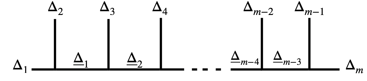
Figure 3: On the above diagram chiral vertex operators with external conformal weights $\boldsymbol{\Delta}:=\left\{\Delta_{1},\ldots,\Delta_{m}\right\}$ have the following locations, $V_{\Delta_{1}}$ is at $x_{0}=0$, $V_{\Delta_{m-2}}$ is at $x_{m-3}$, $V_{\Delta_{m-1}}$ is at $x_{m-2}=1$ and $V_{\Delta_{m}}$ is at $x_{m-1}=\infty$.

Again, the identity (65) is fulfilled when certain relationships between parameters take place, namely,

$$\Delta_{i} = \frac{1}{4\beta}\alpha_{i}\left(\alpha_{i}+2-2\beta\right),\quad i=1,\ldots,m-1,$$

$$\Delta_{m} = \frac{1}{4\beta}\left(\alpha_{1}+\ldots+\alpha_{m-1}+2\beta\left(N_{1}+\ldots+N_{m-2}\right)\right)$$

$$\times\;\left(\alpha_{1}+\ldots+\alpha_{m-1}+2\beta\left(N_{1}+\ldots+N_{m-2}\right)+2-2\beta\right),$$

$${\underline{\Delta}}_{i} = \frac{1}{4\beta}\left(\alpha_{1}+\ldots+\alpha_{i+1}+2\beta\left(N_{1}+\ldots+N_{i}\right)\right)$$

$$\times\;\left(\alpha_{1}+\ldots+\alpha_{i+1}+2\beta\left(N_{1}+\ldots+N_{i}\right)+2-2\beta\right),$$

$$c = 1-6\left(\sqrt{\beta}-\frac{1}{\sqrt{\beta}}\right)^{2}$$

or

$$\Delta_{i} = \hat{\alpha}_{i}\left(\hat{\alpha}_{i}+\frac{1}{b}-b\right),\quad i=1,\ldots,m-1,$$

$$\Delta_{m} = \left(b\left(N_{1}+\ldots+N_{m-2}\right)+\hat{\alpha}_{1}+\ldots+\hat{\alpha}_{m-1}\right)$$

$$\times\;\left(b\left(N_{1}+\ldots+N_{m-2}\right)+\hat{\alpha}_{1}+\ldots+\hat{\alpha}_{m-1}+\frac{1}{b}-b\right),$$

$${\underline{\Delta}}_{p} = \left(b\left(N_{1}+\ldots+N_{p}\right)+\hat{\alpha}_{1}+\ldots+\hat{\alpha}_{p+1}\right)$$

$$\times\;\left(b\left(N_{1}+\ldots+N_{p}\right)+\hat{\alpha}_{1}+\ldots+\hat{\alpha}_{p+1}+\frac{1}{b}-b\right),$$

$$p=1,\ldots,m-3,$$

$$c = 1-6\left(b-\frac{1}{b}\right)^{2}.$$ (69)

As in the four-point case there are two ways to calculate the asymptotic behaviour of ${\cal Z}_{\rm DF}(\boldsymbol{\alpha},{\bf N},b^{2}\,|\,{\bf q})$ with $\boldsymbol{\alpha}:=\left\{2b^{2}\eta_{1},\ldots,2b^{2}\eta_{m-1}\right\}$ for $b\to\infty$. Repeating the same calculation steps as in the previous subsection one gets in the multi-point case an extension of the conjectured relation (64). We formulate this result below.

1. Let us introduce

   • the “action”

     $$W\left(\,\cdot\,|\,{\bf x}({\bf q}),{\bf u}\right) := -2\sum\limits_{\mu<\nu}\log(u_{\nu}-u_{\mu})$$ (70)

     $$- \sum\limits_{\mu=1}^{N_{1}+\ldots+N_{m-2}}\left[\sum\limits_{r=0}^{m-2}2\eta_{r+1}\log\left(u_{\mu}-x_{r}({\bf q})\right)\right],$$

     where ${\bf x}:=\left\{x_{0}=0,x_{1},\ldots,x_{m-3},x_{m-2}=1\right\}$, ${\bf u}:=\left\{u_{1},\ldots,u_{N=N_{1}+\ldots+N_{m-2}}\right\}$ and the symbol $x_{r}({\bf q})$ means that each $x_{r}$, $r=0,\ldots,m-2$ is replaced with corresponding $q$’s, in accordance with (66) and $x_{0}=q_{0}=0$, $x_{m-2}=q_{m-2}=1$;

   • the critical value $W\left(\,\cdot\,|\,{\bf x}({\bf q}),{\bf u}^{\rm c}\right)$ of (70), i.e., the function (70) evaluated on the stationary solution ${\bf u}^{\rm c}:=\left\{u_{1}^{\rm c},\ldots,u_{N=N_{1}+\ldots+N_{m-2}}^{\rm c}\right\}$ of the saddle point equations:

     $$\frac{\partial W\left(\,\cdot\,|\,{\bf x}({\bf q}),{\bf u}\right)}{\partial u_{\mu}}\;=\;0\,\;\;\Leftrightarrow\;\;\sum\limits_{r=0}^{m-2}\frac{2\eta_{r+1}}{u_{\mu}-x_{r}({\bf q})}+\sum\limits_{\nu\neq\mu}^{N}\frac{2}{u_{\mu}-u_{\nu}}\;=\;0,$$ (71)

     $$\forall\;\mu=1,\ldots,N=N_{1}+\ldots+N_{m-2}.$$

2. Let ${\sf S}_{N}(\cdot,\cdot)$ denotes an exponent in the large $\beta$ asymptotic (58) of the structure constant (50) given by (LABEL:SNcl).

3. Let ${\hat{f}}(\boldsymbol{\delta},\underline{\boldsymbol{\delta}}\,|\,{\bf q})$ be a series part of the $m$-point classical Virasoro block in the “comb” channel, i.e.,

   $${\hat{f}}(\boldsymbol{\delta},\underline{\boldsymbol{\delta}}\,|\,{\bf q})\;=\;\lim\limits_{b\to\infty}\frac{1}{b^{2}}\log{\sf B}\!\left(\boldsymbol{\Delta},\underline{\boldsymbol{\Delta}},c\,|\,{\bf q}\right),$$ (72)

   where

   • the parameters $\boldsymbol{\Delta}$, $\underline{\boldsymbol{\Delta}}$, $c$ of the quantum block ${\sf B}\!\left(\boldsymbol{\Delta},\underline{\boldsymbol{\Delta}},c\,|\,{\bf q}\right)$ are given by (3.2);

   • the parameters of the classical block are $\boldsymbol{\delta}:=\left\{\delta_{1},\ldots,\delta_{m}\right\}$, $\underline{\boldsymbol{\delta}}:=\left\{\underline{\delta}_{1},\ldots,\underline{\delta}_{m-3}\right\}$,

     $$\delta_{i} = \lim\limits_{b\to\infty}\frac{1}{b^{2}}\Delta_{i}=\eta_{i}\left(\eta_{i}-1\right),\quad i=1,\ldots,m-1,$$ (73)

     $$\delta_{m} = \lim\limits_{b\to\infty}\frac{1}{b^{2}}\Delta_{m}=\left(N_{1}+\ldots+N_{m-2}+\eta_{1}+\ldots+\eta_{m-1}\right)$$ (74)

     $$\hskip 51.21504pt\times\left(N_{1}+\ldots+N_{m-2}+\eta_{1}+\ldots+\eta_{m-1}-1\right),$$

     $$\underline{\delta}_{p} = \lim\limits_{b\to\infty}\frac{1}{b^{2}}\underline{\Delta}_{p}=\left(N_{1}+\ldots+N_{p}+\eta_{1}+\ldots+\eta_{p+1}\right)$$ (75)

     $$\hskip 51.21504pt\times\left(N_{1}+\ldots+N_{p}+\eta_{1}+\ldots+\eta_{p+1}-1\right),$$

     $$\quad p=1,\ldots,m-3.$$

4. We conjecture that

   $${\hat{f}}(\boldsymbol{\delta},\underline{\boldsymbol{\delta}}\,|\,{\bf q}) = -W\left(\,\cdot\,|\,{\bf x}({\bf q}),{\bf u}^{\rm c}\right)+\sum\limits_{\mu<\nu}2\eta_{\mu}\eta_{\nu}\log(x_{\nu}({\bf q})-x_{\mu}({\bf q}))$$ (76)

   $$-\Big{(}{\sf S}_{N_{1}}(2\eta_{1},2\eta_{2})+{\sf S}_{N_{2}}(\underline{\delta}_{1},2\eta_{3})+\ldots+{\sf S}_{N_{m-2}}(\underline{\delta}_{m-3},2\eta_{m-1})\Big{)}$$

   $$-\sum\limits_{i=1}^{m-3}(\underline{\delta}_{i}-\delta_{1}-\ldots-{\delta}_{i+1})\log q_{i}.$$

The statement is that the part ${\hat{f}}(\boldsymbol{\delta},\underline{\boldsymbol{\delta}}\,|\,{\bf q})$ of the $m$-point classical Virasoro block given by the series in variables $q_{1},\ldots,q_{m-3}$, which is calculable order by order from the quantum block expansion via (72), can be summed up to the r.h.s. of eq. (76). On the r.h.s. the contributions are: ($a$) the “on-shell action” $W\left(\,\cdot\,|\,{\bf x}({\bf q}),{\bf u}^{\rm c}\right)$; ($b$) the exponent ${\sf S}_{N_{1}}+{\sf S}_{N_{2}}+\ldots+{\sf S}_{N_{m-2}}$ in the “classical asymptotic” of $C_{\rm DF}$, where this time $C_{\rm DF}$ is given by (68); ($c$) the classical limit of the prefactor $q_{1}^{{\rm deg}_{1}}\ldots q_{m-3}^{{\rm deg}_{m-3}}$.

4 Richardson and Gaudin models

4.1 Richardson’s solution

The Hamiltonian (7) was studied by Richardson long ago with intent to be used in nuclear physics. $\hat{\rm H}_{\rm rBCS}$ can be written in terms of the so-called “hard-core” boson operators $b_{j}^{\dagger}=c_{j+}^{\dagger}c_{j-}^{\dagger}$ and $b_{j}=c_{j-}c_{j+}$ which create, annihilate fermion pairs, respectively and obey the following commutation rules $\big{[}b_{j},b_{j^{\prime}}^{\dagger}\big{]}=\delta_{j,j^{\prime}}(1-2\hat{\rm N}_{j})$, $\hat{\rm N}_{j}=b_{j}^{\dagger}\,b_{j}$. The reduced BCS Hamiltonian rewritten in terms of these operators reads as follows

$$\hat{\rm H}_{\rm rBCS}=\sum\limits_{j}2\varepsilon_{j}b_{j}^{\dagger}b_{j}-gd\sum\limits_{j,j^{\prime}}b_{j}^{\dagger}b_{j^{\prime}}.$$ (77)

Sums in (77) run over a set of doubly degenerate energy levels with energies $\varepsilon_{j}$, $j=1,\ldots,\Omega$. In the 1960s Richardson exactly solved an eigenvalue problem for (77) through the Bethe ansatz R1 ; RS ; RS2 . (For a pedagogical introduction to the Richardson solution, see vonDelft:1999si .) Specifically, Richardson proposed an ansatz for an exact eigenstate of the Hamiltonian (77), namely,

$$|\,{N}\,\rangle=\prod\limits_{\nu=1}^{N}B^{\dagger}_{\nu}|\,{0}\,\rangle\;,$$

where the pair operators $B^{\dagger}_{\nu}$ have the form appropriate to the solution of the one-pair problem, i.e.,

$$B^{\dagger}_{\nu}=\sum\limits_{j=1}^{\Omega}\frac{b^{\dagger}_{j}}{2\varepsilon_{j}-u_{\nu}}\;.$$

Here every energy level is either empty or occupied by a pair of fermions. The quantities $u_{\nu}$ are pair energies. They are understood as auxiliary parameters which are then chosen to fulfill the eigenvalue equation

$$\hat{\rm H}_{\rm rBCS}\,|\,{N}\,\rangle={\rm E}_{\rm rBCS}(N)\,|\,{N}\,\rangle\;,$$ (78)

where ${\rm E}_{\rm rBCS}(N)\!=\!\sum_{\nu=1}^{N}u_{\nu}$. Indeed, the state $|\,{N}\,\rangle$ is an eigenstate of the pairing Hamiltonian (77) if the $N$ pair energies $u_{\nu}$ are, complex in general, solutions of the (Bethe ansatz) equations:

$$\frac{1}{gd}+\sum\limits_{i=1}^{\Omega}\frac{1}{u_{\nu}-z_{i}}=\sum\limits_{\mu\neq\nu}^{N}\frac{2}{u_{\nu}-u_{\mu}}\;\;\;\;{\rm for}\;\;\nu=1,\ldots,N,$$ (79)

where $z_{i}=2\varepsilon_{i}$. (For a derivation of eqs. (79) using a commutator technique, see vonDelft:1999si .) The ground state of the system is given by the solution of eqs. (79) which gives the lowest value of ${\rm E}_{\rm rBCS}(N)$. The normalized state $|\,{N}\,\rangle$ can be written in the following form

$$|\,{N}\,\rangle=\frac{C}{\sqrt{N!}}\sum\limits_{j_{1},\ldots,j_{N}}\psi(j_{1},\ldots,j_{N})b^{\dagger}_{j_{1}}\ldots b^{\dagger}_{j_{N}}|\,{0}\,\rangle.$$ (80)

In (80) the normalization constant $C$ is determined by the condition $\langle\,{N}\,|\,{N}\,\rangle\!=\!1$ while $\psi(j_{1},\ldots,j_{N})$ is the Richardson wave function of the form

$$\psi^{\rm R}(j_{1},\ldots,j_{N})=\sum\limits_{\mathcal{P}}\prod\limits_{k=1}^{N}\frac{1}{z_{j_{k}}-u_{{\cal P}_{k}}}.$$ (81)

The sum in (81) runs over all permutations $\mathcal{P}$ of $1,\ldots,N$.

There is a connection between the Richardson (reduced BCS) model and a class of integrable spin models obtained by Gaudin Gaudin1 ; Gaudin2 . In 1976 Gaudin proposed the so-called rational, trigonometric and elliptic integrable models based on sets of certain commuting Hamiltonians. The simplest model in this family it is the rational model which is defined by a collection of Hamiltonians of the form

$$\hat{\mathrm{H}}_{{\rm G},i} = \sum\limits_{j\neq i}^{\Omega}\frac{1}{\varepsilon_{i}-\varepsilon_{j}}\left[{\rm t}_{i}^{0}{\rm t}_{j}^{0}+\frac{1}{2}\left({\rm t}_{i}^{+}{\rm t}_{j}^{-}+{\rm t}_{i}^{-}{\rm t}_{j}^{+}\right)\right]$$ (82)

$$=: \sum\limits_{j\neq i}^{\Omega}\frac{{\bf t}_{i}\cdot{\bf t}_{j}}{\varepsilon_{i}-\varepsilon_{j}}.$$

$\hat{\mathrm{H}}_{{\rm G},i}$ describe a system of interacting spins labeled by $i=1,\ldots,\Omega$. Each separate spin corresponds to a spin-$\frac{1}{2}$ realization of the $\mathfrak{su}(2)$ algebra generated by ${\rm t}^{0}$, ${\rm t}^{+}$, ${\rm t}^{-}$. Interestingly, the spin-$\frac{1}{2}$ generators can be written in terms of the hard-core boson operators, i.e., ${\rm t}_{j}^{+}=b_{j}^{+}$, ${\rm t}_{j}^{-}=b_{j}$, ${\rm t}_{j}^{0}=\frac{1}{2}-\hat{\rm N}_{j}$. Therefore, the Gaudin Hamiltonians $\hat{\mathrm{H}}_{{\rm G},i}$ can be diagonalized by means of the Richardson method. As before the energy eigenvalue is given by ${\rm E}_{{\rm G},i}(N)=\sum_{\nu=1}^{N}u_{\nu}$, but this time the parameters $u_{\nu}$ satisfy

$$\sum\limits_{j=1}^{\Omega}\frac{1}{u_{\nu}-z_{j}} = \sum\limits_{\mu\neq\nu}^{N}\frac{2}{u_{\nu}-u_{\mu}}\;\;\;\;{\rm for}\;\;\nu=1,\ldots,N.$$ (83)

Eqs. (83) are nothing but the Richardson eqs. (79) in the limit $g\longrightarrow\infty$.

In 1997 Cambiagio, Rivas and Saraceno (CRS) Cambiaggio:1997vz found that conserved charges of the Richardson–BCS model, i.e., mutually commuting operators $\hat{\rm R}_{i}$ which commute with the reduced BCS Hamiltonian (77), are given in terms of the rational Gaudin Hamiltonians:

$$\hat{\rm R}_{i} = -{\rm t}_{i}^{0}-gd\,\hat{\mathrm{H}}_{{\rm G},i}$$ (84)

$$= -{\rm t}_{i}^{0}-gd\sum\limits_{j\neq i}^{\Omega}\frac{{\bf t}_{i}\cdot{\bf t}_{j}}{\varepsilon_{i}-\varepsilon_{j}},\;\;\;\;\;\;\;\;i=1,\ldots,\Omega.$$

The quantum integrals of motion (84) itself can be seen as a set of commuting Hamiltonians. These are famous Gaudin magnets known also as the central spin model (cf. Claeys:2018zwo and refs therein). The Gaudin magnets play a crucial role in the study of integrable spin models and their connections with 2d CFT, see for instance Babu ; BabuFlume . Moreover, there exist several examples of the integrable (time-dependent) Hamiltonians, relevant for concrete physical applications, which can be reduced to the Gaudin magnets, and integrability of which is determined by the celebrated Knizhnik–Zamolodchikov equation, cf. eg. Yuzbashyan:2018gbu .

The fact that operators $\hat{\rm R}_{i}$ commute with $\hat{\rm H}_{\rm rBCS}$ implies that $\hat{\rm H}_{\rm rBCS}$ can be expressed in terms of $\hat{\rm R}_{i}$, i.e.,

$$\hat{\rm H}_{\rm rBCS}\;=\;\hat{\rm H}_{\rm XY}+\sum\limits_{j=1}^{\Omega}\varepsilon_{j}+gd\left(\tfrac{1}{2}\Omega-N\right),$$ (85)

where

$$\hat{\rm H}_{\rm XY}\;=\;\sum\limits_{j=1}^{\Omega}2\varepsilon_{j}\hat{\rm R}_{j}+gd\Big{(}\sum\limits_{j=1}^{\Omega}\hat{\rm R}_{j}\Big{)}^{2}-\frac{3}{4}gd\,\Omega,$$ (86)

cf. Sierra:1999mp ; Cambiaggio:1997vz . The intermediate step that leads to (85)-(86) is that the operator $\hat{\rm H}_{\rm XY}$ can be expressed as a spin chain Hamiltonian,

$$\hat{\rm H}_{\rm XY}\;=\;-\sum\limits_{j=1}^{\Omega}2\varepsilon_{j}{\rm t}^{0}_{j}-\frac{gd}{2}\left({\rm T}^{+}{\rm T}^{-}+{\rm T}^{-}{\rm T}^{+}\right).$$ (87)

The matrices ${\rm T}^{a}=\sum_{j=1}^{\Omega}{\rm t}_{j}^{a}$, $a\in\{0,+,-\}$ satisfy the ${\mathfrak{su}(2)}$ algebra $\left[{\rm T}^{a},{\rm T}^{b}\right]=f_{c}^{ab}\,{\rm T}^{b}$, where

$$f_{\,+}^{\,+\,0}=f_{-}^{\,0\,-}=-1\,,\quad f_{0}^{\,+\,-}=2\,.$$ (88)

The Casimir of that algebra is given by ${\bf T}\cdot{\bf T}={\rm T}^{0}{\rm T}^{0}+\frac{1}{2}({\rm T}^{+}{\rm T}^{-}+{\rm T}^{-}{\rm T}^{+})$. Eqs. (85) and (86) open a possibility to calculate eigenvalues of quantum integrals of motion $\hat{\rm R}_{i}$ by solving them with respect to $\hat{\rm R}_{i}$. Unluckily, CRS did not compute the eigenvalues of $\hat{\rm R}_{i}$. Perhaps, they didn’t know about the Richardson solution.

In fact, for a long time Richardson results were not assimilated by the scientific community until the end of the 20th century, when it was realized that the Richardson model describes pairing of time-reversed electrons in metalic mesoscopic grains. On this new wave of interest in the Richardson solution more novel ideas sailed out. In particular, in those days Sierra proposed in the aforementioned paper Sierra:1999mp a link between 2d CFT and the exact solution, and integrability of the reduced BCS model. As was explained, for example, in Sierra:2001cx there were several motivations that led to the formulation of such links. One of them was the so-called electrostatic analogy mentioned in the introduction.

Indeed, the Richardson equations (79) can be interpreted within a two-dimensional electrostatic picture. Let us consider a set of $\Omega$ charges with charge $q=-1$ fixed at the positions $z_{i}=2\epsilon_{i}$ on the real axis and an uniform field parallel to this axis with strength $-\frac{1}{gd}$. The task is to find equilibrium positions of $N$ charges with charge $q=+2$ at positions $u_{\nu}$ subject to their mutual repulsion and an attraction wit $\Omega$ charges with $q=-1$, and an action of the uniform field. (The constant electric field is absent in the Gaudin model.) The electrostatic potential is given by $U+\bar{U}$, where the holomorphic part reads as follows

$$U({\bf z},{\bf u}) = -\sum\limits_{i<j}^{\Omega}\log(z_{i}-z_{j})-4\sum\limits_{\nu<\mu}^{N}\log(u_{\nu}-u_{\mu})$$ (89)

$$+ 2\sum\limits_{i=1}^{\Omega}\sum\limits_{\nu=1}^{N}\log(z_{i}-u_{\mu})+\frac{1}{gd}\Big{(}-\sum\limits_{i=1}^{\Omega}z_{i}+2\sum\limits_{\nu=1}^{N}u_{\nu}\Big{)}\,.$$

Here ${\bf z}:=\{z_{1},\ldots,z_{\Omega}\}$ and ${\bf u}:=\{u_{1},\ldots,u_{N}\}$. Therefore, eqs. (79) are nothing but the equilibrium conditions:

$$\frac{\partial U({\bf z},{\bf u})}{\partial u_{\nu}}=0\,,\quad\quad\nu=1,\ldots,N\;.$$ (90)

As already mentioned, the electrostatic picture can be immersed in conformal field theory. The relevant CFT here is given by the $\widehat{\mathfrak{su}(2)}_{k}$ WZW model in the so-called critical level limit $k\longrightarrow-2$. This embedding led to a new result, namely, Sierra using CFT methods found closed expression for eigenvaluse of conserved charges (84), i.e.,

$$\lambda_{i} = \frac{gd}{2}\frac{\partial U({\bf z},{\bf u}^{\sf c})}{\partial z_{i}}\Big{|}_{z_{i}=2\varepsilon_{i}}$$ (91)

$$= -\frac{1}{2}+gd\left(\sum\limits_{\nu=1}^{N}\frac{1}{2\varepsilon_{i}-u_{\nu}^{\sf c}}-\frac{1}{4}\sum\limits_{j\neq i}^{\Omega}\frac{1}{\varepsilon_{i}-\varepsilon_{j}}\right).$$

The quantity $U({\bf z},{\bf u}^{\sf c})\equiv U_{\sf c}$ in eq. (91) above is the critical value of the potential (89), i.e., $U({\bf z},{\bf u})$ evaluated on the solution ${\bf u}^{\sf c}:=\left\{u_{1}^{\sf c},\ldots,u_{N}^{\sf c}\right\}$ of the Richardson equations (79). We review a derivation of eq. (91) in subsection 4.3. Before that we will briefly recall the conformal field theory construction presented in Sierra:1999mp (see also Sierra:2001cx ).

4.2 Embedding in conformal field theory

To realize the Richardson solution within 2d CFT and derive expression for eigenvalues of CRS conserved charges Sierra proposed to consider a perturbed affine conformal block

$$\psi^{\rm CG}_{\bf m}({\bf z}):=\left\langle{\sf V}_{gd}\Phi_{m_{1}}^{\frac{1}{2}}(z_{1})\ldots\Phi_{m_{\Omega}}^{\frac{1}{2}}(z_{\Omega})\tilde{\Phi}_{j_{\Omega+1}}^{j_{\Omega+1}}(\infty)\oint\limits_{C_{1}}{\rm d}u_{1}{\sf S}(u_{1})\ldots\oint\limits_{C_{N}}{\rm d}u_{N}{\sf S}(u_{N})\right\rangle$$ (92)

which contains

• the $\widehat{\mathfrak{su}(2)}_{k}$ WZW chiral primary fields in a free field realization:

  $$\Phi_{m}^{j}(z)=\left(\gamma(z)\right)^{j-m}V_{\alpha}(z)\,,\quad\alpha=(k+2)^{-\frac{1}{2}}j=-2\alpha_{0}j\,$$

  $$\Delta_{\alpha}=\alpha(\alpha-2\alpha_{0})=\frac{j(j+1)}{k+2};$$ (93)

• WZW screening charges:

  $${\sf Q}=\oint\limits_{C}\frac{{\rm d}u}{2\pi i}\,{\sf S}(u)\,,\quad\quad{\sf S}(u)=\beta(u)V_{2\alpha_{0}}(u)\,;$$

• the operator

  $${\sf V}_{gd}=\exp\left(-\frac{i\alpha_{0}}{gd}\oint\limits_{C_{g}}{\rm d}zz\partial_{z}\phi(z)\right),$$

  which breaks conformal invariance.

Within this realization to every energy level $z_{i}=2\varepsilon_{i}$ is associated the field $\Phi_{m_{i}}^{j}(z_{i})$ with the “spin” $j=\frac{1}{2}$ and the “third component” $m_{i}=\frac{1}{2}$ (or $m_{i}=-\frac{1}{2}$) if the corresponding energy level is empty (or occupied) by a pair of fermions. Integration variables $u_{\nu}$ in screening operators correspond to Richardson parameters. The operator ${\sf V}_{gd}$ implements the coupling $gd$ and is a source of the term $\frac{1}{gd}$ in the Richardson equations. In the next subsection, following Sierra:1999mp , we spell out how this idea works, i.e., how this construction is related to the Richardson solution and how it solves eigenproblems for (84).

4.3 Knizhnik–Zamolodchikov equation and integrability

In CFT framework the integrability of the Richardson model is determined by the Knizhnik–Zamolodchikov (KZ) equation,

$$\left(\kappa\partial_{z_{i}}-\sum\limits_{j\neq i}^{\Omega+1}\frac{{\bf t}_{i}\cdot{\bf t}_{j}}{z_{i}-z_{j}}\right)\Psi^{\rm WZW}(z_{1},\ldots,z_{\Omega+1})\;=\;0\,,$$ (94)

which is obeyed by the $\widehat{\mathfrak{su}(2)}_{k}$ WZW conformal block $\Psi^{\rm WZW}(z_{1},\ldots,z_{\Omega+1})$. The coupling constant $\kappa$ in eq. (94) is

$$\kappa\;=\;\frac{(k+2)}{2}\,,$$ (95)

where $k$ is the level of the Kac–Moody algebra of the WZW model. Here, ${\bf t}_{i}$ are the $\mathfrak{su}(2)$ matrices in the $j_{i}$ representation acting at the $i$-th site. Let us observe that for $z_{\Omega+1}\longrightarrow\infty$ the term $({\bf t}_{i}\cdot{\bf t}_{\Omega+1})/(z_{i}-z_{\Omega+1})$ in (94) equals zero. Therefore, in such a case one can use the identity

$$\frac{1}{2gd}\hat{\rm R}_{i}+\frac{1}{2gd}{\rm t}_{i}^{0}=-\sum\limits_{j\neq i}^{\Omega}\frac{{\bf t}_{i}\cdot{\bf t}_{j}}{z_{i}-z_{j}},$$

which follows from the form of $\hat{\rm R}_{i}$ for $z_{j}=2\varepsilon_{j}$, and the KZ equation (94) rewrite to the following form

$$\left(\kappa\partial_{z_{i}}+\frac{1}{2gd}\hat{\rm R}_{i}+\frac{1}{2gd}{\rm t}_{i}^{0}\right)\Psi^{\rm WZW}(z_{1},\ldots,z_{\Omega},\infty)=0.$$ (96)

Let us define a new function $\Psi$ related to $\Psi^{\rm WZW}$ by

$$\Psi^{\rm WZW}=\exp\left(\frac{1}{2gd\kappa}\hat{\rm H}_{\rm XY}\right)\Psi.$$ (97)

Elementary calculations yield

$$\kappa\partial_{z_{i}}\Psi^{\rm WZW} = \exp\left(\frac{1}{2gd\kappa}\hat{\rm H}_{\rm XY}\right)$$

$$\times \left[\frac{1}{2gd}\left(\partial_{z_{i}}\hat{\rm H}_{\rm XY}\right)\Psi+\kappa\partial_{z_{i}}\Psi\right].$$

The operators $\hat{\rm R}_{i}$ and $\hat{\rm H}_{\rm XY}$ commute therefore on can write

$$\hat{\rm R}_{i}\exp\left(\frac{1}{2gd\kappa}\hat{\rm H}_{\rm XY}\right)=\exp\left(\frac{1}{2gd\kappa}\hat{\rm H}_{\rm XY}\right)\hat{\rm R}_{i}.$$

Using these two identities one gets from eq. $(\ref{KZEsu2II})$ the equation for $\Psi$,

$$\left(\kappa\partial_{z_{i}}+\frac{1}{2gd}\partial_{z_{i}}\hat{\rm H}_{\rm XY}+\frac{1}{2gd}\hat{\rm R}_{i}+\frac{1}{2gd}{\rm t}_{i}^{0}\right)\Psi=0.$$

Let us observe that $\partial_{z_{i}}\hat{\rm H}_{\rm XY}=-{\rm t}_{i}^{0}$ as it follows from (87) for $z_{j}=2\varepsilon_{j}$. Therefore, we have

$$\frac{1}{2gd}\hat{\rm R}_{i}\Psi=-\kappa\partial_{z_{i}}\Psi.$$ (98)

Eq. (98) is completely equivalent to the KZ equation and has been obtained in Sierra:1999mp . Our aim now is to calculate its classical limit $c\longrightarrow\infty\;\iff\;\alpha_{0}\longrightarrow\infty$. We will see that in the limit $\alpha_{0}\longrightarrow\infty$ eq. (98) is nothing but the eigenvalue problem for conserved charges $\hat{\rm R}_{i}$. This result we summarize in the following lemma.

If the function $\Psi({\bf z})$, ${\bf z}:=\{z_{1},\ldots,z_{\Omega}\}$ in (98) has the following asymptotical behaviour in the limit $\alpha_{0}\longrightarrow\infty$,

$$\Psi({\bf z})\sim\tilde{\psi}({\bf z})\,{\rm e}^{-\alpha_{0}^{2}U({\bf z},{\bf u}^{\sf c})},$$ (99)

where $\tilde{\psi}({\bf z})$ has the “lightness” property

$$\lim\limits_{\kappa\to 0}\kappa\partial_{z_{i}}\tilde{\psi}({\bf z})\;=\;0$$ (100)

then the function $\tilde{\psi}({\bf z})$ solves the eigenvalue problem for the Richardson model conserved charges,

$$\hat{\rm R}_{i}\tilde{\psi}\;=\;\lambda_{i}\tilde{\psi}$$ (101)

with the eigenvalues $\lambda_{i}$ of integrals of motion given by

$$\lambda_{i}\;=\;\frac{gd}{2}\frac{\partial U_{\sf c}}{\partial z_{i}}\;.$$ (102)

Indeed, a substitution of (99) into eq. (98) gives

$$\frac{1}{2gd}\hat{\rm R}_{i}\tilde{\psi}+\kappa\partial_{z_{i}}\tilde{\psi}-\alpha_{0}^{2}\kappa(\partial_{z_{i}}U_{\sf c})\tilde{\psi}\;=\;0.$$ (103)

The central charge $c$ in the case under consideration is parametrized in terms of the background charge $\alpha_{0}$ and is related to $k$ — the level of the Kac–Moody algebra:

$$c=3-12\alpha_{0}^{2}=\frac{3k}{k+2}.$$

In addition, $k$ is related to the coupling $\kappa$ in the KZ equation via (95). So the large central charge limit $c\longrightarrow\infty$ corresponds to $\alpha_{0}\longrightarrow\infty$ and to the critical level limit $k\longrightarrow-2$, and finally to $\kappa\longrightarrow 0$. Knowing that one can find that

$$\alpha_{0}^{2}\kappa = \frac{\alpha_{0}^{2}}{2}2\kappa=\frac{\alpha_{0}^{2}}{2}(k+2)=\frac{\alpha_{0}^{2}}{2}\frac{3k}{3-12\alpha_{0}^{2}}$$ (104)

$$= \frac{3k}{\frac{6}{\alpha_{0}^{2}}-24}\longrightarrow\frac{-6}{-24}=\frac{1}{4}$$

for $\alpha_{0}\longrightarrow\infty$ and simultaneously $k\longrightarrow-2$. Therefore, in the limit $\alpha_{0}\longrightarrow\infty$ taking into account (100) from (103) we obtain $\hat{\rm R}_{i}\tilde{\psi}=\frac{1}{2}gd(\partial_{z_{i}}U_{\sf c})\tilde{\psi}$.

Thus, to solve spectral problems for CRS conserved charges one has to construct the function $\Psi({\bf z})$ related to WZW conformal block via (97) and having the $\alpha_{0}\longrightarrow\infty$ asymptotic of the form (99). This concrete realization of $\Psi({\bf z})$ with required asymptotic behaviour was found in Sierra:1999mp . Precisely, $\Psi({\bf z})$ is nothing but the perturbed WZW block (92). The latter has the asymptotic (99) for $\alpha_{0}\longrightarrow\infty$. Indeed, from (92) one gets

$$\psi^{\rm CG}_{\bf m}({\bf z})\;=\;\oint\limits_{C_{1}}{\rm d}u_{1}\ldots\oint\limits_{C_{N}}{\rm d}u_{N}\,\psi^{\beta\gamma}_{\bf m}({\bf z},{\bf u}){\rm e}^{-\alpha_{0}^{2}\,U({\bf z},{\bf u})}\;,$$

where

$$\psi^{\beta\gamma}_{\bf m}({\bf z},{\bf u})\;=\;\left\langle\prod\limits_{i=1}^{\Omega}\gamma^{\frac{1}{2}-m_{i}}(z_{i})\prod\limits_{\nu=1}^{N}\beta(u_{\nu})\beta^{s+2j_{\Omega+1}}(\infty)\gamma^{2j_{\Omega+1}}(\infty)\right\rangle\;$$

and $U({\bf z},{\bf u})$ is the potential (89). In the limit $\alpha_{0}\longrightarrow\infty$ the above multiple contour integral can be calculated using the saddle point method. Recall, the stationary solutions of $U$ are given by the solutions of the Richardson equation. As a result one gets (99), where $\tilde{\psi}({\bf z})=\psi^{\beta\gamma}_{\bf m}({\bf z},{\bf u}^{\sf c})$ is the Richardson wave function and $U_{\sf c}\equiv U({\bf z},{\bf u}^{\sf c})$ is the “on-shell” potential appearing in (91). $U_{\sf c}$ is named the Coulomb energy in Sierra:1999mp .

One sees that the Coulomb energy $U_{\sf c}$ and eigenvalues (91) of CRS conserved charges depend on the Richardson parameters ${\bf u}^{\sf c}:=\left\{u_{1}^{\sf c},\ldots,u_{N}^{\sf c}\right\}$. It would be nice to have techniques that allow to find $U_{\sf c}$ without need to solve the Richardson equations. It seems possible to develop such methods. Let us note that $U_{\sf c}$ is an analogue of the “on-shell” action $W(\,\cdot\,|\,\cdot\,,{\bf u}^{\rm c})$ appearing in relations (64) and (76). In the unperturbed case $g\longrightarrow\infty$ corresponding to the rational Gaudin model $U_{\sf c}$ is a direct analogue. Indeed, for $g\longrightarrow\infty$ the VEV (92) is nothing but the WZW block, where an integrand decomposes onto two standard CFT contributions, i.e., some Virasoro block and a chiral function of the $\beta\gamma$ system. So, it is reasonable to expect that $U_{\sf c}$ should be related to the classical limit of some WZW block in unperturbed case and to its “perturbed counterpart” for finite coupling $g$.

5 Concluding remarks

In the present work, exploiting known connections between power series and integral representations of Virasoro conformal blocks (the MMS identities MMS ), we have proposed new expressions (64) and (76) for classical Virasoro blocks. The four-point identity (64) we analyzed numerically in some special case (see appendix C). We observed that for some real solution of the saddle point equations, the real parts of both sides of this relation are almost identical for $x$ in the vicinity of zero. Unfortunately, the imaginary parts of this relationship differ, which may be due to the incompatibility of branches of functions appearing on both sides. A more comprehensive analytical and numerical analysis of these relationships we leave as a topic for further research.

When deriving formulae (64) and (76), we have been inspired by the ideas used in the work Sierra:1999mp . Also this work was our special motivation for this research line. As has been mentioned in the last paragraph of the previous section, identities connecting the classical limit of conformal blocks expansions with the saddle point approximation of Coulomb gas integrals can lead to new computational techniques applicable to the solution of the Richardson and Gaudin models. It seems to be a highly non trivial task to develop such methods for the Richardson model. Here in fact one needs to derive the MMS-type relations for the perturbed WZW block (92). However, this should be achievable for the Gaudin model, where a relevant tool is the (unperturbed) WZW block in a free field representation. Interestingly, it seems that in both cases matrix models tools can help. In particular, the Dijkgraaf–Vafa quasiclassical approach (see e.g. MSh ) and techniques developed in EyMar by Eynard and Marchal should be helpful.

Regardless of the possible applications, the use of matrix models technology in the study of the classical limit of Virasoro and WZW conformal blocks appears promising. This is the topic that we also intend to re-examine soon.

Appendix A Saddle point asymptotics of complex valued integrals

In this appendix we attached a key tool for our calculations, i.e., a steepest descent formula for the $N$-dimensional complex integrals proved by N. Bleistein in the note: “Saddle Point Contribution for an $n$-fold Complex-Valued Integral”.

Let

$${\cal K}_{N}(\omega)\;=\;\int{\rm d}z_{1}\ldots{\rm d}z_{N}f({\bf z})\,{\rm e}^{-\omega\Psi({\bf z})},\quad\quad{\bf z}=\left\{z_{1},\ldots,z_{N}\right\},$$ (105)

where it is assumed that

• the exponent has a simple saddle point in all variables that is

  $$\boldsymbol{\nabla}_{z}\Psi({\bf z})\;=\;\boldsymbol{0},\quad\quad{\bf z}={\bf z}_{\rm sad}:=\left\{z_{1,\rm sad},\ldots,z_{N,\rm sad}\right\};$$ (106)

• the Hessian matrix $\boldsymbol{\Psi}_{N}$, the matrix of second derivatives of $\Psi({\bf z})$, is non-singular at the simple saddle point determined by (106), i.e.,

  $$\det\left(\boldsymbol{\Psi}_{N}\right)\neq 0,\quad\quad\boldsymbol{\Psi}_{N}=\left(\frac{\partial^{2}\Psi}{\partial z_{i}\partial z_{j}}\right)\Big{|}_{{\bf z}={\bf z}_{\rm sad}},\quad\quad i,j=1,2,\ldots,N.$$ (107)

  Then, the leading order asymptotic of ${\cal K}_{N}(\omega)$ for $\omega\to\infty$ is

  $${\cal K}_{N}(\omega)\;\sim\;\left(\frac{2\pi}{\omega}\right)^{\frac{N}{2}}\frac{f({\bf z}_{\rm sad})}{\sqrt{\det\left(\boldsymbol{\Psi}_{N}\right)}}\,{\rm e}^{-\omega\Psi({\bf z}_{\rm sad})}.$$ (108)

Appendix B Asymptotics of Selberg integral

The formula:

$$I_{N}(\lambda_{1},\lambda_{2},\lambda_{3}) := \int\limits_{0}^{1}{\rm d}t_{1}\ldots\int\limits_{0}^{1}{\rm d}t_{N}\prod\limits_{j=1}^{N}t_{j}^{\lambda_{1}}\left(1-t_{j}\right)^{\lambda_{2}}\prod\limits_{1\leq j<i\leq N}\left(t_{i}-t_{j}\right)^{2\lambda_{3}}$$ (109)

$$= \prod\limits_{k=0}^{N-1}\frac{\Gamma(\lambda_{1}+1+k\lambda_{3})\Gamma(\lambda_{2}+1+k\lambda_{3})\Gamma(1+(k+1)\lambda_{3})}{\Gamma(\lambda_{1}+\lambda_{2}+2+(N+k-1)\lambda_{3})\Gamma(1+\lambda_{3})}$$

$$= \prod\limits_{\ell=1}^{N}\frac{\Gamma(\lambda_{1}+1+(\ell-1)\lambda_{3})\Gamma(\lambda_{2}+1+(\ell-1)\lambda_{3})\Gamma(1+\ell\lambda_{3})}{\Gamma(\lambda_{1}+\lambda_{2}+2+(N+\ell-2)\lambda_{3})\Gamma(1+\lambda_{3})},$$

where $0<t_{1}<\ldots<t_{N}<1$, is known as the Selberg integral (see Forr ; Var ). In the case $N=1$ this integral is the Euler beta integral:

$$\int\limits_{0}^{1}t^{\lambda_{1}}(1-t)^{\lambda_{2}}{\rm d}t\;=\;\frac{\Gamma(\lambda_{1}+1)\Gamma(\lambda_{2}+1)}{\Gamma(\lambda_{1}+\lambda_{2}+2)}.$$

Let

$$\lambda_{1}=\frac{\sf a}{\kappa},\quad\lambda_{2}=\frac{\sf b}{\kappa},\quad\lambda_{3}=\frac{\sf c}{\kappa},\quad{\sf a},{\sf b},{\sf c},\kappa>0\quad{\rm and}\quad\kappa\to 0.$$

For the left hand side of (109) the method of steepest descent gives (see appendix A)

$$I_{N}\left(\lambda_{1},\lambda_{2},\lambda_{3}\right)\;\;\sim\;\;(2\pi\kappa)^{\frac{N}{2}}\;\Phi\left(t^{0};\frac{\sf a}{\kappa},\frac{\sf b}{\kappa},\frac{\sf c}{\kappa}\right)\;\left[{\rm Hess}(-S\left(t^{0};{\sf a},{\sf b},{\sf c}\right))\right]^{-\frac{1}{2}}.$$ (110)

Here,

$$\Phi(t;\lambda_{1},\lambda_{2},\lambda_{3})=\prod\limits_{j=1}^{N}t_{j}^{\lambda_{1}}\left(1-t_{j}\right)^{\lambda_{2}}\prod\limits_{1\leq j<i\leq N}\left(t_{i}-t_{j}\right)^{2\lambda_{3}}$$

and

$$S\left(t;{\sf a},{\sf b},{\sf c}\right) = \kappa\log\Phi\left(t;\frac{\sf a}{\kappa},\frac{\sf b}{\kappa},\frac{\sf c}{\kappa}\right)$$

$$= \sum\limits_{j=1}^{N}\left({\sf a}\log t_{j}+{\sf b}\log(1-t_{j})\right)+\sum\limits_{1\leq j<i\leq N}2{\sf c}\log\left(t_{i}-t_{j}\right);$$

$t^{0}$ is the critical point of $S$ in $\left\{t\in\mathbb{R}^{N}\;|\;0<t_{1}<\ldots<t_{N}<1\right\}$ and

$${\rm Hess}(-S) = \det\left(-\frac{\partial^{2}S}{\partial t_{i}\partial t_{j}}\right),$$

$$-\frac{\partial^{2}S}{\partial t_{i}^{2}} = {\sf a}\frac{1}{t_{i}^{2}}+{\sf b}\frac{1}{(t_{i}-1)^{2}}+2{\sf c}\sum\limits_{j\neq i}\frac{1}{(t_{i}-t_{j})^{2}},$$

$$-\frac{\partial^{2}S}{\partial t_{i}\partial t_{j}} = -2{\sf c}\frac{1}{(t_{i}-t_{j})^{2}}.$$

Equations for critical points are

$$\frac{\partial S}{\partial t_{i}}=0\quad\Leftrightarrow\quad\frac{\sf a}{t_{i}}+\frac{\sf b}{t_{i}-1}+\sum\limits_{j\neq i}\frac{2\sf c}{t_{i}-t_{j}}=0,\quad i=1,\ldots,N.$$

Let

$$\lambda_{N}=t^{0}_{1}\ldots t^{0}_{N},\quad\quad\mu_{N}=(1-t^{0}_{1})\ldots(1-t^{0}_{N}),\quad\quad\delta=\prod\limits_{i<j}\left(t^{0}_{i}-t^{0}_{j}\right)^{2}$$

then

$$\Phi\left(t^{0};\frac{\sf a}{\kappa},\frac{\sf b}{\kappa},\frac{\sf c}{\kappa}\right)=\lambda_{N}^{\frac{\sf a}{\kappa}}\cdot\mu_{N}^{\frac{\sf b}{\kappa}}\cdot\delta^{\frac{\sf c}{\kappa}}\quad\Longrightarrow\quad S\left(t^{0};{\sf a},{\sf b},{\sf c}\right)={\sf a}\log\lambda_{N}+{\sf b}\log\mu_{N}+{\sf c}\log\delta.$$

So, the asymptotic (120) takes the form

$$I_{N}\left(\lambda_{1},\lambda_{2},\lambda_{3}\right) \sim \left(\frac{2\pi}{\frac{1}{\kappa}}\right)^{\frac{N}{2}}\;\exp\left[-\frac{1}{\kappa}\left(-S\left(t^{0};{\sf a},{\sf b},{\sf c}\right)\right)\right]$$ (111)

$$\times \left[{\rm Hess}\left(-S\left(t^{0};{\sf a},{\sf b},{\sf c}\right)\right)\right]^{-\frac{1}{2}}.$$

On the other hand one can apply the Stirling formula to the r.h.s. of (109). This calculation has been performed by A. Varchenko in Var , who compared both asymptotics and got an interesting result, i.e., the following formulae:

$$\delta = \prod\limits_{k=0}^{N-1}\frac{(k+1)^{k+1}{\sf c}^{k}({\sf a}+k{\sf c})^{k}({\sf a}+k{\sf c})^{k}}{({\sf a}+{\sf b}+(2N-k-2){\sf c})^{2N-k-2}},$$

$${\rm Hess}\left(-S\left(t^{0};{\sf a},{\sf b},{\sf c}\right)\right) = \prod\limits_{k=0}^{N-1}\frac{({\sf a}+{\sf b}+(2N-k-2){\sf c})^{3}}{({\sf a}+k{\sf c})({\sf b}+k{\sf c})}.$$

The integral (50), namely,

$$C_{N}(b^{2}\rho,b^{2}\omega) = \int\limits_{0}^{1}{\rm d}u_{1}\ldots\int\limits_{0}^{1}{\rm d}u_{N}{\rm e}^{-b^{2}{\sf S}_{N}({\bf u},\rho,\omega)},$$

$${\sf S}_{N}({\bf u},\rho,\omega) = -\sum\limits_{i=1}^{N}\left(\rho\log u_{i}+\omega\log(u_{i}-1)\right)-2\sum\limits_{1\leq i<j\leq N}\log(u_{j}-u_{i}).$$

is nothing but the Selberg integral. The saddle point approximation of $C_{N}(b^{2}\rho,b^{2}\omega)$ for $b\to\infty$ yields the same as above, i.e.,

$$C_{N}(b^{2}\rho,b^{2}\omega)\;\sim\;\left(\frac{2\pi}{b^{2}}\right)^{\frac{N}{2}}\frac{{\rm e}^{-b^{2}{\sf S}_{N}(\rho,\omega)}}{\sqrt{{\rm Hess}({\sf S}_{N}(\rho,\omega))}},$$

where ${\sf S}_{N}(\rho,\omega)\equiv{\sf S}_{N}\left({\bf u}^{\rm c},\rho,\omega\right)$ and ${\bf u}^{\rm c}$ is a solution of critical points eqs.: $\partial{\sf S}_{N}({\bf u},\rho,\omega)/\partial u_{i}=0$, $i=1,\ldots,N$.

As an example and for further uses (see appendix C) let us calculate ${\sf S}_{N}(\rho,\omega)$ in two simplest cases of $N=1$ and $N=2$.

• $N=1$ Here,

  $${\sf S}_{1}(u,\rho,\omega)=-\rho\log u-\omega\log(u-1)=-\rho\log u-\omega\log(1-u)-i\pi\omega$$

  and

  $$C_{1}(b^{2}\rho,b^{2}\omega)=\int\limits_{0}^{1}{\rm d}u\,{\rm e}^{-b^{2}{\sf S}_{1}(u,\rho,\omega)} = {\rm e}^{b^{2}i\pi\omega}\int\limits_{0}^{1}{\rm d}u\,u^{b^{2}\rho}\left(1-u\right)^{b^{2}\omega}$$ (112)

  $$= {\rm e}^{b^{2}i\pi\omega}\frac{\Gamma(b^{2}\rho+1)\Gamma(b^{2}\omega+1)}{\Gamma(b^{2}\rho+b^{2}\omega+2)}.$$

  The saddle point equation takes the form

  $$\frac{\rho}{u}+\frac{\omega}{u-1}\;=\;0$$

  and the solution is

  $$u^{\rm c}(\rho,\omega)=\frac{\rho}{\rho+\omega}.$$

  Therefore,

  $${\sf S}_{1}\left(\rho,\omega\right)\equiv{\sf S}_{1}\left(u^{\rm c}(\rho,\omega),\rho,\omega\right) = -\rho\log\left(\frac{\rho}{\rho+\omega}\right)-\omega\log\left(1-\frac{\rho}{\rho+\omega}\right)-i\pi\omega$$ (113)

  $$= -\rho\log\left(\frac{\rho}{\rho+\omega}\right)-\omega\log\left(\frac{\omega}{\rho+\omega}\right)-i\pi\omega.$$

  and

  $$C_{1}(b^{2}\rho,b^{2}\omega)\sim\left(\frac{2\pi}{b^{2}}\right)^{\frac{1}{2}}\frac{{\rm e}^{-b^{2}{\sf S}_{1}(\rho,\omega)}}{\sqrt{\partial^{2}_{u}{\sf S}_{1}(\rho,\omega)}}.$$

  Applying Stirling’s formula $\Gamma(z)=\sqrt{\frac{2\pi}{z}}\left(\frac{z}{\rm e}\right)^{z}(1+O(1/z))$ to the r.h.s. of (112) one can get the same asymptotical behaviour of $C_{1}(b^{2}\rho,b^{2}\omega)$ for $b\to\infty$, namely,

  $$\frac{\sqrt{2\pi}}{b}O(b^{0})\exp(-b^{2}{\sf S}_{1}(\rho,\omega)).$$

• $N=2$ Here,

  $${\sf S}_{2}({\bf u},\rho,\omega) = -\rho\left(\log u_{1}+\log u_{2}\right)-\omega\left(\log(u_{1}-1)+\log(u_{2}-1)\right)-2\log(u_{2}-u_{1})$$

  and

  $$\frac{\partial{\sf S}_{2}}{\partial u_{1}}=0 \Leftrightarrow \frac{\rho}{u_{1}}+\frac{\omega}{u_{1}-1}+\frac{2}{u_{1}-u_{2}}=0,$$

  $$\frac{\partial{\sf S}_{2}}{\partial u_{2}}=0 \Leftrightarrow \frac{\rho}{u_{2}}+\frac{\omega}{u_{2}-1}+\frac{2}{u_{2}-u_{1}}=0.$$

  The above equations have two pairs of analytical solutions. First,

  $$u_{1}^{\rm c}(\rho,\omega) = \frac{\rho(\rho+\omega+2)-\sqrt{(\rho+1)(\omega+1)(\rho+\omega+1)}+\omega+1}{(\rho+\omega+1)(\rho+\omega+2)},$$

  $$u_{2}^{\rm c}(\rho,\omega) = \frac{\rho(\rho+\omega+2)+\sqrt{(\rho+1)(\omega+1)(\rho+\omega+1)}+\omega+1}{(\rho+\omega+1)(\rho+\omega+2)}$$

  and the second pair, which is a permutation of components of the first. So, to calculate the critical value ${\sf S}_{2}\left({\bf u}^{\rm c},\rho,\omega\right)$ of ${\sf S}_{2}\left({\bf u},\rho,\omega\right)$ we need to evaluate the latter on the critical solutions. For instance,

  $${\sf S}_{2}\left(\rho,\omega\right)\equiv{\sf S}_{2}\left(u_{1}^{\rm c}(\rho,\omega),u_{2}^{\rm c}(\rho,\omega),\rho,\omega\right).$$

Appendix C Numerical checks of the four-point relation

In this appendix we test the conjectured relation (64) numerically in some special cases. Recall, that on the left side of the eq. (64) occurs the $s$-channel classical four-point block on the sphere (cf. eqs. (59)-(60)), i.e.,

$$f(\delta_{1},\ldots,\delta_{4},\underline{\delta}\,|\,x)\;=\;\left(\underline{\delta}-\delta_{1}-\delta_{2}\right)\log x+\hat{f}(\delta_{1},\ldots,\delta_{4},\underline{\delta}\,|\,x).$$ (114)

As already mentioned, the function $\hat{f}(\delta_{1},\ldots,\delta_{4},\underline{\delta}\,|\,x)$ is given by a power series in $x$,

$$\hat{f}(\delta_{1},\ldots,\delta_{4},\underline{\delta}\,|\,x)=\sum\limits_{n=1}^{\infty}x^{n}\hat{f}_{n}(\delta_{1},\ldots,\delta_{4},\underline{\delta}),$$

where coefficients $\hat{f}_{n}(\delta_{1},\ldots\delta_{4},\underline{\delta})$ are calculated directly from the asymptotic behaviour (5) and the power expansion of the quantum block,

$$\sum\limits_{n=1}^{\infty}x^{n}\hat{f}_{n}(\delta_{1},\ldots,\delta_{4},\underline{\delta})=\lim\limits_{b\to\infty}\frac{1}{b^{2}}\log\left(1+\sum_{n=1}^{\infty}x^{n}{\sf B}_{n}\!\left(\Delta_{1},\ldots,\Delta_{4},\underline{\Delta},c\right)\right).$$ (115)

Here, the central charge $c$ is given by (2) and the relation (4) between classical and quantum conformal weights is assumed. It is also reasonable to assume that $0<|x|<1$, as it is dictated by the radial ordering of primary fields in the $s$-channel four-point function. For such $x$ both the quantum and classical four-point blocks are convergent. So, to get $\hat{f}_{n}(\delta_{1},\ldots,\delta_{4},\underline{\delta})$ one needs coefficients of the quantum block. For lower orders of the expansion these coefficients can be easily computed directly from a definition. For instance (cf. MMS ),

$${\sf B}_{1} = \frac{\left(\underline{\Delta}+\Delta_{2}-\Delta_{1}\right)\left(\underline{\Delta}+\Delta_{3}-\Delta_{4}\right)}{2\underline{\Delta}},$$ (116)

$${\sf B}_{2} = \Big{[}\left(\underline{\Delta}-\Delta_{1}+\Delta_{2}\right)\left(\underline{\Delta}-\Delta_{1}+\Delta_{2}+1\right)\left(\underline{\Delta}+\Delta_{3}-\Delta_{4}\right)$$ (117)

$$\left(\underline{\Delta}+\Delta_{3}-\Delta_{4}+1\right)\left(4\underline{\Delta}+\frac{c}{2}\right)-6\underline{\Delta}\left(\underline{\Delta}-\Delta_{1}+2\Delta_{2}\right)$$

$$\left(\underline{\Delta}+\Delta_{3}-\Delta_{4}\right)\left(\underline{\Delta}+\Delta_{3}-\Delta_{4}+1\right)-6\underline{\Delta}\left(\underline{\Delta}-\Delta_{1}+\Delta_{2}\right)$$

$$\left(\underline{\Delta}-\Delta_{1}+\Delta_{2}+1\right)\left(\underline{\Delta}+2\Delta_{3}-\Delta_{4}\right)+4\underline{\Delta}\left(\underline{\Delta}-\Delta_{1}+2\Delta_{2}\right)$$

$$\left(\underline{\Delta}+2\Delta_{3}-\Delta_{4}\right)\left(2\underline{\Delta}+1\right)\Big{]}\Big{[}2\underline{\Delta}\left(2(c-5)\underline{\Delta}+16\underline{\Delta}^{2}+c\right)\Big{]}^{-1}$$

and

$${\sf B}_{3} = \left[2\underline{\Delta}(3\underline{\Delta}^{2}+c\underline{\Delta}-7\underline{\Delta}+2+c)\right]^{-1}$$ (118)

$$\times \Big{[}(\underline{\Delta}+3\Delta_{2}-\Delta_{1})(\underline{\Delta}^{2}+3\underline{\Delta}+2)(\underline{\Delta}+3\Delta_{3}-\Delta_{4})$$

$$- 2(\underline{\Delta}+3\Delta_{2}-\Delta_{1})(\underline{\Delta}+1)(\underline{\Delta}+2\Delta_{3}-\Delta_{4})(\underline{\Delta}+\Delta_{3}-\Delta_{4}+2)$$

$$+ (\underline{\Delta}+3\Delta_{2}-\Delta_{1})(\underline{\Delta}+\Delta_{3}-\Delta_{4})(\underline{\Delta}+\Delta_{3}-\Delta_{4}+1)(\underline{\Delta}+\Delta_{3}-\Delta_{4}+2)$$

$$- 2(\underline{\Delta}+2\Delta_{2}-\Delta_{1})(\underline{\Delta}+\Delta_{2}-\Delta_{1}+2)(\underline{\Delta}+1)(\underline{\Delta}+3\Delta_{3}-\Delta_{4})$$

$$+ (\underline{\Delta}+\Delta_{2}-\Delta_{1})(\underline{\Delta}+\Delta_{2}-\Delta_{1}+1)(\underline{\Delta}+\Delta_{2}-\Delta_{1}+2)(\underline{\Delta}+3\Delta_{3}-\Delta_{4})$$

$$+ 2(\underline{\Delta}+2\Delta_{2}-\Delta_{1})(\underline{\Delta}+\Delta_{2}-\Delta_{1}+2)(6\underline{\Delta}^{3}+9\underline{\Delta}^{2}-9\underline{\Delta}+2c\underline{\Delta}^{2}+3c\underline{\Delta}+c)$$

$$\times (\underline{\Delta}+2\Delta_{3}-\Delta_{4})(\underline{\Delta}+\Delta_{3}-\Delta_{4}+2)\left[16\underline{\Delta}^{2}+2(c-5)\underline{\Delta}+c\right]^{-1}$$

$$- \left[16\underline{\Delta}^{2}+2(c-5)\underline{\Delta}+c\right]^{-1}(\underline{\Delta}+2\Delta_{2}-\Delta_{1})(\underline{\Delta}+\Delta_{2}-\Delta_{1}+2)(9\underline{\Delta}^{2}-7\underline{\Delta}+3c\underline{\Delta}+c)$$

$$\times (\underline{\Delta}+\Delta_{3}-\Delta_{4})(\underline{\Delta}+\Delta_{3}-\Delta_{4}+1)(\underline{\Delta}+\Delta_{3}-\Delta_{4}+2)$$

$$- \left[16\underline{\Delta}^{2}+2(c-5)\underline{\Delta}+c\right]^{-1}(\underline{\Delta}+\Delta_{2}-\Delta_{1})(\underline{\Delta}+\Delta_{2}-\Delta_{1}+1)(\underline{\Delta}+\Delta_{2}-\Delta_{1}+2)$$

$$\times (9\underline{\Delta}^{2}-7\underline{\Delta}+3c\underline{\Delta}+c)(\underline{\Delta}+2\Delta_{3}-\Delta_{4})(\underline{\Delta}+\Delta_{3}-\Delta_{4}+2)$$

$$+ (\underline{\Delta}+\Delta_{2}-\Delta_{1})(\underline{\Delta}+\Delta_{2}-\Delta_{1}+1)(\underline{\Delta}+\Delta_{2}-\Delta_{1}+2)$$

$$\times (\underline{\Delta}+\Delta_{3}-\Delta_{4})(\underline{\Delta}+\Delta_{3}-\Delta_{4}+1)(\underline{\Delta}+\Delta_{3}-\Delta_{4}+2)$$

$$\times \frac{24\underline{\Delta}^{2}-26\underline{\Delta}+11c\underline{\Delta}+8c+c^{2}}{12\left(16\underline{\Delta}^{2}+2(c-5)\underline{\Delta}+c\right)}\Big{]}.$$

For higher orders the calculation of conformal block coefficients by inverting the Gram matrices become very laborious. A more efficient method based on recurrence relations for the coefficients can be used Z1 ; Z2 ; ZZ . Having in hands (116)-(118) one can compute the classical block coefficients expanding the logarithm in (115) into power series and then taking the limit of each term separately. For $n=1,2,3$ one finds:

$$\hat{f}_{1} = \frac{\left(\underline{\delta}-\delta_{1}+\delta_{2}\right)\left(\underline{\delta}+\delta_{3}-\delta_{4}\right)}{2\underline{\delta}},$$

$$\hat{f}_{2} = \Big{[}13\underline{\delta}^{5}+\left(-14\delta_{1}+18\delta_{2}+18\delta_{3}-14\delta_{4}-9\right)\underline{\delta}^{4}$$

$$+ (\delta_{1}^{2}-2\left(\delta_{2}+6\delta_{3}-10\delta_{4}-6\right)\delta_{1}+\delta_{2}^{2}+\delta_{3}^{2}+\delta_{4}^{2}$$

$$- 12\delta_{3}+4\delta_{2}\left(5\delta_{3}-3\delta_{4}-3\right)-2\delta_{3}\delta_{4}+12\delta_{4})\underline{\delta}^{3}$$

$$- 3(\left(2\delta_{3}+2\delta_{4}+1\right)\delta_{1}^{2}-2(-\delta_{3}^{2}+2\left(\delta_{4}+1\right)\delta_{3}-\delta_{4}\left(\delta_{4}+2\right)$$

$$+ \delta_{2}\left(2\delta_{3}+2\delta_{4}+1\right))\delta_{1}+\left(\delta_{3}-\delta_{4}\right){}^{2}$$

$$+ \delta_{2}^{2}\left(2\delta_{3}+2\delta_{4}+1\right)+2\delta_{2}(\delta_{3}^{2}-2\left(\delta_{4}-1\right)\delta_{3}$$

$$+ \left(\delta_{4}-2\right)\delta_{4}))\underline{\delta}^{2}+5\left(\delta_{1}-\delta_{2}\right){}^{2}\left(\delta_{3}-\delta_{4}\right){}^{2}\underline{\delta}+3\left(\delta_{1}-\delta_{2}\right){}^{2}\left(\delta_{3}-\delta_{4}\right){}^{2}\Big{]}$$

$$\times \Big{[}16\underline{\delta}^{3}(4\underline{\delta}-3)\Big{]}^{-1}$$

and

$$\hat{f}_{3} = 23\underline{\delta}^{8}+\left(-26\delta_{1}+38\delta_{2}+38\delta_{3}-26\delta_{4}-61\right)\underline{\delta}^{7}+(3\delta_{1}^{2}+\left(-6\delta_{2}-21\delta_{3}+45\delta_{4}+76\right)\delta_{1}$$

$$+ 3\delta_{2}^{2}+3\delta_{3}^{2}+3\delta_{4}^{2}-100\delta_{3}+\delta_{2}\left(45\delta_{3}-21\delta_{4}-100\right)-6\delta_{3}\delta_{4}+76\delta_{4}+30)\underline{\delta}^{6}$$

$$- 3(\left(4\delta_{3}+8\delta_{4}+5\right)\delta_{1}^{2}+\left(4\delta_{3}^{2}-12\delta_{4}\delta_{3}-23\delta_{3}+8\delta_{4}^{2}+39\delta_{4}-2\delta_{2}\left(6\delta_{3}+6\delta_{4}+5\right)+16\right)\delta_{1}$$

$$+ 5\delta_{3}^{2}+5\delta_{4}^{2}-16\delta_{3}-10\delta_{3}\delta_{4}+16\delta_{4}+\delta_{2}^{2}\left(8\delta_{3}+4\delta_{4}+5\right)$$

$$+ \delta_{2}\left(8\delta_{3}^{2}-12\delta_{4}\delta_{3}+39\delta_{3}+4\delta_{4}^{2}-23\delta_{4}-16\right))\underline{\delta}^{5}$$

$$+ (-5\left(\delta_{3}-\delta_{4}\right)\delta_{1}^{3}+\left(-5\delta_{3}^{2}+3\left(5\delta_{2}-10\delta_{4}+8\right)\delta_{3}+35\delta_{4}^{2}+\left(48-15\delta_{2}\right)\delta_{4}+18\right)\delta_{1}^{2}$$

$$- (5\delta_{3}^{3}-3\left(5\delta_{4}+8\right)\delta_{3}^{2}+3\left(5\delta_{4}^{2}+24\delta_{4}+18\right)\delta_{3}+15\delta_{2}^{2}\left(\delta_{3}-\delta_{4}\right)$$

$$- \delta_{4}\left(5\delta_{4}^{2}+48\delta_{4}+54\right)+6\delta_{2}(5\delta_{3}^{2}-2\left(5\delta_{4}-6\right)\delta_{3}+5\delta_{4}^{2}+12\delta_{4}+6))\delta_{1}$$

$$+ 18\left(\delta_{3}-\delta_{4}\right){}^{2}+5\delta_{2}^{3}\left(\delta_{3}-\delta_{4}\right)+\delta_{2}^{2}\left(35\delta_{3}^{2}-6\left(5\delta_{4}-8\right)\delta_{3}-5\delta_{4}^{2}+24\delta_{4}18\right)$$

$$+ \delta_{2}(5\delta_{3}^{3}+\left(48-15\delta_{4}\right)\delta_{3}^{2}+3\left(5\delta_{4}^{2}-24\delta_{4}+18\right)\delta_{3}+\delta_{4}\left(-5\delta_{4}^{2}+24\delta_{4}-54\right)))\underline{\delta}^{4}$$

$$+ 7(\delta_{1}-\delta_{2})\left(\delta_{3}-\delta_{4}\right)(\left(2\delta_{3}+2\delta_{4}+1\right)\delta_{1}^{2}-(-2\delta_{3}^{2}+\left(4\delta_{4}+3\right)\delta_{3}$$

$$- \delta_{4}\left(2\delta_{4}+3\right)+\delta_{2}\left(4\delta_{3}+4\delta_{4}+2\right))\delta_{1}+\left(\delta_{3}-\delta_{4}\right){}^{2}+\delta_{2}^{2}\left(2\delta_{3}+2\delta_{4}+1\right)$$

$$+ \delta_{2}\left(2\delta_{3}^{2}+\left(3-4\delta_{4}\right)\delta_{3}+\delta_{4}\left(2\delta_{4}-3\right)\right))\underline{\delta}^{3}-3\left(\delta_{1}-\delta_{2}\right)\left(\delta_{3}-\delta_{4}\right)((3\delta_{3}^{2}-2\left(3\delta_{4}+2\right)\delta_{3}$$

$$+ 3\delta_{4}^{2}-4\delta_{4}-2)\delta_{1}^{2}+(-4\delta_{3}^{2}+\left(8\delta_{4}+6\right)\delta_{3}-2\delta_{4}\left(2\delta_{4}+3\right)+\delta_{2}(-6\delta_{3}^{2}+4\left(3\delta_{4}+2\right)\delta_{3}$$

$$- 6\delta_{4}^{2}+8\delta_{4}+4))\delta_{1}-2\left(\delta_{3}-\delta_{4}\right){}^{2}+\delta_{2}^{2}\left(3\delta_{3}^{2}-2\left(3\delta_{4}+2\right)\delta_{3}+3\delta_{4}^{2}-4\delta_{4}-2\right)$$

$$+ \delta_{2}\left(-4\delta_{3}^{2}+\left(8\delta_{4}-6\right)\delta_{3}+2\left(3-2\delta_{4}\right)\delta_{4}\right))\underline{\delta}^{2}-19\left(\delta_{1}-\delta_{2}\right){}^{3}$$

$$\times \left(\delta_{3}-\delta_{4}\right){}^{3}\underline{\delta}-6\left(\delta_{1}-\delta_{2}\right){}^{3}\left(\delta_{3}-\delta_{4}\right){}^{3}\Big{[}48\underline{\delta}^{5}\left(4\underline{\delta}^{2}-11\underline{\delta}+6\right)\Big{]}^{-1}.$$

Turning to our task, let us stress again that eq. (64) was obtained as a result of considering the classical limit of the MMS relation (48). Accordingly, the right side of the eq. (64) is nothing but the saddle point approximation of the Dotsenko–Fateev integral that appears in the quantum identity (48). The quantum MMS relation (48) holds provided that the relations (3.1) between parameters are assumed. In the eq. (64) analogous relationships between the parameters are assumed, namely formulae (55)-(57). Here, we check the relation (64) numerically in the simplest situation, i.e., for

$$N_{1}=N_{2}=1\;\;\;\;{\rm and}\;\;\;\;\hat{\alpha}_{1}=\hat{\alpha}_{2}=\hat{\alpha}_{3}=b\eta.$$ (119)

For this case, the Dotsenko–Fateev integral takes the form:

$${\rm e}^{b^{2}\left(2\eta^{2}\log x+2\eta^{2}\log(1-x)\right)}\int\limits_{0}^{x}{\rm d}u_{1}\int\limits_{0}^{1}{\rm d}u_{2}{\rm e}^{-b^{2}W(\eta,x,u_{1},u_{2})},$$

where

$$W(\eta,x,u_{1},u_{2}) = -2\log(u_{2}-u_{1})-2\eta\Big{(}\log u_{1}+\log u_{2}$$

$$+ \log(u_{1}-x)+\log(u_{2}-x)+\log(u_{1}-1)+\log(u_{2}-1)\Big{)}$$

$$= -2\log(u_{2}-u_{1})-2\eta\Big{(}\log u_{1}+\log u_{2}$$

$$+ \log(x-u_{1})+\log(u_{2}-x)+\log(1-u_{1})+\log(1-u_{2})+3i\pi\Big{)}.$$

The saddle point equations read as follows:

$$\frac{\partial W}{\partial u_{1}}=0 \Leftrightarrow 2\eta\left(\frac{1}{u_{1}-1}+\frac{1}{u_{1}}+\frac{1}{u_{1}-x}\right)+\frac{2}{u_{1}-u_{2}}=0,$$ (120)

$$\frac{\partial W}{\partial u_{2}}=0 \Leftrightarrow 2\eta\left(\frac{1}{u_{2}-1}+\frac{1}{u_{2}}+\frac{1}{u_{2}-x}\right)+\frac{2}{u_{2}-u_{1}}=0.$$ (121)

For given $\eta$ and $x$, using basic tools available in Mathematica, such as the NSolve procedure, one can find real numerical solutions to the above equations. A list of these solutions is provided below. Hence, for $b\to\infty$

$$\int\limits_{0}^{x}{\rm d}u_{1}\int\limits_{0}^{1}{\rm d}u_{2}{\rm e}^{-b^{2}W(\eta,x,u_{1},u_{2})}\;\sim\;\frac{2\pi}{b^{2}}\frac{{\rm e}^{-b^{2}W(\eta,x,u_{1}^{\rm c},u_{2}^{\rm c})}}{\sqrt{{\rm Hess}\left(W(\eta,x,u_{1}^{\rm c},u_{2}^{\rm c})\right)}}.$$

Thus, in this case, the asymptotical behaviour of the left-hand side of the four-point MMS relation (48) is

$$\frac{2\pi}{b^{2}}\left[{\rm Hess}\left(W(\eta,x,u_{1}^{\rm c},u_{2}^{\rm c})\right)\right]^{-\frac{1}{2}}{\rm e}^{-b^{2}\left(W(\eta,x,u_{1}^{\rm c},u_{2}^{\rm c})-2\eta^{2}\log x-2\eta^{2}\log(1-x)\right)}.$$ (122)

For (119), the r.h.s. of (48) in the limit $b\to\infty$ yields

$$C_{1}\left(b^{2}2\eta,b^{2}2\eta\right)\,C_{1}\left(b^{2}2(2\eta+1),b^{2}2\eta\right)\,x^{\underline{\Delta}-2\tilde{\Delta}}\,{\sf B}\!\left(\tilde{\Delta},\tilde{\Delta},\tilde{\Delta},\Delta_{4},\underline{\Delta},c\,|\,x\right)\;\sim\;$$

$$\left(\frac{2\pi}{b^{2}}\right)^{\frac{1}{2}}\frac{{\rm e}^{-b^{2}{\sf S}_{1}(2\eta,2\eta)}}{\sqrt{\partial^{2}_{u}{\sf S}_{1}(2\eta,2\eta)}}\,\left(\frac{2\pi}{b^{2}}\right)^{\frac{1}{2}}\frac{{\rm e}^{-b^{2}{\sf S}_{1}(2(2\eta+1),2\eta)}}{\sqrt{\partial^{2}_{u}{\sf S}_{1}(2(2\eta+1),2\eta)}}\,{\rm e}^{b^{2}\left[\left(\underline{\delta}-2\tilde{\delta}\right)\log x+{\hat{f}}(\tilde{\delta},\tilde{\delta},\tilde{\delta},\delta_{4},\underline{\delta}|x)\right]},$$ (123)

where the quantum block parameters are given by

$$\tilde{\Delta} = b\eta\left(b\eta+\tfrac{1}{b}-b\right),\quad\quad\Delta_{4}\;=\;\left(2b+3b\eta\right)\left(2b+3b\eta+\tfrac{1}{b}-b\right),$$

$$\underline{\Delta} = \left(b+2b\eta\right)\left(b+2b\eta+\tfrac{1}{b}-b\right),\quad\quad c\;=\;1-6\left(b-\tfrac{1}{b}\right)^{2}$$

while the classical conformal weights are parameterized as follows

$$\tilde{\delta}\;=\;\eta\left(\eta-1\right),\quad\quad\delta_{4}\;=\;\left(2+3\eta\right)\left(1+3\eta\right),\quad\quad\underline{\delta}\;=\;2\eta\left(2\eta+1\right).$$ (124)

Finally, comparing both asymptotics, i.e., expressions (122) and (C), and taking the limit $b\to\infty$ one gets

$$W(\eta,x,u_{1}^{\rm c},u_{2}^{\rm c})-2\eta^{2}\log x-2\eta^{2}\log(1-x)\;=\;$$

$$\hskip 30.0pt{\sf S}_{1}(2\eta,2\eta)+{\sf S}_{1}(2(2\eta+1),2\eta)-(\underline{\delta}-2\tilde{\delta})\log x-{\hat{f}}(\tilde{\delta},\tilde{\delta},\tilde{\delta},\delta_{4},\underline{\delta}\,|\,x).$$ (125)

Numerics

The relation (C) we check numerically for $\eta=10,100$ and $x=0.1,0.25,0.5,0.75$. In these calculations the selected values of the parameter $\eta$ are limited only by the requirement that the corresponding values of the classical conformal weights (124) are positive. Numerical calculations can be made for a much larger set of parameters, which we did. However, this leads to the same conclusions as spelled out below.

First, we calculate the left-hand side of (C) for the above given values of parameters $\eta$ and $x$, and all corresponding real critical points $\{u_{1}^{\rm c},u_{2}^{\rm c}\}$ obeying (120)-(121).

$\bullet\;\underline{\eta=10}$

• $x=0.1$
  $\{u_{1}^{\rm c},u_{2}^{\rm c}\}$	l.h.s. of (C)
  $\{0.056576,0.040983\}$	$732.582-257.611i$
  $\{0.040983,0.056576\}$	$732.582-251.327i$
  $\{0.694717,0.048494\}$	$644.713-194.779i$
  $\{0.048494,0.694717\}$	$644.713-188.496i$
  $\{0.622355,0.736874\}$	$569.705-125.664i$
  $\{0.736874,0.622355\}$	$569.705-131.947i$

• $x=0.25$
  $\{u_{1}^{\rm c},u_{2}^{\rm c}\}$	l.h.s. of (C)
  $\{0.136106,0.097503\}$	$513.788-257.611i$
  $\{0.097503,0.136106\}$	$513.788-251.327i$
  $\{0.114959,0.725611\}$	$468.673-188.496i$
  $\{0.763901,0.661919\}$	$434.612-131.947i$
  $\{0.661919,0.763901\}$	$434.612-125.664i$

• $x=0.5$
  $\{u_{1}^{\rm c},u_{2}^{\rm c}\}$	l.h.s. of (C)
  $\{0.823332,0.749419\}$	$404.829-131.947i$
  $\{0.749419,0.823332\}$	$404.829-125.664i$
  $\{0.176668,0.250580\}$	$404.829-251.327i$
  $\{0.250580,0.176668\}$	$404.829-257.611i$
  $\{0.793369,0.206631\}$	$399.71-194.779i$
  $\{0.206631,0.793369\}$	$399.71-188.496i$

• $x=0.75$
  $\{u_{1}^{\rm c},u_{2}^{\rm c}\}$	l.h.s. of (C)
  $\{0.863894,0.902497\}$	$513.788-125.664i$
  $\{0.902497,0.863894\}$	$513.788-131.947i$
  $\{0.274389,0.885041\}$	$468.673-188.496i$
  $\{0.885041,0.274389\}$	$468.673-194.779i$
  $\{0.338081,0.236098\}$	$434.612-257.611i$
  $\{0.236098,0.338081\}$	$434.612-251.327i$

$\bullet\;\underline{\eta=100}$

• $x=0.1$
  $\{u_{1}^{\rm c},u_{2}^{\rm c}\}$	l.h.s. of (C)
  $\{0.051189,0.046204\}$	$50587.3-2519.56i$
  $\{0.046204,0.051189\}$	$50587.3-2513.27i$
  $\{0.685683,0.048667\}$	$49782.2-1891.24i$
  $\{0.048667,0.685683\}$	$49782.2-1884.96i$
  $\{0.665947,0.702308\}$	$48994.4-1256.64i$
  $\{0.702308,0.665947\}$	$48994.4-1262.92i$

• $x=0.25$
  $\{u_{1}^{\rm c},u_{2}^{\rm c}\}$	l.h.s. of (C)
  $\{0.110100,0.122433\}$	$35204.3-2513.27i$
  $\{0.122433,0.110100\}$	$35204.3-2519.56i$
  $\{0.116077,0.718001\}$	$34809.3-1884.96i$
  $\{0.718001,0.116077\}$	$34809.3-1891.24i$
  $\{0.732896,0.700490\}$	$34430.-1262.92i$
  $\{0.700490,0.732896\}$	$34430.-1256.64i$

• $x=0.5$
  $\{u_{1}^{\rm c},u_{2}^{\rm c}\}$	l.h.s. of (C)
  $\{0.77666,0.800211\}$	$28948.1-1256.64i$
  $\{0.19979,0.22334\}$	$28948.1-2513.27i$
  $\{0.22334,0.199789\}$	$28948.1-2519.56i$
  $\{0.210845,0.789155\}$	$28940.7-1884.96i$

• $x=0.75$
  $\{u_{1}^{\rm c},u_{2}^{\rm c}\}$	l.h.s. of (C)
  $\{0.889899,0.877567\}$	$35204.3-1262.92i$
  $\{0.883922,0.281999\}$	$35204.3-1256.64i$
  $\{0.883922,0.281999\}$	$34809.3-1891.24i$
  $\{0.281999,0.883922\}$	$34809.3-1884.96i$
  $\{0.267103,0.29951\}$	$34430.-2513.27i$
  $\{0.29951,0.267103\}$	$34430.-2519.56i$

Looking at the tables above we see that appear here real solutions to the equations (120)-(121) such that permutations (transpositions) of which are also solutions. This is a known property of solutions of such type of (Bethe’s) equations.

For the same values of $\eta$ and $x$ as above we calculate the numerical values of the r.h.s. of the relation (C). The results are collected in the Table 1, where in the third and fourth columns are the values of the r.h.s. of the relation (C) approximated by the second and third partial sums of the classical block, respectively.

$\eta$	$x$	r.h.s. of (C)  ($\hat{f}\approx$ 2nd part. sum)	r.h.s. of  (C) ($\hat{f}\approx$ 3rd part. sum)
10	$0.1$	$644.627-125.664i$	$644.706-125.664i$
10	$0.25$	$467.141-125.664i$	$468.38-125.664i$
10	$0.5$	$383.442-125.664i$	$393.358-125.664i$
10	$0.75$	$383.724-125.664i$	$417.192-125.664i$
100	$0.1$	$49774.8-1256.64i$	$49781.6-1256.64i$
100	$0.25$	$34678.1-1256.64i$	$34784.3-1256.64i$
100	$0.5$	$27550.6-1256.64i$	$28400.5-1256.64i$
100	$0.75$	$27566.7-1256.64i$	$304351.1-1256.64i$

Table 1:

Ultimately, comparing the data in all the tables it can be seen that there is one real critical point, such that $0<u_{1}^{\rm c}<x<u_{2}^{\rm c}<1$, for which the real parts of both sides of the relation (C) are almost the same for $x$ near $0$. These values start to differ from each other when we move away from $x=0$, which is due to the “poorer” convergence of the classical block. Unfortunately, the imaginary parts of both sides of the relation (C) differ a bit.