Exclusive $pp\to ppK^{*0}\bar{K}^{*0}$ reaction: $f_{2}(1950)$ resonance versus diffractive continuum

Abstract

The exclusive reaction $pp\to pp(K^{*0}\bar{K}^{*0}\to K^{+}\pi^{-}K^{-}\pi^{+})$ for the LHC experiments is discussed. The amplitudes for the reaction are formulated within the tensor-pomeron approach. We consider two diffractive mechanisms: the $f_{2}(1950)$ $s$-channel exchange mechanism and the $K^{*0}$-exchange mechanism. First mechanism is a candidate for central diffractive production of tensor glueball and the second one is an irreducible continuum. Comparison with data from WA102 experiment are made and predictions for LHC experiments are given. We find that including the continuum contribution alone one can describe the WA102 data reasonably well. A similar behaviour of the continuum and resonance contributions makes an identification of a broad tensor-glueball state in this reaction rather difficult.

1 Formalism

In this contribution we discuss central exclusive production (CEP) of $K^{*0}\bar{K}^{*0}(\to K^{+}\pi^{-}K^{-}\pi^{+})$ state in proton-proton collisions. At high energies the pomeron-pomeron ($\mathbb{P}\mathbb{P}$) fusion processes (Figure 1) are expected to be dominant. We treat the $2\to 6$ reaction effectively as arising from the $2\to 4$ reaction with the spectral functions of $K^{*0}$ mesons. We include absorptive corrections to the Born amplitudes in the one-channel eikonal approximation. The presentation is based on [2] where all details and many more results can be found. We treat the reaction in the tensor-pomeron approach [3]. There are many successful applications of the model to CEP reactions; see e.g. [4, 5, 6, 7].

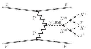
(a) (b)

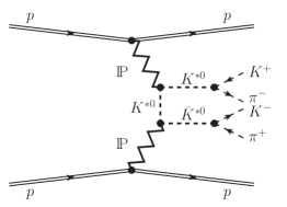
Figure 1: The “Born-level” diagrams for CEP of $K^{*0}\bar{K}^{*0}(\to K^{+}\pi^{-}K^{-}\pi^{+})$ state in proton-proton collisions: (a) the $\mathbb{P}\mathbb{P}\to f_{2}(1950)$ fusion mechanism, (b) the continuum mechanism.

The Born-level amplitude for the $2\to 4$ reaction $p(p_{a},\lambda_{a})+p(p_{b},\lambda_{b})\to p(p_{1},\lambda_{1})+p(p_{2},\lambda_{2})+K^{*0}(p_{3},\lambda_{3})+\bar{K}^{*0}(p_{4},\lambda_{4})$ via the $\mathbb{P}\mathbb{P}\to f_{2}(1950)$ fusion mechanism (Fig. 1 (a)) can be written as

$${\cal M}^{(\mathbb{P}\mathbb{P}\to f_{2}\to K^{*}\bar{K}^{*})}_{\lambda_{a}\lambda_{b}\to\lambda_{1}\lambda_{2}\lambda_{3}\lambda_{4}}=(-i)\,\left(\epsilon^{(K^{*})}_{\kappa_{3}}(\lambda_{3})\right)^{*}\left(\epsilon^{(\bar{K}^{*})}_{\kappa_{4}}(\lambda_{4})\right)^{*}\bar{u}(p_{1},\lambda_{1})i\Gamma^{(\mathbb{P}pp)\,\mu_{1}\nu_{1}}(p_{1},p_{a})u(p_{a},\lambda_{a})$$

$$\qquad\qquad\times i\Delta^{(\mathbb{P})}_{\mu_{1}\nu_{1},\alpha_{1}\beta_{1}}(s_{1},t_{1})i\Gamma^{(\mathbb{P}\mathbb{P}f_{2})\,\alpha_{1}\beta_{1},\alpha_{2}\beta_{2},\rho\sigma}(q_{1},q_{2})\;i\Delta^{(f_{2})}_{\rho\sigma,\alpha\beta}(p_{34})\;i\Gamma^{(f_{2}K^{*}\bar{K}^{*})\,\alpha\beta\kappa_{3}\kappa_{4}}(p_{3},p_{4})$$

$$\qquad\qquad\times i\Delta^{(\mathbb{P})}_{\alpha_{2}\beta_{2},\mu_{2}\nu_{2}}(s_{2},t_{2})\;\bar{u}(p_{2},\lambda_{2})i\Gamma^{(\mathbb{P}pp)\,\mu_{2}\nu_{2}}(p_{2},p_{b})u(p_{b},\lambda_{b})\,,$$ (1)

where $s_{1}=(p_{1}+p_{3}+p_{4})^{2}$, $s_{2}=(p_{2}+p_{3}+p_{4})^{2}$, $q_{1}=p_{a}-p_{1}$, $q_{2}=p_{b}-p_{2}$, $t_{1}=q_{1}^{2}$, $t_{2}=q_{2}^{2}$, and $p_{34}=q_{1}+q_{2}$. The effective pomeron-proton vertex and the tensor-pomeron propagator are [2],

$$i\Gamma_{\mu\nu}^{(\mathbb{P}pp)}(p^{\prime},p)=-i3\beta_{\mathbb{P}NN}F_{1}(t)\left\{\frac{1}{2}\left[\gamma_{\mu}(p^{\prime}+p)_{\nu}+\gamma_{\nu}(p^{\prime}+p)_{\mu}\right]-\frac{1}{4}g_{\mu\nu}(p\!\!\!/^{\prime}+p\!\!\!/)\right\}\,,$$ (2)

$$i\Delta^{(\mathbb{P})}_{\mu\nu,\kappa\lambda}(s,t)=\frac{1}{4s}\left(g_{\mu\kappa}g_{\nu\lambda}+g_{\mu\lambda}g_{\nu\kappa}-\frac{1}{2}g_{\mu\nu}g_{\kappa\lambda}\right)(-is\alpha^{\prime}_{\mathbb{P}})^{\alpha_{\mathbb{P}}(t)-1}\,,$$ (3)

where $\beta_{\mathbb{P}NN}=1.87$ GeV^-1, $F_{1}(t)$ is the Dirac form factor of the proton, and $\alpha_{\mathbb{P}}(t)$ the pomeron trajectory: $\alpha_{\mathbb{P}}(t)=\alpha_{\mathbb{P}}(0)+\alpha^{\prime}_{\mathbb{P}}\,t$, $\alpha_{\mathbb{P}}(0)=1.0808$, $\alpha^{\prime}_{\mathbb{P}}=0.25\;{\rm GeV}^{-2}$ [8]. A possible choice for the $i\Gamma_{\mu\nu,\kappa\lambda,\rho\sigma}^{(\mathbb{P}\mathbb{P}f_{2})(j)}$ coupling terms $j=1,...,7$, derived from a corresponding coupling Lagrangians, is given in [4, 5]. In this work we assume, that only the $j=1$ coupling, corresponding to the lowest values of orbital angular momentum and spin of the two “real pomerons” $(l,S)=(0,2)$, is unequal to zero. The $\mathbb{P}\mathbb{P}f_{2}$ vertex supplemented by form factors is

$$i\Gamma_{\mu\nu,\kappa\lambda,\rho\sigma}^{(\mathbb{P}\mathbb{P}f_{2})}(q_{1},q_{2}) = i\Gamma_{\mu\nu,\kappa\lambda,\rho\sigma}^{(\mathbb{P}\mathbb{P}f_{2})(1)}\tilde{F}_{M}(q_{1}^{2})\tilde{F}_{M}(q_{2}^{2})F^{(\mathbb{P}\mathbb{P}f_{2})}(p_{34}^{2})$$ (4)

$$= i\Gamma_{\mu\nu,\kappa\lambda,\rho\sigma}^{(\mathbb{P}\mathbb{P}f_{2})(1)}\frac{1}{1-t_{1}/\tilde{\Lambda}_{0}^{2}}\;\frac{1}{1-t_{2}/\tilde{\Lambda}_{0}^{2}}\;\frac{\Lambda_{f_{2},P}^{4}}{\Lambda_{f_{2},P}^{4}+(p_{34}^{2}-m_{f_{2}}^{2})^{2}}\,.$$

The $\mathbb{P}\mathbb{P}f_{2}$ coupling constant ($g^{(1)}_{\mathbb{P}\mathbb{P}f_{2}}$) and form-factor cutoff parameters ($\tilde{\Lambda}_{0}$, $\Lambda_{f_{2},P}$) are treated as free parameters which could be adjusted to fit the experimental data. We take a simple Breit-Wigner form for the $f_{2}(1950)$-meson propagator. The $f_{2}K^{*}\bar{K}^{*}$ vertex is as follows ($M_{0}\equiv 1$ GeV):

$$i\Gamma^{(f_{2}K^{*}\bar{K}^{*})}_{\mu\nu\kappa\lambda}(p_{3},p_{4})=i\left[\frac{2g^{\prime}_{f_{2}K^{*}\bar{K}^{*}}}{M_{0}^{3}}\Gamma^{(0)}_{\mu\nu\kappa\lambda}(p_{3},p_{4})F^{\prime}(p_{34}^{2})-\frac{g^{\prime\prime}_{f_{2}K^{*}\bar{K}^{*}}}{M_{0}}\Gamma^{(2)}_{\mu\nu\kappa\lambda}(p_{3},p_{4})F^{\prime\prime}(p_{34}^{2})\right]\,,$$ (5)

with two rank-four tensor functions (see Eqs. (3.18) and (3.19) of [3]). Here we assume $F^{\prime(f_{2}K^{*}\bar{K}^{*})}=F^{\prime\prime(f_{2}K^{*}\bar{K}^{*})}=F^{(\mathbb{P}\mathbb{P}f_{2})}$ and $\Lambda^{\prime}_{f_{2}}=\Lambda^{\prime\prime}_{f_{2}}=\Lambda_{f_{2},P}$. Thus, the result depends on $\Lambda_{f_{2},P}$ and the product of the couplings $g^{(1)}_{\mathbb{P}\mathbb{P}f_{2}}g^{\prime}_{f_{2}K^{*}\bar{K}^{*}}$ or $g^{(1)}_{\mathbb{P}\mathbb{P}f_{2}}g^{\prime\prime}_{f_{2}K^{*}\bar{K}^{*}}$. In the following we assume that only either the first or the second of the product of couplings is nonzero.

In the continuum mechanism, we take into account the reggeization of intermediate $K^{*}$ meson; see [2]. We used two parametrisations of the $K^{*}$ trajectory: linear and nonlinear (square-root form) [10]. The $\mathbb{P}K^{*}K^{*}$ vertex, with $k^{\prime},\mu$ and $k,\nu$ the momentum and vector index of the outgoing and incoming $K^{*}$, respectively, and $\kappa\lambda$ the tensor $\mathbb{P}$ indices, reads

$$i\Gamma^{(\mathbb{P}K^{*}K^{*})}_{\mu\nu\kappa\lambda}(k^{\prime},k)=i\left[2a_{\mathbb{P}K^{*}K^{*}}\Gamma^{(0)}_{\mu\nu\kappa\lambda}(k^{\prime},-k)-b_{\mathbb{P}K^{*}K^{*}}\,\Gamma^{(2)}_{\mu\nu\kappa\lambda}(k^{\prime},-k)\right]\frac{1}{1-(k^{\prime}-k)^{2}/\Lambda_{0}^{2}}\hat{F}_{K^{*}}(\hat{p}^{2}).$$ (6)

Here, the form factors $\hat{F}_{K^{*}}(\hat{p}_{t}^{2})$ and $\hat{F}_{K^{*}}(\hat{p}_{u}^{2})$ are parametrised in the exponential form. We assume that $a\neq 0$, $b=0$ or $a=0$, $b\neq 0$. The coupling and cutoff parameters ($a_{\mathbb{P}K^{*}K^{*}}$, $b_{\mathbb{P}K^{*}K^{*}}$, $\Lambda_{0}$, $\Lambda_{\rm off,E}$) could be adjusted to experimental data; see Ref. [2] for their numerical values and for more details.

2 Comparison with the WA102 data and predictions for the LHC experiments

In our exploratory study we consider separately the two mechanisms shown by the diagrams in Fig. 1. We obtain a good description of the WA102 data [9] for the reaction $pp\to ppK^{*0}\bar{K}^{*0}$ assuming the dominance of pomeron-pomeron fusion already at $\sqrt{s}=29.1~{}{\rm GeV}$ (Fig. 2). The model results, in both cases, are in better agreement with the WA102 data for the tensor-vector-vector coupling vertices $\propto\Gamma^{(2)}$. The absorption effects were included. Absorption effects lead to a reduction of the cross section and change the shape of the $\phi_{pp}$ distribution, the azimuthal angle between the transverse momentum vectors of the outgoing protons. Both considered mechanisms have a maximum around $M_{2K2\pi}\simeq 2$ GeV (see Fig. 3), thus a broad enhancement in this mass region can be misidentified as the $f_{2}(1950)$ resonance (one of the tensor glueball candidates). The predictions for the LHC experiments should be regarded rather as an upper limit.

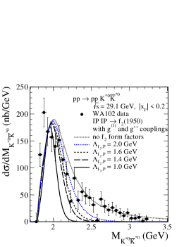
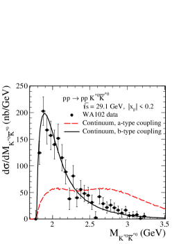
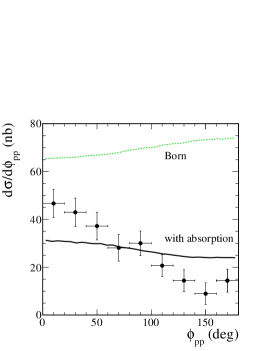
Figure 2: The distributions in $K^{*0}\bar{K}^{*0}$ invariant mass for the $f_{2}(1950)$ mechanism (left), for the continuum mechanism (center), and the $\phi_{pp}$ distribution (right) together with the WA102 data ($\sigma_{\rm exp}=85\pm 10~{}{\rm nb}$ [9]).

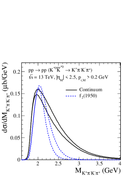
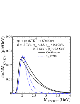
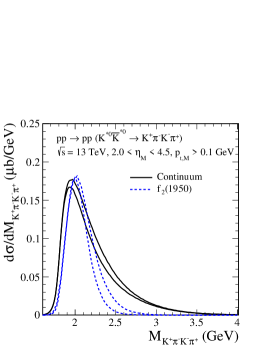
Figure 3: Invariant mass distributions for the $K^{+}\pi^{-}K^{-}\pi^{+}$ system calculated for $\sqrt{s}=13~{}{\rm TeV}$. We show the results with cuts on pseudorapidities and transverse momenta of produced pions and kaons, and with an extra cuts on momenta of outgoing protons that will be measured in the ATLAS+ALFA experiment (in the middle panel), and the results for larger $\eta_{M}$ and without a measurement of protons relevant for the LHCb experiment (right panel). For the continuum term we show the results for two parametrisations of the $K^{*}$ trajectory: the linear form (lower solid line) and the nonlinear form (upper solid line). For the $f_{2}$ contribution the results for $\Lambda_{f_{2},P}$ = 1.6 GeV (lower dotted line), 2 GeV (upper dotted line), and with $|g^{(1)}_{\mathbb{P}\mathbb{P}f_{2}}g^{\prime\prime}_{f_{2}K^{*}\bar{K}^{*}}|=11$ are presented.

3 Conclusions

• The calculation for the $pp\to ppK^{*0}\bar{K}^{*0}$ reaction have been performed in the tensor-pomeron approach [3]. We have discussed CEP of the $f_{2}(1950)$ resonance and the continuum with the intermediate $K^{*}$-reggeized exchange. We obtain a good description of the WA102 data with the continuum contribution alone, assuming that the reaction is dominated by pomeron-pomeron fusion.

• Predictions for the reaction $pp\to ppK^{+}K^{-}\pi^{+}\pi^{-}$ for the LHC experiments at $\sqrt{s}=13~{}{\rm TeV}$ were given. We obtain $\sigma\simeq 17-250~{}{\rm nb}$ depending on the assumed cuts. Absorption effects were included. Similar behaviour of considered mechanisms (Fig. 1) makes an identification of a broad tensor-glueball state in this reaction rather difficult.

References

- [1]
- [2] P. Lebiedowicz, Phys. Rev. D 103 (2021) 054039.
- [3] C. Ewerz, M. Maniatis, and O. Nachtmann, Annals Phys. 342 (2014) 31.
- [4] P. Lebiedowicz, O. Nachtmann, and A. Szczurek, Phys. Rev. D 93 (2016) 054015.
- [5] P. Lebiedowicz, O. Nachtmann, and A. Szczurek, Phys. Rev. D 101 (2020) 034008.
- [6] P. Lebiedowicz, O. Nachtmann, and A. Szczurek, Annals Phys. 344 (2014) 301.
- [7] P. Lebiedowicz et al., Phys. Rev. D 102 (2020) 114003.
- [8] A. Donnachie, H. G. Dosch, P. V. Landshoff, and O. Nachtmann, Pomeron physics and QCD, Camb. Monogr. Part. Phys. Nucl. Phys. Cosmol. 19 (2002) 1–347.
- [9] D. Barberis et al., (WA102 Collaboration), Phys. Lett. B436 (1998) 204.
- [10] M. M. Brisudová, L. Burakovsky, and T. Goldman, Phys. Rev. D 61 (2000) 054013.