Driving determines the dynamics in transitional pipe flows

Abstract

The transition to turbulence in a long, straight pipe is one of the outstanding unresolved problems in classical Physics. It is well-established by experiments that a finite amplitude disturbance is required to trigger the transition to turbulence from laminar flow. Details of the processes involved in the transition are mysterious and a full understanding of them remains aloof. Here we take the novel approach of initiating the flow in a turbulent state and then reducing the flow rate suddenly, a so-called quench, so that the flow decays from turbulence. We use two distinct methods of driving the flow and find that the dynamical processes involved in the decay, as well as the fraction of the flow that remains turbulent, are qualitatively distinct for each driving protocol.

1 Introduction

Despite over a hundred years of intense study, it is a significant challenge to give a precise prediction for when and how the flow in a straight pipe will become turbulent Mullin (2011); Eckhardt et al. (2007). One reason for this is that many features of the transition between quiescent laminar flow and chaotic turbulent flow depend sensitively on the spatio-temporal details of the triggering perturbation, such as its amplitude or geometry Hof et al. (2003); Tasaka et al. (2010); Peixinho & Mullin (2007); Mellibovsky & Meseguer (2006). The focus of much work has been to characterize robust features such as the existence of localized patches of turbulence broadly categorized into regularly-sized “puffs” and ever-growing “slugs” over a range of Reynolds numbers. These discrete patches themselves possess reproducible features such as puff decay Peixinho & Mullin (2006); Kuik et al. (2010), both puff decay and splitting Nishi et al. (2008); Avila et al. (2011), and slug growth rates Wygnanski & Champagne (1973); Nishi et al. (2008); Barkley et al. (2015). So long as the finite-amplitude perturbation’s amplitude was large enough to trigger the puff or slug at the given Reynolds number Hof et al. (2003), these reproducible features are assumed to be independent of their origin sufficiently far downstream Mullin (2011); Eckhardt et al. (2007). While the prevailing assumption has been that these features will then depend only on the Reynolds number, here we show through extensive experiments that the method of driving must also be taken into account when characterising the transition.

The focus of our study is the influence of the method used to drive the flow on the observed dynamical motion in the transition regime. The most common method to drive the flow is to use a controlled pressure gradient. This is typically achieved in transition experiments using liquids with a supply tank and an overflow to apply a constant pressure gradient (CPG) along the pipe which in turn sets the Reynolds number, $Re=UD/\nu$, where $U$ is the flow speed, $D$ is the pipe diameter, and $\nu$ is the kinematic viscosity, the standard control parameter of pipe flow Tietjens & Prandtl (1957); Tritton (2012); Rotta (1956). On transition there is an increase in friction factor or resistance to flow which gives rise to fluctuations in $Re$ Cerbus (2022). A successful strategy for minimising these fluctuations is to introduce a large external resistance in series with the pipe Rotta (1956); Avila et al. (2011) so that the pressure drop along the pipe is much smaller than that across the entire system. This approach can be used to reduce fluctuations to $\lessapprox 1\%$ in CPG driven flows Barkley et al. (2015).

The alternative approach is to use a mass displacement device such as a piston driven at constant speed to move the flow Darbyshire & Mullin (1995); Peixinho & Mullin (2006). This method controls the $Re$ directly by driving the flow at constant mass flux (CMF). Clearly, this method can only operate for a finite period of time but when suitably designed this is not a severe limitation in practice. It is known that fluctuations in $Re$ are small for both CPG with a large external resistance and CMF flows and hence it might be anticipated that closely similar results will be obtained. However, experiments using the two different driving mechanisms outlined above have produced observations of different $Re$-dependence for the decay lifetimes of puffs Avila et al. (2011); Kuik et al. (2010); Peixinho & Mullin (2006), and no puff splitting has been reported in experimental CMF flows Darbyshire & Mullin (1995). Just as differences between CMF and CPG flow have been noted in a study of subcritical instability of channel flow Rozhdestvensky & Simakin (1984), these two sets of experiments suggest that the different driving mechanisms may produce qualitatively distinct outcomes. However, it has also been argued that this discrepancy results from differences in pipe lengths Mukund & Hof (2018) or initial conditions Avila et al. (2010). The qualitative difference in the decay of puffs under CPG and CMF conditions for moderate length pipes Kuik et al. (2010) are also found in the much longer pipes used in the current investigation, in which we have also performed experiments at several pipe lengths to account for any potential influence of length as discussed below. A main objective of our investigation is to both minimise differences in initial conditions as practicably as possible and account for differences in pipe length so as to demonstrate that in the transitional regime, CPG and CMF flows behave differently, and that the driving determines both the dynamics and the long-term behavior.

It is well accepted that Poiseuille pipe flow is linearly stable Kerswell (2005) and a finite amplitude disturbance is required to cause a transition to turbulence Mullin (2011). In practice the amplitude of the disturbance required for transition is large in the range of $Re$ studied here and obtaining systematic behaviour using a direct approach of introducing a disturbance over the required range of $Re$ is fraught with difficulties Darbyshire & Mullin (1995). Hence we circumvented these complications by starting from a well-defined state: turbulence at a value $Re$ above the transition regime. We then perform a quench, quickly reducing $Re$ to a target value in the transition regime, and observe the ensuing decay. Relying on the universality of turbulence to study its decay is a well-established technique. Batchelor and Townsend, for example, performed decay experiments starting from the turbulent state to establish that viscous dissipation sets the time scale of the final decay Batchelor & Townsend (1948). Likewise this approach is similar to previous CMF pipe experiments studying individual puffs Peixinho & Mullin (2006), transitional plane Couette flow experiments Bottin et al. (1998), and plane Couette-Poiseuille flow experiments Liu et al. (2021), but now we use it for both CMF and CPG pipe flows. There is numerical evidence Quadrio et al. (2016) that the initial conditions will be essentially the same for the turbulent state in both flows, but we find that the resulting flow behavior, in particular the behaviour of the fraction of the flow that is turbulent, $\gamma(t)$, is decidedly different in the transition regime.

2 The Experiments and Protocol

Figure 1: Pipe experiment schematics modelled after that appearing in Reynolds (1883). Flow is from left to right. Straight horizontal lines indicate laminar flow, and jagged lines indicate turbulence. (a) The constant pressure gradient (CPG) pipe experiments have a reservoir placed above the pipe to drive the flow. (b) The CMF pipe experiments use two motor-driven syringes to drive the flow. All experimental setups use a contracting entrance section and a series of meshes and grids to establish laminar flow at the entrance. An obstacle is used to perturb the flow. The pressure drop $\Delta P$ is measured over a distance $\Delta L$ near the end of the pipes which have a total length of $L_{\rm{tot}}$. The effective length of the pipe useful for the present study is a distance $L$ which is the distance from the beginning of the disturbance to the end of the pressure measurement section.

The main diagnostic tool we use to probe the dynamical state of the flow is the turbulent fraction $\gamma(t)$. This has become a common diagnostic for transitional flows, where the regions of turbulent flow are identified by, for example, setting a threshold on the local velocity fluctuations and setting $\gamma(t)$ as the ratio of the size of these regions to the total size of the probed region Rotta (1956); Mukund & Hof (2018); Moxey & Barkley (2010); Bottin et al. (1998). Here we use a new procedure that avoids the ambiguity of a threshold by determining $\gamma(t)$ through the friction factor $f(t)=(2D\Delta P(t)/\Delta L)/(\rho U(t)^{2})$, where $\Delta P(t)$ is the pressure drop over a distance $\Delta L$, $D$ is the pipe diameter, $\rho$ is the density, and $U(t)$ is the instantaneous flow speed. We exploit the fact that the friction factor $f(t)$ follows the Blasius (turbulent) friction law even in the transient puffs and slugs Cerbus et al. (2018). When a flow is fully laminar over $\Delta L$, then $f(t)=f_{\rm{lam}}=64/Re(t)$, the Hagen-Poiseuille friction law. If the flow is fully turbulent, then $f(t)=f_{\rm{turb}}=0.3164Re(t)^{-1/4}$, the Blasius (turbulent) friction law. If the flow is intermittent, the friction factor is given by a weighted average between the two laws Cerbus et al. (2018): $f(t)=\gamma(t)f_{\rm{turb}}+(1-\gamma(t))f_{\rm{lam}}$, where $\gamma(t)$ is the weight. This can be rearranged to find the instantaneous $\gamma(t)$ by measuring $f(t)$: $\gamma(t)=(f(t)-f_{\rm{lam}})/(f_{\rm{turb}}-f_{\rm{lam}})$. Although this method of determining $\gamma(t)$ avoids the inherent ambiguity of setting a threshold on quantities such as the turbulence intensity Moxey & Barkley (2010), it also allows for values of $\gamma(t)>1$ if $f(t)>f_{\rm{turb}}$, which can occur in the early stages of the quench before the flow equilibrates. (While $f_{\rm{lam}}$ is a strict lower bound for $f(t)$, $f_{\rm{turb}}$ is not a strict upper bound Plasting & Kerswell (2005).) We discuss below how $f(t)$ is determined in both the CPG and CMF pipe experiments.

Our experiments were performed using three separate pipes, the flows in two of which are driven by gravity (CPG), and one is driven by high-pressure syringe pumps (CMF) as shown in schematic form in Fig. 1a,b . The two CPG flows are similar to other CPG transition pipe experiments Mullin (2011); Barkley et al. (2015). They are each 20-m-long, made of 1-m-long accurate bore cylindrical glass tubes with diameter $D$ = 2.5 cm $\pm$ 10 $\mu$m ($L_{\rm{tot}}/D=808$), and $D$ = 1 cm $\pm$ 10 $\mu$m ($L_{\rm{tot}}/D=2020$), joined by acrylic connectors. Some of the connectors contain pairs of diametrically-opposite holes ($\sim$ 1 mm diameter) which are used as pressure taps. The total pressure gradient was set by the height difference between the reservoir and the pipe outlet. This could be adjusted by changing the height of the reservoir and further control over the flow rate was provided by a ball valve located adjacent to the reservoir. The CPG flow can remain laminar at the highest $Re$ tested, $Re\approx 10,000$, and in addition to the ball valve we use an external resistance to damp fluctuations in $Re$ so that it remains constant even in the transition regime to within $\lesssim$ 1% and $\lesssim$ 2% for the $D$ = 2.5 cm and 1 cm pipes, respectively.

The CMF experimental setup (Fig. 1b) is driven by two independent, computer-controlled, high-pressure syringe pumps (Chemyx Fusion 6000). The pipe is 14-m-long, made of 1-m-long cylindrical glass tubes (Duran) of inner diameter $D$ = 0.3 cm $\pm$ 10 $\mu$m ($L_{\rm{tot}}/D=4840$), joined by 3D-printed and machined plastic connectors. All the connectors have diametrically-opposite holes (of diameter $\sim$ 1 mm) to enable the measurement of the pressure drop $\Delta P(t)$ along the pipe. In the present investigation we focus on measurements near the end of the pipe. We determined an in situ pressure sensor calibration for all flows using laminar flow as a reference. For the CMF setup the flow speed $U(t)$ is controlled while for the CPG setups it is measured with a Yokogawa magnetic flowmeter. We confirmed the accuracy of both by weighing the amount of water exiting the pipe and in a set time period which was measured using a stopwatch. The Yokogawa floweter agreed to within $\lesssim 1\%$ and the syringe pumps to within $\lesssim 0.1\%$. In all experiments the flow was conditioned before entering the test section. The CMF flow can remain laminar till the highest $Re$ achievable with a single pump, $Re\approx 3,100$.

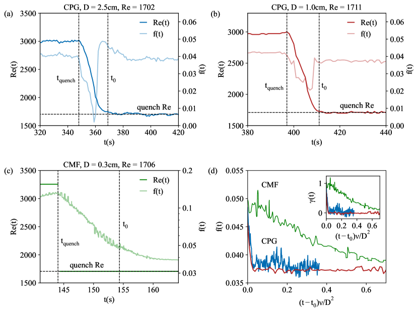
Figure 2: Example time series of $Re(t)$ and $f(t)$ for quenching experiments using (a) a $D=2.5$cm pipe flow under CPG driving, (b) a $D=1.0$cm pipe with CPG driving and (c) a $D=0.3$cm pipe with CMF driving. The final quench value is $Re\simeq 1700$ in all cases. In the case of the CPG experiments the $t_{0}$ point is identified as the time when $Re(t)$ lies within the fluctuations about the averaged final quenched value, while for the CMF flow it is identified as the first time when the $\gamma(t)\simeq 1$ within the fluctuations. (d) All three example time series rescaled by the viscous diffusion time $D^{2}/\nu$ illustrating that the disparate timescales of the flows in the range of pipe diameters scale appropriately. Inset: the same data as in (d) but now converted to the turbulent fraction $\gamma(t)$.

We use Labview and a DAQ board with all setups to determine $Re(t)$, $f(t)$, and thus $\gamma(t)$, simultaneously. Due to the different time scales of the experiments and limitations of the sensors, the sampling rate for the CPG pipe flows was typically 1Hz while for the CMF flow it was 100Hz or faster. The pressure measurement section of length $\Delta L$ is downstream of the entrance.

The temperature remained constant to within $\lesssim$ 0.03 K during an experiment, which yields variations in $Re$ of $\delta Re\lesssim 2$. Using two CPG pipes of different diameter allows us to test both the role of (effective) pipe length, $L/D$, and quench duration $\Delta TU/D$, in otherwise identical experimental conditions. The time to perform the quench for the CPG experiments was fixed by the time required to lower the reservoir which was $\Delta T\sim 11$s while for CMF this was set by the stopping time for the piston which was $\Delta T\sim 0.4$s. For the $D=2.5$, $D=1$ and $D=0.3$ cm pipes, $\Delta TU/D\simeq 33$, $\Delta TU/D\simeq 205$, and $\Delta TU/D\simeq 82$, respectively, at $Re=2000$.

In order to establish a turbulent initial state, we trigger the flow upstream using an asymmetric, Teflon obstacle of a selected size. We take advantage of the finite amplitude instability of pipe flow Mullin (2011) to adjust the obstacle such that it triggers turbulence only when $Re\gtrsim 3000$, outside of the transition regime. In this way we can raise the $Re$ of the flow above $Re\simeq 3000$ to establish a turbulent state. We determined in a series of experiments that details of the quench protocol, such as the initial $Re$ or quench time, are not important. When we reduce the $Re$ to a target value inside the transitional regime ($1500\lesssim Re\lesssim 2700$), the obstacle does not trigger turbulence. We do not consider the flow beyond $t>(L-\Delta L)/U$, the time it takes the fluid from the entrance to reach the pressure measurement section a distance $L-\Delta L$ downstream (see Fig. 1). We also set a starting point of the quench time series $t=t_{0}$ according to an empirically-determined settling time after quenching, similar to the formation time used in puff lifetime studies Kuik et al. (2010); Avila et al. (2011). For the CPG experiments this was the time for $Re(t)$ to reach the target quench $Re$ value within fluctuations (often $t_{0}-t_{\rm{quench}}\sim 20$s). For the CMF flow we chose to instead determine $t_{0}$ as the time when the turbulent fraction $\gamma(t)$ reached unity within fluctuations (often $t_{0}-t_{\rm{quench}}\sim 10$s), in order to better compare the subsequent behavior of CPG and CMF (see Darbyshire & Mullin (1995); Das & Arakeri (1998)). However, we confirmed that changing the value of $t_{0}$ by a factor of two changes our estimates of the decay time by $\lesssim 10\%$, which is negligible compared to the difference between CMF and CPG (Fig. 4a) and has no effect on the estimate of the long-time behavior (Fig. 4b).

The experimental protocols used for both CPG and CMF flows are illustrated by the example sets of time-series given in Figs. 2a,b,c. For $t<0$, the flow is initiated at $Re\gtrsim 3000$ and the obstacle placed in the flow induces a disordered flow. In principle, the disorder could contain structures but the repeatability of our results suggest that, if present, they do not play a significant role in the subsequent decay dynamics. Next, after the disorder has spread throughout the length of the pipe, the flow is quenched by suddenly reducing $Re$. For the CPG experiments the quench is accomplished by lowering the reservoir, while for the CMF flow it is achieved by stopping one of the two high-pressure syringe pumps. We use the value of $f(t)$ in the range $t_{0}\leq t\leq(L-\Delta L)/U$ to determine $\gamma(t)$. We perform each experiment between three and ten times and then ensemble-average the $\gamma(t)$ curves from each run. We performed $\sim$ 400 rehearsals of the experiments over a period of $\sim$ 40 months in an air-conditioned laboratory environment, with the experimental run time collectively reaching $\sim$ 3.5$\times 10^{5}$ advective time units.

The time sequences for the CPG experiments are qualitatively indistinguishable as can be seen in Fig. 2a,b,d. However, the mean flow speeds are significantly higher in the CMF experiments and the overall physical timescales are much shorter as can be seen in Fig. 2c. Nevertheless, satisfactory scaling of time can be achieved using viscous diffusion $\frac{D^{2}}{\nu}$ as shown in Fig. 2d.

3 Results

3.1 Time series of $\gamma(t)$

Figure 3: Illustrative plots of turbulent fraction $\gamma(t)$ vs. scaled time $tU/L$ for both CMF and CPG experiments with $t_{0}-t_{\rm{quench}}\sim 10$s for CMF flow and $\sim$ 20s for CPG flows. (a) The final value of $Re$ lies in the range $\sim 1700$ to $\sim 1950$ and $\gamma(t)$ decays exponentially ($--$), with a decay exponent $\tau$ that increases with $Re$ (see Fig. 4a). A clear difference can be seen between the CMF and CPG results as the CMF time series indicate a decay to a finite plateau value ($\cdot\cdot\cdot$) of $\gamma(t)$ whereas the CPG results decay to zero much faster at the same values of $Re$. (b) Time series for both CPG and CMF for $Re$ above $Re\sim 2000$. Now after the initial decay a plateau ($\cdot\cdot\cdot$) develops also for the CPG flows. The CMF time series have consistently higher values of $\gamma(t)$ than the CPG results for the same $Re$.

As a first step in understanding the differences between CMF and CPG driven pipe flows, we plot in Fig. 3a several time series of the turbulent fraction $\gamma(t)$ versus normalized time $tU/L$, where $U$ is the flow speed at the target $Re$. As can be seen in Fig. 3a for both CMF and CPG ($D=2.5$ cm) flows, the initially turbulent state decays approximately exponentially ($--$) for a range of $Re$. Given that the observations of the probability of decay of individual puffs decays exponentially in time for both CMF Peixinho & Mullin (2006) and CPG flows Avila et al. (2011); Kuik et al. (2010), it is perhaps not surprising that $\gamma(t)$, representing the combined contribution of all present puffs and laminar flow, should also decay exponentially. However, it is clear that there are systematic and qualitatively distinct differences between the two sets of decays here and compared to previous work on puff decay. For $Re\lesssim 2000$ the CPG driving invariably leads to decay to Poiseuille flow whereas CMF driving gives rise to sustained disorder of the flow beyond $Re\gtrapprox 1750$ which systematically increases as the final value of $Re$ is increased. For $Re\gtrapprox 2000$ (see Fig.3b), after the initial decay, a non-zero plateau is rapidly established also for the CPG flow, taking more time for the CMF flow.

The decay rates observed here (see Fig. 4a) differ significantly from individual puff decay rates measured previously Peixinho & Mullin (2006); Avila et al. (2010). The flow behavior is clearly more than simply the sum of the decay of its individual puffs. In addition to puff decay Peixinho & Mullin (2006); Avila et al. (2011); Kuik et al. (2010), it is likely that puff splitting Nishi et al. (2008), puff interactions Samanta et al. (2011), and the progression from puffs to slugs Mullin (2011) combine in a non-trivial way to produce the rich behavior observed here. Thus the curves in Fig. 3 represent global temporal behavior, whereas measurements of individual puffs reveal local behavior Moxey & Barkley (2010).

Figure 4: (a) Log-log plot of the normalized decay times $\tau U/D$ vs. $Re$ for CMF and CPG flows. $\tau U/D$ appears to grow as a power-law with $Re$ for the CMF flows ($--$), while for the CPG flows the slight increase in slope with $Re$ suggests an exponential fit ($\cdot\cdot\cdot$). The $L/D=4162$ CMF measurements were made upstream of the $L/D=4502$ measurements to investigate the effect of pipe length for CMF flow, which is imperceptible for the decay times and tends to increase $\langle\gamma\rangle$ by $\sim 5\%$ on average. The CMF decay times are larger than their CPG counterparts by an order of magnitude. (b) Plot of the plateau value $\langle\gamma\rangle$ vs. $Re$. Vertical error bars are the standard deviation of the mean, and horizontal error bars are the standard deviation of the instantaneous fluctuations in $Re$ after the quench. A comparison with results from the literature Mukund & Hof (2018) indicates that the CPG results are insensitive to either pipe length or initial conditions. The respective deviations from $\langle\gamma\rangle=0$ occur at $Re$ close to critical values previously found in studies of single puff decay ($Re_{c}^{\rm{CMF}}\simeq 1750$, $--$; $Re_{c}^{\rm{CPG}}\simeq 2040$, $\cdot\cdot\cdot$) Peixinho & Mullin (2006); Avila et al. (2011). The most striking conclusion from both comparisons is that both the dynamic and stationary behavior of CMF flow is qualitatively different from CPG flow.

3.2 $Re$-dependence of the decay and plateau

In order to understand the behavior of quenched flow, and thus the differences between CMF and CPG flow, we must characterize both the initial decay and the final plateau. This leads us to our main and most striking results. First, we investigate the exponential decay times $\tau U/D$ vs. $Re$ in Fig. 4a, where $\tau$ is determined by an exponential fit to $\gamma(t)$ until it decays by half. As Fig. 3 already indicates, the quench decay times for CMF flow are significantly longer than for CPG flow, just as single puffs survive longer in CMF flow than in CPG flow at the same $Re$ Peixinho & Mullin (2006); Avila et al. (2011); Kuik et al. (2010). We note that the longer lifetimes of CMF flow may offer a unique opportunity to study the decay of turbulence at very low $Re$ and seek for special solutions to the Navier-Stokes equations such as the periodic states found in plane Poiseuille flow Reynolds & Potter (1967); Pekeris & Shkoller (1967); Herbert (1979).

Next we examine the average turbulent fraction $\langle\gamma\rangle$ vs. $Re$ in Fig. 4b, where we have averaged over the end (typically $1/5$) of the ensemble-averaged times series $\gamma(t)$ as an estimate of the plateau values $\gamma(Re,t\rightarrow\infty)$. Just as with the dynamics, the stationary behavior of the quenched CMF and CPG flows differs considerably. The CMF $\langle\gamma\rangle$ curve peels away from zero at a critical $Re_{C}\simeq 1750$ and continues to rise while the CPG curve remains at zero until $Re_{C}\simeq 2000$, thus yielding $Re_{C}$ that are close to previous literature values Peixinho & Mullin (2006); Avila et al. (2011). These differences are outside the statistical uncertainty and cannot be explained by differences in $L/D$ as the CPG span over an order of magnitude in $L/D$ and yet coincide, and artificially decreasing $L/D$ for the CMF flow by measuring the pressure further upstream also makes little difference for either $\tau U/D$ or $\langle\gamma\rangle$. Although we took great care to use initial conditions which were practically the same, a comparison with other CPG experiments with a larger $L/D$ and starting from substantially different initial conditions, individual puffs, are in accord with the same $\langle\gamma\rangle$ curve Mukund & Hof (2018), underscoring its robustness. The only relevant difference appears to be the driving mechanism.

The coincidence between the $Re_{C}$ observed here and the values determined by examining individual puffs suggests that the dynamics of single puffs controls the critical $Re_{C}$ Mukund & Hof (2018). As $Re$ increases beyond $Re_{C}$, however, it is likely that additional physics such as puff interactions influence the flow behavior. Similarly it is likely that the same interactions are the cause of the small quench decay rate relative to the single puff decay rate in CPG Avila et al. (2011); Kuik et al. (2010).

4 Conclusions

The principle conclusion of this experimental study is that CMF and CPG flows are not the same, despite the flows being dynamically similar on average, in the same range of $Re$, and with statistically similar initial conditions. The method of driving must be taken into account when investigating the dynamics of the flow. We suggest that the origin of the difference between CMF and CPG flow might be understood by a detailed investigation of the differences between puffs in these two apparently distinct flows, where the decay statistics differ and where in CMF flows puff splitting has not been observed Darbyshire & Mullin (1995). Likewise the correspondence between the putative maximum $\langle\gamma\rangle$ set by puff interactions and the quenched $\langle\gamma\rangle$ (for CPG) indicates that a better understanding of interactions is also needed. In conclusion, our extensive experimental work highlights the complexity of transitional pipe flow and identifies the need for further investigation, but also points to the important role of puff interactions and the possibility to use CMF flow for investigations of stable states at low $Re$ not previously accessible.

[Acknowledgements]We thank Jorge Peixinho, Pinaki Chakraborty, and Hamid Kellay for helpful comments.

[Funding]R.T.C. gratefully acknowledges funding from the Horizon 2020 program under the Marie Skłodowska-Curie Action Individual Fellowship (MSCAIF) No. 793507, the support of JSPS (KAKENHI Grant No. 17K14594), and the support of the Okinawa Institute of Science and Technology (OIST) where the experiments were carried out.

[Declaration of interests]The authors report no conflict of interest.

[Data availability statement]The data that support the findings of this study are available upon reasonable request to the authors.

[Author ORCIDs]R.T. Cerbus, https://orcid.org/https://orcid.org/0000-0002-2162-1039

References

- Avila et al. (2011) Avila, Kerstin, Moxey, David, de Lozar, Alberto, Avila, Marc, Barkley, Dwight & Hof, Björn 2011 The onset of turbulence in pipe flow. Science 333 (6039), 192–196.
- Avila et al. (2010) Avila, Marc, Willis, Ashley P & Hof, Björn 2010 On the transient nature of localized pipe flow turbulence. Journal of fluid mechanics 646, 127–136.
- Barkley et al. (2015) Barkley, Dwight, Song, Baofang, Mukund, Vasudevan, Lemoult, Grégoire, Avila, Marc & Hof, Björn 2015 The rise of fully turbulent flow. Nature 526 (7574), 550–553.
- Batchelor & Townsend (1948) Batchelor, George Keith & Townsend, Albert Alan 1948 Decay of turbulence in the final period. Proceedings of the Royal Society of London. Series A. Mathematical and Physical Sciences 194 (1039), 527–543.
- Bottin et al. (1998) Bottin, Sabine, Daviaud, Francois, Manneville, Paul & Dauchot, Olivier 1998 Discontinuous transition to spatiotemporal intermittency in plane couette flow. EPL (Europhysics Letters) 43 (2), 171.
- Cerbus (2022) Cerbus, Rory T 2022 Prandtl-tietjens intermittency in transitional pipe flows. Physical Review Fluids 7 (1), L011901.
- Cerbus et al. (2018) Cerbus, Rory T, Liu, Chien-Chia, Gioia, Gustavo & Chakraborty, Pinaki 2018 Laws of resistance in transitional pipe flows. Physical Review Letters 120 (5), 054502.
- Darbyshire & Mullin (1995) Darbyshire, AG & Mullin, T 1995 Transition to turbulence in constant-mass-flux pipe flow. Journal of Fluid Mechanics 289, 83–114.
- Das & Arakeri (1998) Das, Debopam & Arakeri, Jaywant H 1998 Transition of unsteady velocity profiles with reverse flow. Journal of Fluid Mechanics 374, 251–283.
- Eckhardt et al. (2007) Eckhardt, Bruno, Schneider, Tobias M, Hof, Bjorn & Westerweel, Jerry 2007 Turbulence transition in pipe flow. Annu. Rev. Fluid Mech. 39, 447–468.
- Herbert (1979) Herbert, Thorwald 1979 Periodic secondary motions in a plane channel. In Proceedings of the Fifth International Conference on Numerical Methods in Fluid Dynamics June 28–July 2, 1976 Twente University, Enschede, pp. 235–240. Springer.
- Hof et al. (2003) Hof, Björn, Juel, Anne & Mullin, T 2003 Scaling of the turbulence transition threshold in a pipe. Physical review letters 91 (24), 244502.
- Kerswell (2005) Kerswell, R R. 2005 Recent progress in understanding the transition to turbulence in a pipe. Nonlinearity 18, R17.
- Kuik et al. (2010) Kuik, Dirk Jan, Poelma, C & Westerweel, Jerry 2010 Quantitative measurement of the lifetime of localized turbulence in pipe flow. Journal of fluid mechanics 645, 529–539.
- Liu et al. (2021) Liu, T, Semin, B, Klotz, Lukasz, Godoy-Diana, R, Wesfreid, JE & Mullin, T 2021 Decay of streaks and rolls in plane couette–poiseuille flow. Journal of Fluid Mechanics 915.
- Mellibovsky & Meseguer (2006) Mellibovsky, Fernando & Meseguer, Alvaro 2006 The role of streamwise perturbations in pipe flow transition. Physics of Fluids 18 (7), 074104.
- Moxey & Barkley (2010) Moxey, David & Barkley, Dwight 2010 Distinct large-scale turbulent-laminar states in transitional pipe flow. Proceedings of the National Academy of Sciences 107 (18), 8091–8096.
- Mukund & Hof (2018) Mukund, Vasudevan & Hof, Björn 2018 The critical point of the transition to turbulence in pipe flow. Journal of Fluid Mechanics 839, 76–94.
- Mullin (2011) Mullin, T 2011 Experimental studies of transition to turbulence in a pipe. Annual Review of Fluid Mechanics 43, 1–24.
- Nishi et al. (2008) Nishi, Mina, Ünsal, Bülent, Durst, Franz & Biswas, Gautam 2008 Laminar-to-turbulent transition of pipe flows through puffs and slugs. Journal of Fluid Mechanics 614, 425–446.
- Peixinho & Mullin (2006) Peixinho, Jorge & Mullin, Tom 2006 Decay of turbulence in pipe flow. Physical review letters 96 (9), 094501.
- Peixinho & Mullin (2007) Peixinho, Jorge & Mullin, Tom 2007 Finite-amplitude thresholds for transition in pipe flow. Journal of Fluid Mechanics 582, 169–178.
- Pekeris & Shkoller (1967) Pekeris, Chaim L & Shkoller, Boris 1967 Stability of plane poiseuille flow to periodic disturbances of finite amplitude in the vicinity of the neutral curve. Journal of Fluid Mechanics 29 (1), 31–38.
- Plasting & Kerswell (2005) Plasting, SC & Kerswell, RR 2005 A friction factor bound for transitional pipe flow. Physics of Fluids 17 (1), 011706.
- Quadrio et al. (2016) Quadrio, Maurizio, Frohnapfel, Bettina & Hasegawa, Yosuke 2016 Does the choice of the forcing term affect flow statistics in dns of turbulent channel flow? European Journal of Mechanics-B/Fluids 55, 286–293.
- Reynolds (1883) Reynolds, Osborne 1883 An experimental investigation of the circumstances which determine whether the motion of water shall be direct or sinuous, and of the law of resistance in parallel channels. Proceeds of the Royal Society of London 35, 84–99.
- Reynolds & Potter (1967) Reynolds, WC & Potter, Merle C 1967 Finite-amplitude instability of parallel shear flows. Journal of Fluid Mechanics 27 (3), 465–492.
- Rotta (1956) Rotta, J 1956 Experimenteller beitrag zur entstehung turbulenter strömung im rohr. Ingenieur-Archiv 24 (4), 258–281.
- Rozhdestvensky & Simakin (1984) Rozhdestvensky, BL & Simakin, IN 1984 Secondary flows in a plane channel: their relationship and comparison with turbulent flows. Journal of Fluid Mechanics 147, 261–289.
- Samanta et al. (2011) Samanta, Devranjan, De Lozar, Alberto & Hof, Björn 2011 Experimental investigation of laminar turbulent intermittency in pipe flow. Journal of fluid mechanics 681, 193–204.
- Tasaka et al. (2010) Tasaka, Y, Schneider, Tobias M & Mullin, T 2010 Folded edge of turbulence in a pipe. Physical review letters 105 (17), 174502.
- Tietjens & Prandtl (1957) Tietjens, Oskar Karl Gustav & Prandtl, Ludwig 1957 Applied hydro-and aeromechanics: based on lectures of L. Prandtl, , vol. 2. Courier Corporation.
- Tritton (2012) Tritton, David J 2012 Physical fluid dynamics. Springer Science & Business Media.
- Wygnanski & Champagne (1973) Wygnanski, Israel J & Champagne, FH 1973 On transition in a pipe. part 1. the origin of puffs and slugs and the flow in a turbulent slug. Journal of Fluid Mechanics 59 (2), 281–335.