Iterative time-domain method for resolving multiple gravitational wave sources in Pulsar Timing Array data

Abstract

The sensitivity of ongoing searches for gravitational wave (GW) sources in the ultra-low frequency regime ($10^{-9}$ Hz to $10^{-7}$ Hz) using Pulsar Timing Arrays (PTAs) will continue to increase in the future as more well-timed pulsars are added to the arrays. It is expected that next-generation radio telescopes, namely, the Five-hundred-meter Aperture Spherical radio Telescope (FAST) and the Square Kilometer Array (SKA), will grow the number of well-timed pulsars to $O(10^{3})$. The higher sensitivity will result in greater distance reach for GW sources, uncovering multiple resolvable GW sources in addition to an unresolved population. Data analysis techniques are, therefore, required that can search for and resolve multiple signals present simultaneously in PTA data. The multisource resolution problem in PTA data analysis poses a unique set of challenges such as non-uniformly sampled data, a large number of so-called pulsar phase parameters that arise from the inaccurately measured distances to the pulsars, and poor separation of signals in the Fourier domain due to a small number of cycles in the observed waveforms. We present a method that can address these challenges and demonstrate its performance on simulated data from PTAs with $10^{2}$ to $10^{3}$ pulsars. The method estimates and subtracts sources from the data iteratively using multiple stages of refinement, followed by a step that mitigates spurious identified sources by comparing the outputs from two different algorithms. The performance of the method compares favorably with the global fit approaches that have been proposed so far. In all the cases tested in this work, the fraction of sources found by the method that correspond to true sources in the simulated data exceeds $78\%$ and $93\%$ for a large-scale (with $10^{3}$ pulsars and $200$ sources) and a mid-scale (with $10^{2}$ pulsars and $100$ sources) PTA, respectively. The network signal to noise ratio of the recovered true sources reaches down to $16.43$ for the large-scale and $9.07$ for the mid-scale PTA.

I Introduction

Gravitational wave (GW) astronomy is now well established in the high frequency ($10$ to $10^{3}$ Hz) band with more than 50 events detected so far by the Advanced LIGO and Advanced Virgo detectors 2016PhRvL.116f1102A ; 2019PhRvX…9c1040A ; 2020arXiv201014527A . Work is underway to open up the $0.1$ to $10^{2}$ mHz band using space-based detectors: LISA 2017arXiv170200786A , scheduled for launch around 2034, and its possible companions TianQin 2016CQGra..33c5010L , Taiji 10.1093/nsr/nwx116 , DECIGO 2009JPhCS.154a2040S and TianGo 2020PhRvD.102d3001K . In the sub-$\mu$Hz band, pulsar timing arrays (PTAs) are putting increasingly tighter constraints on the stochastic GW background (SGWB) from an unresolved population of supermassive black hole binaries (SMBHBs) (eptastochastic2015, ; 2015Sci…349.1522S, ; 2016ApJ…821…13A, ; 2018ApJ…859…47A, ), continuous waves from resolvable SMBHBs (2014MNRAS.444.3709Z, ; 2016MNRAS.455.1665B, ; 2019ApJ…880..116A, ), and bursts (2015MNRAS.446.1657W, ; 2020ApJ…889…38A, ).

Based on its 12.5 yr data set with 47 millisecond pulsars (MSPs) 2021ApJS..252….4A ; 2021ApJS..252….5A , the North American Nanohertz Observatory for Gravitational Waves (NANOGrav) has claimed a discovery of a common-spectrum noise process with the Bayes factors exceeding $10^{4}$ 2020ApJ…905L..34A . This signal could arise from an isotropic SGWB with a median characteristic GW strain amplitude of $1.92\times 10^{-15}$ for an $f^{-2/3}$ spectrum at $f=1/\rm{yr}$. However, the smoking gun evidence, i.e., the Hellings-Downs angular correlation 1983ApJ…265L..39H , is still lacking.

The presence of a common-spectrum noise process is also strongly favored in the second data release from the Parkes Pulsar Timing Array (PPTA) collaboration Goncharov_2021 . (The SGWB strain amplitude reported by the PPTA is within $1\sigma$ of that obtained by NANOGrav.) The European Pulsar Timing Array (EPTA) also reports similar results chenCommonredsignalAnalysis24yr2021 and the invesigation from International Pulsar Timing Array (IPTA) antoniadisInternationalPulsarTiming2022 shows that these four results are in broad agreement with each other. However, as with the NANOGrav result, this data does not provide significant support for or against the Hellings-Downs correlation. In addition, the PPTA has investigated the possibility of model misspecification that can occur in PTA data interpretation. It is generally believed that additional data is required to decide if the observed common noise arises from GWs.

The sensitivity of PTA-based GW searches will get a significant boost over the next decade as the Five-hundred-meter Aperture Spherical radio Telescope (FAST) (2011IJMPD..20..989N, ; 2019RAA….19…20H, ) and Square Kilometer Array (SKA) (2009A&A…493.1161S, ; 2015aska.confE..37J, ) begin to grow the number of well-timed millisecond pulsars. Pulsar surveys with FAST have already started and 201 new pulsars, including 40 MSPs, have been discovered in its recent Galactic Plane Pulsar Snapshot survey 2021RAA….21..107H . The SKA will be constructed in two phases, i.e., SKA1 and SKA2. The former is currently under construction and it will contain more than $130,000$ dipole antennas in Western Australia and nearly $200$ parabolic dishes in South Africa. The latter will expand the number of antennas and dishes of SKA1 by a factor of ten, which represents the full science capability of the SKA observatory . In this work, we consider a PTA based on anticipated SKA2 performance as this poses the strongest data analysis challenge.

In 2009A&A…493.1161S , an SKA pulsar survey is simulated to estimate the number of normal ($\approx 14,000$) and millisecond pulsars ($\approx 6,000$) that would be detected. Observational strategies are then proposed by which timing of these pulsars for GW searches could be performed, resulting in an estimate of 6 to 20 hours for obtaining a single timing point for 250 millisecond pulsars at an individual SNR of 100. In Hobbs_2019 , it is estimated that FAST will be able to time $50$ MSPs to a precision of $100$ ns in an observation period of $24$ h. Extrapolating from these estimates, and using the anticipated upper bound of $100$ ns on the precision 2015aska.confE..37J ; Hobbs_2019 in timing residuals, timing $\approx 10^{3}$ pulsars at this level of precision appears feasible. While the exact number of pulsars for future PTAs cannot be predicted, a PTA with $10^{3}$ pulsars timed to $100$ ns precision is a realistic target for the development of data analysis methods. This ensures that the science results in the SKA era will not be limited by inadequacies of data analysis methods but rather by instrumentation and observational limits.

Along with a more uniform sky coverage and standardized data spans, large-scale PTAs will improve the sensitivity to GWs from resolvable sources by two orders of magnitude (2017PhRvL.118o1104W, ; Erratum2017, ). In tandem with an increase in sensitivity, the frequency range of PTA-based searches can stretch well beyond the conventionally assumed limit of $\sim 100$ nHz, set by the observation cadence for single pulsars, if appropriate asynchronous observation strategies are adopted 2021ApJ…907L..43W . Among other things, this can bring the highly dynamical regimes of merger and ringdown in a binary coalescence under the purview of PTA-based GW astronomy.

Currently, dozens of SMBHB candidates (e.g., see wangObservationalSignaturesClose2020 ; xinMultimessengerPulsarTiming2021 for brief reviews) in active galactic nuclei have been reported through electromagnetic signatures, especially periodic variations (e.g., valtonenMassiveBinaryBlackhole2008 ; grahamPossibleCloseSupermassive2015 ; liSPECTROSCOPICINDICATIONCENTIPARSEC2016 ; liPossibleSim202019 ). There are emerging new techniques such as reverberation mapping wangKinematicSignaturesReverberation2018 and spectroastrometry songshengVLTInterferometricMeasurements2019 that can probe the dynamics of the gas close to an SMBHB directly and estimate the orbital parameters of the binary. This greatly enhances the opportunity of PTAs to resolve nHz GW sources with the orbital information of individual binaries arzoumanianMultimessengerGravitationalwaveSearches2020 .

Given the large distance reach of a future large-scale PTA for isolated SMBHBs – for example, an SMBHB with a redshifted chirp mass of $4\times 10^{9}~{}M_{\odot}$ ($4\times~{}10^{10}M_{\odot}$) will be visible out to $z\simeq 1$ (28) (both with a rest frame chirp mass of a few $\times 10^{9}~{}M_{\odot}$) for an SKA-era PTA 2017PhRvL.118o1104W ; Erratum2017 – one expects to have not just one, but multiple SMBHB signals in the data. Disentangling and estimating the parameters of multiple resolvable sources against a noise background that includes the SGWB from unresolved sources is, therefore, an important data analysis challenge for large-scale PTAs.

While the multisource resolution problem is a subject of numerous studies in the context of space-based detectors, where several competitive approaches applicable to realistic data have been found Littenberg:2011zg ; Blaut:2009si ; PhysRevD.104.024023 , it has received relatively little attention so far in the context of PTAs. In some ways, multisource resolution in PTA data presents a harder set of problems: the timing residuals for individual pulsars are, in general, non-uniformly spaced in time; the observations of timing residuals are not temporally synchronized across the pulsar array; the typical data duration of $\sim 10$ yr encompasses only a few cycles of an SMBHB signal. The lack of uniform and synchronized sampling precludes the direct application of LISA multisource resolution methods that typically use Fourier domain techniques. The small number of cycles implies greater difficulty in distinguishing signals with nearby frequencies, resulting in a larger degree of confusion in multisource resolution.

In PhysRevD.87.064036 , which builds on the earlier work in PhysRevD.85.044034 , a global fit approach was explored for the multisource resolution problem in which, assuming a certain number of resolvable sources, a fitness function derived from the log-likelihood function of the data (the so-called $\mathcal{F}$-statistic) is maximized over the combined parameter space of the sources using a Genetic Algorithm. A Bayesian alternative to the global fit approach in becsy2020joint uses the method of reversible jump Markov chain Monte Carlo (RJMCMC) to obtain the best number of sources. Several simplifying assumptions are made in the above works to reduce the complexity of the multisource resolution problem. First, the number of resolvable GW sources and the number of array pulsars is limited to $\leq 8$ and $\leq 50$ in PhysRevD.87.064036 , respectively, with the corresponding numbers being $3$ and $20$ in becsy2020joint . Secondly, while the GW signal in the timing residual for any one pulsar contains two contributions 2016MNRAS.461.1317Z , called the Earth and pulsar terms, the latter is ignored in both approaches as it results in a simpler, albeit sub-optimal, fitness function. Some of these limitations are removed in songshengSearchContinuousGravitationalwave2021 , where it is shown that the method of diffusive nested sampling (DNest) allows the Bayesian global fit approach to extend to $O(10^{2})$ pulsars with both signal terms included.

In this paper, we present a method that uses an iterative source extraction (ISE) approach, an alternative to global fit, for the PTA multisource resolution problem. The ISE approach has been applied to LISA data cornish2003lisa ; Blaut:2009si ; PhysRevD.104.024023 , showing performance comparable to global fit, and has been used widely in astronomy, most notably in the CLEAN method 1974A&AS…15..417H . Our method has several refinements built on top of ISE such as a step where two semi-independent analyses are applied to the same data and the respective sets of identified sources are cross-checked against each other. A similar step was introduced in the context of the LISA multisource problem in PhysRevD.104.024023 and found to be highly effective in eliminating spurious identified sources.

We call our method “source analysis in pulsar timing array residuals with iterative swarm heuristics-based identification” (SAPTARISHI), since it uses Particle Swarm Optimization (PSO) PSO ; mohanty2018swarm for the global maximization of the single-source fitness function. Using the single-source detection and parameter estimation methods proposed in 2015ApJ…815..125W ; 2017JPhCS.840a2058W , SAPTARISHI takes into account both the Earth and pulsar terms in the GW signal. These methods can be scaled up to an arbitrary number of pulsars, allowing us to test multisource resolution for the unprecedented case of a PTA with $10^{3}$ pulsars. (We use the simulated PTA in 2017PhRvL.118o1104W obtained from a realistic Galactic population distribution of MSPs 2009A&A…493.1161S .) We test our method on data containing multiple independent realizations of a simple GW source population model. Each realization contains a much larger number ($100$ to $200$) of sources than earlier studies along with a very wide range of signal strengths. This provides a more realistic simulation of confusion noise from an unresolved population than the model of a purely Gaussian stochastic process, and it also tests the effect of spectral power leakage from extremely bright sources on the resolvability of weaker ones.

The rest of the paper is organized as follows. In Sec. II, we describe how the parameters and signal waveform of a single monochromatic source are estimated in PTA data. Sec. III discusses general considerations involved in an ISE approach to the multisource resolution problem for PTAs. Sec. IV describes SAPTARISHI by first presenting the different key ideas and their justification, followed by the complete pipeline. The simulation setup used in this paper and the results obtained are described in Sec. V. This is followed by our conclusions in Sec. VI.

II Single-source search

II.1 Data model

For a PTA consisted of $N_{\rm p}$ pulsars, our data to be analyzed is the set of the timing residual sequences, which is denoted as $\mathcal{Y}=\{\overline{y}^{I}\}$, $I=1,2,\ldots,N_{\rm p}$. For each pulsar in an array, $\overline{y}^{I}\in\mathbb{R}^{N}$ is the sequence of the timing residuals observed at epochs $\{t^{I}_{i}\}$, $i=1,2,\ldots,N$, where $\mathbb{R}^{N}$ is the space of $N$ element row vectors. We will use its associated continuous time notation, $y^{I}(t)$, instead of $\overline{y}^{I}$ when convenient. The elements of $\overline{y}^{I}$ are the differences between the measured pulse times of arrival (TOAs) and the predictions from the best-fit model (not including the effect of GWs) determined by parameters such as the sky position, proper motion, frequency, frequency derivatives of the pulsar, the dispersion measures at each observation epoch, and the Keplerian (and post-Keplerian for relativistic case) orbit parameters if the pulsar is in a binary system (2006MNRAS.372.1549E, ). The fitting procedure will, in principle, absorb the power of the signal that is degenerate with a timing parameter. This will decrease the sensitivity at corresponding frequencies (1984JApA….5..369B, ), such as at $1/({1~{}\rm yr})$ and $2/({1~{}\rm yr})$ due to the fitting of the sky position and parallax for the pulsar.

In general becsy2020joint ,

$$\overline{y}^{I} =\overline{s}^{I}(\theta)+\overline{n}^{I}+\overline{e}^{I}\;,$$ (1)

where $\overline{s}^{I}(\theta)$, if present, is the GW-induced signal characterized by the set of parameters $\theta$, and $\overline{n}^{I}$ is a realization of the noise associated with the TOAs. The covariance matrix of the noise process is denoted by ${\bf C}^{I}$, with $C^{I}_{ij}=E[n^{I}_{i}n^{I}_{j}]$, $i,j=1,2,\ldots N$, and $n^{I}_{i}$ denoting the $i$-th element of $\overline{n}^{I}$. The error arising from the aforementioned fitting procedure is denoted by $\overline{e}^{I}$. It is typically expressed as $\overline{e}^{I}=M^{I}\delta p^{I}$, where $M^{I}$ is the design matrix used in the fitting procedure, and $\delta p^{I}$ denotes the differences between the best-fit and the true parameters 2006MNRAS.372.1549E .

The noise process $\overline{n}^{I}$ in timing residual data is assumed to consist of three main components 2015JPhCS.610a2019W : white noise rooted in radiometer and pulsar pulse profile jitter; red noise arising from interstellar medium and spin irregularity of the pulsar 2010ApJ…725.1607S ; an additional red noise rooted in the stochastic gravitational-wave background. In this paper we neglect the effects of red noise and timing model errors and assume that the samples of $\overline{n}^{I}$ are drawn from a zero mean white Gaussian noise process for which $C^{I}_{ij}=(\sigma^{I})^{2}\delta_{ij}$.

Switching to the continuous time notation, the signal $s^{I}(t;\theta)$ induced by a GW source can be written as (1975GReGr…6..439E, ; 2010PhRvD..81j4008S, )

$$s^{I}(t;\theta)=\int_{0}^{t}\text{d}t^{\prime}z^{I}(t^{\prime};\theta)\,,$$ (2)

where $z^{I}(t;\theta)\equiv(\nu^{I}(t;\theta)-\nu^{I}_{0})/\nu^{I}_{0}$ is the GW induced Doppler shift, and $\nu^{I}(t;\theta)$ and $\nu^{I}_{0}$ represent the spin frequencies of the pulsar observed at the Solar System Barycenter and at the pulsar, respectively. For a plane GW crossing the Earth-pulsar line of sight, emanating from a source located in equatorial coordinates at right ascension $\alpha$ and declination $\delta$, $z(t;\theta)$ can be expressed as

$$z^{I}(t;\theta)=\sum_{A=+,\times}F^{I}_{A}(\alpha,\delta)\Delta h_{A}(t;\theta_{s})\,,$$ (3)

where $\theta=\{\alpha,\delta\}\cup\theta_{s}$ and $F^{I}_{+,\times}(\alpha,\delta)$ are the antenna pattern functions for the $+$ and $\times$ polarizations of the GW (2011MNRAS.414.3251L, ; 2014ApJ…795…96W, ). The two pulse response (1975GReGr…6..439E, ),

$$\Delta h_{+,\times}(t;\theta_{s})=h_{+,\times}(t;\theta_{s})-h_{+,\times}(t-\kappa^{I};\theta_{s})\,,$$ (4)

contains the so-called Earth and pulsar terms that arise from the action of the GW on pulses at the times, $t$ and $t-\kappa^{I}$, of their reception and emission, respectively.

For a non-evolving circular binary emitting a monochromatic signal, the parameter set $\theta_{s}$ contains the overall amplitude ($\zeta$), GW frequency ($f_{\rm gw}$), inclination angle between the normal of the binary orbit plane and the line of sight ($\iota$), GW polarization angle ($\psi$), and initial orbital phase ($\varphi_{0}$) (2014ApJ…795…96W, ). The time delay $\kappa^{I}$ can be treated as an unknown constant phase offset, called the pulsar phase parameter $\phi_{I}$, for such a source (2012ApJ…756..175E, ; 2013CQGra..30v4004E, ).

In the rest of the paper, it will be convenient to switch from $\zeta$ to the network signal to noise ratio (SNR) of a GW source as defined below:

$${\rm SNR} =\left[\sum_{I=1}^{N_{\rm p}}(\rho^{I})^{2}\right]^{1/2}\;,$$ (5)

$$\rho^{I} =\|\overline{s}^{I}(\theta)\|^{I}\;,$$ (6)

where $\rho^{I}$ denotes the per-pulsar SNR and, for arbitrary sequences $\overline{x},\,\overline{y}\in\mathbb{R}^{N}$, $\|\overline{x}\|^{I}=[\langle\overline{x},\overline{x}\rangle^{I}]^{1/2}$, with

$$\langle\overline{x},\overline{y}\rangle^{I} =\frac{1}{(\sigma^{I})^{2}}\sum_{i=0}^{N-1}x_{i}y_{i}\;,$$ (7)

being the appropriate inner product that follows from the log-likelihood function under the assumed white Gaussian noise model 2015ApJ…815..125W .

II.2 Estimation of source parameters

To search for resolvable GW sources, we use the likelihood based detection and parameter estimation methods described in (2015ApJ…815..125W, ; 2017JPhCS.840a2058W, ; RAAPTR, ) that take both the Earth and pulsar terms into account. Following the commonly used terminology in the GW literature, these methods treat the pulsar phases as extrinsic parameters and the remaining ones as intrinsic. By definition, extrinsic parameters are those over which the maximization or marginalization of the log-likelihood function can be performed using computationally efficient analytical or semi-analytical methods. On the other hand, intrinsic parameters are defined as those over which the maximization of the log-likelihood function requires the use of computationally expensive numerical methods. The choice of treating pulsar phase parameters as extrinsic allows the single-source methods above to scale to an arbitrary $N_{\rm p}$.

The method in 2017JPhCS.840a2058W , called AvPhase, marginalizes over the pulsar phases, $\{\phi_{I}\}$, $I=1,2,\ldots,N_{\rm p}$, semi-analytically. The remaining parameters are estimated by maximizing the (marginalized) likelihood using Particle Swarm Optimization (PSO, ; mohanty2018swarm, ; 2016MNRAS.461.1317Z, ). The maximum value thus obtained serves as the detection statistic for deciding between the null ($H_{0}$) and alternative ($H_{1}$) hypotheses that a signal is absent or present, respectively, in the given data. The method in 2015ApJ…815..125W , called MaxPhase, is similar except the marginalization over $\{\phi_{I}\}$ is replaced by maximization.

Fixing the search range for PSO over the source frequency $f_{\rm gw}$ merits a brief discussion. It has been shown in 2021ApJ…907L..43W that the conventional assumption that PTAs can only detect sources with $f_{\rm gw}<f_{\rm SP}$, the Nyquist rate corresponding to the average single pulsar observational cadence, is invalid in general. If the observations of the array pulsars are not synchronized, as is the case for real PTA data, it is possible to detect higher frequency signals that exist in the data due to aliasing. This is because the timing residual data for any one pulsar consists of discrete time samples of an underlying analog signal but these samples are acquired without using any anti-aliasing filter on the latter. A subtle point here is that not only is a higher frequency GW signal aliased in PTA observations but also noise. The nature of the latter may be elucidated by analyzing high cadence timing residual data 2018MNRAS.478..218P ; Dolch_2016 ; 2014MNRAS.445.1245Y . We will ignore these subtleties in this paper and simulate PTA data, which will have temporally synchronized data samples across the array pulsars, under the assumption that there are no sources with $f_{\rm gw}>f_{\rm SP}$. This will also be the upper boundary of the PSO search range for $f_{\rm gw}$.

II.3 Estimation of signal waveforms

In an ISE approach to multisource resolution, we need the estimated signal waveform at each step. This means that we must estimate both the intrinsic as well as extrinsic parameters of a signal. Since the latter are marginalized in AvPhase and not estimated at all, AvPhase alone is not sufficient to carry out source subtraction. On the other hand, MaxPhase provides point estimates of all the parameters but has worse estimation error than AvPhase as the signal SNR becomes lower 2017JPhCS.840a2058W .

In SAPTARISHI, we combine AvPhase and MaxPhase in a mutually complementary way to circumvent the above issue. First, the intrinsic parameters of a source are estimated using AvPhase. Then the extrinsic parameter estimation step of MaxPhase is applied to the same data with the intrinsic parameters set to the AvPhase estimates. From here on, we refer to the combination of the two methods as MaxAvPhase.

III Multisource resolution: general considerations

To aid clarity in the discussions to follow, we use the following terminology borrowed from PhysRevD.104.024023 .

• Data: When used in the context of the entire PTA, this term indicates the set $\mathcal{Y}=\{\overline{y}^{I}\}$, $I=1,2,\ldots,N_{\rm p}$ of timing residual sequences for all the array pulsars.

• Source: When we refer to a GW source, we equate it to the parameters $\theta$ of the source where needed. Thus, the signal induced by this source in the timing residual data, $y^{I}(t)$, of the $I$th pulsar is $s^{I}(t;\theta)$ and, by the subtraction of a source from the data, we mean $y^{I}(t)-s^{I}(t;\theta)$ for $I=1,2,\ldots,N_{\rm p}$.

• Identified sources: The initial set of sources found by a multisource resolution method based on ISE. This set typically contains known spurious effects that must be mitigated with further processing.

• Reported sources: The set of sources that is reported as the end product of a complete multisource resolution method. A complete method typically includes post-processing steps that eliminate identified sources which appear to be spurious.

• Confirmed sources: The subset of reported sources that match true sources as judged by some prescribed test of association. The test used in this paper is described in Sec. III.2.

It is worth emphasizing here that in any analysis of real data, where we do not have prior knowledge of true sources, one would only have the sets of identified and reported sources as the output of a multisource resolution method.

III.1 Search space partitioning

The sequence in which sources are extracted from data in the ISE approach depends in a complicated way on the brightness of sources as well as their local density in the space of intrinsic parameters. For example, it is possible that a source with a smaller SNR is identified before a stronger source if the former is in a more sparsely populated part of parameter space than the latter. In addition, the chances of the identified SNR sequence becoming non-monotonic typically increases as the method digs for weaker sources in the data.

The lack of control on the properties of identified sources complicates the choice of the termination criterion for the iterations. In particular, if the parameter region of the search is wide enough to have a significantly inhomogeneous source density, a termination criterion can be satisfied prematurely. Consider, for example, the criterion that stops the search if the SNR of an identified source falls below a preset threshold. If the search space contains both dense and sparse regions, such a criterion may get satisfied by weaker sources in the sparse region, which are easier to find, before stronger sources in the dense region are identified. Shifting to a criterion that is independent of SNR, such as using a fixed number of iterations, does not cure this problem either because now the denser region could saturate this criterion before all resolvable sources in the sparser region are identified.

For the above reasons, it is generally safer to split the search space into smaller regions within which source densities are more homogeneous (based on prior expectations about the source population distribution). For concreteness, the natural parameter to partition in the case of LISA or PTA multisource resolution is the source frequency $f_{\rm gw}$, resulting in ISE carried out independently, and in parallel, in different frequency bands.

III.2 Metric for source association

The sources identified or reported in multisource resolution will, in general, not have a one-to-one match, either in their parameters or waveforms, with any of the true sources in the data. Hence, a metric is required to quantify the closeness between two given sources, whether identified, reported, or true.

A natural starting point for the metric, given two sources $\theta$ and $\theta^{\prime}$, is the cross-correlation coefficient of their signal waveforms,

$$R^{I}(\theta,\theta^{\prime}) =\frac{C^{I}(\theta,\theta^{\prime})}{\left[C^{I}(\theta,\theta)C^{I}(\theta^{\prime},\theta^{\prime})\right]^{1/2}}\;,$$ (8)

$$C^{I}(\theta,\theta^{\prime}) =\langle\overline{s}^{I}(\theta),\overline{s}^{I}(\theta^{\prime})\rangle^{I}.$$ (9)

For an array of pulsars, a simple choice for the overall metric would be the average absolute value,

$$R_{\rm av}(\theta,\theta^{\prime}) =(1/N_{\rm p})\sum_{I=1}^{N_{\rm p}}|R^{I}(\theta,\theta^{\prime})|\;.$$ (10)

However, in our tests, we found that this quantity does not have a reliable behavior when dealing with $10^{3}$ pulsars. A possible reason for this is that $R^{I}(\theta,\theta^{\prime})$ is insensitive to the SNRs of the two sources. This allows $|R^{I}(\theta,\theta^{\prime})|$ to become high due to chance coincidence in, say, the frequencies of the two sources even if their SNRs are far apart. For such pairs of sources, therefore, $R_{\rm av}(\theta,\theta^{\prime})$ can become high even though they are not matched well. The chances of this spurious coincidence happening, hence the chances of mis-association of sources, increase when considering an identified or reported source with a low SNR that is embedded in a higher density of sources.

With some empirical testing, we arrived at a different way of combining the set of cross-correlation coefficients, described below, that resulted in more stable performance. First, we define the auxiliary quantity

$$r(\theta,\theta^{\prime}) =\frac{1}{N_{\rm p}}n\left(\{I\,|\,|R^{I}(\theta,\theta^{\prime})|\geq 0.9\}\right)\;,$$ (11)

where $n(A)$ is the number of elements in a set $A$. In words, $r(\theta,\theta^{\prime})$ is the fraction of array pulsars for which the (absolute) correlation coefficient of the two signal waveforms exceeds some preset value. (As shown in Eq. 11, we set this threshold at the ad hoc value of $0.9$ in this paper.) For a set of sources $\Theta=\{\theta_{1},\theta_{2},\ldots,\theta_{M}\}$ and a given source $\theta$, the best match $\theta_{\rm max}\in\Theta$ to $\theta$ is defined as,

$$\theta_{\rm max} =\operatorname*{argmax}_{\theta_{i}\in\Theta}\,r(\theta,\theta_{i})\;.$$ (12)

Finding the best match source does not necessarily mean that the match is good. This is decided by comparing $R_{\rm av}(\theta,\theta_{\rm max})$ to a user-specified threshold.

IV Multisource resolution: implementation details

The core subroutine in SAPTARISHI, which we call vanilla-ISE, is a straightforward iterative application of MaxAvPhase: If $\theta_{1}$ to $\theta_{k-1}$ are the sources identified in the first $k-1$ iterations, the source in the next iteration, $\theta_{k}$, is obtained by running MaxAvPhase on the data residual $\mathcal{Y}_{k}=\{\overline{y}^{I}-\sum_{i=1}^{k-1}\overline{s}_{i}^{I}(\theta_{i})\}$, $I=1,2,\ldots,N_{\rm p}$. Following the discussion in Sec. III.1, the frequency search range is split into bands and vanilla-ISE is applied to each one independently. The iterations are terminated once a preset number is completed. In the present version of SAPTARISHI, this number is kept the same for each frequency band.

In the remainder of this section, we first describe some elaborations of vanilla-ISE along with the rationale behind them. The complete SAPTARISHI pipeline, along with all its user-defined parameters, is presented at the end of the section.

For convenience, a list of the acronyms referring to various components of SAPTARISHI is given below.

1. ISE: iterative source extraction.

2. SAPTARISHI: source analysis in pulsar timing array residuals with iterative swarm heuristics-based identification.

3. MaxPhase: a single source detection algorithm by maximizing the log-likelihood function via maximizing over the pulsar phase, developed in 2015ApJ…815..125W .

4. AvPhase: a single source detection algorithm by maximizing the log-likelihood function via marginalizing over the pulsar phase, developed in 2017JPhCS.840a2058W .

5. MaxAvPhase: combination of AvPhase to estimate intrinsic source parameters, followed by MaxPhase to estimate the extrinsic ones.

6. vanilla-ISE: ISE implemented using MaxAvPhase.

7. xBSE: crossband source elimination.

8. iBSE: inband source elimination.

IV.1 Crossband and inband source elimination

As discussed earlier (c.f., Sec. III.1), the possibility of premature termination suggests that single source searches should be carried out in frequency bands. However, the use of frequency bands leads to a new problem: it is typically observed that the number of spurious sources rises near the band edges due to the leakage of spectral power from bright sources in adjacent bands. In the case of LISA, a common strategy to mitigate this edge effect is to apply tapered and overlapping windows to the data in the Fourier domain Crowder_2007 ; PhysRevD.104.024023 . Sources identified near the edges of a window are discarded, eliminating spurious sources, while genuine near-edge sources are recovered in adjacent overlapping windows. However, Fourier domain techniques are not well-suited for PTA data as discussed earlier and this strategy, at least in a simple and direct form, cannot be ported over. While one can still partition the search range of $f_{\rm gw}$ in MaxAvPhase into bands, a different approach is required for the mitigation of edge effects.

The strategy used in SAPTARISHI for mitigating edge effects is inspired by the method proposed in mohantyMedianBasedLine2002 for removing instrumental line features (e.g., $60$ Hz and harmonics related to the North American electrical grid) in data from ground-based GW detectors. The method works in multiple stages. At first, using $l_{1}(t),l_{2}(t),\ldots,l_{k}(t)$ to denote the signals corresponding to the instrumental lines, $l_{j}(t)$ is estimated for each $j$ using a nonparametric method (based on the running median). In the next step, for each $j$, the estimated $l_{i}(t)$, for all $i\neq j$, are subtracted out from the data and $l_{j}(t)$ is estimated again. Repeating these steps for all the lines progressively reduces the estimation error in each $l_{j}(t)$ that arises from the mutual interference of the lines.

SAPTARISHI uses the above philosophy in two forms, crossband source elimination (xBSE) and inband source elimination (iBSE), as described below. The aim of xBSE is to reduce the edge effect while that of iBSE is the reduction of error in the estimated SNR of a source caused by the cumulative effect of weaker sources. This latter is observed to be substantial when there is a chance proximity of frequencies among true sources.

xBSE: Let $\mathcal{S}_{m}=\{\theta_{1}^{(m)},\theta_{2}^{(m)},\ldots,\theta_{k}^{(m)}\}$ be the set of identified sources in frequency band $[f_{m},f_{m}+B_{m}]$ in one complete run of vanilla-ISE. For each band $[f_{m},f_{m}+B_{m}]$, we subtract all other identified sources, $\mathcal{S}_{j}$, $j\neq m$, from the data and run vanilla-ISE on this band again to get a new set of identified sources. This process can be repeated multiple times, with $\mathcal{S}_{m}$ overwritten by the new set of identified sources at each stage, but we find that the convergence of estimates is rapid enough that using only a single stage works well.

iBSE: We start with (i) a set $\mathcal{S}_{m}=\{\theta_{1}^{(m)},\theta_{2}^{(m)},\ldots,\theta_{k}^{(m)}\}$ of identified sources in band $[f_{m},f_{m}+B_{m}]$ sorted in descending order of SNR, and (ii) the residual, denoted by $\mathcal{R}_{m}$, after subtracting out from the data the sources, $\{\theta_{1}^{(j)},\theta_{2}^{(j)},\ldots,\theta_{k}^{(j)}\}$, $\forall j\neq m$, identified in all the other bands. In the next step, $p\leq k-1$ sources other than the loudest, i.e., $\{\theta_{2}^{(m)},\theta_{3}^{(m)},\ldots,\theta_{p}^{(m)}\}$, are subtracted out from $\mathcal{R}_{m}$ giving the residual $\mathcal{R}^{\prime}_{m}$. (Here, $p$ is a user-defined parameter of the iBSE algorithm.) A new estimate of the loudest source, $\theta_{1}^{(m)}$, is obtained from $\mathcal{R}^{\prime}_{m}$ using MaxAvPhase. The refined loudest source is subtracted out from $\mathcal{R}_{m}$ giving the residual $\mathcal{R}^{\prime\prime}_{m}$. The entire process repeats with $\mathcal{R}_{m}$ overwritten by $\mathcal{R}^{\prime\prime}_{m}$ and running vanilla-ISE on (the new) $\mathcal{R}_{m}$. In the present version of SAPTARISHI, the number of iBSE iterations above is kept the same as the terminal number of iterations used in vanilla-ISE.

IV.2 Automated frequency band selection

All of the steps above, namely vanilla-ISE, xBSE, and iBSE, start with a predefined set of frequency bands. However, the choice of these bands also affects the performance of these steps to some extent. For example, if a true source happens to fall at or very close to a band edge, it will show up due to spectral power leakage as an identified source in both of the adjacent bands sharing this edge. In xBSE, when such a doubly identified source is removed, along with the other sources in a given band, it may also disappear in the adjacent band and, hence, not be found in either. To eliminate such spurious effects, band edges should ideally be chosen to lie in sufficiently large gaps between the frequencies of resolvable sources. The complication here is that the determination of bands should be based solely on estimated source frequencies since, in real data, there is no access to the true sources.

Our algorithm for determining band edges, whose major steps are illustrated in Fig. 1, starts with two different sets of arbitrarily chosen frequency bands, $\mathcal{B}_{r}=\{[0,f^{(r)}],[f^{(r)},f_{\rm SP}]\}$, $r=1,2$, $f^{(1)}\neq f^{(2)}$. For each $\mathcal{B}_{r}$, xBSE is used to find the set, $\Theta_{r}$, of identified sources. For each $\theta\in\Theta_{1}$, the best match source $\theta^{\prime}\in\Theta_{2}$ is found using the metric presented in Sec. III.2: if $R_{\rm av}(\theta,\theta^{\prime})\geq\eta_{\rm band}$, where $\eta_{\rm band}$ is a user-defined parameter of SAPTARISHI, $\theta^{\prime}$ is replaced by $\theta$ in both sets. Next, the union of the modified sets, $\Theta=\Theta_{1}\cup\Theta_{2}$, is obtained. Finally, the list of source frequencies in $\Theta$ is sorted in ascending order and the relative gaps between consecutive frequencies, $(f_{j+1}-f_{j})/f_{j}$, is computed. The second and third largest relative gaps are found and the center of these two gaps are set as band edges. Thus, we get three frequency bands with this approach, which are found to be sufficient for analyzing our simulated datasets. (We find that, for the source population distribution used in our simulations, discarding the largest gap is usually necessary in order to eliminate a very narrow starting band.)

The basic reasoning behind the automated band selection algorithm is that while using any one $\mathcal{B}_{r}$ could lose on-edge sources in xBSE, taking the union of sources found with multiple choices of $\mathcal{B}_{r}$ should recover these losses. Duplication of sources should be avoided in the union, hence the intermediate step above of merging sources that are sufficiently close.

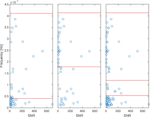
Figure 1: Illustration of the major steps in automated band selection. (The data realization used here is the first among the set described in Sec. V.1.) The left and middle panels show sources identified by xBSE using two different sets of frequency band edges (red lines). The right panel shows the union of the two sets of sources after the merging of sufficiently close sources and the band edges (red lines) obtained from the second and third largest gaps in the sorted set of source frequencies. The horizontal and vertical axes show the estimated SNR and frequencies of the sources, respectively.

IV.3 Cross-validation

One of the key components of SAPTARISHI is a step that we call cross-validation. The basic idea in cross-validation is that of comparing the identified sources obtained from two different algorithms in order to mitigate spurious ones. The details of the implementation are as follows.

Having obtained frequency bands as explained above, both xBSE and iBSE are applied to the data using the same set of bands. (To save computational cost, iBSE is initialized using the sources identified with xBSE.) This yields two semi-independent sets of identified sources $\Theta_{\rm xBSE}$ and $\Theta_{\rm iBSE}$ that, one expects, will have true sources in common but not spurious ones. A user-defined threshold $\eta_{\rm snr}$ is applied to both sets such that identified sources with estimated ${\rm SNR}<\eta_{\rm snr}$ are discarded. (The modified sets continue to be denoted as $\Theta_{\rm xBSE}$ and $\Theta_{\rm iBSE}$.)

Next, for each source $\theta\in\Theta_{\rm iBSE}$, the best match source $\theta^{\prime}\in\Theta_{\rm xBSE}$ is found (c.f., Sec. III.2). If, for a preset threshold $\eta_{\rm cv}$, $R_{\rm av}(\theta,\theta^{\prime})<\eta_{\rm cv}$, $\theta$ is removed from $\Theta_{\rm iBSE}$. The final list of the survivors in $\Theta_{\rm iBSE}$ constitute the set of reported sources from SAPTARISHI.

Figure 2 illustrates the effect of cross-validation. Identified sources from xBSE and iBSE become progressively weaker in SNR as the iterations proceed. Eventually, the identified sources get affected by confusion noise arising from unresolvable sources and are more likely to be spurious in nature. As can be seen from the figure, the estimated parameters of stronger sources show a good match between the two methods but the weaker sources do not always coincide. (Here, for visual clarity, we have used an ad hoc boundary of ${\rm SNR}=20$ to separate identified sources into weak and strong.) Cross-validation leverages this observation to filter out spurious sources. This can be seen in the way that it predominantly targets the weaker sources for removal and spares most of the stronger ones.

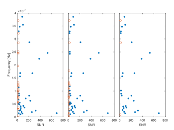
Figure 2: Illustration of cross-validation. The left and middle panels show sources identified by xBSE and iBSE, respectively, while the right panel shows the sources that survive after the cross-validation step. Open circles in each of the panels show sources with estimated ${\rm SNR}<20$ while filled circles show the rest. The horizontal and vertical axes show the estimated SNR and frequencies of the identified sources, respectively.

IV.4 The SAPTARISHI pipeline

We summarize here the complete SAPTARISHI pipeline here, starting with the list of its user-defined parameters.

• $N_{\rm ise}$: The number of iterations of vanilla-ISE in each frequency band.

• $p$: The number of sub-loudest sources subtracted in each step of iBSE.

• $\eta_{\rm band}$: The threshold used in automated frequency band selection for merging sufficiently close sources.

• $\eta_{\rm snr}$: The threshold on estimated ${\rm SNR}$ used to discard identified sources prior to cross-validation.

• $\eta_{\rm cv}$: The threshold used in cross-validation to reject identified sources that do not have well-matched counterparts across xBSE and iBSE.

In addition to the above parameters are the ones for PSO. In our experience with PSO in GW data analysis problems, we typically need to tune only two parameters in order to get good performance: the number of iterations ($N_{\rm iter}$) in one run of PSO, and the number of independent runs ($N_{\rm runs}$) of PSO on a given optimization task. The rest of the parameters involved in PSO are described in 2015ApJ…815..125W ; wangCoherentMethodDetection2014 and are kept at the same values. We set $N_{\rm iter}=2000$ and $N_{\rm runs}=8$ throughout this paper as this setting gives excellent performance while keeping computational costs manageable.

The steps involved in the SAPTARISHI pipeline are summarized below in sequential order.

1. Automated band selection.– This step is described in Sec. IV.2. It requires two separate runs of xBSE with two different sets of frequency bands. Note that within each search band, the sources are identified using vanilla-ISE.

2. xBSE.– This step uses the bands selected in the previous step and follows the description in Sec. IV.1.

3. iBSE.– The initialization of this step is carried out with the sources found in the previous step and follows the description in Sec. IV.1.

4. SNR threshold.– Identified sources from both xBSE and iBSE that have an estimated SNR below $\eta_{\rm snr}$ are discarded.

5. Cross validation.– This step, described in Sec. IV.3, is carried out on the identified sources that survive the SNR threshold above.

The final set of sources (i.e., reported sources) is the principal output of the pipeline. Note that, as per the terminology in Sec. III, this implies that the estimated values for all the signal parameters are obtained for each reported source. For simulated PTA data, one can proceed further to test for associations between the reported and true sources. This test simply follows the procedure described in Sec. III.2.

V Results

We begin this section with a description of our setup for simulating a large-scale PTA and its data. This is followed by the metrics we use to characterize the performance of SAPTARISHI and the presentation of our results.

V.1 Simulation setup and SAPTARISHI settings

We use two types of simulated PTAs, a mid-scale and a large-scale one, along with different numbers of GW sources to generate our simulated data realizations. The MSPs in both PTAs are selected from the synthetic catalog provided in 2009A&A…493.1161S based on simulated SKA pulsar surveys: the large-scale PTA has $10^{3}$ pulsars within $3$ kpc from Earth; the mid-scale one has the closest $10^{2}$ pulsars in the large-scale PTA.

Figure 3 shows the sky distribution of the pulsars in the above two PTAs. The main difference between the mid- and large-scale PTAs is the concentration of pulsars around the galactic plane. For the former, the pulsars are distributed more uniformly around the sky, which should lead to a different distribution of per-pulsar SNR values for randomly placed GW sources.

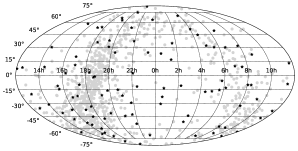
Figure 3: The sky distribution, in RA and Dec, of the pulsars in the simulated PTAs. The gray dots and black asterisks mark the locations of the pulsars in the large and mid-scale PTAs respectively.

The timing residual for each pulsar is simulated following the data model in Sec. II.1. The noise standard deviation is set uniformly for all pulsars to $100$ nsec, which is a conservative estimate of the timing error that is expected in SKA-era observations. The observation times for all timing residuals are identical across a given PTA and have a cadence of 1 sample per $2$ weeks. The total duration of the data is $5$ yr.

The number of GW sources for the large-scale PTA data is set to $200$ while it is $100$ for the mid-scale one. We generate $6$ independent data realizations, $\mathcal{Y}_{1}$ to $\mathcal{Y}_{6}$, as follows. Realizations $\mathcal{Y}_{1}$ to $\mathcal{Y}_{5}$ correspond to the large-scale PTA while $\mathcal{Y}_{6}$ corresponds to the mid-scale one. The latter is identical to the data used in songshengSearchContinuousGravitationalwave2021 . In all realizations, the GW source parameters $\alpha\in[0,2\pi]$, $\cos\delta\in[-1,1]$, $\psi\in[0,\pi]$, $\varphi_{0}\in[0,2\pi]$, $\log_{10}(f_{\rm gw})\in[0,\log_{10}(4.1\times 10^{-7})]$, and $\log_{10}(M)\in[6,10]$ ($M$ is the chirp mass of the SMBHB) are drawn independently from uniform distributions over their respective ranges. The distribution of the GW sources in distance corresponds to a constant spatial density up to a maximum of $10^{3}$ Mpc. In $\mathcal{Y}_{1}$ to $\mathcal{Y}_{4}$, $\iota$ is drawn from a uniform distribution on $[0,\pi]$, while in $\mathcal{Y}_{5}$ and $\mathcal{Y}_{6}$ the uniform distribution is over $\cos\iota\in[-1,1]$. The different distributions of $\iota$ affect the SNR distributions of GW signals by changing their polarization: $\iota=0$ and $\pi/2$ correspond to circulary and lineary polarized signals, respectively, with intermediate polarizations for other values. This provides a simple diagnostic of the robustness of a multisource resolution method against variations in the SNR distribution.

While the above distribution for the source population does not match the expected ones, such as sesanaSelfConsistentModel2010 , from realistic simulations, it is adequate for investigating the performance of multisource resolution methods. It has all the principal features, namely a higher density of sources at lower frequencies and lower SNRs, that are required to stress test data analysis methods.

The user-defined parameters of SAPTARISHI are listed in Sec. IV.4. For the results presented here, we set $N_{\rm ise}=20$, $p=5$, $\eta_{\rm band}=0.8$, $\eta_{\rm snr}=7.0$, and $\eta_{\rm cv}=0.7$. The value chosen for $\eta_{\rm snr}$ is based on the SNR distribution of identified sources, as shown in Fig. 4, obtained using data realizations containing only noise. We set $\eta_{\rm snr}=7.0$ as this is the closest round value to the $95$-th percentile (${\rm SNR}=7.13$) of this distribution. One expects that most identified sources at or below this SNR would be spurious.

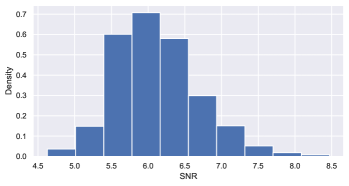
Figure 4: Distribution of SNR for identified sources obtained from noise-only data using vanilla-ISE. To obtain this distribution, $50$ independent realizations of noise-only PTA data were analyzed with $20$ iterations of vanilla-ISE per data realization. There was no division of the full frequency search range into smaller bands. This yields a total of $10^{3}$ identified sources in all.

V.2 Performance metrics

We use the following quantities to characterize the source resolution performance of SAPTARISHI on the simulated data described above. (i) Detection rate.– Let the set of reported sources and the set of true sources be $\Theta_{\rm rep}$ and $\Theta_{\rm true}$, respectively. For each reported source $\theta\in\Theta_{\rm rep}$ the best match source $\theta^{\prime}\in\Theta_{\rm true}$ with ${\rm SNR}>5.0$ is found. If, $R_{\rm av}(\theta,\theta^{\prime})\geq\eta_{\rm conf}$, where $\eta_{\rm conf}$ is a preset threshold, $\theta$ is admitted into the set, $\Theta_{\rm conf}$, of confirmed sources. The detection rate is $n(\Theta_{\rm conf})/n(\Theta_{\rm rep})$ expressed as a percentage. (ii) Lowest confirmed SNR.– This is the lowest estimated SNR in $\Theta_{\rm conf}$. We present results for $\eta_{\rm conf}\in\{0.65,0.70\}$ to characterize the variation in performance due to this user-defined parameter.

To quantify estimation performance, we consider differences in the values of signal parameters for matched pairs of confirmed and true sources. (While we will loosely refer to these differences as errors, it should be noted that they are not the same as the Frequentist or Bayesian notions of estimation error that always refer to a single true source.) In this paper, we restrict attention to parameters of astrophysical importance, namely, SNR, $f_{\rm gw}$, RA($\alpha$) and Dec($\delta$).

For SNR and $f_{\rm gw}$, we use the absolute relative difference defined as $\Delta\chi=|\chi_{\rm conf}-\chi_{\rm true}|/\chi_{\rm true}$, with $\chi$ denoting one these parameters and the subscript on $\chi$ denoting the set $\Theta_{\rm conf}$ or $\Theta_{\rm true}$ that a source belongs to. For the error in sky location, we use the shortest geodesic distance kellsPlaneSphericalTrigonometry , $d_{g}$, on the unit sphere between a matching pair of confirmed and true source. (We normalize $d_{g}$ by $2\pi$, the circumference of a great circle on the unit sphere.) The set of errors for all confirmed sources is visualized as an empirical survival rate curve $s(\epsilon)$. Here, $\epsilon$ is the estimation error ($\Delta\chi$ or $d_{g}/(2\pi)$) as described above and $s(\epsilon)$ is the fraction of confirmed sources that have a higher error than $\epsilon$.

V.3 Source resolution performance

Figure 5 shows the true sources used in all of the data realizations, $\mathcal{Y}_{1}$ to $\mathcal{Y}_{6}$, along with the reported sources from SAPTARISHI for each. We have chosen SNR and source frequency as the variables to display for each data realization. The former shows the large range of true source SNRs that was used in each data realization while the latter shows that, in common with more realistic SMBHB population models, there is increasing crowding of sources towards lower frequencies. As a result, one expects that source resolution would worsen as one goes to lower frequencies.

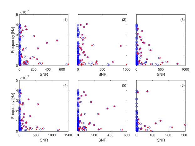
Figure 5: True (circles) and reported (dots) sources for the data realizations $\mathcal{Y}_{1}$ to $\mathcal{Y}_{6}$. The data realization corresponding to each panel is indicated by the number in parentheses at the top right corner.

The source resolution performance of SAPTARISHI is summarized in Table 1. There are two parts to this table and they differ only in the value of $\eta_{\rm conf}$ (c.f., Sec. V.2) used in the confirmation of reported sources. As can be seen from the table, lowering $\eta_{\rm conf}$ naturally admits more of the reported sources into the set of confirmed ones, thereby increasing the detection rate and finding weaker sources. However, this also allows more spurious sources to get through. Note that confirming a weaker source with lower $\eta_{\rm conf}$ does not necessarily imply that its parameters are well-matched to its corresponding true source. This worsens parameter estimation performance, as is discussed later in Sec. V.4. In either case, we see that SAPTARISHI delivers good performance in source resolution: for the higher $\eta_{\rm conf}$ and more stringent cut on reported sources, the detection rate stays above $78\%$, reaching its highest value of $93.3\%$ for $\mathcal{Y}_{6}$; for the lower $\eta_{\rm conf}$, the detection rate is above $\simeq 85\%$ in all cases and reaches $100\%$ for $\mathcal{Y}_{6}$.

(a) $\eta_{\rm conf}\geq 0.65$
Data realization	No. reported sources	Detection rate ($\%$)	Lowest SNR (Confirmed)
$\mathcal{Y}_{1}$	30	96.7	16.50
$\mathcal{Y}_{2}$	33	84.8	31.04
$\mathcal{Y}_{3}$	31	93.5	21.05
$\mathcal{Y}_{4}$	26	88.5	18.28
$\mathcal{Y}_{5}$	32	90.6	8.86
$\mathcal{Y}_{6}$	15	100	9.07
(b) $\eta_{\rm conf}\geq 0.70$
Data realization	No. reported sources	Detection rate ($\%$)	Lowest SNR (Confirmed)
$\mathcal{Y}_{1}$	30	86.7	18.64
$\mathcal{Y}_{2}$	33	78.8	31.04
$\mathcal{Y}_{3}$	31	87.1	22.10
$\mathcal{Y}_{4}$	26	84.6	18.28
$\mathcal{Y}_{5}$	32	78.1	16.43
$\mathcal{Y}_{6}$	15	93.3	9.07

Table 1: Source resolution performance of SAPTARISHI. The two parts, (a) and (b), correspond to different choices for the threshold $\eta_{\rm conf}$ used for confirming a given reported source.

The results for $\mathcal{Y}_{6}$ allow a direct comparison between the ISE approach of SAPTARISHI and the global fit approach used in songshengSearchContinuousGravitationalwave2021 . In the latter, the DNest method was able to resolve $8$ to $9$ sources with ${\rm SNR}\gtrsim 25$. From Table 1 for $\eta_{\rm conf}=0.7$, we see that SAPTARISHI resolves $14$ confirmed sources with the lowest ${\rm SNR}=9.07$.

It is interesting to analyze the effect of cross-validation on source resolution performance. If this step is removed from the pipeline (c.f., Sec. IV.4), we are left with separate sets of reported sources from xBSE and iBSE obtained by simply putting the threshold, $\eta_{\rm snr}\geq 7$, on the SNR of identified sources from each. Table 2 shows the results: Compared to part (b) of Table 1, there is a clear worsening of the detection rates, with steep drops for some of the data realizations such as $\mathcal{Y}_{1}$ and $\mathcal{Y}_{4}$.

Sometimes high SNR sources are missed due to confusion arising from the chance clustering of multiple sources in frequency. This happens more at low frequencies where sources are more crowded. One way in which we have observed the manifestation of confusion is when a cluster of sources are close in both frequency and SNR such that they collectively mimic a spurious high SNR source. When this spurious source is estimated and removed from the data, the power of each constituent source in the cluster is also reduced, making it undetectable in the latter iterations. This mechanism is most clearly seen for data realization $\mathcal{Y}_{2}$ in Fig. 5 where there is a spurious source at SNR $\approx 10^{3}$ that arises from the chance clustering of two sources with SNRs of $\approx 600$. The subtraction of the spurious source suppresses the detection of the latter two. The effect of confusion is smaller in $\mathcal{Y}_{6}$ due to the smaller number of sources. This explains why the detection rate is higher for this data realization.

(a) xBSE
Data realization	No. reported sources	Detection rate ($\%$)	Lowest SNR (Confirmed)
$\mathcal{Y}_{1}$	59	42.4	18.39
$\mathcal{Y}_{2}$	40	67.5	20.10
$\mathcal{Y}_{3}$	40	67.5	20.62
$\mathcal{Y}_{4}$	60	36.7	18.69
$\mathcal{Y}_{5}$	40	60	15.72
$\mathcal{Y}_{6}$	22	63.6	9.00
(b) iBSE
Data realization	No. reported sources	Detection rate ($\%$)	Lowest SNR (Confirmed)
$\mathcal{Y}_{1}$	59	49.2	18.64
$\mathcal{Y}_{2}$	40	70	31.04
$\mathcal{Y}_{3}$	40	80	22.10
$\mathcal{Y}_{4}$	60	43.3	18.28
$\mathcal{Y}_{5}$	40	65	16.43
$\mathcal{Y}_{6}$	19	84.2	7.56

Table 2: Source resolution performance without the cross-validation step. Reported sources are obtained separately from (a) xBSE and (b) iBSE using an SNR threshold $\eta_{\rm snr}\geq 7.0$ on identified sources. In both cases, the resulting reported sources are confirmed if $\eta_{\rm conf}\geq 0.7$.

V.4 Parameter estimation performance

Figures 6 and 7 show the sky distributions of true and reported sources for all the data realizations. For these plots, the reported sources correspond to part (b) of Table 1 with the threshold for elevating a reported source to confirmed set at the more stringent value of $\eta_{\rm conf}=0.7$. It is evident that the localization errors are small in general, even at lower SNRs. This is highly encouraging for the prospects of multi-messenger astronomy with large-scale PTAs in the scenario where SMBHBs are first identified using gravitational waves and then followed up in the electromagnetic window.

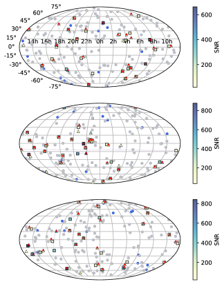
Figure 6: The sky distribution, in RA and Dec, of true, reported, and confirmed sources for data realizations $\mathcal{Y}_{1}$ to $\mathcal{Y}_{3}$ in order from top to bottom. In each plot, triangles show reported sources, stars represent confirmed sources, squares show true sources that matched a confirmed source, blue filled circles are true sources above the lowest confirmed SNR that were not detected, and filled gray circles show all other true sources. There is a dashed line joining each matching pair of confirmed and true sources but, the localization error being small in general, these lines are clearly visible only in a few instances. There is a long dashed line in the panel for $\mathcal{Y}_{2}$ but it actually connects a pair of sources that are quite close on the sphere. The triangle and square markers are shaded according to the estimated and true SNRs, respectively. The colorbar on the right of each panel shows the correspondence between the colors and SNRs.

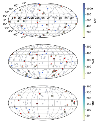
Figure 7: The sky distribution, in RA and Dec, of true, reported, and confirmed sources for data realizations $\mathcal{Y}_{4}$ to $\mathcal{Y}_{6}$ in order from top to bottom. The description of markers, colors, etc., is the same as for Fig. 6.

The errors in sky localization, SNR, and $f_{\rm gw}$ are further quantified in Fig. 8 using survival rate curves as described in Sec. V.2. Here, we only consider data realizations $\mathcal{Y}_{1}$ to $\mathcal{Y}_{5}$ since $\mathcal{Y}_{6}$ is drawn from a very different model. Instead, we provide summary statistics for it in Table 3. In Fig. 8, the principal survival curves correspond to $\eta_{\rm conf}=0.7$ but we also show the ones for $\eta_{\rm conf}=0.65$ to simply illustrate the point discussed earlier lowering $\eta_{\rm conf}$ increases detection rates but worsens parameter estimation.

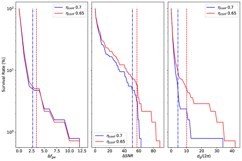
Figure 8: Survival rate curves for the errors (expressed as percentage) in $f_{\rm gw}$, SNR, and sky localization. The latter is quantified using the normalized shortest geodesic distance $d_{g}/(2\pi)$. The curves in blue and red correspond to different choices for $\eta_{\rm conf}$, the threshold used to elevate a reported source to a confirmed one. Corresponding to each curve, a vertical dashed line of the same color shows the $95$th percentile of the error distribution. Their specific values are as follows. For $\eta_{\rm conf}=0.7$, $\Delta f_{\rm gw}=2.7\%$, $\Delta{\rm SNR}=51.19\%$, and $d_{g}/(2\pi)=4.425\%$. For $\eta_{\rm conf}=0.65$, $\Delta f_{\rm gw}=3.44\%$, $\Delta{\rm SNR}=57.46\%$, and $d_{g}/(2\pi)=10.1\%$.

	$\Delta{\rm SNR}$	$\Delta f_{\rm gw}$	$d_{g}/(2\pi)$
Mean	8.71%	0.77%	0.87%
Minimum	0.19%	0	0.09%
Maximum	35.77%	5.09%	3.62%

Table 3: Summary statistics for the parameter estimation performance of SAPTARISHI on data realization $\mathcal{Y}_{6}$. Each column shows the sample mean, minimum and maximum values of the errors, as defined in Sec. V.2, for the parameter indicated in the heading of that column.

Not surprisingly, and in line with Fisher information analysis, $f_{\rm gw}$ is the most precisely determined parameter because it is the one that the likelihood function is most sensitive to. While a large fraction of sources are localized to within $10\%$ of a complete great circle emanating from a true source, there are a few large outliers. The number of these outliers grows as the threshold for confirmation, $\eta_{\rm conf}$, is lowered because more spurious reported sources manage to enter the set of confirmed sources.

The parameter estimation performance of SAPTARISHI for $\mathcal{Y}_{6}$ (c.f., Table 3) compares well with the global fit approach in songshengSearchContinuousGravitationalwave2021 . Here, it should be emphasized that the notion of error is different in frequentist and Bayesian methods: while SAPTARISHI provides a point estimate of parameters, with the inference of errors requiring a separate analysis using multiple data realizations, the DNest method provides samples from the joint (or marginalized) posterior probability density function of the parameters for a single data realization. Nonetheless, a comparison of our results for $\mathcal{Y}_{6}$ in Fig. 7 with Fig. 4 of songshengSearchContinuousGravitationalwave2021 shows that the errors in sky localization are similar in size.

V.5 Computational considerations

The current code for SAPTARISHI is a mix of Matlab and C language codes. For computational efficiency, the core routines, which includes MaxAvPhase, are all in the latter language. The overall computational cost is dominated by the vanilla-ISE runs required in automated frequency band selection, xBSE and iBSE. Essentially all of the cost of vanilla-ISE resides in the PSO-based optimization required in MaxAvPhase.

The runtime of SAPTARISHI is reduced considerably by exploiting the parallelism inherent to many of its components. The runs of vanilla-ISE on separate frequency bands are carried out in parallel on different compute nodes of a cluster. The multiple PSO runs required in MaxAvPhase execute in parallel on the processing cores of a single node. As a result, the runtime for vanilla-ISE on a given frequency band is simply the time required to execute MaxAvPhase with one PSO run – about 1 hour for the large-scale PTA on an Intel Xeon Platinum 8160 processor with a $2.1$ GHz clock rate – multiplied by the number of sources to be identified. Given that we have set the latter at $20$ in this paper, it takes about 20 hours for one vanilla-ISE run to finish on one frequency band. The total time taken to do one complete run of SAPTARISHI on one data realization then depends on how many vanilla-ISE runs are used in total.

At present, however, the number of vanilla-ISE runs is not a realistic predictor of the total time for a complete run. This is because the current structure of the SAPTARISHI code requires multiple jobs to run sequentially on a shared computing resource and each job incurs an unpredictable wait time in the queue. As we did not separately track the wait times, we can only report here that it typically takes about a week at present to analyze one data realization completely.

There is considerable scope for vastly speeding up SAPTARISHI that has not been tapped yet. Each iteration of PSO uses multiple independent evaluations of the function to be optimized and parallelizing over these can lead to a substantial reduction (about a factor of $\simeq 40$) in runtime. It is also possible in the case of MaxAvPhase to implement parallelization within a single function evaluation with hardware-level acceleration using Graphics Processing Units (GPUs) or multi-threaded numerical libraries. This could easily bring in another factor of $O(10)$. We plan to implement these nested layers of parallelization in the future. (Substantially speeding up the code will also help mitigate the problem of wait times if the complete run could be executed as a single job within the maximum time allowed for a job.)

VI Conclusions

We have introduced SAPTARISHI, a method for resolving SMBHB sources in data from PTAs. The method uses an ISE approach and performs well relative to the global fit methods that have been proposed for the PTA multisource resolution problem. It is scalable to PTAs with a large number of pulsars and its application to simulated data demonstrates that the source confusion problem for future large-scale PTAs is solvable.

SAPTARISHI was applied to two types of PTAs, a large-scale one with $10^{3}$ pulsars and a mid-scale one with $10^{2}$ pulsars. Detection rates above $\simeq 78\%$ were achieved in all cases. The lowest confirmed SNR for the large and mid-scale PTAs reached $16.43$ and $9.07$, respectively. Note that, assuming a naive $\sqrt{N_{\rm p}}$ scaling of SNR with the number of pulsars, the source with the lowest confirmed SNR for the large-scale PTA would have an SNR of only $\simeq 5.2$ for the mid-scale one, making it too weak to resolve with the latter. This indicates the usefulness of a larger number of array pulsars for not only improving single source search sensitivity 2017PhRvL.118o1104W but also multisource resolvability.

The levels of lowest confirmed SNR above bode well for the ability of a future large-scale PTA to peer far back into the Universe. For example, using the lowest confirmed SNR of $16.43$ as a reference and an observation period of 5 yr, a SMBHB with $f_{\rm gw}=2\times 10^{-8}$ Hz and redshifted chirp mass of $10^{9}~{}M_{\odot}$ ($10^{10}~{}M_{\odot}$) will be located at a redshift of $z=0.24$ ($z=5.84$) or a luminosity distance (standard cosmology) of $1.23$ Gpc ($57.3$ Gpc). [The corresponding chirp mass in the source frame is $8\times 10^{8}~{}M_{\odot}$ ($1.5\times 10^{9}~{}M_{\odot}$).] Here, we have used the relation in 2017PhRvL.118o1104W between redshift, or distance, and the SNR averaged over the geometrical factors that occur in the response of the large-scale PTA.

The successes of both the ISE and global fit approaches suggest that the strengths of the two can be combined to create an approach that is more powerful. For example, a weakness of the ISE approach is that the proximity of two sources in frequency leads to an overestimate, due to their overlap, of the louder SNR and an underestimate of the weaker one when the louder is subtracted out. On the other hand, as shown in PhysRevD.85.044034 , a global fit approach can estimate some source parameters accurately even if the sources coincide in frequency.

Similarly, a weakness of the global fit approach is the necessity of assuming the number of sources and then using some form of model selection to find the best number. Finding the global fit becomes harder as the dimensionality of the combined parameter space increases with the number of sources, requiring special measures to combat this effect. An ISE approach does not need the number of sources and can identify as many as required. As shown in this paper, post-processing steps such as cross-validation can then be used to weed out a large fraction of spurious sources. It is conceivable that the number of reported sources from the ISE approach provides a good initial estimate for a global fit approach.

The synergy of the ISE and global fit approaches described above, as well as additional ones, will be explored in future work. Code modifications outlined in the paper to make SAPTARISHI substantially faster are in progress. This will allow its detection and estimation performance to be quantified more thoroughly using a much larger set of data realizations.

A limitation of the current code is the use of the white noise model. While appropriate for the development of data analysis methods, effects such as red noise and timing model errors (c.f., Sec. II.1) need to be included in order to analyze real data. The key components of SAPTARISHI, namely xBSE, iBSE, and cross-validation, use the estimated source waveforms and parameters produced by the single-source estimation method, MaxAvPhase, as inputs. Thus, these steps are independent of the details of the single source method, allowing it to be substituted easily with any other method in the future that incorporates a more sophisticated noise model.

Red noise: Under the likely scenario that individual timing residuals are noise dominated, the covariance matrix of the noise, including red noise, can be estimated from the data. This estimate can then be fed into the log-likelihood. Alternatively, a parametrized model for the covariance matrix can be used and the parameters estimated jointly with those of the signal. Since both MaxPhase and AvPhase are derived from the log-likelihood, the modifications required are, in principle, straightforward and the computational burden is likely to increase only modestly.

Timing model errors: For incorporating timing model errors, the standard approach uses a linear model with unknown coefficients 1984JApA….5..369B . In general, the log-likelihood for Gaussian noise is a convex function over linear parameters. We expect the log-likelihood maximized or marginalized over the pulsar phase parameters to retain a similar simple structure over these parameters. Therefore, it is likely that with a suitable nested maximization scheme, in which the timing model error parameters are maximized over first, the optimization by PSO of the log-likelihood over the larger set of intrinsic parameters remains feasible albeit with a higher computational cost. Further work is in progress on this topic.

Appendix A AvPhase

Following 2015ApJ…815..125W , for a PTA of $N_{\rm p}$ pulsars, the log-likelihood ratio is

$$\ln\Lambda(\mathcal{Y};\lambda) = \sum_{I=1}^{N_{\rm p}}\ln\Lambda_{I}({\overline{y}^{I}};\lambda)\,,$$ (13)

where for the $I$-th pulsar,

$$\ln\Lambda_{I}(\overline{y}^{I};\lambda) =\left[\left\langle\overline{y}^{I}\mid X_{I}\right\rangle_{I}\cos 2\phi_{I}+\left\langle\overline{y}^{I}\mid Y_{I}\right\rangle_{I}\sin 2\phi_{I}\right.$$ (14)

$$+\left\langle\overline{y}^{I}\mid Z_{I}\right\rangle_{I}-\frac{1}{2}\left(\left\langle X_{I}\mid X_{I}\right\rangle_{I}\cos^{2}2\phi_{I}\right.$$

$$+\left\langle Y_{I}\mid Y_{I}\right\rangle_{I}\sin^{2}2\phi_{I}+2\left\langle X_{I}\mid Y_{I}\right\rangle_{I}\sin 2\phi_{I}\cos 2\phi_{I}$$

$$+2\left\langle X_{I}\mid Z_{I}\right\rangle_{I}\cos 2\phi_{I}+2\left\langle Y_{I}\mid Z_{I}\right\rangle_{I}\sin 2\phi_{I}$$

$$\left.\left.+\left\langle Z_{I}\mid Z_{I}\right\rangle_{I}\right)\right].$$

Here the explicit expressions of $X_{I}$, $Y_{I}$ and $Z_{I}$ can be found in 2015ApJ…815..125W .

AvPhase marginalizes the likelihood ratio over the pulsar phase parameters (c.f., Sec. II.1) and maximizes the resulting function over the remaining parameters. This creates a new detection statistic, which we call Marginalized-Maximized Likelihood Ratio Test, 2017JPhCS.840a2058W given by

$$\text{MMLRT}(\mathcal{Y})=\max_{\lambda_{i}}\ln\left(\rm marg_{\lambda_{e}}\Lambda(\mathcal{Y};\lambda)\right)\,,$$ (15)

where marg denotes the marginalization operation. Here, the maximization over intrinsic parameters $\lambda_{i}$ is handled by PSO while the marginalization over the extrinsic parameters $\lambda_{e}$ is handled by numerical integration.

The marginalization over the set of pulsar phase parameters, $\{\phi_{I}\}$, $I=1,2,\ldots,N_{\rm p}$, in Eq. 15 is similar in spirit to existing proposals in Bayesian approaches to SMBHB search but differs significantly in implementation. In 2013CQGra..30v4004E , marginalization over $\{\phi_{I}\}$ (and other parameters) is performed on the estimated posterior probability density function (PDF), obtained with an MCMC based method, defined on the full parameter space of a single source. Note that this is not the same as sampling a posterior that is already marginalized over $\{\phi_{I}\}$ since the dimensionality of the parameter space explored by MCMC is vastly different in the two cases. The substantial computational cost of MCMC based estimation of the posterior PDF defined over the full parameter space makes this approach ill-suited for scaling to SKA-era PTAs. In 2014PhRvD..90j4028T , a solution was proposed in the form of direct numerical integration of the posterior over $\{\phi_{I}\}$, carried out at each iteration of the MCMC method. While this reduces the computational cost, the time to convergence of the numerical integration method reportedly varies a lot with the SNR of the injected signal since it affects the shape of the posterior in the $N_{\rm p}$-dimensional space of $\{\phi_{I}\}$. In AvPhase, the marginalization of the likelihood over pulsar phases is performed economically using $N_{\rm p}$ decoupled one-dimensional integrations that, as described below, are carefully crafted to avoid numerical issues and incur a (nearly) fixed computational cost.

A.1 Marginalization over pulsar phases

To compute MMLRT one can rewrite the log-likelihood ratio function, i.e. Eq. 14, in the following form:

$$\ln\Lambda_{I}(\overline{y}^{I};\lambda)= b_{1}+b_{2}\cos 2\phi_{I}+b_{3}\sin 2\phi_{I}+$$ (16)

$$b_{4}\sin 2\phi_{I}\cos 2\phi_{I}+b_{5}\cos^{2}2\phi_{I}+$$

$$b_{6}\sin^{2}2\phi_{I}\,.$$

Here, $b_{1}=\langle\overline{y}^{I}\mid Z_{I}\rangle_{I}-\frac{1}{2}\langle Z_{I}\mid Z_{I}\rangle_{I}$, $b_{2}=\langle\overline{y}^{I}\mid X_{I}\rangle_{I}-\langle X_{I}\mid Z_{I}\rangle_{I}$, $b_{3}=\langle\overline{y}^{I}\mid Y_{I}\rangle_{I}-\langle Y_{I}\mid Z_{I}\rangle_{I}$, $b_{4}=-\langle X_{I}\mid Y_{I}\rangle_{I}$, $b_{5}=-\frac{1}{2}\langle X_{I}\mid X_{I}\rangle_{I}$, and $b_{6}=-\frac{1}{2}\langle Y_{I}\mid Y_{I}\rangle_{I}$. Note that we have suppressed the index $I$ of $b$’s for clarity. Thus, the likelihood ratio function $\Lambda_{I}=\exp(\ln\Lambda_{I})$ is

$$\Lambda_{I}(\overline{y}^{I};\lambda) =\exp(b_{1}+b_{2}\cos 2\phi_{I}+b_{3}\sin 2\phi_{I}$$ (17)

$$+b_{4}\sin 2\phi_{I}\cos 2\phi_{I}+b_{5}\cos^{2}2\phi_{I}+b_{6}\sin^{2}2\phi_{I})\,.$$

The marginalization of $\Lambda$ over the pulsar phases involves $N_{\rm p}$ decoupled integrations as follows

$$\Lambda_{I}(\overline{y}^{I};\lambda_{i}) =\int_{0}^{\pi}\exp(b_{1}+b_{2}\cos 2\phi_{I}+b_{3}\sin 2\phi_{I}$$ (18)

$$+b_{4}\sin 2\phi_{I}\cos 2\phi_{I}+b_{5}\cos^{2}2\phi_{I}$$

$$+b_{6}\sin^{2}2\phi_{I})~{}\text{d}\phi_{I}\,.$$

Set $x=2\phi_{I}$, then

$$\Lambda_{I}(\overline{y}^{I};\lambda_{i}) =\frac{1}{2}\int_{0}^{2\pi}\exp(b_{1}+b_{2}\cos x+b_{3}\sin x$$ (19)

$$+b_{4}\sin x\cos x+b_{5}\cos^{2}x+b_{6}\sin^{2}x)~{}\text{d}x\,.$$

Eq. 19 is equivalent to the marginalization of the posterior PDF in the Bayesian framework with a flat prior over $x$. For the special case $b_{4}=b_{5}=b_{6}=0$, the integration has a closed form solution in terms of the modified Bessel function of the first kind. In general though, Eq. 19 does not have a closed form solution and numerical integration must be used. While this appears straightforward, it turns out that the power of the exponential in the integrand can occasionally become very large (say $>10^{8}$), making the integrand exceed the dynamical range of floating point precision to become practically infinite. However, since what we really want is the logarithm of Eq. 19, we can mitigate this problem by factoring out the dominant part of the integrand as explained next.

A.2 Integration

One can regard $b$’s as the coefficients of the basis functions, i.e. ($1,\sin x,\cos x,\sin x\cos x,\cos^{2}x,\sin^{2}x$), which have ranges from -1 to 1. The largest absolute value of the terms will determine the factorization of the integration. And we note that the basis functions change their sign in each of the four quadrants of $[0,2\pi)$. To find out which term is dominating, we rewrite the integration as follows

$$\Lambda_{I}(\overline{y}^{I};\lambda_{i}) =\frac{1}{2}\sum_{k=1}^{4}\int_{l_{k}}^{u_{k}}\exp(b_{1}S_{k1}^{2}+b_{2}S_{k2}^{2}\cos x$$ (20)

$$+b_{3}S_{k3}^{2}\sin x+b_{4}S_{k4}^{2}\sin x\cos x$$

$$+b_{5}S_{k5}^{2}\cos^{2}x+b_{6}S_{k6}^{2}\sin^{2}x)~{}\text{d}x\,.$$

Here $S_{kl}$ is the element of the sign matrix

$$\mathbf{S}=\left(\begin{array}[]{cccccc}1&1&1&1&1&1\\ 1&-1&1&-1&1&1\\ 1&-1&-1&1&1&1\\ 1&1&-1&-1&1&1\\ \end{array}\right)\,.$$ (21)

$S_{kl}^{2}=1$. Thus, we can redefine the new coefficients in quadrant $k$ as $b_{sl}^{k}=S_{kl}b_{l}$, and the new basis functions in quadrant $k$ as $S_{kl}V_{l}$ which are always positive in each quadrant. (Note, the summation rule is not applied here.)

Therefore, Eq. 20 can be explicitly written as

$$\Lambda_{I}(\overline{y}^{I};\lambda_{i}) =\frac{1}{2}\int_{0}^{2\pi}\exp(f(x))~{}\text{d}x\,,$$ (22a)

$$=\frac{1}{2}\sum_{k=1}^{4}e^{6N_{k}}\int_{l_{k}}^{u_{k}}g_{k}(x)~{}\text{d}x\,,$$ (22b)

$$=\frac{1}{2}\sum_{k=1}^{4}e^{6N_{k}}\exp(\ln(R_{k}))\,.$$ (22c)

where $N_{k}=\max(b_{s}^{k})$, $R_{k}=\int_{l_{k}}^{u_{k}}g_{k}(x)~{}\text{d}x$. In quadrant $k$, the integration can be written as

$$\int_{l_{k}}^{u_{k}}\exp(f(x))~{}\text{d}x =\int_{l_{k}}^{u_{k}}\exp(b_{1}S_{k1}^{2}+b_{2}S_{k2}^{2}\cos x$$

$$+b_{3}S_{k3}^{2}\sin x+b_{4}S_{k4}^{2}\sin x\cos x$$

$$+b_{5}S_{k5}^{2}\cos^{2}x+b_{6}S_{k6}^{2}\sin^{2}x)~{}\text{d}x\,,$$ (23a)

$$=e^{6N_{k}}\int_{l_{k}}^{u_{k}}\exp(b_{s1}^{k}+b_{s2}^{k}|\cos x|$$

$$+b_{s3}^{k}|\sin x|+b_{s4}^{k}|\sin 2x\cos 2x|$$

$$+b_{s5}^{k}|\cos^{2}x|+b_{s6}^{k}|\sin^{2}x|-6N_{k})~{}\text{d}x\,.$$ (23b)

The exponent in Eq. 23b is well behaved (after subtracting $6N_{k}$, each term in the exponent should be less than one), therefore it can be integrated using the usual algorithms without special treatment.

To sum the contributions from the four quadrants, we define $M_{k}=6N_{k}+\ln R_{k}$, then

$$\Lambda_{I}(\overline{y}^{I};\lambda_{i})=\frac{1}{2}\sum_{k=1}^{4}\exp(M_{k})\,.$$ (24)

Set $\bar{M}=\max(M_{k})$, and $\tilde{M}_{k}=M_{k}-\bar{M}$,

$$\Lambda_{I}(\overline{y}^{I};\lambda_{i})=\frac{1}{2}\exp(\bar{M})\sum_{k=1}^{4}\exp(\tilde{M}_{k})\,,$$ (25)

$$\ln\Lambda_{I}(\overline{y}^{I};\lambda_{i})=\bar{M}+Q-\ln 2\,,$$ (26)

where $Q=\sum_{k=1}^{4}\exp(\tilde{M}_{k})$.

References

- (1) B. P. Abbott et al., “Observation of Gravitational Waves from a Binary Black Hole Merger,” Physical Review Letters, vol. 116, p. 061102, Feb. 2016.
- (2) B. P. Abbott et al., “GWTC-1: A Gravitational-Wave Transient Catalog of Compact Binary Mergers Observed by LIGO and Virgo during the First and Second Observing Runs,” Physical Review X, vol. 9, p. 031040, Jul 2019.
- (3) R. Abbott et al., “GWTC-2: Compact Binary Coalescences Observed by LIGO and Virgo During the First Half of the Third Observing Run,” arXiv e-prints, p. arXiv:2010.14527, Oct. 2020.
- (4) P. Amaro-Seoane et al., “Laser Interferometer Space Antenna,” arXiv e-prints, p. arXiv:1702.00786, Feb. 2017.
- (5) J. Luo et al., “TianQin: a space-borne gravitational wave detector,” Classical and Quantum Gravity, vol. 33, p. 035010, Feb. 2016.
- (6) W.-R. Hu and Y.-L. Wu, “The Taiji Program in Space for gravitational wave physics and the nature of gravity,” National Science Review, vol. 4, pp. 685–686, 10 2017.
- (7) S. Sato et al., “DECIGO: The Japanese space gravitational wave antenna,” Journal of Physics Conference Series, vol. 154, p. 012040, Mar. 2009.
- (8) K. A. Kuns, H. Yu, Y. Chen, and R. X. Adhikari, “Astrophysics and cosmology with a decihertz gravitational-wave detector: TianGO,” Phys. Rev. D, vol. 102, p. 043001, Aug. 2020.
- (9) L. Lentati et al., “European Pulsar Timing Array limits on an isotropic stochastic gravitational-wave background,” Monthly Notices of the Royal Astronomical Society, vol. 453, pp. 2576–2598, 08 2015.
- (10) R. M. Shannon et al., “Gravitational waves from binary supermassive black holes missing in pulsar observations,” Science, vol. 349, pp. 1522–1525, Sept. 2015.
- (11) Z. Arzoumanian et al., “The NANOGrav Nine-year Data Set: Limits on the Isotropic Stochastic Gravitational Wave Background,” Astrophys. J. , vol. 821, p. 13, Apr. 2016.
- (12) Z. Arzoumanian et al., “The NANOGrav 11 Year Data Set: Pulsar-timing Constraints on the Stochastic Gravitational-wave Background,” Astrophys. J. , vol. 859, p. 47, May 2018.
- (13) X.-J. Zhu et al., “An all-sky search for continuous gravitational waves in the Parkes Pulsar Timing Array data set,” Monthly Notices of the Royal Astronomical Society, vol. 444, pp. 3709–3720, Nov. 2014.
- (14) S. Babak et al., “European Pulsar Timing Array limits on continuous gravitational waves from individual supermassive black hole binaries,” Monthly Notices of the Royal Astronomical Society, vol. 455, pp. 1665–1679, Jan. 2016.
- (15) K. Aggarwal et al., “The NANOGrav 11 yr Data Set: Limits on Gravitational Waves from Individual Supermassive Black Hole Binaries,” Astrophys. J. , vol. 880, p. 116, Aug. 2019.
- (16) J. B. Wang et al., “Searching for gravitational wave memory bursts with the Parkes Pulsar Timing Array,” Monthly Notices of the Royal Astronomical Society, vol. 446, pp. 1657–1671, Jan. 2015.
- (17) K. Aggarwal et al., “The NANOGrav 11 yr Data Set: Limits on Gravitational Wave Memory,” Astrophys. J. , vol. 889, p. 38, Jan. 2020.
- (18) M. F. Alam et al., “The NANOGrav 12.5 yr Data Set: Observations and Narrowband Timing of 47 Millisecond Pulsars,” The Astrophysical Journal Supplement Series, vol. 252, p. 4, Jan. 2021.
- (19) M. F. Alam et al., “The NANOGrav 12.5 yr Data Set: Wideband Timing of 47 Millisecond Pulsars,” The Astrophysical Journal Supplement Series, vol. 252, p. 5, Jan. 2021.
- (20) Z. Arzoumanian et al., “The NANOGrav 12.5 yr Data Set: Search for an Isotropic Stochastic Gravitational-wave Background,” The Astrophysical Journal Letters, vol. 905, p. L34, Dec. 2020.
- (21) R. W. Hellings and G. S. Downs, “Upper limits on the isotropic gravitational radiation background from pulsar timing analysis.,” The Astrophysical Journal Letters, vol. 265, pp. L39–L42, Feb. 1983.
- (22) B. Goncharov et al., “On the evidence for a common-spectrum process in the search for the nanohertz gravitational-wave background with the parkes pulsar timing array,” The Astrophysical Journal Letters, vol. 917, p. L19, aug 2021.
- (23) S. Chen et al., “Common-red-signal analysis with 24-yr high-precision timing of the European Pulsar Timing Array: Inferences in the stochastic gravitational-wave background search,” Monthly Notices of the Royal Astronomical Society, 2021.
- (24) J. Antoniadis et al., “The International Pulsar Timing Array second data release: Search for an isotropic gravitational wave background,” Monthly Notices of the Royal Astronomical Society, vol. 510, pp. 4873–4887, Jan. 2022.
- (25) R. Nan et al., “The Five-Hundred Aperture Spherical Radio Telescope (fast) Project,” International Journal of Modern Physics D, vol. 20, pp. 989–1024, 2011.
- (26) G. Hobbs et al., “The role of FAST in pulsar timing arrays,” Research in Astronomy and Astrophysics, vol. 19, p. 020, Feb. 2019.
- (27) R. Smits et al., “Pulsar searches and timing with the square kilometre array,” Astronomy and Astrophysics, vol. 493, pp. 1161–1170, Jan. 2009.
- (28) G. Janssen et al., “Gravitational Wave Astronomy with the SKA,” in Advancing Astrophysics with the Square Kilometre Array (AASKA14), p. 37, Apr. 2015.
- (29) J. L. Han et al., “The FAST Galactic Plane Pulsar Snapshot survey: I. Project design and pulsar discoveries,” Research in Astronomy and Astrophysics, vol. 21, p. 107, June 2021.
- (30) SKA website: www.skatelescope.org.
- (31) G. Hobbs, S. Dai, R. N. Manchester, R. M. Shannon, M. Kerr, K.-J. Lee, and R.-X. Xu, “The role of FAST in pulsar timing arrays,” Research in Astronomy and Astrophysics, vol. 19, p. 020, feb 2019.
- (32) Y. Wang and S. D. Mohanty, “Pulsar Timing Array Based Search for Supermassive Black Hole Binaries in the Square Kilometer Array Era,” Phys. Rev. Lett., vol. 118, p. 151104, Apr 2017.
- (33) Y. Wang and S. D. Mohanty, “Erratum: Pulsar timing array based search for supermassive black hole binaries in the square kilometer array era [phys. rev. lett. 118, 151104 (2017)],” Phys. Rev. Lett., vol. 124, p. 169901, Apr 2020.
- (34) Y. Wang, S. D. Mohanty, and Z. Cao, “Extending the Frequency Reach of Pulsar Timing Array-based Gravitational Wave Search without High-cadence Observations,” The Astrophysical Journal Letters, vol. 907, p. L43, Feb. 2021.
- (35) J.-M. Wang and Y.-R. Li, “Observational signatures of close binaries of supermassive black holes in active galactic nuclei,” Research in Astronomy and Astrophysics, vol. 20, p. 160, Oct. 2020.
- (36) C. Xin, C. M. F. Mingarelli, and J. S. Hazboun, “Multimessenger Pulsar Timing Array Constraints on Supermassive Black Hole Binaries Traced by Periodic Light Curves,” Astrophys. J. , vol. 915, no. 2, p. 97.
- (37) M. J. Valtonen et al., “A massive binary black-hole system in OJ 287 and a test of general relativity,” Nature, vol. 452, pp. 851–853, Apr. 2008.
- (38) M. J. Graham et al., “A possible close supermassive black-hole binary in a quasar with optical periodicity,” Nature, vol. 518, pp. 74–76, Feb. 2015.
- (39) Y.-R. Li et al., “Spectroscopic Indication of a Centi-Parsec Supermassive Black Hole Binary in the Galactic Center of Ngc 5548,” Astrophys. J. , vol. 822, no. 1, p. 4.
- (40) Y.-R. Li et al., “A Possible 20 yr Periodicity in Long-term Optical Photometric and Spectral Variations of the Nearby Radio-quiet Active Galactic Nucleus Ark 120,” The Astrophysical Journal Supplement Series, vol. 241, p. 33, Apr. 2019.
- (41) J.-M. Wang et al., “Kinematic Signatures of Reverberation Mapping of Close Binaries of Supermassive Black Holes in Active Galactic Nuclei,” Astrophys. J. , vol. 862, p. 171, Aug. 2018.
- (42) Y.-Y. Songsheng, J.-M. Wang, and Y.-R. Li, “The VLT Interferometric Measurements of Active Galactic Nuclei: Effects of Angular Momentum Distributions of Clouds in the Broad-line Region,” Astrophys. J. , vol. 883, p. 184, Oct. 2019.
- (43) Z. Arzoumanian et al., “Multimessenger Gravitational-wave Searches with Pulsar Timing Arrays: Application to 3C 66B Using the NANOGrav 11-year Data Set,” Astrophys. J. , vol. 900, no. 2, p. 102.
- (44) T. B. Littenberg, “A detection pipeline for Galactic binaries in LISA data,” Phys. Rev. D, vol. 84, p. 063009, 2011.
- (45) A. Blaut, S. Babak, and A. Krolak, “Mock LISA Data Challenge for the Galactic white dwarf binaries,” Phys. Rev. D, vol. 81, p. 063008, 2010.
- (46) X.-H. Zhang et al., “Resolving galactic binaries in lisa data using particle swarm optimization and cross-validation,” Phys. Rev. D, vol. 104, p. 024023, Jul 2021.
- (47) A. Petiteau et al., “Resolving multiple supermassive black hole binaries with pulsar timing arrays. ii. genetic algorithm implementation,” Phys. Rev. D, vol. 87, p. 064036, Mar 2013.
- (48) S. Babak and A. Sesana, “Resolving multiple supermassive black hole binaries with pulsar timing arrays,” Phys. Rev. D, vol. 85, p. 044034, Feb 2012.
- (49) B. Bécsy and N. J. Cornish, “Joint search for isolated sources and an unresolved confusion background in pulsar timing array data,” Classical and Quantum Gravity, vol. 37, no. 13, p. 135011, 2020.
- (50) X. J. Zhu et al., “Detection and localization of continuous gravitational waves with pulsar timing arrays: the role of pulsar terms,” Monthly Notices of Royal Astronomical Society, vol. 461, pp. 1317–1327, Sept. 2016.
- (51) Y.-Y. Songsheng et al., “Search for Continuous Gravitational-wave Signals in Pulsar Timing Residuals: A New Scalable Approach with Diffusive Nested Sampling,” The Astrophysical Journal, vol. 922, p. 228, Dec. 2021.
- (52) N. J. Cornish and S. L. Larson, “Lisa data analysis: Source identification and subtraction,” Physical Review D, vol. 67, no. 10, p. 103001, 2003.
- (53) J. A. Högbom, “Aperture Synthesis with a Non-Regular Distribution of Interferometer Baselines,” Astronomy and Astrophysics Supplement, vol. 15, p. 417, June 1974.
- (54) J. Kennedy and R. C. Eberhart, ““Particle swarm optimization”,” in Proceedings of the IEEE International Conference on Neural Networks: Perth, WA, Australia, vol. 4, p. 1942, IEEE, 1995.
- (55) S. D. Mohanty, Swarm Intelligence Methods for Statistical Regression. Chapman and Hall/CRC, 2018.
- (56) Y. Wang, S. D. Mohanty, and F. A. Jenet, “Coherent Network Analysis for Continuous Gravitational Wave Signals in a Pulsar Timing Array: Pulsar Phases as Extrinsic Parameters,” Astrophys. J. , vol. 815, p. 125, Dec. 2015.
- (57) Y. Wang, S. D. Mohanty, and Y.-Q. Qian, “Continuous gravitational wave searches with pulsar timing arrays: Maximization versus marginalization over pulsar phase parameters,” in Journal of Physics Conference Series, vol. 840 of Journal of Physics Conference Series, p. 012058, May 2017.
- (58) R. T. Edwards, G. B. Hobbs, and R. N. Manchester, “TEMPO2, a new pulsar timing package - II. The timing model and precision estimates,” Monthly Notices of the Royal Astronomical Society, vol. 372, pp. 1549–1574, Nov. 2006.
- (59) R. Blandford, R. Narayan, and R. W. Romani, “Arrival-time analysis for a millisecond pulsar.,” Journal of Astrophysics and Astronomy, vol. 5, pp. 369–388, Dec. 1984.
- (60) Y. Wang, “Noise in pulsar timing arrays,” in Journal of Physics Conference Series, vol. 610 of Journal of Physics Conference Series, p. 012019, May 2015.
- (61) R. M. Shannon and J. M. Cordes, “Assessing the Role of Spin Noise in the Precision Timing of Millisecond Pulsars,” Astrophys. J. , vol. 725, pp. 1607–1619, Dec. 2010.
- (62) F. B. Estabrook and H. D. Wahlquist, “Response of Doppler spacecraft tracking to gravitational radiation.,” General Relativity and Gravitation, vol. 6, pp. 439–447, Oct 1975.
- (63) A. Sesana and A. Vecchio, “Measuring the parameters of massive black hole binary systems with pulsar timing array observations of gravitational waves,” Phys. Rev. D, vol. 81, p. 104008, May 2010.
- (64) K. J. Lee et al., “Gravitational wave astronomy of single sources with a pulsar timing array,” Monthly Notices of the Royal Astronomical Society, vol. 414, pp. 3251–3264, July 2011.
- (65) Y. Wang, S. D. Mohanty, and F. A. Jenet, “A Coherent Method for the Detection and Parameter Estimation of Continuous Gravitational Wave Signals Using a Pulsar Timing Array,” Astrophys. J. , vol. 795, p. 96, Nov. 2014.
- (66) J. A. Ellis, X. Siemens, and J. D. E. Creighton, “Optimal Strategies for Continuous Gravitational Wave Detection in Pulsar Timing Arrays,” Astrophys. J. , vol. 756, p. 175, Sept. 2012.
- (67) J. A. Ellis, “A Bayesian analysis pipeline for continuous GW sources in the PTA band,” Classical and Quantum Gravity, vol. 30, p. 224004, Nov. 2013.
- (68) Y. Wang and S. D. Mohanty, “RAAPTR (Repository of Analysis Algorithms for Pulsar Timing Residuals).” github.com/yanwang2012/RAAPTR, 2021.
- (69) B. B. P. Perera et al., “Improving timing sensitivity in the microhertz frequency regime: limits from PSR J1713+0747 on gravitational waves produced by supermassive black hole binaries,” Monthly Notices of the Royal Astronomical Society, vol. 478, pp. 218–227, July 2018.
- (70) T. Dolch et al., “Single-Source Gravitational Wave Limits From the J1713+0747 24-hr Global Campaign,” in Journal of Physics Conference Series, vol. 716 of Journal of Physics Conference Series, p. 012014, May 2016.
- (71) S. Yi et al., “Limits on the strength of individual gravitational wave sources using high-cadence observations of PSR B1937+21,” Monthly Notices of the Royal Astronomical Society, vol. 445, pp. 1245–1252, Dec 2014.
- (72) J. Crowder and N. J. Cornish, “Extracting Galactic binary signals from the first round of Mock LISA Data Challenges,” Classical and Quantum Gravity, vol. 24, pp. S575–S585, sep 2007.
- (73) S. D. Mohanty, “Median based line tracker (MBLT): Model independent and transient preserving line removal from interferometric data,” Classical and Quantum Gravity, vol. 19, pp. 1513–1519, Apr. 2002.
- (74) Y. Wang, S. D. Mohanty, and F. A. Jenet, “A Coherent Method for the Detection and Parameter Estimation of Continuous Gravitational Wave Signals Using a Pulsar Timing Array,” Astrophys. J. , vol. 795, no. 1, p. 96.
- (75) A. Sesana, “Self consistent model for the evolution of eccentric massive black hole binaries in stellar environments: implications for gravitational wave observations,” vol. 719, no. 1, pp. 851–864.
- (76) L. M. Kells, W. F. Kern, and J. R. Bland, Plane And Spherical Trigonometry. McGraw Hill Book Company, Inc.
- (77) S. Taylor, J. Ellis, and J. Gair, “Accelerated Bayesian model-selection and parameter-estimation in continuous gravitational-wave searches with pulsar-timing arrays,” Phys. Rev. D, vol. 90, p. 104028, Nov. 2014.