Photometric Redshift Estimation of BASS DR3 Quasars by Machine Learning

Abstract

Correlating BASS DR3 catalogue with ALLWISE database, the data from optical and infrared information are obtained. The quasars from SDSS are taken as training and test samples while those from LAMOST are considered as external test sample. We propose two schemes to construct the redshift estimation models with XGBoost, CatBoost and Random forest. One scheme (namely one-step model) is to predict photometric redshifts directly based on the optimal models created by these three algorithms; the other scheme (namely two-step model) is to firstly classify the data into low- and high- redshift datasets, and then predict photometric redshifts of these two datasets separately. For one-step model, the performance of these three algorithms on photometric redshift estimation is compared with different training samples, and CatBoost is superior to XGBoost and Random forest. For two-step model, the performance of these three algorithms on the classification of low- and high-redshift subsamples are compared, and CatBoost still shows the best performance. Therefore CatBoost is regard as the core algorithm of classification and regression in two-step model. By contrast with one-step model, two-step model is optimal when predicting photometric redshift of quasars, especially for high redshift quasars. Finally the two models are applied to predict photometric redshifts of all quasar candidates of BASS DR3. The number of high redshift quasar candidates is 3938 (redshift $\geq 3.5$) and 121 (redshift $\geq 4.5$) by two-step model. The predicted result will be helpful for quasar research and follow up observation of high redshift quasars.

1 Introduction

Redshift is an important feature of celestial objects and reflects the distance between celestial objects and the earth. By the redshift, the distance between celestial objects and the earth can be measured, which is of great significance for the research about spatial position, formation and evolution, and luminosity function of celestial objects. In general, the redshifts of celestial objects can be got more accurately through the spectra of celestial objects. However, the spectral observation of large-scale celestial objects is a time-consuming task, and especially for faint sources, it is almost impossible to get their spectra at present. With the construction and operation of many large sky survey observation equipments, a great amount of multi-band photometric data are obtained. Therefore, the study of redshift estimation of celestial objects through photometric data has great significance. Although we cannot directly get the redshifts of celestial objects from photometric data, the relationship between photometric data and redshifts of the celestial objects can be reflected through a specific algorithm. Baum et al., (1957) and Koo et al., (1985) proposed methods to estimate the redshifts of galaxies based on photometric data. Their results show that the redshifts of celestial objects can be measured well through multi-band photometric data.

In recent years, machine learning methods have been widely used in photometric redshift estimation. For instance, $k$-Nearest Neighbors ($k$NN; Ball et al. 2007; Zhang et al. 2013), Gaussian process regression (Way & Srivastava, 2006; Way et al., 2009; Bonfield et al., 2010), kernel regression (Wang et al., 2007), Self-Organizing-Map (SOM; Way & Klose 2012; Carrasco & Brunner 2014), Support Vector Machine (SVM; Jones & Singal 2017; Schindler et al. 2017; Jin et al., 2019), Random Forest (RF; Carliles et al. 2010; Schindler et al. 2017), Artificial Neural Networks (ANNs; Firth, Lahav & Somerville 2003; Zhang, Li & Zhao 2009; Yeche et al. 2010; Cavuoti et al. 2012; Brescia et al. 2013; Cavuoti et al. 2017), XGBoost (Jin et al.,, 2019) and Deep learning (DL; Curran et al., 2021) etc. Moreover researchers continuously try to develop new algorithms, improve old methods, or make innovations in algorithm applications. Hoyle (2016) applied Deep Neural Networks to estimate photometric redshifts of galaxies by using the full galaxy image in each measured band. Leistedt & Hogg (2017) presented a new method to infer photometric redshifts in deep galaxy and quasar surveys, which combined the advantages of both machine learning methods and template fitting methods by building template spectral energy distributions (SEDs) directly from the spectroscopic training data. Zhang et al., (2019) put forward a new strategy for photometric redshift estimation of quasars. Han et al., (2021) devised a new approach GeneticKNN based on $k$NN and genetic algorithm for photometric redshift estimation of quasars.

Although a large number of algorithms have been used in this field, there is still large room for improvement. Moreover, due to the continuous increase in the amount of photometric data, it is necessary to speed up training and predicting while improving accuracy. In this paper, we explore three methods (CatBoost, XGBoost and Random Forest) to estimate photometric redshifts of quasars and then compare two schemes (one- and two-step models) for photometric redshift estimation of quasars. The sample used for this issue is described in Section 2. Then the adopted methods are briefly introduced in Section 3. Based on the samples, the different schemes for photometric redshift estimation of quasars by CatBoost, XGBoost and Random Forest are depicted in detail and compared in Section 4. The introduction and application of the two-step model is presented in Section 5. Finally we summarize the results of this paper in Section 6.

2 Data

The Beijing-Arizona Sky Survey (BASS; Zou et al., 2017a ; Zou et al., 2017b ) and MOSAIC z-band Legacy Survey (MzLS; Silva et al., 2016) are optical imaging surveys to provide galaxy and quasar targets for follow-up observation by the Dark Energy Spectroscopic Instrument (DESI; DESI Collaboration et al. 2016). They survey the northern Galactic cap at ${\delta}>$ 30^∘ and cover about 5400 deg². The BASS DR3 was released in 2019, which contains the data from all BASS and MzLS observations from 2015 January to 2019 March (Zou et al.,, 2019). The DR3 includes single-epoch photometric catalogue and co-added photometric catalogue. In this paper, we used co-added photometric catalogue from BASS DR3, which can be download from https://nadc.china-vo.org/data/data/bassdr3coadd/f.

The Sloan Digital Sky Survey (SDSS; York et al., 2000) has been conducting sky survey for about 20 years, acquiring a large amount of spectral and photometric data. The DR16 quasar catalogue (DR16Q) from SDSS includes 750 414 quasars (Blanton et al.,, 2017).

The Large Sky Area Multi-object Fiber Spectroscopic Telescope (LAMOST; Cui et al., 2012; Luo et al., 2015) may observe 4000 spectra in an observation to a limiting magnitude as faint as $r=19$ at the resolution $R=1800$. The first phase sky survey in five years has been finished. The number of quasars in the fifth data release (DR5, http://dr5.lamost.org/) adds up to 52 453 quasars.

The Wide-field Infrared Survey Explorer (WISE; Wright et al., 2010) is an all sky survey project in mid-infrared band. On the basis of the WISE work, the AllWISE program has obtained better data than WISE on the respect of photometric sensitivity and accuracy as well as astrometric precision.

For simplicity, we use the released catalogue in Li et al., 2021, which provides optical information from BASS DR3 and infrared information from ALLWISE. From this catalogue, we select all possible quasar candidates when one of $Class\_b$, $Class\_bi$, $Class\_m$ and $Class\_mi$ is zero, the total number is 26 200 778. These selected sources are cross-matched with SDSS DR16Q and LAMOST DR5 quasars in 2 arcsec radius respectively. Then we obtain known samples BS_W and BL_W with spectral redshifts respectively from SDSS DR16Q and LAMOST DR5. For the known samples, we extinction-correct all photometries and use AB magnitudes referring to the work (Schindler et al., 2017). The parameters about known samples are extracted from BASS, ALLWISE, SDSS and LAMOST databases, as described in Table 1. The spectroscopic redshift distributions of the known samples are shown in Figure 1.

Table 1: Parameters in the known samples

Parameters	Definition	Catalogue	Waveband
id	Source ID	BASS
ra	Right ascension in decimal degrees	BASS
dec	Declination in decimal degrees	BASS
$gKronMag$	Kron magnitude in $g$ band	BASS	Optical band
$rKronMag$	Kron magnitude in $r$ band	BASS	Optical band
$zKronMag$	Kron magnitude in $z$ band	BASS	Optical band
$gPSFMag$	PSF magnitude in $g$ band	BASS	Optical band
$rPSFMag$	PSF magnitude in $r$ band	BASS	Optical band
$zPSFMag$	PSF magnitude in $z$ band	BASS	Optical band
$g$	extinction-corrected PSF magnitude in $g$ band	BASS	Optical band
$r$	extinction-corrected PSF magnitude in $r$ band	BASS	Optical band
$z$	extinction-corrected PSF magnitude in $z$ band	BASS	Optical band
$W1mag$	$W1$ magnitude	ALLWISE	Infrared band
$W2mag$	$W2$ magnitude	ALLWISE	Infrared band
$W1$	extinction-corrected $W1$ magnitude	ALLWISE	Infrared band
$W2$	extinction-corrected $W2$ magnitude	ALLWISE	Infrared band
$Redshift$	Spectral redshift	SDSS, LAMOST

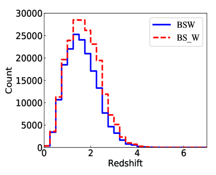
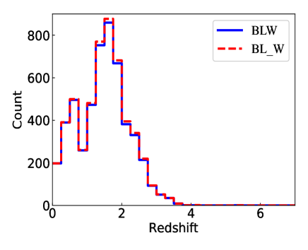
Figure 1: Left panel: the distribution of spectroscopic redshifts for known samples BSW (blue line) & BS_W (red dash line); right panel: the distribution of spectroscopic redshifts for known samples BLW (blue line) & BL_W (red dash line).

Then we split the sample BS_W into two datasets BSO and BSW according to whether both $W1mag$ and $W2mag$ are $NULL$ or not. When both $W1mag$ and $W2mag$ are $NULL$, this source belongs to the sample BSO, otherwise, it belongs to the sample BSW. Correspondingly, the sample BL_W is divided into two datasets BLO and BLW. In this paper, the samples BS_W and BSW are used as training set and test set, BL_W and BLW are used as external test set.

3 Method

3.1 CatBoost

Gradient Boosted Decision Trees (GBDT, Friedman et al., 2001) are a powerful tool for classification and regression tasks. CatBoost is developed by Yandex researchers and engineers (Liudmila et al.,, 2018), and a high-performance open source algorithm. It is a member of the family of GBDT machine learning ensemble techniques, which applies boosting method to build strong classifiers by means of learning multiple weak classifiers or regressors. It uses Oblivious Decision Trees (ODT) to build decision trees, which are full binary trees, furthermore, all non-leaf nodes of ODT will have the same splitting criteria. This design is helpful to speed up the score and avoid overfitting. It supports categorical features and text features in data without additional preprocessing, and uses the ordered target statistics method for encoding new features. Besides, it is easy to get good result with the default set of model parameters. Thus, a lot of time for tuning its model parameters will be saved. It also has fast and scalable GPU version fit for handling big data. Compared to GBDT, it has two innovations: ordered target statistics and ordered boosting.

3.2 XGBoost

XGBoost (Chen & Guestrin,, 2016) is an excellent ensemble learning algorithm. Compared with other ensemble models, it can improve the model’s robustness by introducing regular terms and column sampling; and when each tree selects the split point, a parallelization strategy will be adopted to improve the model’s running speed. Besides, XGBoost can overcome the limitations of computational speed and accuracy to a certain extent, require less training and prediction time, and support various objective functions, when performing classification and regression tasks.

3.3 Random Forest

Random Forest (RF, Breiman, 2001) is based on bagging models built using the decision tree method. RF uses bootstrap resampling technology to randomly select $K$ subsamples from the original training sample with replacement to generate a new training sample set, and build $K$ classification trees to form a random forest. Each tree in the forest has the same distribution, and the classification error depends on the classification ability of each tree and the correlation between them. Feature selection uses a random method to split each node, and then compares the errors generated in different situations. Therefore RF uses the average to improve the predictive accuracy and control over-fitting. In the scikit-learn implementation of RF combines classifiers by averaging their probabilistic prediction, instead of letting each classifier vote for a single class.

XGBoost and Random Forest methods have wide applications in astronomy, such as classification of unknown source (Mirabal et al.,, 2016), quasar candidate selection (Jin et al.,, 2019), photometric redshift estimation (Zhang et al.,, 2019) etc. CatBoost has various applications in different fields, such as finance, investment, petroleum and medicine. In this paper, we use XGBoost, CatBoost and Random Forest as supervised learning algorithms to build regressors for photometric redshift estimation of different quasar samples with different features. We also compare the performance of these three algorithms when classifying quasar sample into low- and high-redshift subsamples. CatBoost, XGboost and Random Forest python packages are provided by scikit-learn (Pedregosa et al.,, 2011) and all computing runs in the cloud computing environment of National Astronomical Data Centre (NADC) (Li et al.,, 2017).

4 Photometric redshift estimation

4.1 Regression Metrics

The performance evaluation of different algorithms about photometric redshift estimation depends on different metrics, such as the residual between the spectroscopic and photometric redshifts, $\Delta\rm z=\rm z_{\rm spec}-\rm z_{\rm photo}$, the mean absolute error (${\rm MAE}$) and the mean squared error (${\rm MSE}$). They are defined as follows:

$$MAE=\frac{1}{n}\sum_{i=0}^{n-1}|z_{i}-\widehat{z}_{i}|\\$$ (1)

$$MSE=\frac{1}{n}\sum_{i=0}^{n-1}(z_{i}-\widehat{z}_{i})^{2}\\$$ (2)

where $z_{i}$ is the true redshift, $\widehat{z_{i}}$ is the predicted redshift value and $n$ is the sample size.

The fraction of test sample that satisfies $|\rm\Delta{z}|<e$ is usually used to evaluate the redshift estimation, where $e$ is a given residual threshold (Schindler et al. 2017 and references therein). In reality, the redshift normalized residual ($\rm\Delta{z(norm)}$) is often adopted, and we use $e=0.3$.

$$\rm{{\Delta}z(norm)}=\frac{z_{\rm spec}-z_{\rm phot}}{1+z_{\rm spec}}\\$$ (3)

$$\rm{\delta_{0.3}}=\frac{\rm N_{\left|{\Delta}z(norm)\right|<0.3}}{\rm N_{total}}$$ (4)

Then, we use five additional metrics defined below as a reference for performance evaluation of different machine learning methods: $\mathrm{R}^{2}$, bias (the average separation between prediction and true values), the standard deviation between the photometric redshifts and the spectroscopic redshifts, the normalized median absolute deviation ($\sigma_{\mathrm{NMAD}}$) and the outlier fraction (O) (Ben et al.,, 2021; Curran et al.,, 2021).

$$\mathrm{R^{2}}=1-\frac{\sum_{i=1}^{n}|(z_{i}-\widehat{z}_{i})^{2}}{\sum_{i=1}^{n}(z_{i}-\overline{z})^{2}}\\$$ (5)

$$\mathrm{Bias}=<z_{\rm spec}-z_{\rm phot}>\\$$ (6)

$$\sigma_{{\Delta}\rm z}=\sqrt{\frac{1}{n}\sum_{i=0}^{n-1}(\rm{\Delta}z)^{2}}\\$$ (7)

$$\sigma_{\rm NMAD}=1.48\times\rm{median}\left|\frac{z_{\rm spec}-z_{\rm phot}}{1+z_{\rm spec}}\right|\\$$ (8)

$$Outlier\,\,fraction\,\,(O)=\frac{\rm N_{\left|{\Delta}z(norm)\right|>0.15}}{\rm N_{total}}$$ (9)

4.2 Feature selection

When handling high dimensional data, feature selection is the key factor influencing the performance of a machine learning algorithm. Feature selection not only reduces the dimension of data and rules out unimportant features, but also contributes to improve the accuracy of an algorithm. During data preprocessing, we need to obtain optimal features firstly, and adopt two steps for feature selection.

According to the parameters listed in Table 1, we define optical and infrared features. All optical features include $KronMag-PSFMag$ of g,r,z (namely ${\Delta}g$, ${\Delta}r$, ${\Delta}z$, respectively), $g$, $r$, $z$, $g-r$, $r-z$, $g-z$, and all infrared features are $W1$, $W2$, $g-W1$, $r-W1$, $z-W1$, $g-W2$, $r-W2$, $z-W2$, $W1-W2$. For the samples BSW and BS_W, they have all optical and infrared features. The difference between the samples BSW and BS_W is that the sample BS_W includes the samples BSW and BSO. Each source in the sample BSW contains both optical and infrared information while the sample BSO only includes optical information. The difference between the samples BLW and BL_W is same. The quasars of BSW and BS_W are from SDSS DR16Q, and the quasars of BLW and BL_W are from LAMOST DR5. As for the samples BSO and BLO, only the features from optical band are used. The sources in the samples BS_W and BL_W have no match sources in ALLWISE and no infrared features, so the features of these sources related to infrared band are missing. In other words, the samples BS_W and BL_W contain missing values. We set all missing values to 0 when using Random Forest. XGBoost and CatBoost support missing values.

Firstly, all features of training samples are evaluated by Random Forest, XGBoost and CatBoost methods, which can give the importance score of each feature. The importance type ($importance\_type$) is $total\_gain$. We sort these features by the importance score. The feature importance for different samples by different methods is shown in Figure 2. Figure 2 indicates that the feature importance is closely related to samples and algorithms. Furthermore, from the feature importance rank, it is seen that the infrared information is very important to the redshift estimation of quasars.

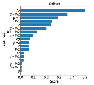
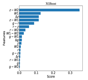
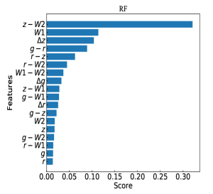
(a) For the sample BSW with optical and infrared features

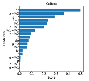
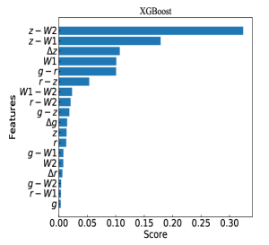
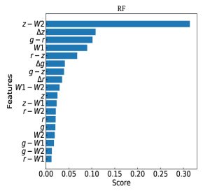
(b) For the sample BS_W with optical and infrared features

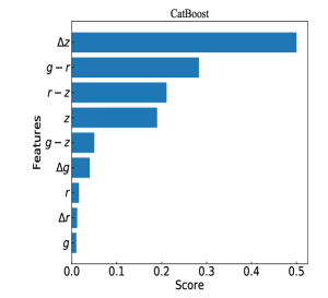
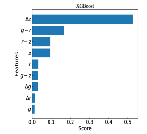
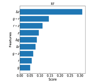
(c) For the sample BS_W only with optical features

Figure 2: The feature importance for different samples by CatBoost, XGBoost and Random Forest.

Secondly, when a method is adopted, according to the above rank of features, we select the top four features as initial input pattern to train a model, then add one feature in turn to the input pattern for training and record all performance. $MSE$ with different input features for different methods is described in Figure 3. For simplicity, the best input pattern is adopted when $MSE$ achieves the minimum. As shown in the left panel of Figure 3, for the sample BSW, the best input pattern is $z-W2$, $W1$, ${\Delta}z$, $z-W1$, $g-r$, $r-z$, $r-W2$, $W1-W2$, $g-W1$, ${\Delta}g$, $z$ (11 features) by XGBoost; the best input pattern is ${\Delta}z$, $z-W2$, $g-r$, $W1$, $r-z$, $z-W1$, $W1-W2$, $r-W2$, ${\Delta}g$, $g-z$, $z$, $W2$, ${\Delta}r$ (13 features) by CatBoost, and the best input pattern is $z-W2$, $W1$, ${\Delta}z$, $g-r$, $r-z$, $r-W2$, $W1-W2$, ${\Delta}g$, $z-W1$, $g-W1$, ${\Delta}r$, $g-z$, $W2$, $z$, $g-W2$ (15 features) by Random Forest. As plotted in the middle panel of Figure 3, for the sample BS_W, the optimal input pattern of XGBoost is $z-W2$, $z-W1$, ${\Delta}z$, $W1$, $g-r$, $r-z$, $W1-W2$, $r-W2$, $g-z$, ${\Delta}g$, $z$, $r$, $g-W1$, $W2$, ${\Delta}r$, $g-W2$ (16 features); the optimal input pattern of CatBoost is ${\Delta}z$, $z-W2$, $g-r$, $r-z$, $W1$, $z-W1$, $W1-W2$, $r-W2$, $z$, ${\Delta}g$, $g-z$, $W2$, ${\Delta}r$, $r$, $g-W2$ (15 features), and the optimal input pattern of Random Forest is $z-W2$, ${\Delta}z$, $g-r$, $W1$, $r-z$, ${\Delta}g$, $g-z$, ${\Delta}r$, $W1-W2$, $z$, $z-W1$, $r-W2$ (12 features). As indicated in the right panel of Figure 3, for the sample BS_W only with optical features, the optimal input patterns of the three methods keep all optical features (9 features) and retain their order. With the best input patterns for different samples by the three methods, we adopt the default hyper parameters of models and 5-fold cross validation to get the average values of $MSE$, $MAE$, bias, $\sigma_{\rm NMAD}$, $\sigma_{{\Delta}\rm z}$, $R^{2}$, ${\delta}_{0.3}$, $Outlier\,\,fraction\,\,(O)$ and running $time$, which are shown in Table 2. Comparing all metrics in Table 2, CatBoost achieves better performance than XGBoost and Random Forest for most metrics. In general, the better performance with optical and infrared features is archived than only with optical features. Table 2 further confirms this fact.

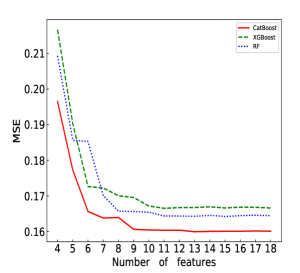
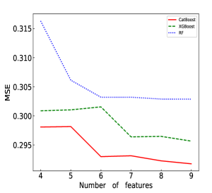
Figure 3: The performance of different methods with different input patterns for different samples. Left panel: for the sample BSW with optical and infrared information; middle panel: for the sample BS_W with optical and infrared information; right panel: for the sample BS_W only with optical information.

Table 2: The performance of photometric redshift estimation with optimal input features for each method with default model parameters

Sample	Input pattern	Method	MSE	MAE	$\mathrm{Bias}$	${\sigma}_{\rm NMAD}$	${\sigma}_{{\Delta}\rm z}$	$R^{2}$	${\delta}_{0.3}$(%)	$O$(%)	Time(s)
BSW	Pattern I	XGBoost	0.1666	0.2765	4.0 $\times 10^{-5}$	0.1070	0.4082	0.6493	93.39	22.04	3
BSW	Pattern II	CatBoost	0.1600	0.2702	6.0 $\times 10^{-5}$	0.1036	0.4000	0.6632	93.61	21.32	10
BSW	Pattern III	RF	0.1645	0.2700	2.2 $\times 10^{-3}$	0.1008	0.4056	0.6537	93.35	21.01	442
BS_W	Pattern IV	XGBoost	0.1925	0.3064	-7.6$\times 10^{-6}$	0.1171	0.4387	0.6071	92.37	25.22	6
BS_W	Pattern V	CatBoost	0.1867	0.3012	-4.8$\times 10^{-6}$	0.1146	0.4321	0.6189	92.56	24.48	12
BS_W	Pattern VI	RF	0.1924	0.3009	-2.0$\times 10^{-5}$	0.1107	0.4387	0.6074	92.32	24.03	447
BS_W	Pattern VII	XGBoost	0.2959	0.4009	-1.0 $\times 10^{-4}$	0.1657	0.5439	0.4008	87.27	37.40	4
BS_W	Pattern VII	CatBoost	0.2917	0.3988	-9.0 $\times 10^{-5}$	0.1651	0.5403	0.4087	87.39	37.74	12
BS_W	Pattern VII	RF	0.3032	0.4045	8.7 $\times 10^{-3}$	0.1648	0.5507	0.3858	86.52	37.93	200
a Pattern I represents $z-W2$, $W1$, ${\Delta}z$, $z-W1$, $g-r$, $r-z$, $r-W2$, $W1-W2$, $g-W1$, ${\Delta}g$, $z$ (11 features).
b Pattern II represents ${\Delta}z$, $z-W2$, $g-r$, $W1$, $r-z$, $z-W1$, $W1-W2$, $r-W2$, ${\Delta}g$, $g-z$, $z$, $W2$, ${\Delta}r$ (13 features).
c Pattern III represents $z-W2$, $W1$, ${\Delta}z$, $g-r$, $r-z$, $r-W2$, $W1-W2$, ${\Delta}g$, $z-W1$, $g-W1$, ${\Delta}r$, $g-z$, $W2$, $z$, $g-W2$ (15 features).
d Pattern IV represents $z-W2$, $z-W1$, ${\Delta}z$, $W1$, $g-r$, $r-z$, $W1-W2$, $r-W2$, $g-z$, ${\Delta}g$, $z$, $r$, $g-W1$, $W2$, ${\Delta}r$, $g-W2$ (16 features).
e Pattern V represents ${\Delta}z$, $z-W2$, $g-r$, $r-z$, $W1$, $z-W1$, $W1-W2$, $r-W2$, $z$, ${\Delta}g$, $g-z$, $W2$, ${\Delta}r$, $r$, $g-W2$ (15 features).
f Pattern VI represents $z-W2$, ${\Delta}z$, $g-r$, $W1$, $r-z$, ${\Delta}g$, $g-z$, ${\Delta}r$, $W1-W2$, $z$, $z-W1$, $r-W2$ (12 features).
g Pattern VII represents ${\Delta}z$, ${\Delta}g$, ${\Delta}r$, $g-r$, $g-z$, $r-z$, $g$, $r$, $z$ (9 features).
h Pattern I, II, III, IV, V, VI, VII represents the same meaning in the following of this paper.

4.3 Model parameter optimization

Since the optimal input patterns have been set, the next task is to determine the hyper parameters of models. Model parameter optimization is a very complex task. In order to reduce computing scale, we only choose some main hyper parameters for each method. For XGBoost, the important model parameters contain the maximum depth of individual trees (max_depth) and the number of weak estimators (n_estimators); for CatBoost, the key model parameters are the maximum depth of individual tree (depth) and the maximum number of trees (iterations); for Random Forest, the main model parameters are the maximum depth of individual trees (max_depth) and the number of trees in the forest (n_estimators). We adopt the grid search method to get the optimal model parameters and 5-fold cross validation to get the average values of $MSE$, $MAE$, $Bias$, ${\sigma}_{\rm NMAD}$, ${\sigma}_{{\Delta}z}$, $R^{2}$, ${\delta}_{0.3}$, $O$ and running $time$. The optimal model parameters and performance are listed in Table 3. As described in Table 3, the best performance is obtained on the sample BSW for these three methods, $MSE$, $MAE$, $Bias$, ${\sigma}_{\rm NMAD}$, ${\sigma}_{{\Delta}z}$, $R^{2}$, ${\delta}_{0.3}$ and $O$ respectively amount to 0.1576, 0.2649, -0.0006, 0.0999, 0.3971, 0.6680, 93.78, 20.45 for CatBoost; 0.1617, 0.2669, -0.0009, 0.1001, 0.4022, 0.6595, 93.61, 20.58 for XGBoost; 0.1626, 0.2686, 0.001, 0.1007, 0.4032, 0.6578, 93.50, 20.83 for Random Forest, respectively. Table 3 also shows that for the samples BS_W, the performance with optical and infrared information are better than that only with optical information for any method. Comparison of the performance of XGBoost, CatBoost and Random forest in Table 3, CatBoost shows its superiority.

Then, with optimal model parameters and 80:20 training-test split, we train again for the samples BSW and BS_W. The scatter figure and $\Delta{\rm z(norm)}$ distribution of estimated photometric redshifts and spectroscopic redshifts are shown in Figure 4. Figure 4 further proves that CatBoost outperforms XGBoost and Random Forest.

Table 3: The performance of photometric redshift estimation with the best features and optimal model parameters

Sample	Input pattern	Method	Model parameter	MSE	MAE	$\mathrm{Bias}$	${\sigma}_{\rm NMAD}$	${\sigma}_{{\Delta}\rm z}$	$R^{2}$	${\delta}_{0.3}$(%)	$O$(%)	Time(s)
BSW	Pattern I	XGBoost	max_depth=11	0.1617	0.2669	-0.0009	0.1001	0.4022	0.6595	93.61	20.58	110
			n_estimators=1000
BSW	Pattern II	CatBoost	depth=12	0.1576	0.2649	-0.0006	0.0999	0.3971	0.6680	93.78	20.45	421
			iterations=4000
BSW	Pattern III	RF	max_depth=15	0.1626	0.2686	0.0001	0.1007	0.4032	0.6578	93.50	20.83	1336
			n_estimators=500
BS_W	Pattern IV	XGBoost	max_depth=10	0.1865	0.2969	0.0001	0.1106	0.4318	0.6195	92.62	23.72	325
			n_estimators=1200
BS_W	Pattern V	CatBoost	depth=12	0.1848	0.2960	0.0001	0.1105	0.4299	0.6228	92.69	23.55	468
			iterations=4000
BS_W	Pattern VI	RF	max_depth=15	0.1893	0.2990	0.0009	0.1111	0.4351	0.6136	92.44	23.82	1431
			n_estimators=500
BS_W	Pattern VII	XGBoost	max_depth=10	0.2930	0.3967	-0.0001	0.1626	0.5413	0.4066	87.43	37.17	110
			n_estimators=1000
BS_W	Pattern VII	CatBoost	depth=12	0.2906	0.3970	-0.0001	0.1637	0.5393	0.4110	87.47	37.38	254
			iterations=2000
BS_W	Pattern VII	RF	max_depth=15	0.2944	0.3975	0.0003	0.1623	0.5425	0.4038	87.36	37.07	1124
			n_estimators=500

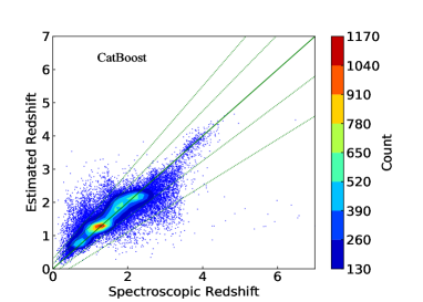
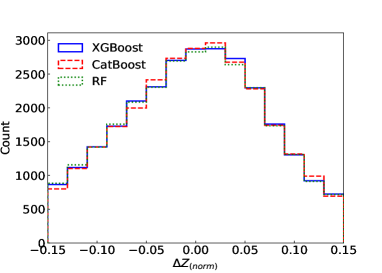
(a) For the sample BSW

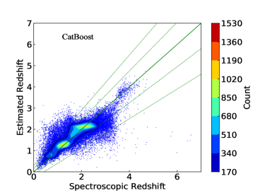
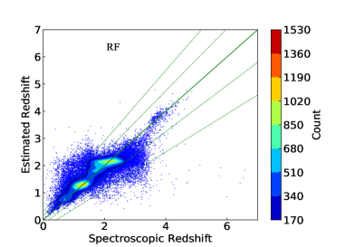
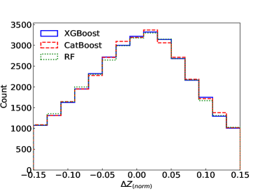
(b) For the sample BS_W

Figure 4: The first three plots in (a) and (b) show the performance of photometric redshift estimation with CatBoost, XGBoost and RF, respectively. The green line represents $\Delta\rm z=0$; the green dotted lines represent $\Delta\rm z(norm)=\pm 0.15,\pm 0.3$, separately. The last plots in (a) and (b) show the distribution of $\Delta\rm z(norm)$.

Finally, we use the three optimal models to train regressors with the total samples, and apply the total samples and external samples as test samples separately to validate the regressors, the validation performance is shown in Table 4. Table 4 tells that when the regressors created with optical and infrared information is applied, the performance of CatBoost with Pattern II is $MSE=0.1059$, $MAE=0.2223$, $Bias=-1.6\times 10^{-5}$, ${\sigma}_{\rm NMAD}=0.0872$, ${\sigma}_{{\Delta}z}=0.3254$, $R^{2}=0.7780$, ${\delta}_{0.3}=96.01\%$ and $O=15.79\%$ for the test sample BSW; the performance of CatBoost with Pattern II is with $MSE=0.1239$, $MAE=0.2134$, $Bias=0.0265$, ${\sigma}_{\rm NMAD}=0.0797$, ${\sigma}_{{\Delta}z}=0.3520$, $R^{2}=0.7585$, ${\delta}_{0.3}=94.50\%$ and $O=15.11\%$ for the test sample BLW. For the test sample BL_W or BSO, the regressor with Pattern V is better than that with Pattern VII, which suggests that the regressor with Pattern V had better be adopted although the sources to be predicted only contain optical information. For the test sample BLW or BSW, the regressor with Pattern II is superior to that with Pattern V. Therefore the sources with optical and infrared information had better be estimated by the regressor with Pattern II. Table 4 further shows that the CatBoost regressors are effective to predict photometric redshifts of quasars.

Table 4: The performance of CatBoost for photometric redshift estimation.

Training Sample	Input pattern	Test Sample	MSE	MAE	$\mathrm{Bias}$	${\sigma}_{\rm NMAD}$	${\sigma}_{{\Delta}\rm z}$	$R^{2}$	${\delta}_{0.3}$(%)	$O$(%)
BSW	Pattern II	BSW	0.1059	0.2223	-1.6 $\times 10^{-5}$	0.0872	0.3254	0.7780	96.01	15.79
BSW	Pattern II	BLW	0.1239	0.2134	0.0265	0.0797	0.3520	0.7585	94.50	15.11
BS_W	Pattern V	BSW	0.1115	0.2279	-4.0 $\times 10^{-5}$	0.0889	0.3340	0.7661	95.77	16.42
BS_W	Pattern V	BS_W	0.1365	0.2578	-7.0 $\times 10^{-6}$	0.0981	0.3695	0.7239	94.84	19.42
BS_W	Pattern V	BLW	0.1265	0.2167	0.0268	0.0808	0.3557	0.7534	94.48	15.61
BS_W	Pattern V	BL_W	0.1277	0.2188	0.0296	0.0817	0.3574	0.7502	94.41	15.87
BS_W	Pattern V	BSO	0.2490	0.3929	1.2 $\times 10^{-4}$	0.1550	0.4991	0.3884	90.64	32.93
BS_W	Pattern VII	BSO	0.3267	0.4363	-0.1853	0.1672	0.5719	0.1970	90.98	36.97
BS_W	Pattern VII	BL_W	0.2596	0.3681	0.1223	0.1639	0.5095	0.4925	85.82	37.61

5 Two-step model

In the whole quasar samples, the number of high redshift quasars (redshift $\geq 3.5$) is relatively small compared to that of low redshift quasars (redshift $<3.5$). In the sample BS_W, there are only 2238 high redshift quasars among the 213 359 quasars, while in the sample BSW, there are only 1798 high redshift quasars among 174 645 quasars. The sample BS_W is divided into high redshift subsample BS_W_H and low redshift subsample BS_W_L, similarly the sample BSW is split into BSW_H and BSW_L. Table 5 shows the performance of photometric redshift estimation for high redshift and low redshift subsamples based on the best CatBoost regressors in Table 4. As described in Table 5, the performance on the high redshift subsamples is much worse than that on the low redshift subsamples for the sample BS_W or BSW. Meanwhile, Figure 4 indicates that many high redshift quasars have been predicted as low redshift quasars. For the sample BS_W, there are only 1765 quasars which are correctly predicted as high redshift quasars among 2238 high redshift quasars, taking up about 78 per cent, while for the sample BSW, 1492 quasars are correctly predicted as high redshift quasars among 1798, occupying about 83 per cent. It is obvious that the regressor fit for low redshift quasars is not fit for high redshift quasars. Thus, we propose a two-step model to improve the performance of redshift estimation for quasars, especially for high redshift quasars.

Table 5: The performance of photometric redshift estimation for high and low subsamples with the best CatBoost regressors in Table 4.

Training Sample	Pattern	Test Sample	MSE	MAE	$\mathrm{Bias}$	${\sigma}_{\rm NMAD}$	${\sigma}_{{\Delta}\rm z}$	$R^{2}$	${\delta}_{0.3}$(%)	$O$(%)
BS_W	Pattern V	BS_W_H	0.4079	0.2799	-0.1943	0.0359	0.6387	-1.4640	96.15	8.04
BS_W	Pattern V	BS_W_L	0.1336	0.2575	0.0021	0.0989	0.3655	0.7019	94.83	19.34
BSW	Pattern II	BSW_H	0.4074	0.2575	-0.1741	0.0318	0.6383	-1.1900	96.27	6.7
BSW	Pattern II	BSW_L	0.1027	0.2219	0.0018	0.0879	0.3205	0.7591	96.00	15.89

5.1 The first step of the two-step model

In order to improve the performance of photometric redshift estimation of quasars, we put forward a new scheme of first classification and second regression (i.e. two-step model) for photometric redshift estimation. The first step of two-step model is to construct a classifier to discriminate the whole quasars into low and high redshift subsamples. Based on the samples BSW and BS_W, we add a column “label”, which is 1 if redshift $\geq$ 3.5, otherwise, set to 0. We adopt four standard metrics (Accuracy, Precision, Recall, and F1_score) to evaluate the performance of one classifier. Accuracy (Accu.) is the ratio of the number of the correctly classified samples to the total number of the samples.

$$\mathrm{Accuracy}=\frac{TP+TN}{TP+TN+FP+FN}$$ (10)

Here TP and TN are correctly classified by the classifier. FP shows the negative sample classified as positive. FN represents the positive sample classified as negative.

Precision (Prec.) is the ratio of the true positive (negative) sample in all the samples that are classified as positive (negative). Recall (Rec.) is the ratio of correctly classified positive (negative) samples in all the true positive (negative) samples.

$$\mathrm{Precison}=\frac{TP}{TP+FP},\mathrm{Recall}=\frac{TP}{TP+FN}$$ (11)

F1_score (F1) is a weighted average of Precision and Recall.

$$\mathrm{F1\_score}=\frac{2\times(\mathrm{Prec}.\times\mathrm{Rec.})}{\mathrm{Prec.}+\mathrm{Rec.}}$$ (12)

Then we use CatBoost, XGBoost and Random Forest to construct binary classifiers, the optimal performance and hyper parameters of the three classifiers by five-fold validation are shown in Table 6. Table 6 shows that CatBoost is superior to XGBoost and Random Forest when separating the sample BSW or BS_W into low and high redshift subsamples considering Accuracy and F1_score. Moreover Recall (completeness) of CatBoost achieves the best for high redshift quasars. In order to find more high redshift quasars, we should keep high completeness at high redshift in the first step of two-step model.

Table 6: The performance of different classifiers for high and low redshift subsamples.

					High redshift			Low redshift
Sample	Input Pattern	Method	Parameter	Accu.(%)	Prec.(%)	Rec.(%)	F1(%)	Prec.(%)	Rec.(%)	F1(%)	Time(s)
BSW	Pattern I	XGBoost	max_depth=6	99.78	92.48	86.10	89.18	99.86	99.92	99.89	124
			n_estimators=200
BSW	Pattern II	CatBoost	depth=6	99.79	92.33	87.04	89.60	99.87	99.93	99.90	19
			iterations=1000
BSW	Pattern III	RF	max_depth=14	99.78	93.91	84.54	88.98	99.84	99.94	99.89	190
			n_estimators=500
BS_W	Pattern IV	XGBoost	max_depth=6	99.77	92.30	85.12	88.56	99.84	99.92	99.87	46
			n_estimators=100
BS_W	Pattern V	CatBoost	depth=12	99.78	92.87	85.21	88.88	99.84	99.93	99.88	130
			iterations=1000
BS_W	Pattern VI	RF	max_depth=13	99.77	93.88	82.89	88.04	99.82	99.94	99.87	72
			n_estimators=100

In order to further test the performance of CatBoost, XGBoost and Random Forest classifiers, we use the whole quasar samples from SDSS as training and test samples. The self-validation classification performance of the three classifiers is shown in Table 7. It can be seen from Table 7 that the CatBoost classifier based on the sample BS_W has better performance than that based on the sample BSW when the sample BSW is taken as test sample. The better performance is that Accuracy reaches 99.99 per cent, F1 is 99.96 per cent for the high redshift subsample, and F1 is 99.99 per cent for the low redshift subsample. Therefore the CatBoost classifier based on the sample BS_W is more suitable for the sample BSW. In other words, the CatBoost classifier created on the training sample BS_W had better be adopted for the sources with optical information or those with optical and infrared information. When the BSW sample is taken as training and test samples, XGBoost achieves the best performance while CatBoost and Random Forest obtain the same performance (all metrics above 96.27 per cent). In other two situations, CatBoost is superior to XGBoost and Random Forest, moreover the running time of CatBoost is the fastest. Therefore CatBoost is adopted as the core algorithm of classification in the first step of the whole scheme.

Table 7: The performance of different classifiers with different training and test samples.

					High redshift			Low redshift
Training Sample	Method	Input  pattern	Test Sample	Accu.(%)	Prec.(%)	Rec.(%)	F1(%)	Prec.(%)	Rec.(%)	F1(%)	Time(s)
BSW	CatBoost	Pattern II	BSW	99.96	100	96.27	98.10	99.96	100	99.98	0.25
BS_W	CatBoost	Pattern V	BSW	99.99	100	99.94	99.97	99.99	100	100	0.27
BS_W	CatBoost	Pattern V	BS_W	99.99	100	99.91	99.95	99.99	100	100	0.36
BSW	XGBoost	Pattern I	BSW	100	100	100	100	100	100	100	2
BS_W	XGBoost	Pattern IV	BSW	99.97	99.60	98.00	98.79	99.98	99.99	99.99	1.5
BS_W	XGBoost	Pattern IV	BS_W	99.97	99.68	97.90	98.78	99.98	99.99	99.99	2
BSW	RF	Pattern III	BSW	99.96	100	96.27	98.10	99.96	100	99.98	11
BS_W	RF	Pattern VI	BSW	99.93	99.53	94.16	96.77	99.94	99.99	99.96	3
BS_W	RF	Pattern VI	BS_W	99.92	99.33	93.07	96.10	99.93	99.99	99.96	3

5.2 The second step of the two-step model

High and low redshift subsamples of BSW and BS_W are trained to construct new regressors by CatBoost, XGBoost and Random Forest, respectively. The optimal model parameters and performance of all subsamples for these three methods are shown in Table 8. As shown in Table 8, the performance of both low and high redshift subsamples has been significantly improved, especially for high redshift quasars. Taking the evaluation metrics of regression into account except Bias, ${\sigma}_{\mathrm{NMAD}}$ and $O$ in Table 8, CatBoost outperforms XGBoost and Random Forest for any sample. Only given ${\sigma}_{\mathrm{NMAD}}$, CatBoost obtains the best performance for the samples BSW_L and BS_W_L. Only considering $O$, CatBoost shows its superiority for the samples BSW_H, BSW_L and BS_W_L. As a result, CatBoost is taken as the core regression algorithm for the two-step model.

Table 8: The performance of photometric redshift estimation on different subsamples with different methods.

Sample	Input pattern	Method	Model parameter	MSE	MAE	$\mathrm{Bias}$	${\sigma}_{\mathrm{NMAD}}$	${\sigma}_{\mathrm{{\Delta}\rm z}}$	$R^{2}$	${\delta}_{0.3}$(%)	$O$(%)	Time(s)
BSW_H	Pattern I	XGBoost	max_depth=6	0.0989	0.1515	-0.0254	0.0253	0.3144	0.4777	99.11	2.56	2
			n_estimators=500
BSW_H	Pattern II	CatBoost	depth=7	0.0756	0.1439	-0.0055	0.0256	0.2750	0.5910	99.72	2.17	5
			iterations=3000
BSW_H	Pattern III	RF	max_depth=11	0.0781	0.1442	0.0035	0.0253	0.2796	0.5804	99.55	2.4	14
			n_estimators=1000
BSW_L	Pattern I	XGBoost	max_depth=10	0.1526	0.2646	-0.0017	0.1012	0.3907	0.6408	93.77	20.64	32
			n_estimators=700
BSW_L	Pattern II	CatBoost	depth=13	0.1497	0.2624	-0.0005	0.1002	0.3870	0.6475	93.85	20.37	285
			iterations=3000
BSW_L	Pattern III	RF	max_depth=15	0.1536	0.2656	0.0010	0.1012	0.3919	0.6386	93.67	20.68	1300
			n_estimators=500
BS_W_H	Pattern IV	XGBoost	max_depth=5	0.0800	0.1429	-0.0068	0.0250	0.2828	0.5119	99.51	2.24	3
			n_estimators=1000
BS_W_H	Pattern V	CatBoost	depth=6	0.0759	0.1404	-0.0081	0.0248	0.2756	0.5407	99.64	2.32	5
			iterations=2000
BS_W_H	Pattern VI	RF	max_depth=11	0.0769	0.1405	-0.0007	0.0242	0.2773	0.5285	99.51	2.59	5
			n_estimators=300
BS_W_L	Pattern IV	XGBoost	max_depth=10	0.1791	0.2947	-0.0002	0.1109	0.4233	0.5967	92.72	23.66	370
			n_estimators=1000
BS_W_L	Pattern V	CatBoost	depth=13	0.1775	0.2934	-0.0001	0.1105	0.4213	0.6005	92.80	23.52	450
			iterations=3000
BS_W_L	Pattern VI	RF	max_depth=15	0.1812	0.2963	0.0006	0.1115	0.4257	0.5919	92.60	23.76	2811
			n_estimators=1000

5.3 Comparison of two-step model with one-step model

For the two-step model, its first step is to classify the sample into low and high redshift subsamples; its second step is to create CatBoost regressors for low and high redshift subsamples respectively. According to the above experiments, CatBoost is regarded as the core algorithms for both classification and regression. The CatBoost classifier is trained on the BS_W sample no matter whether the sources own infrared information, while the CatBoost regressors for low and high redshift subsamples are trained on the samples BS_W_L and BS_W_H for sources only with optical information and trained on the samples BSW_L and BSW_H with optical and infrared information. We use the samples BSW, BS_W, BLW and BL_W to test models. Table 4 gives the performance of photometric redshift estimation by one-step model. In order to compare the performance of photometric redshift estimation between one-step model and two-step model, the test results of the two models with different test samples are indicated in Table 9. Taking the samples BSW and BS_W for example, the comparison of predicted photometric redshifts with spectroscopic redshifts is described in Figures 5 and the ${\Delta}{\mathrm{z}}$ distribution is indicated in Figure 6. In Figure 5, the left ones are the results of two-step model, the right ones are those of one-step model. As shown in Figure 5, the number of outliers for two-step model is less than that for one-step model, especially in the range of high redshift. From the evaluation metrics of regression in Table 9 and outliers in Figure 5, it is obvious that the performance of two-step model is better than that of one-step model. Figure 6 further proves this result.

Table 9: Comparison of the performance of photometric redshift estimation by two-step model with that by one-step model.

Test Sample	MSE	MAE	$\mathrm{Bias}$	${\sigma}_{\mathrm{NMAD}}$	${\sigma}_{\mathrm{{\Delta}z}}$	$R^{2}$	${\delta}_{0.3}$(%)	$O$(%)	Time(s)
			two-step model
BSW	0.0970	0.2153	-0.00004	0.0854	0.3114	0.7967	96.32	15.13	25.0
BLW	0.1216	0.2103	0.0249	0.0784	0.3487	0.7630	94.86	14.81	2.0
BS_W	0.1266	0.2499	-0.00004	0.0955	0.3558	0.7440	96.32	18.67	35.0
BL_W	0.1251	0.2157	0.0280	0.0804	0.3537	0.7553	94.40	15.63	9.0
			one-step model
BSW	0.1059	0.2223	-0.00002	0.0872	0.3254	0.7780	96.01	15.80	0.80
BLW	0.1239	0.2134	0.0265	0.0797	0.3521	0.7585	94.50	15.11	0.03
BS_W	0.1365	0.2578	-0.000007	0.0981	0.3695	0.7239	94.84	19.42	1.00
BL_W	0.1277	0.2188	0.0296	0.0817	0.3574	0.7502	94.40	15.88	0.05

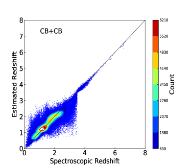
(a) For the sample BSW.

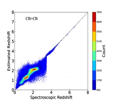
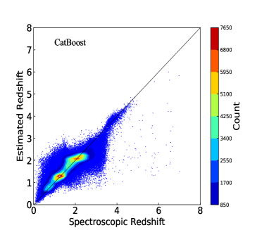
(b) For the sample BS_W.

Figure 5: Comparison of the photometric redshift with the spectroscopic redshift for the samples BSW and BS_W with two-step models (left panel) and one-step models (right panel), respectively.

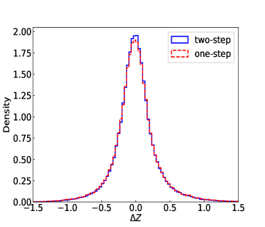
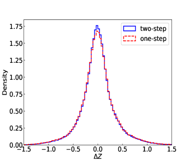
Figure 6: The ${\Delta}{\mathrm{z}}$ distribution for the samples BSW (left panel) and BS_W (right panel) with two-step models and one-step models during the range from -1.5 to 1.5, respectively.

5.4 Application

Based on the above experimental results for the known samples, we put forward a workflow of photometric redshift estimation as shown in Figure 7, which is applied to predict photometric redshifts of quasar candidates from BASS DR3. In Figure 7, the red rectangle boxes indicate data analysis and black parallelograms represent intermediate data or results. The workflow includes six regressors and one classifier. The detailed model information of this workflow is shown in Table 10.

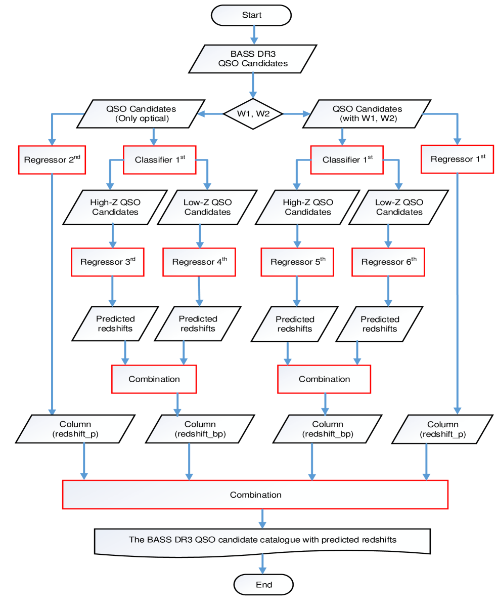
Figure 7: The photometric redshift estimation workflow.

Table 10: The models used in photometric redshift estimation workflow.

Scheme	Method	Input pattern		Redshift range	$W1$, $W2$
Regressor $1^{st}$	CatBoost	Pattern II		Full	Indispensable
Regressor $2^{nd}$	CatBoost	Pattern V		Full	Dispensable
Regressor $3^{rd}$	CatBoost	Pattern II		Redshift $\geq$ 3.5	Indispensable
Regressor $4^{th}$	CatBoost	Pattern II		Redshift $<$ 3.5	Indispensable
Regressor $5^{th}$	CatBoost	Pattern V		Redshift $\geq$ 3.5	Dispensable
Regressor $6^{th}$	CatBoost	Pattern V		Redshift $<$ 3.5	Dispensable
Classifier $1^{st}$	CatBoost	Pattern III		(High redshift and low redshift)	Dispensable

According to the work Li et al., (2021), the BASS DR3 Sources were identified as Stars, Galaxies and Quasars by XGBoost. We consider all possible quasar candidates, the total number of which is 26 200 778. We adopt the workflow to estimate their photometric redshifts.

In Figure 7, BASS-DR3 quasar candidates are firstly divided into two samples. One sample contains only optical features, and the other sample contains optical and infrared features. For the candidates with optical and infrared features, we get predicted redshifts $redshift\_p$ by Regressor ^1st, and these candidates are also classified into high redshift (high-Z) and low redshift (low-Z) subsamples. For the candidates classified as high-Z sources, we use Regressor ^3rd to estimate redshifts, while for candidates classified as low-Z sources, Regressor ^4th is used. Similarly, we obtain estimated redshifts of the candidates with only optical features. $redshift\_bp$ is predicted by two-step model while $redshift\_p$ is from one-step model. In the end, all predicted results are combined in a whole table. The link address is http://paperdata.china-vo.org/Li.Changhua/bass/bassdr3-quasar-z.hdf5. Table 11 lists 20 rows of predicted results, which is of great value for the further research on the characteristics and physics of these quasar candidates.

Table 11: The estimated redshifts of BASS DR3 quasar candidates, redshift$\_bp$ is predicted redshift by two-step model, redshift$\_p$ is predicted redshift by one-step model.

id	ra	dec	redshift$\_bp$	redshift$\_p$
95429001151	133.48449872099638	84.64760058245369	3.612	2.755
95375007162	146.34468863159154	84.19521072349899	3.756	2.967
95375009802	146.70683096395808	84.34011991887981	3.853	3.071
95376013790	156.8204830082884	84.55993969686726	3.820	3.462
95432000953	156.68410784655092	84.62164596197978	3.770	2.216
95433002683	162.41293319964882	84.75661154235415	3.831	3.252
95379009607	172.10642294951734	84.54070384254878	4.290	2.970
95435000350	172.16026329686127	84.59069887892409	3.584	2.644
95439001178	204.45978967988097	84.63147943935314	3.703	2.324
95440003112	208.24299714603515	84.74509303019737	3.835	2.349
95440003256	207.3572024876584	84.75161970723823	3.657	3.329
95441002154	214.02787846450985	84.7184000420548	3.643	2.777
95372005855	128.4637617956736	84.17660965013285	3.690	2.329
95372007632	127.96938333672199	84.25455113312614	3.818	3.120
95372008421	129.9774226081903	84.30134401378302	3.753	2.407
95373007697	136.73203714550777	84.23113544297041	3.875	2.745
95373009831	138.71782967532423	84.32491202628485	3.725	2.288
95374010575	143.50234604548734	84.37099267752663	3.858	3.136
95312008225	151.1039377338386	83.5936910539942	3.716	3.013
95312012685	150.5329880180199	83.78811573097289	3.861	1.869
95376009700	153.0999380695831	84.3246689896127	3.738	2.487

In the work Li et al., (2021), when applying both optical and infrared information with the same predicted results by binary and multiclass classifiers, the number of quasar candidates is 2 195 180, 1 500 099 ($P_{\rm Q}>0.75$), and 798 928 ($P_{\rm Q}>0.95$). In Figure 8, we show the number density distribution of quasar candidates as a function of photometric redshifts estimated by one- and two-step models. It is found from Figure 8 that there is some difference between one- and two-step models for the predicted redshifts of the quasar candidates. Table 12 lists the number of BASS DR3 quasar candidates with $P_{\rm Q}>0.95$ in different redshift ranges by the two models, which suggests that two-step model is more easy to find high redshift quasars than one-step model.

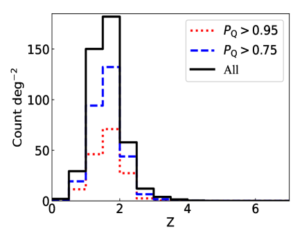
Figure 8: Left panel: the number density of quasar candidates as a function of photometric redshifts by two-step model; Right panel: the number density of quasar candidates as a function of photometric redshifts by one-step model (Regressor $1^{st}$). In both panels, the quasar candidates contain both optical and infrared information with the same predicted results by binary and multiclass classifiers for different probabilities ($P_{Q}>0.95$: red dotted line, $P_{Q}>0.75$: blue dotted dash line, all: black line).

Table 12: The number of BASS DR3 quasar candidates with $P_{\rm Q}>0.95$ in different redshift ranges by two models.

Model	redshift$<3.5$	$3.5\leq$redshift$<4.5$	$4.5\leq$redshift$<5.5$	redshift$\geq 5.5$
one-step	796078	2822	27	1
two-step	794990	3817	97	24

6 Conclusions

We present two schemes of machine-learning to predict photometric redshifts of quasars. We discuss the feature importance of different samples by XGBoost, CatBoost and Random forest. The optimal features and optimal model parameters of these three algorithms are chosen for different samples. Comparison of classification and regression of these three algorithms is performed. By contrast, CatBoost achieves the best performance among all classifiers and regressors for different samples considering effectiveness and efficiency. Moreover comparing the performance of two-step model with that of one-step model, two-step model is superior to one-step model. The two-step model is vital to select out high redshift quasar candidates. Therefore we put forward a photometric redshift workflow, in which CatBoost is taken as the core algorithm for classification and regression and two models are adopted. Then we utilize the workflow to predict photometric redshifts of all quasar candidates from BASS DR3. The predicted result will be of great help and reference for future research of quasars and can help LAMOST, DESI or other projects for follow up observation to find more high redshift quasars.

7 Acknowledgements

We are very grateful to the referee for his constructive suggestions and comments. This work is supported by National Natural Science Foundation of China (NSFC)(grant Nos. 11573019, 11803055, 11873066, 12133001, 11433005), the Joint Research Fund in Astronomy (U1531246, U1731125, U1731243, U1731109) under cooperative agreement between the NSFC and Chinese Academy of Sciences (CAS), the 13th Five-year Informatization Plan of Chinese Academy of Sciences (No. XXH13503-03-107) and the science research grants from the China Manned Space Project with NO. CMS-CSST-2021-A06. We would like to thank the National R&D Infrastructure and Facility Development Program of China, “Earth System Science Data Sharing Platform” and “Fundamental Science Data Sharing Platform” (DKA2017-12-02-07). Data resources are supported by Chinese Astronomical Data Center (NADC) and Chinese Virtual Observatory (China-VO). This work is supported by Astronomical Big Data Joint Research Center, co-founded by National Astronomical Observatories, Chinese Academy of Sciences and Alibaba Cloud. This research has made use of BASS DR3 catalogue. BASS is a collaborative program between the National Astronomical Observatories of the Chinese Academy of Science and Steward Observatory of the University of Arizona. It is a key project of the Telescope Access Program (TAP), which has been funded by the National Astronomical Observatories of China, the Chinese Academy of Sciences (the Strategic Priority Research Program. The Emergence of Cosmological Structures grant no. XDB09000000), and the Special Fund for Astronomy from the Ministry of Finance. BASS is also supported by the External Cooperation Program of the Chinese Academy of Sciences (grant No. 114A11KYSB20160057). The BASS data release is based on the Chinese Virtual Observatory (China-VO). The Guoshoujing Telescope (the Large Sky Area Multi-object Fiber Spectroscopic Telescope, LAMOST) is a National Major Scientific Project built by the Chinese Academy of Sciences. Funding for the project has been provided by the National Development and Reform Commission. LAMOST is operated and managed by the National Astronomical Observatories, Chinese Academy of Sciences.

We acknowledgment SDSS databases. Funding for the Sloan Digital Sky Survey IV has been provided by the Alfred P. Sloan Foundation, the U.S. Department of Energy Office of Science, and the Participating Institutions. SDSS-IV acknowledges support and resources from the Center for High-Performance Computing at the University of Utah. The SDSS web site is www.sdss.org. SDSS-IV is managed by the Astrophysical Research Consortium for the Participating Institutions of the SDSS Collaboration including the Brazilian Participation Group, the Carnegie Institution for Science, Carnegie Mellon University, the Chilean Participation Group, the French Participation Group, Harvard-Smithsonian Center for Astrophysics, Instituto de Astrofísica de Canarias, The Johns Hopkins University, Kavli Institute for the Physics and Mathematics of the Universe (IPMU) /University of Tokyo, Lawrence Berkeley National Laboratory, Leibniz Institut für Astrophysik Potsdam (AIP), Max-Planck-Institut für Astronomie (MPIA Heidelberg), Max-Planck-Institut für Astrophysik (MPA Garching), Max-Planck-Institut für Extraterrestrische Physik (MPE), National Astronomical Observatories of China, New Mexico State University, New York University, University of Notre Dame, Observatário Nacional / MCTI, The Ohio State University, Pennsylvania State University, Shanghai Astronomical Observatory, United Kingdom Participation Group, Universidad Nacional Autónoma de México, University of Arizona, University of Colorado Boulder, University of Oxford, University of Portsmouth, University of Utah, University of Virginia, University of Washington, University of Wisconsin, Vanderbilt University, and Yale University.

8 Data availability

The predicted photometric redshifts for BASS-DR3 quasar candidates are saved in a repository and can be obtained by a unique identifier, part of which is indicated in Table 11. It is put in paperdata at http://paperdata.china-vo.org, and can be available with http://paperdata.china-vo.org/Li.Changhua/bass/bassdr3-quasar-z.hdf5.

References

- Baum et al., (1957) Baum W. A. 1957, AJ. 62, 6
- Ball et al. (2007) Ball N. M., Brunner R. J., Myers A. D., Strand N. E., Alberts S. L., Tcheng D., Llor X., 2007, ApJ, 663(2), 774
- Ben et al., (2021) Ben Henghes, Connor Pettitt, Jeyan Thiyagalingam, Tony Hey, Ofer Lahav, 2021, MARAS, 505, 4847
- Blanton et al., (2017) Blanton M. R. et al., 2017, AJ, 154, 28
- Bonfield et al. (2010) Bonfield D. G., Sun Y., Davey N., Jarvis M. J., Abdalla F. B., Banerji M., Adams R. G., 2010, MNRAS, 405(2), 987
- Breiman, (2001) Breiman L. 2001, Machine Learning, 45, 5
- Brescia et al. (2013) Brescia M., Cavuoti S., D’Abrusco R., Longo G., Mercurio A., 2013, ApJ, 772(2), article id. 140, 12 pp
- Carliles et al. (2010) Carliles S., Budavri T., Heinis S., Priebe C., Szalay A. S., 2010, ApJ, 712(1), 511
- Carrasco & Brunner (2014) Carrasco K. M., Brunner, R. J., 2014, MNRAS, 438(4), 3409
- Cavuoti et al. (2012) Cavuoti S., Brescia M., Longo G., Mercurio A., 2012, A&A, 546, id.A13, 8 pp
- Cavuoti et al. (2017) Cavuoti S., Amaro V., Brescia M., Vellucci C., Tortora C., Longo G., 2017, MNRAS, 465(2), 1959
- Chen & Guestrin, (2016) Chen T., Guestrin C., 2016, Proceedings of the 22nd ACM SIGKDD International Conference on Knowledge Discovery and Data Mining. ACM
- Cui et al., (2012) Cui X.-Q., et al. 2012, RAA, 12, 1197
- Curran et al., (2021) Curran S. J., Moss J. P., Perrott Y. C., 2021, MNRAS, 503, 2639
- Firth, Lahav & Somerville (2003) Firth A. E., Lahav O., Somerville R. S., 2003, MNRAS, 339(4), 1195
- Friedman et al., (2001) Friedman J. H., 2001, Ann. Stat., 29, 1189
- Han et al., (2021) Han B., Qiao L.-N., Chen J.-L., Zhang X.-D., Zhang Y.-X., Zhao Y.-H., 2021, RAA, 219(1), 17
- Hoyle (2016) Hoyle B., 2016, Astronomy and Computing, 16, 34
- Jin et al., (2019) Jin X., Zhang Y., Zhang J., Zhao Y., Wu X., Fan, D., 2019, MNRAS, 485, 4539
- Jones & Singal (2017) Jones E., Singal J., 2017, A&A, 600, id.A113, 11 pp
- Koo et al., (1985) Koo D. C. 1985, AJ, 90, 418
- Leistedt & Hogg (2017) Leistedt B., Hogg D. W., 2017, ApJ, 838(1), article id. 5, 14 pp
- Li et al., (2017) Li C. et al., 2017, Astroinformatics, Proceedings of the International Astronomical Union, IAU Symposium, 325, 353
- Li et al., (2021) Li C. et al., 2021, MNRAS, 506, 1651
- Liudmila et al., (2018) Anna V. D., Vasily E., Andrey G.Y. 2018, arXiv:1810.11363
- Luo et al., (2015) Luo A. L. et al., 2015, RAA, 15, 1095
- Mirabal et al., (2016) Mirabal N., Charles E., Ferrara E. C., Gonthier P. L., Harding A. K., Sanchez-Conde M. A., Thompson D. J., 2016, ApJ, 825, 69
- Pedregosa et al., (2011) Pedregosa F. et al., 2011, Journal of Machine Learning Research, 12, 2825
- Schindler et al. (2017) Schindler J., Fan X., McGreer I. D., Yang Q., Wu J., Jiang L., Green R., 2017, ApJ, 851, 13
- Silva et al., (2016) Silva D. R., Blum R. D., Allen L., et al., 2016, American Astronomical Society Meeting Abstracts, 228, 317.02
- Wang et al. (2007) Wang D., Zhang Y., Liu C., Zhao Y., 2007, MNRAS, 382(4), 1601
- Way & Srivastava (2006) Way M. J., Srivastava A. N., 2006, ApJ, 647(1), 102
- Way et al. (2009) Way M. J., Foster L. V., Gazis P. R., Srivastava A. N., 2009, ApJ, 706(1), 623
- Way & Klose (2012) Way M. J., Klose C. D., 2012, PASP, 124(913), 274
- Wright et al., (2010) Wright E. L. et al., 2010, AJ, 140, 1868
- Yeche et al. (2010) Yche Ch., et al., 2010, A&A, 523, id.A14, 7 pp
- York et al., (2000) York D. G. et al., 2000, AJ, 120, 1579
- Zhang, Li & Zhao (2009) Zhang Y., Li L., Zhao Y., 2009, MNRAS, 392(1), 233
- Zhang et al. (2013) Zhang Y., Ma H., Peng N., Zhao Y., Wu X.-b., 2013, AJ, 146(2), article id. 22, 10 pp
- Zhang et al., (2019) Zhang Y.-X., Zhang J.-Y., Jin X., Zhao Y.-H., 2019, RAA, 19, 169
- (41) Zou H. et al., 2017, PASP, 129, 064101
- (42) Zou H. et al., 2017, AJ, 153, 276
- Zou et al., (2019) Zou H. et al., 2019, ApJS, 245, 4