Past and present trends in the development of the pattern-formation theory: domain walls and quasicrystals

Abstract

A condensed review is presented for two basic topics in the theory of pattern formation in nonlinear dissipative media: (i) domain walls (DWs, alias grain boundaries), which appear as transient layers between different states occupying semi-infinite regions, and (ii) two- and three-dimensional (2D and 3D) quasiperiodic (QP) patterns, which are built as superposition of plane-wave modes with incommensurate spatial periodicities. These topics are selected for the present article, dedicated to the 70th birthday of Professor M. I. Tribelsky, due to the impact made on them by papers published by Prof. Tribelsky and his coauthors. Although some findings revealed in those works may now seem as “old” ones, they keep their significance as fundamentally important results in the the theory of nonlinear DW and QP patterns. Adding to the findings revealed in the original works by M. I. Tribelsky et al., the present article also reports several new analytical results, obtained as exact solutions to systems of coupled real Ginzburg-Landau (GL) equations. These are: a new solution for symmetric DWs in the bimodal system including linear mixing between its components; a solution for a strongly asymmetric DWs in the case when the diffusion (second-derivative) term is present only in one GL equation; a solution for a system of three real GL equations, for the symmetric DW with a trapped bright soliton in the third component; and an exact solution for DWs between counter-propagating waves governed by the GL equations with group-velocity terms. The significance to the “old” and new results collected in this review is enhanced by the fact that the systems of coupled equations for two- and multicomponent order parameters, addressed in the article, apply equally well to modeling thermal convection, multimode light propagation in nonlinear optics, and binary Bose-Einstein condensates.

Dedicated to the celebration of the 70th birthday of Professor Mikhail Isaakovich Tribelsky

I Introduction

I.1 The objective of this article

Apart from his fundamental contributions to optics, especially to the theory of the nonresonant light-matter interaction [1, 2] and light scattering by small particles [2]-[7], an essential topic in the works of Mikhail Tribelsky [8] has been the theory of pattern formation in nonlinear dissipative media. In particular, two important subjects considered in his publications are domain walls (DWs, alias grain boundaries), i.e., stationary stripes separating two domains which are filled by different stable patterns, and quasiperiodic (QP) patterns, alias dissipative two-dimensional (2D) quasicrystals. It is relevant to mention that the fundamental papers of Prof. Tribelsky on the former and latter topics, viz., Refs. [9] and [10], are, respectively, his second and sixth best-cited publications, according to the data provided by Web of Science. The objective of this article is to produce a condensed review of basic results reported in those old but still significant works, and outline directions of subsequent work which was initiated by results reported in them. The article also includes some new exact analytical results for DWs which offer a natural extension of the analysis initiated in Ref. [9] (in a detailed form, the new results will be reported elsewhere [11]). The presentation given in the article has a personal flavor, due to the fact that the present author was a Mikhail’s collaborator in projects which had produced the above-mentioned original publications.

In addition Ref. [9], it is relevant to mentioned a still earlier paper [12], where we addressed a well-known model equation, which is usually called the real Ginzburg-Landau (GL) equation (the name originates from the phenomenological theory of superconductivity elaborated by Ginzburg and Landau 70 years ago [13]). The usual scaled form of the real GL equation is

$$\frac{\partial u}{\partial t}=u+\frac{\partial^{2}u}{\partial x^{2}}-|u|^{2}u.$$ (1)

Actually, the order parameter $u(x,t)$ governed by Eq. (1) is a complex function, while the equation is called “real” because its coefficients are real (therefore, by means of scaling, all coefficients in Eq. (1) are set to be $\pm 1$). The first, second, and third terms on the right-hand side of Eq. (1) represent, respectively, the linear gain, diffusion/viscosity (dispersive linear loss), and nonlinear loss. The real GL equation is a universal model for many nonlinear dissipative media, such as the Rayleigh-Bénard convective instability in a shallow layer of a liquid heated from below [14] and instability of a plane laser evaporation front [1].

Note that Eq. (1) may be represented in the gradient form,

$$\frac{\partial u}{\partial t}=-\frac{\delta L}{\delta u^{\ast}},$$ (2)

where $\delta/\delta u^{\ast}$ stands for the functional (Freché) derivative, and

$$L=\int_{-\infty}^{+\infty}\left(-|u|^{2}+\left|\frac{\partial u}{\partial x}\right|^{2}+\frac{1}{2}|u|^{4}\right)dx$$ (3)

is a real Lyapunov functional. A consequence of the gradient representation is that $L$ may only decrease or stay constant in the course of the evolution, $dL/dt\leq 0$. This fact simplifies the dynamics of the real GL equation.

This equation gives rise to a family of simple stationary plane-wave (PW) solutions,

$$u(x)=\sqrt{1-k^{2}}\exp\left(ikx\right),$$ (4)

where real wavenumber $k$ takes values in the existence band,

$$-1<k<+1.$$ (5)

A nontrivial issue is stability of the PW solutions against small perturbations. It can be naturally addressed by rewriting Eq. (1) in the Madelung form (sometimes called the hydrodynamic representation), substituting

$$u\left(x,t\right)=A\left(x,t\right)\exp\left(i\phi\left(x,t\right)\right),$$ (6)

where $A$ and $\phi$ are real amplitude and phase. The substitution splits Eq. (1) into a pair of real equations:

$$\frac{\partial A}{\partial t}=A+\frac{\partial^{2}A}{\partial x^{2}}-A\left(\frac{\partial\phi}{\partial x}\right)^{2}-A^{3},$$ (7)

$$A\frac{\partial\phi}{\partial t}=A\frac{\partial^{2}\phi}{\partial x}+2\frac{\partial A}{\partial x}\frac{\partial\phi}{\partial x}.$$ (8)

In terms of this system, the PW solution (4) is written as

$$A=\sqrt{1-k^{2}},\phi(x)=kx.$$ (9)

In paper [12] (incidentally, it is the ninth best-cited publication of M. I. Tribelsky), the stability of solution (9) was explored by means of linearization of Eqs. (7) and (8) against small perturbations of the amplitude and phase. We had thus found that the stability region in the existence band (5) is

$$-1/\sqrt{3}\leq k\leq+1/\sqrt{3}.$$ (10)

In this region, the squared amplitude of the PW solution, $A^{2}(k)$, exceeds $2/3$ of its maximum value, $A_{\max}^{2}\equiv 1$, which corresponds to $k=0$:

$$A^{2}\equiv 1-k^{2}\geq 2/3.$$ (11)

At that time, we were not aware of the fact that this result, in the form of Eq. (10) was established much earlier [15] by Wiktor Eckhaus [16] It is now commonly known as the Eckhaus stability criterion (ESC). Later, we had learned that some other people entering this research area had also independently rediscovered the ESC. This fact had suggested our coauthor in Refs. [9] and [10], Prof. Alexander Nepomnyashchy, to formulate a Nepomnyashchy criterion: a necessary condition for successful work on the pattern-formation theory is the ability of the researcher to re-derive the ESC from the scratch.

I.2 Complex Ginzburg-Landau equations: the formulation, plane waves, and dissipative solitons

Before proceeding to the discussion of particular topics included in this article, it is relevant to briefly recapitulate the main principles concerning complex GL equations, as a class of fundamental models underlying the theory of pattern formation under the combined action of linear gain and loss (including the diffusion/viscosity), linear wave dispersion, nonlinear loss, and nonlinear dispersion. In the case of the cubic nonlinearity, the generic form of this equation is [17, 18]

$$\frac{\partial u}{\partial t}=gu+\left(a+ib\right)\frac{\partial^{2}u}{\partial x^{2}}-\left(d+ic\right)|u|^{2}u,$$ (12)

cf. its counterpart (1) with real coefficients. Here, constants $g>0$, $a\geq 0$, and $d>0$ represents, severally, the linear gain, diffusion coefficient, and nonlinear loss. Further, coefficients $b$ and $c$, which may have any sign, control the linear and nonlinear dispersion, respectively. Coefficient $g$ in Eq. (CCGL) may include an imaginary part too, but such a frequency term can be trivially removed by a transformation, $u(x,t)\equiv u(x,t)\exp\left[i\mathrm{Im}(g)t\right]$.

By means of obvious rescaling of $t$, $x$, and $u$, one can fix three coefficients in Eq. (12):

$$g=a=d=1,$$ (13)

unless the equation does not include the diffusion term, in which case $a=0$ is set. Equation (12) is written in the 1D form, while its multidimensional version is obtained replacing $\partial^{2}u/\partial x^{2}$ by the Laplacian, $\nabla^{2}u$.

Unlike Eq. (1), the complex GL equation (12) does not admit a gradient representation (see Eq. (2)). In the case of relatively small real parts of the coefficients, i.e., $a\ll|b|$, $d\ll|c|$, Eq. (12) may be treated as a perturbed version of the nonlinear Schrödinger (NLS) equation. Methods of the perturbation theory for NLS equations had been developed in detail long ago [19].

The ubiquity of the complex GL equations is stressed by the title of the major review by Aranson and Kramer [17], “The world of the complex Ginzburg-Landau equation” – indeed, the great number of particular forms of such equations, their various realizations and applications, and the great number of solutions, obtained by means of numerical and approximate analytical methods, form a “world” in itself. As concerns applications, complex GL equations emerge not only in areas, such as optics of laser cavities [20, 21, 22, 23], where they can be directly derived as basic physical models, with $u(x,t)$ being a slowly-varying amplitude of the optical field, but also in many other areas of physics (hydrodynamics, electron-hole plasmas in semiconductors and gas-discharge plasmas, chemical waves, etc.). In many cases, underlying systems of basic equations are complicated, but complex GL equations may be derived from them as asymptotic equations for long-scale small-amplitude (but, nevertheless, essentially nonlinear) excitations [24, 25, 26]. In some cases, equations of the complex-GL type may also be quite useful as phenomenological models [17, 18].

While DW states are supported by a finite-amplitude PW background, it is relevant to mention that complex GL equations may give rise to localized states (dissipative solitons [29]-[35]). In particular, Eq. (12) admits an exact solution,

$$u=A\,\left[\cosh\left(\kappa x\right)\right]^{-\left(1+i\mu\right)}\exp\left(-i\omega t\right),$$ (14)

with a single set of parameter values, $A$, $\kappa$, $\mu$, and $\omega$, given by cumbersome expressions [36, 37]. If the complex GL equation reduces to a perturbed NLS equation, the dissipative soliton (14) can be obtained from the NLS soliton by means of the perturbation theory, under condition $bc<0$ (otherwise, the underlying NLS equation does not have bright-soliton solutions). However, solution (14) is always unstable, as the linear gain in Eq. (12), represented by $g>0$, makes the zero background around the soliton unstable.

Dissipative solitons of this type may be effectively stabilized, in a nonstationary form, in a model including time-periodic alternation of linear gain and loss, which implies replacing the constant coefficient $g$ in Eq. (12) by function $g(t)$ periodically changing between positive and negative values; in particular, it may be taken as a periodic array of amplification pulses on top of a constant lossy background,

$$g(t)=G\sum_{n=-\infty}^{+\infty}\delta\left(t-\tau n\right)-g_{0},$$ (15)

with $G>0$ and $g_{0}>0$, $\tau$ being amplification period [27]. Another option for the stabilization is the use of the dispersion management, i.e., replacing constant dispersion coefficient $b$ in Eq. (12) by function $b(t)$ which periodically jumps between positive and negative values, cf. Eq. (15) [28].

The fact that the dissipative soliton (14) may be considered as an extension of bright NLS solitons suggests that Eq. (12) may also support a solution resembling the dark soliton of the NLS equation with the self-defocusing nonlinearity. Indeed, such solutions were found buy Nozaki and Bekki in the form of “holes” [38]. Although the holes, as well as DWs, are supported by a stable PW background, they are completely different states, as DWs separate different PWs (see below), while the hole is built into a single PW.

A more sophisticated version of the complex GL equation admits the existence of stable stationary dissipative solitons, if the zero solution is stable, i.e., the linear term must be lossy, corresponding to $g<0$ in Eq. (12). In this case, it is necessary to include the cubic gain and quintic loss (the latter term prevents the blowup). Thus, one arrives at the complex GL equation with the cubic-quintic nonlinearity, which was first introduced by Petviashvili and Sergeev [47] (actually, as a 2D equation) in the form of

$$\frac{\partial u}{\partial t}=gu+\left(a+ib\right)\frac{\partial^{2}u}{\partial x^{2}}-\left(d+ic\right)|u|^{2}u-\left(f+ih\right)|u|^{4}u,$$ (16)

with $g<0$, $a\geq 0$, $d<0$, and $f>0$, cf. Eq. (12).

It follows from Eq. (16) that the interplay of the gain and loss terms in Eq. (16) allows generation of nonzero states under the condition that the cubic-gain strength exceeds a minimum value necessary to compensate the effect of the loss:

$$|d|>\left(|d|\right)_{\min}=2\sqrt{|g|f}.$$ (17)

Further, using the rescaling freedom, one can normalize Eq. (16) by setting

$$-g=a=-d\equiv 1,$$ (18)

cf. Eq. (13) in the case of Eq. (12). Then, condition (17) amounts to $f<1/4$.

Stable dissipative solitons as solutions of Eq. (16), in the case when they may be considered as a perturbation of the NLS solitons, were first predicted in Ref. [29], and later rediscovered in Ref. [48]. Then, stable dissipative-soliton solutions of Eq. (16) were found in the opposite limit, when the dispersive terms in this equation may be treated as small perturbations. In this case, the dissipative solitons are broad (nearly flat) states, bounded by sharp edges in the form of a kink and antikink [49, 50, 51].

The complex GL equation (16), subject to normalization (18), generates a family of PW solutions, where the wavenumber takes values in the same interval (5) as above:

$$\psi=\sqrt{1-k^{2}}\exp\left(ikx-i\omega t\right),\,\omega=c+(b-c)k^{2},$$ (19)

cf. stationary solutions (4) of the real GL equation. The stability of these flat states against long-wave perturbations can be investigated analytically, leading to a generalization of the ESC (cf. Eq. (10)):

$$k^{2}\leq\left(1+bc\right)/\left(3+2c^{2}+bc\right)$$ (20)

[52]. The full stability of solutions (19) was investigated in a numerical form [17, 18]. Note that condition (20) cannot hold unless the dispersion coefficients in Eq. (16), normalized as per Eq. (18), satisfy the Benjamin-Feir-Newell (BFN) condition,

$$1+bc>0.$$ (21)

If this condition does not hold, unstable PWs develop phase turbulence, with $|\psi|$ staying roughly constant, while the phase of the complex order parameter, $\phi(x,t)\equiv\arg\left\{u(x,t)\right\}$, demonstrates spatiotemporal chaos. Just below the BFN instability threshold, i.e., at $0<-\left(1+bc\right)\ll 1$ (see Eq. (21)), the chaotic evolution of the phase gradient $p\equiv\phi_{x}$ obeys the Kuramoto-Sivashinsky equation [53, 54], whose scaled form is

$$p_{t}+p_{xx}+p_{xxxx}+pp_{x}=0.$$ (22)

Deeper into the region of $1+bc<0$, the instability creates defects of the wave field, at which $|u\left(x,t\right)|=0$, and eventually leads to the onset of defect turbulence [17, 18]. Further evolution may lead to emergence of regularly arranged train-shaped patterns in the turbulent states [55].

I.3 The structure of the article

The rest of the paper is divided into main Sections II and III. The former one addresses the concept of DWs and its further development, following Ref. [9]. The DWs considered in that work were constructed as solutions of a system of two nonlinearly-coupled real GL equations, which model the interaction of two families of simplest roll patterns (quasi-1D spatially periodic structures) in the Rayleigh-Bénard convection. This setup is controlled by the overcriticality,

$$\varepsilon=\left(\mathrm{Ra}-\mathrm{Ra}_{\mathrm{crit}}\right)/\mathrm{Ra}_{\mathrm{crit}}~{},$$ (23)

where $\mathrm{Ra}$ is the Rayleigh number, and $\mathrm{Ra}_{\mathrm{crit}}$ is its critical value at the threshold of the instability of the fluid layer heated from below. DWs in convection patterns were predicted as linear defects (“grain boundaries”) [14, 56, 57], and were directly observed in experiments, both as DWs proper and more complex structures, formed by junctions of DWs. Typical examples of the experimentally observed patterns, borrowed from Ref. [58], are presented in Fig. 1.

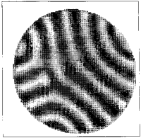
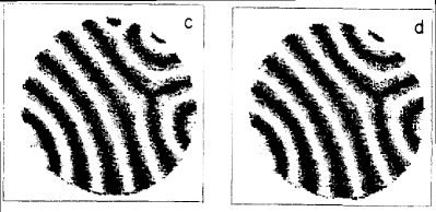
Figure 1: (a) An experimentally observed pattern of rolls in the Rayleigh-Bénard convection, which demonstrates a junction of domain walls (grain boundaries). The pattern corresponds to overcriticality $\varepsilon=1$, see Eq. (23). (b) Similar patterns observed at $\varepsilon=1.8$ (left) and $2$ (right). Reprinted from Ref. [58].

It is relevant to stress that the concept of grain boundaries is known, in a great variety of different realizations, as a very general one in condensed-matter physics [59, 60, 61, 62, 63, 64]. In most cases, the nature of such objects is different from that in thermal convection and other nonlinear dissipative media, Nevertheless, the phenomenology of the grain boundaries in completely different physical systems has many common features.

The DW states were constructed in Ref. [9] as solutions of two coupled real GL equations for amplitudes of PWs connected by the DW. In a particular case, such a solution for a symmetric DW is available in an exact analytical form, see Eqs. (50) and (51) below. It is also demonstrated that the symmetric DW may play the role of a potential well which traps an additional small-amplitude component, in the form of a bright soliton, thus making the structure of the DW more complex, as shown below by Eqs. (72)-(75) and Fig. 5. Further, a newly derived extension of the exact solution in included, for the case when the symmetrically coupled real GL equations include linear-mixing terms (see Eq. (54) below), and a new exact solution for a strongly asymmetric DW, in the case when only one real GL equation includes the diffusion term (second derivative). This solution is given below by Eqs. (64)-(68) and Fig. 4.

At the level of stationary solutions, the same coupled equations which model the grain boundaries in thermal convection predict DWs in optics, as boundaries between spatial or temporal domains occupied by PWs representing different polarizations or different carrier frequencies of light [65]. These equations also produce DW states in binary Bose-Einstein condensates (BECs) composed of immiscible components [66].

Still earlier, approximate solutions similar to DWs were constructed in the framework of a single complex GL equation [67]. Such solutions represent stationary sources of stable PWs with wavenumbers $\pm k$ (see Eq. (19)), emitted in opposite directions (while the above-mentioned “holes” [38] are sinks absorbing colliding PWs with opposite wavenumbers). A special case corresponds to the complex GL equation (12) without the diffusion term, i.e., with $a=0$. In that case, DWs may be approximately reduced to shock waves governed by an effective Burgers equation for a local wavenumber [39]. These results are also included, in a brief form, in Section II. As an extension of the topic, this section also addresses DWs between semi-infinite domains filled by counterpropagating traveling waves (this is possible, in particular, in thermal convection in a layer of a binary fluid heated from below [68, 69, 70, 71]). Furthermore, Section II includes a newly found exact solution for the DW between traveling waves, produced by a system of coupled real GL equations that include group-velocity terms (see Eqs. (85)-(90) below).

Section III summarizes some theoretical results for QP patterns in 2D and 3D nonlinear dissipative media, the study of which was initiated in Ref. [10]. In particular, included are findings for stable QP states produced by combinations of four spatial modes in a laser cavity with different 3D wave vectors [82]. Another possibility to produce a spatially confined four-mode (eight-fold) QP structure, briefly mentioned in Section III, is offered by the overlap of two square-shaped (two-mode) patterns, under the angle of $45^{\text{o}}$, in a transient layer between the patterns [83]. This possibility is a combination of the two main topics considered in this article, viz., DWs and QP patterns.

The article is completed by Section IV, which summarizes basic results and briefly outlines new possibilities in this area.

II DW (domain-wall) patterns

II.1 The source pattern generated by the single complex GL equation

II.1.1 The generic case

To produce approximate solutions to Eq. (12), it is convenient to rewrite it in the Madelung form (6), which yields the following system of equations for real amplitude $A$ and phase $\phi$:

$$\frac{\partial A}{\partial t}=A-A^{3}+\frac{\partial^{2}A}{\partial x^{2}}-A\left(\frac{\partial\phi}{\partial x}\right)^{2}-2b\frac{\partial A}{\partial x}\frac{\partial\phi}{\partial x}-bA\frac{\partial^{2}\phi}{\partial x^{2}},$$ (24)

$$A\frac{\partial\phi}{\partial t}=2\frac{\partial A}{\partial x}\frac{\partial\phi}{\partial x}+A\frac{\partial^{2}\phi}{\partial x^{2}}-cA^{3}+b\frac{\partial^{2}A}{\partial x^{2}}-bA\left(\frac{\partial\phi}{\partial x}\right)^{2}$$ (25)

(recall coefficients of Eq. (12) are subject to normalization conditions (13)). As shown in Ref. [67], a stationary solution of the DW type, which represents a source of PWs emitted in the directions of $x\rightarrow\pm\infty$, can be looked for assuming that the dispersion coefficients $b$ and $a$ are small, and the local amplitude, $A(x)$, and wavenumber, $p(x)\equiv\partial\phi/\partial x$, are slowly varying functions of $x$ (the “nonlinear geometric-optics approximation”, alias the “eikonal approximation”). In the lowest order, all derivatives and dispersion terms may be neglected in Eq. (24), reducing it merely to $A^{2}\approx 1-p^{2}$, cf. Eq. (4). Next, this approximation is substituted in Eq. (25), with the phase taken as

$$\phi(x,t)=-\left(c+(b-c)k^{2}\right)t+\int p(x)dx,$$ (26)

where it is assumed that the asymptotic values of the wavenumber are

$$p\left(x\rightarrow\pm\infty\right)=\pm k$$ (27)

(hence the frequency in expression (26) is the same as in Eq. (19)). Keeping the lowest-order small terms with respect to the small dispersive coefficients and small derivative $dp/dx$ of the slowly varying local wavenumber leads to the following approximate equation:

$$\frac{1-3p^{2}}{1-p^{2}}\frac{dp}{dx}=\left(c-b\right)\left(k^{2}-p^{2}\right).$$ (28)

The DW solution to Eq. (28) can be obtained in an implicit form, which yields $x$ as a function of $p$, satisfying the boundary conditions (27):

$$2k\ln\frac{1-p}{1+p}+\left(1-3k^{2}\right)\ln\frac{k-p}{k+p}=2k\left(b-c\right)\left(1-k^{2}\right)x.$$ (29)

The solution can be easily cast in an explicit form under condition $k^{2}\ll 1$:

$$p(x)\approx k\tanh\left[\left(c-b\right)kx\right].$$ (30)

This form clearly demonstrates that the DW may be indeed construed as an emitter of waves from the center, where $p(x=0)=0$, to $x\rightarrow\pm\infty$, in agreement with Eq. (28). The explicit solutions, as well as the implicit ones (29), constitute a family parameterized by free constant $k$.

In the real GL equation, with $b=c=0$, as well as in the case when the linear and nonlinear dispersions exactly cancel each other, $b=c$, Eq. (28) cannot produce a stationary DW solution. As shown in Ref. [67], in that case initial configurations in the form resembling expression (30), i.e., a step-shaped profile of the local wavenumber, give rise to nonstationary solutions, which may be approximated by means of characteristics and caustics of a quasi-linear evolution equation for $p(x,t)$.

II.1.2 Domain walls as shock waves in the diffusion-free complex GL equation

The consideration of DWs should be performed differently in the special case of the complex GL equation (12) with $a=0$, which does not include the diffusion term. Taking into regard normalization (13), the respective equation takes the form of

$$\frac{\partial u}{\partial t}=u+ib\frac{\partial^{2}u}{\partial x^{2}}-\left(1+ic\right)|u|^{2}u$$ (31)

(in fact, one can additionally rescale coordinate $x$ here, to set $b=\pm 1$). This form of the equation admits free motion of various modes [39, 30]. In this case, the Madelung substitution (6) leads, instead of the amplitude-phase equations (24) and (25), to ones

$$\frac{\partial A}{\partial t}=A-A^{3}-2b\frac{\partial A}{\partial x}\frac{\partial\phi}{\partial x}-bA\frac{\partial^{2}\phi}{\partial x^{2}},$$ (32)

$$A\frac{\partial\phi}{\partial t}=-cA^{3}+b\frac{\partial^{2}A}{\partial x^{2}}-bA\left(\frac{\partial\phi}{\partial x}\right)^{2}.$$ (33)

Further, the lowest approximation of the nonlinear geometric optics, applied to Eq. (32), yields

$$A^{2}\approx 1-b\frac{\partial p}{\partial x}.$$ (34)

The substitution of this in Eq. (33) leads, after simple manipulations (including the division by $A$ and differentiation with respect to $x$, in order to replace $\partial\phi/\partial t$ by $\partial p/\partial t$), to the Burgers equation [39],

$$\frac{\partial p}{\partial t}=bc\frac{\partial^{2}p}{\partial x^{2}}-2bp\frac{\partial p}{\partial x}.$$ (35)

The usual shock-wave solutions of Eq. (35) give rise to a family of DWs with two independent parameters, viz., wall thickness $\xi>0$ and speed $s$, which may be positive or negative:

$$p(x,t)=\frac{s}{2b}-\frac{c}{\xi}\tanh\left(\frac{x-st}{\xi}\right).$$ (36)

The appearance of the second free parameter, $s$, in this solution corresponds to the above-mentioned fact that Eq. (31) admits free motion of patterns produced by this variant of the complex GL equation.

II.2 DWs in systems of real coupled GL equations, as per Ref. [9], and additional analytical findings

II.2.1 The setting

The starting point of the analysis developed in Ref. [9] was a general expression for the distribution of the complex order parameter in the 2D system (e.g., the amplitude of the convective flow):

$$U(x,y;t)=\sum_{l=1}^{N}u_{l}(x,y;t)\exp\left(i\mathbf{n}_{l}\mathbf{\cdot R}\right),$$ (37)

where $\mathbf{R=}\left(x,y\right)$. Equation (37) implies that the order-parameter field is a superposition of $N$ plane-wave modes (often called rolls, in the context of the convection theory) with wave vectors $\mathbf{n}_{l}$, and $u_{l}\left(x,y\right)$ are slowly varying amplitudes of these modes. Stationary states produced by the real GL equations may be looked for in the real form too,

$$u_{l}(x,y)\equiv r_{l}\left(x,y\right),\arg\left(u_{l}\right)=0.$$ (38)

as the evolution of phases $\arg\left(u_{l}\right)$ is trivial in this case.

It is relevant to mention that patterns similar to the rolls (known under the same name) are produced by the Lugiato-Lefever (LL) equation and its varieties. The basic LL equation may be considered as the NLS equation for amplitude $u\left(x,t\right)$ of the optical field in a laser cavity, which includes the linear-loss coefficient, $\gamma>0$, a real cavity-mismatch parameter, $\theta\gtrless 0$, and a constant pump field, $u_{0}$ [40]:

$$\frac{\partial u}{\partial t}=-\gamma u+u_{0}+i\left(|u|^{2}-\theta\right)u+i\frac{\partial^{2}u}{\partial x^{2}}.$$ (39)

Roll patterns were studied in details in various forms of LL models [41, 42, 43]. DWs also occur in these systems [44, 45].

As is illustrated by Fig. 2(a), the simplest possibility of the realization of patterns represented by Eq. (37) is the superposition of $N=2$ modes, each one filling, essentially, a half-plane bounded by the DW. In this case, real amplitudes $r_{1.2}$ are slowly varying functions of only one coordinate, $x$, directed perpendicular to the DW. The respective boundary conditions (b.c.) are

$$r_{1}\left(x\rightarrow-\infty\right)=r_{2}\left(x\rightarrow+\infty\right)=\mathrm{const}\neq 0,$$

$$r_{1}\left(x\rightarrow+\infty\right)=r_{2}\left(x\rightarrow-\infty\right)=0.$$ (40)

The scaled form of stationary (time-independent) coupled real GL equations for slowly varying amplitudes $r_{1}(x)$ and $r_{2}(x)$, corresponding to the bimodal DW configuration defined as per Fig. 2(a) and Eq. (40), are [9] (see also Refs. [14] and [56])

$$D_{1}\frac{d^{2}r_{1}}{dx^{2}}+r_{1}\left(1-r_{1}^{2}-Gr_{2}^{2}\right) = 0,$$ (41)

$$D_{2}\frac{d^{2}r_{2}}{dx^{2}}+r_{2}\left(1-r_{2}^{2}-Gr_{1}^{2}\right) = 0.$$ (42)

Here effective diffusion coefficients are

$$D_{1.2}=\cos^{2}\theta_{1,2}$$ (43)

(see Fig. 2(a)), and $G>0$ is an effective coefficient of the cross-interaction between different plane waves, while the self-interaction coefficient is scaled to be $1$.

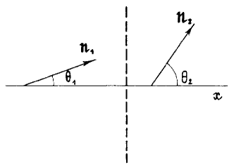
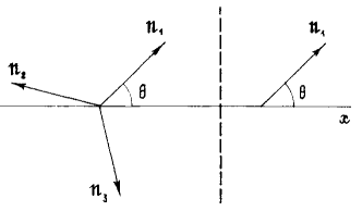
Figure 2: The scheme of the formation of the DW (domain wall) between 2D patterns in the Rayleigh-Bénard convection and similar settings. (a) The DW between plane waves (rolls) with wave vectors oriented under angles $\theta_{1}$ and $\theta_{2}$ with respect to the $x$ axis, see Eq. (37). The respective amplitudes $r_{1,2}(x)$ satisfy Eqs. (41) and (42) and are subject to b.c. (40). The position of the DW is shown by the vertical dashed line. An example of the DW profile is displayed below in Fig. 3(a). (b) The same as in (a), for the DW between hexagons (the triple-mode pattern) and single-mode rolls. The figure is reprinted from Ref. [9].

The symmetric configuration corresponds to Fig. 2(a) with

$$\theta_{1}=-\theta_{2},$$ (44)

which implies $D_{1}=D_{2}\equiv D$, according to Eq. (43). Naturally, the symmetric case plays an important role in the analysis, as shown below.

It is relevant to mention that coupled equations (41) and (42) may be considered as formal equations of motion for a mechanical system with two degrees of freedom, while $x$ plays the role of formal time. This system keeps a constant value of its (formal) Hamiltonian,

$$h=\frac{1}{2}\sum_{j=1,2}\left[D_{j}\left(\frac{dr_{j}}{dx}\right)^{2}+r_{j}^{2}-\frac{1}{2}r_{j}^{4}\right]-\frac{G}{2}r_{1}^{2}r_{2}^{2}.$$ (45)

DW solutions can be readily found as numerical solutions of coupled equations (41) and (42), subject to b.c. (40). A characteristic example of the solution is displayed in Fig. 3(a). In fact, the existence of the DWs in the framework of Eqs. (41) and (42) may be understood as immiscibility of the modes whose amplitudes are produced by these equations. The general condition for the immiscibility, in the present notation, is well known since long ago:

$$G>1,$$ (46)

i.e., the strength of the mutual repulsion of the two components must exceed the strength of their self-repulsion [46].

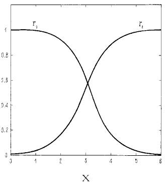
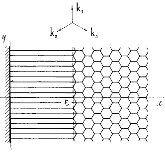
Figure 3: (a) A typical profile of the DW between different plane-wave (roll) families. (b) The structure of the DW between the plane-wave and hexagonal patterns (in this panel, $\mathbf{k}_{1,2,3}$ are identical to $\mathbf{n}_{l}$ in Fig. (37)). The figure is reprinted from Ref. [9].

Hexagonal states in the Rayleigh-Bénard convection are produced by a superposition of three plane waves, with angles $120^{\mathrm{o}}$ between their wave vectors. Such patterns are stable if, in addition to the cubic inter-mode interaction in Eqs. (41) and (42), the respective system of three GL equations for local amplitudes $r_{1,2,3}(x)$ includes resonant quadratic terms:

$$D_{1}\frac{d^{2}r_{1}}{dx^{2}}+r_{1}\left[1-r_{1}^{2}-G\left(r_{2}^{2}+r_{3}^{2}\right)\right]+\nu r_{2}r_{3}=0$$ (47)

plus two complementing equations obtained from Eq. (47) by cyclic permutations of subscripts $\left(1,2,3\right)$, where $\nu$ is a coefficient of the resonant interaction. In the theory of the thermal convection, the quadratic terms represent effects beyond the framework of the basic Boussinesq approximation [93, 94]. Numerical solution of Eq. (47) produces DWs connecting single-mode rolls and the hexagonal pattern [9], see an illustration in Fig. 2(b) and the corresponding pattern displayed in Fig. 3(b). It was also demonstrated that DWs are possible between two bimodal (square-shaped) patterns, each one composed of two plane waves with perpendicular orientations. In that case, the DW appears as a boundary between two half-planes filled by square patterns with different orientations [9, 83], see further details below in Eqs. (125)-(128) and Fig. 9. In Ref. [84], a spatially inhomogeneous model, in which the cross-interaction coefficient is a function of the coordinate, $G=G(x)$, was introduced, making it possible to construct stable DWs between the single- and bimodal patterns.

II.2.2 Basic analytical results from Ref. [9]

An analytically tractable case is the symmetric one, with $D_{1}=D_{2}\equiv D$, and

$$0<G-1\ll 1$$ (48)

(recall that $G>1$ is a necessary condition for the existence of DWs). The analysis makes it possible to reduce these coupled equations to an effective sine-Gordon equation for a slowly varying inter-component phase $\chi(x)$, and thus produce an approximate analytical DW solution with a large width of the transient layer, $L\sim\left(G-1\right)^{-1/2}$ [9]:

$$\left\{\begin{array}[]{c}r_{1}(x)\\ r_{2}(x)\end{array}\right\}\approx\left\{\begin{array}[]{c}\cos\chi(x)\\ \sin\chi(x)\end{array}\right\},\chi=\arctan\left(\exp\left(\sqrt{\frac{G-1}{D}}x\right)\right).$$ (49)

In the particular case of

$$G=3,$$ (50)

the symmetric version of Eqs. (41) and (42) admits an exact DW solution [9]:

$$\left\{\begin{array}[]{c}r_{1}(x)\\ r_{2}(x)\end{array}\right\}=\frac{1}{2}\left\{\begin{array}[]{c}1-\tanh\left(x/\sqrt{2D}\right)\\ 1+\tanh\left(x/\sqrt{2D}\right)\end{array}\right\},$$ (51)

which is obviously compatible with b.c. (40).

II.2.3 New analytical results

Symmetric DWs

Precisely the same real time-independent equations as Eqs. (41) and (42) appear in nonlinear optics as a stationary version of coupled NLS equations in bimodal waveguides, with $r_{1}$ and $r_{2}$ being local amplitudes of electromagnetic waves carrying different wavelengths or different polarizations of light [85]. In the latter case, typical values of $G$ are $2/3$ or $2$, for the linear or circular polarizations of the light, respectively. Other values are possible too, in photonic-crystal waveguides [86]. Similarly, the stationary real equations naturally appear as the time-independent version of coupled Gross-Pitaevskii equations for mean-field wave functions of binary BECs in ultracold atomic gases [87].

Thus, the same solutions as considered here may represent optical DWs [65], as well as DWs separating two immiscible species in the BEC [66]. Further, the coupled equations in optics and BEC models may also include linear mixing between the interacting modes. In particular, this effect is produced by twist applied to the bulk optical waveguide. A similar effect in binary BEC, viz., mutual inter-conversion of two atomic states, which form the binary BEC, may be induced by the resonant radio-frequency field [88]. The respectively modified symmetric system of Eqs. (41) and (42) is

$$D\frac{d^{2}r_{1}}{dx^{2}}+r_{1}\left(1-r_{1}^{2}-Gr_{2}^{2}\right)+\lambda r_{2} = 0,$$ (52)

$$D\frac{d^{2}r_{2}}{dx^{2}}+r_{2}\left(1-r_{2}^{2}-Gr_{1}^{2}\right)+\lambda r_{1} = 0,$$ (53)

where real $\lambda$ is the linear-coupling coefficient. In fact, Eqs. (52) and (53) apply to the Rayleigh-Bénard convection too, in the case when periodic corrugation of the bottom of the convection cell, with amplitude $\sim\lambda$ and wave vector $\mathbf{n}_{1}+\mathbf{n}_{2}$ (see Eq. (37)), gives rise to the effect of the linear cross-gain. Actually, it is used in many laser setups that are similar to thermal convection [89, 90].

The system of Eqs. (52) and (53) with $G=3$ admits an exact DW solution, which is an extension of its counterpart (51):

$$\left\{\begin{array}[]{c}r_{1}(x)\\ r_{2}(x)\end{array}\right\}=\frac{1}{2}\left\{\begin{array}[]{c}\sqrt{1+\lambda}-\sqrt{1-\lambda}\tanh\left(\sqrt{\frac{1-\lambda}{2D}}x\right)\\ \sqrt{1+\lambda}+\sqrt{1-\lambda}\tanh\left(\sqrt{\frac{1-\lambda}{2D}}x\right)\end{array}\right\}.$$ (54)

Due to the action of the linear mixing, b.c. (40) are replaced by

$$r_{1}\left(x\rightarrow-\infty\right)=r_{2}\left(x\rightarrow+\infty\right)=\frac{1}{2}\left(\sqrt{1+\lambda}+\sqrt{1-\lambda}\right),$$

$$r_{1}\left(x\rightarrow+\infty\right)=r_{2}\left(x\rightarrow-\infty\right)=\frac{1}{2}\left(\sqrt{1+\lambda}-\sqrt{1-\lambda}\right).$$ (55)

The extended exact solution given by Eqs. (52)-(55) was not reported in previous publications.

The effect of the confining potential

The above-mentioned realization of the coupled real GL equations in terms of the binary BEC should include, in the general case, a trapping harmonic-oscillator (HO) potential, which is normally used in the experiment [87]. The accordingly modified system of Eqs. (52) and (53) is

$$D\frac{d^{2}r_{1}}{dx^{2}}+r_{1}\left(1-r_{1}^{2}-Gr_{2}^{2}\right)+\lambda r_{2} = \frac{\aleph^{2}}{2}x^{2}r_{1},$$ (56)

$$D\frac{d^{2}r_{2}}{dx^{2}}+r_{2}\left(1-r_{2}^{2}-Gr_{1}^{2}\right)+\lambda r_{1} = \frac{\aleph^{2}}{2}x^{2}r_{2},$$ (57)

where $\aleph^{2}$ is the strength of the OH potential. DW solutions of the system of Eqs. (56) and (57) were addressed in Ref. [91]. A rigorous mathematical framework for the analysis of such solutions in the absence of the linear coupling ($\lambda=0$) was elaborated in Ref. [92].

If the HO trap is weak enough, viz., $\aleph^{2}\ll 4/\left(1-\lambda\right)$, the DW trapped in the OH potential takes nearly constant values, close to those in Eq. (55), in the region of

$$2D/\left(1-\lambda\right)\ll x^{2}\ll 8D/\aleph^{2}.$$ (58)

At $x^{2}\rightarrow\infty$, solutions generated by Eqs. (56) and (57) decay similar to eigenfunctions of the HO potential in quantum mechanics, viz.,

$$r_{1,2} \approx \varrho_{1,2}|x|^{\beta}\exp\left(-\frac{\aleph}{2\sqrt{2D}}x^{2}\right),$$ (59)

$$\beta = \frac{1+\lambda}{\sqrt{2D}\aleph}-\frac{1}{2},$$ (60)

where $\varrho_{1,2}$ are constants. In the case of $\lambda=0$, the asymptotic tails (59) follow the structure of solution (51), i.e., $\varrho_{1}\left(x\rightarrow+\infty\right)=\varrho_{2}\left(x\rightarrow-\infty\right)=0$ and $\varrho_{1}\left(x\rightarrow-\infty\right)=\varrho_{2}\left(x\rightarrow+\infty\right)\neq 0$. On the other hand, the presence of the linear mixing, $\lambda\neq 0$, makes the tail symmetric with respect to the two components, $\varrho_{1}\left(|x|\rightarrow\infty\right)=\varrho_{2}\left(|x|\rightarrow\infty\right)\neq 0$. Note that $\beta=0$ in Eq. (60) with $\lambda=0$ is tantamount to the case when values of $\aleph$ and $D$ in Eqs. (56) and (57) correspond to the ground state of the HO potential.

Exact asymmetric DWs

Another possibility to add a new analytical solution for DWs appears in the limit case of the extreme asymmetry in the system of Eqs. (41) and (42), which corresponds to $D_{2}=0$ and $D_{1}\equiv D>0$, i.e., the DW between two roll families one of which has the wave vector perpendicular to the $x$ axis, see Eq. (43):

$$D\frac{d^{2}r_{1}}{dx^{2}}+r_{1}\left(1-r_{1}^{2}-Gr_{2}^{2}\right)=0,$$ (61)

$$r_{2}\left(1-r_{2}^{2}-Gr_{1}^{2}\right)=0.$$ (62)

Actually, the form of Eq. (62), in which the second derivative drops out, corresponds to the well-known Thomas-Fermi approximation (TF) in the BEC theory. In the framework of the TF approximation, the kinetic-energy term in the Gross-Pitaevskii equation is neglected, in comparison with larger ones, representing a trapping potential and the (self-repulsive) nonlinearity [87]. In the present case, corresponding to $\theta_{2}=90^{\mathrm{o}}$, i.e., $D_{2}=0$ in Eq. (43), is not an approximation, but the exact special case. As concerns the application of Eqs. (41) and (42) to BEC, with the kinetic-energy coefficients $D_{1,2}=\hbar^{2}/\left(2m_{1,2}\right)$ in physical units, where $m_{1,2}$ are atomic masses of the two components of the heteronuclear binary condensate, Eqs. (61) and (62) correspond to a semi-TF approximation, representing a mixture of light (small $m_{1}$) and heavy (large $m_{2}$) atoms, e.g., a ⁷Li–⁸⁷Rb diatomic gas [95].

Obviously, Eq. (62) yields two solutions, viz., either

$$r_{2}=0,$$ (63)

or one featuring to the quasi-TF relation,

$$r_{2}^{2}(x)=1-Gr_{1}^{2}(x).$$ (64)

In the former case, Eq. (61) with $r_{2}=0$ yields a solution in the form of the usual dark soliton, while in the latter case, the substitution of expression (64) in Eq. (61) produces a bright-soliton solution. These solutions may be “dovetailed” at a stitch point,

$$x=x_{0}\equiv-\sqrt{2D}\ln\left(\frac{\sqrt{G}+1}{\sqrt{G}-1}\right),$$ (65)

which is defined by condition $r_{1}^{2}(x)=1/G$ (see Eq. (64). The global form of the solution, which complies with b.c. (40), is

$$r_{1}(x)=\left\{\begin{array}[]{c}-\tanh\left(x/\sqrt{2D}\right),~{}\mathrm{at}~{}-\infty<x<x_{0},\\ \sqrt{\frac{2}{G+1}}\mathrm{sech}\left[\sqrt{\frac{G-1}{D}}\left(x-\xi\right)\right],\mathrm{at}~{}x_{0}<x<+\infty,\end{array}\right.$$ (66)

$$r_{2}(x)=\left\{\begin{array}[]{c}0,~{}\mathrm{at}~{}-\infty<x<x_{0},\\ \sqrt{1-Gr_{1}^{2}(x)},\mathrm{at}~{}x_{0}<x<+\infty.\end{array}\right.$$ (67)

Finally, the virtual center of bright-soliton segment of $r_{1}(x)$ is located at

$$x=\xi\equiv x_{0}-\sqrt{\frac{D}{G-1}}\ln\left(\sqrt{\frac{2G}{G+1}}+\sqrt{\frac{G-1}{G+1}}\right)$$ (68)

(actually, exact solution (66) makes use of the “tail” of the bright soliton in the region of $x\geq x_{0}$, which does not include the central point, $x=\xi$). The distance $x_{0}-\xi$, determined by Eq. (68), defines the effective width of the strongly asymmetric DW. Note that, as seen in Eqs. (65) and (66), this exact solution exists under the condition of $G>1$, which is the above-mentioned immiscibility condition.

It is easy to check that expression (66) satisfies the continuity conditions for $r_{1}(x)$ and $dr_{1}/dx$ at $x=x_{0}$, and expression (67) provides the continuity of $r_{2}(x)$ at the same point. The continuity of $dr_{2}/dt$ at $x=x_{0}$ is not required, as Eq. (62) does not include derivatives. A typical example of the exact solution is displayed, for $D=1$ and $G=2$, in Fig. 4.

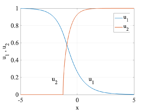
Figure 4: An example of the asymmetric DW, as given by Eqs. (65)-(68), for $D=1$ and $G=2$ (here, $u_{1}$ and $u_{2}$ stand for $r_{1}$ and $r_{2}$ in the analytical solution). Note that the coordinate of the stitch point is, in this case, $x_{0}\approx-1.25$, as per Eq. (65), and the “virtual center” of the bright-soliton segment of $u_{1}(x)$ is located at $\xi\approx-1.80$, as per Eq. (68).

A remarkable fact is that, unlike the above-mentioned exact solutions (51) and (54), which exist solely at $G=3$ (see Eq. (50)), the one given by Eqs. (65)-(68) exists, as a generic one, for all values of $G>1$.

II.2.4 DW-bright-soliton complexes

An exact solution for the composite state

The DW formed by two immiscible PWs may serve as an effective potential for trapping an additional PW mode. To address this possibility, it is relevant to consider the symmetric configuration, with $D_{1}=D_{2}\equiv D$ (see Eq. (43)), and wave vector $\mathbf{k}_{v}$ of the additional PW mode, $v(x)$, directed along the bisectrix of the angle between the DW-forming wave vectors $\mathbf{k}_{1}$ and $\mathbf{k}_{2}$, i.e., along axis $x$ (hence Eq. (43) yields $D_{v}=1$). The corresponding system of three coupled stationary real GL equations is

$$D\frac{d^{2}u_{1}}{dx^{2}}+u_{1}\left(1-u_{1}^{2}-Gu_{2}^{2}-gv^{2}\right) = 0,$$ (69)

$$D\frac{d^{2}u_{2}}{dx^{2}}+u_{2}\left(1-u_{2}^{2}-Gu_{1}^{2}-gv^{2}\right) = 0,$$ (70)

$$\frac{d^{2}v}{dx^{2}}+\left(1-v^{3}-g\left(u_{1}^{2}+u_{2}^{2}\right)\right)v=0,$$ (71)

where $g>0$ is the constant of the nonlinear interaction between components $u_{1,2}$ and $v$.

The system of Eqs. (69)-(71) admits the following exact solution, in the form of the DW of components $u_{1,2}(x)$ coupled to a bright-soliton profile of $v(x)$:

$$\left\{\begin{array}[]{c}u_{1}(x)\\ u_{2}(x)\end{array}\right\}=\frac{1}{2}\left\{\begin{array}[]{c}1-\tanh\left(\sqrt{g-1}x\right)\\ 1+\tanh\left(\sqrt{g-1}x\right)\end{array}\right\},$$ (72)

$$v(x)=\sqrt{2-\frac{3}{2}g}\mathrm{sech}\left(\sqrt{g-1}x\right).$$ (73)

This solution is valid under the condition that coefficients $G$ and $D$ in Eqs. (69) and (70) take the following particular values,

$$G=3-8g+6g^{2},$$ (74)

$$D=\frac{1}{2}\left(3g-1\right).$$ (75)

As is follows from Eq. (73), this solution contains free parameter $g$, which may vary in a narrow interval,

$$1<g<4/3$$ (76)

(see also Eq. (82) below). According to Eqs. (74) and (75), the interval (76) corresponds to coefficients $G$ and $D$ varying in intervals

$$1<G<3;~{}1<D<3/2.$$ (77)

Thus, adding the $v$ component lifts the degeneracy of the exact DW solution (51), which exists solely at $G=3$.

Recall that, in the model of convection patterns, $D$ cannot take values $D>1$, which disagrees with Eq. (77). However, values $D>1$ are relevant for systems of Gross-Pitaevskii equations for the heteronuclear three-component BEC. In the latter case, $D$ is the ratio of atomic masses of the different species which form the triple immiscible BEC. Similarly, $D$ is the ratio of values of the normal group-velocity dispersion of copropagating waves in the temporal-domain realization of the real GL equations in nonlinear fiber optics [65]. In the latter case, values $D>1$ are relevant too.

An example of the DW-bright-soliton complex is displayed in Fig. 5 for $g=7/6$, in which case Eqs. (74) and (75) yield $G=11/6$ and $D=5/4$ (according to Eqs. (74) and (43)).

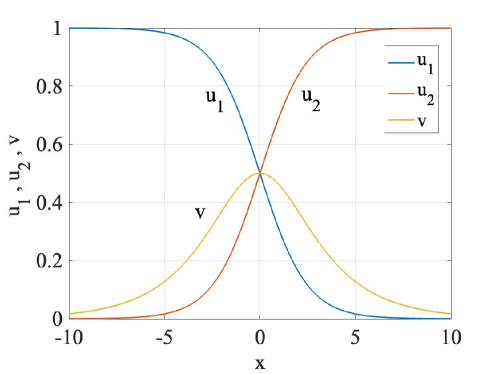
Figure 5: An example of the exact solution for the DW-bright-soliton complex, given by Eqs. (72) and (73), for $g=7/6,G=11/6,$ and $D=5/4$.

The bifurcation of the creation of the composite state in the general case

If relation (74) is not imposed on the interaction coefficients $g$ and $G$, the solution for the composite state cannot be found in an exact form. Nevertheless, it is possible to identify bifurcation points at which component $v$ with an infinitesimal amplitude appears. To this end, Eq. (71) should be used in the form linearized with respect to $v$:

$$\frac{d^{2}v}{dx^{2}}+\left\{1-g\left[u_{1}^{2}(x)+u_{2}^{2}(x)\right]\right\}v=0.$$ (78)

This linear equation can be exactly solved for $u_{1}(x)=u_{2}(x)$ given by expression (51), in the case of $G=3$, while parameters $D$ and $g$ may take arbitrary values. Indeed, using the commonly known solution for the Pöschl-Teller potential in quantum mechanics, it is easy to find that Eq. (78) with the effective potential corresponding to expression (51) gives rise to eigenmodes in the form of

$$v(x)=\mathrm{const}\cdot\left[\mathrm{sech}\left(x/\sqrt{2D}\right)\right]^{\alpha},$$ (79)

at a special value of the interaction coefficient, which identifies the bifurcation producing the composite state:

$$g_{\mathrm{bif}}=D^{-1}\left(1+2D\mp\sqrt{1+2D}\right),$$ (80)

the respective value of power $\alpha$ in expression (79) being

$$\alpha=\sqrt{2\left(1+D\mp\sqrt{1+2D}\right)}.$$ (81)

The values given by Eqs. (80) and (81) with the top sign from $\mp$ correspond to the bifurcation creating a fundamental composite state (the ground state, in terms of the quantum-mechanical analog) at $g>g_{\mathrm{bif}}$, while the bottom sign represents a higher-order bifurcation (alias the second excited state, in the language of quantum mechanics; the first excited state, which is not considered here, is a spatially odd mode). While it is obvious that the fundamental bifurcation provides a stable composite state, it is plausible that the ones produced by higher-order bifurcations are unstable.

Lastly, varying coefficient $D$ of the modes forming the underlying DW between $D=0$ and $D=\infty$ (recall that the convection model corresponds to $D<1,$ while the realizations in BEC and optics admit $D>1$), Eq. (80) demonstrates monotonous variation of the bifurcation point in interval

$$g_{\mathrm{bif}}(D=0)\equiv 1<g_{\mathrm{bif}}<2\equiv g_{\mathrm{bif}}\left(D\rightarrow\infty\right).$$ (82)

It extends interval (76) in which exact composite states with a finite amplitude were found above, see Eqs. (72)-(75).

II.3 Domain walls between traveling waves

II.3.1 The setting

An essential extension of the above results for DWs, produced by coupled equations (41) and (42), was reported in Ref. [96], which addressed a system of coupled GL equations for counter-propagating traveling waves, such as those occurring in binary-fluid convection [68, 69, 70, 71]. The system is composed of two equations of type (12) (subject to normalization (13)), coupled by complex cubic terms with coefficients $G$ and $H$:

$$\frac{\partial u_{1}}{\partial t}+s\frac{\partial u_{1}}{\partial x} = u_{1}+\left(1+ib\right)\frac{\partial^{2}u_{1}}{\partial x^{2}}-\left(1+ic\right)|u_{1}|^{2}u_{1}-\left(G+iH\right)|u_{2}|^{2}u_{1},$$ (83)

$$\frac{\partial u_{2}}{\partial t}-s\frac{\partial u_{1}}{\partial x} = u_{2}+\left(1+ib\right)\frac{\partial^{2}u_{2}}{\partial x^{2}}-\left(1+ic\right)|u_{2}|^{2}u_{2}-\left(G+iH\right)|u_{1}|^{2}u_{2},$$ (84)

where $-s$ and $+s$ are group velocities of the counter-propagating waves, $u_{1}$ and $u_{2}$ (real coefficient $H$ represents the cross-phase modulation (XPM), in terms of optics [85]). A natural approach to constructing DW solutions of the system of Eqs. (83) and (84) is to use the lowest approximation which neglects imaginary parts of coefficients in the equations, but keeps the group-velocity terms. In this approximation, the order parameters are real, $u_{1,2}(x)\equiv r_{1,2}(x)$, obeying the time-independent version of Eqs. (83) and (84):

$$+s\frac{dr_{1}}{dx} = \frac{d^{2}r_{1}}{dx^{2}}+r_{1}\left(1-r_{1}^{2}-Gr_{2}^{2}\right),$$ (85)

$$-s\frac{dr_{2}}{dx} = \frac{d^{2}r_{2}}{dx^{2}}+r_{2}\left(1-r_{2}^{2}-Gr_{1}^{2}\right).$$ (86)

Note that, unlike similar equations (41) and (42), Eqs. (85) and (86) cannot be derived from a formal Hamiltonian, cf. Eq. (45).

II.3.2 A (new) exact analytical solution

To illustrate the structure of the DW state in this approximation, it is relevant to produce a particular exact solution of the system of equations (85) and (86), cf. the above-mentioned solution (51):

$$\left\{\begin{array}[]{c}r_{1}(x)\\ r_{2}(x)\end{array}\right\}=\frac{1}{2}\left\{\begin{array}[]{c}1-\tanh\left(\left(\sqrt{8+s^{2}}+s\right)(x/4\right)\\ 1+\tanh\left(\left(\sqrt{8+s^{2}}+s\right)(x/4\right)\end{array}\right\}.$$ (87)

This solution (which was not reported in earlier works) exists if the following relation holds between the cross-interaction coefficient $G$ and group velocity $v$:

$$G-3=s\left(\sqrt{8+s^{2}}+s\right),$$ (88)

or, inversely,

$$s=\frac{G-3}{\sqrt{2\left(G+1\right)}}.$$ (89)

cf. Eq. (50). It follows from the form of solution (87) and Eqs. (88) and (89) that

$$\mathrm{sgn}(s)=\mathrm{sgn}\left(G-3\right),$$ (90)

i.e., the exact solution represents a sink of traveling waves ($s>0$) for $G>3$, and a source ($s<0$) for $G<3$. Note that the solution of the latter type exists even in the case of $G<1$, when the two components are miscible, cf. Eq. (46). In this case, the mixing is prevented by the opposite group velocities, which pull the components apart.

II.3.3 The sink or source coupled to a bright soliton in an additional component

It is possible to consider a system including the counterpropagating traveling waves coupled to an additional standing one. This is a natural counterpart of the three-component system based on Eqs. (69), (70), and (71). The traveling waves which can trap the additional standing one, $v(x)$, are described by the following generalization of Eqs. (85) and (86):

$$+s\frac{du_{1}}{dx} = \frac{d^{2}u_{1}}{dx^{2}}+u_{1}\left(1-u_{1}^{2}-Gu_{2}^{2}-gv^{2}\right),$$ (91)

$$-s\frac{du_{2}}{dx} = \frac{d^{2}u_{2}}{dx^{2}}+u_{2}\left(1-u_{2}^{2}-Gu_{1}^{2}-gv^{2}\right),$$ (92)

while the equation for the standing component is

$$\frac{d^{2}v}{dx^{2}}+\left(1-v^{2}-g\left(u_{1}^{2}+u_{2}^{2}\right)\right)v=0,$$ (93)

cf. Eq. (71). An exact solution of Eqs. (91)-(93) can be found for free parameters $g$ and $s$:

$$u_{1,2}(x) = \frac{1}{2}\left(1\mp\tanh\left(\sqrt{g-1}x\right)\right),$$ (94)

$$v(x) = \sqrt{2-\frac{3}{2}g}\mathrm{sech}\left(\sqrt{g-1}x\right),$$ (95)

$$G-3 = 2g\left(3g-4\right)+4s\sqrt{g-1},$$ (96)

$$D = \frac{s}{2\sqrt{g-1}}+\frac{1}{2}\left(3g-1\right),$$ (97)

cf. Eqs. (72)-(75). As it is seen from Eq. (96), the interaction with the soliton-shaped standing wave shifts the boundary between the sink and source of the traveling waves off the above-mentioned point, $G=3$.

III Two- and three-dimensional quasiperiodic patterns

Quasicrystals, as stable 3D ordered states of metallic alloys whose atomic lattice is spatially quasiperiodic (QP), were discovered by D. Shechtman et al. [72]. For this discovery, Shechtman was awarded with the Nobel Prize in chemistry (2011). Then, a 2D quasicrystalline structure was also experimentally demonstrated in alloys [73]. The work on this topic remains very active in diverse branches of condensed-matter physics [74, 75, 76], as well as in other physical systems which offer a natural realization of QP patterns, such as photonics [77, 77, 79, 80] and phononics [81].

The objective of this section is to summarize results for stable 2D and 3D patterns with the quasicrystalline structure that were predicted, as stable non-equilibrium dynamical structures (rather than equilibrium states of matter), in nonlinear dissipative media.

III.1 2D octagonal (eight-mode) and decagonal (ten-mode) quasicrystals

Following Ref. [10], generic 2D patterns of a real order parameter, such as one representing the convection flow, are defined by means of complex amplitudes $r_{l}$ of PWs which build them, cf. Eq. (37):

$$U\left(x,y,t\right)=\sum_{l=1}^{2N}u_{l}(t)\exp\left(i\mathbf{n}_{l}\mathbf{\cdot R}\right),$$ (98)

where the set of $2N$ vectors $\mathbf{n}_{l}$ is a star with angles $\pi/N$ between adjacent ones. Note that the vectors satisfy the relation

$$\mathbf{n}_{l+N}=-\mathbf{n}_{l},~{}\mathrm{for}~{}l=1,2,...,N.$$ (99)

Amplitudes $u_{l}(t)$ are, generally speaking, complex variables,

$$u_{l}(t)=A_{l}(t)\exp\left(i\varphi_{l}(t)\right)$$ (100)

(cf. Eq. (6)), subject to constraint $u_{l+N}=u_{l}^{\ast}$, which, along with Eq. (99), secures that the order-parameter distribution (98) is real.

For the lowest-order quasi-crystalline patterns, such as those corresponding to $N=4$ (octagonal) and $N=5$ (decagonal) ones, the phase evolution is trivial, making it possible to disregard $\varphi_{l}$ in Eq. (100). The resulting system of evolution equations for the real amplitudes, including the usual linear gain, $\gamma_{0}>0$, and cubic loss (cf. Eq. (1)), is

$$\frac{dA_{l}}{dt}=\left(\gamma_{0}-\sum_{m=1}^{N}T_{l-m}A_{m}^{2}\right)A_{l}\equiv-\frac{\partial L}{\partial A_{l}},$$ (101)

where $T_{l-m}>0$ are coefficients of the cubic lossy nonlinearity, subject to normalization $T_{0}=1$, and the Lyapunov function is

$$L=-\frac{\gamma_{0}}{2}\sum_{l=1}^{N}A_{l}^{2}+\frac{1}{4}\sum_{l,m=1}^{N}T_{l-m}A_{l}^{2}A_{m}^{2},$$ (102)

cf. Eqs. (2) and (3). Detailed analysis of the results, produced with the help of Eq. (101), was presented in Ref. [10]), see also some preliminary results in Refs. [97] and [98].

Spatially quasiperiodic patterns of the octagonal ($N=4$) and decagonal ($N=5$) types are displayed, respectively, in Figs. 6(a) and 7(a). It is seen that they are built as compositions of rhombuses of different shapes, and the presence of the overall octagonal or pentagonal structure is evident.

Solutions of Eq. (101) for $N=4$ depend on two independent nonlinearity coefficients, $T_{1}=T_{3}$ and $T_{2}$. In this case, there are four distinct stationary solutions which have their stability areas: rolls, with

$$A_{1}=\sqrt{\gamma_{0}},A_{2,3,4}=0;$$ (103)

a square lattice, with

$$A_{1,3}=\sqrt{\gamma_{0}/\left(1+T_{2}\right)},A_{2,4}=0;$$ (104)

an anisotropic rectangular lattice, with the aspect ratio $\tan(\pi/8)=\allowbreak\sqrt{2}-1\approx\allowbreak 0.414$ and amplitudes

$$A_{1,2}=\sqrt{\gamma_{0}/\left(1+T_{1}\right)},A_{3,4}=0;$$ (105)

and the octagonal quasicrystal, with

$$A_{1,2,3,4}=\sqrt{\gamma_{0}/\left(1+2T_{1}+T_{2}\right)}.$$ (106)

In addition to that, Eq. (101) also has a stationary semi-periodic solution, which is quasiperiodic in direction $\mathbf{n}_{2}$ and periodic along $\mathbf{n}_{4}$, with $A_{1}=A_{2}\neq 0,A_{3}\neq 0,$ and $A_{4}=0$. However, the latter solution is completely unstable.

The full stability chart for stationary solutions (103)-(106) can be readily found in an analytical form. It is displayed in Fig. 6(b).

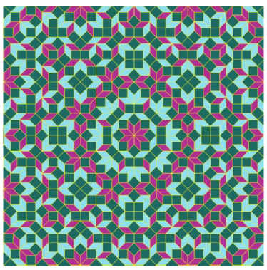
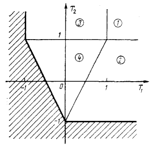
Figure 6: (a) The shape of the octagonal quasiperiodic pattern, reprinted from Ref. [99]. (b) The stability chart for patterns composed of four amplitudes, $A_{1,2,3,4}$, in the plane of nonlinearity coefficients, $T_{1}$ and $T_{2}$, of Eq. (101), reprinted from Ref. [10]. Stability areas of the rolls (103), squares (104), rectangles (105), and octagonal quasicrystal (106) are denoted by encircled numbers 1, 2, 3, and 4, respectively.

For $N=5$, solutions of Eq. (101) also depend on two independent nonlinearity coefficients, $T_{1}=T_{4}$ and $T_{2}=T_{3}$. These equations produce six different species of stable stationary patterns: rolls, with

$$A_{1}=\sqrt{\gamma_{0}},A_{2,3,4,5}=0;$$ (107)

two different species of rectangular lattices:

$$A_{1,2} = \sqrt{\gamma_{0}/\left(1+T_{1}\right)},A_{3,4,5}=0,$$ (108)

$$A_{1,3} = \sqrt{\gamma_{0}/\left(1+T_{2}\right)},A_{2,4,5}=0;$$ (109)

the decagonal quasicrystal:

$$A_{1,2,3,4,5}=\sqrt{\gamma_{0}/\left(1+2T_{1}+2T_{2}\right)};$$ (110)

and two species of semi-periodic patterns, that are quasiperiodic in one direction and periodic in the other:

$$A_{1,3} = \sqrt{\frac{\gamma_{0}\left(1-T_{1}\right)}{1+T_{2}-2T_{1}^{2}}},A_{2}=\sqrt{\frac{\gamma_{0}\left(1+T_{2}-2T_{1}\right)}{1+T_{2}-2T_{1}^{2}}},A_{4,5}=0,$$ (111)

$$A_{1,5} = \sqrt{\frac{\gamma_{0}\left(1-T_{2}\right)}{1+T_{1}-2T_{2}^{2}}},A_{3}=\sqrt{\frac{\gamma_{0}\left(1+T_{1}-2T_{2}\right)}{1+T_{1}-2T_{2}^{2}}},A_{2,4}=0.$$ (112)

In addition to that, there is another semi-periodic solution, with $A_{1}=A_{2}\neq 0$, $A_{3}=A_{4}\neq 0$, and $A_{5}=0$, but it is completely unstable.

The full stability chart for this set of solutions was found too in an analytical form, as shown in Fig. 7(b). In this figure, the constants are

$$\omega_{1}=\frac{\sqrt{5}-1}{2}\approx 0.618,\omega_{2}=\omega_{1}+1.$$ (113)

Note that, unlike the situation for the octagonal setting ($N=4$), displayed in Fig. 6(b), the stability areas for the decagonal ($N=5$) quasicrystal (110) and periodic patterns (108), (109), are not adjacent to each other in Fig. 7(b), being separated by regions of stable semi-periodic states (111) and (112) (recall that all semi-periodic states are unstable in the case of $N=4$).

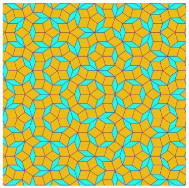
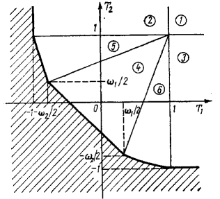
Figure 7: (a) The shape of the decagonal quasiperiodic pattern, reprinted from Ref. [99]. (b) The stability chart for patterns composed of five amplitudes, $A_{1,2,3,4,5}$, in the plane of nonlinearity coefficients, $T_{1}$ and $T_{2}$, of the respective system of equations (101), reprinted from Ref. [10]. Stability areas of the rolls (107), rectangles (108) and (109), decagonal quasicrystal (110), and semi-periodic states (111) and (112), are denoted by encircled numbers 1, 2, 3, 4, 5, and 6, respectively. Constants $\omega_{1}$ and $\omega_{2}$, marked in panel (b), are defined by Eq. (113).

It is relevant to mention that, if higher-order nonlinear terms are added to the system of equations (101), the sharp boundaries between stability areas of different patterns in Figs. 6(b) and 7(b) may be modified. In particular, there may appear narrow strips of bistability (which is impossible in the framework of Eq. (101)), as well as strips populated by more complex patterns, instead of the sharp lines [10].

III.2 Dodecagonal quasicrystals ($N=6$)

In the case of the twelve-mode patterns, corresponding to $N=6$ in Eq. (101), quadratic nonlinearity, with coefficient $\nu>0$, should be included too, as the corresponding set of six wave vectors contains two resonant triads, that may be naturally coupled by the quadratic terms (cf. Eq. (47)):

$$\mathbf{n}_{1}+\mathbf{n}_{5}+\mathbf{n}_{9}=\mathbf{n}_{2}+\mathbf{n}_{6}+\mathbf{n}_{10}=0$$ (114)

(recall that only six wave vectors are actually different, according to Eq. (99)). In this case, the dynamics of phases of the complex amplitudes (6) cannot be disregarded, giving rise to phason modes [100, 101, 102]. Accordingly, Eq. (101) is replaced by a coupled system of evolution equations for the real amplitudes and phases [10]:

$$\frac{dA_{l}}{dt}=\left(\gamma_{0}-\sum_{m=1}^{N}T_{l-m}A_{m}^{2}\right)A_{l}+\nu A_{n+4}A_{n+8}\cos\Phi_{n},$$ (115)

$$A_{l}\frac{d\varphi_{l}}{dt}=-\nu A_{l+4}A_{l+8}\sin\Phi_{l},$$ (116)

$$\Phi_{l}\equiv\varphi_{l}+\varphi_{l+4}+\varphi_{l+8},$$ (117)

with $\varphi_{l}\equiv\varphi_{l-12}$ for $l>12$.

These equations give rise to the following stationary solutions for the dodecagonal quasicrystals, with equal values of real amplitudes $A_{l}$, and the same values of $\Phi_{l}$ for both resonantly coupled triads (114):

$$\cos\Phi_{l}=\pm 1,$$ (118)

$$A_{l}=\pm\left(2Q_{0}\right)^{-1}\left(\nu\pm\sqrt{\nu^{2}+4\gamma_{0}Q_{0}}\right),$$ (119)

$$Q_{0}\equiv 1+2T_{1}+2T_{2}+T_{3}.$$ (120)

The analysis of the stability of these solutions in the framework of Eqs. (115)-(117) demonstrates that they may be stable only under conditions $Q_{0}>0$ (see Eq. (120) and

$$Q_{3}\equiv 1+T_{3}-T_{1}-T_{2}>0.$$ (121)

If these conditions hold, the amplitude of stable quasicrystals exceeds a minimum value,

$$A_{l}\geq A_{\min}\equiv(1/2)\max\left\{\nu/Q_{0},\nu/Q_{3}\right\}.$$ (122)

Further, there is no stability constraint from above for the amplitude, provided that the following combinations of the nonlinearity coefficients are positive:

$$Q_{1,2}\equiv 1-T_{2}\pm\left(T_{1}-T_{3}\right)\geq 0.$$ (123)

Otherwise, the stability imposes the following limit on the amplitude:

$$A\leq A_{\max}\equiv\min\left\{-\nu/Q_{1},-\nu/Q_{2}\right\}$$ (124)

(if only one combination $Q_{1}$ or $Q_{2}$ is negative, only this one determines the upper limit for the stability, as per Eq. (124)).

The existence and stability results for the amplitude of the dodecagonal quasicrystals is summarized in Fig. 8(b). Note that, in the presence of the resonant interaction mediated by the quadratic term in Eq. (115), the solution appears as a subcritical [103] one, with a finite value of the amplitude, at $\gamma_{0}<0$, i.e., when this coefficient represents linear loss, rather than gain.

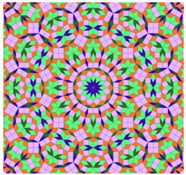
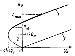
Figure 8: (a) The shape of the dodecagonal quasiperiodic pattern, reprinted from Ref. [99]. (b) The pattern’s amplitude, given by Eq. (119), vs. the strength of the linear gain ($\gamma_{0}>0$) or loss ($\gamma_{0}<0$), reprinted from Ref. [10]. Stable and unstable solutions are represented, respectively, by bold and thin lines. Branches 1, 2 and 3 pertain, severally, to the solutions with $\cos\Phi_{l}=+1$ and $-1$ in Eq. (118). Parameters $Q_{0}$, $A_{\min}$, and $A_{\max}$ are defined as per Eqs. (120), (122), and (124), respectively.

III.3 A quasicrystalline layer between orthogonally oriented square-lattice patterns

While, as shown in Fig. 6(b), square-lattice and octagonal quasiperiodic patterns cannot coexist as stable ones in the system with $N=4$, it was demonstrated in Ref. [83] that a sufficiently broad stripe filled by an effectively stable quasiperiodic pattern may be realized as a transient layer between stable square-lattice patterns mutually oriented under the angle of $45^{\mathrm{o}}$, as schematically shown in Fig. 9(a). For this configuration (which naturally combines the two main topics of the present article, viz., the DWs and QP patterns), one may naturally adopt equal amplitudes corresponding to wave vectors $\mathbf{k}_{3}$ and $\mathbf{k}_{4}$,

$$A_{3}(x)=A_{4}(x)\equiv A(x),$$ (125)

while amplitudes $B_{1}$ and $B_{2}$ related to $\mathbf{k}_{1}$ and $\mathbf{k}_{2}$ are different, the effective diffusion coefficient for the latter one being zero, as per Eq. (43). The corresponding system of stationary real GL equations, naturally extending Eqs. (52), (53), (61), (62), and (101), takes the following form:

$$\frac{1}{2}\frac{d^{2}A}{dx^{2}}+A-A^{3}-\left(T_{1}B_{1}^{2}+T_{1}B_{2}^{2}+T_{2}A^{2}\right)A=0,$$ (126)

$$\frac{d^{2}B_{1}}{dx^{2}}+B_{1}-B_{1}^{3}-\left(2T_{1}A^{2}+T_{2}B_{2}^{2}\right)B_{1}=0,$$ (127)

$$B_{2}-B_{2}^{3}-\left(2T_{1}A^{2}+T_{2}B_{1}^{2}\right)B_{2}=0,$$ (128)

where, like in Eq. (101), $T_{1}$ and $T_{2}$ are coefficients of the cross-interaction between the PW modes with angles, respectively, $45^{\mathrm{o}}$ and $90^{\mathrm{o}}$ between their wave vectors. According to Fig. 6(b), the stability conditions for the spatially uniform square-lattice and octagonal quasicrystalline patterns are, respectively,

$$T_{2} \leq 1,T_{1}\geq T_{2}+1/2,$$ (129)

$$T_{2} \leq 1,T_{1}\leq T_{2}+1/2.$$ (130)

Accordingly, to secure the stability of the background square lattices and a possibility to have a broad transient layer between mutually rotated ones, which is filled by the effectively stable octagonal pattern, it is relevant to choose parameters belonging to the stability area (129), with values close to the stability boundary, $T_{1}=T_{2}+1/2$. An appropriate choice is

$$T_{1,2}\equiv 1-\mu_{1,2},~{}0<\mu_{1,2}\ll 1,$$ (131)

$$\text{with }m\equiv 2\mu_{1}/\mu_{2}<1.$$ (132)

Similar to what is considered above in Eqs. (63) and (64), Eq. (128) obviously splits in two options: $B_{2}=0$, or

$$B_{2}^{2}+2T_{1}A^{2}+T_{2}B_{1}^{2}=1.$$ (133)

In either case, Eqs. (126) and (127) simplify accordingly. The solutions corresponding to $B_{2}=0$ or to Eq. (133) must be “dovetailed” at a stitch point $x=x_{0}$, cf. Eq. (65). An example of the so obtained solutions for amplitudes $A(x)$ and $B_{1,2}(x)$ is displayed in Fig. 9(b).

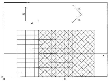
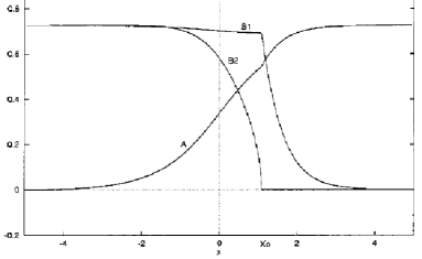
Figure 9: (a) The scheme for building a broad stripe of the octagonal quasicrystalline state as a transient layer between semi-infinite domains filled by square-lattice patterns, mutually rotated by $45^{\mathrm{o}}$. (b) An example of the corresponding solution for amplitudes $A(x)$ and $B_{1,2}(x)$. Parts of the solution corresponding to Eq. (133) or to $B_{2}=0$ are connected at the stitch point $x=x_{0}$. Reprinted from Ref. [83].

III.4 Three-dimensional quasicrystals

A setting which makes it possible to predict a stable quasiperiodic pattern, based on a set of four PW modes, in the 3D space was put forward in Ref. [82]. It originates from the model of a lasing cavity, based on the standard system of coupled Maxwell-Bloch equations. The evolutional variable in this system is time, while the spatial structure is strongly anisotropic, as the field (Maxwell’s) equation in the system contains only the first derivative, $\partial/\partial z$, with respect to the longitudinal coordinate, $z$, and the usual paraxial-diffraction operator, $i\left(\partial_{x}^{2}+\partial_{y}^{2}\right),$acting on the transverse coordinates, $\left(x,y\right)$. As a result, at the lasing threshold components of 3D wave vectors carrying the PW modes,

$$\mathbf{K}=(\mathbf{k},k_{z}),~{}\mathbf{k}\equiv\left(k_{x},k_{y}\right),$$ (134)

satisfy the following dispersion relation, which couples them to the wave’s frequency $\Omega$:

$$\Omega=k^{2}+k_{z}.$$ (135)

Eventually, above the lasing threshold the cubic nonlinearity of the Maxwell-Bloch system may produce a resonant quartet of 3D wave vectors, coupled by condition

$$\mathbf{K}_{1}+\mathbf{K}_{2}=\mathbf{K}_{3}+\mathbf{K}_{4}.$$ (136)

For comparison, in the 2D space the same relation (136), taken close to the threshold, i.e., for nearly equal length of the wave vectors, would imply that the four vectors form a rhombus, and the cubic interaction between the corresponding amplitudes, $u_{1,2,3,4}$, would be represented by usual nonresonant nonlinear terms, essentially the same as in Eq. (101), with $A_{l}$ replaced by $u_{l}$ and $A_{m}^{2}A_{l}$ replaced by the XPM terms, $\left|u_{m}\right|^{2}u_{l}$. However, in the 3D setting the resonance condition (136), combined with the dispersion relation (135), leads to a nontrivial possibility to add four-wave-mixing (FWM) cubic terms to the XPM ones, see below.

Substituting expression (134) for the 3D wave vector in Eqs. (136) and (135) leads to the following elementary exercise in planar geometry: find two pairs of 2D vectors, $\left(\mathbf{k}_{1},\mathbf{k}_{2}\right)$ and $\left(\mathbf{k}_{3},\mathbf{k}_{4}\right)$, satisfying conditions

$$\mathbf{k}_{1}+\mathbf{k}_{2}=\mathbf{k}_{3}+\mathbf{k}_{4},~{}k_{1}^{2}+k_{2}^{2}=k_{3}^{2}+k_{4}^{2}.$$ (137)

An obvious solution of this exercise is plotted in Fig. 10(a).

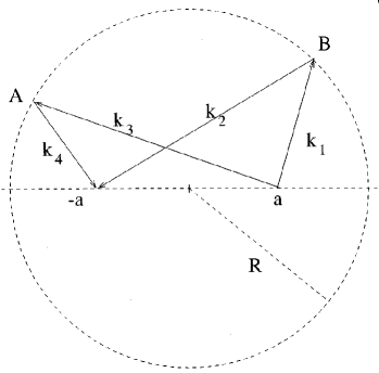
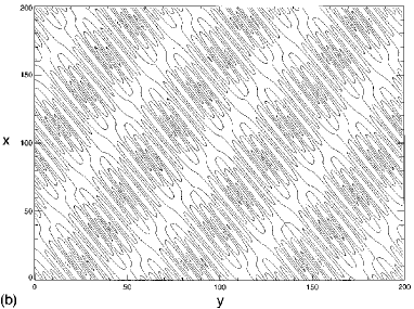
Figure 10: (a) A set of four two-dimensional vectors $\mathbf{k}_{1,2,3,4}$ which solves equations (137). Here, A and B are two arbitrary points belonging to the circumference of arbitrary radius $R$, and $a<R$ is an arbitrary value of coordinate $x$. (b) An example of the three-dimensional quasiperiodic pattern, projected onto the $\left(x,y\right)$ plane. Shown are contour plots of the corresponding distribution of the order parameter, $\mathrm{Re}\left[\sum_{l=1}^{4}u_{l}\cos\left(\mathbf{k}_{l}\cdot\mathbf{R}\right)\right]$, where $u_{l}$ are the complex amplitudes given by Eqs. (141), (142), and (143). In this case, the phases are $\varphi_{1}=\pi,\varphi_{2}=-\pi/2,$ $\varphi_{3}=\pi/7$, while $\varphi_{4}$ is determined by Eq. (142). The angle between vectors $\mathbf{k}_{1}-\mathbf{k}_{2}$ and $\mathbf{k}_{3}-\mathbf{k}_{4}$ is $\pi/5$. The figure is reprinted from Ref. [82].

Once a resonantly coupled quartet of four wave vectors is chosen, the respective system of evolution equations for the corresponding complex amplitudes is [82]

$$\frac{du_{1}}{dt} = \gamma_{0}u_{1}-\left(\left|u_{1}\right|^{2}+2\sum_{l\neq 1}\left|u_{l}\right|^{2}\right)u_{1}-2u_{2}^{\ast}u_{3}u_{4},$$

$$\frac{du_{2}}{dt} = \gamma_{0}u_{2}-\left(\left|u_{2}\right|^{2}+2\sum_{l\neq 2}\left|u_{l}\right|^{2}\right)u_{2}-2u_{1}^{\ast}u_{3}u_{4},$$

$$\frac{du_{3}}{dt} = \gamma_{0}u_{3}-\left(\left|u_{3}\right|^{2}+2\sum_{l\neq 3}\left|u_{l}\right|^{2}\right)u_{3}-2u_{1}u_{2}u_{4}^{\ast},$$

$$\frac{du_{4}}{dt} = \gamma_{0}u_{4}-\left(\left|u_{4}\right|^{2}+2\sum_{l\neq 4}\left|u_{l}\right|^{2}\right)u_{4}-2u_{1}u_{2}u_{3}^{\ast}.$$

In these equations, $\gamma_{0}>0$ is the linear gain, as above, and the last terms represent the above-mentioned FWM effect. Particular values of coefficients in front of nonlinear terms are standard ones which correspond to the XPM and FWM interactions in nonlinear optics [19], unlike general values of coefficients $T_{l-m}$ in Eq. (101). Similar to Eq. (101), the system of equations (LABEL:FWM) admits the presentation in the form of $du_{l}/dt=-$ $\partial L/\partial u_{l}^{\ast}$, with the Lyapunov function

$$L=-\gamma_{0}\sum_{l}\left|u_{l}\right|^{2}+\frac{1}{2}\sum_{l}\left|u_{l}\right|^{4}+2\sum_{l>m}\left|u_{l}\right|^{2}\left|u_{m}\right|^{2}+4\mathrm{Re}\left(u_{1}u_{2}u_{3}^{\ast}u_{4}^{\ast}\right).$$ (139)

Further analysis performed in Ref. [82] had produced two stable stationary solutions of Eqs. (LABEL:FWM). First, this is a simple single-mode state (rolls), with

$$\left|u_{1}\right|^{2}=\gamma_{0},~{}u_{2,3,4}=0.$$ (140)

Next, dodecagonal quasicrystals with equal absolute values of all the four amplitudes are looked for as

$$u_{l}=A\exp\left(i\varphi_{l}\right),$$ (141)

where the phased are locked so that

$$\varphi_{1}+\varphi_{2}-\varphi_{3}-\varphi_{4}=\pi,$$ (142)

and the squared absolute value of the amplitudes is

$$\left|u_{l}\right|^{2}=\gamma_{0}/5,$$ (143)

cf. the rolls solution (140). Note that values of the Lyapunov function (139) for the rolls and 3D quasicrystal are

$$L_{\mathrm{rolls}}=-\gamma_{0}^{2}/2,~{}L_{\mathrm{quasicryst}}=-2\gamma_{0}^{2}/5,$$ (144)

hence the rolls represent the ground state of the system, while the quasicrystal is a metastable state, as its value of $L$ is slightly higher.

An example of the shape of the 3D quasiperiodic solution is displayed, in the projection onto plane $\left(x,y\right)$, in Fig. 10(b). Additional examples can be found in Ref. [82].

Besides these solutions, Eqs. (LABEL:FWM) give rise to another quasiperiodic state, with $\varphi_{1}+\varphi_{2}-\varphi_{3}-\varphi_{4}=0$ and $\left|u_{l}\right|^{2}=\gamma_{0}/9$ (cf. Eqs. (142) and (143)), but it is unstable. Also exist but are unstable two-mode solutions, e.g., ones with $\left|u_{1,2}\right|^{2}=\gamma_{0}/3,u_{3,4}=0$ [82].

IV Conclusion

The aim of this article is to present a concise overview of two important topics in the theory of pattern formation in nonlinear dissipative media, viz., DWs (domain walls) and QP (quasiperiodic) patterns. The topics are selected as those important contributions to which were made in works of Prof. Mikhail Tribelsky. Most results collected in this article may be considered as rather “old” ones, as they had been published ca. 30-35 [9, 10, 12, 29, 39, 48, 51, 58, 65, 67, 68, 94, 98] or 20 [71, 82, 83, 84, 66] years ago. Nevertheless, these results remain relevant in the context of ongoing theoretical and experimental studies in the ever expanding pattern-formation research area. This conclusion is upheld by the fact that the present article includes a few novel exact analytical results, obtained as a relevant addition to the old theoretical findings concerning the DWs in systems of coupled real GL (Ginzburg-Landau) equations [11]. The new results, represented by Eqs. (54), (63)-(68), (72)-(75), and (87)-(90) produce exact solutions for symmetric DWs in the system of real GL equations including linear mixing between the components, the solution for strongly asymmetric DWs in the case when the diffusion term is present only in one GL equation, the three-component composite state including the DW in two components and a bright soliton in the third one, and the particular exact solution for DWs between waves governed by the real GL equations including group-velocity terms with opposite signs.

The significance of the results presented in this brief review is enhanced by the fact that essentially the same coupled equations describe patterns of the DW and QP types not only in thermal convection, but also in nonlinear optics, BEC, and other physical systems. In particular, the pattern formation in BEC of cesium atoms under the action of a temporally-periodic modulation of the nonlinearity (imposed by means of the Feshbach resonance [104]), similar to the Faraday instability, was recently experimentally demonstrated and theoretically modeled in the framework of amplitude equations similar to Eqs. (101) in Ref. [105]. Another novel realization of the pattern formation was proposed for a driven dissipative Bose-Hubbard lattice, that can be implemented in superconducting circuit arrays [106].

It is expected that theoretical and experimental studies along the directions outlined in this article have a potential for further development, which will make it possible to add new findings to the above-mentioned well-established results.

References

- [1] Anisimov, S. I.; Tribelsky, M. I.; Epelbaum, Y. G. Instability of a plane evaporation boundary in the interaction between laser radiation and matter. Zh. Eksp. Teor. Fiz. 1980, 78, 1597-1605.
- [2] Bunkin F. V.; Tribelsky, M. I. Non-resonant interaction of high-power optical radiation with a liquid. Uspekhi Fiz. Nauk. 1980, 130, 193-239.
- [3] Luk’yanchuk, B. S.; Tribelsky, M. I. Anomalous light scattering by small particles. Phys. Rev. Lett. 2006, 97, 263902.
- [4] Tribelsky, M. I.; Flach, S.; Miroshnichenko, A. E.; Gorbach, A. V.; Kivshar, Y. S. Light scattering by a finite obstacle and Fano resonances, Phys. Rev. Lett. 2008, 100, 043903.
- [5] Tribelsky, M. I.; Geffrin, J. M.; Litman, A.; Eyraud, C.; Moreno, F. Small dielectric spheres with high refractive index as new multifunctional elements for optical devices. Sci. Rep. 2015, 5, 12288.
- [6] Miroshnichenko, A. E.; Tribelsky, M. I. Giant in-particle field concentration and Fano resonances at light scattering by high-refractive-index particles. Phys. Rev. A. 2016, 83, 053837.
- [7] Miroshnichenko, A. E.; Tribelsky, M. I. Ultimate absorption in light scattering by a finite obstacle. Phys. Rev. Lett. 2018, 120, 263902.
- [8] Name known as Mikhail/Michael/Michel/Miguel/Michele/Michal/Mikael/Mikkel/Mitxel/… is considered as the oldest masculine name used in modern languages. The meaning of its original form in Hebrew is “who (is) like El (God)?”, which implies a response “no one can be compared to God”.
- [9] Malomed, B. A.; Nepomnyashchy, A. A.; Tribelsky, M. I. Domain boundaries in convection patterns. Phys. Rev. A 1990, 42, 7244-7263.
- [10] Malomed, B. A.; Nepomnyashchy, A. A.; Tribelsky, M. I. Two-dimensional quasiperiodic patterns in nonequilibrium systems. Zh. Eksp. Teor. Fiz. 1989, 96, 688-700.
- [11] Malomed, B. A. New findings for the old problem: Exact solutions for domain walls in coupled real Ginzburg-Landau equations, Phys. Lett. A, in press.
- [12] Malomed, B. A.; Tribelsky, M. I. Bifurcations in distributed kinetic systems with aperiodic instability. Physica D 1984, 14, 67-87.
- [13] Ginzburg, V. L. and Landau, L. D. On the theory of superconductivity. Zhurnal Eksperimentalnoy i Teoreticheskoy Fiziki (USSR) 1950, 20, 1064–1082 (in Russian) [English translation: in Men of Physics, vol. 1. 1965. Oxford: Pergamon Press, pp. 138–167].
- [14] Cross, M. C. Ingredients of a theory of convective textures close to onset. Phys. Rev. A 1982, 25, 1065-1076.
- [15] Eckhaus, W. Studies in Non-Linear Stability Theory, Springer, New York, 1965.
- [16] Wiktor Eckhaus (1930-2000) was born in Poland, where he had survived Holocaust. After WWII, he moved to the Netherlands, where he had eventually become a professor at the Utrecht University.
- [17] Aranson, I. S.; Kramer, L. The world of the complex Ginzburg-Landau equation. Reviews of Modern Physics. 2002, 74, 99-143.
- [18] Malomed, B. A. Complex Ginzburg-Landau equation. In: Encyclopedia of Nonlinear Science, pp. 157-160. A. Scott, editor. New York: Routledge, 2005.
- [19] Kivshar, Y. S.; Malomed, B. A. Dynamics of solitons in nearly integrable systems. Rev. Mod. Phys. 1989, 61, 763-915.
- [20] Arecchi, F. T.; Boccaletti, S.; Ramazza, P. Pattern formation and competition in nonlinear optics. 1999, Physics Reports, 318, 1–83.
- [21] Rosanov, N. N. Transverse patterns in wide-aperture nonlinear optical systems. Progr. Opt. 1996, 35, 1-60.
- [22] Rosanov, N. N. Spatial Hysteresis and Optical Patterns. Springer-Verlag, Berlin, 2002.
- [23] Lega, J. Traveling hole solutions of the complex Ginzburg-Landau equation: a review. Physica D 2001, 152, 269–287.
- [24] Cross, M. C.; Hohenberg, P. C. Pattern-formation outside of equilibrium. Reviews of Modern Physics 1993, 65: 851-1112.
- [25] Ipsen, M.; Kramer, L.; Sorensen, P. G. Amplitude equations for description of chemical reaction-diffusion systems. Phys. Rep. 2000, 337, 193–235.
- [26] Hoyle, R. Pattern Formation: An Introduction to Methods. Cambridge University Press, Cambridge, 2006.
- [27] Malomed, B. A. Strong periodic amplification of solitons in a lossy optical fiber: Analytical results. J. Opt. Soc. Am. B 1994, 11, 1261-1266.
- [28] Berntson, A.; Malomed, B. A. Dispersion-management with filtering. Opt. Lett. 1999, 24, 507-509.
- [29] Malomed, B. A. Evolution of nonsoliton and “quasiclassical” wavetrains in nonlinear Schrödinger and Korteweg - de Vries equations with dissipative perturbations. Physica D 1987, 29, 155-172.
- [30] Sakaguchi, H. Motion of pulses and vortices in the cubic-quintic complex Ginzburg-Landau equation without viscosity. Physica D 2005, 210, 138-148.
- [31] Akhmediev N.; Ankiewicz A., Editors. Dissipative Solitons: From Optics to Biology and Medicine, Springer-Verlag, Springer, 2008.
- [32] Wise, F. W.; Chong, A.; Renninger, W. H. High-energy femtosecond fiber lasers based on pulse propagation at normal dispersion. Laser Phot. Rev. 2008, 2, 58-73.
- [33] T. Ackemann; Firth, W. J.; Oppo, G. L. Fundamentals and applications of spatial dissipative solitons in photonic devices. Adv. At. Mol. Opt. Phys. 2009, 57, 323-421.
- [34] Leblond, H.; Mihalache, D. Models of few optical cycle solitons beyond the slowly varying envelope approximation. Phys. Rep. 2013, 523, 61-126.
- [35] Song, Y. F.; Shi, X. J.; Wu, C. F.; Tang, D. Y.; Zhang, H. Recent progress of study on optical solitons in fiber lasers. Appl. Phys. Rev. 2019, 6, 0213139.
- [36] Hocking L. M.; Stewartson, K. On the nonlinear response of a marginally unstable plane parallel flow to a two-dimensional disturbance. Proc. R. Soc. London Ser. A 1972, 326, 289-313.
- [37] Pereira N. R.; Stenflo, L. Nonlinear Schrödinger equation including growth and damping. Phys. Fluids 1977, 20, 1733-1734.
- [38] Bekki, N.; Nozaki, K.. Formation of spatial patterns and holes in the generalized Ginzburg-Landau equation. Phys. Lett. A 1985. 110, 133-135.
- [39] Malomed, B. A. Stability and grain boundaries in the dispersive Newell-Whitehead-Siegel equation. Physica Scripta 1997, 57, 115-117.
- [40] Lugiato, A. A.; Lefever R. Spatial dissipative structures in passive optical systems, Phys. Rev. Lett. 1987, 58, 2209-2211.
- [41] Oppo G.-L.; Brambilla, M.; Lugiato, L. Formation and evolution of roll patterns in optical parametric oscillators. Phys. Rev. A 1994, 49, 2028-2032.
- [42] Chembo, Y. K.; Menyuk, C. R. Spatiotemporal Lugiato-Lefever formalism for Kerr-comb generation in whispering-gallery-mode resonators. Phys. Rev. A 2013, 87, 053852.
- [43] Huang, S. W.; Yang, J. H.; Yang, S. H.; Yu, M. B.; Kwong, D. L.; Zelevinsky, T.; Jarrahi, M.; Wong, C. W. Globally stable microresonator Turing pattern formation for coherent high-power THz radiation on-chip. Phys. Rev. X 2017, 7, 041002.
- [44] de Valcarcel, G. J.; Staliunas, K. Phase-bistable Kerr cavity solitons and patterns. Phys. Rev. A 2013, 87, 043802.
- [45] Garbin, B.; Wang, Y. D.; Murdoch, S. G.; Oppo, G. L.; Coen, S.; Erkintalo, M. Experimental and numerical investigations of switching wave dynamics in a normally dispersive fibre ring resonator. Eur. Phys. J. D 2017, 71, 240.
- [46] Mineev, V. P. The theory of the solution of two near-ideal Bose gases. Zh. Eksp. Teor. Fiz. 1974, 67, 263-272 (1974) [English translation: Sov. Phys. – JETP 1974, 40, 132-136].
- [47] Petviashvili, V. I.; Sergeev, A. M. Spiral solitons in active media with an excitation threshold. Doklady Akademii Nauk SSSR 1984, 276, 1380–1384 (in Russian).
- [48] Fauve, S.; Thual, O. Solitary waves generated by subcritical instabilities in dissipative systems. Phys. Rev. Lett. 1990, 64, 282-284.
- [49] van Saarloos W.; Hohenberg P. C. Pulses and fronts in the complex Ginzburg-Landau equation near a subcritical bifurcation, Phys. Rev. Lett. 1990, 84, 749-752.
- [50] Hakim, V.; Jakobsen, P.; Pomeau, Y. Fronts vs. solitary waves in nonequilibrium systems. Europhys. Lett. 1990, 11, 19-24.
- [51] Malomed, B. A.; Nepomnyashchy, A. A. Kinks and solitons in the generalized Ginzburg-Landau equation. Phys. Rev. A 1990, 42, 6009-6014.
- [52] Kuramoto, Y.; Tsuzuki, T. Persistent propagation of concentration waves in dissipative media far from thermal equilibrium. Progr. Theor. Phys. 1976, 55, 356-369.
- [53] Sivashinsky, G. I. Nonlinear analysis of hydrodynamic instability in laminar flames—I. Derivation of basic equations. Acta Astronautica 1977, 4, 1177–1206.
- [54] Kuramoto, Y. Diffusion-induced chaos in reaction systems. Progr. Theor. Phys. Supplement 1978, 64, 346–367.
- [55] Cladis, P. E.; Fradin, C.; Finn, P. L.; Brand, H. R. A novel route to defect turbulence in nematics. Mol. Cryst. Liq. Cryst. Sci. Tech. A: Mol. Cryst. Liq. Cryst. 1998, 328, 513-521.
- [56] Manneville, P.; Pomeau, Y. A grain-boundary in cellular structures near the onset of convection. Phil. Mag. A 1983, 48 607-621.
- [57] Haragus, M.; Iooss, G. Bifurcation of symmetric domain walls for the Bénard-Rayleigh convection problem. Arch. Rational Mech. Anal. 2021, 239, 733-781.
- [58] Steinberg, V.; Ahlers, G.; Cannell, D. S. Pattern formation and wave-number selection by Rayleigh-Bénard convection in a cylindrical container. Physica Scripta 1985, 32, 534-547.
- [59] Rohrer, G. S. Grain boundary energy anisotropy: a review. J. Materials Science 2011, 46, 5881-5895.
- [60] Lim, H.; Lee, M. G.; Wagoner, R. H. Simulation of polycrystal deformation with grain and grain boundary effects. Int. J. Plasticity 2011, 27, 1328-1354.
- [61] Rudolph, P. Dislocation patterning and bunching in crystals and epitaxial layers - a review. Cryst. Res. Tech. 2017, 52, 1600171.
- [62] Atxitia, U.; Hinzke, D.; Nowak, U. Fundamentals and applications of the Landau-Lifshitz-Bloch equation. J. Phys. D: Appl. Phys. 2017, 50, 033003.
- [63] Galkina, E. G.; Ivanov, B. A. Dynamic solitons in antiferromagnets. Low Temp. Phys. 2018, 44, 618-633 Published: JUL 2018
- [64] Yao, W.; Wu, B.; Liu, Y. Growth and grain boundaries in 2D materials. ACS NANO 2020, 14, 9320-9346.
- [65] Malomed, B. A. Optical domain walls. Phys. Rev. E 1994, 50, 1565-1571.
- [66] Trippenbach, M.; Góral, K.; Rzażewski, K.; Malomed. B.; Band, Y. B. Structure of binary Bose-Einstein condensates. J. Phys. B: At. Mol. Opt. Phys. 2000, 33, 4017-4031.
- [67] Malomed, B. A. Nonsteady waves in distributed dynamical systems. Physica D 1983, 8, 353-359.
- [68] Cross, M. C. Traveling and standing waves in binary-fluid convection in finite geometries. Phys. Rev. Lett. 1986, 57, 2935-2938.
- [69] Cross, M. C. Structure of nonlinear traveling-wave states in finite geometries, Phys. Rev. A 1988, 38, 3593-3600 (1988).
- [70] Coullet, P.; Frisch, T.; Plaza, F. Sources and sinks of wave patterns. Physica D 1993, 62, 75-79.
- [71] Voss, H. U.; Kolodner, P.; Abel, M.; Kurths, J. Amplitude equations from spatiotemporal binary-fluid convection data. Phys. Rev. Lett. 1999, 83, 3422-3425.
- [72] Shechtman, D.; Blech, I.; Gratias, D.; Cahn, J. Metallic phase with long-range orientational order and no translational symmetry. Phys. Rev. Lett. 1984, 53, 1951-1953.
- [73] Wang, N.; Chen, H.; Kuo, K. Two-dimensional quasicrystal with eightfold rotational symmetry. Phys. Rev. Lett. 1987, 59, 1010-1013.
- [74] Torquato, S. Hyperuniform states of matter. Phys, Rep. 2018, 745, 1-95.
- [75] Steurer, W. Quasicrystals: What do we know? What do we want to know? What can we know? Acta Crystallographica A 2018, 74, 1-11.
- [76] Skjaervo, S. H.; Marrows, C. H.; Stamps, R. L.; Leyderman, L. J. Advances in artificial spin ice. Nature Rev. Phys. 2020, 2, 13-28.
- [77] von Freymann, G; Ledermann, A; Thiel, M.; Staude, I.; Essig, S.; Busch, K.; Wegener, M. Three-dimensional nanostructures for photonics. Adv. Functional Materials 2010, 20, 1038-1052.
- [78] Bellingeri, M.; Chiasera, A.; Kriegel, I.; Scotognella, F. Optical properties of periodic, quasi-periodic, and disordered one-dimensional photonic structures. Optical Materials 2017, 72, 403-421.
- [79] Vardeny, Z. V.; Nahata, A.; Agrawal, A. Optics of photonic quasicrystals. Nature Phot. 2013, 7, 177-187.
- [80] Lu, L.; Joannopoulos, J. D.; Soljacic, M. Topological photonics. Nature Phot. 2014, 8, 821-829.
- [81] Steurer, W.; Sutter-Widmer, D. Photonic and phononic quasicrystals. J. Phys. D: Appl. Phys. 2007, 40, R229-R247.
- [82] Komarova, N.; Malomed, B. A.; Moloney, J. V.; Newell, A. C. Resonant quasiperiodic patterns in a three-dimensional lasing medium. Phys. Rev. A 1997, 56, 803-812.
- [83] Rotstein, H.; Malomed, B. A. A quasicrystallic domain wall in nonlinear dissipative patterns. Physica Scripta 2000, 62, 164-168.
- [84] van Hecke, M.; Malomed, B. A. A domain wall between single-mode and bimodal states and its transition to dynamical behavior in inhomogeneous systems. Physica D 1997, 101, 131-156.
- [85] Kivshar, Y. S.; G. P. Agrawal. Optical Solitons: From Fibers to Photonic Crystals (Academic Press, San Diego, 2003).
- [86] Skorobogatiy, M.; Yang, J. Fundamentals of Photonic Crystal Guiding (Cambridge University Press, Cambridge, 2009).
- [87] Pitaevskii, L. P.; Stringari, S. Bose-Einstein Condensation (Oxford University Press, Oxford, 2003).
- [88] Ballagh, R. J.; Burnett, K.; Scott, T. F. Theory of an output coupler for Bose-Einstein condensed atoms. Phys. Rev. Lett. 1997, 78, 1608-1611.
- [89] Asghari, M.; White, I. H.; Penty, R. V. Wavelength conversion using semiconductor optical amplifiers. J. Lightwave Tech. 1997, 15, R3310-R3313.
- [90] Kim, J.; Laemmlin, M.; Meuer, C.; Bimberg, D.; Eisenstein, G. Theoretical and experimental study of high-speed small-signal cross-gain modulation of quantum-dot semiconductor optical amplifiers. IEEE J. Quant. Elect. 2009, 45, 240-248.
- [91] Merhasin, M. I.; Malomed, B. A.; Driben, R. Transition to miscibility in a binary Bose-Einstein condensate induced by linear coupling. J. Phys. B: At. Mol. Opt. Phys. 2005, 38, 877-892.
- [92] Alama, S.; Bronsard, L.; Contreras, A.; Pelinovsky, D. E. Domains walls in the coupled Gross-Pitaevskii equations. Arch. Rat. Mech. Appl. 2015, 215, 579-615.
- [93] Busse, F. H. The stability of finite amplitude cellular convection and its relation to an extremum principle. J. Fluid Mech. 1967, 30, 625-649.
- [94] Pomeau Y. Front motion, metastability and subcritical bifurcations in hydrodynamics. Physica D 1986, 23, 3-11.
- [95] Marzok, C.; Deh, B.; Courteille, P. W.; Zimmermann, C. Ultracold thermalization of Li and 87Rb. Phys. Rev. A 200, 76, 052704.
- [96] Malomed, B. A. Domain wall between traveling waves. Phys. Rev. E 1994, 50, R3310-R3313.
- [97] Malomed, B. A.; Tribelsky, M. I. On the stability of stationary weakly overcritical patterns in convection and allied problems. Zh. Eksp. Teor. Fiz. (Sov. Phys. JETP) 1987, 92, 539-548.
- [98] Malomed, B. A.; Nepomnyashchy, A. A.; Tribelsky, M. I. Two-dimensional dissipative structures with a quasicrystallic symmetry. Pis’ma Zh. Tekh. Fiz. (Sov. Phys. Tech. Phys. Lett.) 1987, 13, 1165-1167.
- [99] Steurer, W. Twenty years of structure research on quasicrystals. Part I. Pentagonal, octagonal, decagonal and dodecagonal quasicrystals. Zeitschrift für Kristallographie. 2004, 219, 391-446.
- [100] Socolar, J. E. S.; Lubensky, T. C.; Steinhardt, P. J. Phonons, phasons, and dislocations in quasi-crystals. Phys. Rev. B 1986, 34, 3345-3360.
- [101] Yamamoto, A. Crystallography of quasiperiodic crystals. Acta Crystallographica A 1996, 52, 509-560.
- [102] Freedman, B.; Lifshitz, R.; Fleischer, J. W.; Segev, M. Phason dynamics in nonlinear photonic quasicrystals. Nature Materials 2007, 6, 776-781.
- [103] Iooss, G.; Joseph, D. D. Elementary Stability Bifurcation Theory (Springer, New York, 1980).
- [104] Chin, C.; Grimm, R.; Julienne, P.; Tiesinga, E. Feshbach resonances in ultracold gases. Rev. Mod. Phys. 2010, 82, 1225-1286.
- [105] Zhang, Z.; Yao, K.-X.; Feng, L., Hu, J.; Chin, C. Pattern formation in a driven Bose–Einstein condensate. Nature Phys. 2020, 16, 652-656.
- [106] Wang, Z.; Navarrete-Benlloch, C.; Cai, Zi. Pattern formation and exotic order in driven-dissipative Bose-Hubbard systems. Phys. Rev. Lett. 2020, 125, 115301.