NICER study of pulsed thermal X-rays from Calvera: a neutron star born in the Galactic halo?

Abstract

Calvera (1RXS  J141256.0$+$792204) is an isolated neutron star detected only through its thermal X-ray emission. Its location at high Galactic latitude ($b=+37^{\circ}$) is unusual if Calvera is a relatively young pulsar, as suggested by its spin period (59 ms) and period derivative ($3.2\times 10^{-15}$ Hz s^-1). Using the Neutron Star Interior Composition Explorer (NICER), we obtained a phase-connected timing solution spanning four years which allowed us to measure the second derivative of the frequency $\ddot{\nu}=-2.5\times 10^{-23}$ Hz s^-2 and to reveal timing noise consistent with that of normal radio pulsars. A magnetized hydrogen atmosphere model, covering the entire star surface, provides a good description of the phase-resolved spectra and energy-dependent pulsed fraction. However, we find that a temperature map more anisotropic than that produced by a dipole field is required, with a hotter zone concentrated towards the poles. By adding two small polar caps, we find that the surface effective temperature and that of the caps are $\sim$0.1 and $\sim$0.36 keV, respectively. The inferred distance is $\sim$3.3 kpc. We confirm the presence of an absorption line at 0.7 keV associated to the emission from the whole star surface, difficult to interpret as a cyclotron feature and more likely originating from atomic transitions. We searched for pulsed $\gamma$-ray emission by folding seven years of Fermi-LAT data using the X-ray ephemeris, but no evidence for pulsations was found. Our results favour the hypothesis that Calvera is a normal rotation-powered pulsar, with the only peculiarity of being born at a large height above the Galactic disk.

1 Introduction

1RXS  J141256.0$+$792204  is an enigmatic X-ray pulsar with properties that do not fit easily with those of the known classes of isolated neutron stars (NSs). It was discovered in the ROSAT All Sky Survey as a soft X-ray source with high X-to-optical flux ratio, qualifying it as an isolated NS candidate (Rutledge et al., 2008). Its spectral properties resemble those of the small class of thermally emitting NSs known as X-ray Dim Isolated Neutron Stars (XDINSs, also called “Magnificent Seven”, see, e.g., Turolla 2009 for a review).

The XDINSs have long spin periods (3–17 s), very soft X-ray spectra (blackbody temperatures $kT_{\rm BB}\sim 0.05$–$0.1$ keV) often exhibiting broad absorption spectral lines, and X-ray luminosities of $10^{31}$–$10^{32}$ erg s^-1. 1RXS  J141256.0$+$792204  has a slightly hotter thermal spectrum ($kT_{\rm BB}\sim 0.2$ keV) and, like the XDINSs, it does not show any sign of non-thermal X/$\gamma$-ray components (Halpern et al., 2013) nor radio emission (Hessels et al., 2007). For these reasons, it was initially considered as a possible new member of the “Magnificent Seven” class and nicknamed “Calvera”. However, it was later discovered that Calvera has a spin period of 59 ms (Zane et al., 2011) and is spinning down at a rate $\dot{P}=3.2\times 10^{-15}$ s s^-1 (Halpern et al., 2013). These timing parameters give a characteristic age $\tau_{c}=2.9\times 10^{5}$ yr and a dipole magnetic field at the equator $B_{\rm d}=4.4\times 10^{11}$ G, that do not fit with those of the XDINSs, which have $\dot{P}$ of a few 10^-14 s s^-1, $\tau_{c}\sim$1–4 Myr, and $B_{\rm d}\sim 10^{13}-10^{14}$ G.

The X-ray luminosity of Calvera is poorly constrained owing to its unknown distance: $L_{X}\sim 1.3\times 10^{32}d_{\rm kpc}^{2}$ erg s^-1. Its sky position (Galactic coordinates $l=118^{\circ}$, $b=+37^{\circ}$) implies a height of $600\times d_{\rm kpc}$ pc above the Galactic plane. A proper motion of $69\pm 26$ mas yr^-1 in a direction nearly perpendicular and away from the Galactic plane, was measured with Chandra (Halpern & Gotthelf, 2015). The corresponding projected velocity is $\sim 290\times d_{\rm kpc}$ km s^-1. If Calvera has a velocity typical of the bulk of radio pulsars and it was born within the disk scale-height of young massive stars, its distance should be smaller than a few hundreds parsecs. On the other hand, if Calvera is at a much larger distance, considering $\tau_{c}$ as an upper limit on its true age, it must have been born at a height $\gtrsim 90\times d_{\rm kpc}$ pc above the Galactic disk, possibly from the explosion of a high velocity runaway star.

Given its large rotational energy loss rate of $6.1\times 10^{35}$ erg s^-1, some non-thermal X- or $\gamma$-ray emission is expected, but none is seen, with a limit of $L_{\gamma}<8\times 10^{31}d^{2}_{\rm kpc}$ erg s^-1 in the 0.1–300 GeV range (Halpern et al., 2013). While the absence of radio emission could be accounted for by an unfavorable orientation, it is unlikely that the same applies to the $\gamma$-rays, since they are normally emitted by pulsars in very wide beams. If the distance is smaller than one kpc, the $\gamma$-ray luminosity of Calvera is at least two orders of magnitude below that of pulsars with similar spin-down power.

Several authors also discussed possible connections of Calvera with the class of X-ray sources known as central compact objects (CCOs). CCOs are a small group of steady thermal X-ray sources, undetected at radio or $\gamma$-ray energies, and located at the center of supernova remnants (see, e.g., De Luca, 2017). Spin periods in the range 0.1–0.4 s and very small $\dot{P}$ values have been measured in three of them, implying the presence of neutron stars with dipole fields of only (0.3–1)$\times 10^{11}$ G. The lack of an associated SNR led to consider Calvera as a possible “orphaned” (Zane et al., 2011; Halpern, 2011) or aged (Halpern et al., 2013) CCO. The low magnetic field inferred for some CCOs might result from burial of an initially stronger field caused by the fall-back of part of the supernova ejecta (Ho, 2011; Viganò & Pons, 2012; Torres-Forné et al., 2016). As the CCO evolves, the magnetic field would re-emerge on a timescale of $\sim$10⁴ yr while the SNR fades, giving rise to objects with properties similar to those of Calvera.

Here we report on recent X-ray observations of Calvera obtained with the Neutron Star Interior Composition Explorer (NICER) instrument. We computed a neutron star model atmosphere and applied it to derive constraints on the Calvera geometry and temperature distribution through an analysis of phase-resolved spectra and pulse profiles. Using the NICER X-ray data, we also derived a new phase-connected timing solution spanning almost four years and used this ephemeris to search for pulsed $\gamma$-ray emission in the Fermi-LAT data.

2 Observations and data analysis

We analyzed all the data of 1RXS  J141256.0$+$792204 available in the public archive of NICER observations. NICER is an instrument optimized for spectral and timing studies of neutron stars in the 0.2–12 keV range installed on the International Space Station (Gendreau et al., 2016). It is based on 56 coaligned concentrator optics providing a total effective area of 1900 cm² at 1.5 keV. Each concentrator is coupled to a focal plane module (FPM) using a silicon drift detector. Four FPMs have not been working since the beginning of the mission. NICER is a collimated instrument (i.e. it does not provide images) with a field of view 30 arcmin². The timing resolution is better than 300 ns.

The NICER data are split into individual observations (ObsId) spanning at most one day each. Due to the orbital and visibility constraints, each ObsId contains a variable number of disjoint time intervals. The observations of Calvera used here were obtained from 15/9/2017 to 26/2/2021 (see Table 4). Results of the data obtained before October 2018 have been published by Bogdanov et al. (2019).

We reduced the data with the nicerdas software (version 8c) including all the most recently released patches and calibration files (CALDB XTI20210707). As a first step, we filtered the data using the program nicerl2 and the standard cuts. To exclude time intervals of high particle background, we selected data with $K_{p}<5$ and COR_SAX $>1.914~{}K_{p}^{0.684}+0.25$, where $K_{p}$ is an indicator of the effect of the Solar wind activity on the Earth magnetosphere and the condition on COR_SAX excludes parts of the orbit in regions with low cut-off rigidity. To reduce the effect of optical loading in the detectors we also applied the filter FPM$\_$underonly$\_$count $<200$.

These filtered data (about 964 ks of exposure) were used for the timing analysis. We barycentered the arrival times using the JPL DE430 solar system ephemeris and the source position computed for each observation taking into account the proper motion given in Halpern & Gotthelf (2015).

To evaluate the background for the spectral analysis we used the 3C50 model (Remillard et al., 2021). We first extracted the source and background spectra for all the individual observations, excluding time intervals with $|S0_{net}|>0.5$ counts s^-1 and $|hbg_{net}|>0.05$ counts s^-1, where $S0_{net}$ and $hbg_{net}$ are the background-subtracted count rates in the 0.2–0.3 keV and 13–15 keV energy ranges, respectively. By examining the resulting spectra at energies above 4 keV (where the source contribution is negligible), we found that in many cases the model overestimated the background, because it predicted a count rate much higher than the observed one. Therefore, we removed all the observations for which the predicted background count rate in the 4–12 keV range differed by more than 6$\sigma$ from the observed count rate in the same energy range. After all these data selections, resulting in a total exposure of 371 ks, we extracted the total spectrum of the source, as well as the corresponding background spectrum and response files. Moreover, in the total spectrum we removed the data from two particularly noisy FPM (n. 34 and 43).

All the spectra were rebinned with a minimum of three channels per bin, in order to avoid oversampling the instrument energy resolution, and requiring a signal significance of at least 5$\sigma$ in each bin. The spectral analysis was performed using the XSPEC software 12.12.0 including a systematic error of 2%. For the interstellar absorption we used the tbabs model. Errors in the spectral parameters are given at the 90% confidence level.

2.1 Timing analysis

Table 1: Timing parameters

Parameter	$n=3$	$n=4$
T0 (TDB)	58 260.83109832
MJD range	58 014 – 59 272
$\nu$ (Hz)	16.8921479996(2)	16.8921479986(2)
$\dot{\nu}$ ($10^{-13}$ Hz s-1)	–9.3948(1)	–9.3965(2)
$\ddot{\nu}$ ($10^{-23}$ Hz s-2)	–2.54(4)	–0.66(20)
$\dddot{\nu}$ ($10^{-31}$ Hz s-3)	$\dots$	–5.9(6)
$\chi^{2}$/ dof	268.2 / 122	178.7 / 121

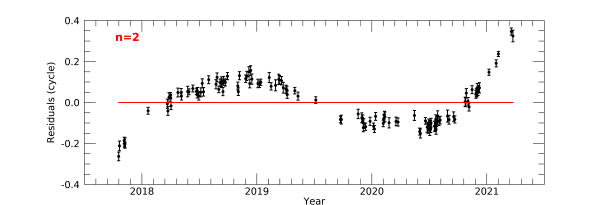
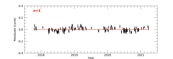
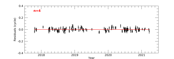
Figure 1: Residuals of the phase-connected timing solutions with only the $\nu$ and $\dot{\nu}$ terms (top) and adding the $\ddot{\nu}$ term (middle). A further term, $\dddot{\nu}$, is included in the fit of the bottom panel.

The X-ray pulsations of Calvera are clearly visible in most of the ObsId with net exposure longer than $\sim$2 ks. To accurately measure the source timing parameters we carried out a phase-coherent timing analysis. Briefly, this consists in fitting the pulse phases with the series expansion

$$\phi(t)=\phi_{0}+\nu(t-t_{0})+\frac{1}{2}\dot{\nu}(t-t_{0})^{2}+\frac{1}{6}\ddot{\nu}(t-t_{0})^{3}+\dots$$ (1)

where $\nu$, $\dot{\nu}$, $\ddot{\nu}$, … are the spin frequency and its time derivatives. The pulse phases were derived by fitting a sine function to the folded light curves in the 0.4–2 keV range. We started by fitting the closely spaced data of May 2018, and then gradually added more and more observations as the decreasing errors on the fit parameters allowed us to keep track of the number of pulse counts. We grouped the ObsId in order to have at least 5 ks in each temporal bin, but we restricted the time span of each group to less than seven days. The resulting ObsId grouping is given in the last column of Table 4. We started the phase fitting with only the $\nu$ and $\dot{\nu}$ terms, obtaining values consistent with those of Bogdanov et al. (2019). However, when we added the data of the second half of 2019, the fit residuals indicated the need of the second and then of the third derivative of the frequency. Figure 1 shows the residuals of the phase-connected timing solutions using the terms of degree $n=2$, $3$ and $4$ in Equation (1). The best-fit parameters, for the cases of the cubic and of the quartic solutions, are given in Table 1.

Figure 2 shows the folded light curve in the 0.4–2 keV energy range (bottom panel) and in three representative energy ranges. The pulse profile is smooth and single-peaked, and the pulsed fraction (PF) increases as a function of the energy: 0.13(1) between 0.4–0.7 keV, 0.24(1) between 0.7–1.2 keV, and 0.31(3) between 1.2–2 keV.

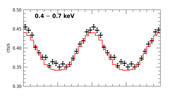
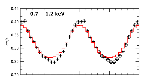
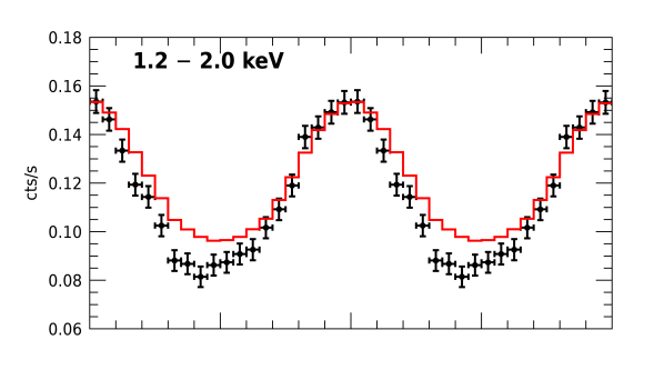
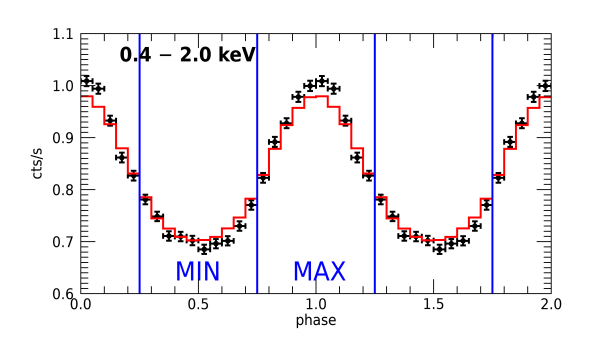
Figure 2: Background-subtracted pulse profiles in three energy ranges (0.4–0.7 keV, upper panel; 0.7–1.2 keV, middle panel; 1.2–2 keV, lower panel), and in the total energy range 0.4–2 keV (bottom panel). The red lines represent the pulse profiles computed with our best fit spectral model (see Section 2.2). The blue vertical lines show the phase intervals used to extract the spectra of the maximum and of the minimum.

2.2 Spectral analysis

For the spectral analysis of Calvera we considered the energy range 0.3–2.5 keV. We found that the phase-averaged spectrum can not be fitted by simple single-component models, such as a blackbody or a power law ($\chi^{2}>1900$ for 63 degrees of freedom, dof). A better fit was found with the sum of two blackbody models with temperatures $kT_{1}\sim 0.15$ keV and $kT_{2}\sim 0.29$ keV, and an absorption edge at $E_{\rm edge}=0.68$ keV ($\chi^{2}/$dof=85.3/59). The best fit is plotted in Figure 3 and all the fit parameters are given in Table 2. Models in which the edge is replaced by two lines were also acceptable, but they involve a larger number of free parameters and will not be considered in the following.

Table 2: Results of phase-averaged spectroscopy

Parameter	Value
$N_{\rm H}$ ($10^{20}$ cm-2)	$1.7\pm 0.4$
$kT_{1}$ (keV)	$0.148\pm 0.008$
$R_{1}^{(a)}$ (km)	$1.24_{-0.11}^{+0.13}$
$kT_{2}$ (keV)	$0.286_{-0.012}^{+0.016}$
$R_{2}^{(a)}$ (km)	$0.26\pm 0.04$
$E_{\rm edge}$ (keV)	$0.68\pm 0.01$
$\tau$	$0.30\pm 0.05$
$F^{(b)}$ ($10^{-12}$ erg cm-2 s-1)	$1.20\pm 0.09$
$\chi^{2}$/ dof	85.3 / 59

Notes. All the errors are at the 90% c.l. for a single interesting parameter.

^a Blackbody emission radius at infinity, for $d=1$ kpc.

^b Observed flux 0.2–10 keV.

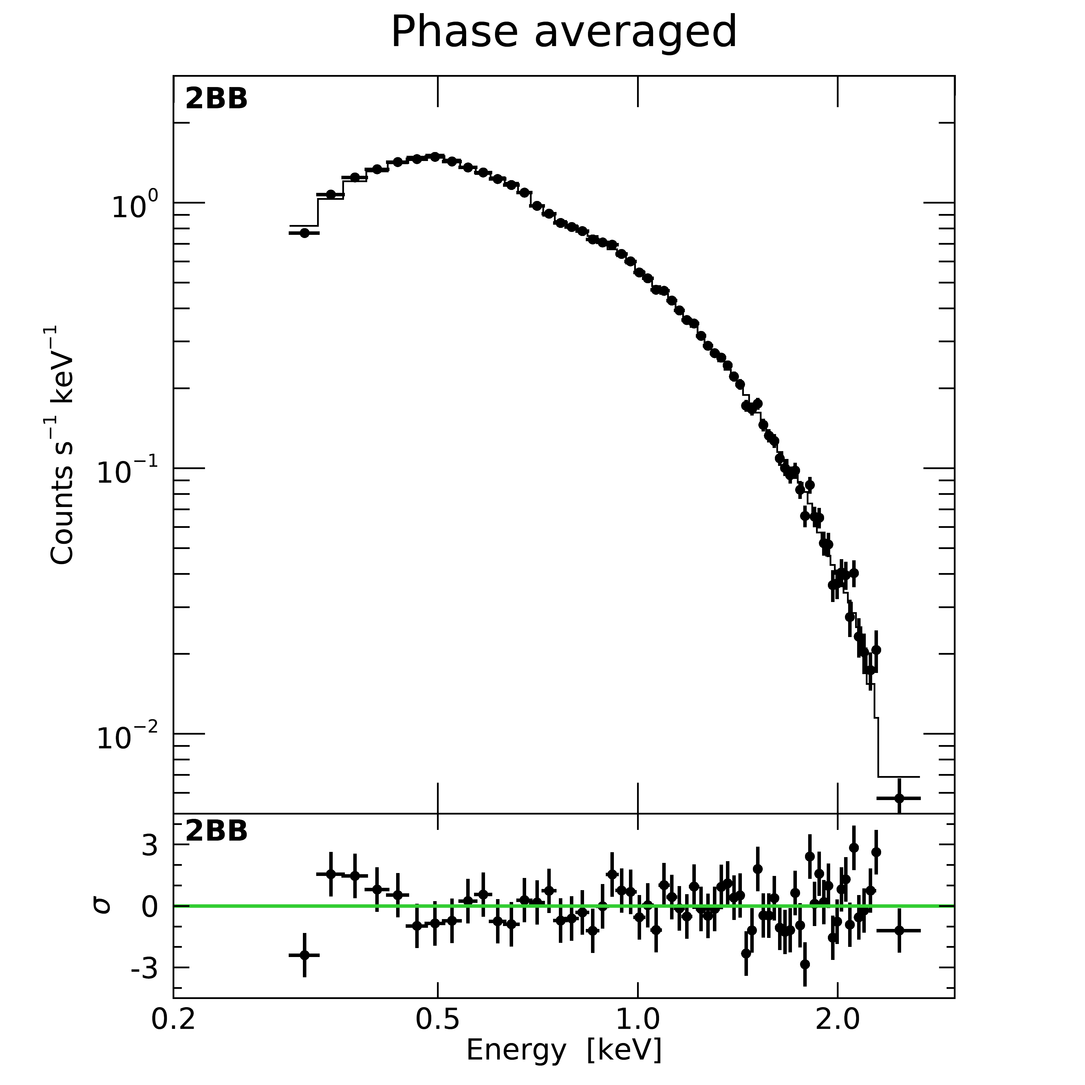
Figure 3: Spectrum of Calvera fitted with two blackbodies + absorption edge (parameters in Table 2).

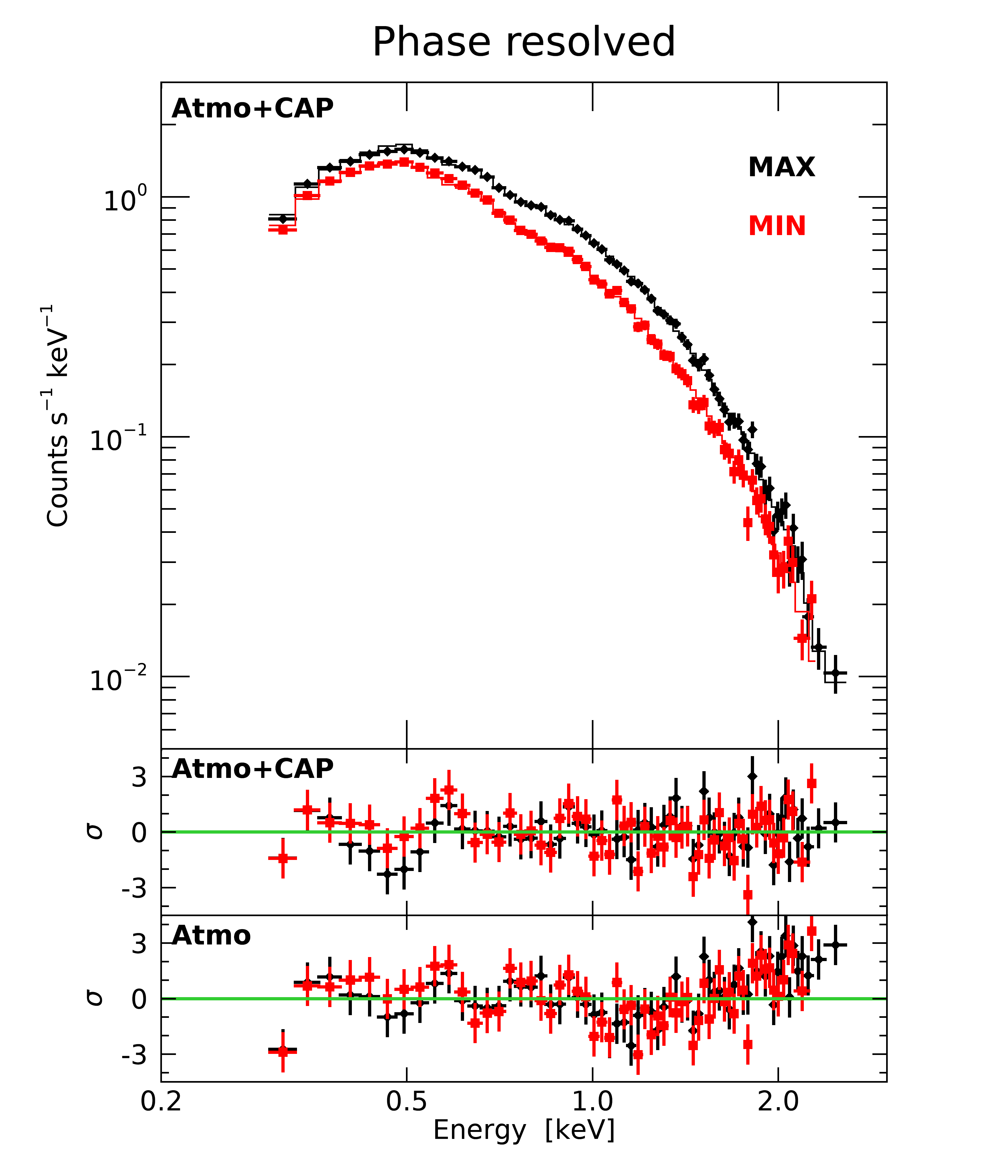
Figure 4: Spectra of the maximum (black) and minimum (red) fitted with our best model (parameters in Table 3).

Given the high statistical quality of the NICER data, rather than trying other thermal models available in XSPEC on the phase-averaged spectrum, we proceeded directly to phase-resolved spectroscopy. For this, we used a neutron star atmosphere model computed ad hoc for the Calvera case as follows.

In order to solve the radiative transfer in the plane-parallel NS atmospheric layer in local thermodynamic equilibrium, we used the code presented by Lloyd (2003), which includes (magnetic) bremsstrahlung and Compton scattering in the source term, with proper expressions for the opacities. The effects of strong magnetic fields are properly dealt with by considering photons polarized both in the ordinary mode (i.e. with the photon electric field oscillating in the $\boldsymbol{kB}$ plane, with $\boldsymbol{k}$ and $\boldsymbol{B}$ the photon propagation direction and the star magnetic field, respectively) and in the extraordinary mode (i.e. with the photon electric field oscillating in the $\boldsymbol{k}\times\boldsymbol{B}$ direction). Each run of the code requires as input parameters the surface gravity $g$ and temperature $T$, as well as the magnetic field strength and inclination with respect to the surface normal at the emission point, and returns the emerging intensities in the two polarization modes as functions of the photon energy and direction with respect to the local normal. The code is designed to treat only pure hydrogen, fully-ionized atmospheres.

As for the mass and radius of the NS, we adopted the values of $M=1.36~{}{\rm M}_{\odot}$ and $R=13$ km (consistent with the equation of state as in e.g., Lattimer & Prakash 2016 and references therein); this corresponds to a surface gravity $\log g=14.11$. We computed the model atmosphere for ten surface patches, equally spaced in $\mu=\cos\theta$, where $\theta$ is the magnetic colatitude. The magnetic field is assumed to be a dipole with polar strength $B_{\rm p}=10^{12}$ G. The polar value of the temperature (as measured at infinity) has been varied by taking six equally spaced values in the range $0.08\,\mathrm{keV}\leq T_{\rm atm}\leq 0.16\,\mathrm{keV}$, and, once $T_{\rm atm}$ is fixed, the temperature distribution in the rest of the NS surface follows that of a dipole, with the corrections by Potekhin et al. (2015). Besides $B_{\rm p}$ (which is held fixed) and $T_{\rm atm}$, each model is characterized by the two angles $\chi$ and $\xi$, which measure the inclination of the line-of-sight and of the dipole axis with respect to the rotation axis, respectively; they are sampled by means of a $19\times 19$ equally-spaced grid ranging, for both angles, from $0^{\circ}$ to $90^{\circ}$.

The spectrum at infinity was computed by collecting all the contributions from the patches that are in view at a certain rotational phase, accounting for general relativistic effects. By integrating over pre-selected phase intervals, we could then obtain the model spectra corresponding to the maximum and minimum of the pulse profile (see the vertical blue lines in Figure 2). These models were used to simultaneously fit the NICER spectra and to derive a single set of the best-fit parameters $T_{\rm atm}$, $\chi$, $\xi$, and the model normalization. Given that the spectral models are computed assuming that the radiation comes from the whole surface, the normalization constant can then be univocally related to the star distance.

Table 3: Results of phase-resolved spectroscopy

Parameter	Atmosphere plus	Atmosphere plus
	H polar caps	BB polar caps
$N_{\rm H}$ ($10^{20}$ cm-2)	$3.1\pm 0.3$	$2.8_{-0.1}^{+0.3}$
$kT_{\rm atm}$ (keV)	$0.103\pm 0.002$	$0.107\pm 0.003$
$d^{(a)}$ (kpc)	$3.27_{-0.16}^{+0.17}$	$3.59\pm 0.22$
$kT_{\rm PC}$ (keV)	$0.358_{-0.035}^{+0}$	$0.84_{-0.26}^{+0.16}$
$R_{\rm PC}^{(b)}$ (m)	$340_{-28}^{+105}$	$63_{-16}^{+66}$
$\chi$ (deg)	$27_{-8}^{+13}$	$25_{-5}^{+11}$
$\xi$ (deg)	$70_{-10}^{+4}$	$66\pm 6$
$E_{\rm edge}^{(c)}$ (keV)	$0.69_{-0.01}^{+0.01}$ / $0.69_{-0.01}^{+0.01}$	$0.69_{-0.01}^{+0.01}$ / $0.69_{-0.01}^{+0.01}$
$\tau^{(c)}$	$0.25_{-0.04}^{+0.04}$ / $0.30_{-0.04}^{+0.04}$	$0.28_{-0.04}^{+0.04}$ / $0.32_{-0.04}^{+0.04}$
$\chi^{2}$/ dof	148.99 / 117	150.19 / 117

Notes. All the errors are at the 90% c.l. for each single parameter.

^a Distance implied by the atmosphere model normalization (for $R_{\rm NS}$ = 13 km adopted in the model computation).

^b Radius of polar cap emission component, for $d$ equal to the best fit value.

^c Values at pulse maximum/minimum.

We found that this model alone (ATMO, in the following) could not properly fit the spectra, due to the presence of an excess at high energy, in addition to the absorption feature already seen in the phase-averaged spectrum (see the bottom panel of Figure 4). The latter was modeled again with an absorption edge, while the high energy excess required an additional hotter component. In order to account for this, we assumed that two, small and hot, polar caps are present, the emission of which was modeled either with a blackbody or with the same magnetized hydrogen atmosphere adopted for the rest of the surface. This further (thermal) component was added to the fit of the phase-resolved spectra, linking the values of $\chi$ and $\xi$ to those of the ATMO component; the cap temperature, $T_{\mathrm{PC}}$, and radius, $R_{\mathrm{PC}}$, are left free to vary (being the caps at the poles, the magnetic field has strength $B_{\mathrm{p}}$ and is normal to the cap surface). In this way we could obtain good fits (see Figure 4) with the parameters reported in Table 3. The temperature and normalization of the emission from the whole star do not depend much on the emission model used for the polar caps (in particular a distance $\sim$3.1–3.8 kpc is obtained in both cases), while the cap temperature is higher by a factor $\simeq$2.3 in the blackbody case. The parameters of the absorption edge were left free to vary as a function of the phase, resulting in marginal evidence for a change in the optical depth.

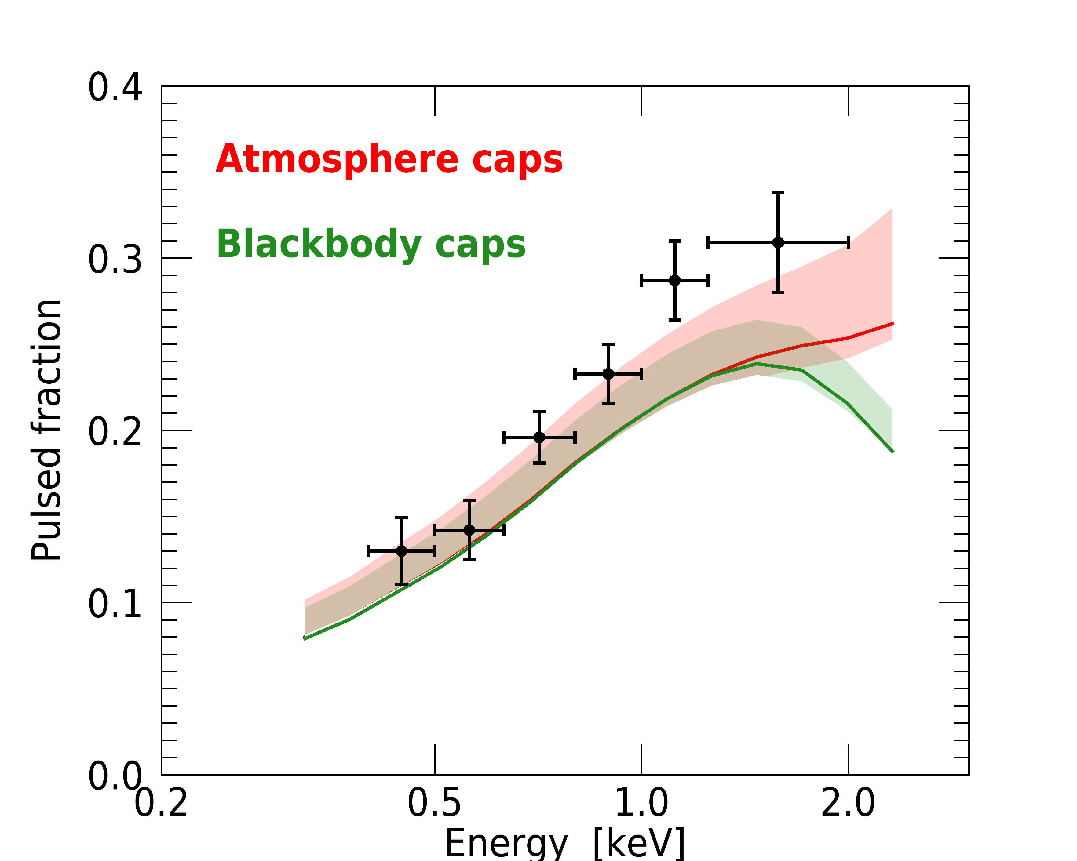
Figure 5: Pulsed fraction as a function of energy. The solid lines shows the pulsed fraction computed from the best fit spectral model (Table 3): an atmosphere model for the entire surface and the hot spots (red), or an atmosphere model for the entire surface and blackbody emission from the hot spots (green). The shadowed areas are obtained in both cases allowing the two angles $\xi$ and $\chi$ to vary within their $90\%$ confidence intervals.

Using the best-fit models obtained from the spectral analysis we can also compute the expected pulse profiles and the PF. Figure 5 shows the PF as a function of the energy in the case of two polar caps modeled with the magnetized hydrogen atmosphere (red solid line) and with the blackbody (green solid line). The two models predict the same PF below $\sim$1 keV, where the bulk of the emission comes from the (full-surface) ATMO component. The colored shadows have been computed letting $\xi$ and $\chi$ free to vary within their 90% confidence level range as obtained from the spectral fit (Table 3). Within this range, we found that the better agreement with the observed values of the energy-dependent PF (black dots in Figure 5) is obtained for $\xi\approx 20^{\circ}$ and $\chi\approx 60^{\circ}$. We then used these angles to compute the expected pulsed profiles in four energy ranges (red lines in Figure 2).

2.3 Timing analysis of Fermi-LAT data

Exploiting the phase-connected timing solution derived from the X-ray data it is possible to search for the presence of a pulsed signal in the Fermi-LAT (Atwood et al., 2009) $\gamma$-ray data with a better sensitivity than in previous similar analysis. We extracted Pass 8 Fermi-LAT events from a circular region with radius of $2^{\circ}$ centered at the position of Calvera and barycentered their times of arrival taking into account the source proper motion, as done for the NICER data. We first considered only the events collected during the time period in which our timing solution is valid. Selecting events of the SOURCE class with energy $E>0.1$ GeV and using the ephemeris of Table 1, we obtained the folded light curve shown in Figure 6 with black dots. This curve is consistent with a constant emission ($\chi^{2}=18.62$ for 19 dof). We then expanded our time baseline to the whole period for which we could ensure the coherency of our timing solution, i.e. we included the events collected after January 2014. This resulted again in an unpulsed signal ($\chi^{2}=15.95$ for 19 dof, see Figure 6, blue dots). We also tried a different energy range ($E>0.3$ GeV) and/or class selection (ULTRACLEANVETO), but also in these cases no evidence for pulsations was found.

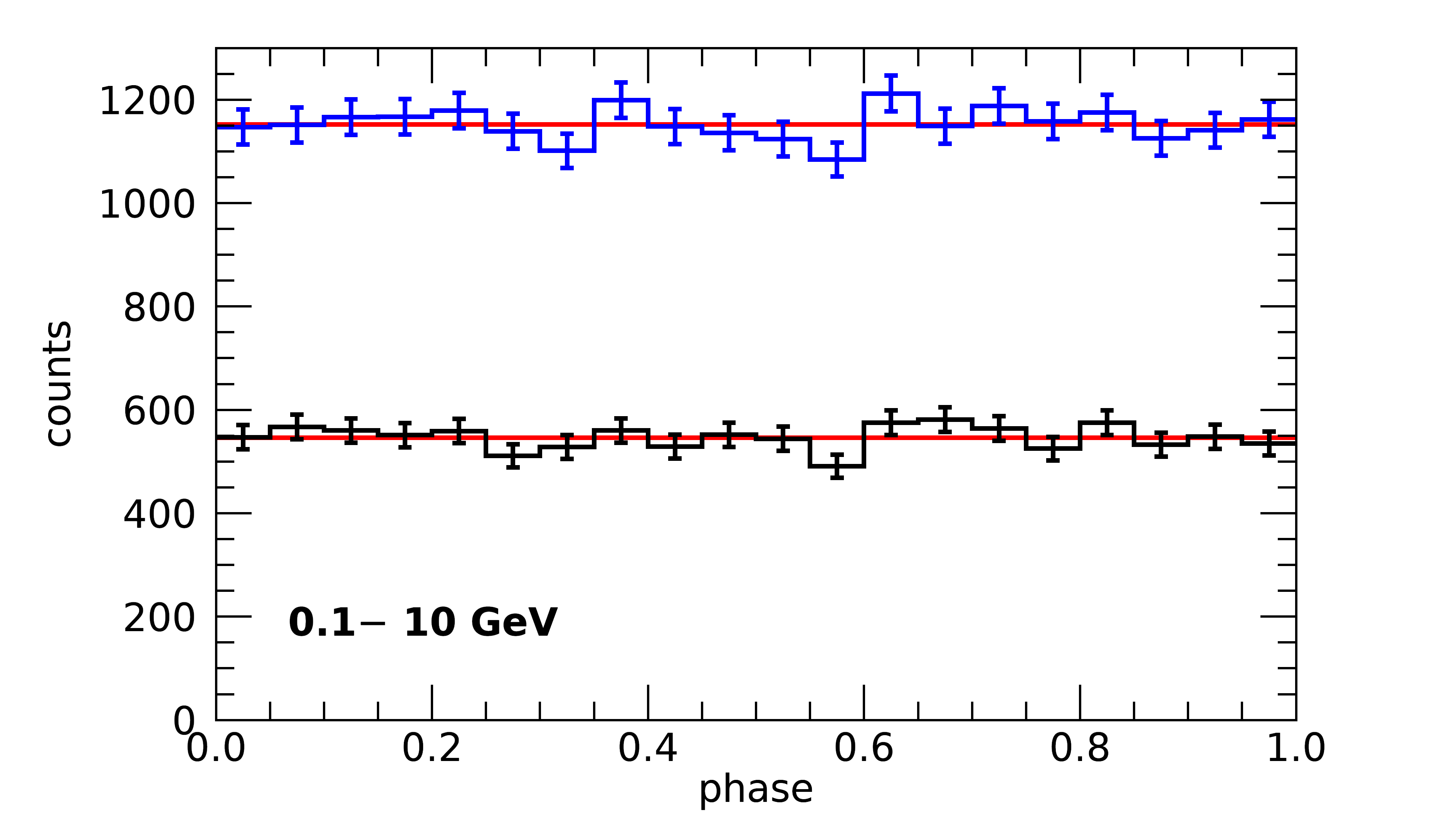
Figure 6: Folded light curves of Fermi-LAT data with energies in 0.1–10 GeV and times of arrival in the range 58 014–59 272 MJD (black dots) or 56 658–59 480 MJD (blue dots). Both are consistent with constant emission (red lines).

3 Discussion

Previous studies of the Calvera X-ray spectrum were based on fits with (the combination of) single temperature thermal components, using either blackbody emission or some of the atmosphere models available in XSPEC. Shevchuk et al. (2009) obtained a good fit to the Chandra phase averaged spectrum with a hydrogen atmosphere model (NSA in XSPEC) and either an absorption edge at 0.64 keV or a Gaussian emission line at 0.53 keV. They favored the latter interpretation on the basis of a higher $\chi^{2}$ improvement. Their best fit normalization, assuming emission from the whole star surface, implied a distance of 3.6 kpc, but no pulsations would be expected in this case. Single temperature thermal models could not fit the higher quality XMM-Newton spectra (Zane et al., 2011; Halpern et al., 2013). The model favored by Zane et al. (2011) consisted of the sum of two blackbodies, with temperatures of $\sim$0.15 and $\sim$0.25 keV, plus a possible absorption edge at $\sim$0.65 keV. If the colder thermal component is from the whole NS surface, the implied distance would be $\sim$5 kpc (for the two blackbody fit) or $\sim$1.5–2 kpc (for the fit with two NSA). Contrary to the single-temperature fits, the models used by Zane et al. (2011) can qualitatively explain the observed pulsations (the same is true for other publicly available atmospheric models explored by Shibanov et al. 2016), but a quantitative modeling of the pulse profile was not carried out by these authors. The phase-averaged spectrum from the NICER data obtained before October 2018 was fitted by Bogdanov et al. (2019) with either a blackbody plus power law or two blackbodies with parameters similar to those of Zane et al. (2011). In both cases the inclusion of an absorption line at $\sim$0.77 keV and an emission line at $\sim$0.55 keV was needed.

Our results are in general agreement with all the findings described above, but our model, having an intrinsically non-uniform temperature distribution, has the advantage of naturally accounting for the observed pulsations. By simultaneously fitting the spectra of two different phase intervals (maximum and minimum), we could obtain some constraints on the angles $\chi$ and $\xi$.

We found that two hotter polar spots, superimposed to the non-isotropic temperature distribution produced by the dipole field, are required to fit the spectra and the pulse profiles. The nature of these spots is uncertain. They can be due to a more complex surface temperature map, like that produced by a strong crustal toroidal field, of which our modeling is just an oversimplified description. In this case, in fact, the insulating effect of the toroidal field allows heat to be conducted to the surface only close to the poles, producing a temperature distribution which is more anisotropic than that induced by a pure dipole Geppert et al. (2006). Alternatively, the spots can be also produced by some form of external heating related to returning magnetospheric currents, as in radiopulsars (Sturrock, 1971; Arons & Scharlemann, 1979, see also Tsygan 2017). If this is the case, it is unlikely that emission from the caps come from an atmosphere in radiative and hydrostatic equilibrium, like that we used to describe the rest of the surface. The radiative properties of bombarded atmospheres are not completely investigated as yet, but there are indications that the spectrum can be described by a single blackbody González-Caniulef et al. (2019). For this reason we modeled the contribution from the caps either with an atmosphere or a blackbody. On the other hand, the fact that the atmospheric model for the caps provides a better agreement with the observed trend of the PF with energy may be taken as indicative that particle bombardment is not substantial and indeed the hot polar region is created by a non-dipolar magnetic field in the crust.

We confirm the presence of a broad absorption feature at $\sim$0.7 keV. The absorption edge we used is the phenomenological model which requires the smallest number of parameters. The line is seen at all rotational phases and it falls at an energy range where most of the flux in our model is contributed by the emission from the entire star surface. This suggests that the line is not related to the polar caps emission component. If interpreted as a cyclotron line from protons on the star surface, a field of $\sim$10¹⁴ G is required, much larger than that inferred for the spin-down dipolar field ($B_{\rm p}=2B_{\rm d}\simeq 9\times 10^{11}$ G). This is in contrast with what observed in the XDINSs, where the spin-down measure agrees rather well with the value of $B$ as derived from the energy of the broad absorption lines (Turolla, 2009). We also note that the option to invoke small-scale, highly magnetized loops as responsible for a proton cyclotron line can work in sources where the feature is strongly phase-dependent (as in the case of SGR 0418+5729 or some of the XDINSs, Tiengo et al., 2013; Borghese et al., 2017), but appears quite untenable for Calvera in the light of our present results. An explanation in terms of an electron cyclotron line is also questionable since the required magnetic field strength in this case is $\sim$7$\times 10^{10}$ G, about one order of magnitude smaller than the surface dipole value. This can be circumvented if the line forms at a height $\sim$2.5$R$ above the surface, so that the magnetic field has decayed to the required value. On the other hand, even then it would be hard to explain how a sufficiently large electron density can be maintained in the inner magnetosphere. A more viable interpretation is that the feature is produced by atomic transitions. H or He transitions in a field $\sim$10¹² G have a maximum energy of $\sim$0.1 and $\sim$0.55 keV, respectively van Kerkwijk & Kaplan (2007); Pavlov & Bezchastnov (2005), below the observed value of $0.7$ keV, but a possibility is that the atmospheric composition comprises heavier elements for which atomic transitions (still poorly known) fall at slightly higher energies.

Thanks to the extensive and dense monitoring performed by NICER, we could obtain a phase connected timing solution extending over 4 years that reveals significant variations in the spin-down rate. These are most likely due to the presence of timing noise, as shown by the residuals in Figure 1. Several indicators have been proposed to quantify the level of timing noise in pulsars (see, e.g. Namkham et al. 2019). One of them is the quantity $\Delta(T_{obs})$, defined as

$$\Delta(T_{obs})={\rm log}\left(\frac{1}{6\nu}|\ddot{\nu}|T_{obs}^{3}\right).$$ (2)

where $T_{obs}$ is the time span of the observations over which $\ddot{\nu}$ is measured (Arzoumanian et al., 1994). Another commonly used measure of the timing noise is given by

$$\sigma_{TN}^{2}=\sigma_{R}^{2}-\sigma_{W}^{2},$$ (3)

where $\sigma_{R}$ is the rms of the residuals of the quadratic time solution and $\sigma_{W}$ is the typical error of the pulse phases.

Our timing solution results in $\Delta_{8}\equiv\Delta(10^{8}\,\mathrm{s})$ = $-0.601\pm 0.007$ and $\sigma_{TN}=6.33$ ms. These values can be compared with those obtained for radio pulsars and other classes of isolated neutron stars. An empirical correlation between $\Delta_{8}$ and $\dot{P}$ predicts $\Delta_{8}=-2.1$ (Arzoumanian et al., 1994), but it has a large scatter, consistent with the value we derived for Calvera. The expected value of $\sigma_{TN}$, according to the scaling relation by Shannon & Cordes (2010), is 5.5 ms. Thus we can conclude that the timing noise of Calvera is higher than the average but still consistent with the distribution of values seen in normal radio pulsars with similar $\dot{P}$.

Zane et al. (2011) reported the presence of diffuse X-ray emission about 13^′ west of Calvera, with spectral properties consistent with a supernova remnant and without counterparts at other wavelengths. For the distance of $d=3.3$ kpc implied by our best fit to the X-ray spectrum, the dimensions of this diffuse emission, $\sim$15$\times$8 pc, are reasonable for a SNR possibly associated to Calvera. However, the measured proper motion indicates that the pulsar is moving toward the putative remnant, rather than away from it. Therefore, we believe there is no physical connection between these two objects.

4 Conclusions

We have analyzed the recent observations of Calvera obtained with NICER to explore the possibility that the observed thermal emission comes from the whole NS surface. We found that our hydrogen atmosphere model, computed for a temperature distribution given by a dipolar magnetic field, is able to well reproduce both the spectra and the pulse profiles, provided that an additional harder component, likely resulting from hot spots at the magnetic poles, is included. We also confirmed the presence of spectral features below 1 keV, that can be fitted, with the minimal number of parameters, as an absorption edge.

Our results demonstrate that the X-ray pulsations can be well reproduced even in the presence of thermal emission from the whole surface. The observed flux implies a distance larger than 3 kpc, which makes Calvera still underluminous in $\gamma$-rays ($<7\times 10^{32}\times d_{\rm 3~{}kpc}^{2}$ erg s^-1, Halpern et al. 2013), but less so than previously suggested.

The most striking property of Calvera is its height above the Galactic disk. The thermal luminosity of $1.4\times 10^{33}$ erg s^-1 (for $d=3.3$ kpc) indicates that $\tau_{c}=P/2\dot{P}\sim 300$ kyr can not be too different from the true age. This supports the idea that Calvera was born in the Galactic halo, most likely from the explosion of a run-away massive star or, possibly, in a more unusual event involving a halo star, such as, e.g., the accretion induced collapse of a white dwarf.

Appendix

The log of NICER observations used for the timing analysis are summarized in Table 4. The table lists the ObsIds, the start time in UTC units, the net exposure time after excluding periods of high particle background as described in Section 2, and the number of the time interval in which each ObsId was grouped for the phase-connected timing analysis.

Table 4: Log of NICER observations

Observation	Start time	Exposure	Grouping
Id	(UTC)	(ks)	Number
1020290102	2017-09-18T05:03:19	1.9	1
1020290103	2017-09-19T07:16:03	0.9	1
1020290104	2017-09-20T03:19:27	1.4	1
1020290105	2017-09-21T09:08:56	2.1	1
1020290106	2017-09-22T04:43:09	5.8	2
1020290107	2017-10-07T07:31:34	10.1	3
1020290108	2017-10-08T02:05:01	9.3	4
1020290109	2017-10-08T23:37:31	16.9	5
1020290110	2017-10-10T00:19:35	6.5	6
1020290120	2017-12-22T02:57:46	8.6	7
1020290122	2018-02-21T00:27:28	7.0	8
1020290123	2018-02-22T07:21:47	2.3	9
1020290124	2018-02-23T09:32:53	1.0	9
1020290125	2018-02-24T16:29:13	1.9	9
1020290126	2018-02-25T03:19:24	1.3	10
1020290127	2018-02-26T00:54:14	2.5	10
1020290128	2018-02-27T05:56:32	4.8	10
1020290129	2018-03-03T01:17:31	11.7	11
1020290130	2018-03-04T03:15:26	8.4	12
1020290131	2018-03-05T01:12:57	8.1	13
1020290135	2018-03-26T10:48:44	2.0	14
1020290136	2018-03-27T03:54:05	4.6	14
1020290143	2018-04-06T01:32:29	7.8	15
1020290144	2018-04-07T00:55:57	6.2	16
1020290150	2018-04-27T00:35:18	5.4	17
1020290152	2018-05-01T00:21:16	12.7	18
1020290153	2018-05-13T05:26:08	9.6	19
1020290154	2018-05-22T22:19:06	0.5	20
1020290155	2018-05-23T01:24:31	1.6	20
1020290156	2018-05-24T02:06:08	2.3	20
1020290157	2018-05-26T03:29:27	3.3	20
1020290158	2018-05-27T01:05:59	6.8	21
1020290159	2018-05-28T00:15:12	6.4	22
1020290160	2018-05-29T00:57:10	1.8	23
1020290161	2018-06-01T01:30:10	1.1	23
1020290162	2018-06-02T02:14:52	0.8	23
1020290163	2018-06-03T13:48:10	0.6	23
1020290164	2018-06-04T02:09:23	0.3	23
1020290165	2018-06-05T02:51:18	0.7	23
1020290166	2018-06-06T20:24:39	0.7	24
1020290167	2018-06-07T05:54:44	0.4	24
1020290168	2018-06-08T01:58:41	4.0	24
1020290169	2018-06-09T02:38:47	1.6	25
1020290171	2018-06-13T06:55:41	2.3	25
1020290172	2018-06-13T23:55:00	2.3	25
1020290174	2018-06-16T04:25:15	5.2	26
1020290176	2018-07-02T03:09:13	3.2	27
1020290177	2018-07-03T05:21:57	3.8	27
1020290183	2018-07-23T15:51:42	0.4	28
1020290184	2018-07-24T07:17:36	0.7	28
1020290185	2018-07-26T17:58:10	2.2	28
1020290186	2018-07-27T01:41:10	1.9	28
1020290188	2018-07-28T23:58:04	5.0	29
1020290189	2018-08-01T11:19:26	2.0	30
1020290190	2018-08-03T15:52:37	0.6	30
1020290191	2018-08-05T09:58:25	0.9	30
1020290192	2018-08-06T07:36:04	2.0	30
1020290194	2018-08-08T00:53:20	7.9	31
1020290198	2018-08-12T00:38:12	5.1	32
1020290199	2018-08-13T01:23:42	7.2	33
1020290204	2018-08-17T00:57:45	7.9	34
1020290206	2018-08-19T00:59:48	6.1	35
1020290207	2018-08-23T03:43:40	0.2	36
1020290208	2018-08-24T00:03:35	2.1	36
1020290209	2018-08-25T00:32:41	4.8	36
1020290211	2018-08-29T07:52:20	3.6	37
1020290212	2018-09-03T08:32:14	1.0	37
1020290213	2018-09-04T20:02:30	1.6	37
1020290215	2018-10-03T01:18:39	6.7	38
1020290216	2018-10-04T11:17:10	3.9	39
1020290217	2018-10-06T11:01:49	1.8	39
1020290218	2018-10-07T00:55:47	3.2	40
1020290219	2018-10-08T04:46:10	0.6	40
1020290220	2018-10-10T21:33:13	0.7	40
1020290221	2018-10-11T00:38:17	1.3	40
1020290225	2018-10-27T05:46:26	1.1	41
1020290226	2018-10-28T07:57:42	2.7	41
1020290227	2018-10-29T05:35:47	3.3	41
1020290228	2018-10-30T03:13:47	3.1	42
1020290229	2018-11-02T05:31:00	0.5	42
1020290230	2018-11-03T06:09:54	2.2	42
1020290233	2018-11-07T10:39:54	5.1	43
1020290234	2018-11-08T11:25:29	1.5	44
1020290235	2018-11-09T05:47:34	1.0	44
1020290236	2018-11-11T14:57:21	2.5	44
1020290238	2018-11-13T00:54:12	5.3	45
1020290239	2018-11-14T12:23:47	0.4	46
1020290240	2018-11-16T09:11:41	1.6	46
1020290241	2018-11-17T06:48:58	1.4	46
1020290242	2018-11-18T01:20:37	2.2	46
1020290245	2018-12-06T04:10:03	5.7	47
1020290247	2018-12-10T23:53:50	6.3	48
1020290249	2018-12-15T08:47:21	7.2	49
1020290256	2019-01-11T00:16:17	5.5	50
1020290257	2019-01-12T08:45:57	1.2	51
1020290258	2019-01-17T06:01:13	1.4	51
1020290259	2019-01-18T02:02:14	4.6	51
1020290263	2019-01-31T04:42:26	5.8	52
1020290269	2019-02-10T08:41:18	5.2	53
1020290270	2019-02-11T17:29:29	0.1	54
1020290271	2019-02-12T02:28:43	4.6	54
1020290272	2019-02-13T06:16:43	0.8	54
1020290275	2019-02-19T01:11:20	7.4	55
1020290276	2019-02-23T22:47:05	0.7	56
1020290277	2019-02-24T00:19:45	3.3	56
1020290278	2019-02-27T09:43:59	1.4	56
1020290279	2019-02-28T05:53:00	1.4	57
2020290201	2019-03-02T01:24:43	0.0	57
2020290202	2019-03-06T07:08:14	2.4	57
2020290203	2019-03-07T01:40:49	2.8	57
2020290204	2019-03-08T11:42:22	5.3	58
2020290205	2019-03-09T01:37:02	9.1	59
2579020101	2019-04-02T14:05:31	9.0	60
2020290210	2019-04-09T16:30:50	0.8	61
2020290211	2019-04-13T09:35:39	4.2	61
2579020201	2019-06-08T03:40:39	9.5	62
2579020305	2019-08-24T23:56:10	7.1	63
2579020306	2019-08-26T16:18:55	3.2	64
2579020307	2019-08-26T23:57:11	1.1	64
2579020308	2019-08-31T15:16:03	0.0	64
2579020309	2019-09-01T19:19:10	1.7	64
2579020401	2019-10-20T14:10:06	5.2	65
2579020404	2019-11-01T04:56:23	5.7	66
2579020405	2019-11-02T00:59:56	7.8	67
2579020407	2019-11-04T00:59:43	7.7	68
2579020409	2019-11-06T00:56:53	6.7	69
2579020410	2019-11-07T00:15:10	1.8	70
2579020411	2019-11-08T00:49:55	4.1	70
2579020412	2019-11-09T09:26:55	0.5	71
2579020413	2019-11-10T08:41:00	0.3	71
2579020414	2019-11-12T00:52:51	0.8	71
2579020415	2019-11-13T09:07:07	2.5	71
2579020416	2019-11-14T02:22:27	0.8	71
2579020417	2019-11-16T02:21:03	1.5	71
2579020419	2019-11-25T16:44:14	0.2	72
2579020420	2019-11-26T09:35:02	1.2	72
2579020421	2019-11-27T01:03:22	0.2	72
2579020422	2019-11-28T06:27:27	3.6	72
2579020501	2019-12-07T08:32:35	1.1	73
2579020502	2019-12-08T03:09:18	3.8	73
2579020503	2019-12-09T05:37:08	4.8	73
2579020505	2019-12-11T00:57:55	7.1	74
2579020508	2019-12-15T00:59:22	7.5	75
2579020512	2020-01-08T02:24:04	6.6	76
2579020513	2020-01-09T00:04:39	3.3	77
2579020514	2020-01-10T08:35:57	2.1	77
2579020516	2020-01-12T02:11:11	9.1	78
2579020517	2020-01-13T01:35:07	3.3	79
2579020518	2020-01-14T09:57:16	1.0	79
2579020519	2020-01-15T03:09:47	1.0	79
2579020520	2020-01-24T14:21:06	0.5	80
2579020521	2020-01-25T08:50:39	1.3	80
2579020601	2020-01-27T04:12:48	1.6	80
2579020602	2020-01-28T01:52:25	2.1	80
2579020607	2020-02-18T00:55:08	6.4	81
2579020609	2020-02-24T08:43:11	6.0	82
3536030107	2020-04-16T08:40:12	5.4	83
3536030114	2020-05-03T00:09:29	9.4	84
3536030115	2020-05-04T00:57:33	2.4	85
3536030116	2020-05-05T00:09:56	1.4	85
3536030117	2020-05-07T18:37:27	1.2	85
3536030118	2020-05-18T11:37:35	1.6	86
3536030119	2020-05-19T06:15:19	0.3	86
3536030120	2020-05-20T00:49:33	0.2	86
3536030121	2020-05-22T00:48:00	1.0	86
3536030122	2020-05-23T00:00:56	3.2	86
3536030123	2020-05-26T03:57:54	1.8	87
3536030124	2020-05-27T04:44:49	1.1	87
3536030125	2020-05-28T02:26:13	2.2	87
3536030126	2020-05-29T09:24:29	1.9	88
3536030127	2020-05-30T02:20:30	3.6	88
3536030129	2020-06-01T00:46:07	11.2	89
3536030131	2020-06-03T00:50:29	10.0	90
3536030132	2020-06-04T00:04:45	5.0	91
3536030134	2020-06-06T04:43:17	7.6	92
3536030135	2020-06-07T00:37:54	9.3	93
3536030136	2020-06-08T01:31:43	6.0	94
3536030201	2020-06-19T03:44:54	6.4	95
3536030203	2020-06-21T13:14:59	5.0	96
3536030204	2020-06-21T23:55:06	9.9	97
3536030205	2020-06-23T02:17:35	7.7	98
3536030206	2020-06-23T23:54:29	5.8	99
3536030207	2020-06-25T03:51:26	2.1	100
3536030208	2020-06-26T09:04:34	4.8	100
3536030209	2020-06-27T09:48:52	4.6	101
3536030210	2020-06-27T23:46:47	1.8	101
3536030211	2020-06-29T03:39:25	6.4	102
3536030212	2020-07-01T18:56:56	0.6	103
3536030213	2020-07-02T21:46:37	0.0	103
3536030214	2020-07-03T14:21:23	1.7	103
3536030215	2020-07-04T01:16:51	3.5	103
3536030218	2020-07-07T01:57:59	10.8	104
3536030224	2020-07-26T22:42:02	0.3	105
3536030225	2020-07-28T05:41:30	0.2	105
3536030226	2020-07-29T20:25:51	0.5	105
3536030227	2020-07-30T11:55:12	1.6	105
3536030228	2020-07-31T09:36:11	3.5	105
3536030229	2020-08-01T10:19:31	1.5	106
3536030230	2020-08-02T09:34:25	0.8	106
3536030231	2020-08-03T10:22:11	0.3	106
3536030232	2020-08-07T07:13:42	2.4	106
3536030234	2020-08-18T14:38:08	1.4	107
3536030235	2020-08-19T00:59:34	3.7	107
3536030236	2020-08-20T03:42:17	0.4	108
3536030237	2020-08-20T23:38:54	1.5	108
3536030238	2020-08-22T02:16:38	0.9	108
3536030239	2020-08-24T01:50:23	3.6	108
3536030309	2020-09-22T22:38:06	0.3	109
3536030310	2020-09-23T03:16:29	2.3	109
3536030311	2020-09-24T21:01:30	0.6	109
3536030312	2020-09-25T01:39:45	3.1	109
3536030313	2020-09-26T00:54:51	5.0	110
3536030314	2020-09-27T14:06:46	0.5	111
3536030315	2020-09-28T00:55:42	4.0	111
3536030316	2020-09-29T06:22:00	1.0	111
3536030317	2020-10-02T19:31:06	0.3	112
3536030318	2020-10-03T10:57:26	4.5	112
3536030319	2020-10-04T17:57:14	2.5	112
3536030320	2020-10-05T00:08:51	3.2	113
3536030321	2020-10-10T10:15:53	1.8	113
3536030401	2020-10-16T16:22:35	6.1	114
3536030402	2020-10-24T21:14:12	0.7	115
3536030403	2020-10-25T01:59:55	0.6	115
3536030404	2020-10-28T21:17:54	0.7	115
3536030405	2020-10-29T03:31:59	4.9	115
3536030406	2020-10-30T02:30:30	8.4	116
3536030407	2020-11-01T09:04:56	5.4	117
3536030408	2020-11-02T00:24:41	5.3	118
3536030409	2020-11-04T01:55:11	11.1	119
3536030411	2020-11-06T05:01:56	7.3	120
3536030413	2020-11-09T00:45:36	5.6	121
3536030502	2020-12-09T00:42:47	11.0	122
3536030507	2021-01-01T01:37:17	9.3	123
3536030509	2021-01-08T02:13:42	14.1	124
3536030602	2021-02-18T09:14:55	9.7	125
3536030604	2021-02-23T08:13:01	5.7	126

References

- Arons & Scharlemann (1979) Arons, J., & Scharlemann, E. T. 1979, ApJ, 231, 854, doi: 10.1086/157250
- Arzoumanian et al. (1994) Arzoumanian, Z., Nice, D. J., Taylor, J. H., & Thorsett, S. E. 1994, ApJ, 422, 671, doi: 10.1086/173760
- Atwood et al. (2009) Atwood, W. B., Abdo, A. A., Ackermann, M., et al. 2009, ApJ, 697, 1071, doi: 10.1088/0004-637X/697/2/1071
- Bogdanov et al. (2019) Bogdanov, S., Ho, W. C. G., Enoto, T., et al. 2019, ApJ, 877, 69, doi: 10.3847/1538-4357/ab1b2e
- Borghese et al. (2017) Borghese, A., Rea, N., Coti Zelati, F., et al. 2017, MNRAS, 468, 2975, doi: 10.1093/mnras/stx632
- De Luca (2017) De Luca, A. 2017, in Journal of Physics Conference Series, Vol. 932, Journal of Physics Conference Series, 012006, doi: 10.1088/1742-6596/932/1/012006
- Gendreau et al. (2016) Gendreau, K. C., Arzoumanian, Z., Adkins, P. W., et al. 2016, in Society of Photo-Optical Instrumentation Engineers (SPIE) Conference Series, Vol. 9905, Space Telescopes and Instrumentation 2016: Ultraviolet to Gamma Ray, ed. J.-W. A. den Herder, T. Takahashi, & M. Bautz, 99051H, doi: 10.1117/12.2231304
- Geppert et al. (2006) Geppert, U., Küker, M., & Page, D. 2006, A&A, 457, 937, doi: 10.1051/0004-6361:20054696
- González-Caniulef et al. (2019) González-Caniulef, D., Zane, S., Turolla, R., & Wu, K. 2019, MNRAS, 483, 599, doi: 10.1093/mnras/sty3159
- Halpern (2011) Halpern, J. P. 2011, ApJ, 736, L3, doi: 10.1088/2041-8205/736/1/L3
- Halpern et al. (2013) Halpern, J. P., Bogdanov, S., & Gotthelf, E. V. 2013, ApJ, 778, 120, doi: 10.1088/0004-637X/778/2/120
- Halpern & Gotthelf (2015) Halpern, J. P., & Gotthelf, E. V. 2015, ApJ, 812, 61, doi: 10.1088/0004-637X/812/1/61
- Hessels et al. (2007) Hessels, J. W. T., Stappers, B. W., Rutledge, R. E., Fox, D. B., & Shevchuk, A. H. 2007, A&A, 476, 331, doi: 10.1051/0004-6361:20078330
- Ho (2011) Ho, W. C. G. 2011, MNRAS, 414, 2567, doi: 10.1111/j.1365-2966.2011.18576.x
- Lattimer & Prakash (2016) Lattimer, J. M., & Prakash, M. 2016, Phys. Rep., 621, 127, doi: 10.1016/j.physrep.2015.12.005
- Lloyd (2003) Lloyd, D. A. 2003, arXiv e-prints, astro. https://arxiv.org/abs/astro-ph/0303561
- Namkham et al. (2019) Namkham, N., Jaroenjittichai, P., & Johnston, S. 2019, MNRAS, 487, 5854, doi: 10.1093/mnras/stz1671
- Pavlov & Bezchastnov (2005) Pavlov, G. G., & Bezchastnov, V. G. 2005, ApJ, 635, L61, doi: 10.1086/499270
- Potekhin et al. (2015) Potekhin, A. Y., Pons, J. A., & Page, D. 2015, Space Sci. Rev., 191, 239, doi: 10.1007/s11214-015-0180-9
- Remillard et al. (2021) Remillard, R. A., Loewenstein, M., Steiner, J. F., et al. 2021, arXiv e-prints, arXiv:2105.09901. https://arxiv.org/abs/2105.09901
- Rutledge et al. (2008) Rutledge, R. E., Fox, D. B., & Shevchuk, A. H. 2008, ApJ, 672, 1137, doi: 10.1086/522667
- Shannon & Cordes (2010) Shannon, R. M., & Cordes, J. M. 2010, ApJ, 725, 1607, doi: 10.1088/0004-637X/725/2/1607
- Shevchuk et al. (2009) Shevchuk, A. S. H., Fox, D. B., & Rutledge, R. E. 2009, ApJ, 705, 391, doi: 10.1088/0004-637X/705/1/391
- Shibanov et al. (2016) Shibanov, Y., Danilenko, A., Zharikov, S., Shternin, P., & Zyuzin, D. 2016, ApJ, 831, 112, doi: 10.3847/0004-637X/831/1/112
- Sturrock (1971) Sturrock, P. A. 1971, ApJ, 164, 529, doi: 10.1086/150865
- Tiengo et al. (2013) Tiengo, A., Esposito, P., Mereghetti, S., et al. 2013, Nature, 500, 312, doi: 10.1038/nature12386
- Torres-Forné et al. (2016) Torres-Forné, A., Cerdá-Durán, P., Pons, J. A., & Font, J. A. 2016, MNRAS, 456, 3813, doi: 10.1093/mnras/stv2926
- Tsygan (2017) Tsygan, A. I. 2017, Astronomy Letters, 43, 820, doi: 10.1134/S1063773717110056
- Turolla (2009) Turolla, R. 2009, Isolated Neutron Stars: The Challenge of Simplicity, ed. W. Becker, Vol. 357, 141, doi: 10.1007/978-3-540-76965-1_7
- van Kerkwijk & Kaplan (2007) van Kerkwijk, M. H., & Kaplan, D. L. 2007, Ap&SS, 308, 191, doi: 10.1007/s10509-007-9343-9
- Viganò & Pons (2012) Viganò, D., & Pons, J. A. 2012, MNRAS, 425, 2487, doi: 10.1111/j.1365-2966.2012.21679.x
- Zane et al. (2011) Zane, S., Haberl, F., Israel, G. L., et al. 2011, MNRAS, 410, 2428, doi: 10.1111/j.1365-2966.2010.17619.x