3D Object Tracking with Transformer

Abstract

Feature fusion and similarity computation are two core problems in 3D object tracking, especially for object tracking using sparse and disordered point clouds. Feature fusion could make similarity computing more efficient by including target object information. However, most existing LiDAR-based approaches directly use the extracted point cloud feature to compute similarity while ignoring the attention changes of object regions during tracking. In this paper, we propose a feature fusion network based on transformer architecture. Benefiting from the self-attention mechanism, the transformer encoder captures the inter- and intra- relations among different regions of the point cloud. By using cross-attention, the transformer decoder fuses features and includes more target cues into the current point cloud feature to compute the region attentions, which makes the similarity computing more efficient. Based on this feature fusion network, we propose an end-to-end point cloud object tracking framework, a simple yet effective method for 3D object tracking using point clouds. Comprehensive experimental results on the KITTI dataset show that our method achieves new state-of-the-art performance. Code is available at: https://github.com/3bobo/lttr.

1 Introduction

Recently, LiDAR-based 3D object tracking has been received more and more attention. Benefiting from the development of visual tracking [Bertinetto et al.(2016)Bertinetto, Valmadre, Henriques, Vedaldi, and Torr, Held et al.(2016)Held, Thrun, and Savarese, Li et al.(2018)Li, Yan, Wu, Zhu, and Hu, Li et al.(2019)Li, Wu, Wang, Zhang, Xing, and Yan, Danelljan et al.(2019)Danelljan, Bhat, Khan, and Felsberg], most 3D tracking methods [Giancola et al.(2019)Giancola, Zarzar, and Ghanem, Zou et al.(2020)Zou, Cui, Kong, Zhang, Liu, Wen, and Li, Qi et al.(2020)Qi, Feng, Cao, Zhao, and Xiao] also use the Siamese-like tracking pipeline. The pipeline first inputs template point clouds of the target object and search point clouds of the current frame to its top and bottom branches respectively, then fuses the two-branch features based on similarity. Finally, the fused features are used to localize the position of the object to be tracked. However, compared with visual tracking, LiDAR-based tracking has more challenges due to the sparsity and disorder of the point clouds. For example, the point clouds will become much sparser with the increasing distance of the object, which hinders the feature extraction. Meanwhile, the disorder of the point clouds also makes it hard to compute the similarity between the two branches.

Previous works use shape completion [Giancola et al.(2019)Giancola, Zarzar, and Ghanem], image prior [Zou et al.(2020)Zou, Cui, Kong, Zhang, Liu, Wen, and Li], or feature augmentation [Qi et al.(2020)Qi, Feng, Cao, Zhao, and Xiao] to deal with the above problems. Although they achieve better tracking performance, they usually ignore the attention changes in different regions of the object during tracking. However, the tracking method should pay more attention to regions with salient features when processing dense point cloud, while it should focus on regions with more points when processing sparse point cloud. Therefore, in the tracking process, different regions in the point cloud should have different attentions depending on the situation, even the same region also should have different attentions in different periods.

Inspired by [Dosovitskiy et al.(2020)Dosovitskiy, Beyer, Kolesnikov, Weissenborn, Zhai, Unterthiner, Dehghani, Minderer, Heigold, Gelly, Uszkoreit, and Houlsby, Han et al.(2021)Han, Xiao, Wu, Guo, Xu, and Wang], in this work, we introduce transformer architecture [Vaswani et al.(2017)Vaswani, Shazeer, Parmar, Uszkoreit, Jones, Gomez, Kaiser, and Polosukhin] into LiDAR-based 3D object tracking. First, the point cloud is divided into several non-overlapping local regions. Then, based on the self-attention mechanism of the transformer encoder, the representation of each region is constructed by capturing the structural information of the local points, and the feature of the point cloud is reconstructed by considering the global relation among regions. Finally, in the decoding process, through propagating the template feature to the current search feature, the feature of the target object becomes more prominent and includes more target cues. Furthermore, following [Zhou et al.(2019)Zhou, Wang, and Krähenbühl], we propose a LiDAR-based 3D Object Tracking with TRansformer framework (LTTR), which is simple but efficient. Experiments on KITTI [Geiger et al.(2012)Geiger, Lenz, and Urtasun] dataset show that LTTR has outstanding tracking performance and achieves new state-of-the-art performance.

In summary, our contributions are as follows:

• We propose a transformer architecture that explores not only the inter- and intra- relations among different regions within the point cloud but also the relations between different point clouds.

• We propose a new 3D object tracking framework based on the transformer architecture, which is simple but efficient.

• Extensive experimental results on KITTI dataset show that the proposed method achieves outstanding tracking performances.

2 Related Work

2.1 3D Object Tracking

3D object tracking aims to localize the object in successive frames in 3D space given the initial position. Previous works usually focus on RGB-D data [Bibi et al.(2016)Bibi, Zhang, and Ghanem, Kart et al.(2019)Kart, Kämäräinen, and Matas], which heavily depend on visual features. Recently, with the development of 3D vision methods, there are many LiDAR-based 3D object tracking works [Giancola et al.(2019)Giancola, Zarzar, and Ghanem, Zou et al.(2020)Zou, Cui, Kong, Zhang, Liu, Wen, and Li, Qi et al.(2020)Qi, Feng, Cao, Zhao, and Xiao]. For example, Giancola et al [Giancola et al.(2019)Giancola, Zarzar, and Ghanem] used point clouds to track object in LiDAR space based on computing the cosine similarity between template and search branch. However, they ignored the characteristics of the point clouds. Zou et al [Zou et al.(2020)Zou, Cui, Kong, Zhang, Liu, Wen, and Li] leveraged RGB image feature to generate 3D search space, and used point clouds feature to track. Based on [Giancola et al.(2019)Giancola, Zarzar, and Ghanem], Qi et al [Qi et al.(2020)Qi, Feng, Cao, Zhao, and Xiao] proposed a feature fusion module to augment search point features and achieved state-of-the-art tracking performance. In this paper, we explore the inter- and intra- relations among different regions and propagate features between branches to compute region attentions by leveraging the transformer.

2.2 Vision Transformer

Due to the great success of Transformer [Vaswani et al.(2017)Vaswani, Shazeer, Parmar, Uszkoreit, Jones, Gomez, Kaiser, and Polosukhin] in natural language processing, recent works start to apply it to vision tasks. Dosovitskiy et al [Dosovitskiy et al.(2020)Dosovitskiy, Beyer, Kolesnikov, Weissenborn, Zhai, Unterthiner, Dehghani, Minderer, Heigold, Gelly, Uszkoreit, and Houlsby] proposed ViT to apply a pure transformer in image classification. They split an image into a series of flattened patches and processes the patches by vanilla transformer block to get image cls token. Furthermore, Han et al [Han et al.(2021)Han, Xiao, Wu, Guo, Xu, and Wang] explored the intrinsic structure information inside each patch and achieved higher accuracy than ViT. Chu et al [Chu et al.(2021)Chu, Tian, Zhang, Wang, Wei, Xia, and Shen] explored the position embedding for ViT and proposed a conditional positional encoding scheme. Liu et al [Liu et al.(2021)Liu, Lin, Cao, Hu, Wei, Zhang, Lin, and Guo] proposed a shifted windows-based attention and a pure hierarchical backbone which could be used in dense vision tasks.

Carion et al [Carion et al.(2020)Carion, Massa, Synnaeve, Usunier, Kirillov, and Zagoruyko] proposed DETR which is the first work to apply the transformer into dense prediction tasks. They applied the transformer architecture into object detection and found the best match between the encoded image embeddings and object queries via the attention module. However, DETR suffers from heavy computation and slow convergence. Zhu et al [Zhu et al.(2021)Zhu, Su, Lu, Li, Wang, and Dai] proposed deformable attention to reduce the complexity and speed up convergence, yielding higher performance. There are also other works applying transformers to other tasks, such as visual tracking [Wang et al.(2021)Wang, Zhou, Wang, and Li, Chen et al.(2021)Chen, Yan, Zhu, Wang, Yang, and Lu], multi-object tracking [Sun et al.(2020)Sun, Jiang, Zhang, Xie, Cao, Hu, Kong, Yuan, Wang, and Luo, Meinhardt et al.(2021)Meinhardt, Kirillov, Leal-Taixe, and Feichtenhofer].

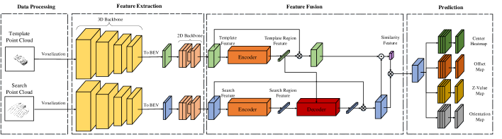
Figure 1: An overview of our LiDAR-based 3D Object Tracking with Transformer framework (LTTR). $\odot$ is the cross-correlation operation, $\otimes$ represents multiplication operation.

3 Method

In this section, we present the proposed framework, named LTTR. As shown in Figure 1, the framework consists of data processing, feature extraction, feature fusion, and prediction. We will introduce the details of LTTR in the following subsections.

3.1 Overall Architecture

Data Processing. We adopt the Siamese-like tracking pipeline which inputs template and search point cloud to top and bottom branches respectively. By reading the label, we obtain the 3D box of the target object and transform the whole scene point clouds into the local coordinate system whose origin is set as the center of the box. After that, we randomly shift the (x,y) of the center of the 3D box to get the training label value in the search branch, then normalize the points into the x-axis of the box in the template branch. Finally, we apply the same 3D range to both branches to get the input pair. The point cloud in the 3D range in the search branch is the search point cloud, and the point cloud in the 3D box in the template branch is the template point cloud. For both branches, we divide the points into regular voxels with a spatial resolution of $W\times L\times H$ and get input $\mathit{I}\in\mathbb{R}^{\mathit{W}\times\mathit{L}\times\mathit{H}}$.

Feature Extraction. We use the 3D sparse convolution network and 2D convolution network as the backbone network to extract features for both branches. Through 3D sparse convolution, the voxels are converted into feature volumes with $8\times$ downsampled sizes. By converting the $8\times$ downsampled 3D feature volumes into BEV representation, the final feature map $\mathit{M}\in\mathbb{R}^{\mathit{\frac{W}{8}}\times\mathit{\frac{L}{8}}\times\mathit{F}}$ is generated following the 2D backbone network, where $F$ is the feature channels. The weights are sharing between two branches.

Feature Fusion. Subsequently, we update and fuse the search feature $\mathit{M}_{s}$ and the template feature $\mathit{M}_{t}$ in the feature fusion network. As shown in Figure 1, $\mathit{M}_{s}$ and $\mathit{M}_{t}$ are first fed into the encoder respectively, and then sent into the decoder together. Following [Han et al.(2021)Han, Xiao, Wu, Guo, Xu, and Wang], the transformer encoder receives $\mathit{M}\in\mathbb{R}^{\mathit{\frac{W}{8}}\times\mathit{\frac{L}{8}}\times\mathit{F}}$ and outputs region feature $\mathit{G}\in\mathbb{R}^{\mathit{N}\times\mathit{D}}$ of channel $D$ with $N$ regions. The transformer decoder propagates information from template regions $\mathit{G}_{t}$ to search regions $\mathit{G}_{s}$ and decodes a fused $\mathit{G}_{s}\in\mathbb{R}^{\mathit{N}\times\mathit{D}}$ through cross-attention. Moreover, we project the region feature $\mathit{G}\in\mathbb{R}^{\mathit{N}\times\mathit{D}}$ to $\mathit{G}\in\mathbb{R}^{\mathit{N}\times\mathit{1}}$ as an attention weight by a fully-connected layer in both branches, and unfold the original feature $\mathit{M}$ to the size of ${\mathit{\frac{W\times L\times F}{64\times N}}\times\mathit{N}}$ to multiply with $\mathit{G}$. The feature is recovered back to the size of ${\frac{W}{8}}\times\mathit{\frac{L}{8}}\times\mathit{F}$ finally. The details of transformer architecture will be described in Section 3.2. Following the depthwise cross-correlation, the similarity feature with size ${\mathit{1}\times\mathit{1}\times\mathit{F}}$ is computed between $\mathit{M}_{s}$ and $\mathit{M}_{t}$. Finally, we multiply the similarity feature with $\mathit{M}_{s}$ to recover feature size for dense prediction.

Prediction. Following [Zhou et al.(2019)Zhou, Wang, and Krähenbühl, Ge et al.(2020)Ge, Ding, Hu, Wang, Chen, Huang, and Li], we use a center-based regression to predict several object properties. The regression consists of four heads, including the center heatmap head, local offset head, z-axis location head, and orientation head. Since our aim is to track the target object, we follow the assumption in [Qi et al.(2020)Qi, Feng, Cao, Zhao, and Xiao] that the 3D object size is known. The heads produce a center heatmap $\mathit{\hat{H}}\in\mathbb{R}^{\mathit{\frac{W}{8}}\times\mathit{\frac{L}{8}}\times\mathit{C}}$, a local offset regression map $\mathit{\hat{O}}\in\mathbb{R}^{\mathit{\frac{W}{8}}\times\mathit{\frac{L}{8}}\times\rm{2}}$, a z-value map $\mathit{\hat{Z}}\in\mathbb{R}^{\mathit{\frac{W}{8}}\times\mathit{\frac{L}{8}}\times\mathit{1}}$ and an orientation map $\hat{\Theta}\in\mathbb{R}^{\mathit{\frac{W}{8}}\times\mathit{\frac{L}{8}}\times\mathit{2}}$ respectively, where $\mathit{C}$ is the number of classes (1 in our tracking task) and orientation includes $sin(\theta)$ and $cos(\theta)$. We follow [Ge et al.(2020)Ge, Ding, Hu, Wang, Chen, Huang, and Li] to set heatmap value for every point $(x,y)$ in the downsampling feature map as:

$$H_{x,y,c}=\begin{cases}1,&\text{if $d=0$}\\ 0.8,&\text{if $d=1$}\\ \frac{1}{d},&\text{otherwise}\end{cases}$$ (1)

where $d$ is the Euclidean distance calculated between the object center and the point location in the downsample BEV map. A prediction $\mathit{\hat{H}_{x,y,c}=}$ $1$ corresponds to the object center and $\mathit{\hat{H}_{x,y,c}=}$ $0$ corresponds to background. We train the heatmap with focal loss [Lin et al.(2017)Lin, Goyal, Girshick, He, and Dollar]:

$$\mathcal{L}_{heat}=-\frac{1}{N}\sum_{x,y,c}\begin{cases}\left(1-\hat{H}_{x,y,c}\right)^{\alpha}\log\left(\hat{H}_{x,y,c}\right)\quad\smash{{\text{if ${H}_{x,y,c}=1$}}}\\ \left(1-H_{x,y,c}\right)^{\beta}\left(\hat{H}_{x,y,c}\right)^{\alpha}\quad\quad\ \smash{\raisebox{-6.88889pt}{\text{otherwise}}}\\ \quad\quad\log\left(1-\hat{H}_{x,y,c}\right),\\ \end{cases}$$ (2)

For other heads, we use L1 loss:

$$\mathit{\mathcal{L}_{v}}=\frac{1}{N}\sum_{k=1}^{N}\mathit{\left|\hat{V}_{p^{(k)}}-v^{(k)}\right|}.$$ (3)

where $\mathcal{L}_{v}\in(\mathcal{L}_{off},\mathcal{L}_{z},\mathcal{L}_{ori})$, $\hat{V}$ is the true value and $v^{(k)}$ is the predicted value for these heads. Therefore, the overall training loss is

$$\mathit{\mathcal{L}=\mathcal{L}_{heat}+\lambda_{off}\mathcal{L}_{off}+\lambda_{z}\mathcal{L}_{z}+\lambda_{ori}\mathcal{L}_{ori}}$$ (4)

where $\lambda$ is the regularization parameter for each head.

3.2 Transformer Architecture

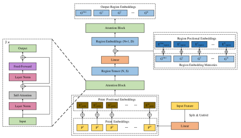
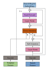
Figure 2: (a) The transformer encoder. (b)An overview of the proposed transformer architecture.

Multi-head Attention. Attention function is the core of the transformer, thus we first briefly review the principle of attention. Given query matrix $Q$, key matrix $K$ and value matrix $V$, attention function computes the similarity matrix between query and key, then multiplies value with normalized similarity, defined as:

$$\mathrm{Attention}(Q,K,V)=\mathrm{softmax}(\frac{QK^{T}}{\sqrt{d_{k}}})V$$ (5)

where $d_{k}$ is the dimension of key. Meanwhile, multiple heads are usually utilized in the attention function. Multi-head attention (MHA) projects query, key, and value into different feature spaces $h$ times, where $h$ is the number of heads, and computes the attention in parallel for every of these projected queries, keys, and values. The results from different heads are concatenated and projected to the final value. Following [Vaswani et al.(2017)Vaswani, Shazeer, Parmar, Uszkoreit, Jones, Gomez, Kaiser, and Polosukhin], the define of MHA is:

$$\mathrm{MHA}(Q,K,V)=\mathrm{Concat}(\mathrm{head_{1}},...,\mathrm{head_{h}})W^{O}$$ (6)

where $\mathrm{head_{i}}=\mathrm{Attention}(QW^{Q}_{i},KW^{K}_{i},VW^{V}_{i})$ and $W^{O}\in\mathbb{R}^{hd_{v}\times d_{model}}$, $d_{v}$ is the dimension of value and $d_{model}$ is the dimension of a single head attention.

Transformer Encoder. The transformer encoder takes BEV point cloud feature $\mathit{M}\in\mathbb{R}^{\mathit{\frac{W}{8}}\times\mathit{\frac{L}{8}}\times\mathit{F}}$ as its input. Following [Han et al.(2021)Han, Xiao, Wu, Guo, Xu, and Wang], we first split $M$ into $N$ non-overlapping regions of resolution $(R,R)$ and reshape them to $\mathit{M^{\prime}}\in\mathbb{R}^{\mathit{N}\times(\mathit{R}\times\mathit{R}\times\mathit{F})}$, where $\mathit{N}=\frac{W}{8R}\times\frac{L}{8R}$. Meanwhile, we also transform each region into the target size $(R^{\prime},R^{\prime})$ with point unfold. After applying a linear projection, the sequence of regions can be formed as:

$$\mathcal{U}_{0}=[U_{0}^{1},U_{0}^{2},\cdots,U_{0}^{N}]\in\mathbb{R}^{{N}\times(R^{\prime}\times R^{\prime}\times S)}$$ (7)

where $U_{0}^{i}\in\mathbb{R}^{R^{\prime}\times R^{\prime}\times S}$, $i=1,2,\cdots,N$, and $S$ is the number of channels. Furthermore, each region tensor can also be viewed as a sequence of point tensors:

$$U_{0}^{i}=[P_{0}^{i,1},P_{0}^{i,2},\cdots,P_{0}^{i,{N^{\prime}}}]$$ (8)

where $N^{\prime}=R^{\prime 2}$. By utilizing multi-head self-attention, we could explore the intra-relation among regions:

$$\hat{U_{j}^{i}}=U_{j-1}^{i}+\mathrm{MHA}(U_{j-1}^{i},U_{j-1}^{i},U_{j-1}^{i}),$$ (9)

$$U_{j}^{i}=\hat{U_{j}^{i}}+\mathrm{FFN}(\hat{U_{j}^{i}}).$$ (10)

where $j=1,2,\cdots,J$ is the index of the $j$-th layer, $J$ is the total number of layers, and FFN means the feed-forward network, which is a 2-layer MLP module. The point-level MHA builds the local relations among points within one region and produces the region tensor. Additionally, similar to previous vision transformer works [Dosovitskiy et al.(2020)Dosovitskiy, Beyer, Kolesnikov, Weissenborn, Zhai, Unterthiner, Dehghani, Minderer, Heigold, Gelly, Uszkoreit, and Houlsby, Han et al.(2021)Han, Xiao, Wu, Guo, Xu, and Wang, Carion et al.(2020)Carion, Massa, Synnaeve, Usunier, Kirillov, and Zagoruyko], we create a set of learnable parameters called region embedding memories $\mathcal{G}_{0}$ for the region tensors and take them into output as the region representations. Specially, the region embedding memories are added with the region tensors in each layer:

$$\mathcal{G}_{0} =[G_{\text{class}},G_{0}^{1},G_{0}^{2},\cdots,G_{0}^{N}]\in\mathbb{R}^{(N+1)\times D}$$ (11)

$$G_{j-1}^{i} =G_{j-1}^{i}+\mathrm{\Phi}(U_{j-1}^{i}),$$ (12)

where $G_{\text{class}}$ is the global point cloud embedding, $G_{j-1}^{i}\in\mathbb{R}^{D}$, $\Phi$ is the projection function, which is fully-connected layer in our implementation. We random initialize all of the region embedding memories. Meanwhile, we utilize the MHA once again for region embeddings. The mechanism can be summarized as:

$$\hat{{G}_{j}^{i}} ={G}_{j-1}^{i}+\mathrm{MHA}({G}_{j-1}^{i},{G}_{j-1}^{i},{G}_{l-1}^{i}),$$ (13)

$${G}_{j}^{i} =\hat{{G}_{j}^{i}}+\mathrm{FFN}(\hat{{G}_{j}^{i}}).$$ (14)

The region-level MHA explores the inter-relation among regions, building the global information of the point cloud. Therefore, the region embedding memories learn the region representation by adding to region tensors and being sent into the MHA during training. Meanwhile, although $G_{\text{class}}$ does not have a corresponding region tensor to add, it can also capture the global information by exchanging information with the other region embeddings through the region-level MHA. Furthermore, we use standard learnable 1D position embeddings to add to embeddings as follows:

$$T=T+E$$ (15)

where $T\in(G,U)$, $E\in(E_{region},E_{point})$, $E_{region}\in\mathbb{R}^{(N+1)\times D}$ and $E_{point}\in\mathbb{R}^{N^{\prime}\times S}$. Both the region and point position embeddings are added to the corresponding embeddings before MHA and are shared across the same data level, thus the local and global spatial information can be maintained. The whole process is shown in Figure 2.

By processing both points and regions, the encoder explores the local information across points within regions and global relations across regions, producing $\mathit{G}\in\mathbb{R}^{(\mathit{N}+1)\times\mathit{D}}$for each point cloud feature $\mathit{M}$. We take $G=[G_{0}^{1},G_{0}^{2},\cdots,G_{0}^{N}]\in\mathbb{R}^{N\times D}$ as the input of the decoder.

Transformer Decoder. The above encoder processes template and search features separately, thus the information only flows within the point cloud itself. To build the inter-relation between point clouds and exchange information across branches, we further utilize a transformer decoder to fuse features. The decoder fuses features by propagating template region feature $\mathit{G}_{t}$ to search region feature $\mathit{G}_{s}$. The decoder first updates the search region feature $\mathit{G}_{s}$ by self-attention mechanism, then computes the similarity among regions from search and template point clouds based on the cross-attention mechanism. Specially, the decoder takes $\mathit{G}_{s}$ as the query and $\mathit{G}_{t}$ as key and value through the cross-attention, the fused search region feature $\mathit{G}_{s}$ is generated following a feed-forward layer. The decoder is shown in Figure 2 and can be summarized as:

$$\hat{G_{s}}=G_{s}+\mathrm{MHA}(G_{s},G_{s},G_{s}),$$ (16)

$$\tilde{G_{s}}=\hat{G_{s}}+\mathrm{MHA}(\hat{G_{s}},G_{t},G_{t}),$$ (17)

$$G_{s}=\tilde{G_{s}}+\mathrm{FFN}(\tilde{G_{s}}).$$ (18)

Through the decoder, the search and template region features exchange region information, which makes the search region feature include much more information of the target object and computes the region attention. To have clear representations, the layer norm operation is not represented in the above equations.

4 Experiments

4.1 Datasets and Evaluation

We use KITTI tracking dataset [Geiger et al.(2012)Geiger, Lenz, and Urtasun] as the benchmark and follow [Qi et al.(2020)Qi, Feng, Cao, Zhao, and Xiao] in data split. We also use One Pass Evaluation (OPE) as evaluation metric, including Success and Precision.

4.2 Implementation Details

In data processing, we set point cloud range as [-3.2m, 3.2m], [-3.2m, 3.2m], [-3m, 1m] along x, y, z axis, and set voxel size as [0.025m, 0.025m, 0.05m]. The template and search points are voxelized following [Zhou and Tuzel(2018)]. A maximum of five points are randomly sampled from each voxel. Meanwhile, we use the same backbone as  [Zhou and Tuzel(2018), Yan et al.(2018)Yan, Mao, and Li]. In regression, each head consists of four convolution layers to predict and the heatmap head is followed by a sigmoid function to generate the final score. Following the training setting of the popular codebase OpenPCDet [Team(2020)], we train the network end-to-end with 80 epochs and 36 batch. In loss setting, we set $\alpha=2$, $\beta=4$ in Equation 2, and set $\lambda_{z}=1.5$, $\lambda_{off}=\lambda_{ori}=1$ in Equation 4.

Method Reference LiDAR RGB Success Precision FPS SC3D [Giancola et al.(2019)Giancola, Zarzar, and Ghanem] CVPR2019 $\surd$ 41.3 57.9 1.8 F-Siamese [Zou et al.(2020)Zou, Cui, Kong, Zhang, Liu, Wen, and Li] IROS2020 $\surd$ $\surd$ 37.1 50.6 - P2B [Qi et al.(2020)Qi, Feng, Cao, Zhao, and Xiao] CVPR2020 $\surd$ 56.2 72.8 45.5 LTTR(Ours) - $\surd$ 65.0 77.1 22.6

Table 1: Comprehensive comparison with state-of-the-art trackers on Car category.

Method Car Pedestrian Van Cyclist Mean Frame Number 6424 6088 1248 308 14068 Success SC3D [Giancola et al.(2019)Giancola, Zarzar, and Ghanem] 41.3 18.2 40.4 41.5 31.2 F-Siamese [Zou et al.(2020)Zou, Cui, Kong, Zhang, Liu, Wen, and Li] 37.1 16.2 - 47.0 - P2B [Qi et al.(2020)Qi, Feng, Cao, Zhao, and Xiao] 56.2 28.7 40.8 32.1 42.4 LTTR(Ours) 65.0 33.2 35.8 66.2 48.7 Precision SC3D [Giancola et al.(2019)Giancola, Zarzar, and Ghanem] 57.9 37.8 47.0 70.4 48.5 F-Siamese [Zou et al.(2020)Zou, Cui, Kong, Zhang, Liu, Wen, and Li] 50.6 32.2 - 77.2 - P2B [Qi et al.(2020)Qi, Feng, Cao, Zhao, and Xiao] 72.8 49.6 48.4 44.7 60.0 LTTR(Ours) 77.1 56.8 45.6 89.9 65.8

Table 2: Extensive comparisons with state-of-the-art trackers on multiple categories.

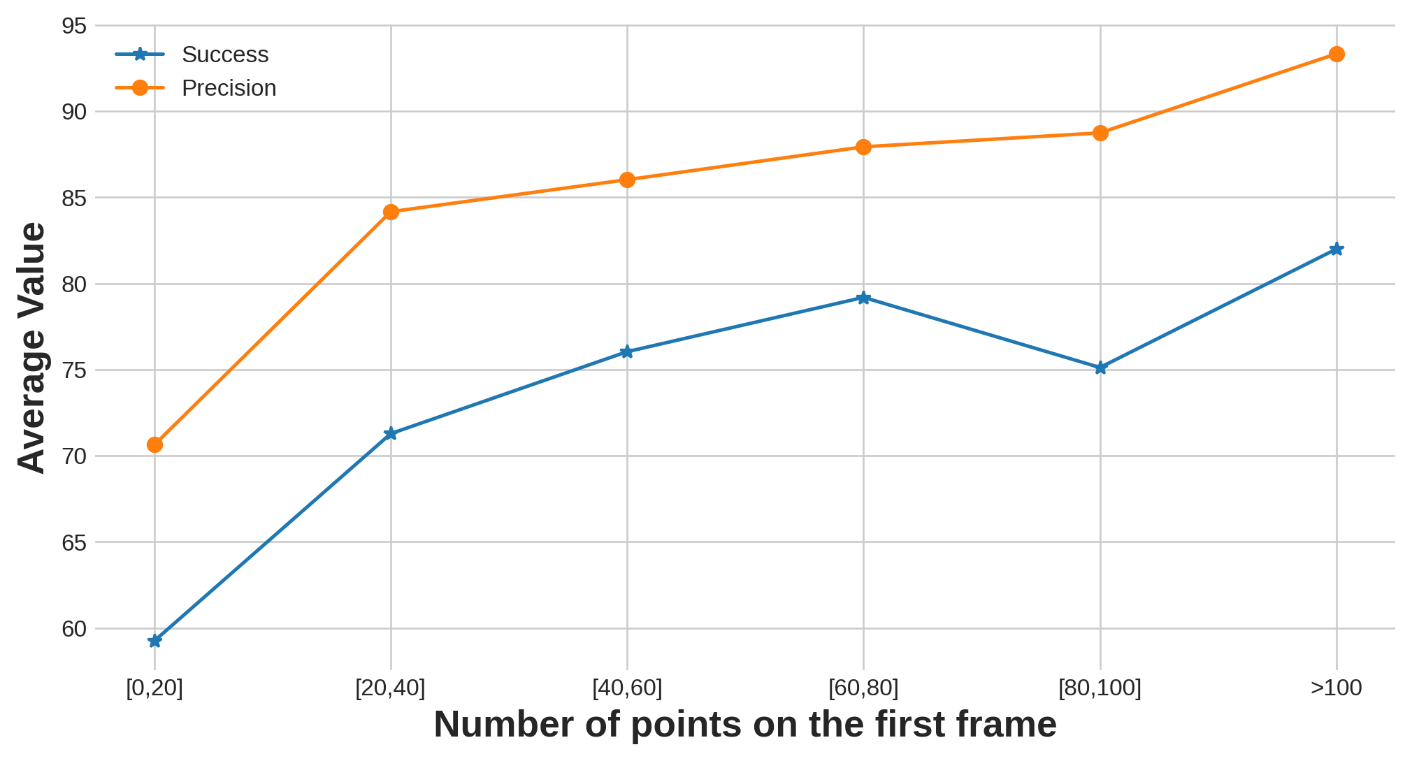
Figure 3: The influence of the number of points on the first frame car.

4.3 State-of-the-art Comparisons

We compare our LTTR with previous state-of-the-art methods on KITTI dataset. As shown in Table 1, our approach surpasses the previous methods by +8.8% Success and +4.3% Precision respectively in the Car category. Additionally, LTTR achieves a real-time running speed. We also report multiple categories tracking results on KITTI dataset, including Pedestrian, Van, and Cyclist. As shown in Table 2, our method outperforms P2B [Qi et al.(2020)Qi, Feng, Cao, Zhao, and Xiao] by 5% on average. In particular, LTTR shows its advantages on objects with a small size, e.g. Pedestrian and Cyclist, surpassing previous methods by a large margin. Considering the difference among these categories, our method is a general and efficient method for different categories.

We also report the influence of the number of the first frame point in the Car category. As shown in Figure 3, with more points, LTTR has a higher performance. We believe that more points in the first frame give the network enough information about the target to track.

Different Network Version	Success	Precision
Baseline	57.2	70.9
Encoder (w/o Decoder)	${\text{60.6}}_{3.4\%\uparrow}$	${\text{71.9}}_{1.0\%\uparrow}$
Encoder + Decoder (Max)	${\text{64.2}}_{7.0\%\uparrow}$	$\textbf{77.3}_{6.4\%\uparrow}$
Encoder + Decoder	$\textbf{65.0}_{7.8\%\uparrow}$	$\text{77.1}_{6.2\%\uparrow}$

Table 3: Ablative study of our transformer architecture.

4.4 Ablation Study

In this section, we ablate the proposed method on the Car category of KITTI dataset. We first ablate the transformer network to verify the influence of the encoder and decoder. We introduce a baseline version and a Max-Decoder version. The baseline version does not have any transformer component, and the Max-Decoder version inputs $\mathit{G}_{class}$ instead of $G=[G_{0}^{1},G_{0}^{2},\cdots,G_{0}^{N}]$ in the template branch to the decoder. Moreover, we compare the different numbers of heads, layers and region sizes in the transformer to validate our design choices. Finally, we compare different backbones and regression heads to explore their influence on the proposed method.

Effect of Encoder. As shown in Table 3, with the transformer encoder, the performance has +3.4% and +1.0% gains on Success and Precision respectively. The result indicates the effectiveness of our encoder to build the local and global relations of point cloud. It is worth noting that even without any transformer component, our baseline version has a competitive performance with the state-of-the-art methods.

Effect of Decoder. We further add the transformer decoder. Specially, we evaluate two decoder versions different in template input. As shown in Table 3, both of them bring significant performance improvements. However, compared to Max-version, our version has a balanced result between Success and Precision. We believe that the Max-version loses the inter-relation among regions of the point cloud due to its single global input.

		Success	Precision
Head Number	1	61.0	73.7
	2	61.6	74.6
	4	62.1	75.3
	8	65.0	77.1
	12	63.8	78.3
Layer Number	1	65.0	77.1
	2	61.9	74.3
	4	62.7	75.7
	6	61.1	73.8
	8	60.2	73.2
Region Size	1	60.5	73.3
	4	63.6	76.7
	16	65.0	77.1

Table 4: Ablative study of our transformer architecture.

Structure Modifications. We also discuss the details of our transformer structure as shown in Table 4, including the number of heads, number of encoder/decoder layers and the region size. All experimental networks have a complete encoder and decoder component. For the number of heads, we observe that heads=8 achieves the best performance, while increase heads to 12 results in a decrease in Success but an increase in Precision. The results indicate that MHA is efficient in our transformer architecture, as discussed in Section 3.2, but too many heads may result in degeneration in orientation prediction. Meanwhile, stacking more layers does not bring in performance improvement but has more parameters and lower speed. We speculate that more layers may divide the template and search features into different feature subspaces. Different from detection task, the tracking task has two input branches and tracks the object based on their similarity. Therefore, tracking method requires the template and search features to be in the same feature spaces to have a better similarity computation. Additionally, with a small region size, the performance of the network degenerates to the encoder version. We believe that the smaller size generates more regions and leads to the decoder not being able to exchange global information effectively. Thus, we use the max non-overlapping size $R=16$ for higher performance.

Backbone. We also make modifications to the backbone to explore whether the performance could be further improved by increasing the parameters in the backbone. Our backbone follows Second [Yan et al.(2018)Yan, Mao, and Li], a backbone baseline in 3D vision for its simple architecture and wide use [Shi et al.(2020)Shi, Guo, Jiang, Wang, Shi, Wang, and Li, Zhou and Tuzel(2018), Chen et al.(2019)Chen, Liu, Shen, and Jia]. The baseline includes 3D and 2D backbones to process voxels and BEV features respectively. The 3D backbone is termed as BaseVoxel and the 2D backbone is termed as BaseBEV. In this comparison experiment, we use the resnet-manner version of BaseVoxel in OpenPCDet [Team(2020)] and termed it as ResVoxel, which adds a residual path in every sparse block of BaseVoxel. Meanwhile, we add one convolution block to BaseBEV and term it as DeepBEV. Therefore, the ResVoxel has more parameters than BaseVoxel, and DeepBEV is deeper than BaseBEV. However, as Table 5 shows, with the network going deeper and the total parameters becoming larger, the performance does not have improved but decreased. We speculate that more parameters in the backbone may hinder the transformer to capture useful information, thus our baseline backbone could achieve better performance with fewer parameters comparing to these modifications.

3D Backbone	2D Backbone	3D Params	2D Params	Success	Precision
BaseVoxel	BaseBEV	1.280K	8.266M	65.0	77.1
	DeepBEV	1.280K	12.988M	62.4	76.4
ResVoxel	BaseBEV	2.656K	8.266M	62.6	75.4
	DeepBEV	2.656K	12.988M	60.2	73.8

Table 5: Ablative study of different 3D and 2D backbones.

Regression Head. We compare our center-based regression head with an anchor-based counterpart. For anchor-based regression, we follow the setting of Second [Yan et al.(2018)Yan, Mao, and Li]. Specially, for every location, we set two anchors with 0 degrees and 90 degrees, and the thresholds for

	Success	Precision
Center-based	65.0	77.1
Anchor-based	65.3	75.1

Table 6: Comparison of different regression heads.

positive and negative are 0.6 and 0.45 respectively. As shown in Table 6, the anchor-based regression improves the Success 0.3 points while reduces the Precision 2.0 points. The result shows that the center-based regression has better prediction results in location but is weaker in rotation regression compared to anchor-based regression. We believe this is because of the pre-defined anchor rotation degree in anchor-based regression. Meanwhile, the anchor-based regression needs more hyper-parameters in the anchor setting which needs fine-tuning. Therefore, to have fewer hyper-parameters and more balanced tracking results, we adopt the center-based regression.

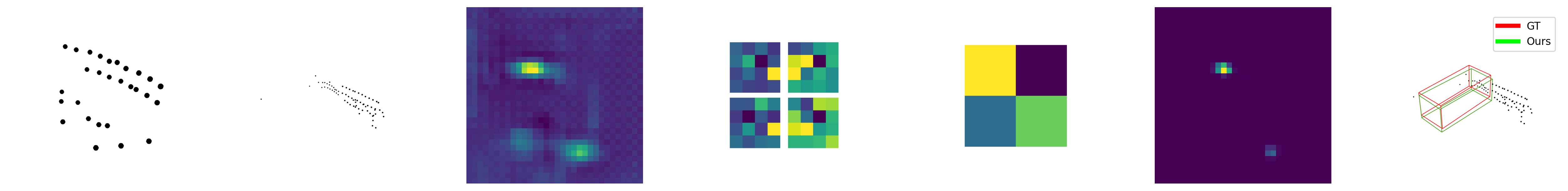
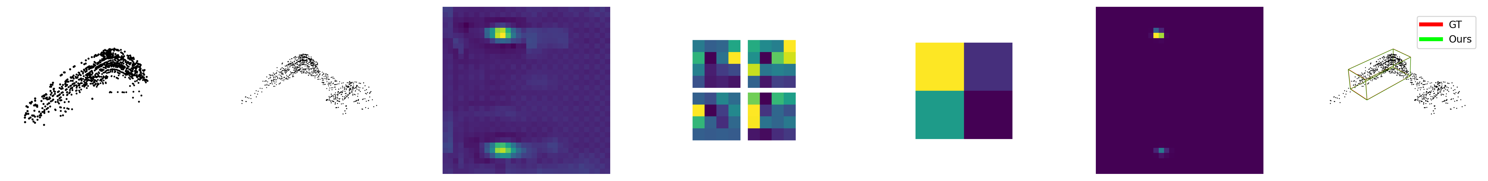
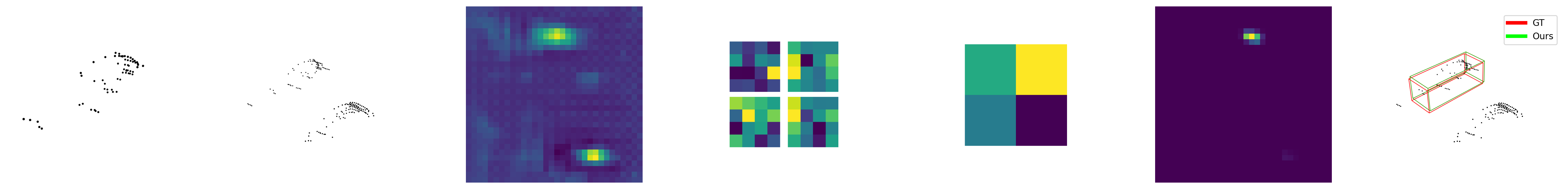
Figure 4: Visualization results. There are template point cloud, search point cloud, heatmap without transformer, point-level attention, region-level attention, heatmap with transformer and the predicted boxes from left to right.

4.5 Qualitative Visualization

To explore the effect of the transformer network, we visualized the predicted heatmap and the transformer point and region weights, as shown in Figure 4. Compared to the heatmap without transformer, the heatmap with transformer accurately finds the target position with the help of point and region attentions, avoiding the false track. The results verify the effectiveness of the proposed transformer network, even for target object with sparse points.

5 Conclusions

In this paper, we present LTTR, a novel tracking framework based on the transformer. Through the transformer network, LTTR builds local information and global relation within the point cloud, explores the inter-relation between point clouds, and predicts the 3D bounding box of the target object by a center-based regression. Comprehensive experiments on KITTI dataset demonstrate that our method achieves new state-of-the-art performance. In the future, we will investigate how to integrate temporal information into our method.

Acknowledgments This work was supported by National Natural Science Foundation of China (62073066, U20A20197), Science and Technology on Near-Surface Detection Laboratory (6142414200208), the Fundamental Research Funds for the Central Universities (N182608003), Major Special Science and Technology Project of Liaoning Province (No.2019JH1/10100026), and Aeronautical Science Foundation of China (No.201941050001).

References

- [Bertinetto et al.(2016)Bertinetto, Valmadre, Henriques, Vedaldi, and Torr] Luca Bertinetto, Jack Valmadre, João F. Henriques, Andrea Vedaldi, and Philip H. S. Torr. Fully-convolutional siamese networks for object tracking. In Computer Vision – ECCV 2016 Workshops, pages 850–865, Cham, 2016. Springer International Publishing. ISBN 978-3-319-48881-3.
- [Bibi et al.(2016)Bibi, Zhang, and Ghanem] Adel Bibi, Tianzhu Zhang, and Bernard Ghanem. 3d part-based sparse tracker with automatic synchronization and registration. In 2016 IEEE Conference on Computer Vision and Pattern Recognition (CVPR), pages 1439–1448, 2016. 10.1109/CVPR.2016.160.
- [Carion et al.(2020)Carion, Massa, Synnaeve, Usunier, Kirillov, and Zagoruyko] Nicolas Carion, Francisco Massa, Gabriel Synnaeve, Nicolas Usunier, Alexander Kirillov, and Sergey Zagoruyko. End-to-end object detection with transformers. In Computer Vision – ECCV 2020, pages 213–229, Cham, 2020. Springer International Publishing. ISBN 978-3-030-58452-8.
- [Chen et al.(2021)Chen, Yan, Zhu, Wang, Yang, and Lu] Xin Chen, Bin Yan, Jiawen Zhu, Dong Wang, Xiaoyun Yang, and Huchuan Lu. Transformer tracking. 2021. URL https://arxiv.org/abs/2103.15436.
- [Chen et al.(2019)Chen, Liu, Shen, and Jia] Yilun Chen, Shu Liu, Xiaoyong Shen, and Jiaya Jia. Fast point r-cnn. In Proceedings of the IEEE/CVF International Conference on Computer Vision (ICCV), October 2019.
- [Chu et al.(2021)Chu, Tian, Zhang, Wang, Wei, Xia, and Shen] Xiangxiang Chu, Zhi Tian, Bo Zhang, Xinlong Wang, Xiaolin Wei, Huaxia Xia, and Chunhua Shen. Conditional positional encodings for vision transformers. 2021. URL https://arxiv.org/abs/2102.10882.
- [Danelljan et al.(2019)Danelljan, Bhat, Khan, and Felsberg] Martin Danelljan, Goutam Bhat, Fahad Shahbaz Khan, and Michael Felsberg. Atom: Accurate tracking by overlap maximization. In 2019 IEEE/CVF Conference on Computer Vision and Pattern Recognition (CVPR), pages 4655–4664, 2019. 10.1109/CVPR.2019.00479.
- [Dosovitskiy et al.(2020)Dosovitskiy, Beyer, Kolesnikov, Weissenborn, Zhai, Unterthiner, Dehghani, Minderer, Heigold, Gelly, Uszkoreit, and Houlsby] Alexey Dosovitskiy, Lucas Beyer, Alexander Kolesnikov, Dirk Weissenborn, Xiaohua Zhai, Thomas Unterthiner, Mostafa Dehghani, Matthias Minderer, Georg Heigold, Sylvain Gelly, Jakob Uszkoreit, and Neil Houlsby. An image is worth 16x16 words: Transformers for image recognition at scale. 2020. URL https://arxiv.org/abs/2010.11929.
- [Ge et al.(2020)Ge, Ding, Hu, Wang, Chen, Huang, and Li] Runzhou Ge, Zhuangzhuang Ding, Yihan Hu, Yu Wang, Sijia Chen, Li Huang, and Yuan Li. Afdet: Anchor free one stage 3d object detection. 2020. URL https://arxiv.org/abs/2006.12671.
- [Geiger et al.(2012)Geiger, Lenz, and Urtasun] Andreas Geiger, Philip Lenz, and Raquel Urtasun. Are we ready for autonomous driving? the kitti vision benchmark suite. In 2012 IEEE Conference on Computer Vision and Pattern Recognition (CVPR), pages 3354–3361, 2012. 10.1109/CVPR.2012.6248074.
- [Giancola et al.(2019)Giancola, Zarzar, and Ghanem] Silvio Giancola, Jesus Zarzar, and Bernard Ghanem. Leveraging shape completion for 3d siamese tracking. In Proceedings of the IEEE/CVF Conference on Computer Vision and Pattern Recognition (CVPR). IEEE, June 2019. ISBN 9781728132938. 10.1109/cvpr.2019.00145. URL http://dx.doi.org/10.1109/CVPR.2019.00145.
- [Han et al.(2021)Han, Xiao, Wu, Guo, Xu, and Wang] Kai Han, An Xiao, Enhua Wu, Jianyuan Guo, Chunjing Xu, and Yunhe Wang. Transformer in transformer. 2021. URL https://arxiv.org/abs/2103.00112.
- [Held et al.(2016)Held, Thrun, and Savarese] David Held, Sebastian Thrun, and Silvio Savarese. Learning to track at 100 fps with deep regression networks. In Computer Vision – ECCV 2016, pages 749–765, Cham, 2016. Springer International Publishing. ISBN 978-3-319-46448-0.
- [Kart et al.(2019)Kart, Kämäräinen, and Matas] Uğur Kart, Joni-Kristian Kämäräinen, and Jiří Matas. How to make an rgbd tracker? In Computer Vision – ECCV 2018 Workshops, pages 148–161, Cham, 2019. Springer International Publishing. ISBN 978-3-030-11009-3.
- [Li et al.(2018)Li, Yan, Wu, Zhu, and Hu] Bo Li, Junjie Yan, Wei Wu, Zheng Zhu, and Xiaolin Hu. High performance visual tracking with siamese region proposal network. In 2018 IEEE/CVF Conference on Computer Vision and Pattern Recognition (CVPR), pages 8971–8980, 2018. 10.1109/CVPR.2018.00935.
- [Li et al.(2019)Li, Wu, Wang, Zhang, Xing, and Yan] Bo Li, Wei Wu, Qiang Wang, Fangyi Zhang, Junliang Xing, and Junjie Yan. Siamrpn++: Evolution of siamese visual tracking with very deep networks. In 2019 IEEE/CVF Conference on Computer Vision and Pattern Recognition (CVPR), pages 4277–4286, 2019. 10.1109/CVPR.2019.00441.
- [Lin et al.(2017)Lin, Goyal, Girshick, He, and Dollar] Tsung-Yi Lin, Priya Goyal, Ross Girshick, Kaiming He, and Piotr Dollar. Focal loss for dense object detection. In 2017 IEEE International Conference on Computer Vision (ICCV). IEEE, Oct 2017. ISBN 9781538610329. 10.1109/iccv.2017.324. URL http://dx.doi.org/10.1109/iccv.2017.324.
- [Liu et al.(2021)Liu, Lin, Cao, Hu, Wei, Zhang, Lin, and Guo] Ze Liu, Yutong Lin, Yue Cao, Han Hu, Yixuan Wei, Zheng Zhang, Stephen Lin, and Baining Guo. Swin transformer: Hierarchical vision transformer using shifted windows, 2021. URL https://arxiv.org/abs/2103.14030.
- [Meinhardt et al.(2021)Meinhardt, Kirillov, Leal-Taixe, and Feichtenhofer] Tim Meinhardt, Alexander Kirillov, Laura Leal-Taixe, and Christoph Feichtenhofer. Trackformer: Multi-object tracking with transformers. 2021. URL https://arxiv.org/abs/2101.02702.
- [Qi et al.(2020)Qi, Feng, Cao, Zhao, and Xiao] Haozhe Qi, Chen Feng, Zhiguo Cao, Feng Zhao, and Yang Xiao. P2b: Point-to-box network for 3d object tracking in point clouds. In 2020 IEEE/CVF Conference on Computer Vision and Pattern Recognition (CVPR). IEEE, Jun 2020. ISBN 9781728171685. 10.1109/cvpr42600.2020.00636. URL http://dx.doi.org/10.1109/CVPR42600.2020.00636.
- [Shi et al.(2020)Shi, Guo, Jiang, Wang, Shi, Wang, and Li] Shaoshuai Shi, Chaoxu Guo, Li Jiang, Zhe Wang, Jianping Shi, Xiaogang Wang, and Hongsheng Li. Pv-rcnn: Point-voxel feature set abstraction for 3d object detection. In IEEE/CVF Conference on Computer Vision and Pattern Recognition (CVPR), June 2020.
- [Sun et al.(2020)Sun, Jiang, Zhang, Xie, Cao, Hu, Kong, Yuan, Wang, and Luo] Peize Sun, Yi Jiang, Rufeng Zhang, Enze Xie, Jinkun Cao, Xinting Hu, Tao Kong, Zehuan Yuan, Changhu Wang, and Ping Luo. Transtrack: Multiple-object tracking with transformer. 2020. URL https://arxiv.org/abs/2012.15460.
- [Team(2020)] OpenPCDet Development Team. Openpcdet: An open-source toolbox for 3d object detection from point clouds. https://github.com/open-mmlab/OpenPCDet, 2020.
- [Vaswani et al.(2017)Vaswani, Shazeer, Parmar, Uszkoreit, Jones, Gomez, Kaiser, and Polosukhin] Ashish Vaswani, Noam Shazeer, Niki Parmar, Jakob Uszkoreit, Llion Jones, Aidan N Gomez, Ł ukasz Kaiser, and Illia Polosukhin. Attention is all you need. In Advances in Neural Information Processing Systems, volume 30. Curran Associates, Inc., 2017. URL https://proceedings.neurips.cc/paper/2017/file/3f5ee243547dee91fbd053c1c4a845aa-Paper.pdf.
- [Wang et al.(2021)Wang, Zhou, Wang, and Li] Ning Wang, Wengang Zhou, Jie Wang, and Houqaing Li. Transformer meets tracker: Exploiting temporal context for robust visual tracking. 2021. URL https://arxiv.org/abs/2103.11681.
- [Yan et al.(2018)Yan, Mao, and Li] Yan Yan, Yuxing Mao, and Bo Li. Second: Sparsely embedded convolutional detection. In Sensors, volume 18, 2018. 10.3390/s18103337. URL https://www.mdpi.com/1424-8220/18/10/3337.
- [Zhou et al.(2019)Zhou, Wang, and Krähenbühl] Xingyi Zhou, Dequan Wang, and Philipp Krähenbühl. Objects as points. 2019. URL https://arxiv.org/abs/1904.07850.
- [Zhou and Tuzel(2018)] Yin Zhou and Oncel Tuzel. Voxelnet: End-to-end learning for point cloud based 3d object detection. In 2018 IEEE/CVF Conference on Computer Vision and Pattern Recognition (CVPR). IEEE, Jun 2018. ISBN 9781538664209. 10.1109/cvpr.2018.00472. URL http://dx.doi.org/10.1109/CVPR.2018.00472.
- [Zhu et al.(2021)Zhu, Su, Lu, Li, Wang, and Dai] Xizhou Zhu, Weijie Su, Lewei Lu, Bin Li, Xiaogang Wang, and Jifeng Dai. Deformable detr: Deformable transformers for end-to-end object detection. In International Conference on Learning Representations (ICLR), 2021. URL https://openreview.net/forum?id=gZ9hCDWe6ke.
- [Zou et al.(2020)Zou, Cui, Kong, Zhang, Liu, Wen, and Li] Hao Zou, Jinhao Cui, Xin Kong, Chujuan Zhang, Yong Liu, Feng Wen, and Wanlong Li. F-siamese tracker: A frustum-based double siamese network for 3d single object tracking. In 2020 IEEE/RSJ International Conference on Intelligent Robots and Systems (IROS). IEEE, Oct 2020. ISBN 9781728162126. 10.1109/iros45743.2020.9341120. URL http://dx.doi.org/10.1109/IROS45743.2020.9341120.