Graphene as a source of entangled plasmons

Abstract

We analyze nonlinear optics schemes for generating pairs of quantum entangled plasmons in the terahertz-infrared range in graphene. We predict that high plasmonic field concentration and strong optical nonlinearity of monolayer graphene enables pair-generation rates much higher than those of conventional photonic sources. The first scheme we study is spontaneous parametric down conversion in a graphene nanoribbon. In this second-order nonlinear process a plasmon excited by an external pump splits into a pair of plasmons, of half the original frequency each, emitted in opposite directions. The conversion is activated by applying a dc electric field that induces a density gradient or a current across the ribbon. Another scheme is degenerate four-wave mixing where the counter-propagating plasmons are emitted at the pump frequency. This third-order nonlinear process does not require a symmetry-breaking dc field. We suggest nano-optical experiments for measuring position-momentum entanglement of the emitted plasmon pairs. We estimate the critical pump fields at which the plasmon generation rates exceed their dissipation, leading to parametric instabilities.

I Introduction

Graphene plasmonics has emerged as a platform for realizing strong light-matter interaction on ultrasmall length scales [1, 2]. Launching, detection, and manipulation of plasmons by near-field probes has been demonstrated at infrared/THz frequencies [3, 4, 5, 6, 7, 8, 9, 10, 11, 12, 13, 14]. High concentration of electric field, a key factor for nonlinear optical phenomena, has been achieved by exciting plasmons of wavelength $\lambda_{p}$ as small as few hundred nanometers, about two orders of magnitude shorter than the vacuum photon wavelength $\lambda_{v}$. Plasmonic quality factors up to $Q\sim 130$ have been reached [9] in encapsulated graphene structures [5, 7], fulfilling another condition — low dissipation — necessary for prominent nonlinear effects.

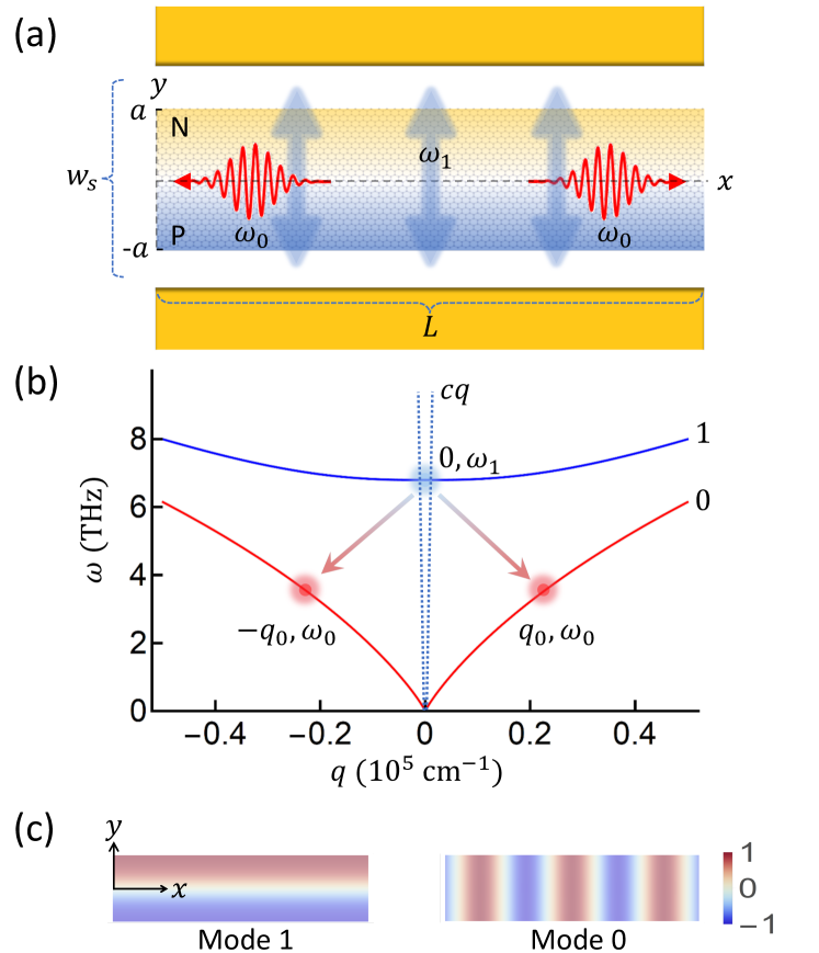
Figure 1: (Color online) (a) Type-A device: a graphene ribbon with a lateral p-n junction (blue/gold denoting electron/hole doping) induced by a split gate (golden bars). A pump field of frequency $\omega_{1}$ applied in the $\hat{\mathbf{y}}$-direction (thick arrows) generates plasmon pairs of frequency $\omega_{0}$ propagating in the $\pm\hat{\mathbf{x}}$ direction (red undulating arrows). (b) Plasmon dispersion in a ribbon of half-width $a=200\,\mathrm{nm}$ with the p-n junction on the midline and the carrier density $n=\pm 10^{12}\,\mathrm{cm^{-2}}$ at the edges. The dotted lines form the ‘light cone’ for the dispersion of vacuum photons. The blue dot represents the mode-$1$ plasmon pumped by the incident photon, which then decays into two mode-$0$ plasmons (the two red dots) as shown by the arrows. (c) The spatial distribution of the amplitude of the quasi-static electric potential of the two modes.

Numerous theoretical [15, 16, 17, 18, 19, 20, 21, 22, 23, 24] and a few experimental [25, 26] works have explored manifestations of nonlinear coupling of light to graphene in the context of conventional far-field optics. However, both nonlinear [27, 28, 29, 30, 23] and quantum [31, 28, 32] effects could be more pronounced in the near-field domain because of plasmonic field concentration. Plasmon interaction phenomena we study in this paper include the parametric down conversion (PDC) and four-wave mixing (FWM) [33]. Spontaneous PDC and FWM can generate entangled pairs of plasmons, similar to how the usual photonic spontanenous PDC produces entangled pairs of photons [34, 35, 36, 37, 38, 39, 40, 41].

We propose that a graphene ribbon containing an electrostatically induced p-n junction [42, 43, 5, 44, 45, 46], see Fig. 1(a), can be a highly efficient PDC source. The plasmon spectrum of such a system, which we will call the device of type A, consists of multiple continuously dispersing subbands. The lowest subband (labeled “$0$”) is gapless and the next one (labeled “$1$”) is gapped due to transverse confinement in the ribbon, see Fig. 1(b). In the simplest picture, the PDC process is splitting of a mode-$1$ plasmon of frequency $\omega_{1}$ and momentum $q_{1}=0$ into two mode-$0$ plasmons of frequency $\omega_{0}=\omega_{1}/2$ and momenta $\pm q_{0}$ that propagate away in opposite directions along the ribbon. The energy-momentum conservation (phase matching) in this conversion is guaranteed without any fine-tuning of the device. This advantage of the counterpropagating PDC scheme has been previously exploited in photonic waveguides [47, 39, 36, 48]. In a more precise description, frequencies $\omega_{0}$ and so the momenta $q$ of the outgoing plasmons have some uncertainty. The spontanenous PDC generates a superposition of states of different momentum:

$$|\psi\rangle=\int dqf(q)\,|{-q}\rangle\,|{+q}\rangle$$ (1)

where $|{-q}\rangle\,|{+q}\rangle$ means a two plasmon state with one plasmon at momentum $-q$ and the other at $+q$, see Sec. II.4. This superposition is not factorizable, which implies that the pairs are position-momentum entangled, similar to particles in the original Einstein, Podolsky, and Rosen (EPR) paper [34]. The amplitude function $f(q)$ in Eq. (1) is peaked at $q_{0}$ and has a characteristic width $\delta q\sim\gamma/v_{0}$ where

$$\gamma=\omega_{0}/Q$$ (2)

is the plasmon damping rate [9] and $v_{0}=d\omega_{0}/dq_{0}$ is the mode-$0$ plasmon group velocity.

The role of the split-gate represented by the golden bars in Fig. 1(a) is two-fold. First, it induces a gradient of carrier concentration in graphene when a dc voltage is applied between the two parts of the gate. The p-n junction is created when this voltage is high enough [44]. Such a system lacks inversion symmetry and therefore the PDC is allowed. Second, the split-gate serves as an optical antenna amplifying the incident pump field [44, 49] that excites mode-$1$ plasmons. The coupling is facilitated by a large transverse dipole moment of the mode-$1$ plasmons and a strong field enhancement $\lambda_{v}/\lambda_{p}\gg 1$ of the antenna.

Note that the inversion symmetry can also be broken by a dc current across a uniformly doped ribbon, which we refer to as the device of type B. In contrast, the FWM is a third-order nonlinear effect which does not require symmetry breaking fields. The degenerate FWM, in which the two pump photons of frequency $\omega$ are converted into a pair entangled plasmons of the same frequency, can take place in either a nanoribbon or a more typical larger-area graphene sheet, which are devices of type C.

Plasmonic effects similar to those we explore here have been considered in a few recent theoretical papers. For example, plasmonic sum-frequency generation in graphene nanoflakes [17] is based on the nonlinear mechanism similar to that underlying our plasmonic PDC. However, since the plasmon spectrum of a flake is discrete, only flakes of certain shapes can fulfill the energy-momentum conservation constraint for the sum (or difference) frequency generation. As mentioned above, in a long ribbon such kinematic constraints can be met without delicate fine-tuning. Another related work studied photon-plasmon difference frequency generation [26, 50] and entanglement [51], which is a phenomenon intermediate between the usual all-photon PDC [34] and our fully plasmonic PDC.

The remainder of the paper is organized as follows. In Sec. II, we summarize our main results for the type-A device. In the last part of that section we discuss possible experiments that can probe the plasmon entanglement. In Sec. III we consider the third-order nonlinear effects. The FWM relevant for the operation of type-C devices is analyzed in Sec. III.2 and the current induced PDC in type-B devices is examined in Sec. III.3. Section IV contains discussion and outlook. Finally, the summary of the notations and some details of the derivations are given in the Appendix.

II Plasmonic PDC in a graphene ribbon

To simplify the analysis of a type-A device, we assume that the edges of the ribbon $y=\pm a$ are not too close to those of the split-gate, so that the dc electric field created by the gate is approximately constant across the ribbon. The induced density response of graphene can be modeled [42] assuming the local chemical potential is linear in $y$:

$$\mu(y)=\frac{a+y}{2a}\mu_{t}+\frac{a-y}{2a}\mu_{b}\,.$$ (3)

If the chemical potentials $\mu_{t}$ and $\mu_{b}$ at the two edges of the ribbon are opposite in sign, a p-n junction forms. If $\mu_{t}=-\mu_{b}$, the junction is located on the midline $y=0$ of the ribbon.

The plasmon frequency dispersion computed numerically as a function of momentum $q$ along the strip is shown in Fig. 1(b) (For related analytical results, see Ref. 52). The lowest-frequency branch, which we refer to as mode $0$, is gapless:

$$\omega(q)=\xi_{v}\sqrt{\alpha_{g}ak_{F}}v_{F}q=\xi_{v}v_{a}q\,.$$ (4)

Here

$$v_{a}=\sqrt{(e^{2}/\hbar)v_{F}k_{F}a}\sim v_{F}\sqrt{k_{F}a}\,,$$ (5)

is a characteristic scale of the plasmon velocity, $v_{F}\approx c/300$ is the Fermi velocity, $\alpha_{g}=e^{2}/(\hbar v_{F})$ is the dimensionless strength of the Coulomb interaction, and $k_{F}$ denotes the Fermi momentum corresponding to the maximum absolute chemical potential $\max(|\mu_{t}|,|\mu_{b}|)$ in the ribbon. Dimensionless parameter $\xi_{v}\sim 1$ is a slow (logarithmic) function of $q$. It also depends on the doping profile of the ribbon. The dispersion law (4) is similar to that of one dimensional (1D) plasmons [6, 10, 13].

The first gapped mode, mode $1$, can be viewed as a linear combination of 2D plasmons of momenta $q\hat{\mathbf{x}}\pm q_{y}\hat{\mathbf{y}}$ with $q_{y}\sim 1/a$. The frequency of this mode at $q=0$ is

$$\omega_{1}=\xi_{1}\sqrt{2\alpha_{g}v_{F}^{2}k_{F}/a}\,,$$ (6)

where $\xi_{1}\sim 1$ is another dimensionless shape factor. The electric potential profile of the $\omega_{1}$ mode [Fig. 1(c)] indicates that mode-$1$ excitations have a nonzero dipole moment in the $y$-direction. Thus, they can be resonantly excited by a $y$-polarized pump field [53].

In this paper we describe the mode-$1$ to mode-$0$ PDC in the quantum language. However, there is a complementary classical picture, which is as follows. Plasmonic oscillations of mode-$1$ modulate the total carrier density of the ribbon viewed as a one dimensional conductor. This in turn modulates the frequencies of mode-$0$ plasmons and causes their parametric excitation. In the standard theory of optical parametric amplification [33] (see also Appendix B), one of the generated mode-$0$ plasmon is referred to as the idler and the other as the signal. The idler is assumed to have a finite spectral power, e.g., due to equilibrium fluctuations in the beginning of the process. The signal is then produced from the pump and the idler by the difference frequency generation (DFG).

For weak pump fields $E$, the pair generation rate grows linearly with the pump power, see Fig. 2. As $E$ becomes stronger, a parametric instability is reached at some critical $E$. At even stronger pump field, the signal exhibits an exponential growth in the undepleted pump approximation. In Sec. II.1 below we evaluate the dependence of the pair generation rate and the critical pump field on experimental parameters, such as the ribbon width and its doping profile.

II.1 PDC Hamiltonian

The second-order nonlinear conductivity [16, 51, 54, 23] leads to interaction between the plasmons of modes $0$ and $1$. This interaction can be modeled by the Hamiltonian $H=H_{0}+H^{(2)}$:

$$H_{0} =\hbar\omega_{1}(a^{\dagger}_{1}a^{\phantom{\dagger}}_{1}+1/2)+\sum_{q}\hbar\omega(q)(a_{q}^{\dagger}a_{q}+1/2)\,,$$

$$H^{(2)} =\sum_{q}g^{(2)}_{q}a_{1}a_{q}^{\dagger}a_{-q}^{\dagger}+\text{c.c.}$$ (7)

where $a_{1}$, $a_{q}$ are the annihilation operators for mode-$1$ at zero momentum and mode-$0$ of momentum $q$, respectively. The interaction Hamiltonian $H^{(2)}$ leads to pair generation in the weak coupling regime ($g^{(2)}a_{1}Q/\omega\ll 1$) and two-mode squeezing in the strong coupling regime ($g^{(2)}a_{1}Q/\omega>1$), as shown in Fig. 2. Since we study the PDC on resonance, $\omega(q_{0})=\omega_{0}=\omega_{1}/2$, we can treat the interaction strength $g^{(2)}$ as a constant, $g^{(2)}=g^{(2)}_{q_{0}}$. As shown in Appendix C,

$$g^{(2)}=\xi_{g}\frac{\pi^{1/2}}{2^{13/4}}\frac{e^{1/2}\hbar^{3/4}v_{F}^{3/4}}{k_{F}^{5/4}a^{7/4}L^{1/2}}\,,$$ (8)

where $L$ is the length of the gated part of the ribbon (Fig. 1) and dimensionless factor $0\leq\xi_{g}\leq 1$ depends on the carrier density profile across the ribbon.

Figure 2: Transition from stable to unstable regime of plasmon-pair generation in the type-A device as pump field is increased. The black curve is the rate of generation of plasmon pairs per unit length. The red curve is the relative growth rate $(\kappa-\gamma)/\omega_{0}$ in the unstable regime. The plasmon damping rate is assumed to be $\gamma=0.1\omega_{0}$. Other parameters are from Fig. 1 and the temperature is $T=300\,\mathrm{K}$.

The Hamiltonian $H^{(2)}$ governs the spontantous decay of the mode-$1$ plasmon into a pair of mode-$0$ plasmons with momenta $q$ and $-q$. In the weak-coupling regime, the decay rate $\Gamma$ can be calculated using Fermi’s golden rule (see Appendix C.5)

$$\Gamma=\frac{|g^{(2)}|^{2}}{\hbar^{2}}\frac{L}{v_{0}}\left(n_{0}+\frac{1}{2}\right),$$ (9)

where $n_{0}$ is the occupation number of mode-$0$ plasmons of frequency $\omega\simeq\omega_{0}$; in thermal equilibrium, $n_{0}=1/(e^{\hbar\omega_{0}/T}-1)$ at temperature $T$. Normalizing $\Gamma$ to the plasmon frequency $\omega_{0}$, we obtain the dimensionless decay rate of mode-$1$ plasmons:

$$\frac{\Gamma}{\omega_{1}}=\xi_{\text{df}}\frac{\Gamma_{0}}{\omega_{1}},\quad\frac{\Gamma_{0}}{\omega_{1}}=\frac{\pi}{2^{8}}\frac{1}{\sqrt{\alpha_{g}}}\frac{1}{(k_{F}a)^{7/2}}\,,$$ (10)

where $\xi_{\text{df}}\sim 1$ is another dimensionless factor. The dependence of $\xi_{\text{df}}$ on the carrier density profile across the ribbon is plotted in Fig. 3. For a ribbon with the carrier density $n=\pm 10^{12}\,\mathrm{cm^{-2}}$ at the edges and a half-width of $a=200\,\mathrm{nm}$, we find $\omega_{1}/(2\pi)\approx 5\,\mathrm{THz}$ and $\Gamma_{0}/\omega_{1}\sim 10^{-8}$. Therefore, due to PDC alone a mode-$1$ plasmon decays into a mode-$0$ plasmon pair every $\Gamma_{0}^{-1}\sim 10^{-5}\,\mathrm{s}$. If the plasmon $Q$-factor due to other damping channels (phonon and impurity scattering [9]) is $Q=\omega_{0}/\gamma\sim 10$, the PDC efficiency is $\Gamma_{0}/\gamma\sim 10^{-7}$, which is much higher than in available photonic PDC devices [39, 55]. Furthermore, this efficiency scales as $a^{-4}$, and so can be higher still in a narrower strip.

II.2 Pumping mode-$1$

Figure 3: The shape factors for type-A device as functions of the doping profile parameter $s_{d}=(\mu_{b}+\mu_{t})/(\mu_{b}-\mu_{t})$ at temperature $T=300\,\mathrm{K}$. The green, black and red curves are the decay rate shape factor $\xi_{\text{df}}$, the occupation number shape factor $\xi_{\beta}$ and the shape factor $\xi_{Q}$ for the relative subharmonic growth rate (defined in Appendix A). Each colored stripe below the horizontal axis illustrates the corresponding graphene ribbon with blue/gold representing electron/hole doping.

In a uniform external ac electric field $E$ in the $y$-direction, the gapped mode-$1$, as a harmonic oscillator, is driven to a coherent state $|\beta\rangle=e^{\beta a_{1}^{\dagger}-(\beta^{2}/2)}|0\rangle$. Specifically, the magnitude of the charge density profile of the mode is related to the external pump field as

$$\rho=\frac{\frac{\sigma(\omega)}{\omega}\frac{\omega_{1}}{\sigma(\omega_{1})}}{(1-\frac{\sigma(\omega)}{\omega}\frac{\omega_{1}}{\sigma(\omega_{1})})}\frac{\alpha}{S}E\,$$ (11)

where $\sigma(\omega)$ is the two dimensional optical conductivity and $\alpha/S$ is an $O(1)$ constant determined by the doping profile of the ribbon, see Appendix C.1. On resonance, from its relation to $\rho$ (see Appendices C.2 and C.4), $\beta$ is found to be

$$\beta =\xi_{\beta}\beta_{0},\quad\beta_{0}=\frac{2^{\frac{3}{4}}}{\pi^{\frac{1}{2}}}\,Q\,\sqrt{\frac{L}{a}}\frac{eaE}{\left(\frac{e^{2}}{a}\right)^{\frac{3}{4}}\varepsilon_{F}^{\frac{1}{4}}}$$ (12)

where $\xi_{\beta}\sim 1$ is a shape factor shown in Fig. 3. The occupation of the gapped mode modifies the pair-generation rate to

$$R=N\Gamma\propto E^{2}a^{-3/2}L,\quad N=\beta^{2}\propto E^{2}a^{5/2}L\,.$$ (13)

For $n=10^{12}\,\mathrm{cm^{-2}}$, $a=200\,\mathrm{nm}$, $L=1\,\mathrm{\mu m}$, $E=10^{3}\,\mathrm{V/cm}$ and a plasmon quality factor of $Q\sim 10$ for ultra clean samples at room temperature [56, 5, 7, 9], we have $\beta_{0}=15$, indicating an average occupation number of $N\sim 400$, thus boosting the generation rate to $R\sim 4\times 10^{9}\,\mathrm{s^{-1}}$. It means that in a nanosecond-long pulse, there are four pairs of subharmonic plasmons generated while there are $\sim 10^{6}$ photons incident onto the ribbon area. This rate is higher than conventional photonic [39] and quantum dot [38] devices.

As the pump field increases, Fermi’s golden rule ceases to be valid. The pair generation rate can be derived from the classical parametric oscillator theory (Appendix B)

$$R=\frac{N\Gamma}{\sqrt{1-(\kappa/\gamma)}}\,,\quad\kappa=\frac{\beta g^{(2)}}{\hbar}\,.$$ (14)

The growth rate $\kappa$ is to be discussed in the next section. The pair generation rate diverges at the instability threshold $\kappa=\gamma$, as shown in Fig. 2.

II.3 Two mode squeezing and parametric amplification

The coupling Hamiltonian Eq. (7) in the interaction picture reads $H_{I}=\sum_{q}g^{(2)}_{q}e^{-i\delta t}a_{1}a_{q}^{\dagger}a_{-q}^{\dagger}+c.c.\,$ where $\delta=\omega_{1}-2\omega_{q}$ is the frequency mismatch. We focus on the pair of acoustic modes $\omega(q_{1})=\omega_{0}=\omega_{1}/2$ for which $H_{I}$ is on resonance:

$$H_{I}=g^{(2)}a_{1}a_{q}^{\dagger}a_{-q}^{\dagger}+c.c.\,.$$ (15)

When mode-$1$ is pumped into a coherent state, one can replace $a_{1}$ by its classical value $\beta$. This Hamiltonian generates a two-mode-squeezing time evolution operator [57]

$$S(\beta g^{(2)}t/\hbar)=e^{-iH_{I}t}=e^{-i\left(g^{(2)}\beta a_{q}^{\dagger}a_{-q}^{\dagger}+c.c.\right)t/\hbar}\,,$$ (16)

which squeezes the pair of mode-$0$ plasmons at momenta $(q,-q)$. Therefore, the plasmons are generated as two-mode squeezed states [34]. The squeezing operator leads to exponential growth of the amplitudes of the observables (e.g., the electric field of the mode) with the growth rate $\kappa=g^{(2)}\beta/\hbar$. We define the dimensionless relative growth rate

$$\frac{\kappa}{\omega_{0}}=\frac{1}{4}\xi_{Q}Q\frac{\zeta}{\alpha_{g}}\,,\quad\zeta=\frac{eE}{\varepsilon_{F}k_{F}}$$ (17)

that is made only of intensive quantities. Here $\zeta$ is the dimensionless small parameter that controls the second order nonlinear effects of graphene plasmons. Note that the relative growth rate depends only on the maximum doping level, the pump electric field, and the dimensionless shape factor $\xi_{Q}$. Parameter $\xi_{Q}\sim 1$, plotted in Fig. 3, depends only on the scale invariant doping profile of the ribbon. The pump induced growth rate $\kappa$ reduces the plasmon damping rate from $\gamma$ to $\gamma-\kappa$, thereby further enhancing the pair generation rate. The system reaches parametric instability at $\kappa=\gamma$, see Fig. 2. Beyond this threshold, the plasmons are unstable with exponential growth rate $\kappa-\gamma$. When amplifying a classical source as the seed, this effect is known as parametric amplification [33]. For $n=10^{12}\,\mathrm{cm^{-2}}$ and $E=10^{4}\,\mathrm{V/cm}$, we have $\kappa=0.12\omega_{0}$ in the $p$-$n$ junction regime, high enough to compete with the damping rate $\gamma$.

The split-gate structure, as an antenna with width in $y$ larger than the vacuum wave length $\lambda_{v}$ of the incident light, could enhance the pump field $E_{v}$ to the total field $E$ by a factor of roughly $F=E/E_{v}=\lambda_{v}/(2\pi w_{s})$ [44, 49] where $w_{s}$ is the distance separating the two halves of the gate, see Fig. 1. For the typical parameters in Fig. 1, one has $\lambda_{v}=43\,\mathrm{\mu m}$ at $\omega_{1}=7\,\mathrm{THz}$ and $w_{s}$ could be chosen as $0.5\,\mathrm{\mu m}$, rendering the field enhancement factor $F\approx 14$. (To increase the working frequency to, e.g., $\omega_{1}=30\,\mathrm{THz}$ corresponding to $\lambda_{v}=10\,\mathrm{\mu m}$, the ribbon width needs to be shrinked to $2a\sim 20\,\mathrm{nm}$.) Therefore, to achieve the plasmon instability regime in Fig. 2, the actual incident field just needs to be of the order of $E_{v}=10^{2}$–$10^{3}\,\mathrm{V/cm}$. We note that the antenna also amplifies the radiative damping rate $\gamma_{R}$ of the dipolar active modes (e.g., mode-$1$) of the ribbon by the same factor $F$. For ribbons of size much smaller than the vacuum wavelength, $a,L\ll\lambda_{v}$, the normalized radiative damping rate $Q_{R}^{-1}=\gamma_{R}/\omega_{0}$ is amplified by the antenna from $Q_{R}^{-1}\sim a^{2}L/\lambda_{v}^{3}$ to $aL/\lambda_{v}^{2}$, which is still much smaller than $\gamma/\omega_{0}\sim 0.1$ [56, 5, 7, 9] for the parameters given above. Therefore, the intrinsic damping $\gamma$ (e.g., due to phonons and the electronic system itself) should be the major plasmon dissipation pathway in the system and the effect of the radiative damping can be neglected.

II.4 Measuring the entanglement

In general, the plasmon pair state can be expressed as

$$|\psi\rangle=\int dp_{1}dp_{2}f(p_{1},p_{2})|p_{1}\rangle\,|p_{2}\rangle\,\,.$$ (18)

To quantify the standard deviations, we approximate the wave function by the Gaussian form

$$f(p_{1},p_{2})=Ze^{-\frac{(p_{1}+p_{2})^{2}}{4\Delta_{+}^{2}}-\frac{(p_{1}-p_{2}-2p_{0})^{2}}{4\Delta_{-}^{2}}}$$ (19)

where $Z$ is a normalization factor. The EPR state in Eq. (1) corresponds to $\Delta_{+}=0$. After $p_{1}$ (or $p_{2}$) is measured, the standard deviation of $p_{2}$ (or $p_{1}$) becomes $\Delta p=\left(\frac{1}{\Delta_{+}^{2}}+\frac{1}{\Delta_{-}^{2}}\right)^{-1/2}$. Similarly, after measuring either position, the standard deviation of the unmeasured position becomes $\Delta x=\left(\Delta_{+}^{2}+\Delta_{-}^{2}\right)^{-1/2}$. Thus we arrive at

$$\Delta x\Delta p=\left(2+\frac{\Delta_{-}^{2}}{\Delta_{+}^{2}}+\frac{\Delta_{+}^{2}}{\Delta_{-}^{2}}\right)^{-1/2}\leq\frac{1}{2}\,.$$ (20)

The apparent violation of the uncertainty principle happens whenever $\Delta_{+}\neq\Delta_{-}$. In the extreme case of Eq. (1), we have $\Delta x\Delta p=0$.

If momentum is conserved in the type-A device in Fig. 1, we have $p_{1}=-p_{2}$ exactly satisfied. However, the length $L$ of the device limits momentum conservation and leads to $\Delta_{+}\sim 1/L$. The damping rate limits the plasmon line width and renders $\Delta_{-}\sim 1/l$ where $l=v_{0}/\gamma$ is the propagation length of the mode-0 plasmons. For device satisfying $L\ll l$, we have $\Delta x\Delta p\sim L/l\ll 1/2$. Note that in our case, entanglement is between continuous variables, and so the fidelity of the state can not be defined in the conventional way [58]. Instead, it is more natural to use Eq. (20) to quantify the entanglement. Alternatively, one could use entanglement witnesses or entanglement negativity [35] which are more technically involved.

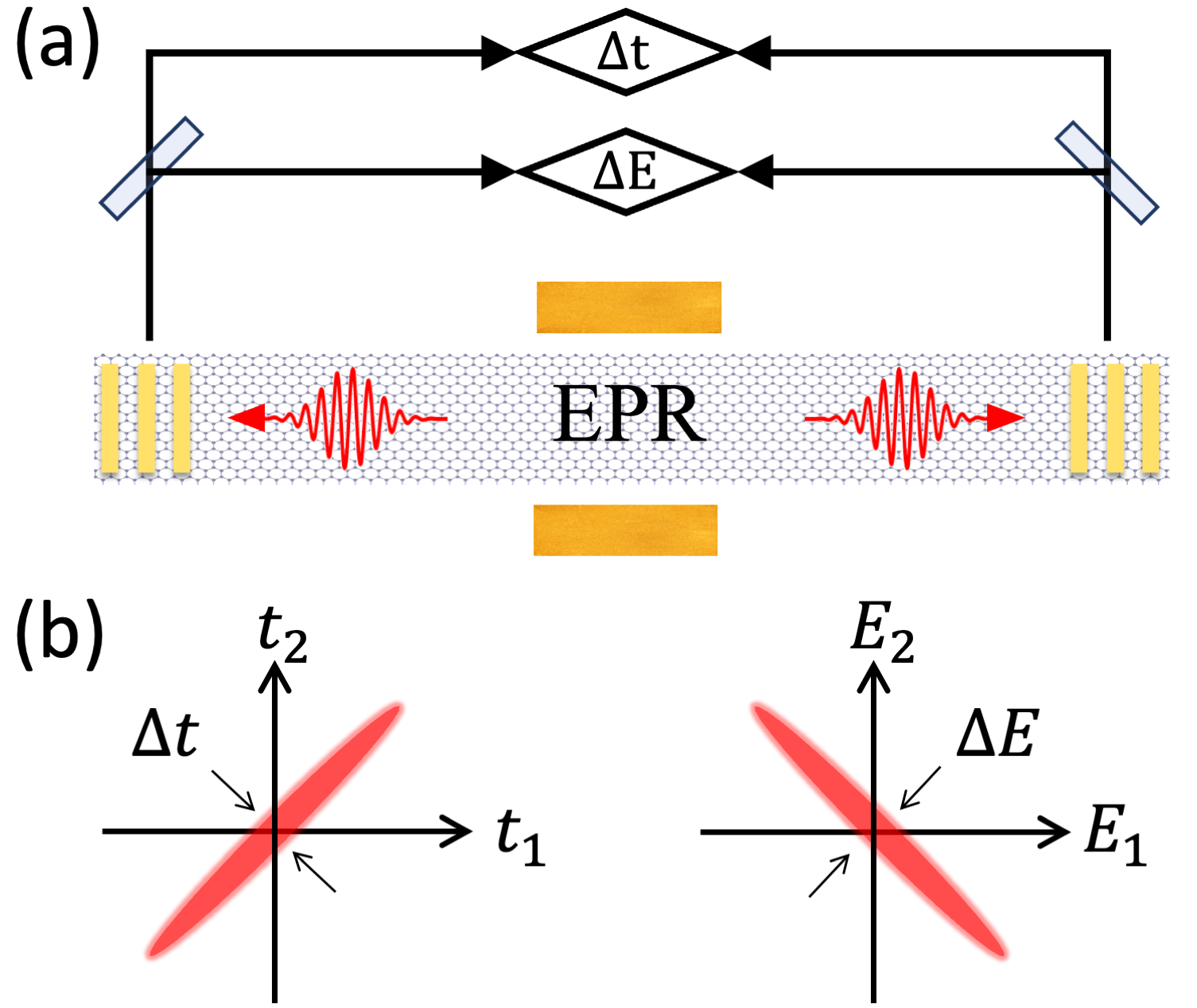
Figure 4: (a) Schematic of the experiment setup for coincidence measurement of the energy-time entanglement of the generated EPR plasmon pairs. The plasmon pair generator can be either a type-A (Fig. 1) or type-B device (Fig. 8). The vertical yellow bars are the grating structures to convert plasmons into far field photons. (b) Illustration of the time (left) and energy (right) correlations. The widths of the ellipses are the $\Delta t$ (left) and $\Delta E$ (right).

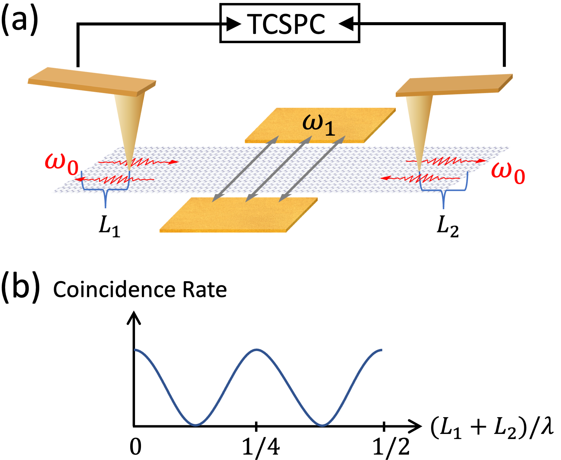
Figure 5: (a) The Franson scheme of measuring EPR entanglement with two scanning probes as the two interferometers. The plasmon pair generator can be either a type-A (Fig. 1) or type-B device (Fig. 8). (b) The coincidence rate as a function of $(L_{1}+L_{2})/\lambda$.

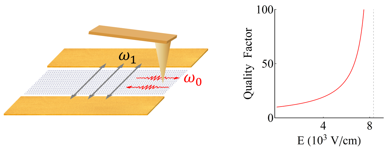
Figure 6: Near-field imaging of the parametric amplification of the mode-$0$ plasmons. The right figure is plotted for a type-A device using the parameters in Fig. 1. The parametric plasmon amplifier can also be a type-B device in Fig. 8.

To detect the position-momentum entanglement of a plasmon pair, one can place grating structures on both sides of the device which would convert the plasmons to far-field photons. Passing through the beam splitters, the photons are read either by single photon detectors [34, 59] which have good time precision or those with good energy resolution, as shown in Fig. 4. The coincidence rate measured by the former as a function of path length difference gives a time uncertainty $\Delta t$, while the spectrum correlation of the energy detectors gives the energy uncertainty $\Delta E$. The EPR entanglement is manifested in the relation $\Delta t\Delta E=\Delta x\Delta p<1/2$ [34, 60, 61]. This ‘energy time entanglement’ detection scheme is the same as that in Ref. [61] with the entangled photon source replaced by the plasmonic type-A device in Fig. 1 or type-B device in Fig. 8. Alternatively, homodyne detection experiments can measure the entanglement property of the squeezed state [34].

In addition, the Franson scheme [62, 40, 41] is also applicable as shown in Fig. 5. As mentioned in Sec. I, near field technique based on scanning probes has been successful in probing plasmons in graphene [2, 3, 4, 5, 6, 7, 8, 9, 10, 11, 12, 13]. To implement the Franson scheme, one needs two scanning probes, as shown in Fig. 5(a). The plasmons can either travel to the scanning probes directly or after being reflected by the edges of the ribbon, which we call short and long paths respectively. The coincidence detection arises from interference between the short-short and long-long paths. If the coincidence rate between the signals from two near field tips is measured as a function of $L_{1}\approx L_{2}$, the distance between each tip and the edge, it will oscillate as $R_{c}\sim\cos^{2}((L_{1}+L_{2})/\lambda)$, like that in Fig. 5(b). However, the condition $L\ll L_{i}\ll l$ needs to be satisfied. The first inequality guarantees that there are no single photon (or ‘short-long’ path) interference contributions, and the second inequality ensures that plasmon damping is not important. Note that in a prior work on measuring plasmon entanglement [63], the interfering particles were actually photons in optical fibers. In the proposed scheme (Fig. 5) the interference occurs between plasmons. Additionally, our implementation involves highly confined terahertz-infrared plasmons and scanning probes operating on deeply subdiffractional length scales.

One can also probe the classical effects. If the pump field is comparable to the parametric instability threshold, the enhancement of plasmon lifetime can be detected. Upon pumping of the $\omega_{1}$ mode of the type-A device in Fig. 1 (or type-B in Fig. 8), the $\omega_{0}$ modes with momenta $q$ and $-q$ are parametrically driven such that their effective damping rate is reduced to $\gamma-\kappa$ (see Appendix B), and their quality factor is boosted to $\omega_{0}/(\gamma-\kappa)$, as shown in Fig. 6. In a scanning near-field experiment, its manifestation is simply increased propagation length of the plasmons. One can also measure near field DFG using classical interference between the signal and idler in these experiments, which is discussed in Appendix F.

III Plasmon generation by the third-order nonlinearity

In this section we study the effects of third order nonlinearity [15, 64, 65, 19, 21, 24] on plasmon interactions which occurs already in the long wavelength limit. This nonlinearity originates from the linearity of the dispersion of Dirac quasiparticles in graphene which breaks Galilean invariance [24]. At low frequency $\omega\ll\varepsilon_{F}$, inter-band effects can be neglected and the third order nonlinear conductivity $\sigma^{(3)}$ in graphene assumes the third order ‘Drude’ form

$$\sigma^{(3)}_{ilmn} =\frac{iD^{(3)}}{\omega_{1}\omega_{2}\omega_{3}}\Delta_{ilmn}\,$$ (21)

both in the kinetic [66] and hydrodynamic [24] regimes where $\omega_{i}$ are the frequencies of the three electric fields that generate the third order current together. The symmetric tensor $\Delta_{ilmn}$ is the sum of all isotropic tensors $\Delta_{ilmn}=\delta_{il}\delta_{mn}+\delta_{im}\delta_{ln}+\delta_{in}\delta_{lm}$. Close to zero temperature ($T\ll\mu$), the third order optical weight is predicted to be $D^{(3)}=\frac{1}{24\pi}\frac{e^{4}v_{F}}{\hbar^{3}k_{F}}$ in the kinetic regime and twice as large in the hydrodynamic regime [24]. In what follows, we assume the system is the kinetic regime since we are mostly interested in the mid infrared plasmons whose frequencies are larger than the typical electron-electron scattering rate [23, 24].

III.1 FWM Hamiltonian

We start with the plasmonic effective Lagrangian of an electronic system whose linear conductivity is in the dissipation-less Drude form: $\sigma_{jk}=\frac{iD/\pi}{\omega}\delta_{jk}$ where $D$ is the Drude weight. In the near field approximation (meaning there is only longitudinal electric field and no magnetic field) and in the gauge $A^{\mu}=(0,\mathbf{A})$ for the electric field where $\mathbf{A}$ is the vector potential viewed as the plasmonic field, the Lagrangian is

$$L =\int d^{3}r\left(\frac{1}{8\pi c^{2}}\dot{\mathbf{A}}^{2}-\frac{D}{2\pi c^{2}}\mathbf{A}^{2}\delta(z)\right)+L^{(3)}$$

$$=\sum_{q}\left(\frac{1}{8\pi c^{2}}\frac{2}{|q|}\dot{A}_{-q}\dot{A}_{q}-\frac{D}{2\pi c^{2}}A_{-q}A_{q}\right)+L^{(3)}\,$$ (22)

where $c$ is the speed of light. The first term is the electric field energy and the second term has the interpretation of the center of mass kinetic energy of the charge carriers. For two dimensional (2D) Drude conductors modeled as the $x$-$y$ plane embedded in 3D space, since the current is localized on the 2D plane, the second term of the top line in Eq. (22) is nonzero only on the plane. In the second line of Eq. (22), $\mathbf{A}_{q}=\hat{q}A_{q}$ are the Fourier components of $\mathbf{A}$ evaluated on the 2D plane. The $2/|q|$ comes from integrating over the fields exponentially decaying into the three dimensional (3D) space. Note that the summation is over $\mathbf{q}=(q_{x},q_{y})$, and instead of three, there is only one plasmon mode for each $\mathbf{q}$ since the field is constrained to be longitudinal. The resulting Euler-Lagrange equation of motion for $A_{q}$ yields the 2D plasmon dispersion $\omega_{q}=\sqrt{2Dq}$ where the Drude weight is $D=v_{F}k_{F}e^{2}/\hbar$ for graphene at zero temperature. Quantization of the plasmonic field

$$A_{q}=i\hat{q}A_{qu}(a_{q}+a_{-q}^{\dagger}),\quad A_{qu}/c=\sqrt{\pi\hbar\omega_{q}/(2SD)}$$ (23)

leads to the Hamiltonian

$$H=H_{0}+H^{(3)},\quad H_{0}=\sum_{q}\hbar\omega_{q}\left(a_{q}^{\dagger}a_{q}+\frac{1}{2}\right)$$ (24)

where $S$ is the area of the sample.

The $H^{(3)}=-L^{(3)}$ contains products of four plasmonic creation and annihilation operators. It describes FWM which is caused by the third order optical conductivity $\sigma^{(3)}$. Writing the third order current $j^{(3)}$ in terms of vector potentials, Eq. (21) indicates $j^{(3)}_{i}=\Pi_{ilmn}A^{l}A^{m}A^{n}/c^{3}\,$ and the interaction Hamiltonian

$$H^{(3)}= -\frac{1}{4c^{4}}\int d^{2}r\Pi_{ilmn}A^{i}A^{l}A^{m}A^{n}$$

$$= -\frac{D^{(3)}}{4c^{4}}\sum\Delta_{ilmn}A^{i}_{q_{1}}A^{l}_{q_{2}}A^{m}_{q_{3}}A^{n}_{q_{4}}\,$$ (25)

where the kernel $\Pi_{ilmn}=D^{(3)}\Delta_{ilmn}$ is perfectly local in space and time, and the summation runs over all $q_{i}$ constrained by $q_{1}+q_{2}+q_{3}+q_{4}=0$ due to momentum conservation. Note that although Eq. (25) is a negative $\phi^{4}$ term in this bosonic field theory, the system is stable due to higher order nonlinear couplings.

III.2 Spontaneous four wave mixing

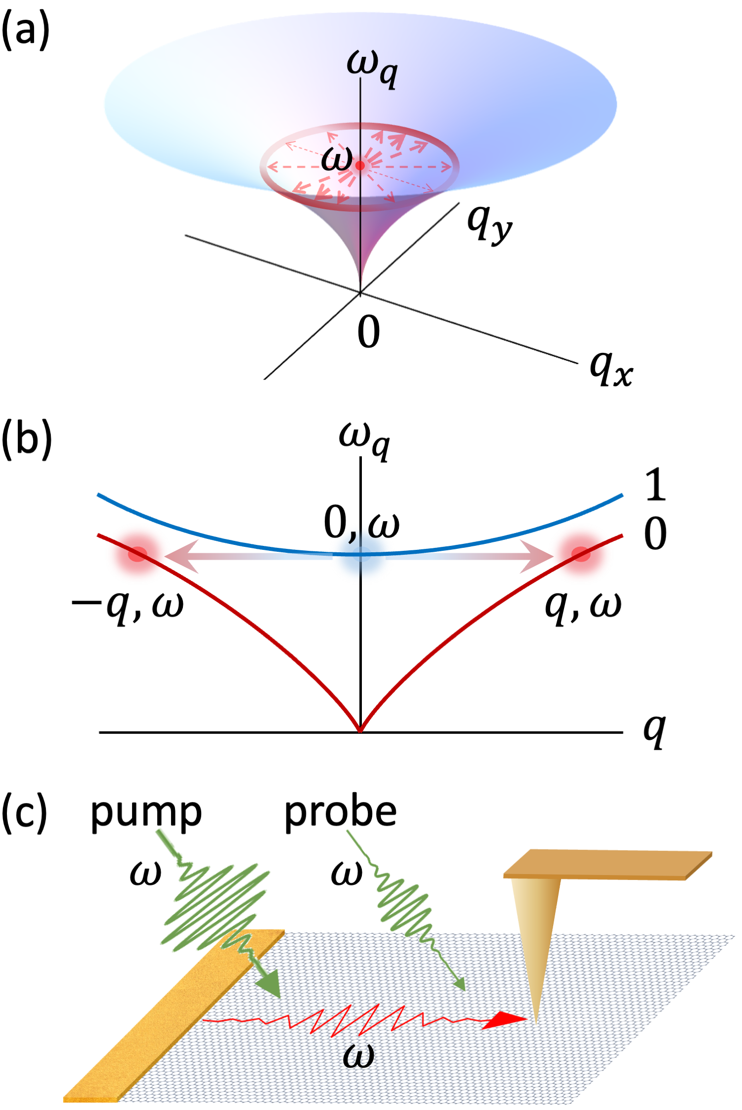
Figure 7: (a) Generation of entangled plasmon pairs due to spontaneous four wave mixing. The red dot at the center represents the pump. The red circle on the plasmon disperion curve represents the generated plasmons at the same frequency as the pump but nonzero momenta. The opacity of the circle and thickness of the arrows show the angular dependence of the pair generation intensity. (b) The decay of two mode-1 plasmons into a pair of entangled mode-0 plasmons on a graphene ribbon (same as type-A device in Fig. 1 but without doping gradient) due to spontaneous FWM. (c) The schematic of a near field measurement of the enhanced plasmon lifetime on a type-C device.

This subsection discusses spontaneous FWM shown in Fig. 7 in uniformly doped graphene. Eq. (25) implies that entangled plasmon pairs with frequency $\omega$ can be generated by incident light of the same frequency. We model far field photon incident on the graphene plane by an uniform AC electric field with amplitude $E_{0}=\omega A_{0}$ in $\hat{y}$ direction, and represent it by the vector potential $\mathbf{A}_{0}=\hat{y}A_{0}(e^{-i\omega t}+e^{i\omega t})\,$ where we have assumed $A_{0}$ to be real without loss of generality. When two fields in the product are replaced by the source $\mathbf{A}_{0}$, Eq. (25) becomes

$$H^{(3)} =-\sum_{q_{x}>0}g^{(3)}_{q}(t)(a_{q}+a_{-q}^{\dagger})(a_{-q}+a_{q}^{\dagger})\,$$ (26)

where the pair generation strength is

$$g^{(3)}_{q}(t) =\frac{1}{8}\hbar\omega_{q}\xi_{\omega}^{2}\left(1+2\sin^{2}\theta_{q}\right)\left(2+e^{-2i\omega t}+e^{2i\omega t}\right)\,$$ (27)

and $\theta_{q}$ is the angle of the plasmon momentum $q$ relative to the $\hat{x}$ axis. We have defined the dimensionless small parameter

$$\xi_{\omega}=\frac{eE_{0}/\omega}{\hbar k_{F}}\,$$ (28)

which controls the strength of FWM and other third order effects in graphene. In Eqs. (24) and (26), it is enough to consider terms close to resonance in the interaction picture. The number conserving terms in Eq. (26) like $a_{q}a_{q}^{\dagger}$ imply the field induced Kerr shift [33] of the plasmon frequency, which are red shifts in graphene due to its negative third order conductivity [24]. The terms like $e^{-2i\omega t}a_{q}^{\dagger}a_{-q}^{\dagger}$ lead to pair generation in the weak interaction regime ($g^{(3)}Q/\omega\ll 1$ where $Q=\omega/\gamma$ is the plasmon quality factor) and two mode squeezing (instability) in the strong interaction regime ($g^{(3)}Q/\omega>1$).

In the weak interaction regime, the plasmons with exactly the same frequency as $\omega$ are generated as entangled pairs and with an angular distribution of $\left(1+2\sin^{2}\theta_{q}\right)^{2}$, as shown in Fig. 7(a). The pair generation rate is determined by Fermi’s golden rule (analogous to Eq. (9)):

$$\Gamma=\frac{2\pi}{\hbar}\langle|g^{(3)}|^{2}\rangle_{\theta}\cdot\frac{S}{16\pi}\frac{\omega^{3}}{D^{2}}\,$$ (29)

where $\langle\rangle_{\theta}$ means angular average, the second part comes from the 2D plasmon density of states and we have assumed $\omega\gg T$ so the relevant plasmons are not occupied in equilibrium. The resulting dimensionless generation rate is

$$\frac{\Gamma}{\omega}=\frac{9}{2^{10}}\xi^{4}S\frac{\omega^{4}}{\alpha_{g}^{2}v_{F}^{2}\omega_{F}^{2}}\,.$$ (30)

For $n=10^{12}\,\mathrm{cm}^{-2}$, $E_{0}=10^{3}\,\mathrm{V/cm}$ and $S=1\,\mathrm{\mu m}^{2}$, we have $\Gamma/\omega=3.2\times 10^{-8}$. This leads to superior generation rates compared with conventional FWM sources, as we will discuss in Sec. IV. Since there is no need to break the inversion symmetry, this effect could be observed simply using uniformly doped graphene, which we call the type-C device. One may also use the ribbon in Fig. 1(a) but a lateral $p$-$n$ junction is no longer necessary. The spontaneous FWM process in a transversely pumped ribbon is illustrated in Fig. 7(b). To distinguish the generated entangled plasmon pairs from the linearly excited plasmons, the key experimental signature would be satisfaction of the EPR criterion [34] in the quadrature measurement in Fig. 4 or the nonlocal interference phenomenon in the Franson experiment in Fig. 5.

In the strong interaction regime, the plasmons are squeezed in pairs and experience parametric amplification. The resulting relative exponential growth rate is (similar to Eq. (17))

$$Q_{g}^{-1}=\frac{|g^{(3)}_{q}|}{\hbar\omega}=\frac{1}{8}\xi^{2}\left(1+2\sin^{2}\theta_{q}\right)\,$$ (31)

for the the plasmons propagating in $\theta_{q}$ direction, which agrees with the classical result (see Appendix E). In a typical near field experiment shown in Fig. 7(b), this reduces the plasmon damping rate from $\gamma$ to $\gamma-g_{q}^{(3)}/\hbar$. Therefore, to overcome the typical damping rate $\gamma\sim 0.1\omega$ of graphene plasmons, one needs $\xi\sim 0.3$ which requires a pump field of $E_{0}\sim 10^{5}\,\mathrm{V/cm}$ for $n=10^{12}\,\mathrm{cm}^{-2}$ and $\omega=30\,\mathrm{THz}$.

III.3 Spontanenous PDC in current carrying graphene

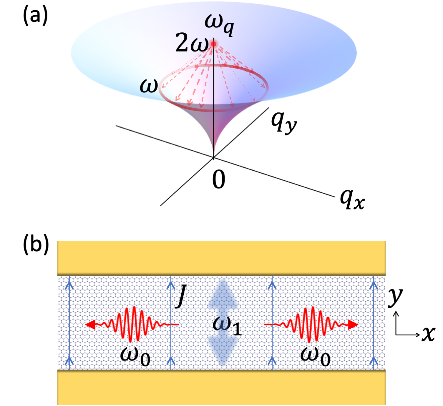
Figure 8: (a) Parametric down conversion of the pump of frequency $2\omega$ into pairs of subharmonic plasmons of frequency $\omega$ in current carrying graphene. (b) Realization in a ribbon (type-B device) which is similar to the type-A device in Fig. 1 except that the density gradient is replaced by a dc current $J$ flowing between the contacts.

The third order nonlinearity can also lead to PDC in a current-carrying graphene, as shown in Fig. 8. This effect can also be understood as FWM with one “pump wave” in Eq. (25) replaced by a dc current flow ($\omega=0$). If the other pump source has frequency $2\omega$, then the process looks like a PDC: $2\omega\rightarrow\omega+\omega$. Another point of view is that the dc current with flow velocity $u$ breaks the inversion symmetry, resulting in a nonzero second order nonlinear conductivity $\sigma^{(2)}\sim\frac{u}{v_{F}}\frac{e^{3}v_{F}}{\hbar^{2}}\frac{1}{\omega^{2}}$. To leading order in the dc current $J=enu$, the equations from subsection III.2 can be directly applied to the present case. We assume that the pump field is polarized parallel to the dc current, such that the PDC Hamiltonian is the same as Eqs. (26) and (27) but with $\xi_{\omega}^{2}$ replaced by $\xi_{2\omega}\xi_{0}$ where $\xi_{0}=eE_{\text{dc}}/(\gamma_{\text{dc}}\hbar k_{F})\approx u/v_{F}$ is the dimensionless parameter due to the dc electric field $E_{\text{dc}}$ that drives the dc current.

In the weak pump regime, entangled subharmonic plasmon pairs at frequency $\omega$ are generated with the angular distribution of $\left(1+2\sin^{2}\theta_{q}\right)^{2}$ in an infinite graphene sheet, same as that of spontaneous FWM. Summed over all angles, the total relative generation rate is the same as Eq. (30) but with with $\xi^{4}$ replaced by $\xi_{2\omega}^{2}\xi_{0}^{2}$. To measure the entanglement property of the emitted pairs, one can use the graphene ribbon in Fig. 8(b) as a plasmon pair source to perform either the energy-time entanglement measurement in Fig. 4 or the Franson scheme in Fig. 5. In the ribbon, the generated subharmonic pairs are not in every direction, but can only propagate along $\hat{x}$ (similar to Fig. 1(b)) with the generation rate described by roughly the same formula as that for an infinite sheet. For $n=10^{12}\,\mathrm{cm}^{-2}$, $\omega_{1}=2\omega=30\,\mathrm{THz}$, $E_{0}=10^{3}\,\mathrm{V/cm}$, a ribbon size of $S=0.2\,\mathrm{\mu m}\times 5\,\mathrm{\mu m}$ and a dc current of $J=0.16\,\mathrm{mA/\mu m}$ corresponding to $u=0.1v_{F}$, one has $\xi_{0}\approx 0.1$ and a normalized generation rate of $\Gamma/\omega\approx 0.9\times 10^{-6}$ from this type-B source.

In the strong pump regime, the plasmon lifetime is enhanced. The pump induced relative growth rate of plasmons of frequency $\omega$ is

$$Q_{g}^{-1}=\frac{1}{16}\xi_{2\omega}\xi_{0}\Delta_{ilmn}\hat{q}_{i}\hat{q}_{l}\hat{E}_{m}\hat{J}_{n}\,,$$ (32)

similar to Eq. (31). Here $\hat{X}$ means the unit vector along $X$ and $\hat{\mathbf{q}}$ is the unit vector of the momentum of the subharmonic plasmon. For a current of $J=0.5\,\mathrm{mA/\mu m}$ at the doping level of $n=10^{12}\,\mathrm{cm^{-2}}$ and under a pump field of $3\times 10^{5}\,\mathrm{V/m}$ at $\omega_{1}=2\omega=30\,\mathrm{THz}$ polarized along $\hat{y}$, the subharmonic plasmon running along $\hat{y}$ has a relative growth rate of $Q_{g}^{-1}\approx 0.03$, while those along $\hat{x}$ has a growth rate of $Q_{g}^{-1}\approx 0.01$, comparable to the plasmon loss at low temperatures [9].

III.4 Field enhancement in a ribbon

From previous discussion, high field is essential to make the proposed devices practical. By design, these devices naturally enhance the incident field by two mechanisms, helping to achieve this goal. First, as discussed in Sec. II.3(a), the split gate for type-A device in Fig. 1, or the contacts for type-B device in Fig. 8(b), act as antennas. They enhance the pump field by a factor of $F=E/E_{v}=\lambda_{v}/(2\pi w_{s})\approx 10$ [49] for the channel width $w_{s}=200\,\mathrm{nm}$ and the vacuum wave length of the pump light $\lambda_{v}\approx 10\,\mathrm{\mu m}$ at $\omega_{1}=30\,\mathrm{THz}$. Second, close to the resonance at $\omega_{1}$ with the gapped mode of the ribbon (see, e.g., Fig. 1(b) and Fig. 7(b)), there is another field enhancement factor of $F_{Q}=\xi_{f}\frac{\omega_{1}^{2}}{(\omega-\omega_{1}+i\gamma)(\omega+\omega_{1}+i\gamma)}$ where $\xi_{f}$ is an $O(1)$ shape factor, see Eqs. (11) and (63). On resonance, this leads to a field enhancement factor of $F_{Q}\sim Q\sim 10$.

The antenna effect together with the resonance field enhancement gives a net enhancement factor of $QF\sim 100$. Therefore, the spontaneous PDC rate in the type-B device (Fig. 8) is enhanced by a factor of $(QF)^{2}$ while the spontaneous FWM rate in a ribbon is enhanced by $(QF)^{4}$. Similarly, to reach a pump field of $10^{5}\,\mathrm{V/m}$ for parametric instability, the external incident field just needs to be of the order of $10^{3}\,\mathrm{V/m}$.

Note that the resonant field enhancement also occurs in photonic cavities such as micro-ring resonators [67, 68, 69, 70, 40]. In our devices, the vacuum photons play the role of the waveguide photons in the bus waveguide therein, and the graphene ribbon plays the role of the ring resonator. Unlike the plasmon modes in the nano-ribbon whose line width is dominated by intrinsic damping, the field enhancement on resonance in the micro-rings scales as $\sqrt{Q}$ instead of $Q$ [68] because the line width $\gamma_{p}$ of the photon modes in the micro-ring resonator is dominated by radiation leakage into the bus waveguide. As a result, the enhancement of the FWM pair generation rate due to resonant pumping scales as $Q^{2}$, see, e.g., Eq. 4 of Ref. [67]. Note also that in both our devices (short devices with length $L_{0}\ll l$) and photonic cavities, the resonance conditions with the generated modes contributes another factor of $Q$ to the enhancement of the generation rate.

IV Discussion and experimental outlook

PDC Devices	Frequency	$Q$	$\chi^{(2)}$ ($\,\mathrm{cm/V}$)	Generation Rate ($\,\mathrm{s^{-1}mW^{-1}}$)
Graphene type-A device (Fig. 1(a))	$4\,\mathrm{THz}$	$10-100$	$2\times 10^{-6}$	$9\times 10^{11}$
Graphene type-B device (Fig. 8(b))	$15\,\mathrm{THz}$	$10-100$	$3\times 10^{-6}$	$2\times 10^{12}$
Semiconductor coupled quantum wells [71, 47, 72]	$1-50\,\mathrm{THz}$	—	$\sim 10^{-6}$	—
LiNbO3 [73]	$0.79\,\mathrm{eV}$	—	$2\times 10^{-10}$	$2\times 10^{7}$
AlN [74]	$0.80\,\mathrm{eV}$	$1\times 10^{5}$	$4\times 10^{-11}$	$6\times 10^{6}$
FWM Devices	Frequency	$Q$	$\chi^{(3)}$ ($\,\mathrm{cm^{2}/V^{2}}$)	Generation Rate ($\,\mathrm{s^{-1}mW^{-2}}$)
Graphene type-B device with no DC current	$30\,\mathrm{THz}$	$10-100$	$4\times 10^{-14}$	$6\times 10^{14}$
AlGaAs on Insulator  [40]	$0.80\,\mathrm{eV}$	$1\times 10^{6}$	$7\times 10^{-17}$	$2\times 10^{10}$
Silicon on Insulator [75, 76]	$0.80\,\mathrm{eV}$	$\sim 10^{5}$	$4\times 10^{-17}$	$2\times 10^{8}$
InP [77]	$0.83\,\mathrm{eV}$	$4\times 10^{4}$	$2\times 10^{-16}$	$1\times 10^{8}$
Si3N4 [78]	$0.80\,\mathrm{eV}$	$2\times 10^{6}$	$4\times 10^{-19}$	$4\times 10^{6}$

Table 1: Comparison of graphene with conventional platforms for entangled photon generation following that in Ref. [40]. Although plasmons in these graphene devices can work in a broad frequency range from terahertz to infrared, we picked specific frequencies for estimations in the table. For graphene type-A device, the plasmon frequency is shown in Fig. 1(b) while for type-B device (with a current flow velocity of $u=0.1v_{F}$) and FWM, we used a pump frequency of $30\,\mathrm{THz}$. We used $a=200\,\mathrm{nm}$ and the quality factor of $Q=10$ for all the graphene devices. Since we are using the Gaussian unit system while the majority of nonlinear optics literature uses the SI unit, we translated from the latter in the literature to the former in this table. The refraction indices used for conversion of $\chi^{(3)}$ are AlGaAs: $N=3.2$ at $\lambda=1.55\,\mathrm{\mu m}$, Silicon: $N=3.5$ at $\lambda=1.55\,\mathrm{\mu m}$, InP: $N=3.4$ at $\lambda=1.49\,\mathrm{\mu m}$, Si₃N₄: $N=2.0$ at $\lambda=1.55\,\mathrm{\mu m}$.

We proposed several graphene spontaneous PDC and FWM devices which have promising quantum information applications [79] as efficient sources of entangled plasmon pairs, photon-plasmon converters and plasmon amplifiers [80, 81, 82, 83, 84], etc., for future quantum plasmonic/polaritonic circuits. These plasmons are in the THz-Infrared spectra range, which is an important energy range in condensed matter physics where superconductivity, magnetism, spin liquid, fractional quantum hall effect and other correlated phenomena are relevant. The quantum sources proposed here may enable quantum imaging [85] and sensing [86] of these novel states of matter.

Let us compare our devices with conventional photonic PDC sources. In photonic PDC, the nonlinearity is usually characterized by a nonlinear susceptibility $\chi^{(2)}$, which has the unit of inverse electric field. We can convert the 2D conductivity $\sigma^{(2)}$ to an effective 3D nonlinear susceptibility $\chi^{(2)}$ as follows. The 2D nonlinear susceptibility (in the Gaussian unit system) is [87] $\chi^{(2)}_{\mathrm{2D}}=i\sigma^{(2)}/\omega_{0}$. For the type-A device which is a ribbon with half width $a$, the extent of the electric field of the plasmon in the out-of-plane direction is $1/q_{0}\sim a$. Hence, the effective 3D nonlinear susceptibility is $\chi^{(2)}\sim\chi^{(2)}_{\mathrm{2D}}/a\sim 1/(ek_{F}^{2})$. For $k_{F}=\sqrt{\pi}\times 10^{6}\,\mathrm{cm^{-1}}$ corresponding to carrier density $n=10^{12}\,\mathrm{cm}^{-2}$, we find $\chi^{(2)}\sim 2\times 10^{-6}\,\mathrm{cm/V}$, which is much larger than that of conventional photonic media, e.g., LiNbO₃ [73, 41], but is of the same order as $\chi^{(2)}$ in sophisticated photonic waveguides made of coupled quantum wells  [71, 47, 72], see Table 1. Nevertheless, a more important figure of merit is the dimensionless decay factor

$$\frac{\Gamma}{\omega_{0}}\sim|\chi^{(2)}|^{2}\frac{\hbar\omega_{0}}{a^{3}}$$ (33)

(same as Eq. (10) noting that $g^{(2)}\sim\chi^{(2)}\omega_{0}^{3/2}a^{-1}L^{-1/2}$ ) of a waveguide mode into subharmonic modes due to spontanenous PDC. Due to strong mode confinement ($a\ll c/\omega_{0}$), this figure of merit is much larger than those of photonic devices. Physically, this is because electric field of a single plasmon in our device is much larger than that of a single photon.

As discussed in Sec. III.3, a comparable $\chi^{(2)}$ can also be achieved in a type-B device where inversion symmetry is broken by applying a DC current flow to an uniformly doped ribbon if the flow velocity is moderately fast: $u>0.1v_{F}$.

We also consider the FWM [33] in Sec. III.2, a third-order nonlinear effect. Such a process does not require inversion-symmetry breaking and can take place in either a ribbon or a plain graphene sheet (type-C device in Fig. 7). This plasmon instability requires a relatively strong incident field controlled by the small parameter $\chi^{(3)}$, but it may be easier to realize experimentally since there is no specific requirement for the nano structure. Compared with other nonlinear materials, $\chi^{(3)}=i\sigma^{(3)}/(\omega a)$ in graphene is much stronger, as shown in Table 1.

A brief discussion of units conversion is in order. The Gaussian unit system defines the 3D nonlinear susceptibilities in terms of the effective dielectric function $\epsilon=1+4\pi\left[\chi+\chi^{(2)}E+\chi^{(3)}E^{2}+...\right]$ while the SI system defines them as $\epsilon/\epsilon_{0}=1+\chi_{\text{SI}}+\chi^{(2)}_{\text{SI}}E+\chi^{(3)}_{\text{SI}}E^{2}+...$ [33] where $\epsilon_{0}$ is the vacuum permittivity. Therefore, besides converting the units of electric fields, there is an additional $4\pi$ factor: $\chi^{(n)}=\chi^{(n)}_{\text{SI}}/(4\pi)$. The unit $\,\mathrm{m^{2}/W}$ is also used in the literature [75, 40] for third order nonlinearity $N_{3}$ defined as $\delta N=\frac{1}{2N}\chi^{(3)}_{\text{SI}}E^{2}=\frac{4\pi}{2N}\chi^{(3)}E^{2}\equiv N_{3}P$ where $N=\sqrt{1+4\pi\chi}$ is the linear refraction index, $\delta N$ is the change of effective refraction index due to third order nonlinearity and the pump field, and $P$ is the power flux of the pump field. Therefore, besides converting $\,\mathrm{m^{2}/W}\rightarrow 0.00132806\,\mathrm{m^{2}/V^{2}}$, one also needs the conversion $\chi^{(3)}=\frac{N}{2\pi}N_{3}$ to obtain the $\chi^{(3)}$ in Gaussian unit.

We note that the properties of the type-A device may have substantial temperature dependence arising from the middle of the ribbon [Fig. 1(a)] where the system is close to charge neutrality. The gapped mode is an anti-symmetric charge oscillation between the upper and lower half of the strip, and thus strongly depends on the conductivity at the middle of the junction where the carriers are thermally excited electrons and holes. Therefore, the frequency of the gapped mode (the shape factor $\xi_{1}$ in Sec. II) increases with temperature. In our derivation, we included only the intraband contributions [54, 20, 51, 23] to the second order nonlinear conductivity [Eq. (82)]. Close to the middle of the junction where $\mu\lesssim\hbar\omega$, interband contributions may be important. There the total $\sigma^{(2)}$ is suppressed by a factor of $(\mu/\hbar\omega)^{M}$ with $M\geq 2$ compared to the intraband expressions used in this paper, but $\sigma^{(2)}$ may diverge at the narrow region where $\mu=\hbar\omega$ at the interband threshold for Pauli blocking [87, 20, 54, 51, 88, 89]. This divergence is rounded by nonzero temperature, and would thus lead to substantial temperature dependence if included. We note that even in homogeneously doped graphene, there are $3\sim 4$ orders of magnitude inconsistencies [90] between theories (e.g., Refs. [87, 20, 54, 51, 88]) and experiments [26, 25]. At this stage, it is premature to include such details in the model, and instead, we provide order of magnitude scaling results for the PDC. Incidentally, experiment and theory seem to agree for $\sigma^{(3)}$ [65].

As mentioned in Sec. I, generation of plasmons by PDC in graphene has also been considered by Ref. [51]. In that study, the pump and idler are far field photons. In contrast, here all three modes are plasmons such that frequencies are much lower and momenta are much larger, making this process much more efficient. Moreover, our proposed device involves an antenna that further increases the coupling efficiency to far field pump. As a result, the threshold power to achieve parametric instability is about four orders of magnitude lower than Ref. [51].

Since plasmons do not have the polarization degree of freedom (they are always longitudinally polarized), entanglement of polarization frequently discussed in quantum optics does not apply here. In plasmonics one focuses on the position-momentum (or energy-time) entanglement. For example, it has been shown this entanglement survives photon-plasmon conversion processes [31, 91, 63]. Here we proposed a scheme to directly generate and measure the entanglement of plasmon pairs on a chip using the modern tools of near field optics.

The following estimate shows that graphene will not be damaged by the strong electric field required. The incident light heats up the electron gas in graphene with the heating power $P_{\text{heat}}=2\mathrm{Re}[\sigma]|E|^{2}$ and electron phonon scattering provides its cooling channel. The cooling power is approximated by $P_{\text{cool}}=C_{v}\gamma_{c}(T_{e}-T_{l})$ where $T_{e}$($T_{l}$) is the electron(lattice) temperature, $C_{v}\sim g(\varepsilon_{F})T$ is the heat capacity of the electron gas and $\gamma_{c}\sim 1\,\mathrm{ps}^{-1}$ is the cooling rate revealed by previous experiment [7]. The lattice is a good heat conductor and is assumed to stay at the same temperature as the environment. The balancing of heating and cooling $P_{\text{heat}}=P_{\text{cool}}$ determines the stationary electron temperature $T_{e}-T_{l}\sim\frac{1}{4\pi^{2}}\frac{\gamma}{\gamma_{c}}\frac{\varepsilon_{F}^{2}}{T}\xi^{2}$ where we have set the Boltzmann constant to one. At the typical doping level and frequency scale considered in this paper, for $T_{l}=300\,\mathrm{K}$ and $E=10^{4}\,\mathrm{V/cm}$, we conclude that $T_{e}-T_{l}\sim 6\,\mathrm{K}$ which is quite small compared to either room temperature or the Fermi energy.

We worked in the kinetic regime where plasmon frequency is much larger than the electron-electron scattering rate $\omega\gg\Gamma_{ee}$ [23]. In the low frequency hydrodynamic regime $\omega\ll\Gamma_{ee}$ [92, 81, 23, 93, 94, 95, 96, 97, 98], the nonlinear conductivities are similar in magnitude as long as the temperature is not much larger than chemical potential [23, 24, 99]. Therefore, our estimate of the generation rates should apply as well to the collective modes in the hydrodynamic regime such as the charged ‘demons’ [92, 81, 23, 93, 94, 96, 97]. However, in the case of $T\gg\mu$, the demons become almost charge neutral, driven mainly by kinematic pressure, and the physics could be quite different. It may be interesting to study nonlinear and quantum effects for these collective modes [100, 24].

Since the ribbon width is much larger than the lattice constant, the Dirac dispersion approximation for the electrons in graphene are valid. We used the ‘local’ approximation to compute the plasmonic modes, which neglects dependence of the optical conductivity $\sigma(\omega,q)$ on the field wave vector $q$, see Appendix C.1. The nonzero $q$ effects enter $\sigma(\omega,q)$ as a power expansion in the dimensionless small number $v_{F}^{2}q^{2}/\omega^{2}$ [23, 8, 11], see, e.g., the supporting information of Refs. [23, 11]. For the relevant modes of the ribbons such as mode-1 in Fig. 1, one has $q\approx 2\pi/(4a)$ and $v_{F}q/\omega\approx 0.36$, meaning that the devices are indeed in the local regime. As an estimate, the leading order nonlocal correction $\delta\omega_{1}$ to the plasmon frequency $\omega_{1}$ is just $\frac{\delta\omega_{1}}{\omega_{1}}=\frac{1}{2}\frac{3}{4}(\frac{v_{F}q}{\omega})^{2}\approx 0.05$ in the kinetic regime we are considering. Therefore, the Drude (or ‘local’) approximation is well justified.

Extension of these nonlinear effects to polaritonic modes [101, 102, 103] beyond those in graphene is a meaningful future direction. For example, monolayer hexagonal boron nitride [104, 105] should exhibit strong second order optical nonlinearity due to broken inversion symmetry of the crystal lattice, and would be a natural platform for generating entanglement between the long lived hyperbolic phonon polaritons [106, 107, 108, 109, 110, 111, 112, 113, 114, 115]. Similar nonlinear processes exist for optical phonons in SiC [116], Josephson plasmons in layered superconductors [84, 117, 118, 119] and the collective modes in excitonic insulators [120, 121, 122, 123, 124].

Appendix A Summary of notations for the ribbon case

The main results of this paper are written in terms of various “shape” parameters and physical quantities such as size ($a$, $L$), Fermi momentum ($\varepsilon_{F}$), Fermi velocity ($v_{F}$), electric field ($E$) and frequency ($\omega$). Most of the shape parameters are dimensionless numbers of the order of unity. They are $S_{0}^{\prime}$, $S_{1}^{\prime}$, $\alpha^{\prime}$, $\eta^{\prime}$, $\xi_{0}$, $\xi_{1}$, $\xi_{g}$, $\xi_{\text{df}}$, $\xi_{\beta}$, and $\xi_{Q}$. Their definitions for the case of a ribbon are as follows:

$$S_{0}^{\prime} =\int_{-1}^{1}dy\tilde{\sigma}(y)|\mathbf{\tilde{E}}_{0}|^{2}\,,$$

$$S_{1}^{\prime} =\int_{-1}^{1}dy\tilde{\sigma}(y)|\mathbf{\tilde{E}}_{1}|^{2}\,,$$

$$\alpha^{\prime} =\int_{-1}^{1}dy\tilde{\sigma}(y)\hat{\mathbf{e}}\cdot\mathbf{\tilde{\mathbf{E}}}_{1}\,,$$

$$\eta^{\prime} =q_{x}^{\prime 2}\int_{-1}^{1}dy\,\partial_{y}^{2}\varphi_{1}\,\varphi_{0}^{2}\,\tilde{g}(y)\,,$$

$$\xi_{v}(q) =\dfrac{\omega(q)}{\sqrt{\alpha_{g}(ak_{F})}v_{F}q}=\dfrac{\omega(q)}{v_{a}q}\,,$$

$$\xi_{0} =\xi_{v}(q_{0})\,,$$

$$\xi_{1} =\dfrac{\hbar\omega_{1}}{\sqrt{2e^{2}E_{F}/a}}\,,$$

$$\xi_{g} =\xi_{1}^{1/2}\frac{\eta^{\prime}}{S_{1}^{\prime 1/2}S_{0}^{\prime}}\,,$$

$$\xi_{\text{df}} =\frac{v_{a}}{v_{l}}\frac{\eta^{\prime}}{S_{1}^{\prime}S_{0}^{\prime 2}}\,,$$

$$\xi_{\beta} =\frac{1}{\xi_{1}^{3/2}}\,\frac{\alpha^{\prime}}{S_{1}^{\prime 1/2}}\,,$$

$$\xi_{Q} =\frac{\eta^{\prime}}{\xi_{1}^{2}}\,\frac{\alpha^{\prime}}{S_{0}^{\prime}S_{1}^{\prime}}\,.$$

The remaining ones, $S$, $\alpha$ and $|\tilde{\rho}|^{2}$, are just the corresponding dimensionless ones multiplied by $aL$, one half of the total area of the ribbon.

Appendix B Parametric oscillator

The spontanenous PDC process in Sec. II is similar to what happens in a parametric oscillator (PO) except that the former leads to two-mode squeezing while the latter corresponds to single-mode squeezing [57]. Optical POs are widely used to generate subharmonic light and to create entangled photon pairs. To make the paper self-contained, we review the basic theory of the PO in this Appendix.

A PO can be modeled with the equation of motion

$$\hat{L}x(t)=\left[\partial^{2}_{t}+\gamma\partial_{t}+\left(1+2\delta\cos\Omega t\right)\omega_{0}^{2}\right]x(t)=F(t)\,,$$ (34)

where $\Omega$ is the frequency of the pump modulating the natural frequency $\omega_{0}$ of the oscillator by a relative amount $\sim\delta$. The difference

$$\Delta=\Omega-2\omega_{0}$$ (35)

of $\Omega$ from the primary parametric resonance frequency $2\omega_{0}$ is referred to as the detuning. Given the initial conditions $x(0)$, $\dot{x}(0)\equiv\partial_{t}x(t)|_{t=0}$, the solution of Eq. (34) can be written in terms of the retarded Green’s function $G=G(t,t^{\prime})$:

$$\begin{split}x(t)&=\left.\left\{\left[\dot{x}(0)+\gamma x(0)\right]G-x(0)\partial_{t^{\prime}}G\right\}\right|_{t^{\prime}=0}\\ &+\int G(t,t-\tau)\Theta(t-\tau)F(t-\tau)d\tau\,,\end{split}$$ (36)

where $\Theta(t)$ is the Heaviside step-function. One simple example is $x(0)=0$, $\dot{x}(0)=1$, $F(t)\equiv 0$, in which case $x(t)=G(t,0)$.

As usual, the Green’s function is constructed from an arbitrary pair of linearly independent solutions $x_{1}(t)$, $x_{2}(t)$ of the homogeneous equation $\hat{L}x(t)=0$:

$$G(t,t^{\prime}) =\Theta(t-t^{\prime})\frac{x_{1}(t^{\prime})x_{2}(t)-x_{2}(t^{\prime})x_{1}(t)}{W(t^{\prime})}\,,$$ (37)

$$W(t) =x_{1}(t)\partial_{t}x_{2}(t)-x_{2}(t)\partial_{t}x_{1}(t)\,.$$ (38)

By virtue of the Abel formula, the Wronskian determinant [Eq. (38)] has the following $t$-dependence:

$$W(t)=W(0)e^{-\gamma t}\,.$$ (39)

One possible choice of $x_{1}(t)$ and $x_{2}(t)$ is

$$x_{1}(t) =e^{-\frac{1}{2}\gamma t}\mathrm{C}\left(\frac{4\omega_{0}^{2}-\gamma^{2}}{\Omega^{2}},\,-\frac{4\delta\omega_{0}^{2}}{\Omega^{2}},\,\frac{1}{2}\Omega t\right)\,,$$ (40)

$$x_{2}(t) =e^{-\frac{1}{2}\gamma t}\mathrm{S}\left(\frac{4\omega_{0}^{2}-\gamma^{2}}{\Omega^{2}},\,-\frac{4\delta\omega_{0}^{2}}{\Omega^{2}},\,\frac{1}{2}\Omega t\right)\,,$$ (41)

where $\mathrm{C}(a,b,z)$ and $\mathrm{S}(a,b,z)$ are the even and the odd Mathieu functions, respectively, as defined in Mathematica [125] (Mathematica notations are $\mathrm{MathieuC}[a,b,z]$ and $\mathrm{MathieuS}[a,b,z]$). These functions are normalized as $\mathrm{C}(a,0,z)=\cos(\sqrt{a}z)$, $\mathrm{S}(a,0,z)=\sin(\sqrt{a}z)$ for $b=0$.

From Eqs. (37)–(41), we conclude that

$$G(t,0)=\frac{x_{2}(t)}{\dot{x}_{2}(0)}\,,$$ (42)

so that an instability, i.e., the exponential growth of $G(t,0)$ is possible if $\mathrm{S}(a,b,z)$ is increasing faster than $e^{\frac{1}{2}\gamma t}$. This occurs if $|\delta|$ exceeds some threshold value $\delta_{c}=\delta_{c}(\gamma,\Delta)$. Conversely, the response function $G(t,0)$ exhibits exponential decay with time if $|\delta|<\delta_{c}$. Examples of such stable and unstable behaviors are shown in Fig. 9.

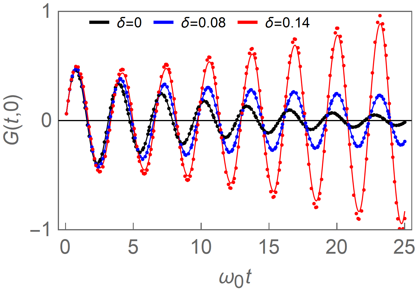
Figure 9: Behavior of the Green’s function $G(t,0)$ of Eq. (34) at several values of the modulation parameter $\delta$ at resonance $\Omega=2\omega_{0}$. The solid lines show the exact Green’s function [Eq. (37)], the dots are the approximations constructed from Eq. (51). The damping rate is $\gamma=0.1\omega_{0}$ corresponding to $\delta_{c}\approx 0.1$.

Approximate analytical calculation of $\delta_{c}$ can be done for low damping $\gamma\ll\omega_{0}$ and small detuning $\Delta\ll\omega_{0}$. Thus, one can show that

$$\delta_{c}\simeq\frac{\sqrt{\Delta^{2}+\gamma^{2}}}{\omega_{0}}\,,$$ (43)

in agreement with Fig. 9.

The derivation goes as follows. Let us seek a solution of Eq. (34) in the form

$$x(t)=A(t)e^{i\omega_{0}t}+B(t)e^{-i\omega_{0}t}\,$$ (44)

where $A(t)$, $B(t)$ are slowly varying. Matching the coefficients for the rapidly oscillating phase factors of Eq. (34), we obtain

$$\begin{pmatrix}2i\partial_{t}+i\gamma&&\omega_{0}\delta e^{i\Delta t}\\ \omega_{0}\delta e^{-i\Delta t}&&-2i\partial_{t}-i\gamma\end{pmatrix}\begin{pmatrix}A\\ B\end{pmatrix}=\begin{pmatrix}0\\ 0\end{pmatrix}.$$ (45)

To eliminate the factors $e^{\pm i\Delta t}$, we change variables to

$$A(t)=e^{\frac{i}{2}\Delta t}a(t)\,,\quad B(t)=e^{-\frac{i}{2}\Delta t}b(t)\,,$$ (46)

arriving at

$$\begin{pmatrix}2i\partial_{t}+i\gamma-\Delta&&\omega_{0}\delta\\ \omega_{0}\delta&&-2i\partial_{t}-i\gamma-\Delta\end{pmatrix}\begin{pmatrix}a\\ b\end{pmatrix}=\begin{pmatrix}0\\ 0\end{pmatrix}.$$ (47)

The general solution of this equation is

$$\begin{pmatrix}a\\ b\end{pmatrix}=e^{\lambda_{1}t}\begin{pmatrix}u_{1}\\ v_{1}\end{pmatrix}+e^{\lambda_{2}t}\begin{pmatrix}u_{2}\\ v_{2}\end{pmatrix}\,,$$ (48)

where

$$\lambda_{1,2}=-\frac{\gamma}{2}\pm\frac{i}{2}\sqrt{\Delta^{2}-(\omega_{0}\delta)^{2}}$$ (49)

are the growth rates and

$$\begin{pmatrix}u_{j}\\ v_{j}\end{pmatrix}=\begin{pmatrix}\omega_{0}\delta\\[5.0pt] \Delta-i\gamma-i\lambda_{j}\end{pmatrix},\quad j=1,2$$ (50)

are the corresponding eigenvectors. Two linearly independent solutions for $x(t)$ could be chosen as

$$x_{j}=e^{\lambda_{j}t}\left(u_{j}e^{i\frac{\Omega}{2}t}+v_{j}e^{-i\frac{\Omega}{2}t}\right),\quad j=1,2\,,$$ (51)

and the Green’s function can be constructed per Eq. (37). Assuming $\mathrm{Re}[\lambda_{2}]\geq\mathrm{Re}[\lambda_{1}]$, the instability threshold is determined by the condition

$$\mathrm{Re}[\lambda_{2}]=0\,,$$ (52)

which leads to Eq. (43). A comparison with the exact Green’s function confirms the validity of this approximation for small damping and detuning, such as $\gamma=0.1\omega_{0}$ and $\Delta=0$ in Fig. 9.

Consider now the response of the PO to a periodic driving source

$$F(t)=f_{\omega}e^{-i\omega t}+\text{c.c.}\,.$$ (53)

In the stable case, $|\delta|<\delta_{c}$, where the effect of the initial conditions disappears at long times, $x_{\omega}$ is the linear response to $F$:

$$x_{\omega}(t)=f_{\omega}e^{-i\omega t}\int\limits_{0}^{\infty}G(t,t-\tau)e^{i\omega\tau}d\tau+\text{c.c.}\,.$$ (54)

Without the pump, $G(t,t-\tau)$ is a function of $\tau$ only, and so the integral on the right-hand side reduces to a constant. Under pumping, $G(t,t-\tau)$ is periodic in $t$ with the period $2\pi/\Omega$. Accordingly, the Fourier spectrum of $x_{\omega}(t)$ becomes a frequency comb of Floquet harmonics $\omega+m\Omega$ where $m$ is an arbitrary integer. For small $\gamma$ and $\Delta$, however, it is easier to compute $x_{\omega}(t)$ not from Eq. (54) but from Eq. (47) supplemented with the appropriate right-hand side. The result is

$$x_{\omega}(t)= \frac{f_{\omega}e^{-i\omega t}}{(\omega-\nu_{1})(\omega-\nu_{2})}\left(\frac{\Omega-2\omega-i\gamma+\Delta}{4\omega_{0}}-\frac{\delta}{4}e^{i\Omega t}\right)$$

$$+\text{c.c.}\,.$$ (55)

Apparently, this approximation accounts only for the dominant Floquet harmonics: $\omega-\Omega$, $\omega$, and $\omega+\Omega$. In the complex plane of $\omega$, function $x_{\omega}$ (or the linear response kernel) has two poles, at $\nu_{1}$ and $\nu_{2}$, given by

$$\nu_{1,2}=\frac{\Omega}{2}+i\lambda_{1,2}=\omega_{0}+\frac{\Delta}{2}-\frac{i\gamma}{2}\mp\frac{1}{2}\sqrt{\Delta^{2}-(\omega_{0}\delta)^{2}}\,.$$ (56)

The pole $\nu_{2}$ has a larger imaginary part, which grows with $|\delta|$. At $|\delta|=\delta_{c}$, $\nu_{2}$ crosses over into the upper half-plane of $\omega$, signaling the instability.

Instead of a periodic driving source, we can consider a stochastic one, namely, a Langevin source defined by the two-point correlator

$$\big{\langle}F(t)F(0)\big{\rangle}=\frac{\gamma T}{\pi}\delta(t)\,.$$ (57)

In this case the total driving force $F(t)$ contains a continuum of Fourier harmonics, and the response $x(t)$ is obtained by integrating expressions like Eq. (55) over $\omega$. The stochastic drive leads to random fluctuations of $x$, causing a nonzero average power injection by the parametric pump into the system:

$$P=2\omega_{0}^{2}\delta\left\langle\cos\Omega t\,x\partial_{t}x\right\rangle\,.$$ (58)

A straightforward calculation based on Eqs. (55) and (58) yields

$$P=\frac{({\omega_{0}\delta})^{2}\gamma T}{\gamma^{2}+\Delta^{2}-(\omega_{0}\delta)^{2}}\,.$$ (59)

Finally, we generalize this result to the quantum case. We do not show a formal derivation, but sketch a more physical approach. The essential point is that the power injection $P$ by the pump is enabled by the nonzero quantum/thermal fluctuations of $x$. The starting point is a Hamiltonian of the total system (PO plus environment) in the form

$$H(t) =H_{\mathrm{PO}}-F(t)x+H_{\mathrm{env}}\,,$$ (60)

$$H_{\mathrm{PO}} =\frac{p^{2}}{2}+\frac{1}{2}\left(1+2\delta\cos\Omega t\right)\omega_{0}^{2}x^{2}\,.$$ (61)

The purpose of $H_{\mathrm{env}}$ is to describe the Langevin noise source and the dissipation effects. A standard device to achieve this is to use the Caldeira-Leggett model of a bath of harmonic oscillators. We surmise that the final answer for $P$ is similar to the classical Eq. (59) except the thermal energy $T$ is replaced by $\hbar\omega_{0}\left(n_{b}+\frac{1}{2}\right)$ where $n_{b}=1/(e^{\hbar\omega_{0}/T}-1)$ is the boson occupation number. Since the injected power increases the energy of the PO, the pump must be generating quanta of the PO motion. Dividing $P$ by the energy $2\hbar\omega_{0}$ of two such quanta, we obtain the pair generation rate

$$R=\frac{P}{2\hbar\omega_{0}}=\frac{\gamma}{\gamma^{2}+\Delta^{2}-(\omega_{0}\delta)^{2}}\,\frac{({\omega_{0}\delta})^{2}}{2}\left(n_{b}+\frac{1}{2}\right)\,.$$ (62)

Note that formally, in the quantum mechanical language, this nonperturbative result in the parametric pump $\delta$ can be obtained by computing the linear response to $\delta$ (bubble diagram) [120], with the boson propagators replace by the renormalized ones by $\delta$ [see Eq. (55)]. As shown by Eq. (62), at weak pumping, $R$ scales quadratically with $\delta$, consistent with Fermi’s Golden Rule. The precise match is obtained in the limit $\gamma\to 0$, $\omega_{0}\delta/\gamma\to 0$ where $R$ is nonzero only at the resonance, $R\propto\delta(\Delta)$. As $\delta$ increases, deviations from Fermi’s Golden Rule appear. As $\delta$ approaches the critical value $\delta_{c}$ [Eq. (43)], the pair generation rate diverges.

Lastly, expressing $\delta$ in terms of the coupling constant $g^{(2)}$ in Sec. II and integrating over the acoustic modes in the vicinity of $\omega_{0}$ we obtain Eq. (14).

Appendix C Derivation for the graphene ribbon (type-A device)

C.1 Plasmon modes on a generic nano structure

Unlike the uniform two-dimensional (2D) electron gas, a generic conducting nano structure [126, 127, 17] breaks the translational symmetry in at least one direction, and the plasmon modes can not be classified by 2D momenta. In this section, we define necessary profile functions describing the graphene nano island (e.g. a ribbon) such that the quantization could be described semi-analytically. Meanings of the dimensionless profile functions are summarized in Table 2.

The linear optical conductivity is assumed local and in the Drude form: $\mathbf{j}(\mathbf{r})=\hat{\sigma}(\mathbf{r})\mathbf{E}(\mathbf{r})=\frac{i}{\pi(\omega+i\gamma)}D(\mathbf{r})\mathbf{E}(\mathbf{r})$ where $D(\mathbf{r})$ is the local Drude weight. This holds for $\omega\gg v_{F}q$ where $q$ is the characteristic momentum corresponding to the plasmon modes and size of the nano structure. In the case of a graphene ribbon with $a$ being its half width, this momentum is roughly $q\approx\pi/(2a)$. We define the dimensionless conductivity profile function $\tilde{\sigma}$ by $\hat{\sigma}(\mathbf{r})=\hat{\sigma}\tilde{\sigma}(\mathbf{r})$ (or $D(\mathbf{r})=D\tilde{\sigma}(\mathbf{r})$) where $D$ is the maximum local Drude weight. Assume a certain plasmon mode has the charge density profile $\rho(\mathbf{r})=\rho\tilde{\rho}(\mathbf{r})$, its electric field profile is

$$\mathbf{E}(\mathbf{r})=-\nabla\hat{V}\rho(\mathbf{r})=\rho\tilde{\mathbf{E}}(\mathbf{r})\,,\quad\tilde{\mathbf{E}}(\mathbf{r})\equiv-\nabla\hat{V}\tilde{\rho}(\mathbf{r})$$ (63)

where the Coulomb kernel $\hat{V}(\mathbf{r},\mathbf{r^{\prime}})$ is defined as an operator such that $\hat{V}f(\mathbf{r})=\int d\mathbf{r}^{\prime 2}\frac{1}{|\mathbf{r}-\mathbf{r^{\prime}}|}f(\mathbf{r^{\prime}})$. Note that $\tilde{\sigma}$, $\tilde{\rho}$ and $\tilde{\mathbf{E}}$ are all dimensionless profile functions whose values are order one.

From the charge continuity equation (CCE)

$$\partial_{t}\rho(\mathbf{r})+\nabla\cdot\mathbf{j}=0\,$$ (64)

with only linear conductivity, the mode $\rho(\mathbf{r})=\rho\tilde{\rho}(\mathbf{r})$ being an eigenmode with frequency $\omega_{1}$ implies

$$-i\omega_{1}\tilde{\rho}(\mathbf{r})-\sigma(\omega_{1})\nabla\tilde{\sigma}(\mathbf{r})\nabla\hat{V}\tilde{\rho}(\mathbf{r})=0\,.$$ (65)

Define the linear operator $\hat{L}=\nabla\tilde{\sigma}(\mathbf{r})\nabla\hat{V}$, the above equation simplifies to

$$\hat{L}\tilde{\rho}(\mathbf{r})=\frac{-i\omega_{1}}{\sigma(\omega_{1})}\tilde{\rho}(\mathbf{r})\,,$$ (66)

i.e., the shape function $\tilde{\rho}(\mathbf{r})$ is an eigen vector of $\hat{L}$ with eigen value $-i\omega_{1}/\sigma(\omega_{1})$. We define inner product to be $\langle f|g\rangle\equiv\int f^{\ast}(r)\hat{V}(r,r^{\prime})g(r^{\prime})d^{2}rd^{2}r\prime$ such that $\hat{L}$ is hermitian. Although the plasmon frequency is complex with a small imaginary part $\mathrm{Im}[\omega_{1}]=\gamma/2$, the eigen value $-i\omega_{1}/\sigma(\omega_{1})$ is real since $\hat{L}$ is a hermitian operator.

If an external uniform electric field $\mathbf{E}_{\text{ext}}=E_{\text{ext}}\mathbf{e}$ with frequency $\omega$ is applied, the CCE becomes

$$(-i\omega-\sigma(\omega)\hat{L})\tilde{\rho}(\mathbf{r})\rho+\sigma(\omega)\nabla\tilde{\sigma}(\mathbf{r})\mathbf{e}E_{\text{ext}}=0\,.$$ (67)

Taking inner product with $\tilde{\rho}(\mathbf{r})$, we arrive at

$$\left(-i\omega-\sigma(\omega)\frac{-i\omega_{1}}{\sigma(\omega_{1})}\right)|\tilde{\rho}|^{2}\rho+\sigma(\omega)\alpha E_{\text{ext}}=0\,$$ (68)

where

$$|\tilde{\rho}|^{2} =\langle\tilde{\rho}|\tilde{\rho}\rangle=\int\tilde{\rho}(r)\hat{V}(r,r^{\prime})\tilde{\rho}(r^{\prime})d^{2}rd^{2}r\prime$$

$$=\frac{\sigma(\omega_{1})}{i\omega_{1}}\int\tilde{\sigma}(r)|\tilde{\mathbf{E}}(\mathbf{r})|^{2}d^{2}r=\frac{\sigma(\omega_{1})}{i\omega_{1}}S$$ (69)

and the dipole factor is

$$\alpha =\langle\tilde{\rho}|\mathbf{e}\cdot\nabla\tilde{\sigma}\rangle=\mathbf{e}\cdot\int\tilde{\rho}(r)\hat{V}(r,r^{\prime})\nabla^{\prime}\tilde{\sigma}(r^{\prime})d^{2}rd^{2}r\prime$$

$$=\mathbf{e}\int\tilde{\sigma}(r)\tilde{\mathbf{E}}(r)d^{2}r\,.$$ (70)

Two new shape quantities are introduced: $S$ has the interpretation of the effective area [17] of this mode, $\alpha$ is the effective dipole moment of the mode along $\mathbf{e}$. Therefore, the charge density amplitude induced by the external driving field is Eq. (11). In this response function, there is a simple pole at resonance $\omega=\mathrm{Re}[\omega_{1}]$, leading to divergence. However, this pole is broadened by the plasmon damping rate $\gamma$, and the enhancement factor at resonance will be

$$\rho=(Q_{1}/i)(\alpha/S)E_{\text{ext}}$$ (71)

where $Q_{1}=\omega_{1}/\gamma$ is the quality factor of this plasmon mode.

Symbol	Physical quantity
$\tilde{\sigma}(\mathbf{r})$	conductivity
$\tilde{g}(\mathbf{r})$	2nd-order conductivity $\sigma^{(2)}$
$\tilde{\rho}(\mathbf{r})$	charge density of a mode
$\tilde{\mathbf{E}}(\mathbf{r})$	electric field of a mode

Table 2: Physical meanings of the dimensionless profile functions whose typical local values are order unity.

C.2 Quantization

For each plasmon mode as a harmonic oscillator, we choose charge density $\rho$ as the generalized coordinate and write it in terms of plasmon creation and annihilation operators as

$$\rho=\rho_{u}(a+a^{\dagger})\,.$$ (72)

Equivalently (Eq. (63)) the electric field is

$$\mathbf{E}(\mathbf{r})=\rho_{u}(a+a^{\dagger})\tilde{\mathbf{E}}(\mathbf{r})\,.$$ (73)

Working in the gauge $A=(0,\mathbf{A})$ for the vector potential, from the relation $\mathbf{E}=-\partial_{t}\mathbf{A}/c$, we can write the vector potential as

$$\mathbf{A}(\mathbf{r})/c=-i\frac{\rho_{u}}{\omega_{1}}(a-a^{\dagger})\tilde{\mathbf{E}}(\mathbf{r})\,$$ (74)

where the operators are time dependent ones from the interaction picture $a(t)=ae^{-i\omega_{1}t}$.

Since the potential energy of a harmonic oscillator is half of its total energy, the quantum unit of density $\rho_{u}$ can be determined by

$$\langle V_{\text{Coulomb}}\rangle=\frac{1}{2}\rho_{u}^{2}|\tilde{\rho}|^{2}=\frac{1}{4}\hbar\omega_{1}$$ (75)

which yields

$$\rho_{u}=\sqrt{\hbar\omega_{1}/(2|\tilde{\rho}|^{2})}\,.$$ (76)

We note that due to nonzero damping, the modes here should be understood as quasi-normal modes [128, 129, 130]. Nevertheless, due to the nice properties of Drude response for plasmons, we were able to cast the formalism into a Hermitian one with a simpler approach (Eq. (66)) such that the basis functions are automatically orthonormal. The quantization procedure assumes no dissipation, which is then added phenomenologically and should be understood as coming implicitly from a bath.

C.3 Three mode coupling due to second-order nonlinearity

In general, the current generated in response to electric field contains a second-order term

$$j^{(2)}_{i}(\mathbf{r},t)=\hat{\sigma}^{(2)}_{ilm}[E_{l}(\mathbf{r},t)E_{m}(\mathbf{r},t)]\,,$$ (77)

where $\hat{\sigma}^{(2)}_{ilm}$ is a tensor-valued operator nonlocal in space and time. In a uniform system, this operator is diagonal in the frequency-momentum space, so that

$$j^{(2)}_{i}(-\mathbf{q}_{3},-\omega_{3})=\sigma^{(2)}_{ilm}E_{l}(\mathbf{q}_{1},\omega_{1})E_{m}(\mathbf{q}_{2},\omega_{2})\,.$$ (78)

where $\omega_{3}=-(\omega_{1}+\omega_{2})$, $\mathbf{q}_{3}=-(\mathbf{q}_{1}+\mathbf{q}_{2})$, and

$$\sigma^{(2)}_{ilm}=\sigma^{(2)}_{ilm}(\mathbf{q}_{1},\omega_{1};\mathbf{q}_{2},\omega_{2})\,.$$ (79)

By convention, the nonlinear second-order conductivity $\sigma^{(2)}_{ilm}$ is symmetrized, i.e., invariant under the interchange $(1\leftrightarrow 2,l\leftrightarrow m)$. It is convenient to define another tensor ${\Pi}_{ilm}$, which describes the current response to the vector potential $\mathbf{A}$. In the temporal gauge, $\mathbf{E}(\mathbf{q},\omega)=(i\omega/c)\mathbf{A}(\mathbf{q},\omega)$, it is given by

$$\hat{\Pi}_{ilm}(\omega_{3},\mathbf{q}_{3};\omega_{1},\mathbf{q}_{1},\omega_{2},\mathbf{q}_{2})\equiv-\omega_{1}\omega_{2}{\sigma}^{(2)}_{ilm}\,,$$ (80)

so that

$$j^{(2)}_{i}(-\mathbf{q}_{3},-\omega_{3})=\frac{1}{c^{2}}\,\hat{\Pi}_{ilm}A_{l}(\mathbf{q}_{1},\omega_{1})A_{m}(\mathbf{q}_{2},\omega_{2})\,.$$ (81)

Due to inversion symmetry of graphene, $\sigma^{(2)}_{ilm}$ vanishes at ${q}_{1}={q}_{2}=0$. It grows linearly with ${q}_{1}$, ${q}_{2}$ when these momenta are small. The same properties are inherited by the tensor ${\Pi}_{ilm}$. In particular, in the kinetic regime of graphene [16, 51, 54, 23] and neglecting dissipation, ${\Pi}_{ilm}$ can be written as

$$\hat{\Pi}_{ilm}= -\frac{D^{(2)}}{\omega_{1}\omega_{2}\omega_{3}}\bigg{[}\big{(}\omega_{2}^{2}q_{1}+\omega_{1}^{2}q_{2}+2\omega_{1}\omega_{2}q_{3}\big{)}_{i}\delta_{lm}+\mathop{\text{perm}}\bigg{]},$$ (82)

[When comparing to other expressions in the literature, one should remember the constraint $\sum_{k}\omega_{k}=\sum_{k}\mathbf{q}_{k}=0$.] The notation “$\mathop{\text{perm}}$” stands for two additional terms obtained from the first one by the permutations

$$(3,i;1,l;2,m) \rightarrow(1,l;3,i;2,m)\,,$$

$$(3,i;1,l;2,m) \rightarrow(2,m;1,l;3,i)\,.$$ (83)

Accordingly, $\hat{\Pi}_{ilm}$ is symmetric under arbitrary permutations of the triads $\{\mathbf{q}_{k},\omega_{k},\mu_{k}\}$, where $k=1$, $2$, $3$ and $\mu_{k}=i$, $l$, $m$. This symmetry can be understood as a consequence of energy conservation.

The tensor ${\Pi}_{ilm}$ defines the operator $\hat{\Pi}_{ilm}$ nonlocal in space and time. The three-mode coupling Hamiltonian can be constructed as

$$H_{c}=-\frac{1}{3c^{3}}\int d^{2}r\hat{\Pi}_{ilm}A_{i}A_{l}A_{m}\,.$$ (84)

This Hamiltonian obeys the requirement $\partial H_{c}/\partial{\mathbf{A}}=-\mathbf{j}^{(2)}/c$. Assume any three plasmon modes $1$, $2$, and $3$, Eq. (84) together with Eq. (74) lead to their coupling Hamiltonian

$$H_{c}= -2i\frac{\rho_{1u}\rho_{2u}\rho_{3u}}{\omega_{0}\omega_{2}\omega_{3}}\int d^{2}r\hat{\Pi}_{ilm}\tilde{E}_{1i}\tilde{E}_{2l}\tilde{E}_{3m}$$

$$\cdot(a_{1}-a_{1}^{\dagger})(a_{2}-a_{2}^{\dagger})(a_{3}-a_{3}^{\dagger})\,.$$ (85)

In $\hat{\Pi}$, the momenta should be replaced by spatial gradients acting on the corresponding field profiles, and the frequency arguments should match those of the creation/annihilation operators (e.g., for terms like $a_{1}a_{2}^{\dagger}a_{3}^{\dagger}$, it should be $\hat{\Pi}(-\omega_{0},\omega_{2},\omega_{3})$).

If the nanostructure has inversion symmetry, the plasmon modes can have even or odd parity. In order for the interaction Eq. (85) not to vanish, the product of the three fields must have even parity. In the case of subharmonic decay, the mode $0$ should couple to light whose electric field is nearly uniform, and is thus an odd mode. The other two modes should be nearly identical whose product is thus even, leading the product of the three modes to be odd. Therefore, the desired subharmonic decay does not happen in inversion symmetric nano structures. We investigate the approach to break the inversion symmetry in the next section.

C.4 The graphene ribbon

For the graphene ribbon shown in Fig.1, there is mirror symmetry of $x\rightarrow-x$ while the static transverse electric field breaks the mirror symmetry of $y\rightarrow-y$. The gapped mode $1$ and the acoustic mode $0$ with momentum $q$ along $x$ have the electric potential

$$\varphi_{1}=\varphi_{1}(y)\,,\quad\varphi_{0}=\varphi_{0}(y)e^{iqx}\,.$$ (86)

Fully extracting the dependence on length scales, the effective areas can be written as

$$S_{0} =aLS_{0}^{\prime}=aL\int_{-1}^{1}dy\tilde{\sigma}(y)|\mathbf{\tilde{E}}_{0}|^{2}\,,$$

$$S_{1} =aLS_{1}^{\prime}=aL\int_{-1}^{1}dy\tilde{\sigma}(y)|\mathbf{\tilde{E}}_{1}|^{2}\,,$$ (87)

where $S_{0}^{\prime}$ and $S_{1}^{\prime}$ are dimensionless factors of order one. The dipole factor for the gapped mode is

$$\alpha=aL\alpha^{\prime}=aL\int_{-1}^{1}dy\tilde{\sigma}(y)\hat{\mathbf{e}}\cdot\mathbf{\tilde{\mathbf{E}}}_{1}\,.$$ (88)

where $\alpha^{\prime}$ is order one.

In section C.2, we have assumed that the density shape functions $\tilde{\rho}(\mathbf{r})$, as transformation coefficients for the ‘generalized coordinates’ $\rho$, are all real functions. Due to the translational invariance along $x$, it is convenient to define the ‘complex’ modes $\rho_{q}$ with well defined momenta. In the conventional quantization rule $\rho_{q}=\rho_{u}(a_{q}+a_{-q}^{\dagger})$, the creation operator $a^{\dagger}_{q}$ generates plasmon with momentum $q$, i.e., its action adds $\hbar q$ to the total momenta. This set of creation and annihilation operators are related to those of Eq. (72) by a canonical transformation.

The interaction strength— If the chemical potential on this ribbon varies slowly enough: $1/\lambda_{\mu}\ll\omega/v_{F}$ where $\lambda_{\mu}$ is the characteristic spatial scale of chemical potential variation, one can make the local approximation, using Eq. (82) as the local second order nonlinear coupling strength. The second order optical weight can be written as $D^{(2)}=D_{k}^{(2)}\tilde{g}(y)$ where $D_{k}^{(2)}$ is a typical value of $D^{(2)}$ on the strip and $\tilde{g}(y)$ is an order one dimensionless shape function. Given fixed chemical potential, the value of $D_{k}^{(2)}$ is temperature dependent [23]. In the high frequency kinetic regime, $D_{k}^{(2)}$ goes to a constant value

$$D_{0}^{(2)}=-\frac{1}{8\pi}\frac{e^{3}v^{2}}{\hbar^{2}}\mathrm{sign}\,\mu\,$$ (89)

at $T\ll\mu$ and vanishes as $T\gg\mu$. Since $\mu\gg T$ at the edge of the strip, we define $D_{k}^{(2)}$ to be its zero temperature value $D_{0}^{(2)}$.

With Eqs. (82), (87) and (76), the coupling Hamiltonian Eq. (85) applied to modes $0$, $q$ and $-q$ becomes

$$H_{c}=g^{(2)}_{q}a_{1}a_{q}^{\dagger}a_{-q}^{\dagger}+c.c.\,$$ (90)

where we have kept only the near resonant terms. Therefore, we have derived the interaction term in Eq. (7) where the interaction strength $g$ is given by Eq. (8) with $\xi_{g}=\xi_{1}^{1/2}\eta^{\prime}/(S_{1}^{\prime 1/2}S_{0}^{\prime})$ and the dimensionless integral $\eta^{\prime}$ defined as

$$\eta^{\prime}=q_{x}^{\prime 2}\int_{-1}^{1}dy\,\partial_{y}^{2}\varphi_{1}\,\varphi_{0}^{2}\,\tilde{g}(y)\,.$$ (91)

In the above expression for $\eta^{\prime}$, we have dropped the terms involving $\partial_{y}\varphi_{0}$. This approximation is good if $\partial_{x}\varphi_{0}\gg\partial_{y}\varphi_{0}$ which is true for the subharmonic plasmons in Fig. 1(b). The dimensionless momentum $q_{x}^{\prime}=q_{x}a$ is order one.

In Fig. 3, we plot the resulting shape factors for the strip as the linear doping profile varies. There we have assumed the temperature and doping dependence of the Drude weight and the second order optical weight are $D(\mu,T)=2\frac{e^{2}}{\hbar^{2}}T\ln\left[2\cosh\left(\frac{\mu}{2T}\right)\right]$ and $D_{k}^{(2)}(\mu,T)=D_{0}^{(2)}\tanh\left(\frac{\mu}{2T}\right)$, so that their dimensionless profile functions are $\tilde{\sigma}(y)=\frac{2T}{\mu(y)}\ln\left[2\cosh\left(\frac{\mu(y)}{2T}\right)\right]$ and $\tilde{g}(y)=\tanh\left(\frac{\mu(y)}{2T}\right)$.

The occupation number—Under the AC electric field of the incident light, the gapped mode $\omega_{1}$ is driven to a coherent state $|\beta(t)\rangle$ where $\beta(t)=\beta e^{-i\omega_{1}t}$. From Eq. (72), the average value of $\rho$ is

$$\langle\rho\rangle=\rho_{u}\langle\beta(t)|(a+a^{\dagger})|\beta(t)\rangle=\rho_{u}(\beta e^{-i\omega_{1}t}+c.c.)\,$$ (92)

which combined with Eq. (71) yields

$$\beta=(Q/i)(\alpha/S)E_{ext}/\rho_{u}\,.$$ (93)

The above equation and Eq. (76), (6) yields Eq. (12).

C.5 The decay rate

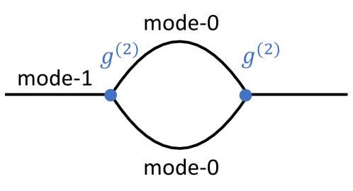
Figure 10: Feynman diagram for the self energy of mode-1 plasmon due to its parametric coupling to two mode-0 plasmons. Solid lines are the plasmon propagators.

In this subsection, we derive Eq. (9), the decay rate $\Gamma$ of the mode-1 plasmon into two mode-0 plasmons through the interaction Hamiltonian Eq. (7). This could be done by calculating the self energy (Fig. 10) of the mode-1 plasmon. It is a bubble diagram formed by two mode-0 propagators:

$$\Sigma(i\omega)= \left|\frac{g^{(2)}}{\hbar}\right|^{2}\sum_{q,i\Omega_{n}}\frac{\omega(q)}{(i\Omega_{n})^{2}-\omega(q)^{2}}\frac{\omega(q)}{(i\omega+i\Omega_{n})^{2}-\omega(q)^{2}}$$

$$= \left|\frac{g^{(2)}}{\hbar}\right|^{2}\sum_{q}\frac{\left[2n(\omega(q))+1\right]4\omega(q)}{(i\omega)^{2}-4\omega(q)^{2}}\,.$$ (94)

where $n(x)=1/(e^{\hbar x/T}-1)$ is the boson occupation number. Its imaginary part at $i\omega=\omega_{1}$ would simply give the Fermi’s golden rule:

$$\mathrm{Im}[\Sigma(\omega_{1})]= \left|\frac{g^{(2)}}{\hbar}\right|^{2}\sum_{q}\left[2n(\omega(q))+1\right]\pi\delta(\omega_{1}-2\omega(q))$$

$$= \left|\frac{g^{(2)}}{\hbar}\right|^{2}\frac{L}{v_{0}}\left(n(\omega_{1}/2)+\frac{1}{2}\right)\,$$ (95)

which is just Eq. (9).

Appendix D Classical parametric amplification via second-order nonlinearity

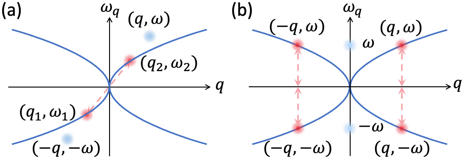
Figure 11: (a) Schematic illustration of 2D plasmons parametrically driven by the pump through second order nonlinearity. The blue curve is the plasmon frequency momentum dispersion. The red dots are the two plasmon modes coupled by the pump field at $(q,\omega)$ and its complex conjugate at $(-q,-\omega)$. (b) Degenerate FWM of plasmons induced by third order nonlinearity. The dots at zero momentum represent the uniform pump field with frequency $\omega$ and it complex conjugate. The dots at the same frequency but nonzero momentum represent the plasmon modes coupled by this field through third order nonlinearity.

D.1 Infinite plane

General—For the subharmonic generation to happen in inversion symmetric systems, there needs to be a strong pump field with frequency $\omega$ and appreciable wave vector $\mathbf{q}$ whose electric potential is

$$\Phi=\phi e^{i(\mathbf{q}\mathbf{r}-\omega t)}+\phi^{\ast}e^{-i(\mathbf{q}\mathbf{r}-\omega t)}\,.$$ (96)

The equation of motion (EOM) of the plasmons is conveniently described by the second order nonlinear conductivity

$$j_{\mu}(\omega,\mathbf{q}) =\int d\omega^{\prime}d\mathbf{q}^{\prime}\sigma_{\mu\alpha\beta}^{(2)}(\omega-\omega^{\prime},\mathbf{q}-\mathbf{q}^{\prime},\omega^{\prime},\mathbf{q}^{\prime})$$

$$E_{\alpha}(\omega-\omega^{\prime},\mathbf{q}-\mathbf{q}^{\prime})E_{\beta}(\omega^{\prime},\mathbf{q}^{\prime})\,.$$ (97)

Since $\sigma^{(2)}$ is a real function in space-time domain, its frequency momentum representation has the general property

$$\sigma_{\mu\alpha\beta}^{(2)}(-\omega_{1},-\mathbf{q}_{1},-\omega_{2},-\mathbf{q}_{2})=\sigma_{\mu\alpha\beta}^{{(2)}\ast}(\omega_{1},\mathbf{q}_{1},\omega_{2},\mathbf{q}_{2})\,.$$ (98)

And if the system has inversion symmetry, then

$$\sigma_{\mu\alpha\beta}^{(2)}(\omega_{1},-\mathbf{q}_{1},\omega_{2},-\mathbf{q}_{2})=-\sigma_{\mu\alpha\beta}^{(2)}(\omega_{1},\mathbf{q}_{1},\omega_{2},\mathbf{q}_{2})\,$$ (99)

which means $\sigma_{\mu\alpha\beta}^{(2)}(\omega_{1},0,\omega_{2},0)=0\,.$ However, it can be nonzero at finite momentum. By convention, $\sigma^{(2)}$ is defined to be symmetric: $\sigma_{\mu\alpha\beta}^{(2)}(\omega_{1},\mathbf{q}_{1},\omega_{2},\mathbf{q}_{2})=\sigma_{\mu\beta\alpha}^{(2)}(\omega_{2},\mathbf{q}_{2},\omega_{1},\mathbf{q}_{1})$.

Due to $\sigma^{(2)}$ and the driving field, the equation of motion for plasmons is modified. As illustrated in Fig. 11(a), any two modes $(\mathbf{q}_{1},\mathbf{q}_{2})$ with $\mathbf{q}_{1}+\mathbf{q}=\mathbf{q}_{2}$ are coupled by the driving field through $\sigma^{(2)}$. The charge continuity equation for the mode with momentum $\mathbf{q}_{2}$ is

$$\partial_{t}\rho_{\mathbf{q}_{2}}+\nabla\cdot\mathbf{j}_{\mathbf{q}_{2}}=0\,$$ (100)

and the current $\mathbf{j}_{\mathbf{q}_{2}}$ can be expanded to second order in electric field

$$j_{\mu}(\omega_{2},\mathbf{q}_{2})=\sigma_{\mu\nu}(\omega_{2},\mathbf{q}_{2})E^{\nu}(\omega_{2},\mathbf{q}_{2})+$$

$$\sigma_{\mu\alpha\beta}^{(2)}(\omega_{1},\mathbf{q}_{1},\omega,\mathbf{q})E^{\alpha}(\omega_{1},\mathbf{q}_{1})E^{\beta}(\omega,\mathbf{q})+$$

$$\sigma_{\mu\alpha\beta}^{(2)}(\omega,\mathbf{q},\omega_{1},\mathbf{q}_{1})E^{\alpha}(\omega,\mathbf{q})E^{\beta}(\omega_{1},\mathbf{q}_{1})\,.$$ (101)

The electric field $E(\omega_{2},\mathbf{q}_{2})$ is related to the charge density through the Coulomb kernel

$$\mathbf{E}(\omega_{2},\mathbf{q}_{2})=-i\mathbf{q}_{2}V_{q_{2}}\rho(\omega_{2},\mathbf{q}_{2})\,.$$ (102)

Similar set of equations apply to the pairing mode $\rho_{\mathbf{q}_{1}}$. Separating the densities into products of amplitude and phase as

$$\rho_{\mathbf{q}_{1}}=A_{1}(t)e^{i(\mathbf{q}_{1}\mathbf{r}-\omega_{1}t)},\quad\rho_{\mathbf{q}_{2}}=A_{2}(t)e^{i(\mathbf{q}_{2}\mathbf{r}-\omega_{2}t)}\,,$$ (103)

and plugging them into the continuity equations (Eq. (100) et al), we get the equations for time evolution equation of the amplitudes:

$$\begin{pmatrix}\partial_{t}+\gamma&&\kappa_{2}e^{i\Delta t}\\ \kappa_{1}e^{-i\Delta t}&&\partial_{t}+\gamma\end{pmatrix}\begin{pmatrix}A_{1}\\ A_{2}\end{pmatrix}=0\,.$$ (104)

The parameters $\kappa_{1}$, $\kappa_{2}$ are

$$\kappa_{1} =iq_{2\mu}\sigma_{\mu\alpha\beta}^{(2)}(\omega_{1},\mathbf{q}_{1},\omega,\mathbf{q})(-iq_{1\alpha}V_{q_{1}})(-iq_{\beta}\phi)$$

$$+iq_{2\mu}\sigma_{\mu\alpha\beta}^{(2)}(\omega,\mathbf{q},\omega_{1},\mathbf{q}_{1})(-iq_{\alpha}\phi)(-iq_{1\beta}V_{q_{1}})$$

$$=-i2\phi V_{q_{1}}\sigma_{\mu\alpha\beta}^{(2)}(\omega_{1},\mathbf{q}_{1},\omega,\mathbf{q})q_{2\mu}q_{1\alpha}q_{\beta}\,,$$

$$\kappa_{2} =i2\phi^{\ast}V_{q_{2}}\sigma_{\mu\alpha\beta}^{(2)}(\omega_{2},\mathbf{q}_{2},-\omega,-\mathbf{q})q_{1\mu}q_{2\alpha}q_{\beta}\,.$$ (105)

Simmilar to Eq. (45), the solution to Eq. (104) has an exponential factor $e^{\lambda t}$. For there to be nonzero solutions, we require the determinant to be zero, and obtain

$$\lambda=-\gamma\pm\sqrt{\kappa_{1}\kappa_{2}-\Delta^{2}/2}\,$$ (106)

where $\Delta=\omega-(\omega_{2}-\omega_{1})$. Therefore, the criterion for there to be an exponentially growing solution is

$$\mathrm{Re}\left[\sqrt{\kappa_{1}\kappa_{2}-\Delta^{2}/2}\right]>\gamma\,.$$ (107)

Let’s temporarily assume that there is no damping $\gamma=0$. In the ideal case, $\mathbf{q}_{1}=-\mathbf{q}_{2}$, and $\Delta=0$, we have $\kappa_{2}=\kappa^{\ast}_{1}$ from the property Eq. (98). Therefore, Eq. (107) is guaranteed to be satisfied in any dissipation-less system.

Applied to Graphene—In the kinetic regime of graphene, expanding to linear order in $q$, the second order nonlinear conductivity reads [20, 23]

$$\sigma^{(2)}_{ilm}(\omega_{1},\mathbf{q}_{1},\omega_{2},\mathbf{q}_{2})=\frac{D_{k}^{(2)}}{\omega_{1}\omega_{2}\omega_{3}}\Bigg{[}\left(q_{3}-\frac{\omega_{1}}{2\omega_{2}}q_{2}-\frac{\omega_{2}}{2\omega_{1}}q_{1}\right)_{i}\delta_{lm}+\left(2q_{2}-2q_{1}-\frac{\omega_{2}}{\omega_{1}}q_{1}+\frac{3\omega_{1}}{\omega_{2}}q_{2}\right)_{m}\delta_{il}\Bigg{]}+\left(\begin{smallmatrix}1&\leftrightarrow&2\\ l&\leftrightarrow&m\end{smallmatrix}\right)\,$$ (108)

where $(\omega_{3},\mathbf{q}_{3})=(\omega_{1}+\omega_{2},\mathbf{q}_{1}+\mathbf{q}_{2})$ and the second order optical weight is $D_{k}^{(2)}=D_{0}^{(2)}\tanh\left(\mu/(2T)\right)$ [23] whose zero temperature limit is $D^{(2)}_{0}$. Applied to Eq. (105) in the ideal case $\mathbf{q}_{1}=-\mathbf{q}_{2}$, and $\Delta=0$, we obtain the growth rate

$$\sqrt{\kappa_{1}\kappa_{2}}=\frac{3}{2}\frac{e^{3}v^{2}_{F}}{\hbar^{2}}\frac{q^{3}}{\omega^{3}}|\phi|\,.$$ (109)

Taking into account the plasmon dispersion $\omega_{1}=\sqrt{2Dq_{1}}$, we arrive at the dimensionless relative growth factor

$$Q_{g}^{-1}=\frac{3}{16\alpha_{g}}\zeta\,.$$ (110)

D.2 Graphene ribbon

Assume the $\omega_{1}$ mode is excited by an external source tuned exactly at $\omega_{1}$, the density is $\rho(t)=\rho_{0}e^{-i\omega_{1}t}+c.c.$. Through second order nonlinearity, the strong field of mode $\omega_{1}$ is going to modify the CCE of the $\omega_{0}$ mode. Assuming the charge density of the subharmonic mode is $\rho_{1}=A(t)e^{-i\omega_{0}t}+c.c.$, plugging it into the CCE of this mode and taking inner product with $\tilde{\rho}_{1}$, one obtains equation for the amplitude:

$$\partial_{t}A+\kappa A^{\ast}=0\,$$ (111)

where $|\tilde{\rho}_{1}|^{2}$ is defined in Eq. (69) and $|\kappa|=|\beta g/\hbar|$. Eq. (111) leads to exponentially growing solution with the relative growth rate

$$Q^{-1}_{g}=\frac{|\kappa|}{\omega_{0}}=\zeta\frac{Q}{8\alpha_{g}}\frac{\eta^{\prime}\alpha^{\prime}}{\xi^{2}_{0}S_{1}^{\prime}S_{0}^{\prime}}\,$$ (112)

which agrees with Eq. (17), the quantum mechanical result.

Appendix E Classical parametric amplification via third-order nonlinearity

Assume a strong uniform electric field $\mathbf{E}=\mathbf{E}_{0}e^{-i\omega t}+c.c.$ which, due to momentum mismatch, cannot excite plasmons through linear response. However, through third order nonlinear effect, this uniform $\mathbf{E}$ tends to make the plasmons grow in amplitude. The CCE of the plasmons with momentum $q$ is

$$\partial_{t}\rho_{\mathbf{q}}+\nabla\cdot\mathbf{j}_{\mathbf{q}}=0\,,$$ (113)

and the currents are

$$j(\mathbf{q},\omega)_{i}= \sigma_{il}(\omega)E(\mathbf{q},\omega)_{l}+$$

$$3\sigma^{(3)}_{ilmn}(-\omega,\omega,\omega)E(\mathbf{q},-\omega)_{l}E_{0m}E_{0n}\,,$$

$$j(\mathbf{q},-\omega)_{i}= \sigma_{il}(-\omega)E(\mathbf{q},-\omega)_{l}+$$

$$3\sigma^{(3)}_{ilmn}(\omega,-\omega,-\omega)E(\mathbf{q},\omega)_{l}E^{\ast}_{0m}E^{\ast}_{0n}$$ (114)

where $E(\mathbf{q})_{l}=-iq_{l}v_{q}\rho_{\mathbf{q}}$. Thus the CCEs of the plasmon mode $q$ at frequencies $\omega$ and $-\omega$ are coupled by the pump field $E_{0}$, as shown in Fig. 11(b). Separating amplitude and phase of the charge density as

$$\rho_{\mathbf{q}}(t)=A(t)e^{-i\omega t}+B(t)e^{i\omega t}\,$$ (115)

we arrive at the equation for the amplitudes

$$\begin{pmatrix}2\partial_{t}&&\lambda\\ \lambda^{\prime}&&2\partial_{t}\end{pmatrix}\begin{pmatrix}A\\ B\end{pmatrix}=0\,$$ (116)

where

$$\lambda =3\sigma^{(3)}_{ilmn}(-\omega,\omega,\omega)q_{i}q_{l}v_{q}E_{0m}E_{0n}\,,$$

$$\lambda^{\prime} =3\sigma^{(3)}_{ilmn}(\omega,-\omega,-\omega)q_{i}q_{l}v_{q}E^{\ast}_{0m}E^{\ast}_{0n}\,.$$ (117)

Due to the fact that $\sigma^{(3)}_{ilmn}(\omega,-\omega,-\omega)=\sigma^{(3)\ast}_{ilmn}(-\omega,\omega,\omega)$, we have $\lambda^{\prime}=\lambda^{\ast}$. Therefore, Eq. (116) has the solution

$$A(t) =A_{+}e^{\kappa t}+A_{-}e^{-\kappa t},$$

$$B(t) =B_{+}e^{\kappa t}+B_{-}e^{-\kappa t},$$ (118)

where $\kappa=|\lambda|$ is the growth/decay rate. Taking the ‘Drude’ form in Eq. (21) for $\sigma^{(3)}$ of graphene in the kinetic regime, plugging in the square root dispersion of plasmons $\omega=\sqrt{2Dq}$, the dimensionless relative growth rate $Q_{g}^{-1}=\kappa/\omega$ simplifies to

$$Q_{g}^{-1}=\frac{3}{8}\frac{e^{2}E^{2}_{0}/\omega^{2}}{(\hbar k_{F})^{2}}=\frac{3}{8}\xi^{2}$$ (119)

for the plasmons propagating parallel to the direction of the pump field. The dimensionless small number $\xi=\frac{eE_{0}/\omega}{\hbar k_{F}}=\delta p/p_{F}$ is simple to memorize: $\delta p$ is just the change in electron momentum caused by the electric field during one half cycle of the oscillations, $\delta t\sim\pi/\omega$ [24]. Note that due to third order nonlinearity, the plasmon frequency itself is also renormalized by this strong uniform field [24], and the frequency $\omega$ throughout this section should be considered as the renormalized one.

Although a result of third order nonlinearity, this phenomenon is different from modulational instability which is ubiquitous in nonlinear optics and fluid mechanics [131], e.g. in surface gravity waves. In modulational instability, the strong pump is a finite momentum ‘wave train’ on resonance, and the exponentially growing waves have momentums different from the pump by a small amount $\delta k$. If the criterion of instability is satisfied, the growth rate scales linearly with $\delta k$. For a negative Kerr nonlinearity as for graphene plasmons [24], the criterion requires $\partial^{2}_{k}\omega>0$, not satisfied by the square root dispersion. However, this criterion assumes a non dispersive $\sigma^{(3)}$ which is not true in graphene. Therefore, whether modulational instability happens in graphene needs further investigation and is a weaker effect anyway. Indeed, in a recent work on nonlinear plasmons [132], it was found that second order nonlinearity could lead to growth of side bands in the presence of a wave train, similar to modulational instability.

Appendix F Near-field probe of DFG

In this section, we discuss a scanning near field experiment that could measure plasmonic DFG by classical interference. The setup is similar to the left part of Fig. 6. Upon pumping of the $\omega_{1}$ mode of the device Fig. 1(a), if the $\omega_{0}$ mode with momentum $q$ is launched by a classical source combined with an ‘antenna’, e.g., the left edge of the ribbon, the counter propagating mode with momentum $-q$ will be generated by DFG from the pump and the $q$ mode. The $q$ mode can be described by a coherent state $|a_{0}\rangle$ which satisfies $a_{q}|a_{0}\rangle=a_{0}|a_{0}\rangle$. The Hamiltonian (7) leads to equation of motion for the $-q$ mode:

$$(\partial_{t}+\gamma)\langle a_{-q}\rangle=-i\omega_{0}\langle a_{-q}\rangle-ig^{(2)}\beta a_{0}^{\ast}e^{-i\omega_{0}t}/\hbar$$ (120)

where the phenomenological damping rate $\gamma$ has been added. After the driving term has been turned on for a time long enough, the steady state solution is

$$\langle a_{-q}\rangle=i\frac{g^{(2)}\beta}{\hbar\gamma}a_{0}^{\ast}e^{-i\omega_{0}t}=i\frac{\kappa}{\gamma}a_{0}^{\ast}e^{-i\omega_{0}t}\,.$$ (121)

Therefore, if the ‘reflection coefficient’ $\kappa/\gamma$ is at the order of one, the two waves would interfere to form fringes with period $\lambda_{0}/2$ where $\lambda_{0}=2\pi/q$ is the wavelength of the subharmonic plasmon. These fringes could be picked up by the near field scanning probe.

References

- Koppens et al. [2011] F. H. L. Koppens, D. E. Chang, and F. J. García de Abajo, Graphene plasmonics: A platform for strong light–matter interactions, Nano Letters 11, 3370 (2011).
- Basov et al. [2014] D. N. Basov, M. M. Fogler, A. Lanzara, F. Wang, and Y. Zhang, Colloquium: Graphene spectroscopy, Rev. Mod. Phys. 86, 959 (2014).
- Fei et al. [2012] Z. Fei, A. S. Rodin, G. O. Andreev, W. Bao, A. S. McLeod, M. Wagner, L. M. Zhang, Z. Zhao, M. Thiemens, G. Dominguez, M. M. Fogler, A. H. Castro Neto, C. N. Lau, F. Keilmann, and D. N. Basov, Gate-tuning of graphene plasmons revealed by infrared nano-imaging., Nature 487, 82 (2012).
- Chen et al. [2012] J. Chen, M. Badioli, P. Alonso-González, S. Thongrattanasiri, F. Huth, J. Osmond, M. Spasenović, A. Centeno, A. Pesquera, P. Godignon, A. Zurutuza Elorza, N. Camara, F. J. G. de Abajo, R. Hillenbrand, and F. H. L. Koppens, Optical nano-imaging of gate-tunable graphene plasmons, Nature 487, 77 (2012).
- Woessner et al. [2015] A. Woessner, M. B. Lundeberg, Y. Gao, A. Principi, P. Alonso-Gonzalez, M. Carrega, K. Watanabe, T. Taniguchi, G. Vignale, M. Polini, J. Hone, R. Hillenbrand, and F. H. L. Koppens, Highly confined low-loss plasmons in graphene-boron nitride heterostructures, Nature Materials 14, 421 (2015).
- Shi et al. [2015] Z. Shi, X. Hong, H. A. Bechtel, B. Zeng, M. C. Martin, K. Watanabe, T. Taniguchi, Y.-R. Shen, and F. Wang, Observation of a luttinger-liquid plasmon in metallic single-walled carbon nanotubes, Nature Photonics 9, 515 (2015).
- Ni et al. [2016] G. X. Ni, L. Wang, M. D. Goldflam, M. Wagner, Z. Fei, A. S. McLeod, M. K. Liu, F. Keilmann, B. Özyilmaz, A. H. Castro Neto, J. Hone, M. M. Fogler, and D. N. Basov, Ultrafast optical switching of infrared plasmon polaritons in high-mobility graphene, Nature Photonics 10, 244 (2016).
- Lundeberg et al. [2017] M. B. Lundeberg, Y. Gao, R. Asgari, C. Tan, B. Van Duppen, M. Autore, P. Alonso-González, A. Woessner, K. Watanabe, T. Taniguchi, R. Hillenbrand, J. Hone, M. Polini, and F. H. L. Koppens, Tuning quantum nonlocal effects in graphene plasmonics., Science 357, 187 (2017).
- Ni et al. [2018] G. X. Ni, A. S. McLeod, Z. Sun, L. Wang, L. Xiong, K. W. Post, S. S. Sunku, B.-Y. Jiang, J. Hone, C. R. Dean, M. M. Fogler, and D. N. Basov, Fundamental limits to graphene plasmonics, Nature 557, 530 (2018).
- Wang et al. [2020] S. Wang, S. Zhao, Z. Shi, F. Wu, Z. Zhao, L. Jiang, K. Watanabe, T. Taniguchi, A. Zettl, C. Zhou, and F. Wang, Nonlinear luttinger liquid plasmons in semiconducting single-walled carbon nanotubes, Nature Materials 19, 986 (2020).
- Dong et al. [2021] Y. Dong, L. Xiong, I. Y. Phinney, Z. Sun, R. Jing, A. S. McLeod, S. Zhang, S. Liu, F. L. Ruta, H. Gao, Z. Dong, R. Pan, J. H. Edgar, P. Jarillo-Herrero, L. S. Levitov, A. J. Millis, M. M. Fogler, D. A. Bandurin, and D. N. Basov, Fizeau drag in graphene plasmonics, Nature 594, 513 (2021).
- Zhao et al. [2021] W. Zhao, S. Zhao, H. Li, S. Wang, S. Wang, M. I. B. Utama, S. Kahn, Y. Jiang, X. Xiao, S. Yoo, K. Watanabe, T. Taniguchi, A. Zettl, and F. Wang, Efficient fizeau drag from dirac electrons in monolayer graphene, Nature 594, 517 (2021).
- Wang et al. [2021] S. Wang, S. Yoo, S. Zhao, W. Zhao, S. Kahn, D. Cui, F. Wu, L. Jiang, M. I. B. Utama, H. Li, S. Li, A. Zibrov, E. Regan, D. Wang, Z. Zhang, K. Watanabe, T. Taniguchi, C. Zhou, and F. Wang, Gate-tunable plasmons in mixed-dimensional van der waals heterostructures, Nature Communications 12, 5039 (2021).
- Hu et al. [2022] H. Hu, R. Yu, H. Teng, D. Hu, N. Chen, Y. Qu, X. Yang, X. Chen, A. S. McLeod, P. Alonso-González, X. Guo, C. Li, Z. Yao, Z. Li, J. Chen, Z. Sun, M. Liu, F. J. García de Abajo, and Q. Dai, Active control of micrometer plasmon propagation in suspended graphene, Nature Communications 13, 1465 (2022).
- Mikhailov [2007] S. A. Mikhailov, Non-linear electromagnetic response of graphene, Europhys. Lett. 79, 27002 (2007).
- Mikhailov [2011] S. A. Mikhailov, Theory of the giant plasmon-enhanced second-harmonic generation in graphene and semiconductor two-dimensional electron systems, Phys. Rev. B 84, 045432 (2011).
- Manzoni et al. [2015] M. T. Manzoni, I. Silveiro, F. J. G. D. Abajo, and D. E. Chang, Second-order quantum nonlinear optical processes in single graphene nanostructures and arrays, New J. Phys. 17, 83031 (2015).
- Glazov and Ganichev [2014] M. Glazov and S. Ganichev, High frequency electric field induced nonlinear effects in graphene, Phys. Rep. 535, 101 (2014).
- Cheng et al. [2014] J. L. Cheng, N. Vermeulen, and J. E. Sipe, Third order optical nonlinearity of graphene, New J. Phys. 16, 053014 (2014).
- Wang et al. [2016] Y. Wang, M. Tokman, and A. Belyanin, Second-order nonlinear optical response of graphene, Phys. Rev. B 94, 195442 (2016).
- Mikhailov [2017a] S. A. Mikhailov, Influence of optical nonlinearities on plasma waves in graphene, ACS Photonics 4, 3018 (2017a).
- Mikhailov [2017b] S. A. Mikhailov, Nonperturbative quasiclassical theory of the nonlinear electrodynamic response of graphene, Phys. Rev. B 95, 085432 (2017b).
- Sun et al. [2018a] Z. Sun, D. N. Basov, and M. M. Fogler, Universal linear and nonlinear electrodynamics of a dirac fluid, Proceedings of the National Academy of Sciences 115, 3285 (2018a).
- Sun et al. [2018b] Z. Sun, D. N. Basov, and M. M. Fogler, Third-order optical conductivity of an electron fluid, Phys. Rev. B 97, 075432 (2018b).
- Constant et al. [2015] T. J. Constant, S. M. Hornett, D. E. Chang, and E. Hendry, All-optical generation of surface plasmons in graphene, Nat. Phys. 12, 124 (2015).
- Yao et al. [2018] B. Yao, Y. Liu, S.-W. Huang, C. Choi, Z. Xie, J. Flor Flores, Y. Wu, M. Yu, D.-L. Kwong, Y. Huang, Y. Rao, X. Duan, and C. W. Wong, Broadband gate-tunable terahertz plasmons in graphene heterostructures, Nature Photonics 12, 22 (2018).
- Kroo et al. [2008] N. Kroo, S. Varró, G. Farkas, P. Dombi, D. Oszetzky, A. Nagy, and A. Czitrovszky, Nonlinear plasmonics, Journal of Modern Optics 55, 3203 (2008).
- Gullans et al. [2013] M. Gullans, D. E. Chang, F. H. L. Koppens, F. J. G. de Abajo, and M. D. Lukin, Single-photon nonlinear optics with graphene plasmons, Phys. Rev. Lett. 111, 247401 (2013).
- Kauranen and Zayats [2012] M. Kauranen and A. V. Zayats, Nonlinear plasmonics, Nature Photonics 6, 737 (2012).
- Cox et al. [2017] J. D. Cox, A. Marini, and F. J. G. de Abajo, Plasmon-assisted high-harmonic generation in graphene, Nature Communications 8, 14380 (2017).
- Tame et al. [2013] M. S. Tame, K. R. McEnery, c. K. Özdemir, J. Lee, S. A. Maier, and M. S. Kim, Quantum plasmonics, Nat. Phys. 9, 329 (2013).
- Reserbat-Plantey et al. [2021] A. Reserbat-Plantey, I. Epstein, I. Torre, A. T. Costa, P. A. D. Gonçalves, N. A. Mortensen, M. Polini, J. C. W. Song, N. M. R. Peres, and F. H. L. Koppens, Quantum nanophotonics in two-dimensional materials, ACS Photonics 8, 85 (2021).
- Boyd [2020] R. W. Boyd, Nonlinear optics (Elsevier Science, Amsterdam, Netherlands, 2020).
- Reid et al. [2009] M. D. Reid, P. D. Drummond, W. P. Bowen, E. G. Cavalcanti, P. K. Lam, H. A. Bachor, U. L. Andersen, and G. Leuchs, Colloquium: The Einstein-Podolsky-Rosen paradox: From concepts to applications, Rev. Mod. Phys. 81, 1727 (2009).
- Pan et al. [2012] J.-W. Pan, Z.-B. Chen, C.-Y. Lu, H. Weinfurter, A. Zeilinger, and M. Żukowski, Multiphoton entanglement and interferometry, Rev. Mod. Phys. 84, 777 (2012).
- Orieux et al. [2017] A. Orieux, M. A. M. Versteegh, K. D. Jöns, and S. Ducci, Semiconductor devices for entangled photon pair generation: a review, Reports on Progress in Physics 80, 076001 (2017).
- Kwiat et al. [1995] P. G. Kwiat, K. Mattle, H. Weinfurter, A. Zeilinger, A. V. Sergienko, and Y. Shih, New high-intensity source of polarization-entangled photon pairs, Phys. Rev. Lett. 75, 4337 (1995).
- Wang et al. [2019] H. Wang, H. Hu, T.-H. Chung, J. Qin, X. Yang, J.-P. Li, R.-Z. Liu, H.-S. Zhong, Y.-M. He, X. Ding, Y.-H. Deng, Q. Dai, Y.-H. Huo, S. Höfling, C.-Y. Lu, and J.-W. Pan, On-demand semiconductor source of entangled photons which simultaneously has high fidelity, efficiency, and indistinguishability, Phys. Rev. Lett. 122, 113602 (2019).
- De Rossi and Berger [2002] A. De Rossi and V. Berger, Counterpropagating twin photons by parametric fluorescence, Phys. Rev. Lett. 88, 043901 (2002).
- Steiner et al. [2021] T. J. Steiner, J. E. Castro, L. Chang, Q. Dang, W. Xie, J. Norman, J. E. Bowers, and G. Moody, Ultrabright entangled-photon-pair generation from an -on-insulator microring resonator, PRX Quantum 2, 010337 (2021).
- Javid et al. [2021] U. A. Javid, J. Ling, J. Staffa, M. Li, Y. He, and Q. Lin, Ultrabroadband entangled photons on a nanophotonic chip, Phys. Rev. Lett. 127, 183601 (2021).
- Zhang and Fogler [2008] L. M. Zhang and M. M. Fogler, Nonlinear screening and ballistic transport in a graphene junction, Phys. Rev. Lett. 100, 116804 (2008).
- Vicarelli et al. [2012] L. Vicarelli, M. S. Vitiello, D. Coquillat, A. Lombardo, A. C. Ferrari, W. Knap, M. Polini, V. Pellegrini, and A. Tredicucci, Graphene field-effect transistors as room-temperature terahertz detectors, Nature Materials 11, 865 (2012).
- Woessner et al. [2017] A. Woessner, R. Parret, D. Davydovskaya, Y. Gao, J.-S. Wu, M. B. Lundeberg, S. Nanot, P. Alonso-Gonzalez, K. Watanabe, T. Taniguchi, R. Hillenbrand, M. M. Fogler, J. Hone, and F. H. L. Koppens, Electrical detection of hyperbolic phonon-polaritons in heterostructures of graphene and boron nitride, npj 2D Mater. Appl. 1, 25 (2017).
- Alonso-González et al. [2017] P. Alonso-González, A. Y. Nikitin, Y. Gao, A. Woessner, M. B. Lundeberg, A. Principi, N. Forcellini, W. Yan, S. Vélez, A. J. Huber, K. Watanabe, T. Taniguchi, F. Casanova, L. E. Hueso, M. Polini, J. Hone, F. H. L. Koppens, and R. Hillenbrand, Acoustic terahertz graphene plasmons revealed by photocurrent nanoscopy, Nature Nanotechnology 12, 31 (2017).
- Castilla et al. [2019] S. Castilla, B. Terrés, M. Autore, L. Viti, J. Li, A. Y. Nikitin, I. Vangelidis, K. Watanabe, T. Taniguchi, E. Lidorikis, M. S. Vitiello, R. Hillenbrand, K.-J. Tielrooij, and F. H. L. Koppens, Fast and sensitive terahertz detection using an antenna-integrated graphene pn junction, Nano Letters 19, 2765 (2019).
- Ding et al. [1995] Y. J. Ding, S. J. Lee, and J. B. Khurgin, Transversely pumped counterpropagating optical parametric oscillation and amplification, Phys. Rev. Lett. 75, 429 (1995).
- Saravi et al. [2017] S. Saravi, T. Pertsch, and F. Setzpfandt, Generation of counterpropagating path-entangled photon pairs in a single periodic waveguide, Phys. Rev. Lett. 118, 183603 (2017).
- Jiang et al. [2018a] B.-Y. Jiang, E. J. Mele, and M. M. Fogler, Theory of plasmon reflection by a 1d junction, Opt. Express 26, 17209 (2018a).
- Wolff and Mortensen [2020] C. Wolff and N. A. Mortensen, Stimulated plasmon polariton scattering, Nature communications 11, 4039 (2020).
- Tokman et al. [2016] M. Tokman, Y. Wang, I. Oladyshkin, A. R. Kutayiah, and A. Belyanin, Laser-driven parametric instability and generation of entangled photon-plasmon states in graphene, Phys. Rev. B 93, 235422 (2016).
- Mishchenko et al. [2010] E. G. Mishchenko, A. V. Shytov, and P. G. Silvestrov, Guided plasmons in graphene junctions, Phys. Rev. Lett. 104, 156806 (2010).
- Hu et al. [2017] F. Hu, Y. Luan, Z. Fei, I. Z. Palubski, M. D. Goldflam, S. Dai, J. S. Wu, K. W. Post, G. C. A. M. Janssen, M. M. Fogler, and D. N. Basov, Imaging the localized plasmon resonance modes in graphene nanoribbons, Nano Letters 17, 5423 (2017).
- Cheng et al. [2017] J. L. Cheng, N. Vermeulen, and J. E. Sipe, Second order optical nonlinearity of graphene due to electric quadrupole and magnetic dipole effects, Sci. Rep. 7, 43843 (2017).
- Orieux et al. [2011] A. Orieux, X. Caillet, A. Lemaître, P. Filloux, I. Favero, G. Leo, and S. Ducci, Efficient parametric generation of counterpropagating two-photon states, J. Opt. Soc. Am. B 28, 45 (2011).
- Yan et al. [2013] H. Yan, T. Low, W. Zhu, Y. Wu, M. Freitag, X. Li, F. Guinea, P. Avouris, and F. Xia, Damping pathways of mid-infrared plasmons in graphene nanostructures, Nature Photonics 7, 394 (2013).
- Caves and Schumaker [1985] C. M. Caves and B. L. Schumaker, New formalism for two-photon quantum optics. I. Quadrature phases and squeezed states, Phys. Rev. A 31, 3068 (1985).
- Martin et al. [2017] A. Martin, T. Guerreiro, A. Tiranov, S. Designolle, F. Fröwis, N. Brunner, M. Huber, and N. Gisin, Quantifying photonic high-dimensional entanglement, Phys. Rev. Lett. 118, 110501 (2017).
- Lee et al. [2020a] G.-H. Lee, D. K. Efetov, W. Jung, L. Ranzani, E. D. Walsh, T. A. Ohki, T. Taniguchi, K. Watanabe, P. Kim, D. Englund, and K. C. Fong, Graphene-based josephson junction microwave bolometer, Nature 586, 42 (2020a).
- Howell et al. [2004] J. C. Howell, R. S. Bennink, S. J. Bentley, and R. W. Boyd, Realization of the einstein-podolsky-rosen paradox using momentum- and position-entangled photons from spontaneous parametric down conversion, Phys. Rev. Lett. 92, 210403 (2004).
- MacLean et al. [2018] J.-P. W. MacLean, J. M. Donohue, and K. J. Resch, Direct characterization of ultrafast energy-time entangled photon pairs, Phys. Rev. Lett. 120, 053601 (2018).
- Franson [1989] J. D. Franson, Bell inequality for position and time, Phys. Rev. Lett. 62, 2205 (1989).
- Fasel et al. [2005] S. Fasel, F. Robin, E. Moreno, D. Erni, N. Gisin, and H. Zbinden, Energy-time entanglement preservation in plasmon-assisted light transmission, Phys. Rev. Lett. 94, 110501 (2005).
- Soavi et al. [2018] G. Soavi, G. Wang, H. Rostami, D. G. Purdie, D. De Fazio, T. Ma, B. Luo, J. Wang, A. K. Ott, D. Yoon, S. A. Bourelle, J. E. Muench, I. Goykhman, S. Dal Conte, M. Celebrano, A. Tomadin, M. Polini, G. Cerullo, and A. C. Ferrari, Broadband, electrically tunable third-harmonic generation in graphene, Nature Nanotechnology 13, 583 (2018).
- Jiang et al. [2018b] T. Jiang, D. Huang, J. Cheng, X. Fan, Z. Zhang, Y. Shan, Y. Yi, Y. Dai, L. Shi, K. Liu, C. Zeng, J. Zi, J. E. Sipe, Y.-R. Shen, W.-T. Liu, and S. Wu, Gate-tunable third-order nonlinear optical response of massless dirac fermions in graphene, Nature Photonics 12, 430 (2018b).
- Mikhailov [2016] S. A. Mikhailov, Quantum theory of the third-order nonlinear electrodynamic effects of graphene, Phys. Rev. B 93, 085403 (2016).
- Absil et al. [2000] P. P. Absil, J. V. Hryniewicz, B. E. Little, P. S. Cho, R. A. Wilson, L. G. Joneckis, and P.-T. Ho, Wavelength conversion in gaas micro-ring resonators, Opt. Lett. 25, 554 (2000).
- Helt et al. [2010] L. G. Helt, Z. Yang, M. Liscidini, and J. E. Sipe, Spontaneous four-wave mixing in microring resonators, Opt. Lett. 35, 3006 (2010).
- Ferrera et al. [2008] M. Ferrera, L. Razzari, D. Duchesne, R. Morandotti, Z. Yang, M. Liscidini, J. E. Sipe, S. Chu, B. E. Little, and D. J. Moss, Low-power continuous-wave nonlinear optics in doped silica glass integrated waveguide structures, Nature Photonics 2, 737 (2008).
- Levy et al. [2010] J. S. Levy, A. Gondarenko, M. A. Foster, A. C. Turner-Foster, A. L. Gaeta, and M. Lipson, Cmos-compatible multiple-wavelength oscillator for on-chip optical interconnects, Nature Photonics 4, 37 (2010).
- Sirtori et al. [1994] C. Sirtori, F. Capasso, J. Faist, L. N. Pfeiffer, and K. W. West, Far‐infrared generation by doubly resonant difference frequency mixing in a coupled quantum well two‐dimensional electron gas system, Applied Physics Letters 65, 445 (1994).
- Belkin et al. [2007] M. A. Belkin, F. Capasso, A. Belyanin, D. L. Sivco, A. Y. Cho, D. C. Oakley, C. J. Vineis, and G. W. Turner, Terahertz quantum-cascade-laser source based on intracavity difference-frequency generation, Nature Photonics 1, 288 (2007).
- Zhao et al. [2020] J. Zhao, C. Ma, M. Rüsing, and S. Mookherjea, High quality entangled photon pair generation in periodically poled thin-film lithium niobate waveguides, Phys. Rev. Lett. 124, 163603 (2020).
- Guo et al. [2017] X. Guo, C.-l. Zou, C. Schuck, H. Jung, R. Cheng, and H. X. Tang, Parametric down-conversion photon-pair source on a nanophotonic chip, Light: Science & Applications 6, e16249 (2017).
- Koos et al. [2007] C. Koos, L. Jacome, C. Poulton, J. Leuthold, and W. Freude, Nonlinear silicon-on-insulator waveguides for all-optical signal processing, Opt. Express 15, 5976 (2007).
- Ma et al. [2017] C. Ma, X. Wang, V. Anant, A. D. Beyer, M. D. Shaw, and S. Mookherjea, Silicon photonic entangled photon-pair and heralded single photon generation with CAR12,000 and , Opt. Express 25, 32995 (2017).
- [77] R. R. Kumar, M. Raevskaia, V. Pogoretskii, Y. Jiao, and H. K. Tsang, Entangled photon pair generation from an inp membrane micro-ring resonator, Applied Physics Letters 114, 021104.
- Ramelow et al. [2015] S. Ramelow, A. Farsi, S. Clemmen, D. Orquiza, K. Luke, M. Lipson, and A. L. Gaeta, Silicon-nitride platform for narrowband entangled photon generation (2015), arXiv:1508.04358 [quant-ph] .
- Alonso Calafell et al. [2019] I. Alonso Calafell, J. D. Cox, M. Radonjić, J. R. M. Saavedra, F. J. García de Abajo, L. A. Rozema, and P. Walther, Quantum computing with graphene plasmons, npj Quantum Information 5, 37 (2019).
- Page et al. [2015] A. F. Page, F. Ballout, O. Hess, and J. M. Hamm, Nonequilibrium plasmons with gain in graphene, Phys. Rev. B 91, 075404 (2015).
- Sun et al. [2016] Z. Sun, D. N. Basov, and M. M. Fogler, Adiabatic Amplification of Plasmons and Demons in 2D Systems, Phys. Rev. Lett. 117, 076805 (2016).
- de Vega and García de Abajo [2017] S. de Vega and F. J. García de Abajo, Plasmon generation through electron tunneling in graphene, ACS Photonics, ACS Photonics 4, 2367 (2017).
- Wilson et al. [2018] J. Wilson, F. Santosa, M. Min, and T. Low, Temporal control of graphene plasmons, Phys. Rev. B 98, 081411(R) (2018).
- Rajasekaran et al. [2016] S. Rajasekaran, E. Casandruc, Y. Laplace, D. Nicoletti, G. D. Gu, S. R. Clark, D. Jaksch, and A. Cavalleri, Parametric amplification of a superconducting plasma wave, Nat. Phys. 12, 1012 (2016).
- Moreau et al. [2019] P.-A. Moreau, E. Toninelli, T. Gregory, and M. J. Padgett, Imaging with quantum states of light, Nature Reviews Physics 1, 367 (2019).
- Pirandola et al. [2018] S. Pirandola, B. R. Bardhan, T. Gehring, C. Weedbrook, and S. Lloyd, Advances in photonic quantum sensing, Nature Photonics 12, 724 (2018).
- Yao et al. [2014] X. Yao, M. Tokman, and A. Belyanin, Efficient Nonlinear Generation of THz Plasmons in Graphene and Topological Insulators, Phys. Rev. Lett. 112, 055501 (2014).
- Rostami et al. [2017] H. Rostami, M. I. Katsnelson, and M. Polini, Theory of plasmonic effects in nonlinear optics: The case of graphene, Phys. Rev. B 95, 035416 (2017).
- Wolff et al. [2019] C. Wolff, C. Tserkezis, and N. A. Mortensen, Enhanced ponderomotive force in graphene due to interband resonance, New Journal of Physics 21, 073046 (2019).
- Tollerton et al. [2019] C. J. Tollerton, J. Bohn, T. J. Constant, S. A. R. Horsley, D. E. Chang, E. Hendry, and D. Z. Li, Origins of all-optical generation of plasmons in graphene, Scientific Reports 9, 3267 (2019).
- Altewischer et al. [2002] E. Altewischer, M. P. van Exter, and J. P. Woerdman, Plasmon-assisted transmission of entangled photons, Nature 418, 304 (2002).
- Phan et al. [2013] T. V. Phan, J. C. W. Song, and L. S. Levitov, Ballistic heat transfer and energy waves in an electron system (2013), arXiv:1306.4972 [cond-mat.mes-hall] .
- Svintsov [2018] D. Svintsov, Hydrodynamic-to-ballistic crossover in dirac materials, Phys. Rev. B 97, 121405(R) (2018).
- Lucas and Das Sarma [2018] A. Lucas and S. Das Sarma, Electronic sound modes and plasmons in hydrodynamic two-dimensional metals, Phys. Rev. B 97, 115449 (2018).
- Patrick et al. [2019] G. Patrick, Y. Chan-Shan, L. Tairu, T. Fanglin, K. Rai, Z. Hai, W. Kenji, T. Takashi, and W. Feng, Quantum-critical conductivity of the dirac fluid in graphene, Science 364, 158 (2019).
- Andreeva et al. [2020] V. Andreeva, D. A. Bandurin, M. Luskin, and D. Margetis, Dipole excitation of collective modes in viscous two-dimensional electron systems, Phys. Rev. B 102, 205411 (2020).
- Narozhny et al. [2021] B. N. Narozhny, I. V. Gornyi, and M. Titov, Hydrodynamic collective modes in graphene, Phys. Rev. B 103, 115402 (2021).
- Levchenko and Schmalian [2020] A. Levchenko and J. Schmalian, Transport properties of strongly coupled electron–phonon liquids, Annals of Physics 419, 168218 (2020).
- Principi et al. [2019] A. Principi, D. Bandurin, H. Rostami, and M. Polini, Pseudo-euler equations from nonlinear optics: Plasmon-assisted photodetection beyond hydrodynamics, Phys. Rev. B 99, 075410 (2019).
- Svintsov et al. [2013] D. Svintsov, V. Vyurkov, V. Ryzhii, and T. Otsuji, Hydrodynamic electron transport and nonlinear waves in graphene, Phys. Rev. B 88, 245444 (2013).
- Basov et al. [2016] D. N. Basov, M. M. Fogler, and F. J. García de Abajo, Polaritons in van der waals materials, Science 354, 195 (2016).
- Low et al. [2017] T. Low, A. Chaves, J. D. Caldwell, A. Kumar, N. X. Fang, P. Avouris, T. F. Heinz, F. Guinea, L. Martin-Moreno, and F. Koppens, Polaritons in layered two-dimensional materials, Nature Materials 16, 182 (2017).
- Basov et al. [2021] D. N. Basov, A. Asenjo-Garcia, P. J. Schuck, X. Zhu, and A. Rubio, Polariton panorama, Nanophotonics 10, 549 (2021).
- Dai et al. [2019] S. Dai, W. Fang, N. Rivera, Y. Stehle, B.-Y. Jiang, J. Shen, R. Y. Tay, C. J. Ciccarino, Q. Ma, D. Rodan-Legrain, P. Jarillo-Herrero, E. H. T. Teo, M. M. Fogler, P. Narang, J. Kong, and D. N. Basov, Phonon polaritons in monolayers of hexagonal boron nitride, Advanced Materials 31, 1806603 (2019).
- Li et al. [2021] N. Li, X. Guo, X. Yang, R. Qi, T. Qiao, Y. Li, R. Shi, Y. Li, K. Liu, Z. Xu, L. Liu, F. J. García de Abajo, Q. Dai, E.-G. Wang, and P. Gao, Direct observation of highly confined phonon polaritons in suspended monolayer hexagonal boron nitride, Nature Materials 20, 43 (2021).
- Dai et al. [2014] S. Dai, Z. Fei, Q. Ma, A. S. Rodin, M. Wagner, A. S. McLeod, M. K. Liu, W. Gannett, W. Regan, K. Watanabe, T. Taniguchi, M. Thiemens, G. Dominguez, A. H. C. Neto, A. Zettl, F. Keilmann, P. Jarillo-Herrero, M. M. Fogler, and D. N. Basov, Tunable Phonon Polaritons in Atomically Thin van der Waals Crystals of Boron Nitride, Science 343, 1125 (2014).
- Yoxall et al. [2015] E. Yoxall, M. Schnell, A. Y. Nikitin, O. Txoperena, A. Woessner, M. B. Lundeberg, F. Casanova, L. E. Hueso, F. H. L. Koppens, and R. Hillenbrand, Direct observation of ultraslow hyperbolic polariton propagation with negative phase velocity, Nature Photonics 9, 674 (2015).
- Li et al. [2015] P. Li, M. Lewin, A. V. Kretinin, J. D. Caldwell, K. S. Novoselov, T. Taniguchi, K. Watanabe, F. Gaussmann, and T. Taubner, Hyperbolic phonon-polaritons in boron nitride for near-field optical imaging and focusing, Nature Communications 6, 7507 (2015).
- Sun et al. [2015] Z. Sun, Á. Gutiérrez-Rubio, D. N. Basov, and M. M. Fogler, Hamiltonian optics of hyperbolic polaritons in nanogranules, Nano Letters 15, 4455 (2015).
- Rivera et al. [2017] N. Rivera, G. Rosolen, J. D. Joannopoulos, I. Kaminer, and M. Soljačić, Making two-photon processes dominate one-photon processes using mid-ir phonon polaritons, Proceedings of the National Academy of Sciences 114, 13607 (2017).
- Giles et al. [2018] A. J. Giles, S. Dai, I. Vurgaftman, T. Hoffman, S. Liu, L. Lindsay, C. T. Ellis, N. Assefa, I. Chatzakis, T. L. Reinecke, J. G. Tischler, M. M. Fogler, J. H. Edgar, D. N. Basov, and J. D. Caldwell, Ultralow-loss polaritons in isotopically pure boron nitride, Nat. Mater. 17, 134 (2018).
- Brown et al. [2018] L. V. Brown, M. Davanco, Z. Sun, A. Kretinin, Y. Chen, J. R. Matson, I. Vurgaftman, N. Sharac, A. J. Giles, M. M. Fogler, T. Taniguchi, K. Watanabe, K. S. Novoselov, S. A. Maier, A. Centrone, and J. D. Caldwell, Nanoscale Mapping and Spectroscopy of Nonradiative Hyperbolic Modes in Hexagonal Boron Nitride Nanostructures, Nano Lett. 18, 1628 (2018).
- Lee et al. [2020b] I.-H. Lee, M. He, X. Zhang, Y. Luo, S. Liu, J. H. Edgar, K. Wang, P. Avouris, T. Low, J. D. Caldwell, and S.-H. Oh, Image polaritons in boron nitride for extreme polariton confinement with low losses, Nature Communications 11, 3649 (2020b).
- Ni et al. [2021] G. Ni, A. S. McLeod, Z. Sun, J. R. Matson, C. F. B. Lo, D. A. Rhodes, F. L. Ruta, S. L. Moore, R. A. Vitalone, R. Cusco, L. Artús, L. Xiong, C. R. Dean, J. C. Hone, A. J. Millis, M. M. Fogler, J. H. Edgar, J. D. Caldwell, and D. N. Basov, Long-lived phonon polaritons in hyperbolic materials, Nano Letters 21, 5767 (2021).
- Moore et al. [2021] S. L. Moore, C. J. Ciccarino, D. Halbertal, L. J. McGilly, N. R. Finney, K. Yao, Y. Shao, G. Ni, A. Sternbach, E. J. Telford, B. S. Kim, S. E. Rossi, K. Watanabe, T. Taniguchi, A. N. Pasupathy, C. R. Dean, J. Hone, P. J. Schuck, P. Narang, and D. N. Basov, Nanoscale lattice dynamics in hexagonal boron nitride moirésuperlattices, Nature Communications 12, 5741 (2021).
- Cartella et al. [2018] A. Cartella, T. F. Nova, M. Fechner, R. Merlin, and A. Cavalleri, Parametric amplification of optical phonons, Proceedings of the National Academy of Sciences 115, 12148 (2018).
- Michael et al. [2020] M. H. Michael, A. von Hoegen, M. Fechner, M. Först, A. Cavalleri, and E. Demler, Parametric resonance of Josephson plasma waves: A theory for optically amplified interlayer superconductivity in , Phys. Rev. B 102, 174505 (2020).
- Sun et al. [2020] Z. Sun, M. M. Fogler, D. N. Basov, and A. J. Millis, Collective modes and terahertz near-field response of superconductors, Phys. Rev. Research 2, 023413 (2020).
- Dolgirev et al. [2021] P. E. Dolgirev, A. Zong, M. H. Michael, J. B. Curtis, D. Podolsky, A. Cavalleri, and E. Demler, Periodic dynamics in superconductors induced by an impulsive optical quench (2021), arXiv:2104.07181 [cond-mat.supr-con] .
- Golež et al. [2020] D. Golež, Z. Sun, Y. Murakami, A. Georges, and A. J. Millis, Nonlinear spectroscopy of collective modes in an excitonic insulator, Phys. Rev. Lett. 125, 257601 (2020).
- Sun and Millis [2020] Z. Sun and A. J. Millis, Bardasis-schrieffer polaritons in excitonic insulators, Phys. Rev. B 102, 041110(R) (2020).
- Murakami et al. [2020] Y. Murakami, D. Golež, T. Kaneko, A. Koga, A. J. Millis, and P. Werner, Collective modes in excitonic insulators: Effects of electron-phonon coupling and signatures in the optical response, Phys. Rev. B 101, 195118 (2020).
- Kaneko et al. [2021] T. Kaneko, Z. Sun, Y. Murakami, D. Golež, and A. J. Millis, Bulk photovoltaic effect driven by collective excitations in a correlated insulator, Phys. Rev. Lett. 127, 127402 (2021).
- Sun et al. [2021] Z. Sun, T. Kaneko, D. Golež, and A. J. Millis, Second-order josephson effect in excitonic insulators, Phys. Rev. Lett. 127, 127702 (2021).
- [125] E. W. Weisstein, Mathieu function, from MathWorld–A Wolfram Web Resource.
- García De Abajo [2007] F. J. García De Abajo, Colloquium: Light scattering by particle and hole arrays, Rev. Mod. Phys. 79, 1267 (2007).
- Wang et al. [2015] W. Wang, T. Christensen, A.-P. Jauho, K. S. Thygesen, M. Wubs, and N. A. Mortensen, Plasmonic eigenmodes in individual and bow-tie graphene nanotriangles, Scientific Reports 5, 9535 (2015).
- Franke et al. [2019] S. Franke, S. Hughes, M. K. Dezfouli, P. T. Kristensen, K. Busch, A. Knorr, and M. Richter, Quantization of quasinormal modes for open cavities and plasmonic cavity quantum electrodynamics, Phys. Rev. Lett. 122, 213901 (2019).
- Ren et al. [2021] J. Ren, S. Franke, and S. Hughes, Quasinormal modes, local density of states, and classical purcell factors for coupled loss-gain resonators, Phys. Rev. X 11, 041020 (2021).
- Sauvan et al. [2022] C. Sauvan, T. Wu, R. Zarouf, E. A. Muljarov, and P. Lalanne, Normalization, orthogonality, and completeness of quasinormal modes of open systems: the case of electromagnetism, Opt. Express 30, 6846 (2022).
- Falkovich [2011] G. Falkovich, Fluid Mechanics: A Short Course for Physicists (Cambridge University Press, Cambridge, England, 2011).
- Eliasson and Liu [2016] B. Eliasson and C. S. Liu, Nonlinear plasmonics in a two-dimensional plasma layer, New Journal of Physics 18, 053007 (2016).