Trading via Selective Classification

Abstract.

A binary classifier that tries to predict if the price of an asset will increase or decrease naturally gives rise to a trading strategy that follows the prediction and thus always has a position in the market. Selective classification extends a binary or many-class classifier to allow it to abstain from making a prediction for certain inputs, thereby allowing a trade-off between the accuracy of the resulting selective classifier against coverage of the input feature space. Selective classifiers give rise to trading strategies that do not take a trading position when the classifier abstains. We investigate the application of binary and ternary selective classification to trading strategy design. For ternary classification, in addition to classes for the price going up or down, we include a third class that corresponds to relatively small price moves in either direction, and gives the classifier another way to avoid making a directional prediction. We use a walk-forward train-validate-test approach to evaluate and compare binary and ternary, selective and non-selective classifiers across several different feature sets based on four classification approaches: logistic regression, random forests, feed-forward, and recurrent neural networks. We then turn these classifiers into trading strategies for which we perform backtests on commodity futures markets. Our empirical results demonstrate the potential of selective classification for trading.

1. Introduction

This paper studies the fundamental and well-studied problem of financial price time series prediction. Specifically, we apply binary and ternary machine learning (ML) classifiers to intraday futures time series to predict if the next period’s price will increase or decrease, with a third class in the ternary case that corresponds to relatively small price moves in either direction. The novelty of our work is to apply selective classification (also known as classification with a reject option, and classification with abstention), which allows a trained classifier to abstain from making a prediction.

We turn the selective and non-selective classifiers into trading strategies that take a position for the next period based on the classifier’s prediction when it makes one. The selective classifiers are able to not take a position if the classifier is not suitably confident about its prediction. We perform cross-validated backtests using a walk-forward approach for the resulting trading strategies and analyse the results, which show the promise of selective classification for trading strategy design. To the best of our knowledge, the application of selective classification to trading strategy design has not been explored in the literature.

Our key contributions are the following:

• We train, evaluate, and compare binary and ternary selective classifiers using four different ML classification approaches (Section 4): logistic regression, random forests, feed-forward networks, and Long-Short Term Memory (LSTM) networks.

• We compare selective and non-selective classifiers in terms of their accuracy. We present the accuracy coverage trade-off of the selective classifiers, and show that they have better accuracy compared to the non-selective classifiers (Section 4.2).

• We perform walk-forward cross-validated backtests of trading strategies based on the classifier’s predictions (Section 5). We find that the selective classifiers give better risk-adjusted performance, with several models remaining profitable even with a reasonable level of slippage included, which shows the potential of selective classification for trading strategy design (Section 5.2).

2. Related Work

Financial time series forecasting. A long line of work has studied predictability of financial time series. In recent years, with the rise of Deep Learning (DL), much of the focus of work in this area has focussed on DL. A recent survey on financial time series forecasting using ML, and in particular DL, is provided in (Sezer et al., 2020). The survey shows a comprehensive review of many studies that apply ML and DL for financial time series forecasting. Most of the studies were focused on stock price forecasting and the most commonly used models were LSTM networks (Hochreiter and Schmidhuber, 1997). Here we present a non-exhaustive but indicative selection of examples. Shihao Gu et. al. (Gu et al., 2020) present a comparison of different ML methods for measuring risk premia in empirical asset pricing. (Bao et al., 2017) present a DL framework that uses a wavelet transform to de-noise stock price time series and stacked auto-encoders to produce high-level features. (Kim and Kim, 2019) develop a DL approach using a so-called feature fusion long short-term memory-convolutional neural network (LSTM-CNN). (Patel et al., 2015) compare artificial neural networks, support vector machines, random forest, and naive-Bayes for prediction of stock price movements in Indian stock markets. (Borovkova and Tsiamas, 2019) applied an ensemble of LSTM networks to predict intraday stock prices with technical indicators as input features.

Selective classification. The concept of abstention or rejection in classification has a long history. It was introduced in 1970 (Chow, 1970). In the same year, Hellman investigated $(k,k^{\prime})$ nearest neighbors with a rejection rule (Hellman, 1970). Much more recently, (Bartlett and Wegkamp, 2008) considered binary classification where the classifier can abstain from making a prediction but then incurs a cost. In (Cortes et al., 2016), a boosting algorithm for binary classification with abstention was presented for the same case where abstention has a cost.

The term “selective classification” was introduced in (El-Yaniv and Wiener, 2010), which studied the risk-coverage trade-off, and constructs algorithms that near-optimally achieve the best trade-off, where in contrast to earlier models there is no direct cost for abstention. (Wiener and El-Yaniv, 2015) extend the results  (El-Yaniv and Wiener, 2010) to the noisy and agnostic setting (where almost not assumptions are made about the best model).

Given a trained neural network, the authors of (Geifman and El-Yaniv, 2017) proposed a method to construct a selective classifier. At test time, the classifier rejected instances as needed to grant the desired risk with high probability. The proposed classification mechanism was based on applying a selected threshold on the maximum neuronal response of the softmax layer. The results indicate that even for challenging data sets selective classifiers are extremely effective, and with appropriate coverage surpassed the then-best-known results on ImageNet. Our study is based on (Geifman and El-Yaniv, 2017).

In (Geifman and El-Yaniv, 2019) the authors considered the problem of selective classification in deep neural networks, by developing an architecture with an integrated rejection option (SelectiveNet). Their goal was to simultaneously optimize during training both classification and rejection (in contrast to (Geifman and El-Yaniv, 2017) which assumes a pre-trained classifier).

In (Thulasidasan et al., 2019), a method to combat label noise when training deep neural networks for classification was proposed. A loss function was used which permitted abstention during training thereby allowing the deep neural networks to abstain on confusing samples while continuing to learn and improve classification performance on the non-abstained samples.

3. Technical preliminaries

Here we introduce the “Selection with Guaranteed Risk” method for selective classification from (Geifman and El-Yaniv, 2017) that we use in this paper. Our exposition follows closely that of (Geifman and El-Yaniv, 2017).

For a multi-class classification problem, let $X\subseteq\mathbb{R}^{k}$ for $k$ real-valued features denote the feature space, and $Y=\left\{1,2,\dots,k\right\}$ the finite set of $k$ classes (labels). Let $P(X,Y)$ be the underlying, unknown distribution over $X\times Y$. A classifier is defined as $f\mathrel{\mathop{\mathchar 58\relax}}X\rightarrow Y$, and the true risk of this classifier w.r.t $P$ is given by $R(f|P)\triangleq E_{P(X,Y)}\left[\ell(f(x),y)\right]$, where $\ell\mathrel{\mathop{\mathchar 58\relax}}Y\times Y\rightarrow\!R^{+}$ is a loss function. The empirical risk of a classifier $f$ given a training set $S_{m}=\{(x_{i},y_{i})\}_{i=1}^{m}\subseteq(\textit{X}\times\textit{Y})^{m}$ sampled i.i.d from $P(X,Y)$ is defined as $\hat{r}(f|S_{m})\triangleq\frac{1}{m}\sum_{i=1}^{m}\ell(f(x_{i}),y_{i})\text{.}$

A selective classifier (El-Yaniv and Wiener, 2010) is a pair of $(f,g)$ functions, where $f$ is a classifier and $g$ is a selection function, $g\mathrel{\mathop{\mathchar 58\relax}}\textit{X}\rightarrow\{0,1\}$:

(1) $$(f,g)(x)\triangleq\begin{dcases}f(x),&\text{if }g(x)=1\text{;}\\ \text{don't know},&\text{if }g(x)=0\text{.}\end{dcases}$$

The selective classifier abstains iff $g(x)=0$, otherwise the prediction of the classifier is given by $f$.

The performance of the selective classifier is measured according to its coverage and selective risk. The coverage is $\phi(f,g)\triangleq E_{P}\left[g(x)\right]$, and represents the expectation under $P$ of the number of the non-rejected samples. The selective risk is defined as:

(2) $$R(f,g)\triangleq\frac{E_{P}\left[\ell(f(x),y)g(x)\right]}{\phi(f,g)}\text{.}$$

According to (2), the risk of a selective classifier can be traded-off for coverage: Given a classifier $f$, training set $S_{m}$, confidence parameter $\delta>0$, and a desired risk target $r^{*}>0$, the goal is to use $S_{m}$ to create a selection function $g$ such that the selective risk of $(f,g)$ satisfies:

(3) $$\textbf{Pr}_{S_{m}}\{R(f,g)>r^{*}\}<\delta\text{,}$$

where the probability is over training sets, $S_{m}$, sampled i.i.d. from the unknown underlying distribution $P$. Among those that satisfy (3), the best classifiers are those that maximize coverage.

For $\theta>0$, the selection function $g_{\theta}\mathrel{\mathop{\mathchar 58\relax}}\textit{X}\rightarrow\{0,1\}$ is defined as:

(4) $$g_{\theta}(x)=g_{\theta}(x|\kappa_{f})\triangleq\begin{dcases}1,&\text{if }k_{f}(x)\geq\theta\text{;}\\ 0,&\text{otherwise}\text{,}\end{dcases}$$

where $\kappa_{f}$ is a confidence rate function $\kappa_{f}\mathrel{\mathop{\mathchar 58\relax}}\textit{X}\rightarrow\!R^{+}$ for $f$.

After defining the selection function, the empirical selective risk of any selective classifier $(f,g)$ given a training set $S_{m}$ is given by:

$$\hat{r}(f,g|S_{m})\triangleq\frac{\frac{1}{m}\sum_{i=1}^{m}\ell(f(x_{i}),y_{i})g(x_{i})}{\hat{\phi}(f,g|S_{m})}\text{,}$$

where $\hat{\phi}$ is the empirical coverage, $\hat{\phi}(f,g|S_{m})\triangleq\frac{1}{m}\sum_{i=1}^{m}g(x_{i})$. The $g$ projection of $S_{m}$ is $g(S_{m})\triangleq\{(x,y)\in S_{m}\mathrel{\mathop{\mathchar 58\relax}}g(x)=1\}$.

In Algorithm 1, the Selection with Guaranteed Risk (SGR) algorithm from (Geifman and El-Yaniv, 2017) is presented. The algorithm finds the optimal bound guaranteeing the required risk with sufficient confidence by applying a binary search. The SGR outputs a risk bound $b^{*}$ and a selective classifier $(f,g)$. Lemma 3.1 in (Geifman and El-Yaniv, 2017), gives the tightest possible numerical bound generalization for a single classifier based on a test over a labelled sample.

Algorithm 1 Selection with Guaranteed Risk (SGR)

1:SGR$(f,k_{f},\delta,r^{*},S_{m})$

2:Sort $S_{m}$ according to $k_{f}(x_{i})$, $x_{i}\in S_{m}$ (and now assume w.l.o.g. that indices reflect this ordering).

3:$z_{min}=1$; $z_{max}=m$

4:for $i=1$ to $k\triangleq\lceil log_{2}m\rceil$ do

5:     $z=\lceil(z_{min}+z_{max})/2\rceil$

6:     $\theta=k_{f}(x_{z})$

7:     $g_{i}=g_{\theta}$ {see (4)}

8:     $\hat{r}_{i}=\hat{r}(f,g_{i}|S_{m})$

9:     $b_{i}^{*}=B^{*}(\hat{r}_{i},\delta/\lceil log_{2}m\rceil,g_{i}(S_{m}))$ see Lemma 3.1 in (Geifman and El-Yaniv, 2017)

10:     if $b_{i}^{*}<r^{*}$ then

11:         $z_{max}=z$

12:     else

13:         $z_{min}=z$      

14:     end if

15:end for

16:Output - $(f,g_{k})$ and the bound $b_{k}^{*}$.

In the rest of the paper, all selective classifiers are built using Algorithm 1. All classification methods we use output class probabilities; we use the maximum class probability for $k_{f}$, and we use $\delta=0.001$ (both in line with (Geifman and El-Yaniv, 2017)).

4. Classification

4.1. Classification methodology

4.1.1. Raw data

In this study, we used data from five metal commodities futures markets, specifically, Gold (GC), Copper (HG), Palladium (PA), Platinum (PL) and Silver (SI), as traded on the Chicago Mercantile Exchange’s (CME) Globex electronic trading platform. These futures markets trade 24 hours a day with a 60-minute break each day at 5:00pm (4:00 p.m. CT). The raw data corresponds to the time period 14-02-2011 00:00 to 31-05-2019 17:00, which corresponds to 97482 30-minute intervals.

4.1.2. Data preprocessing - labelling the data

In the supervised binary classification problem, each sample has a corresponding label which is defined based on the closing logarithmic return price (clrp) of that sample. The label of each sample is defined as follows:

$$\text{label}=\begin{cases}-1\text{ or short},&\text{if }clrp\leq 0\ ,\\ \phantom{-}1\text{ or long},&\text{if }clrp>0\ .\end{cases}$$

In real-world trading strategies one has the option to be flat and not hold a position in a given security. Motivated by this, in addition to binary classification, we also explore ternary classification problem, where one more label corresponding to “flat” is added. Intuitively, this third class will be defined to correspond to price moves that are small in absolute value, and to that end we define a threshold value as follows. The threshold value is defined as the product of the rolling volatility of the closing simple return price over the last $k$ days with a multiplier value, and compared with the volatility of the closing simple return price (csrpv). We set $k=48*30$, which represents the previous one month data, and we use four different multiplier values of $\{0.3,0.6,0.9,1.2\}$. Thus for the supervised ternary classification problem we have four different cases where we alter the class distributions based on the aforementioned multiplier values. Lower multiplier values indicate that there are more -1 and 1 labels and less 0 labels. By increasing the multiplier’s value the number of 0 labels increases and the number of -1 and 1 labels decreases.

$$\text{label}=\begin{cases}-1\text{ or short},&\text{if }\quad\ csrpv\ <-\text{threshold},\\ \phantom{-}0\text{ or flat},&\text{if }\quad\mathinner{\!\left\lvert csrpv\right\rvert}\leq\phantom{-}\text{threshold},\\ \phantom{-}1\text{ or long},&\text{if }\quad\ csrpv\ >\phantom{-}\text{threshold}.\end{cases}$$

The classes are particularly imbalanced when the multiplier’s value equals $0.3$ or $1.2$. Standard techniques for imbalanced classes are under-sampling, over-sampling, and class weighting. For our sequential time series data, under-sampling and over-sampling are problematic, so we used class weighting where the loss assigns more weight to data from the under-represented classes.

4.1.3. Data preprocessing - feature construction

In our empirical study, a range of different features and combinations of them were used as inputs to the four ML classifiers as there is an interest to investigate their effect to the learning process. In particular, four different, expanding feature sets, were investigated. We call these feature sets FS1, FS2, FS3, and FS4, and our base set of features, FS1 is contained in the remaining three feature sets, and so on:

$$\text{FS1}\subset\text{FS2}\subset\text{FS3}\subset\text{FS4}.$$

There are two reasons for this setup. Firstly, by growing larger, richer feature sets in this way, we explore whether the classifiers that we train are able to learn from and exploit the added features. Secondly, by considering four different feature sets, we are able to investigate the benefits of binary versus ternary, and selective versus non-selective classification within different settings, thereby seeing if a consistent picture emerges of which approach appears better (indeed in both our classification and backtesting results, we do see consistent insights across these feature sets).

Basic price and volume features. To construct our basic feature set, FS1, we first constructed standard price-volume time bars that comprise the Open, High, Low, Close, and Volume (OHLCV) associated with 30-minute periods. We created these time-volume bars from raw tick data. Then, since prices are typically highly non-stationary, we used logarithmic returns of the OHLC features, which are more likely to be stationary.

We preprocessed trading volume independently. Firstly, we observed that the trading volume appears to follow a power law distribution and is positively skewed. We tested several popular methods for normalizing positively skewed data and in the end chose the Box-Cox transformation (Box and Cox, 1964) as our method in order to transform trading volume into a (more) stationary feature.

Finally, for the logarithmic returns of the OHLC, and the Box-Cox normalised volume, we applied a temporal normalization. This contextualises the features according to recent past (it is of course crucial to not use future data for this normalization in order to avoid lookahead bias). This “min-max” normalization used a rolling window and produces scaled features in $[0,1]$ as follows:

$$\hat{x}=\frac{x-rolling\_min(x)}{rolling\_max(x)-rolling\_min(x)}\text{,}$$

where $x$ is the value of a sample of a specific feature at a specific time, and $\hat{x}$ is the normalized value of sample $x$. Our rolling window for the normalization corresponded to 10 days of data (which was not optimized). The “min-max” normalized OHLCV features comprise FS1, our most basic feature set. FS1 contains 5 features.

Moving average of return. Moving averages are very commonly used in “technical analysis” and trading strategy design, as a natural way to summarize prices or volumes over different time periods. Moving averages act as low-pass filters, smoothing the signal and removing noise, and therefore they are often used to identify the direction of trends. To construct FS2, we added simple moving averages of the (min-max normalized) close price feature from FS1 with three different lookbacks (window sizes). The lookbacks that we used correspond to 1 day (48 30-minutes bars), 5 days (240 30-minute bars), and 10 days (480 30-minute bars). Thus, we add 3 new features to FS1 to form FS2, one for each of the three lookbacks.

Volume at price features. To enrich the feature set further, we consider features based on volume at price (VAP) (sometimes called “Market Profile” (Steidlmayer and Hawkins, 2003)). In essence, VAP analysis considers the histogram of traded volume at different prices or price bins. We created VAP-related features as follows, using two different windows as shown in Figure 1. One long-timeframe window defines a “price context”; we use one month of data for this window. The close price range spanned over this window is split into twelve equal size bins. We will have one feature for each of these bins. The second window represents recent price action, in particular for the previous six hours of data. Within this window, all traded volume is associated with the bin of the close price of the respective price-volume time bar. Thus, we associate with each bin the total amount of volume traded at the prices associated with the bin (as measured by close prices of the time bars) over the last six hours. Finally, we normalize across the bins (divide by the total amount of volume over the last six hours), so that the corresponding twelve non-negative features sum to one and represent a distribution of volume (of the last six hours) within the context of the price range over the last month. FS3 is thus formed from FS2 by adding twelve additional features that take the form of a discrete probability distribution.

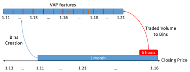
Figure 1. Illustration of VAP feature generation.

Trade direction and aggressiveness features. Finally, we enrich the feature space with information that is derived from the raw tick data and is intended to capture the aggressiveness of trading volume. We use a method from (Bouchaud et al., 2018) that classifies each trade (and its associated volume) as “aggressive” or “non-aggressive”. If a trade triggers a price change (in practice because, for example, the volume of an incoming market order is higher than the available volume at the best quote on the opposite side of the limit order book) then the trade and its volume is marked as aggressive; otherwise the trade and its volume is marked as non-aggressive. (Bouchaud et al., 2018) found this type of classification had predictive value.

Using the raw tick data, we used this method to classify all trades as aggressive or non-aggressive. We further classify trades and the corresponding volume as buyer or seller initiated in the spirit of the Lee-Ready indicator (Lee and Ready, 1991). In a limit order book market, such as the futures market in our investigation, a trade is triggered by an incoming order, which is matched against sitting order(s) that are already in the book. If this incoming order is a buy (sell), which is normally apparent from the data if one knows the best bid and ask when the order arrives, then we classify this trade as a buy (sell) trade and volume.

With these two categorizations of trades and their volume into buy/sell and aggressive/non-aggressive, we construct for a given 30-minute bar, the following features (all min-max normalized in the same way as the FS1 features): the total number of trades (the total volume is already included in FS1), the difference between buyer and seller initiated trade count, the difference between buyer and seller initiated volume, the non-aggressive volume, the non-aggressive trade count, the difference between buyer and seller initiated non-aggressive trade count, and the difference between buyer and seller initiated non-aggressive volume (given that we include total volume and trade count, we do not also include separate features for aggressive volume/trade count, since the totals and the non-aggressive features imply these). FS4 is formed from FS3 by augmenting it with these seven features.

4.1.4. Walk-forward cross-validation

Figure 2 illustrates the anchored walk-forward scheme that was used to create train, validation and test sets. The length of the initial train set used was 6 months; with the anchored scheme, the length of each subsequent train set gets longer. The length of all validation test sets used were 2 and 6 months respectively (a shorter validation set was used so as to keep as more data for training and testing).

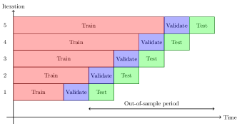
Figure 2. Walk-forward train-validation-test scheme.

4.1.5. Hyperparameter Tuning

As the design of the trading strategy will be based on the classifier’s predictions, one of our goals was to determine the best set of hyperparameters that will result to the most efficient ML classifiers. Popular methods that are used in the literature for hyperparameter tuning are the Grid Search, Random Search and Bayesian optimization process. In this study, the Grid Search method was used due to its simplicity. To make a fair comparison across all classifiers, 12 hyperparameter combinations were used to define the best hyperparameter set of each classifier.

In both classification problems, at each walk-forward period, the best hyperparameter set was selected based on the highest validation Matthews Correlation Coefficient (MCC) value.

We used MCC as our metric to define best models because it is a balanced measure that takes into account true/false positives and negatives and it can be used for both binary and ternary classification problems. Its advantages can be found in (Chicco and Jurman, 2020).

For logistic regression, we set the maximum number of iterations equal to $\{250,500\}$, the optimization algorithm to $\{liblinear,saga\}$, and the inverse of regularization strength to $\{0.01,0.001,0.0001\}$. For all the other hyperparameters, we used the default values from scikit-learn. For random forests (Breiman, 2001), we used $\{500,1000,2000\}$ many trees, splitting criteria in $\{gini,entropy\}$, and $sqrt(\#\text{features})$ and $log2(\#\text{features})$ for the number of features to consider when looking for the best split. For all other hyperparameters for random forests, default values in scikit-learn were used.

The feed-forward and LSTM networks consist from the same hyperparameter combinations as they share a lot of common aspects. It is well known that neural networks have too many hyperparameters to set. In this study, four different network architectures and three different learning rates were defined. An architecture is defined by (number of features, number of hidden units in the first layer, number of hidden units in the second layer (if applicable), number of units in the output layer depending on the classification labels). For both binary and ternary classification, the following architectures were used: $(\#\text{features},512,\{2,3\})$, $(\#\text{features},256,\{2,3\})$, $(\#\text{features},512,256,\{2,3\})$, $(\#\text{features},256,128,\{2,3\})$. Learning values of $\{0.01,0.001,0.0001\}$ were used.

The feed-forward networks consist of an input layer, one or more hidden layers and an output layer. Rectified linear units (Nair and Hinton, 2010) were used as activation functions for all layers except the output layer, where softmax activation was used. In hidden layers, $l_{2}$ weight regularization method was applied to prevent overfitting. Batch normalization (Ioffe and Szegedy, 2015) was used on each layer, where for each batch it standardizes the inputs to a layer and reduces the number of training epochs. Dropout (Srivastava et al., 2014) was also used as a further protection against overfitting. The Adam optimizer with a decay of $1e^{-6}$ was used when the learning rate was equal to $0.0001$; for the other learning rates, a decay of $1e^{-4}$ was used.

There are two different types of LSTM networks: stateless and stateful. Stateless LSTM networks initialise the hidden and cell states freshly for each batch. Stateful LSTM networks pass to the second batch the hidden and cell states from the first batch, and so on. In this study, we use the stateful LSTM networks as we want the long-term memory to remember the content of the previous batches. In the LSTM layers, the hyperbolic tangent function was used as activation function and the softmax activation function in the output layer. In the hidden layers the l2 weight regularization method was applied. Batch normalization and dropout were also used. The Adam optimizer was used in the same way as on feed-forward networks. In the LSTM networks sequences of 48 (one day’s) timesteps were used.

4.1.6. Selective Classification

To create the selective classifiers, the SGR (Algorithm 1) was applied on the predicted probabilities for each non-selective binary/ternary classifier. Coverage is defined as the percentage of samples that have not been rejected by the SGR algorithm (coverage for the non-selective classifiers is always 100%). For different desired risk levels, the SGR algorithm applies selected thresholds allowing a trade-off between accuracy and coverage. The selection of the best selective classifier threshold for both binary and ternary was chosen to be the one that gives the highest MCC value (across all 2 or 3 classes respectively). Finally, for the ternary classification problem, the multiplier that determines which price moves get label 0, is selected based on the highest MCC value of just the buy and sell labels, a choice driven by our goal of having accurate buy/sell predictions as a basis for trading strategies.

4.2. Classification results

Ultimately, we use the (selective and non-selective) classifiers that we train as the basis for trading strategies. Before we do that, in this section we first analyze the trained classifiers, both selective and non-selective, purely on the classification task. We explore the relative performance of selective versus non-selective classification, binary versus ternary classification, the different classification algorithms and the different feature sets.

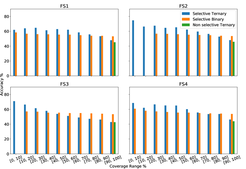
Figure 3. Accuracy/coverage trade-off of selective binary/ternary LSTM classifiers.

The first takeaway is that selective classification works as expected: By being selective and reducing coverage we are able to improve our accuracy on those data points where we do make a prediction. This can be seen in Tables 1 and 2, which show, for binary and ternary classifiers respectively, the chosen realized test coverage rates based on the chosen threshold levels. The resulting coverage levels show quite stringent selectivity, ranging between 37% and 63% for the binary classifiers, and between 17% and 55% for ternary classifiers. We see that in every single case (i.e., across all classification approaches and feature sets), the selectivity results in an improvement in accuracy. This shows the potential of selective classification; however to properly assess this potential in the context of designing trading strategies requires backtesting that we will return to in due course.

Figure 3 shows the coverage/accuracy trade-off for the selective classifiers, with results for the ternary non-selective classifier given as a reference point. Here we see that, broadly speaking, the accuracy coverage trade-off of the selective classifiers (binary and ternary) are in line with the results of (Geifman and El-Yaniv, 2017), where for lower coverage values we have higher accuracy levels.

Table 1. Binary classifiers: Non-selective, selective accuracy and coverage rates on the test set.

Models	Features	Non-sel. Accuracy %	Selective Accuracy %	Coverage %
LR	FS1	$53.24$	$54.64$	$63.17$
	FS2	$53.50$	$55.79$	$47.53$
	FS3	$53.46$	$55.43$	$51.32$
	FS4	$53.47$	$55.85$	$47.45$
RF	FS1	$51.23$	$52.19$	$61.14$
	FS2	$52.13$	$53.95$	$56.62$
	FS3	$52.38$	$54.20$	$48.68$
	FS4	$52.45$	$54.29$	$41.86$
NN	FS1	$52.67$	$55.24$	$37.03$
	FS2	$53.16$	$55.37$	$44.53$
	FS3	$52.50$	$54.32$	$44.43$
	FS4	$52.55$	$54.20$	$49.06$
LSTM	FS1	$53.05$	$54.95$	$57.13$
	FS2	$53.47$	$55.84$	$47.77$
	FS3	$53.28$	$55.74$	$37.34$
	FS4	$53.66$	$56.52$	$38.14$

The tables also show the relative performance of the different classification methods, and of the different feature sets. Ultimately, the results are mixed, but clear cut observations we can make include the following. Logistic regression (LR) performed well both for the binary and ternary setups. Random forests (RF) struggled with the richer feature sets, very possibly due to overfitting. LSTMs performed well for both binary and ternary setups, but were clearly beaten by logistic regression in the ternary setup. In terms of the feature sets while the results are mixed, it is certainly fair to say that there is no clear evidence of a benefit to using the richer feature sets, with FS2 arguably being the best choice on balance.

Table 2. Ternary classifiers: Non-selective, selective accuracy and coverage rates on the test set, with the highest in-sample MCC of the buy and sell labels used to choose the multiplier.

Models	Features	Non-sel. Accuracy %	Selective Accuracy %	Coverage %
LR	FS1	$44.48$	$58.61$	$19.80$
	FS2	$46.12$	$63.00$	$17.95$
	FS3	$43.83$	$59.67$	$16.83$
	FS4	$46.25$	$63.00$	$22.34$
RF	FS1	$54.66$	$57.63$	$55.11$
	FS2	$44.08$	$49.78$	$31.25$
	FS3	$42.71$	$49.35$	$24.69$
	FS4	$42.90$	$48.71$	$32.41$
NN	FS1	$43.16$	$52.25$	$30.69$
	FS2	$44.70$	$55.85$	$25.17$
	FS3	$43.84$	$49.41$	$54.48$
	FS4	$47.27$	$55.97$	$47.46$
LSTM	FS1	$45.29$	$56.13$	$33.88$
	FS2	$45.90$	$59.07$	$31.89$
	FS3	$42.67$	$55.86$	$25.61$
	FS4	$43.92$	$54.84$	$24.71$

Given that our selective classifiers abstain on a significant proportion of samples, it is natural to explore how the abstentions are distributed through time. For example, do we abstain for very long periods of time? We investigate this, and, as shown in Figure 4, find that this is not the case, namely, that the gaps between predictions are generally not that large. Across all classification methods and for all features sets, the distribution of gaps between predictions appears to follow a power law distribution, and the majority of gaps are between $30$-minutes (the smallest possible) and $2.5$ hours. This is certainly not a requirement for a good classifier (and resulting trading strategy), but is reassuring in so far as it shows that suitable conditions for making predictions do occur regularly.

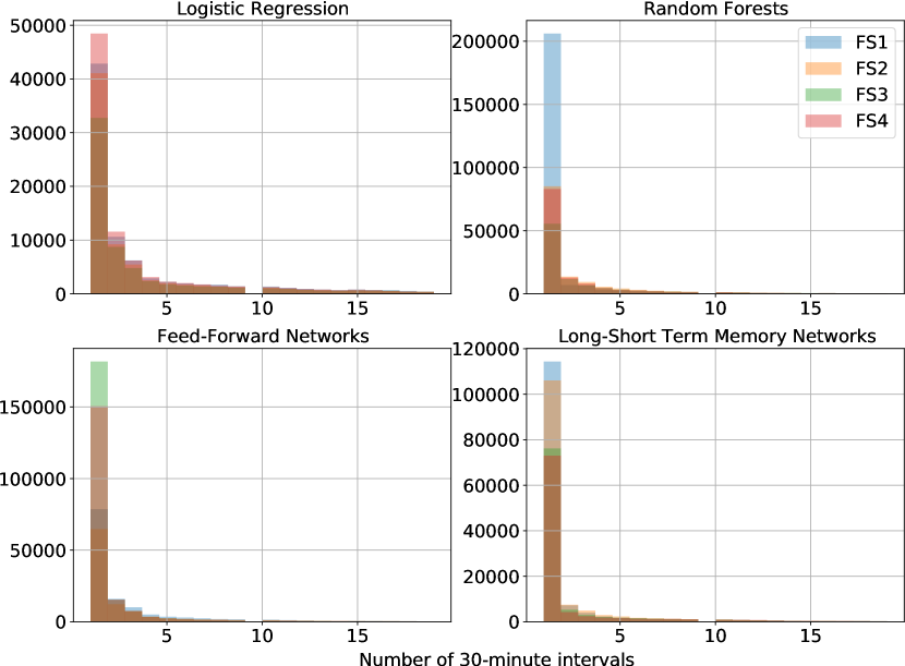
Figure 4. Time distribution of the non-abstained samples.

Binary versus ternary classification. To finish this section, we discuss the performance of binary versus ternary classification. Tables 1 and 2 show significant differences between the binary and ternary cases in terms of both coverage and accuracy. One consistent pattern is that total non-selective accuracy is lower in the ternary case. This is not a surprise since the ternary classifier has to be strictly more discerning to achieve the same level of total accuracy as the binary classifier. A clear but not totally consistent pattern is that the total selective accuracy is higher in the ternary case, and the coverage is less in the ternary case. A possible explanation is that a selective ternary classifier is optimized based on both the coverage threshold and the multiplier that determines the labelling. The multiplier is chosen to optimize the MCC of the buy and sell labels. In the ternary selective case we find that, in general, it picks relatively high multiplier values which gives a relatively large number of 0 labels – this can be seen in Table 3, which shows the resulting distribution of labels in the test set (with only FS1 for brevity), where between 45 and 54% of the labels are 0 (flat), significantly higher than $\frac{1}{3}$. The coverage threshold is set to optimize the MCC across all (2 or 3) classes, and in the ternary case this optimization step when combined with the extra multiplier parameter, is giving better selective accuracy via lower coverage (higher coverage thresholds). Table 3 also shows differences between models in terms of the distribution of true labels among all samples and just those where the model abstains; for example, unlike the other models, the RF (random forests) model has a very large difference, 54% versus 36%, in the percentage of flat labels. This arises due to the RF model being very certain of its flat predictions, so abstaining relatively less for this label.

Table 3. True labels percentages across all test data, for all rows (“All”) and just abstained rows (“Abs.”) for the ternary selective classifiers with FS1. All true labels percentages are rounded.

Label	Rows	LR	RF	NN	LSTM
short	All	$26$	$23$	$28$	$27$
	Abs.	$27$	$32$	$30$	$29$
flat	All	$49$	$54$	$45$	$47$
	Abs.	$46$	$36$	$41$	$42$
long	All	$26$	$23$	$28$	$27$
	Abs.	$27$	$32$	$29$	$29$

Given our intended trading application, whether binary or ternary classification is better cannot easily be determined by (selective) accuracy, not least because correct and incorrect classifications can correspond to very different profit and loss amounts for a trading strategy. In the next section, we backtest the resulting trading strategies to explore this further.

5. Trading strategies

As we just noted, from a trading perspective some misclassifications are more costly than others. We next turn our classifiers into trading strategies which we backtest and compare.

5.1. Backtesting methodology

We will hold a position that is consistent with our predictions. That is, whenever we make a prediction of label -1, we will hold a short position, and when we predict label 1 we will take a long position. Position sizing is discussed below, along with slippage which will be applied whenever we trade (which is determined by the desired position sign, namely long/short/flat).

Thus, the behaviour of our binary/ternary selective/non-selective classifiers will be as follows:

• A non-selective binary classifier is thus “always in the market” (never flat).

• A selective binary classifier stays flat (i.e., does not take a position) precisely when the classifier abstains.

• A non-selective ternary classifier stays flat when the predicted label is 0.

• A selective ternary classifier stays flat either when the predicted label is 0, or when the classifier abstains.

We trade when the desired position sign changes. The position size for a given commodity (specified as a number of futures contracts) is set to be inversely proportional to a 5-day moving average of the absolute close-on-close move in dollar terms. This simple scheme is used so that we can reasonably aggregate profit and loss across the commodities. To be conservative, slippage was paid on every contract traded. The amount of slippage was defined as a multiple $\{0,0.1,\dots,0.5\}$ of the tick size for the respective commodity. The number of contracts traded are determined by the difference between the current position and desired position, so, for example, if the current position is 6 contracts (long) and the desired position is 2 contracts (short), then the resulting trade would sell 8 contracts (paying slippage on each).

The backtest applies the classifiers to each commodity independently and trades accordingly, aggregating the resulting profit and loss across the commodities. In order to get a risk-adjusted measure, we compute and report a profit-based variant of the Sharpe Ratio (i.e., one that assumes a constant underlying cost to each trade, which we consider fine as we only use the resulting numbers for roughly assessing relative performance).

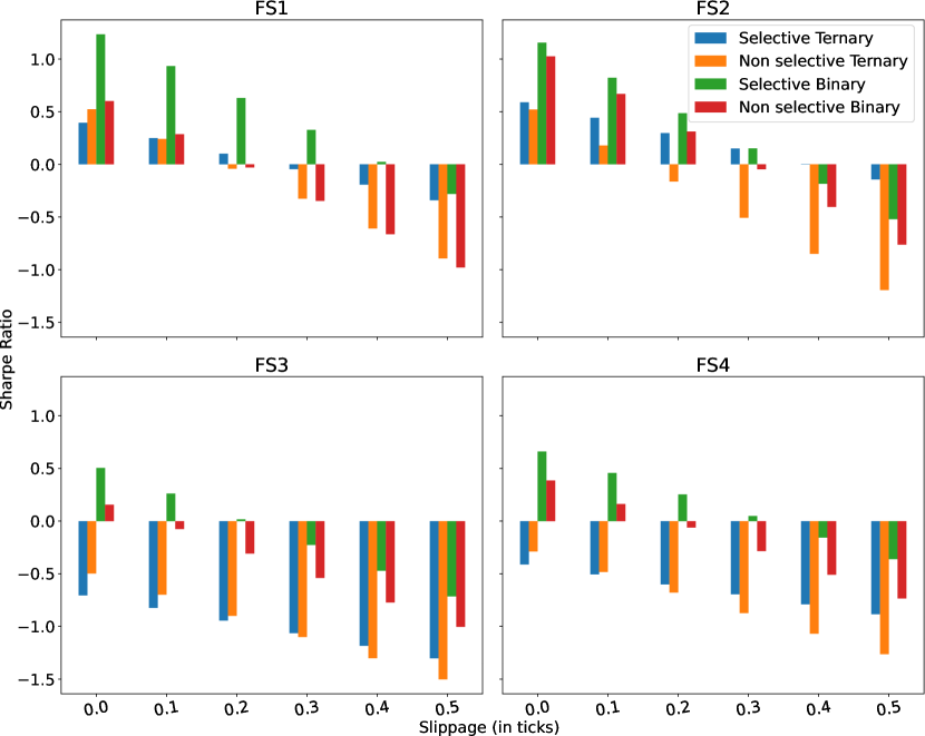
Figure 5. Sharpe Ratios for backtested ternary/ binary selective and non-selective Feed-Forward network classifiers.

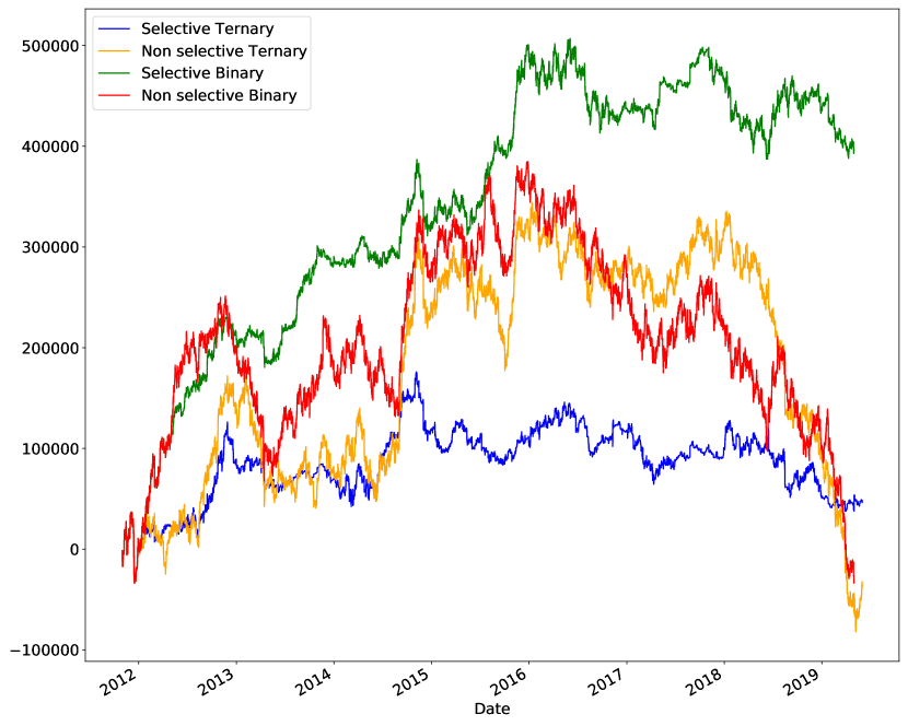
Figure 6. Indicative equity curves corresponding to Figure 5, feature set FS1 and slippage level $0.2$.

5.2. Backtesting results

All reported backtesting results are out-of-sample (see Figure 2).

In Figure 5, the results of the feed-forward networks backtesting process are presented. Figure 6 shows the equity curves that correspond to the FS1 and slippage level 0.2 results within Figure 5. As slippage increases, both binary and ternary selective classifiers have better Sharpe Ratio values compared to their respective non-selective classifiers. From the four features sets, the FS2 feature set has the best Sharpe Ratio results, taking into account the results of each classifier for all slippage values. The FS3 feature set has the worst Sharpe Ratio values compared to the other features sets. In particular, since FS1 tended to provide better results than FS4, we did not see the benefits of our richest feature sets.

In Table 4, the Sharpe Ratio results of all the classifiers and features sets are presented for slippage set to $0.3$ ticks. At this level of slippage, many configurations are not profitable, but some are, including: With all four feature sets, the logistic regression (LR) binary selective classifiers were profitable, as are some other configurations of this type of classifier; for FS1 and FS2, the feed-forward network (NN) binary selective classifiers were profitable; for FS1 and FS2, the random forests (RF) ternary selective classifiers were profitable. The classifiers using LSTMs are never profitable, which may well just reflect the difficulty in training these types of models.

Table 4. Sharpe Ratios for the binary/ternary selective and non-selective classifiers with slippage at $0.3$ ticks.

Models	Features	Selective Binary	Non-sel. Binary	Selective Ternary	Non-sel. Ternary
LR	FS1	$0.02$	$0.16$	$-0.12$	$-0.60$
	FS2	$0.21$	$0.02$	$0.03$	$-0.97$
	FS3	$0.15$	$-0.08$	$-0.16$	$-0.82$
	FS4	$0.28$	$-0.03$	$-0.20$	$-0.31$
RF	FS1	$-1.61$	$-1.60$	$-0.35$	$-1.46$
	FS2	$-0.57$	$-0.61$	$-0.24$	$-1.04$
	FS3	$-0.03$	$-0.61$	$0.57$	$-1.03$
	FS4	$-0.41$	$-0.75$	$0.35$	$-0.10$
NN	FS1	$0.33$	$-0.35$	$-0.05$	$-0.33$
	FS2	$0.15$	$-0.05$	$0.15$	$-0.51$
	FS3	$-0.23$	$-0.54$	$-1.06$	$-1.10$
	FS4	$0.05$	$-0.29$	$-0.70$	$-0.87$
LSTM	FS1	$-0.86$	$-0.89$	$-0.23$	$-0.76$
	FS2	$-0.81$	$-0.67$	$-0.29$	$-1.23$
	FS3	$-0.70$	$-0.87$	$-0.40$	$-1.22$
	FS4	$-0.43$	$-0.69$	$-0.12$	$-1.10$

We consider these results to be a promising proof of concept for this trading approach, especially given that many parameters of the method were not optimized and just set as intuitively reasonable choices. This also applies to the feature sets; there is a lot of scope to improve these and other aspects of the setup.

6. Conclusions/ Future Work

This study presents an application of selective classification in futures time series, and backtests trading strategies based on the classifier’s predictions. We found that:

• The selective classifiers performed better than their non-selective counterparts in terms of accuracy.

• Lower coverage values resulted in higher accuracy levels.

• The selective classifiers had better backtesting results compared to their respective non-selective classifiers.

• The results did not demonstrate any advantage of the richer feature sets.

• Selective classification reduced the misclassification percentages by abstention, which helped the trading strategies to avoid losses.

• The selective binary classifiers had better backtesting results compared to the selective and non-selective ternary classifiers.

The results show the potential of selective classification, as the selective classifiers performed better than their non-selective counterparts in terms of accuracy and backtesting results. It would be interesting to explore the use of other selective classification algorithms, such as (Geifman and El-Yaniv, 2019; Thulasidasan et al., 2019). As discussed at the end of Section 4.2, the ternary classifiers worked quite differently from the binary classifiers and appeared promising when looking only at accuracy, but in the end provided worse backtesting results. It would be interesting to explore hyperparameter optimization based on backtesting results directly, rather than the MCC criterion.

- (1)
- Bao et al. (2017) Wei Bao, Jun Yue, and Yulei Rao. 2017. A deep learning framework for financial time series using stacked autoencoders and long-short term memory. PloS one 12, 7 (2017).
- Bartlett and Wegkamp (2008) Peter L. Bartlett and Marten H. Wegkamp. 2008. Classification with a Reject Option using a Hinge Loss. J. Mach. Learn. Res. 9 (2008), 1823–1840.
- Borovkova and Tsiamas (2019) Svetlana Borovkova and Ioannis Tsiamas. 2019. An ensemble of LSTM neural networks for high-frequency stock market classification. Journal of Forecasting 38, 6 (2019), 600–619.
- Bouchaud et al. (2018) Jean-Philippe Bouchaud, Julius Bonart, Jonathan Donier, and Martin Gould. 2018. Trades, quotes and prices: financial markets under the microscope. Cambridge University Press.
- Box and Cox (1964) George EP Box and David R Cox. 1964. An analysis of transformations. Journal of the Royal Statistical Society: Series B (Methodological) 26, 2 (1964), 211–243.
- Breiman (2001) Leo Breiman. 2001. Random forests. Machine learning 45, 1 (2001), 5–32.
- Chicco and Jurman (2020) Davide Chicco and Giuseppe Jurman. 2020. The advantages of the Matthews correlation coefficient (MCC) over F1 score and accuracy in binary classification evaluation. BMC genomics 21, 1 (2020), 6.
- Chow (1970) C. K. Chow. 1970. On optimum recognition error and reject tradeoff. IEEE Trans. Information Theory 16, 1 (1970), 41–46.
- Cortes et al. (2016) Corinna Cortes, Giulia DeSalvo, and Mehryar Mohri. 2016. Boosting with Abstention. In Proc. of NIPS. 1660–1668.
- El-Yaniv and Wiener (2010) Ran El-Yaniv and Yair Wiener. 2010. On the Foundations of Noise-free Selective Classification. J. Mach. Learn. Res. 11 (2010), 1605–1641.
- Geifman and El-Yaniv (2017) Yonatan Geifman and Ran El-Yaniv. 2017. Selective Classification for Deep Neural Networks. In Proc. of NIPS.
- Geifman and El-Yaniv (2019) Yonatan Geifman and Ran El-Yaniv. 2019. SelectiveNet: A Deep Neural Network with an Integrated Reject Option. In Proc. of ICML.
- Gu et al. (2020) Shihao Gu, Bryan Kelly, and Dacheng Xiu. 2020. Empirical Asset Pricing via Machine Learning. The Review of Financial Studies 33 (2020), 2223–2273.
- Hellman (1970) Martin E. Hellman. 1970. The Nearest Neighbor Classification Rule with a Reject Option. IEEE Trans. Systems Science and Cybernetics 6, 3 (1970), 179–185.
- Hochreiter and Schmidhuber (1997) Sepp Hochreiter and Jürgen Schmidhuber. 1997. Long short-term memory. Neural computation 9, 8 (1997), 1735–1780.
- Ioffe and Szegedy (2015) Sergey Ioffe and Christian Szegedy. 2015. Batch normalization: Accelerating deep network training by reducing internal covariate shift. arXiv preprint arXiv:1502.03167 (2015).
- Kim and Kim (2019) Taewook Kim and Ha Young Kim. 2019. Forecasting stock prices with a feature fusion LSTM-CNN model using different representations of the same data. PloS one 14, 2 (2019).
- Lee and Ready (1991) Charles MC Lee and Mark J Ready. 1991. Inferring trade direction from intraday data. The Journal of Finance 46, 2 (1991), 733–746.
- Nair and Hinton (2010) Vinod Nair and Geoffrey E Hinton. 2010. Rectified linear units improve restricted boltzmann machines. In Proc. of ICML.
- Patel et al. (2015) Jigar Patel, Sahil Shah, Priyank Thakkar, and Ketan Kotecha. 2015. Predicting stock and stock price index movement using trend deterministic data preparation and machine learning techniques. Expert systems with applications 42, 1 (2015), 259–268.
- Sezer et al. (2020) Omer Berat Sezer, Mehmet Ugur Gudelek, and Ahmet Murat Ozbayoglu. 2020. Financial time series forecasting with deep learning: A systematic literature review: 2005–2019. Applied Soft Computing 90 (2020), 106181.
- Srivastava et al. (2014) Nitish Srivastava, Geoffrey Hinton, Alex Krizhevsky, Ilya Sutskever, and Ruslan Salakhutdinov. 2014. Dropout: a simple way to prevent neural networks from overfitting. The Journal of Machine Learning Research 15, 1 (2014), 1929–1958.
- Steidlmayer and Hawkins (2003) J Peter Steidlmayer and Steven B Hawkins. 2003. Steidlmayer on Markets: Trading with Market Profile. Vol. 173. John Wiley & Sons.
- Thulasidasan et al. (2019) Sunil Thulasidasan, Tanmoy Bhattacharya, Jeff A. Bilmes, Gopinath Chennupati, and Jamal Mohd-Yusof. 2019. Combating Label Noise in Deep Learning using Abstention. In Proc. of ICML.
- Wiener and El-Yaniv (2015) Yair Wiener and Ran El-Yaniv. 2015. Agnostic Pointwise-Competitive Selective Classification. J. Artif. Intell. Res. 52 (2015), 171–201. https://doi.org/10.1613/jair.4439