Compact extended formulations for low-rank functions with indicator variables

Abstract.

We study the mixed-integer epigraph of a special class of convex functions with non-convex indicator constraints, which are often used to impose logical constraints on the support of the solutions. The class of functions we consider are defined as compositions of low-dimensional nonlinear functions with affine functions Extended formulations describing the convex hull of such sets can easily be constructed via disjunctive programming, although a direct application of this method often yields prohibitively large formulations, whose size is exponential in the number of variables. In this paper, we propose a new disjunctive representation of the sets under study, which leads to compact formulations with size exponential in the dimension of the nonlinear function, but polynomial in the number of variables. Moreover, we show how to project out the additional variables for the case of dimension one, recovering or generalizing known results for the convex hulls of such sets (in the original space of variables). Our computational results indicate that the proposed approach can significantly improve the performance of solvers in structured problems.

Keywords. Mixed-integer nonlinear optimization, convexification, disjunctive programming, indicator variables.

1. Introduction

In this paper, we consider a general mixed-integer convex optimization problem with indicator variables

$$\min_{x,z}\;\left\{F(x):(x,z)\in\mathcal{F}\subseteq\mathbb{R}^{n}\times\{0,1\}^{n},x_{i}(1-z_{i})=0\;\forall i\in[n]\right\},$$ (1)

where $F:\mathbb{R}^{n}\to\mathbb{R}$ is a convex function, $\mathcal{F}$ is the feasible region, and $[n]\stackrel{{\scriptstyle\mathclap{\text{\tiny def}}}}{{=}}\{1,2,\dots,n\}$. Each binary variable $z_{i}$ indicates whether a given continuous variable $x_{i}$ is zero or not. In other words, $z_{i}=0\implies x_{i}=0$, and $z_{i}=1$ allows $x_{i}$ to take any value. Optimization problem (1) arises in a variety of settings, including best subset selection problems in statistics [16], and portfolio optimization problems in finance [17]. In practice, the objective function often has the form $F(x)=\sum_{i\in[m]}f_{i}(x)$, where each $f_{i}(x)$ is a composition of a relatively simple convex function and a low-rank linear map. In the context of machine learning and statistics, $m$ represents the number of samples, and in turn, each index $i$ corresponds to one observed data point. Besides linear regression for which each $f_{i}$ is a rank-one quadratic function, another prominent class of statistical models is logistic regression –widely used for classification problems–, where each $f_{i}$ is a composition of a logistic function and a linear function, that is, $f_{i}(x)=\ln\left(e^{a_{i}^{\top}x}+1\right)$ for a suitable vector $a_{i}\in\mathbb{R}^{n}$. Moreover, in some scenarios [46], decision variables are additionally required to be nonnegative for better interpretability and possess certain combinatorial structures such as sparsity. Such optimization problems can be readily modeled as (1) [47]. The above observation motivates the need for a comprehensive study of the mixed-integer set

$$\mathcal{Q}\stackrel{{\scriptstyle\mathclap{\text{\tiny def}}}}{{=}}\left\{(t,x,z)\in\mathbb{R}^{n+1}\times\{0,1\}^{n}:\;\begin{aligned} &t\geq f(x),x_{i}\geq 0\;\forall i\in\mathcal{I}_{+},\\ &z\in\{0,1\}^{n},x_{i}(1-z_{i})=0\;\forall i\in[n]\end{aligned}\right\},$$ (2)

where $f(x)=g(Ax)+{c}^{\top}{x}$, $g:\mathbb{R}^{k}\to\mathbb{R}$ is a proper closed convex function, $A$ is a $k\times n$ matrix, $c\in\mathbb{R}^{n}$, and $\mathcal{I}_{+}\subseteq[n]$ is the subset of variables restricted to be non-negative.

Disjunctive programming is a powerful modeling tool to represent a nonconvex optimization problem in the form of disjunctions, especially when binary variables are introduced to encode the logical conditions such as sudden changes, either/or decisions, implications, etc. [12]. The theory of linear disjunctive programming was first pioneered by Egon Balas in 1970s [11, 9, 10, 13], and later extended to the nonlinear case [19, 48, 42, 30, 14, 18, 40, 41, 43, 20, 52]. Once a mixed-integer set is modeled as a collection of disjunctive sets, its convex hull can be described easily as a Minkowski sum of the scaled convex sets with each obtained by creating a copy of original variables. Such extended formulations are the strongest possible convex relaxations of the mixed-integer set under study. However, a potential downside of such formulations is that, often, the number of additional variables required in the description of the convex hull is exponential in the number of binary variables. Thus, a direct application of disjunctive programming as mentioned can be unfavorable in practice.

A possible approach to implement the extended formulation induced by disjunctive programming in an efficient way is to reduce the number of additional variables introduced in the model without diminishing the relaxation strength. In principle, this goal can be achieved by means of Fourier-Motzkin elimination [22]. This method is practical if the set under study can be naturally expressed using few disjunctions, e.g., to describe piecewise linear functions [2, 33], involves few binary variables [4, 27], or is separable [32]. However, projecting out variables can be very challenging even if $n=2$ [3, 23], not to mention in a high-dimensional setting. Regarding the nonlinear set with indicator variables $\mathcal{Q}$, in the simplest case where the MINLP is separable, it is known that the convex hull can be described by the perspective function of the objective function supplemented by the constraints defining the feasible region [1, 24, 25, 26, 32, 37, 50, 15].

Two papers [49] and [7] are closely related to our work. The mixed-integer sets studied in both can be viewed as a special realization of $\mathcal{Q}$ in (2). Wei et al., [49] characterize the closure of the convex hull if $\mathcal{Q}$ when the defining function $g$ is a univariate function and the continuous variables are free, i.e. $\mathcal{I}_{+}=\emptyset$. Atamtürk and Gómez, [7] study the setting with sign-constrained continuous variables, and univariate quadratic functions $g$: in such cases, the sign-restrictions resulted in more involved structures for the closure of the convex hull of $\mathcal{Q}$.

Contributions and outline

In this paper we show how to construct extended formulations of set $\mathcal{Q}$, requiring at most $\mathcal{O}(n^{k})$ copies of the variables. In particular, if the dimension $k$ is small, then the resulting formulations are indeed much smaller than those resulting from a natural application of disjunctive programming. Moreover, for the special case of $k=1$, we show how we are able to recover and improve existing results in the literature, either by providing smaller extended formulations (linear in $n$), or by providing convexifications in the original space of variables for a more general class of functions (arbitrarily convex and not necessarily differentiable). When applied to a class of sparse signal denoising and outlier detection problems, the new formulations proposed in this paper significantly outperforms the natural one whose relaxation yields a trivial lower bound of $0$. It also turns out that as $k$ increases, the resulting formulation becomes even more powerful.

The rest of the paper is organized as follows. In Section 2, we provide relevant background and the main result of the paper: a compact extended formulation of $\mathcal{Q}$. In Section 3, using the results in Section 2, we derive the explicit form of the convex hull $\mathcal{Q}$ for $k=1$ in the original space of variables. In Section 4, we present the complexity results showing that tractable convexifications of $\mathcal{Q}$ are unlikely if additional constraints are imposed on the continuous variables. In Section 5, we present the numerical experiments. Finally, in Section 6, we conclude the paper.

2. A convex analysis perspective on convexification

In this section, we first introduce necessary preliminaries in convex analysis and notations adopted in this paper. After that we present our main results and their connections with previous works in literature.

2.1. Notations and preliminaries

Throughout this paper, we assume $f(x)$ is a proper closed convex function from $\mathbb{R}^{n}$ to $\mathbb{R}\cup\{+\infty\}$. If $f(x)<+\infty$ for all $x$, $f(x)$ is called finite. We denote the effective domain of $f$ by $\operatorname*{dom}(f)$ and the convex conjugate of $f(\cdot)$ by $f^{*}(\cdot)$ which is defined as

$$f^{*}(\alpha)\stackrel{{\scriptstyle\mathclap{\text{\tiny def}}}}{{=}}\max_{x}\;{\alpha}^{\top}{x}-f(x).$$

The perspective function of $f(\cdot)$ is defined as

$$f^{\pi}(x,\lambda)\stackrel{{\scriptstyle\mathclap{\text{\tiny def}}}}{{=}}\begin{cases}\lambda f\left(\frac{x}{\lambda}\right)&\text{if }\lambda\geq 0\\ +\infty&\text{o.w.},\end{cases}$$

where $0f(x/0)$ is interpreted as the recession function of $f$ at $x$. By this definition, the function $f^{\pi}(\cdot)$ is homogeneous, closed and convex; see Section 8 in [44]. Moreover, we borrow the term rank which is normally defined for an affine mapping and extend its definition to a general nonlinear convex function.

Definition 1 (Rank of convex functions).

Given a proper closed convex function $f(x)$, the rank of $f$, denoted $\operatorname{rank}(f)$, is defined as the smallest integer $k$ such that $f(x)$ can be expressed in the form $f(x)=g(Ax)+{c}^{\top}{x}$ for some closed convex function $g(\cdot)$, a $k\times n$ matrix $A$ and a vector $c\in\mathbb{R}^{n}$.

For example, the rank of an affine function $f(x)={c}^{\top}{x}$ is simply $0$. The rank of a convex quadratic function $f(x)=x^{\top}A{x}$ coincides with $\operatorname{rank}(A)$, where $A\succeq 0$ is a positive semidefinite (PSD) matrix.

We let $\mathbf{e}$ be the vector of all ones (whose dimension can be inferred from the context). For any vector $y\in\mathbb{R}^{n}$ and index set $\mathcal{J}\subseteq[n]$, we denote $y(\mathcal{J})=\sum_{j\in\mathcal{J}}y_{j}$. For a set $\mathcal{S}$, we denote the convex hull of $S$ as $\text{conv}(\mathcal{S})$, and its closure as $\text{cl conv}(\mathcal{S})$. For any scalar ${\lambda}\geq 0$ and two generic sets $\mathcal{S}_{1}$, $\mathcal{S}_{2}$ in a proper Euclidean space, we define $\lambda\mathcal{S}_{1}\stackrel{{\scriptstyle\mathclap{\text{\tiny def}}}}{{=}}\{\lambda x:x\in\mathcal{S}_{1}\}$ and $\mathcal{S}_{1}+\mathcal{S}_{2}\stackrel{{\scriptstyle\mathclap{\text{\tiny def}}}}{{=}}\{x^{1}+x^{2}:x^{1}\in\mathcal{S}_{1},x^{2}\in\mathcal{S}_{2}\}$ is the Minkowski sum. We denote the indicator function of $\mathcal{S}$ by $\delta(x;\mathcal{S})$, which is defined as $\delta(x;\mathcal{S})=0$ if $x\in\mathcal{S}$ and $\delta(x;\mathcal{S})=+\infty$ otherwise. By the above notations, the convex conjugate of $\delta(x;\mathcal{S})$ is

$$\delta^{*}(\alpha;\mathcal{S})=\max_{x}\;{\alpha}^{\top}{x}-\delta(x;\mathcal{S})=\max_{x\in\mathcal{S}}\;{\alpha}^{\top}{x},$$

which is known as the support function of $\mathcal{S}$. To be consistent with the definition of $0f(x/0)$, we interpret $0\mathcal{S}$ as the recession cone of $\mathcal{S}$ throughout this paper. The derivation of the succeeding work relies on the following one-to-one correspondence between closed convex sets and support functions, whose proof can be found in classical books of convex analysis, e.g. Section 13 in [44] and Chapter C.2 in [38].

Proposition 1.

Given a set $\mathcal{S}$ and a closed convex set $\mathcal{T}$, $\mathcal{T}=\text{cl conv}(\mathcal{S})$ if and only if $\delta^{*}(\cdot;\mathcal{T})=\delta^{*}(\cdot;\mathcal{S})$.

For convenience, we repeat the set of interest:

$$\mathcal{Q}\stackrel{{\scriptstyle\mathclap{\text{\tiny def}}}}{{=}}\left\{(t,x,z)\in\mathbb{R}^{n+1}\times\{0,1\}^{n}:\quad\begin{aligned} &t\geq f(x),x_{i}\geq 0\;\forall i\in\mathcal{I}_{+},\\ &x_{i}(1-z_{i})=0\;\forall i\in[n]\end{aligned}\right\},$$

where $f(x)=g(Ax)+{c}^{\top}{x}$ is a proper closed convex function.

Note that if the complementary constraints $x_{i}(1-z_{i})=0$ are removed from $\mathcal{Q}$, then $x$ and $z$ are decoupled and $\text{cl conv}(\mathcal{Q})$ reduces simply to $\mathcal{X}\times[0,1]^{n}$, where

$$\mathcal{X}\stackrel{{\scriptstyle\mathclap{\text{\tiny def}}}}{{=}}\left\{(t,x)\in\mathbb{R}^{n+1}:t\geq f(x),x_{i}\geq 0\;\forall i\in\mathcal{I}_{+}\right\}.$$

For the purpose of decomposing $\text{cl conv}(\mathcal{Q})$, for any $\mathcal{I}\subseteq[n]$, define the following sets:

$$\mathcal{X}(\mathcal{I})\stackrel{{\scriptstyle\mathclap{\text{\tiny def}}}}{{=}}\mathcal{X}\cap\{(t,x):x_{i}=0\;\forall i\notin\mathcal{I}\},$$ (3)

$$\mathcal{Z}(\mathcal{I})\stackrel{{\scriptstyle\mathclap{\text{\tiny def}}}}{{=}}\left\{z\in\{0,1\}^{n}:z_{i}=1\;\forall i\in\mathcal{I}\right\},$$

$$\mathcal{V}(\mathcal{I})\stackrel{{\scriptstyle\mathclap{\text{\tiny def}}}}{{=}}\mathcal{X}(\mathcal{I})\times\mathcal{Z}(\mathcal{I}).$$

Notice that for any $(t,x,z)\in\mathcal{V}(\mathcal{I})$, either $x_{i}=0$ or $z_{i}=1\;\forall i\in[n]$. Therefore, $x_{i}(1-z_{i})=0\;\forall i\in[n]$ and thus $\mathcal{V}(\mathcal{I})\subseteq\mathcal{Q}$. Furthermore, $\mathcal{Q}$ can be expressed as a disjunction

$$\mathcal{Q}=\bigcup_{\mathcal{I}\subseteq[n]}\mathcal{V}(\mathcal{I}).$$ (4)

Standard disjunctive programming techniques for convexification of $\mathcal{Q}$ are based on (4), creating copies of variables for every $I\subseteq[n]$, resulting in an exponential number of variables.

Finally, define

$$\mathcal{R}\stackrel{{\scriptstyle\mathclap{\text{\tiny def}}}}{{=}}\{(t,x,z):t\geq 0,\;Ax=0,x_{i}\geq 0,\;\forall i\in\mathcal{I}_{+},\;z_{i}=1,\;\forall i\in[n]\},$$ (5)

which is a closed convex set. For any $y\in\mathbb{R}^{n}$, we denote the support of $y$ by $\operatorname{supp}(y)\stackrel{{\scriptstyle\mathclap{\text{\tiny def}}}}{{=}}\{i:y_{i}\neq 0\}$

2.2. Convex hull characterization

In this section, we aim to characterize $\text{cl conv}(\mathcal{Q})$. We first show that if $f(x)$ is homogeneous, under mild conditions, $\text{cl conv}(\mathcal{Q})$ is simply the natural relaxation of $\mathcal{Q}$.

Proposition 2.

If $f(x)$ is a homogeneous function, then $\text{cl conv}(\mathcal{Q})=\mathcal{X}\times[0,1]^{n}$.

Proof.

Since $f$ is homogeneous, each set $\mathcal{X}(\mathcal{I})$ is a closed convex cone. Moreover, $\mathcal{I}_{1}\subseteq\mathcal{I}_{2}$ implies that $\mathcal{X}(\mathcal{I}_{1})\subseteq\mathcal{X}(\mathcal{I}_{2})$, which further implies that

$$\mathcal{X}(\mathcal{I}_{2})\subseteq\mathcal{X}(\mathcal{I}_{1})+\mathcal{X}(\mathcal{I}_{2})\subseteq\mathcal{X}(\mathcal{I}_{2})+\mathcal{X}(\mathcal{I}_{2})=\mathcal{X}(\mathcal{I}_{2}),$$ (6)

where the last equality results from that $\mathcal{X}(\mathcal{I}_{2})$ is conic. Hence, equality holds throughout (6). By (4),

$$\text{cl conv}(\mathcal{Q})=\text{cl conv}\left(\bigcup_{\mathcal{I}\subseteq[n]}\mathcal{V}(\mathcal{I})\right)$$

$$= \text{cl conv}\left(\;\smashoperator[]{\bigcup_{\mathcal{I}\subseteq[n]}^{}}\mathcal{X}(\mathcal{I})\times\text{conv}(\mathcal{Z}(\mathcal{I}))\right) \mathcal{X}(\mathcal{I}) \mathcal{X},\mathcal{Z}$$ ( is convex; are decoupled)

$$= \bigcup_{\lambda\in\mathbb{R}_{+}^{2^{n}}:\mathbf{e}^{\top}\lambda=1}\;\sum_{\mathcal{I}\subseteq[n]}\lambda_{\mathcal{I}}\left(\mathcal{X}(\mathcal{I})\times\text{conv}(\mathcal{Z}(\mathcal{I}))\right)$$

$$= \bigcup_{\lambda\in\mathbb{R}_{+}^{2^{n}}:\mathbf{e}^{\top}\lambda=1}\;\mathcal{X}([n])\times\sum_{\mathcal{I}\subseteq[n]}\lambda_{\mathcal{I}}\text{conv}(\mathcal{Z}(\mathcal{I})) \mathcal{X}(\mathcal{I})$$ ( is conic and (6))

$$= \mathcal{X}\times\bigcup_{\lambda\in\mathbb{R}_{+}^{2^{n}}:\mathbf{e}^{\top}\lambda=1}\;\sum_{\mathcal{I}\subseteq[n]}\lambda_{\mathcal{I}}\text{conv}(\mathcal{Z}(\mathcal{I})) \mathcal{X} \mathcal{X}([n])$$ (=)

$$= \mathcal{X}\times[0,1]^{n}.$$

∎

Proposition 2 generalizes Proposition 1 of [29], from the fact that $f$ is the $\ell_{2}$ norm. Next, we present the main result of the paper, characterizing $\text{cl conv}(\mathcal{Q})$ without the assumption of homogeneity. In particular, we show that $\text{cl conv}(\mathcal{Q})$ can be constructed from substantially fewer disjunctions than those given in (4).

Theorem 1.

Assume $\operatorname{rank}(f)\leq k$ and $f(0)=0$. Then

$$\text{cl conv}(\mathcal{Q})=\text{cl conv}\left(\left(\bigcup_{\mathcal{I}:|\mathcal{I}|\leq k}\mathcal{V}({\mathcal{I}})\right)\cup\mathcal{R}\right){,}$$

where $\mathcal{V}(\mathcal{I})$ and $\mathcal{R}$ are defined in (3) and (5) respectively. Moreover, if $\left\{x\in\mathbb{R}^{n}:Ax=0,\;x_{i}\geq 0\;\forall i\in\mathcal{I}_{+}\right\}=\{0\}$, then $\mathcal{R}$ can be removed from the disjunction.

Informally, $\bigcup_{\mathcal{I}:|\mathcal{I}|\leq k}\mathcal{V}(I)$ and $\mathcal{R}$ correspond to the “extreme points” and “extreme rays” of $\text{cl conv}(\mathcal{Q})$, respectively. From (4), $\mathcal{Q}$ is a disjunction of exponentially many pieces of $\mathcal{V}(\mathcal{I})$. However, given a low-rank function $f$, Theorem 1 states that $\text{cl conv}(\mathcal{Q})$ can be generated (using disjunctive programming) from a much smaller number of sets $\mathcal{V}(\mathcal{I})$. We also remark that condition $f(0)=0$ plays a minor role in the derivation of Theorem 1. If $0\in\operatorname*{dom}(f)$ but $f(0)\neq 0$, one can study $f(x)-f(0)$.

Proof of Theorem 1.

Denote $\mathcal{S}=\smashoperator[]{\bigcup_{\mathcal{I}:|\mathcal{I}|\leq k}^{}}\mathcal{V}(I)\cup\mathcal{R}$. Since $\mathcal{V}(\mathcal{I})\subseteq\mathcal{Q}$ for all $\mathcal{I}$, and $\mathcal{R}\subseteq\mathcal{Q}$, we find that $\mathcal{S}\subseteq\mathcal{Q}$. Thus, $\delta^{*}(\cdot;\text{cl conv}(\mathcal{S}))=\delta^{*}(\cdot;\mathcal{S})\leq\delta^{*}(\cdot;\mathcal{Q}).$ Due to Proposition 1, it remains to prove the opposite direction, namely that $\delta^{*}(\cdot;\mathcal{S})\geq\delta^{*}(\cdot;\mathcal{Q})$.

Since $\operatorname{rank}(f)\leq k$, there exists $g(\cdot)$, $A\in\mathbb{R}^{k\times n}$ and $c$ such that $f(x)=g(Ax)+{c}^{\top}{x}$. Taking any $\alpha=(\alpha_{t},\alpha_{x},\alpha_{z})\in\mathbb{R}\times\mathbb{R}^{n}\times\mathbb{R}^{n}$, if $\alpha_{t}>0$, $\delta^{*}(\cdot;\mathcal{S})=\delta^{*}(\cdot;\mathcal{Q})=+\infty$ because $t$ is unbounded from above. We now assume $\alpha_{t}\leq 0$, and define

$$\ell(x,z)\stackrel{{\scriptstyle\mathclap{\text{\tiny def}}}}{{=}}\alpha_{t}g(Ax)+\left(\alpha_{x}+\alpha_{t}c\right)^{\top}{x}+\alpha_{z}^{\top}{z}.$$

Then $\delta^{*}(\alpha;\mathcal{S})=\max\{\ell(x,z):(t,x,z)\in\mathcal{S}\}$ and $\delta^{*}(\alpha;\mathcal{Q})=\max\{\ell(x,z):(t,x,z)\in\mathcal{Q}\}$. Given any fixed $(\bar{t},\bar{x},\bar{z})\in\mathcal{Q}$, consider the linear program

$$v^{*}\stackrel{{\scriptstyle\mathclap{\text{\tiny def}}}}{{=}}\max_{x\in\mathbb{R}^{n}} \left(\alpha_{x}+\alpha_{t}c\right)^{\top}{x}$$ (7)

s.t. $$Ax=A\bar{x}$$

$$\bar{x}_{i}x_{i}\geq 0 \forall i\in\operatorname{supp}(\bar{x})\subseteq\operatorname{supp}(\bar{z})$$

$$x_{i}=0 \forall i\in[n]\backslash\operatorname{supp}(\bar{x}).$$

Note that linear program (7) is always feasible setting $x=\bar{x}$. Moreover, every feasible solution (or direction) $x$ of (7) satisfies $x_{i}(1-\bar{z}_{i})=0$.

If $v^{*}=+\infty$, then there exists a feasible direction $d$ such that $Ad=0$ and $\left(\alpha_{x}+\alpha_{t}c\right)^{\top}{d}>0$. It implies that for any $r\geq 0$, $f(rd)=g(rAd)+rc^{\top}{d}=g(0)+r{c}^{\top}{d}=r{c}^{\top}{d}$. Hence, $(r{c}^{\top}{d},rd,\mathbf{e})\in\mathcal{R}\subseteq Q$. Furthermore,

$$\ell(rd,\mathbf{e})= \left(\alpha_{x}+\alpha_{t}c\right)^{\top}{d}r+{\alpha^{\top}_{z}}{\mathbf{e}}\rightarrow+\infty, r\rightarrow+\infty$$ (as )

which implies $\delta^{*}(\alpha;\mathcal{S})=\delta^{*}(\alpha;\mathcal{Q})=+\infty$.

If $v^{*}$ is finite, there exists an optimal solution $x^{*}$ to (7). Moreover, $x^{*}$ can be taken as an extreme point of the feasible region of (7) which is a pointed polytope. It implies that $n$ linearly independent constraints must be active at $x^{*}$. Since $\operatorname{rank}(A)\leq k$, at least $n-k$ constraints of the form $\bar{x}_{i}x_{i}\geq 0$ and $x_{i}=0$ in (7) hold at equality. Namely, $x^{*}$ satisfies $|\operatorname{supp}(x^{*})|\leq k$. Since $A\bar{x}=Ax^{*}$, we can define

$$t^{*}\stackrel{{\scriptstyle\mathclap{\text{\tiny def}}}}{{=}}\bar{t}+{c^{\top}}{{(x^{*}-\bar{x})}}$$

$$\geq f(\bar{x})+{c^{\top}}{{(x^{*}-\bar{x})}}$$

$$= g(A\bar{x})+{c^{\top}}{\bar{x}}+{c^{\top}}{{(x^{*}-\bar{x})}}$$

$$= g(Ax^{*})+{c^{\top}}{x^{*}}=f(x^{*})$$

Setting $\mathcal{I}=\operatorname{supp}(x^{*})$, one can deduce that $(t^{*},x^{*})\in\mathcal{X}(\mathcal{I})$, and $\bar{z}\in\mathcal{Z}(\mathcal{I})$ because $\operatorname{supp}(x^{*})\subseteq\operatorname{supp}(\bar{z})$. Thus, $(t^{*},x^{*},\bar{z})\in\mathcal{V}(\mathcal{I})\subseteq\mathcal{S}\subseteq\mathcal{Q}$, and $\left(\alpha_{x}+\alpha_{t}c\right)^{\top}{x^{*}}\geq\left(\alpha_{x}+\alpha_{t}c\right)^{\top}{\bar{x}}$ implies that $\ell(x^{*},\bar{z})\geq\ell(\bar{x},\bar{z})$. Namely, for an arbitrary point $(\bar{t},\bar{x},\bar{z})\in\mathcal{Q}$, there always exists a point in $\mathcal{S}$ with a superior or equal objective value of $\ell(\cdot)$. Therefore, $\delta^{*}(\alpha;\mathcal{S})\geq\delta^{*}(\alpha;\mathcal{Q})$, completing the proof of the main conclusion.

The last statement of the theorem follows since if $\{x\in\mathbb{R}^{n}:Ax=0,\;x_{i}\geq 0\;\forall i\in\mathcal{I}_{+}\}=\{0\}$, then the feasible region of (7) is bounded and thus $v^{*}$ is always finite. ∎

Using the disjunctive representation of Theorem 1 and usual disjunctive programming techniques [19], one can immediately obtain extended formulations requiring at most $\mathcal{O}(n^{k})$ copies of the variables. Moreover, it is often easy to project out some of the additional variables, resulting in formulations with significantly fewer variables or, in some cases, formulations in the original space of variables. We illustrate these concepts in the next section with $k=1$ and in Section 5 for $k=2$.

3. Rank-one convexification

In this section, we show how to use Theorem 1 and disjunctive programming to derive convexifications for rank-one functions. In particular, throughout this section, we make the following assumptions:

Assumption 1.

Function $f$ is given by $f{(x)}=g\left(\sum_{i=1}^{n}a_{i}x_{i}\right)+{c}^{\top}{x}$, where $g$ is a finite one-dimensional function, $f(0)=g(0)=0$, and $a_{i}\neq 0\;\forall i\in n$. For simplicity, we also assume $c=0$.

Note that the value specification of $g(0)$ and $c$ is assumed without loss of generality in Assumption 1. Indeed, for a general finite rank-one convex function $f$, $(t,x,z)\in\text{cl conv}(\mathcal{Q})$ if and only if $(t-c^{\top}x-f(0),x,z)\in\text{cl conv}(\mathcal{Q}_{\tilde{f}})$, where $\tilde{f}(x)\stackrel{{\scriptstyle\mathclap{\text{\tiny def}}}}{{=}}f(x)-c^{\top}x-f(0)$ and $\mathcal{Q}_{\tilde{f}}$ is the corresponding mixed-integer set associated with the variant $\tilde{f}$. The goal of this section is to characterize the special case of $\mathcal{Q}$ given by

$$\mathcal{Q}_{1}\stackrel{{\scriptstyle\mathclap{\text{\tiny def}}}}{{=}}\left\{(t,x,z)\in\mathbb{R}^{n+1}\times\{0,1\}^{n}:\quad\begin{aligned} &t\geq f(x)=g\left(\sum_{i=1}^{n}a_{i}x_{i}\right),\\ &x_{i}\geq 0\;\forall i\in\mathcal{I}_{+},\;x_{i}(1-z_{i})=0\;\forall i\in[n]\end{aligned}\right\}.$$

First in Section 3.1 we derive an extended formulation $\text{cl conv}(\mathcal{Q}_{1})$ with a linear number of additional variables. Then in Section 3.2 we project out the additional variables for the case with free continuous variables, and recover the results of [49]. Similarly, in Section 3.3, we provide the description of the convex hull of cases with non-negative continuous variables in the original space of variables, generalizing the results of [7] and [4] to general (not necessarily quadratic) functions $g$. We also show that the extended formulation proposed in this paper is more amenable to implementation that the inequalities proposed in [7].

3.1. Extended formulation of $\text{cl conv}({\mathcal{Q}_{1}})$

We first discuss the compact extended formulation of $\text{cl conv}({\mathcal{Q}_{1}})$ that can be obtained directly for the disjunctive representation given in Theorem 1, using $2n$ additional variables.

Proposition 3.

Under Assumption 1, $(t,x,z)\in\text{cl conv}({\mathcal{Q}_{1}})$ if and only if there exists $\lambda,\tau\in\mathbb{R}^{n}$ such that the inequality system

$$t\geq\sum_{i=1}^{n}g^{\pi}(a_{i}(x_{i}-\tau_{i}),\lambda_{i}),$$ (8)

$$a^{\top}\tau=0,\;0\leq\tau_{i}\leq x_{i}\;\forall i\in\mathcal{I}_{+},$$

$$\lambda_{i}\leq z_{i}\leq 1\;\forall i\in[n],$$

$$\lambda\geq 0,\;\sum_{i=1}^{n}\lambda_{i}\leq 1$$

is satisfied.

Proof.

By Theorem 1,

$$\text{cl conv}({\mathcal{Q}_{1}})=\text{cl conv}\left(\mathcal{V}(\emptyset)\bigcup_{i\in[n]}\mathcal{V}(\{i\})\cup\mathcal{R}\right)$$

$$= \bigcup_{\lambda\in\mathbb{R}_{+}^{n+2}:\mathbf{e}^{\top}\lambda=1}\left(\lambda_{0}\text{cl conv}(\mathcal{V}(\emptyset))+\sum_{i=1}^{n}\lambda_{i}\mathcal{\text{cl conv}}({\mathcal{V}(\{i\})})+\lambda_{[n]}\mathcal{R}\right),$$

where

$$\lambda_{0}\text{cl conv}(\mathcal{V}(\emptyset))=\{(t_{0},x^{0},z^{0}):t_{0}\geq 0,\;x^{0}=0,\;0\leq z^{0}\leq\lambda_{0}\},$$

$$\lambda_{i}\text{cl conv}(\mathcal{V}(\{i\}))=\left\{(t_{i},x^{i},z^{i}):\begin{aligned} &t_{i}\geq g^{\pi}(a_{i}x^{i}_{i},\lambda_{i}),\;z^{i}_{i}=\lambda_{i},\;0\leq z^{i}_{j}\leq\lambda_{i}\;\forall j\neq i,\\ &x^{i}_{i}\geq 0\text{ if }i\in\mathcal{I}_{+},\;x_{j}^{i}=0\;\forall j\neq i\end{aligned}\right\},$$

$$\lambda_{[n]}\mathcal{R}=\left\{\left(t_{[n]},\tau,z^{[n]}\right):t_{[n]}\geq 0,\;a^{\top}\tau=0,\;\tau_{i}\geq 0\;\forall i\in\mathcal{I}_{+},\;z^{[n]}=\lambda_{[n]}\mathbf{e}\right\}.$$

It follows that $(t,x,z)\in\text{cl conv}({\mathcal{Q}_{1}})$ if and only if the following inequality system has a solution:

$$t\geq\sum_{i=1}^{n}g^{\pi}(a_{i}x^{i}_{i},\lambda_{i}),\;a^{\top}\tau=0,$$

$$x_{i}=x_{i}^{i}+\tau_{i} \forall i\in[n],$$ (9a)

$$x_{i}^{i}\geq 0,\;\tau_{i}\geq 0 \forall i\in\mathcal{I}_{+},$$

$$z_{j}=\sum_{i=1}^{n}z_{j}^{i}+\lambda_{[n]}+z_{j}^{0} \forall j\in[n],$$

$$z_{i}^{i}=\lambda_{i},\;0\leq z_{i}^{0}\leq\lambda_{0} \forall i\in[n],$$ (9b)

$$0\leq z_{j}^{i}\leq\lambda_{i} \forall j\neq i\in[n],$$

$$\lambda\geq 0,\;\lambda_{0}+\sum_{i=1}^{n}\lambda_{i}+\lambda_{[n]}=1.$$

We now show how to simplify the above inequality system step by step. First, we can substitute out $x^{i}_{i}$ and $z^{i}_{i}$ using (9a) and (9b), obtaining the system

$$t\geq\sum_{i=1}^{n}g^{\pi}(a_{i}(x_{i}-\tau_{i}),\lambda_{i}),\;a^{\top}\tau=0,$$

$$0\leq\tau_{i}\leq x_{i} \forall i\in\mathcal{I}_{+},$$

$$z_{j}-\lambda_{j}-\lambda_{[n]}=\sum_{i\in[n]:i\neq j}z^{i}_{j}+z_{j}^{0} \forall j\in[n],$$ (10a)

$$0\leq z_{j}^{i}\leq\lambda_{i} \forall[n]\ni i\neq j\in[n]\cup\{0\},$$ (10b)

$$\lambda\geq 0,\;\lambda_{0}+\sum_{i=1}^{n}\lambda_{i}+\lambda_{[n]}=1.$$ (10c)

Next, we can substitute out $\sum_{i\in[n]:i\neq j}z^{i}_{j}+z_{j}^{0}$ in (10a) using the bounds (10b). Doing so, (10a) reduces to

$$0\leq z_{j}-\lambda_{j}-\lambda_{[n]}\leq\sum_{i\in[n]:i\neq j}\lambda_{i}+\lambda_{0}=1-\lambda_{j}-\lambda_{[n]},$$

$$\Leftrightarrow \lambda_{[n]}\leq z_{j}-\lambda_{j},\;\;z_{j}\leq 1,$$

where the equality results from (10c). We deduce that the system of inequalities reduces to

$$t\geq\sum_{i=1}^{n}g^{\pi}(a_{i}(x_{i}-\tau_{i}),\lambda_{i}),\;a^{\top}\tau=0,$$

$$0\leq\tau_{i}\leq x_{i} \forall i\in\mathcal{I}_{+},$$

$$z_{j}\leq 1,\;\lambda_{[n]}\leq z_{j}-\lambda_{j} \forall j\in[n],$$

$$\lambda\geq 0,\;\lambda_{0}+\sum_{i=1}^{n}\lambda_{i}+\lambda_{[n]}=1.$$

Formulation (8) follows from using Fourier-Motzkin elimination to project out $\lambda_{0}$ and $\lambda_{[n]}$, replacing them with 0 and changing the last equality to an inequality. ∎

In addition, if $\mathcal{I}_{+}=[n]$ and $a_{i}>0\;\forall i\in[n]$, then $a^{\top}\tau=0$ and $\tau\geq 0$ imply $\tau=0$ in (8). Therefore, we deduce the following corollary for this special case.

Corollary 1.

Under Assumption 1, $\mathcal{I}_{+}=[n]$ and $a_{i}>0\;\forall i\in[n]$, $(t,x,z)\in\text{cl conv}({\mathcal{Q}_{1}})$ if and only if there exists $\lambda\in\mathbb{R}^{n}$ such that the inequality system

$$t\geq\sum_{i=1}^{n}g^{\pi}(a_{i}x_{i},\lambda_{i}),$$ (12)

$$\lambda_{i}\leq z_{i}\leq 1\;\forall i\in[n],$$

$$\lambda\geq 0,\;\sum_{i=1}^{n}\lambda_{i}\leq 1$$

is satisfied.

Naturally, the extended formulations obtained from Proposition 3 and Corollary 1, requiring $\mathcal{O}(n)$ additional variables, are substantially more compact than extended formulations obtained from the disjunction (4), which require $\mathcal{O}(n^{2^{n}})$ variables.

3.2. Explicit form of $\text{cl conv}({\mathcal{Q}_{1}})$ with unconstrained continuous variables

When $x$ is unconstrained, i.e., $\mathcal{I}_{+}=\emptyset$, the explicit form of $\text{cl conv}({\mathcal{Q}_{1}})$ in the original space of variables was first established in [5] for quadratic functions, and later generalized in [49] to general rank-one functions. In Proposition 4 below, we present a short proof on how to recover the aforementioned results, starting from Proposition 3. First, we need the following property on the monotonicity of the perspective function.

Lemma 1.

Assume $g(v)$ is a convex function over $\mathbb{R}$ with $g(0)=0$. Then $g^{\pi}(v,\lambda)$ is a nonincreasing function on $\lambda>0$ for fixed $v$.

Proof.

Since $g$ is convex, for $\forall v_{1},v_{2}$, $\frac{g(v_{1})-g(v_{2})}{v_{1}-v_{2}}$ is nondecreasing with respect to $v_{1}$. Taking $v_{1}=v/\lambda$ and $v_{2}=0$, since $g(0)=0$, one can deduce that

$$g^{\pi}(v,\lambda)=\lambda g\left(\frac{v}{\lambda}\right)=v\frac{g\left(v\frac{1}{\lambda}-0\right)}{v\frac{1}{\lambda}-0}$$

is nondecreasing with respect to $1/\lambda$, i.e. nonincreasing with respect to $\lambda$. ∎

Proposition 4 (Wei et al., [49]).

Under Assumption 1, if additionally $\mathcal{I}_{+}=\emptyset$, then

$$\text{cl conv}({\mathcal{Q}_{1}})=\left\{(t,x,z):t\geq g^{\pi}\left(a^{\top}x,\,\min\left\{1,\,\mathbf{e}^{\top}z\right\}\right),\;0\leq z\leq\mathbf{e}\right\}.$$

Proof.

Without loss of generality, we assume $a=\mathbf{e}$; otherwise, we can scale $x_{i}$ by $a_{i}$. We first eliminate $\tau$ from (8). From the convexity of $g(\cdot)$, we find that

$$\sum_{i\in[n]}g^{\pi}(x_{i}-\tau_{i},\lambda_{i})=\sum_{i\in[n]}\lambda_{i}g\left(\frac{x_{i}-\tau_{i}}{\lambda_{i}}\right)$$

$$= \left(\sum_{j\in[n]}\lambda_{j}\right)\left(\sum_{i\in[n]}\frac{\lambda_{i}}{\sum_{j\in[n]}\lambda_{j}}g\left(\frac{x_{i}-\tau_{i}}{\lambda_{i}}\right)\right)$$

$$\geq \left(\sum_{j\in[n]}\lambda_{j}\right)g\left(\frac{\sum_{i\in[n]}x_{i}-\sum_{i\in[n]}\tau_{i}}{\sum_{j\in[n]}\lambda_{j}}\right)$$

$$= \left(\sum_{j\in[n]}\lambda_{j}\right)g\left(\frac{\sum_{i\in[n]}x_{i}}{\sum_{j\in[n]}\lambda_{j}}\right)=g^{\pi}\left(\sum_{i\in[n]}x_{i},\sum_{i\in[n]}\lambda_{i}\right), \mathbf{e}^{\top}\tau=0$$ ()

where the inequality holds at equality if there exists some common ratio $r$ such that $x_{i}-\tau_{i}=\lambda_{i}r$. Moreover, this ratio does exist by setting $r=\mathbf{e}^{\top}x/\mathbf{e}^{\top}\lambda$ and $\tau=x-r\lambda$ for all $i\in[n]$ –it can be verified directly that $\mathbf{e}^{\top}\tau=0$. Thus, the above lower bound can be attained for all $x$. Hence, (8) reduces to

$$t\geq g^{\pi}(\mathbf{e}^{\top}x,\mathbf{e}^{\top}\lambda)$$

$$0\leq\lambda_{i}\leq z_{i}\leq 1\;\forall i\in[n]$$ (13a)

$$\sum_{i\in[n]}\lambda_{i}\leq 1.$$ (13b)

Since for fixed $v$, $g^{\pi}(v,s)$ is non-increasing with respect to $s\in\mathbb{R}_{+}$, projecting out $\lambda$ amounts to computing the maximum of $\mathbf{e}^{\top}\lambda$, that is, solving the linear program $\max_{\lambda}\;\{\mathbf{e}^{\top}\lambda:\eqref{eq:reduce-lambda-1}\text{ and }\eqref{eq:reduce-lambda-2}\}.$ Summing up (13a) over all $i\in[n]$ and combining it with (13b), we deduce that $\mathbf{e}^{\top}\lambda\leq\min\{\mathbf{e}^{\top}z,\;1\}$. It remains to show this upper bound is tight. If $\sum_{i\in[n]}z_{i}\leq 1$, one can set $\lambda_{i}=z_{i}\;\forall i\in[n]$. Now assume $\sum_{i\in[n]}z_{i}>1$. Let $m$ be the index such that $\sum_{i=1}^{m-1}z_{i}\leq 1$ and $\sum_{i=1}^{m}z_{i}>1$. Set

$$\lambda_{i}=\begin{cases}z_{i}&\text{if }i<m\\ 1-\sum_{i=1}^{m}z_{i}&\text{if }i=m\\ 0&\text{if }i>m.\end{cases}$$

It can be verified directly that this solution is feasible and $\mathbf{e}^{\top}\lambda=1$. The conclusion follows. ∎

3.3. Explicit form of $\text{cl conv}({\mathcal{Q}_{1}})$ with nonnegative continuous variables

In this section, we aim to derive the explicit form of $\text{cl conv}({\mathcal{Q}_{1}})$ when $\mathcal{I}_{+}=[n]$ in the original space of variables. In other words, we show how to project out the additional variables $\lambda$ and $\tau$ from formulation (8). A description of this set is known for the quadratic case [7] only. We now derive it for the general case. When specialized to bivariate rank-one functions, it also generalizes the main result of [4] where the research objective is a non-separable bivariate quadratic.

Slightly abusing the notation $a$, we observe that function $f$ can be written in the form

$$f(x)=g\left(\sum_{i\in\mathcal{N}_{+}}a_{i}x_{i}-\sum_{i\in\mathcal{N}_{-}}a_{i}x_{i}\right),$$

where $a_{i}>0\;\forall i\in[n]$, and $\mathcal{N}_{+}\cup\mathcal{N}_{-}$ is a partition of $[n]$. Theorem 2 below contains the main result of this section. It gives necessary and sufficient conditions under which an arbitrary point $(t,x,z)\in\mathbb{R}^{2n+1}$ belongs the closure of the convex hull of $\mathcal{Q}_{1}$. Throughout, the $\min/\max$ over an empty set is taken to be $+\infty/{-}\infty$, respectively.

Theorem 2.

Under Assumption 1 and $\mathcal{I}_{+}=[n]$, for all $(t,x,z){\in\mathbb{R}^{2n+1}}$ such that $x\geq 0,0\leq z\leq\mathbf{e}$, the following statements hold:

• If $\sum_{i\in\mathcal{N}_{+}}a_{i}x_{i}>\sum_{i\in\mathcal{N}_{-}}a_{i}x_{i}$ and there exists a partition $\mathcal{L}\cup\mathcal{M}\cup\mathcal{U}$ of $\mathcal{N}_{+}\cap\operatorname{supp}(x)\cap\operatorname{supp}(z)$ such that

  $$1-\smashoperator[]{\sum_{i\in\mathcal{M}\cup\mathcal{U}}^{}}z_{i}>0,\quad\max_{i\in\mathcal{L}}\frac{a_{i}x_{i}}{z_{i}}<\frac{\sum_{i\in\mathcal{L}}a_{i}x_{i}}{1\!\!-\!\!\sum_{i\in\mathcal{M}\cup\mathcal{U}}z_{i}}\leq\min_{i\in\mathcal{M}}\frac{a_{i}x_{i}}{z_{i}}$$

  $$\max_{i\in\mathcal{M}}\frac{a_{i}x_{i}}{z_{i}}\leq\frac{\sum_{i\in\mathcal{N}_{+}}a_{i}x_{i}-\sum_{i\in\mathcal{L}\cup\mathcal{M}\cup\mathcal{N}_{-}}a_{i}x_{i}}{\sum_{i\in\mathcal{U}}z_{i}}<\min_{i\in\mathcal{U}}\frac{a_{i}x_{i}}{z_{i}},$$

  then $(t,x,z)\in\text{cl conv}({\mathcal{Q}_{1}})$ if and only if

  $$\begin{multlined}t\geq g^{\pi}\left({\sum_{i\in\mathcal{L}}a_{i}x_{i}},{1\!-\!\smashoperator[]{\sum_{i\in\mathcal{M}\cup\mathcal{U}}^{}}z_{i}}\right)+\sum_{i\in\mathcal{M}}g^{\pi}\left({a_{i}x_{i}},{z_{i}}\right)\\ +g^{\pi}\left({\smashoperator[]{\sum_{i\in\mathcal{N}_{+}}^{}}a_{i}x_{i}\!-\!\smashoperator[]{\sum_{i\in\mathcal{L}\cup\mathcal{M}\cup\mathcal{N}_{-}}^{}}a_{i}x_{i}},{\sum_{i\in\mathcal{U}}z_{i}}\right).\end{multlined}t\geq g^{\pi}\left({\sum_{i\in\mathcal{L}}a_{i}x_{i}},{1\!-\!\smashoperator[]{\sum_{i\in\mathcal{M}\cup\mathcal{U}}^{}}z_{i}}\right)+\sum_{i\in\mathcal{M}}g^{\pi}\left({a_{i}x_{i}},{z_{i}}\right)\\ +g^{\pi}\left({\smashoperator[]{\sum_{i\in\mathcal{N}_{+}}^{}}a_{i}x_{i}\!-\!\smashoperator[]{\sum_{i\in\mathcal{L}\cup\mathcal{M}\cup\mathcal{N}_{-}}^{}}a_{i}x_{i}},{\sum_{i\in\mathcal{U}}z_{i}}\right).$$ (16)

  If $\sum_{i\in\mathcal{N}_{+}}a_{i}x_{i}>\sum_{i\in\mathcal{N}_{-}}a_{i}x_{i}$ but such partition does not exist, then $(t,x,z)\in\text{cl conv}({\mathcal{Q}_{1}})$ if and only if $t\geq f(x).$

• If $\sum_{i\in\mathcal{N}_{+}}a_{i}x_{i}\leq\sum_{i\in\mathcal{N}_{-}}a_{i}x_{i}$ and there exists an partition $\mathcal{L}\cup\mathcal{M}\cup\mathcal{U}$ of $\mathcal{N}_{-}\cap\operatorname{supp}(x){\cap}\operatorname{supp}(z)$ such that

  $$1-\smashoperator[]{\sum_{i\in\mathcal{M}\cup\mathcal{U}}^{}}z_{i}>0,\quad\max_{i\in\mathcal{L}}\frac{a_{i}x_{i}}{z_{i}}<\frac{\sum_{i\in\mathcal{L}}a_{i}x_{i}}{1\!\!-\!\!\sum_{i\in\mathcal{M}\cup\mathcal{U}}z_{i}}\leq\min_{i\in\mathcal{M}}\frac{a_{i}x_{i}}{z_{i}}$$

  $$\max_{i\in\mathcal{M}}\frac{a_{i}x_{i}}{z_{i}}\leq\frac{\sum_{i\in\mathcal{N}_{-}}a_{i}x_{i}-\sum_{i\in\mathcal{L}\cup\mathcal{M}\cup\mathcal{N}_{+}}a_{i}x_{i}}{\sum_{i\in\mathcal{U}}z_{i}}<\min_{i\in\mathcal{U}}\frac{a_{i}x_{i}}{z_{i}},$$

  then $(t,x,z)\in\text{cl conv}({\mathcal{Q}_{1}})$ if and only if

  $$\begin{multlined}t\geq g^{\pi}\left(-{\sum_{i\in\mathcal{L}}a_{i}x_{i}},{1\!-\!\smashoperator[]{\sum_{i\in\mathcal{M}\cup\mathcal{U}}^{}}z_{i}}\right)+\sum_{i\in\mathcal{M}}g^{\pi}\left(-{a_{i}x_{i}},{z_{i}}\right)\\ +g^{\pi}\left(-{\smashoperator[]{\sum_{i\in\mathcal{N}_{-}}^{}}a_{i}x_{i}\!+\!\smashoperator[]{\sum_{i\in\mathcal{\mathcal{missing}}L\cup\mathcal{M}\cup\mathcal{N}_{+}}^{}}a_{i}x_{i}},{\sum_{i\in\mathcal{U}}z_{i}}\right).\end{multlined}t\geq g^{\pi}\left(-{\sum_{i\in\mathcal{L}}a_{i}x_{i}},{1\!-\!\smashoperator[]{\sum_{i\in\mathcal{M}\cup\mathcal{U}}^{}}z_{i}}\right)+\sum_{i\in\mathcal{M}}g^{\pi}\left(-{a_{i}x_{i}},{z_{i}}\right)\\ +g^{\pi}\left(-{\smashoperator[]{\sum_{i\in\mathcal{N}_{-}}^{}}a_{i}x_{i}\!+\!\smashoperator[]{\sum_{i\in\mathcal{\mathcal{missing}}L\cup\mathcal{M}\cup\mathcal{N}_{+}}^{}}a_{i}x_{i}},{\sum_{i\in\mathcal{U}}z_{i}}\right).$$

  If $\sum_{i\in\mathcal{N}_{+}}a_{i}x_{i}\leq\sum_{i\in\mathcal{N}_{-}}a_{i}x_{i}$ but such partition does not exist, then $(t,x,z)\in\text{cl conv}({\mathcal{Q}_{1}})$ if and only if $t\geq f(x).$

Note that $f(x)$ can be rewritten as $f(x)=\tilde{g}\left(\sum_{i\in\mathcal{N}_{-}}a_{i}x_{i}-\sum_{i\in\mathcal{N}_{+}}a_{i}x_{i}\right)$, where $\tilde{g}(s)=g(-s)$. Due to this symmetry, it suffices to prove the first assertion of Theorem 2. Without loss of generality, we also assume $a_{i}=1\;\forall i\in[n]$; otherwise we can consider $\tilde{x}_{i}=a_{i}x_{i}$.

Our proof proceeds as follows. First, we assume that the function $g$ satisfies additional regularity conditions, and that the point $(t,x,z){\in\mathbb{R}^{2n+1}}$ given in Theorem 2 is strictly positive. In other words, we provide a partial description of $\text{cl conv}\mathcal{(}\mathcal{Q}_{1})$ (incomplete since the boundary of the closure of the convex hull is not fully characterized). This first part of the proof is given in §3.3.1. Then in §3.3.2, using approximations and limiting arguments, we provide a full description of $\text{cl conv}\mathcal{(}\mathcal{Q}_{1})$ for the general case.

3.3.1. Partial characterization under regularity conditions

We first formalize in Assumption 2 the regularity conditions we impose in this section.

Assumption 2.

In addition to Assumption 1, function $g$ is a strongly convex and differentiable function with $g(0)=0=\min_{s\in\mathbb{R}}g(s)$. Moreover, $x>0$, $0<z\leq\mathbf{e}$ and $\sum_{i\in\mathcal{N}_{+}}a_{i}x_{i}>\sum_{i\in\mathcal{N}_{-}}a_{i}x_{i}$.

As mentioned above, the condition $\sum_{i\in\mathcal{N}_{+}}a_{i}x_{i}>\sum_{i\in\mathcal{N}_{-}}a_{i}x_{i}$ is without loss of generality due to symmetry. The other conditions in Assumption 2 are restrictive, but we show on §3.3.2 that they are not necessary. Finally, we point out that the point $(t,x,z)\in\mathbb{R}^{2n+1}$ given in Theorem 2 is not necessarily integral in $z$ –indeed, any points in the interior of $\text{cl conv}({\mathcal{Q}_{1}})$ are not integral in $z$. In particular, the assumption $x_{i}>0$ does not imply that $z_{i}=1$.

Observe that the positivity assumptions $x>0$ and $z>0$ imply that $\mathcal{N}_{+}\cap\operatorname{supp}(x)\cap\operatorname{supp}(z)$ is simply $\mathcal{N}_{+}$. Recall that for any vector $y$ and index set $\mathcal{J}\subseteq[n]$, we denote $y(\mathcal{J})=\sum_{j\in\mathcal{J}}y_{j}$ for convenience.

The workhorse of the derivation of Theorem 2 is the following minimization problem induced by the extended formulation (8) of $\text{cl conv}({\mathcal{Q}_{1}})$: for a given $(x,z)$ such that $x>0,0<z\leq\mathbf{e}$ and $\sum_{i\in\mathcal{N}_{+}}x_{i}>\sum_{i\in\mathcal{N}_{-}}x_{i}$,

$$\min_{\lambda,\tau} \sum_{i\in\mathcal{N}_{+}}\lambda_{i}g\left(\frac{x_{i}-\tau_{i}}{\lambda_{i}}\right)+\sum_{i\in\mathcal{N}_{-}}\lambda_{i}g\left(-\frac{x_{i}-\tau_{i}}{\lambda_{i}}\right)$$ (17)

s.t. $$\tau(\mathcal{N}_{+})-\tau(\mathcal{N}_{-})=0,\;0\leq\tau\leq x$$

$$\mathbf{e}^{\top}\lambda\leq 1,\;0\leq\lambda\leq z.$$

Indeed, a point $(t,x,z)$ satisfies the conditions in Proposition 3 if and only if $t$ is greater or equal than the optimal objective value of (17). Thus, projecting out variables $(\lambda,\tau)$ amounts to characterizing in closed form the optimal solutions of problem (17).

Lemma 2 below describes which bound constraints associated with variables $(\lambda,\tau)$ are tight (or not) in optimal solutions of (17).

Lemma 2.

Under Assumption 2, there exists an optimal solution of $(\tau,\lambda)$ (17) such that $\tau_{i}=x_{i},\;\lambda_{i}=0\;\forall i\in\mathcal{N}_{-}$ and $\lambda_{i}>0,\;\tau_{i}<x_{i}\;\forall i\in\mathcal{N}_{+}$.

Proof.

For contradiction, we assume there exists some $i_{-}\in\mathcal{N}_{-}$ such that $\tau_{i_{-}}<x_{i_{-}}$ in the optimal solution to (17). Since

$$\sum_{i\in\mathcal{N}_{+}}\tau_{i}=\sum_{i\in\mathcal{N}_{-}}\tau_{i}<\sum_{i\in\mathcal{N}_{-}}x_{i}<\sum_{i\in\mathcal{N}_{+}}x_{i},$$

there must be some $i_{+}\in\mathcal{N}_{+}$ such that $\tau_{i_{+}}<x_{i_{+}}$. Since $g$ is convex and attains its minimum at $0$, $g$ is increasing over $[0,+\infty)$ and decreasing over $(-\infty,0]$. It follows that increasing $\tau_{i_{-}}$ and $\tau_{i_{+}}$ by the same sufficiently small amount of $\epsilon>0$ would improve the objective function, which contradicts with the optimality. Hence, $\tau_{i}=x_{i}\;\forall i\in\mathcal{N}_{-}$. It follows that one can safely take $\lambda_{i}=0\;\forall i\in\mathcal{N}_{-}$.

We now prove the second part of the statement, namely, that there exists an optimal solution with $\lambda>0$. If $\lambda_{i}=0,i\in\mathcal{N}_{+}$, since $g$ is strongly convex, one must have $\tau_{i}=x_{i}$, otherwise $g^{\pi}(x_{i}-\tau_{i},0)=+\infty$. Moreover, if $\tau_{i}=x_{i}$, one can safely take $\lambda_{i}=0$. Finally, assume $\lambda_{i}=0,\tau_{i}=x_{i}$ for some index $i$. In this case, constraints $\tau(\mathcal{N}_{+})-\tau(\mathcal{N}_{-})=0$, the previously proven property that $\tau(\mathcal{N}_{-})=x(\mathcal{N}_{-})$ and the assumption $x(\mathcal{N}_{+})>x(\mathcal{N}_{-})$ imply that there exists an index $j$ where $\tau_{j}<x_{j}$ and $\lambda_{j}>0$. Setting $(\tilde{\lambda}_{i},x_{i}-\tilde{\tau}_{i})=\epsilon(\lambda_{j},x_{j}-\tau_{j})$ and $(\tilde{\lambda}_{j},x_{j}-\tilde{\tau}_{j})=(1-\epsilon)(\lambda_{j},x_{j}-\tau_{j})$ for some small enough $\epsilon>0$, we find that the new feasible solution is still optimal since $g^{\pi}(\cdot,\cdot)$ is a homogeneous function. The conclusion follows. ∎

By changing variable $\tau\leftarrow x-\tau$, it follows from Lemma 2 that (17) can be simplified to

$$\min_{\lambda,\tau}\; \sum_{i\in\mathcal{N}_{+}}\lambda_{i}g\left(\frac{\tau_{i}}{\lambda_{i}}\right)$$ (18a)

s.t. $$\tau(\mathcal{N}_{+})=C$$ (18b)

$$0<\tau\leq x$$ (18c)

$$\lambda(\mathcal{N}_{+})\leq 1$$ (18d)

$$0<\lambda\leq z,$$ (18e)

where $C\stackrel{{\scriptstyle\mathclap{\text{\tiny def}}}}{{=}}x(\mathcal{N}_{+})-x(\mathcal{N}_{-})$. Denote the derivative of $g(t)$ by $g^{\prime}(t)$. Define $G(t)\stackrel{{\scriptstyle\mathclap{\text{\tiny def}}}}{{=}}tg^{\prime}(t)-g(t)>0$ and $\hat{g}(t)\stackrel{{\scriptstyle\mathclap{\text{\tiny def}}}}{{=}}tg(1/t)$. To characterize the optimal solutions of (18), we will explicitly solve the KKT conditions associated with the problem. Such conditions include equations involving $g^{\prime}$ and $G$. The next lemma shows that these functions are monotone, which is essential to solve the KKT system in closed form.

Lemma 3.

Under Assumption 2, $g^{\prime}(t)$ and $G(t)$ are increasing over $(0,+\infty)$ and thus invertible. Moreover, $\hat{g}(t)$ is strictly convex over $(0,+\infty)$.

Proof.

Strict monotonicity of $g^{\prime}(t)$ over $[0,+\infty)$ follows directly from the strict convexity of $g$. Since $g$ is strongly convex, it can be written as $g(t)=g_{1}(t)+g_{2}(t)$, where $g_{1}(t)=\alpha t^{2}$ is quadratic with a certain $\alpha>0$ and $g_{2}(t)$ is convex. For any $t>0$,

$$G(t+\epsilon)-G(t)=\epsilon g^{\prime}(t+\epsilon)-(g(t+\epsilon)-g(t))+t\left(g^{\prime}(t+\epsilon)-g^{\prime}(t)\right)$$

$$= \epsilon\left(g^{\prime}(t+\epsilon)-g^{\prime}(t)\right)+t\left(g^{\prime}(t+\epsilon)-g^{\prime}(t)\right)+\scalebox{0.9}{$\scriptscriptstyle\mathcal{O}$}(\epsilon)$$ (Taylor expansion)

$$= \epsilon\left(g^{\prime}(t+\epsilon)-g^{\prime}(t)\right)+t(g_{2}^{\prime}(t+\epsilon)-g_{2}^{\prime}(t))+2\alpha t\epsilon+\scalebox{0.9}{$\scriptscriptstyle\mathcal{O}$}(\epsilon)$$

$$\geq 2\alpha t\epsilon+\scalebox{0.9}{$\scriptscriptstyle\mathcal{O}$}(\epsilon)>0,$$ (Monotonicity of the derivative of a convex function)

as $\epsilon$ is small enough. Namely, $G(t)$ is an increasing function over $[0,+\infty)$. Moreover, $G(0)=0$ implies that $G(t)>0\;\forall t\in(0,+\infty)$. To prove the last conclusion, $\hat{g}^{\prime}(t)=g(1/t)-g^{\prime}(1/t)/t=-G(1/t)$ is increasing over $(0,+\infty)$, which implies the strict convexity of $\hat{g}$. ∎

Assume $(\lambda,\tau)$ is an optimal solution to (18). Let $r_{i}\stackrel{{\scriptstyle\mathclap{\text{\tiny def}}}}{{=}}\frac{\tau_{i}}{\lambda_{i}}\;\forall i\in\mathcal{N}_{+}$. The next lemma reveals the structure of the optimal solution to (18). Namely, unless the $r_{i}$’s are identical, either $\lambda_{i}$ or $\tau_{i}$ attains the upper bound.

Lemma 4.

Under Assumption 2, if $r_{i}>r_{j}$, then $\lambda_{i}=z_{i}$ and $\tau_{j}=x_{j}$ in the optimal solution to (18).

Proof.

For contradiction we assume $\lambda_{i}<z_{i}$. Take $\epsilon>0$ small enough and let $\epsilon_{i}=\epsilon/\tau_{i}$ and $\epsilon_{j}=\epsilon/\tau_{j}$. Since $\hat{g}$ is strictly convex and $1/r_{i}<1/r_{j}$, one can deduce that

$$\frac{\hat{g}(1/r_{i}+\epsilon_{i})-\hat{g}(1/r_{i})}{\epsilon_{i}}<\frac{\hat{g}(1/r_{j})-\hat{g}(1/r_{j}-\epsilon_{j})}{\epsilon_{j}}$$

$$\Leftrightarrow\quad \begin{aligned} \begin{multlined}\frac{(\lambda_{i}+\epsilon)/\tau_{i}g(\tau_{i}/(\lambda_{i}+\epsilon))-\lambda_{i}/\tau_{i}g(\tau_{i}/\lambda_{i})}{\epsilon/\tau_{i}}<\\ \frac{\lambda_{j}/\tau_{j}g(\tau_{j}/\lambda_{j})-(\lambda_{j}-\epsilon)/\tau_{j}g(\tau_{j}/(\lambda_{j}-\epsilon))}{\epsilon/\tau_{j}}\end{multlined}\frac{(\lambda_{i}+\epsilon)/\tau_{i}g(\tau_{i}/(\lambda_{i}+\epsilon))-\lambda_{i}/\tau_{i}g(\tau_{i}/\lambda_{i})}{\epsilon/\tau_{i}}<\\ \frac{\lambda_{j}/\tau_{j}g(\tau_{j}/\lambda_{j})-(\lambda_{j}-\epsilon)/\tau_{j}g(\tau_{j}/(\lambda_{j}-\epsilon))}{\epsilon/\tau_{j}}\end{aligned}$$

$$\Leftrightarrow\quad (\lambda_{i}+\epsilon)g\left(\frac{\tau_{i}}{\lambda_{i}+\epsilon}\right)+(\lambda_{j}-\epsilon)g\left(\frac{\tau_{j}}{\lambda_{j}-\epsilon}\right)-\lambda_{i}g\left(\frac{\tau_{i}}{\lambda_{i}}\right)-\lambda_{j}g\left(\frac{\tau_{j}}{\lambda_{j}}\right)<0.$$

It implies that we can improve the objective value of (18) by increasing $\lambda_{i}$ and decreasing $\lambda_{j}$ by $\epsilon$, which contradicts with the optimality. Hence, one can deduce $\lambda_{i}=z_{i}$.

Similarly, the second conclusion follows by

$$\lambda_{i}g\left(\frac{\tau_{i}-\epsilon}{\lambda_{i}}\right)+\lambda_{j}g\left(\frac{\tau_{j}+\epsilon}{\lambda_{j}}\right)-\lambda_{i}g\left(\frac{\tau_{i}}{\lambda_{i}}\right)-\lambda_{j}g\left(\frac{\tau_{j}}{\lambda_{j}}\right)$$

$$= (g^{\prime}(r_{j})-g^{\prime}(r_{i}))\epsilon+\scalebox{0.9}{$\scriptscriptstyle\mathcal{O}$}(\epsilon)<0,$$

since $g^{\prime}(\cdot)$ is strictly increasing. ∎

We are now ready to prove Theorem 2 under the additional regularity conditions.

Proposition 5.

Under Assumption 2, the conclusion in Theorem 2 holds true.

Proof.

We discuss two cases defined by $z(\mathcal{N}_{+})$ separately.

Case 1: $z(\mathcal{N}_{+})>1$. Since the objective function of (18) is decreasing with respect to $\lambda$ by Lemma 1, one must have $\lambda(\mathcal{N}_{+})=1$. Thus, program (18) can be reduced to

$$\min_{\lambda,\tau}\; \sum_{i\in\mathcal{N}_{+}}\lambda_{i}g\left(\frac{\tau_{i}}{\lambda_{i}}\right)$$ (19a)

s.t. $$\tau(\mathcal{N}_{+})=C \alpha$$ ()

$$0<\tau\leq x \beta$$ ()

$$\lambda(\mathcal{N}_{+})=1 \delta$$ ()

$$0<\lambda\leq z. \gamma$$ ()

Assume $(\tau,\lambda)$ is the optimal solution to (19) and define $r_{i}=\tau_{i}/\lambda_{i}$. There are two possibilities – either all $r_{i}$’s are identical or there are at least two distinct values of $r_{i}$’s. In the former case, denote $r=r_{i}\;\forall i\in\mathcal{N}_{+}$, that is, $\tau_{i}=r\lambda_{i}\;\forall i\in\mathcal{N}_{+}$. Then $\tau(\mathcal{N}_{+})/\lambda(\mathcal{N}_{+})=r\lambda(\mathcal{N}_{+})/\lambda(\mathcal{N}_{+})=r$, and in particular $r=C$. In this case, (19a) reduces to $\lambda(\mathcal{N}_{+})g(r)=g(C)$.

Now we assume there are at least two distinct values of $r_{i}$’s. By Lemma 4, for all $i\in\mathcal{N}_{+}$, either $x_{i}=\tau_{i}$ or $\lambda_{i}=z_{i}$. It follows that $\mathcal{N}_{+}=\mathcal{L}\cup\mathcal{M}\cup\mathcal{U}$, where

$$\mathcal{L}=\{i:\tau_{i}=x_{i},\lambda_{i}<z_{i}\},\;\mathcal{M}=\{i:\tau_{i}=x_{i},\lambda_{i}=z_{i}\},\;\mathcal{U}=\{\tau_{i}<x_{i},\lambda_{i}=z_{i}\}.$$ (20)

Since all constraints of (19) are linear, KKT conditions are necessary and sufficient for optimality of $(\lambda,\tau)$. Let $(\alpha,\beta,\gamma,\delta)$ be the dual variables associated with each constraint of (19). It follows that $\gamma_{i}=0\;\forall i\in\mathcal{L}$ and $\beta_{i}=0\;\forall i\in\mathcal{U}$. The KKT conditions of (19) can be stated as follows (left column: statement of the KKT condition; right column: equivalent simplification)

$$\begin{array}[]{l|lr}g^{\prime}\left(\frac{x_{i}}{\lambda_{i}}\right)-\alpha+\beta_{i}=0&\beta_{i}=\alpha-g^{\prime}\left(\frac{x_{i}}{\lambda_{i}}\right)&\forall i\in\mathcal{L}\\ g^{\prime}\left(\frac{x_{i}}{z_{i}}\right)-\alpha+\beta_{i}=0&\beta_{i}=\alpha-g^{\prime}\left(\frac{x_{i}}{z_{i}}\right)&\forall i\in\mathcal{M}\\ g^{\prime}\left(\frac{\tau_{i}}{z_{i}}\right)-\alpha=0&\tau_{i}=z_{i}(g^{\prime})^{-1}(\alpha)&\forall i\in\mathcal{U}\\ g\left(\frac{x_{i}}{\lambda_{i}}\right)-\frac{x_{i}}{\lambda_{i}}g^{\prime}\left(\frac{x_{i}}{\lambda_{i}}\right)+\delta=0&\lambda_{i}=\frac{x_{i}}{G^{-1}(\delta)}&\forall i\in\mathcal{L}\\ g\left(\frac{x_{i}}{z_{i}}\right)-\frac{x_{i}}{z_{i}}g^{\prime}\left(\frac{x_{i}}{z_{i}}\right)+\delta+\gamma_{i}=0&\gamma_{i}=G\left(\frac{x_{i}}{z_{i}}\right)-\delta&\forall i\in\mathcal{M}\\ g^{\prime}\left(\frac{\tau_{i}}{z_{i}}\right)-\frac{\tau_{i}}{z_{i}}g^{\prime}\left(\frac{\tau_{i}}{z_{i}}\right)+\delta+\gamma_{i}=0&\gamma_{i}=G\left(\frac{\tau_{i}}{z_{i}}\right)-\delta&\forall i\in\mathcal{U}\\ \tau(\mathcal{U})+x(\mathcal{M})+x(\mathcal{L})=C&\tau(\mathcal{U})=C-x(\mathcal{M})-x(\mathcal{L})\\ \lambda(\mathcal{L})+z(\mathcal{M})+z(\mathcal{U})=1&\lambda(\mathcal{L})=1-z(\mathcal{M})-z(\mathcal{U})\\ \lx@intercol 0<\tau_{i}<x_{i}\;\forall i\in\mathcal{U},\;0<\lambda_{i}<z_{i}\;\forall i\in\mathcal{L},\;\beta_{i}\geq 0\;\forall i\in\mathcal{L}\cup\mathcal{M},\;\gamma_{i}\geq 0\;\forall i\in\mathcal{M}\cup\mathcal{U}\hfil\lx@intercol.\end{array}$$

Denote by $\bar{C}=C-x(\mathcal{M})-x(\mathcal{L})$ and $\bar{z}=1-z(\mathcal{M})-z(\mathcal{U})$. Then

$$\begin{array}[]{lcl}\tau(\mathcal{U})=z(\mathcal{U})(g^{\prime})^{-1}(\alpha)=\bar{C}&\Rightarrow&\alpha=g^{\prime}\left({\bar{C}}/{z(\mathcal{U})}\right)\\ \lambda(\mathcal{L})=x(\mathcal{L})/G^{-1}(\delta)=\bar{z}&\Rightarrow&\delta=G\left({x(\mathcal{L})}/{\bar{z}}\right).\end{array}$$

Thus, one can first substitute out $\alpha$ and $\delta$ to get $\beta_{i}\;\forall i\in\mathcal{M},\tau_{i}\;\forall i\in\mathcal{U},\lambda_{i}\;\forall i\in\mathcal{L},\gamma_{i}\;\forall i\in\mathcal{M}$. Then one can plug in $\lambda_{i}\;\forall i\in\mathcal{L}$ and $\tau_{i}\;\forall i\in\mathcal{U}$ to work out $\beta_{i}\;\forall i\in\mathcal{L}$ and $\gamma_{i}\;\forall i\in\mathcal{U}$. Hence, we deduce that the KKT system is equivalent to

$$\beta_{i}=g^{\prime}(\bar{C}/z(\mathcal{U}))-g^{\prime}(x(\mathcal{L})/\bar{z})\geq 0 \forall i\in\mathcal{L}$$ (21a)

$$\beta_{i}=g^{\prime}(\bar{C}/z(\mathcal{U}))-g^{\prime}(x_{i}/z_{i})\geq 0 \forall i\in\mathcal{M}$$ (21b)

$$\tau_{i}=\bar{C}z_{i}/z(\mathcal{U})\in(0,x_{i}) \forall i\in\mathcal{U}$$ (21c)

$$\lambda_{i}=\bar{z}x_{i}/x(\mathcal{L})\in(0,z_{i}) \forall i\in\mathcal{L}$$ (21d)

$$\gamma_{i}=G(x_{i}/z_{i})-G(x(\mathcal{L})/\bar{z})\geq 0 \forall i\in\mathcal{M}$$ (21e)

$$\gamma_{i}=G(\bar{C}/z(\mathcal{U}))-G(x(\mathcal{L})/\bar{z})\geq 0 \forall i\in\mathcal{U}.$$ (21f)

Because $g^{\prime}$ and $G$ are increasing from Lemma 3, the KKT system has a solution if and only if

$$\min_{i\in\mathcal{U}}\frac{x_{i}}{z_{i}}\stackrel{{\scriptstyle\eqref{eq:ineq-uu}}}{{>}}\frac{\bar{C}}{z(\mathcal{U})}\stackrel{{\scriptstyle\eqref{eq:ineq-um}}}{{\geq}}\max_{i\in\mathcal{M}}\frac{x_{i}}{z_{i}}\geq\min_{i\in\mathcal{M}}\frac{x_{i}}{z_{i}}\stackrel{{\scriptstyle\eqref{eq:ineq-ml}}}{{\geq}}\frac{x(\mathcal{L})}{\bar{z}}\stackrel{{\scriptstyle\eqref{eq:ineq-ll}}}{{>}}\max_{i\in\mathcal{L}}\frac{x_{i}}{z_{i}},$$

which implies $\frac{\bar{C}}{z(\mathcal{U})}\geq\frac{x(\mathcal{L})}{\bar{z}}\Leftrightarrow$(21a) and (21f). Moreover, by using the solution to the KKT system, the optimal value of (19) is

$$g\left(\frac{x(\mathcal{L})}{\bar{z}}\right)+\sum_{i\in\mathcal{M}}z_{i}g\left(\frac{x_{i}}{z_{i}}\right)+z(\mathcal{U})g\left(\frac{\bar{C}}{z(\mathcal{U})}\right).$$

Case 2: $z(\mathcal{N}_{+})\leq 1$. Since the objective function of (18) is decreasing with respect to $\lambda$, one must have $\lambda_{i}=z_{i}\;\forall i\in\mathcal{N}_{+}$. Thus, problem (18) reduces to

$$\min_{\tau}\; \sum_{i\in\mathcal{N}_{+}}z_{i}g\left(\frac{\tau_{i}}{z_{i}}\right)$$ (22a)

s.t. $$\tau(\mathcal{N}_{+})=C \alpha$$ ()

$$0<\tau\leq x. \beta$$ ()

Assume $\tau$ is the optimal solution to (22). Similarly, define

$$\mathcal{L}=\emptyset,\quad\mathcal{M}=\{i:\tau_{i}=x_{i}\},\quad\mathcal{U}=\{i:\tau_{i}<x_{i}\}.$$

Then the KKT conditions can be written as

$$\begin{array}[]{l|lr}g^{\prime}\left(\frac{x_{i}}{z_{i}}\right)-\alpha+\beta_{i}=0&\beta_{i}=-g^{\prime}\left(\frac{x_{i}}{z_{i}}\right)+\alpha&\forall i\in\mathcal{M}\\ g^{\prime}\left(\frac{\tau_{i}}{z_{i}}\right)-\alpha&\tau_{i}=(g^{\prime})^{-1}(\alpha)z_{i}&\forall i\in\mathcal{U}\\ x(\mathcal{M})+\tau(\mathcal{U})=C&\tau(\mathcal{U})=C-x(\mathcal{M})=\bar{C}=(g^{\prime})^{-1}(\alpha)z(\mathcal{U})\\ \lx@intercol 0<\tau_{i}<x_{i}\;\forall i\in\mathcal{U},\;\beta_{i}\geq 0\;\forall i\in\mathcal{M}.\hfil\lx@intercol\end{array}$$

It follows that $\alpha=g^{\prime}(\bar{C}/z(\mathcal{U}))$. Plugging $\alpha$ in, one arrives at

$$\beta_{i}=g^{\prime}(\bar{C}/z(\mathcal{U}))-g^{\prime}(x_{i}/z_{i})\geq 0 \forall i\in\mathcal{M}$$

$$\tau_{i}=z_{i}\bar{C}/z(\mathcal{U})\in(0,x_{i}) \forall i\in\mathcal{U}.$$

Therefore, the KKT system has a solution if and only if

$$\min_{i\in\mathcal{U}}\frac{x_{i}}{z_{i}}>\frac{\bar{C}}{z(\mathcal{U})}\geq\max_{i\in\mathcal{M}}\frac{x_{i}}{z_{i}}.$$

The proof is finished. ∎

3.3.2. Full description of the closure of the convex hull

From Proposition 5, we see that Theorem 2 holds if additional regularity conditions are imposed – namely $g$ is finite, strongly convex and differentiable, $0=g(0)=\min_{t\in\mathbb{R}}g(t)$ and $x>0,z>0$. To complete the proof of the theorem, we now show how to remove the assumptions, one by one. In particular, we show how to approximate an arbitrary function $g$ with a function that satisfies the regularity conditions without changing the optimal solutions $(\lambda^{*},\tau^{*})$ of the optimization problems (17). Similarly, if the assumption $z>0$ is not satisfied, then we prove the result by constructing a sequence of positive solutions converging to $(t,x,z)$.

Proof of Theorem 2.

Due to the symmetry mentioned above, we only prove the first conclusion in the theorem under Assumption 1 and $a=\mathbf{e}$.

A key observation is that the optimal primal solution to (18), given by (21c) and (21d), does not involve function $g$ and only relies on $x$ and $z$ (while the values of the dual variables does depend on $g$). Denote this optimal solution by $(\tau^{*},\lambda^{*})$ and the objective function of (18) by $h(\tau,\lambda;g)$. Then $h(\tau^{*},\lambda^{*};g)\leq h(\tau,\lambda;g)$ for all feasible solutions $(\tau,\lambda)$ to (18) and all functions $g$ satisfying Assumption 2.

First suppose that $g$ is not a strongly convex function. We show that the solution $(\tau^{*},\lambda^{*})$ above is still optimal for (18). Consider $g_{\epsilon}(s)=g(s)+\epsilon s^{2}$, where $\epsilon>0$. Since $g_{\epsilon}$ is strongly convex, $(\tau^{*},\lambda^{*})$ is optimal if $g$ is replaced with $g_{\epsilon}$. Optimality of $(\tau^{*},\lambda^{*})$ is equivalent (by definition) to $h(\tau^{*},\lambda^{*};g_{\epsilon})\leq h(\tau,\lambda;g_{\epsilon})$ for any feasible solution $(\tau,\lambda)$ of (18). Letting $\epsilon\to 0$, we find that $h(\tau^{*},\lambda^{*};g)\leq h(\tau,\lambda;g)$, and in particular $(\tau^{*},\lambda^{*})$ is optimal under function $g$. Thus, Proposition 5 holds even if $g$ is a (not necessarily strongly convex) differentiable function with $0=g(0)=\min_{t\in\mathbb{R}}g(t)$.

Now suppose that $g$ is not a differentiable function. Consider its Moreau-Yosida regularization $e_{\epsilon}g(s)\stackrel{{\scriptstyle\mathclap{\text{\tiny def}}}}{{=}}\min_{w}\left\{g(w)+\frac{1}{2\epsilon}(s-w)^{2}\right\}\leq g(s),$ where $\epsilon>0$, which is a differentiable convex function; see Corollary 4.5.5,  [38]. Moreover, $e_{\epsilon}g(s)\to g(s)$ as $\epsilon\to 0$; see Theorem 1.25, [45]. Similarly to the previous argument, since $h(\tau^{*},\lambda^{*};e_{\epsilon}g)\leq h(\tau,\lambda;e_{\epsilon}g)$ for any feasible solution $(\tau,\lambda)$ of (18), letting $\epsilon\to 0$, one can deduce that $h(\tau^{*},\lambda^{*})$ is optimal under objective $g$. Thus, Proposition 5 holds even if $g$ is a non-differentiable finite convex function with $0=g(0)=\min_{t\in\mathbb{R}}g(t)$.

For a general finite convex function $g$ with $g(0)=0$, $\tilde{g}(s)=g(s)-cs$ is a convex function with $0=\tilde{g}(0)=\min_{s\in\mathbb{R}}\tilde{g}(s)$, where $c\in\partial g(0)$. The conclusion follows by applying the theorem to $\tilde{g}$.

To remove the positivity assumptions, first note that if there exists $i\in\mathcal{N}_{+}$ such that $x_{i}=0$, then $\tau_{i}=0$ in (17) which implies that one can safely set $\lambda_{i}=0$ in (17). Hence, we can exclude the variables associated with index $i$ from consideration and reduce the problem to a lower-dimensional case. For this reason, without loss of generality, we assume $x_{i}>0\;\forall i\in[n]$.

Finally, define $\mathcal{N}_{0}\stackrel{{\scriptstyle\mathclap{\text{\tiny def}}}}{{=}}\left\{i\in\mathcal{N}_{+}:z_{i}=0\right\}$, $\tilde{f}(x,z)$ as the RHS of (16), and $f^{\dagger}(x,z)$ as the optimal value of (17). Let $r>0$ be a sufficiently large number and consider $z^{r}$ defined as $z^{r}_{i}=x_{i}/r$ if $i\in\mathcal{N}_{0}$ and $z^{r}_{i}=z_{i}$ otherwise. Note that $\lim\limits_{r\to+\infty}z^{r}=z$. If there exists a partition $\mathcal{L}\cup\mathcal{M}\cup\mathcal{U}$ of $\mathcal{N}_{+}\cap\operatorname{supp}(z)$ stated in the theorem, then $\mathcal{L}\cup\mathcal{M}\cup\tilde{\mathcal{U}}$ is the partition of $\mathcal{N}_{+}$ associated with $(x,z^{r})$ where $\tilde{\mathcal{U}}=\mathcal{U}\cup\mathcal{N}_{0}$. Since $z^{r}>0$, the conclusion holds for $(x,z^{r})$, i.e. $f^{\dagger}\left(x,z^{r}\right)=\tilde{f}\left(x,z^{r}\right)$. Because $f^{\dagger}$ and $\tilde{f}$ are closed convex functions, $f^{\dagger}(x,z)=\lim\limits_{r\to+\infty}f^{\dagger}\left(x,z^{r}\right)=\lim\limits_{r\to+\infty}\tilde{f}\left(x,z^{r}\right)=\tilde{f}\left(x,z\right).$ On the other hand, if for $(x,z^{r})$ such a partition $\mathcal{L}\cup\mathcal{M}\cup\mathcal{U}$ of $\mathcal{N}_{+}$ does not exist, then neither does for $(x,z)$ because otherwise, $\left(\mathcal{L}\backslash\mathcal{N}_{0},\mathcal{M}\backslash\mathcal{N}_{0},\mathcal{U}\backslash\mathcal{N}_{0}\right)$ would be a proper partition of $\mathcal{N}_{+}\cap\operatorname{supp}(z)$. In this case, the conclusion follows from the closedness of $f$ and $f^{\dagger}$. This completes the proof.

∎

Remark 1.

Sets $\mathcal{L}$, $\mathcal{M}$ and $\mathcal{U}$ in Theorem 2 can be found in $\mathcal{O}\left(n^{2}\right)$ time. Indeed, without loss of generality, we assume that $\sum_{i\in\mathcal{N}_{+}}a_{i}x_{i}>\sum_{i\in\mathcal{N}_{-}}a_{i}x_{i}$. First, sort and index $x_{i}/z_{i}$ in a nondecreasing order. It follows from the conditions in Theorem 2 that if such $\mathcal{L}$, $\mathcal{M}$ and $\mathcal{U}$ exist, then there must be some $k_{1}$ and $k_{2}$ such that $\mathcal{L}=\{i\in\mathcal{N}_{+}:i<k_{1}\}$, $\mathcal{M}=\{i\in\mathcal{N}_{+}:k_{1}\leq i\leq k_{2}\}$ and $\mathcal{U}=\{i\in\mathcal{N}_{+}:i>k_{2}\}$. Consequently, one can verify the conditions in Theorem 2 by enumerating all possible combinations $\{k_{1},k_{2}\}\subseteq\mathcal{N}_{+}$.

Now we turn to the special case where $\mathcal{N}_{-}=\emptyset$, that is, every entry of $a$ is positive.

Corollary 2.

Under Assumption 1 and $a>0$, point $(t,x,z)\in\text{cl conv}({\mathcal{Q}_{1}})$ if and only if $(x,z)\in[0,1]^{n}\times\mathbb{R}_{+}^{n}$ and there exists a partition $\mathcal{L}\cup\mathcal{M}=\operatorname{supp}(x)\cap\operatorname{supp}(z)$ such that

$$1-\smashoperator[]{\sum_{i\in\mathcal{M}}^{}}z_{i}\geq 0,\quad\max_{i\in\mathcal{L}}\frac{a_{i}x_{i}}{z_{i}}<\frac{\sum_{i\in\mathcal{L}}a_{i}x_{i}}{1-\sum_{i\in\mathcal{M}}z_{i}}\leq\min_{i\in\mathcal{M}}\frac{a_{i}x_{i}}{z_{i}},$$ (23)

and the following inequality holds

$$t\geq g^{\pi}\left(\sum_{i\in\mathcal{L}}a_{i}x_{i},1-\sum_{i\in\mathcal{M}}z_{i}\right)+\sum_{i\in\mathcal{M}}g^{\pi}(a_{i}x_{i},z_{i})+g^{\pi}\left(\smashoperator[]{\sum_{i\in\mathcal{N}_{+}}^{}}a_{i}x_{i}-\smashoperator[]{\sum_{i\in\mathcal{L}\cup\mathcal{M}}^{}}a_{i}x_{i},0\right).$$ (24)

Proof.

In this particular setting, it is easy to see that $\mathcal{N}_{-}=\emptyset$ and $\tau_{i}=0\;\forall i\in[n]$ in (17). Thus, the partition defined in (20) always exists with $\mathcal{U}=\emptyset$. The conclusion follows from Theorem 2. ∎

Finally, we close this section by generalizing the main result of [4] to non-quadratic functions. Specifically, in [4], the authors studied the set

$${\mathcal{Q}_{1}^{2}}\stackrel{{\scriptstyle\mathclap{\text{\tiny def}}}}{{=}}\left\{(t,x,z)\in\mathbb{R}^{3}\times{\{0,1\}^{n}}:\quad\begin{aligned} &t\geq g(a_{1}x_{1}-a_{2}x_{2}),x_{i}\geq 0,\;i=1,2,\\ &x_{i}(1-z_{i})=0,\;i=1,2\end{aligned}\right\},$$

where $g$ is quadratic, and provided the description of $\text{cl conv}({\mathcal{Q}_{1}^{2}})$ in the original space of variable. A similar result holds for general convex functions.

Corollary 3.

Given a convex function $g(\cdot)$ with $\operatorname*{dom}(g)=\mathbb{R}$ and $f(x_{1},x_{2})=g\left(a_{1}x_{1}-a_{2}x_{2}\right)$, where $a>0$, point $(t,x,z)\in\text{cl conv}({\mathcal{Q}_{1}^{2}})$ if and only if $(x,z)\in[0,1]^{2}\times\mathbb{R}_{+}^{2}$ and

$$t\geq\begin{cases}g^{\pi}(a_{1}x_{1}-a_{2}x_{2},z_{1})&\text{if }a_{1}x_{1}\geq a_{2}x_{2}\\ g^{\pi}(a_{2}x_{2}-a_{1}x_{1},z_{2})&\text{if }a_{2}x_{2}\geq a_{1}x_{1}.\end{cases}$$

Proof.

In this case, $\mathcal{N}_{+}$ is a singleton in (18). ∎

3.4. Implementation

In this section, we discuss the implementation of the results given in Theorem 2 (for the quadratic case) with conic quadratic solvers.

A key difficulty towards using the convexification is that inequalities (16) are not valid: while they describe $\text{cl conv}(Q)$ in their corresponding region, determined by partition $\mathcal{L}\cup\mathcal{M}\cup\mathcal{U}$, they may cut off points of $\text{cl conv}(Q)$ elsewhere. To circumvent this issue, Atamtürk and Gómez, [7] propose valid inequalities, each requiring $\mathcal{O}(n)$ additional variables and corresponding exactly with (16) in the corresponding region, and valid elsewhere. The inequalities are then implemented as cutting surfaces, added on the fly as needed. It is worth nothing that since the optimization problems considered are nonlinear, and convex relaxations are solved via interior point solvers, adding a cut requires resolving again the convex relaxation (without the warm-starting capabilities of the simplex method for linear optimization).

In contrast, we can use Proposition 3 directly to implement the inequalities. When specialized to quadratic functions $g$, and with the introduction of auxiliary variables $u$ to model conic quadratic cones, we can restate Proposition 3 as: $(x,y,t)\in\text{cl conv}(\mathcal{Q})$ if and only if there exists $(\lambda,\tau,u)\in\mathbb{R}^{3n}$ such that

$$t\geq\sum_{i=1}^{n}a_{i}^{2}u_{i},$$ (25a)

$$\lambda_{i}u_{i}\geq(x_{i}-\tau_{i})^{2},\;u_{i}\geq 0,\;\forall i\in[n],$$ (25b)

$$a^{\top}\tau=0,\;0\leq\tau_{i}\leq x_{i}\;\forall i\in\mathcal{I}_{+},$$ (25c)

$$\lambda_{i}\leq z_{i}\leq 1,\;\forall i\in[n],$$ (25d)

$$\lambda\geq 0,\;\sum_{i=1}^{n}\lambda_{i}\leq 1.$$ (25e)

is satisfied. Inequalities (25b) are (convex) rotated cone constraints, which can be handled by most off-the-shelf conic quadratic solvers, and every other constraint is linear. Note that using (25) requires adding $\mathcal{O}(n)$ variables once –instead of adding a similar number of variables per inequality added, with exponentially many inequalities required to describe $\text{cl conv}(\mathcal{Q})$–, and thus is a substantially more compact formulation than the one presented in [7].

To illustrate the benefits resulting from a more compact formulation, we compare the two formulations in instances used by [7], available online at https://sites.google.com/usc.edu/gomez/data. The instances correspond to portfolio optimization problems of the form

$$\min\; \sum_{k=1}^{K}t_{k}+\sum_{i=1}^{n}(d_{i}x_{i})^{2}$$ (26a)

s.t. $$t_{k}\geq(a_{k}^{\top}x)^{2} {\forall k\in[K]}$$ (26b)

$$\mathbf{e}^{\top}x=1$$ (26c)

$$c^{\top}x-h^{\top}z\geq b$$ (26d)

$$0\leq x\leq z$$ (26e)

$$x\in\mathbb{R}^{n},\;z\in\{0,1\}^{n},$$ (26f)

where $a_{k}\in\mathbb{R}^{n}$ for all $k\in[K]$, $c,d,h\in\mathbb{R}_{+}^{n}$ and $b\in\mathbb{R}_{+}$. Strong relaxations can be obtained by relaxing the integrality constraints $z\in\{0,1\}^{n}\to z\in[0,1]^{n}$, using the perspective reformulation by replacing $(d_{i}x_{i})^{2}$ with $(d_{i}x_{i})^{2}/z_{i}$ in the objective (26a), and adding inequalities (25) (or using cutting surfaces) corresponding to each rank-one constraint (26b). Figure 1 summarizes the computational times required to solve the convex relaxations across 120 instances with $n\in\{200,500\}$ and $K\in\{5,10,20\}$, using the CPLEX solver in a laptop with Intel Core i7-8550U CPU and 16GB memory. In short, the extended formulation (25) is on average twice as fast as the cutting surface method proposed in [7], and up to five times faster in the more difficult instances (in addition to arguably being easier to implement).

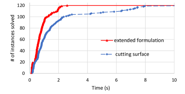
Figure 1. Number of instances solved as a function of time. The cutting surface requires on average 1.79 seconds to solve an instance, and can solve all 120 instances in 13.3 seconds or less. In contrast, the extended formulation (25) requires on average 0.78 seconds, and solves all instances in less than 2.6 seconds.

We also tested the effect of the extended formulation using CPLEX branch-and-bound solver. While we did not encounter numerical issues resulting in incorrect behavior by the solver (the cutting surface method does result in numerical issues, see [7]), the performance of the branch-and-bound method is substantially impaired when using the extended formulation. We discuss in more detail the issues of using the extended formulation with CPLEX branch-and-bound method in the appendix.

4. $\mathcal{NP}$-hardness with bound constraints on continuous variables

The set $\mathcal{Q}$ and its rank-one specialization $\mathcal{Q}_{1}$ studied so far assume that the continuous variables are either unbounded, or non-negative/non-positive. Either way, set $\mathcal{Q}$ and $\mathcal{Q}_{1}$ admit a similar disjunctive form given in Theorem 1 and Proposition 3, respectively. A natural question is whether the addition of bounds on the continuous variables results in similar convexifications, or if the resulting sets are structurally different. In this section, we show that it would be unlikely to find a tractable description of the the convex hulls with bounded variables, unless $\mathcal{P}=\mathcal{NP}$.

Consider the set

$$\mathcal{Q}_{B}\stackrel{{\scriptstyle\mathclap{\text{\tiny def}}}}{{=}}\left\{(t,x,z)\in\mathbb{R}^{n+1}\times\{0,1\}^{n}:t\geq f(x),\;0\leq x\leq z\right\}.$$

We show that optimizing over set $\text{cl conv}(\mathcal{Q}_{B})$ is $\mathcal{NP}$-hard even when $\operatorname{rank}(f)=1$. Two examples are given to illustrate this point – single node flow sets and rank-one quadratic forms.

Single-node fixed-charge flow set

The single-node fixed-charge flow set is the mixed integer linear set defined as

$$\mathcal{T}\stackrel{{\scriptstyle\mathclap{\text{\tiny def}}}}{{=}}\left\{(x,z)\in\mathbb{R}^{n}\times\{0,1\}^{n}:\sum_{i=1}^{n}a_{i}x_{i}\leq b,\;0\leq x\leq z\right\},$$

where $0<a_{i}\leq b\;\forall i\in[n]$. Note that one face of the single-node flow set $\text{conv}(\mathcal{T}\cap\{(x,z):x_{i}=z_{i}\;\forall i\in[n]\})$ is isomorphic to the knapsack set $\text{conv}(\{z\in\{0,1\}^{n}:\sum_{i=1}^{n}a_{i}z_{i}\leq b\})$. If we define $f(x)=g\left(a^{\top}x\right)$, where $g(t)=\delta\left(t;\left\{t\in\mathbb{R}:t\leq b\right\}\right)$, it is clear that $\mathcal{Q}_{B}=\mathbb{R}_{+}\times\mathcal{T}$, which means $\mathcal{T}$ is isomorphic to one facet of $\text{conv}(\mathcal{Q}_{B})$. Since any compact polyhedral description of $\text{conv}(\mathcal{Q}_{B})$ would imply the existence of a polynomial time algorithm to optimize over $\mathcal{T}$, we conclude that such description is not possible unless $\mathcal{P}=\mathcal{NP}$.

Extensions for Rank-one quadratic programs

In this section, we discuss two natural extensions for rank-one quadratic programs. We first consider the extension that box-constraints are added for continuous variables. Specifically, consider the following mixed-integer quadratic program

$$\min_{x,z} \left(a^{\top}x\right)^{2}+b^{\top}x+c^{\top}z$$ (27)

s.t. $$0\leq x\leq z,$$

$$z\in\{0,1\}^{n}.$$

We aim to show (27) is $\mathcal{NP}$-hard in general. To achieve this goal, we show that (27) includes the following well known 0-1 knapsack problem (28) as a special case.

$$\min_{z\in\{0,1\}^{n}} -v^{\top}z$$ (28)

s.t. $$w^{\top}z\leq W,$$

where $(v,w,W)\in\mathbb{Z}_{+}^{2n+1}$ are nonnegative integers such that $w_{i}\leq W\leq\sum_{j}w_{j}\;\forall i\in[n]$.

Proposition 6.

The knapsack problem (28) is equivalent to the optimization problem

$$\min_{x,z} M_{1}\left(Wx_{0}+\sum_{i=1}^{n}w_{i}x_{i}-W\right)^{2}-M_{2}\left(\sum_{i=1}^{n}x_{i}\right)+\sum_{i=1}^{n}(M_{2}-v_{i})z_{i}$$ (29)

s.t. $$0\leq x_{i}\leq z_{i},\;i=0,1,\dots,n$$

$$z_{i}\in\{0,1\},\;i=0,1,\dots,n,$$

where $M_{1}=\sum_{i=1}^{n}v_{i}+1$ and $M_{2}=2nW^{2}M_{1}+1$ are polynomial in the input size.

Proof.

Denote the objective function by $\theta(x,z)$. First, since the objective function does not involve $z_{0}$, $z_{0}$ can be safely taken as $1$. Second, we now show that $M_{2}$ is large enough to force $x_{i}=z_{i}$ for all $i\in[n]$. Specifically, for any $i\in[n]$, since $x_{0},x_{i}\leq 1$ and $w_{i}\leq W$, it holds that

$$\frac{\partial\theta(x,z)}{\partial x_{i}} =2M_{1}w_{i}\left(Wx_{0}+\sum_{i=1}^{n}w_{i}x_{i}-W\right)-M_{2}$$

$$\leq 2nW^{2}M_{1}-M_{2}<0.$$

That is, $\theta(x,z)$ is decreasing with respect to $x_{i},i\in[n]$, which implies $x_{i}=z_{i}$ in any optimal solution. It follows that (29) can be simplified to

$$\min_{x_{0},z} M_{1}\left(Wx_{0}+\sum_{i=1}^{n}w_{i}z_{i}-W\right)^{2}-\sum_{i=1}^{n}v_{i}z_{i}$$ (30)

s.t. $$0\leq x_{0}\leq 1,\;z_{i}\in\{0,1\},\;i=1,\dots,n,$$

Next, we claim that $M_{1}$ is large enough to ensure that the optimal solution to (30) satisfies $Wx_{0}+\sum_{i=1}^{n}w_{i}z_{i}-W=0,$ that is, $x_{0}=1-\left(w^{\top}z\right)/W$. To prove it rigorously, observe that the minimum value of (30) must be non-positive since $x_{0}=1,z=0$ is a feasible solution with objective value equal to $0$. Moreover, since $1-\left(w^{\top}z\right)/W\leq 1$, if $x_{0}\neq 1-\left(w^{\top}z\right)/W$ at the optimal solution to (30), then $1-\left(w^{\top}z\right)/W<0$ and the optimal $x_{0}$ must attain its lower bound $0$. Furthermore, $1-\left(w^{\top}z\right)/W<0$ implies that $w^{\top}z\geq W+1$ since $w,\;W$ and $z$ are nonnegative integers. In this case, setting $x_{0}=0$, the minimum objective value of (30) can be written as

$$M_{1}\left(\sum_{i=1}^{n}w_{i}z_{i}-W\right)^{2}-\sum_{i=1}^{n}v_{i}z_{i}>M_{1}-\sum_{i}v_{i}=1>0,$$

which contradicts the non-positivity of the optimal objective value.

Therefore, we can substitute out $x_{0}=1-\left(w^{\top}z\right)/W$ and (29) further reduces to

$$\min_{z} -\sum_{i=1}^{n}v_{i}z_{i}$$

s.t. $$0\leq 1-\frac{w^{\top}z}{W}\leq 1,$$

$$z_{i}\in\{0,1\},\;i=1,\dots,n,$$

which is equivalent to (28), because $\left(w^{\top}z\right)/W\geq 0$ holds trivially. ∎

Due to the equivalence between optimization problems and separation problems [31], Proposition 6 indicates that it is impossible to extend the analysis in Section 3.1 and Section 3 to the case with bounded continuous variables.

Besides the addition of box-constraints, another natural extension for rank-one quadratic programs is the “rank-one+diagonal” objective. Precisely, consider

$$\min_{x,z} \left(a^{\top}x\right)^{2}+\sum_{i=1}^{n}d_{i}x_{i}^{2}+b^{\top}x+c^{\top}z$$ (31)

s.t. $$x\circ(1-z)=0,$$

$$x\in\mathbb{R}^{n}_{+},\;z\in\{0,1\}^{n},$$

where $a,b,c\in\mathbb{R}^{n}$, $d\in\mathbb{R}^{n}_{+}$, and vector $u\circ v$ represents the Hadamard product of $u$ and $v$, i.e. $(u\circ v)_{i}=u_{i}v_{i}$. Han et al., [34] proves that problem (31) includes the $\mathcal{NP}$-hard subset sum problem as a special case.

Proposition 7 ([34]).

Problem (31) is $\mathcal{NP}$-hard.

For the same reason mentioned above, it is unlikely to get a tractable convex hull description of the corresponding mixed-integer epigraph

$$\left\{(t,x,z)\in\mathbb{R}\times\mathbb{R}_{+}^{n}\times\{0,1\}^{n}:\;t\geq\left(a^{\top}x\right)^{2}+\sum_{i=1}^{n}d_{i}x_{i}^{2},\;x\circ(1-z)=0\right\}.$$

5. Experiments with signal denoising problems

In this section, we test the effectiveness of the low-rank formulations derived in this paper on signal denoising problems. In particular, given noisy observations $c\in\mathbb{R}^{n}$ of a temporal process $X\in\mathbb{R}^{n}$, the goal is to recover the true values of the process. We assume (i) that the temporal process is sparse, i.e., $\|X\|_{0}$ is small; (ii) most observations are noisy realizations of $X$, i.e., $(X_{i}-c_{i})^{2}$ is small; (iii) a small (and unknown) subset $J$ of observations have been subjected to arbitrarily large corruptions, thus the values $c_{j}$ for $j\in J$ can be arbitrarily far from $X_{j}$. The problem of inferring the true values of the process $X$ can be mathematically formulated as

$$\min_{x,v,z,w} \sum_{i=1}^{n}(x_{i}-v_{i}-c_{i})^{2}+\Omega\sum_{i=\ell+1}^{n}\left(x_{i}-\sum_{j=1}^{\ell}\alpha^{j}x_{i-\ell+j-1}\right)^{2}$$ (32)

s.t. $$x\circ(1-z)=0,\;\sum_{i=1}^{n}z_{i}\leq k_{1},\;z\in\{0,1\}^{n}$$

$$v\circ(1-w)=0,\;\sum_{i=1}^{n}w_{i}\leq k_{2},\;w\in\{0,1\}^{n},$$

where $k_{1}$ is the estimated number of nonzero elements in the true signal, $k_{2}$ is the maximum number of outliers in data $c$, $\Omega>0$ is the weight of the smoothness part in the objective, $0<\alpha<1$, and $\ell$ is the length of the convolution kernel.

Note that the objective function consists of two parts – the first sum encodes the fitness of the estimator to the observations; the second sum incorporates the smoothness prior of the true signal that the current signal value $x_{i}$ is assumed to be similar to those incurred before the time stamp $i$ and the proximity decays in temporal distance at rate $\alpha$. Observe that $w_{i}$ indicates whether the observation $i$ is an outlier. Indeed, if $w_{i}=0$, then $v_{i}=0$ by the complementarity constraint $v_{i}(1-w_{i})=0$ and $c_{i}$ is used in (32). On the other hand, if $w_{i}=1$, then at the optimal solution one must have $v_{i}=x_{i}-c_{i}$. In this case, $c_{i}$ plays no role in the objective and datapoint $i$ is thus discarded as an outlier.

We point out that problem (32) is closely related to several problems in the literature. On one hand, if $\ell=1$ and $\alpha=1$, then the smoothness terms reduce to $(x_{i}-x_{i-1})^{2}$. In this case, problems with sparse signals and no outliers (i.e., $k_{2}=n$) where considered in [8], and problems with outliers but no sparsity (i.e., $k_{1}=n$) were considered in [28]. Moreover, if $\ell=1$, then the penalized version of (32), where cardinality constraints on sparsity and outliers are replaced with fixed costs, is polynomial-time solvable [35]. On the other hand, if the width $\ell$ is large and terms $\alpha^{j}$ are replaced with arbitrary constants, then (32) is closely related with sparse/robust versions of linear regression. In particular, there have been several recent papers related to sparse linear regression [6, 16, 21, 36, 51], but relatively few mixed-integer optimization approaches for problems with outliers [53, 54] or both outliers and sparsity [39].

5.1. Instance generation

In this section, we describe how we generate test instances. Set $\alpha=0.9$, $k_{1}=3n/50$ and $k_{2}=n/100$. The noised signal $c$ is produced in the following way:

1. Initially, $c=0$

2. Repeat the following process to generate $s=n/50$ “spikes” of the signal with each spike consisting of $h=5$ non-zero values

   1. Select an index $i_{0}$ uniformly between 1 and $n+1-h$ as the starting position of a given spike.

   2. Draw an vector $v\in\mathbb{R}^{h}$ from a multivariate normal distribution $\mathcal{N}(0,\Sigma)$, where $\Sigma$ is the covariate matrix with $\Sigma_{ij}=\frac{i(h+1-j)}{h+1}$.

   3. Update $c_{i_{0}+i}\leftarrow c_{i_{0}+i}+v_{i},\;i=1,\dots,h$.

3. Add a Gaussian noise $c\leftarrow c+0.2\varepsilon$, where $\varepsilon\in\mathbb{R}^{n}$ is sample from the standard multivariate normal distribution $\mathcal{N}(0,I)$. Then normalize the data $c\leftarrow c/\left\|c\right\|_{\infty}$.

4. Corrupt the data $c$ by repeating the following process $k_{2}$ times

   1. Select an index $i$ uniformly between 1 and $n$.

   2. Update $c_{i}\leftarrow c_{i}+4\epsilon$, where $\epsilon$ is drawn from the standard normal distribution.

All experiments in this section are conducted using Gurobi 9.0 solver with default settings on a laptop with a 2.30GHz $\text{Intel}^{\text{\textregistered}}$ $\text{Core}^{\text{\tiny TM}}$ i9-9880H CPU and 64 GB main memory. The time limit is set as 600 seconds.

5.2. Formulations

Three mixed-integer reformulations of (32) are implemented and compared - $\mathsf{Basic}$, $\mathsf{RankOne}$, and $\mathsf{RankTwo}$.

5.2.1. $\mathsf{Basic}$

In $\mathsf{Basic}$, we reformulate the complementarity constraints using big-M formulations where $M=10^{4}$

$$\min_{x,v,z,w} \sum_{i=1}^{n}(x_{i}-v_{i}-c_{i})^{2}+\Omega\sum_{i=\ell+1}^{n}\left(x_{i}-\sum_{j=1}^{\ell}\alpha^{j}x_{i-\ell+j-1}\right)^{2} \mathsf{Basic}$$ ()

s.t. $$-Mz\leq x\leq Mz,\;\sum_{i}z_{i}\leq k_{1},\;z\in\{0,1\}^{n}$$

$$-Mw\leq v\leq Mw,\;\sum_{i}w_{i}\leq k_{2},\;w\in\{0,1\}^{n}.$$

We comment that the continuous relaxation of $\mathsf{Basic}$ –the optimization problem obtained by dropping the integrality constraints of $x$ and $w$– always yields a trivial optimal value $0$. Indeed, since $M$ is sufficiently large, one can take $v=c$, $x=z=0$ and $w=v/M$ as a feasible solution to the relaxation of $\mathsf{Basic}$ whose objective is simply $0$.

5.2.2. $\mathsf{RankOne}$

In $\mathsf{RankOne}$, each individual fitness term and smoothness term in (32) are replaced with the conic representation of the rank-one formulation suggested by Proposition 4

$$\min_{x,v,z,w} \sum_{i=1}^{n}t_{i}+\Omega\sum_{i=\ell+1}^{n}s_{i}-2\sum_{i=1}^{n}c_{i}(x_{i}-v_{i})+\left\|c\right\|_{2}^{2} \mathsf{RankOne}$$ ()

s.t. $$t_{i}\geq(x_{i}-v_{i})^{2},\;t_{i}(z_{i}+w_{i})\geq(x_{i}-v_{i})^{2} i=1,\dots,n$$

$$s_{i}\geq\left(x_{i}-\sum_{j=1}^{\ell}\alpha^{j}x_{i-\ell+j-1}\right)^{2} i=\ell+1,\dots,n$$

$$s_{i}\left(\sum_{j=i-\ell}^{i}z_{j}\right)\geq\left(x_{i}-\sum_{j=1}^{\ell}\alpha^{j}x_{i-\ell+j-1}\right)^{2} i=\ell+1,\dots,n$$

$$-Mz\leq x\leq Mz,\;\sum_{i}z_{i}\leq k_{1},\;z\in\{0,1\}^{n}$$

$$-Mw\leq v\leq Mw,\;\sum_{i}w_{i}\leq k_{2},\;w\in\{0,1\}^{n}.$$

5.2.3. $\mathsf{RankTwo}$

In $\mathsf{RankTwo}$, for each $i=1,\dots,\ell$, we replace the $i^{\text{th}}$ fitness term with its rank-one strengthening. For each $i=\ell+1,\dots,n$, we combine the $i^{\text{th}}$ fitness and smoothness term and replace their sum with the rank-two strengthening. Specifically, define the rank-two mixed-integer set

$$\mathcal{Q}_{2}=\left\{(t,x,z,v,w,y,u):\begin{aligned} &t\geq(y-v)^{2}+\Omega\left(y-\sum_{i=1}^{\ell}x_{i}\right)^{2}\\ &x\circ(1-z)=0,\;v(1-w)=0,\;y(1-u)=0\\ &z\in\{0,1\}^{\ell},w\in\{0,1\},u\in\{0,1\}\end{aligned}\right\}.$$

The description of $\text{cl conv}\mathcal{(}Q_{2})$ in the lifted space can be readily derived from Theorem 1 using disjunctive programming techniques, which we give in Proposition 8 in the appendix. Then $\mathsf{RankTwo}$ is given as

$$\min_{x,v,z,w} \sum_{i=1}^{n}t_{i}-2\sum_{i=1}^{n}c_{i}(x_{i}-v_{i})+\left\|c\right\|_{2}^{2} \mathsf{RankTwo}$$ ()

s.t. $$t_{i}\geq(x_{i}-v_{i})^{2},t_{i}(z_{i}+w_{i})\geq(x_{i}-v_{i})^{2} i=1,\dots,\ell$$

$$(t_{i},a\circ x_{(i-\ell):(\ell-1)},z_{(i-\ell):(\ell-1)},v_{i},w_{i},x_{i},z_{i})\in\text{cl conv}(\mathcal{Q}_{2}) i=\ell+1,\dots,n$$

$$-Mz\leq x\leq Mz,\;\sum_{i}z_{i}\leq k_{1},\;z\in\{0,1\}^{n}$$

$$-Mw\leq v\leq Mw,\;\sum_{i}w_{i}\leq k_{2},\;w\in\{0,1\}^{n},$$

where $x_{i:j}$ represents the subvector of $x$ indexed from $i$ to $j$ and $a=(\alpha^{\ell},\alpha^{\ell-1},\dots,\alpha)$.

5.3. Results

Each row of Table 1 and Table 2 shows an average statistics over five instances with the same parameters. The tables display the dimension of the problem $n$, the initial gap (IGap), the solution time for solving the corresponding mixed-integer formulation (Time), the end gap provided by the solver at termination (EGap), the number of nodes explored by the solver (Nodes), the number of instances solved to optimality within the time limit (#), and the root improvement of $\mathsf{RankTwo}$ compared with $\mathsf{Basic}$ (RI-basic) and $\mathsf{RankOne}$ (RI-rankOne). The initial gap is computed as $\text{IGap}=\frac{\text{obj}_{\text{best}}-\text{obj}_{\text{cont}}}{|\text{obj}_{\text{best}}|}\times 100$, where $\text{obj}_{\text{best}}$ is the objective value of the feasible solution found and $\text{obj}_{\text{cont}}$ represents the objective value of the continuous relaxation, that is, obtained by relaxing $\{0,1\}^{n}$ to $[0,1]^{n}$ in the three formulations. The root improvement is computed as $\text{RI-basic}=\frac{\text{obj}_{\text{rankTwo}}-\text{obj}_{\text{basic}}}{\text{obj}_{\text{best}}-\text{obj}_{\text{basic}}}\times 100$, where $\text{obj}_{\text{rankTwo}}$ is the objective value of the convex relaxation of $\mathsf{RankTwo}$ and where $\text{obj}_{\text{basic}}$ is the objective value of the convex relaxation of $\mathsf{Basic}$. The computation of RI-rankOne is similar. Finally, we remark that the initial gap of $\mathsf{Basic}$ is not reported because it is always nearly 0, which is expected and explained above.

Table 1 displays the computational results for varying $\ell\in\{1,2,5\}$ and fixed $\Omega=0.05$. As we expect, $\mathsf{Basic}$ has the worst performance and can only solve three instances in the low-dimensional setting $n=100$. On the other hand, $\mathsf{RankTwo}$ is able to solve almost all instances to optimality when $\ell=1,2$ by exploring much less nodes in the branch-and-bound tree regardless of the problem dimension. The root improvement of $\mathsf{RankTwo}$ over $\mathsf{Basic}$ is significant in all settings. The performance of $\mathsf{RankOne}$ is in the middle of $\mathsf{Basic}$ and $\mathsf{RankTwo}$ - it can solve all instances in low-dimension settings and none when $n=200,300$. In addition, RI-rankOne ranges from $8\%$ to $50\%$ and achieves the best $50\%$ as $\ell=2$ and $n=100$. Table 2 displays the computational results for fixed $\ell=2$ and varying $\Omega\in\{0.01,0.05,0.25,0.5\}$. The conclusions we can draw from Table 2 are similar to the ones from Table 1. It is worthing noting that in the case where a certain instance can be solved by both $\mathsf{RankOne}$ and $\mathsf{RankTwo}$, the solution time of $\mathsf{RankOne}$ outperforms $\mathsf{RankTwo}$. However, many instances that are not solvable using $\mathsf{RankOne}$ can be solved by $\mathsf{RankTwo}$ especially in more difficult settings. In summary, we conclude that $\mathsf{RankTwo}$ is preferable to utilizing for challenging instances of the signal denoising problem (32).

The computational profile of three formulations on all 105 instances is presented in Figure 2. Among them, $\mathsf{RankOne}$ successfully solves 41 instances in 600 seconds. In comparison, $\mathsf{RankTwo}$ is able to solve the same number of instances in 5.7 seconds, which is two orders of magnitude faster than $\mathsf{RankOne}$. Furthermore, $\mathsf{RankTwo}$ surpasses $\mathsf{RankOne}$ by solving 81 instances within the given time limit, which is approximately twice the number of instances solved by $\mathsf{RankOne}$. Overall, these findings demonstrate the superior performance of $\mathsf{RankTwo}$ relative to $\mathsf{RankOne}$ in terms of solvability.

6. Conclusions

In this paper, we propose a new disjunctive programming representation of the convex envelope of a low-rank convex function with indicator variables and complementary constraints. The ensuing formulations are substantially more compact than alternative disjunctive programming formulations. As a result, it is substantially easy to project out the additional variables to recover formulations in the original space of variables, and to implement the formulations using off-the-shelf solvers. Moreover, the computational results evidently demonstrate the efficacy of the proposed formulations when applied to well-structured problems, particularly in problems where the low rank functions are involving few variables as well.

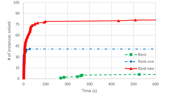
Figure 2. Number of instances solved as a function of time

Table 1. Varying kernel width $\ell$ and fixed $\Omega=0.05$

$n$	$\ell$	$\mathsf{Basic}$				$\mathsf{RankOne}$					$\mathsf{RankTwo}$
		EGap	Time	Nodes	#	IGap	EGap	Time	Nodes	#	IGap	EGap	Time	Nodes	#	RI-basic	RI-rankOne
100	1	49.00	447	180,297	2	4.30	0.00	1.13	342	5	2.09	0.00	1.65	7.8	5	97.91	50.37
100	2	54.40	585	182,314	1	5.68	0.00	1.36	131	5	4.22	0.00	1.51	3.8	5	95.78	26.02
100	5	61.01	600	39,610	0	8.99	0.00	2.91	344	5	7.21	0.00	5.60	16.8	5	92.79	20.42
200	1	43.30	600	3,394	0	3.91	3.03	600	9,279	0	2.07	0.00	23.5	155	5	97.93	48.08
200	2	51.22	600	3,391	0	10.36	9.45	600	6,610	0	8.18	0.00	32.3	102.8	5	91.82	21.31
200	5	56.95	600	3,688	0	10.82	10.31	600	7,986	0	9.70	10.91	600	531	0	90.30	11.13
300	1	82.17	600	3,149	0	4.78	7.94	600	3,414	0	2.50	0.00	23.4	58	5	97.50	48.82
300	2	87.06	600	4,288	0	8.70	10.09	600	2,701	0	7.18	4.02	141	311	4	92.82	17.99
300	5	94.55	600	2,520	0	17.33	18.31	600	2,766	0	16.00	31.18	600	292.4	0	84.00	8.68

Table 2. Varying $\Omega$ and fixed kernel-width $\ell=2$

$n$	$\Omega$	$\mathsf{Basic}$				$\mathsf{RankOne}$					$\mathsf{RankTwo}$
		EGap	Time	Nodes	#	IGap	EGap	Time	Nodes	#	IGap	EGap	Time	Nodes	#	RI-basic	RI-rankOne
100	0.01	94.42	600	146,503	0	1.38	0.00	1.32	159	5	0.90	0.00	1.67	3	5	99.10	35.50
100	0.05	26.61	446	50,971	2	7.31	0.00	1.22	253	5	4.92	0.00	1.95	8	5	95.08	32.67
100	0.25	41.19	600	65,345	0	17.50	0.00	1.76	740	5	13.33	0.00	5.41	36	5	86.67	25.46
100	0.50	18.18	532	70,338	1	28.99	0.00	2.96	1,056	5	24.14	0.00	4.21	23	5	75.86	17.01
200	0.01	34.31	600	4,653	0	1.92	0.00	9.98	1,438	5	1.43	0.00	5.81	11	5	98.57	26.23
200	0.05	42.16	600	4,811	0	7.01	5.55	600	7,430	0	5.27	0.75	134	244	4	94.73	25.56
200	0.25	61.65	600	3,262	0	20.11	20.25	600	6,573	0	15.60	3.72	217	579	4	84.40	23.02
200	0.50	75.17	600	3,414	0	30.80	29.86	600	6,092	0	24.38	17.77	484	614	1	75.62	22.39
300	0.01	78.96	600	2,785	0	1.65	1.76	486	4,120	1	1.15	0.00	29.3	51	5	98.85	30.19
300	0.05	87.16	600	2,959	0	7.85	10.74	600	2,844	0	5.77	0.00	122	339	5	94.23	26.58
300	0.25	80.01	600	3,192	0	20.46	20.87	600	2,780	0	16.12	15.93	368	369	2	83.88	21.79
300	0.50	87.68	600	3,265	0	31.09	31.80	600	2,485	0	25.20	25.51	488	543	1	74.80	19.17

Appendix A On computational experiments with branch-and-bound

As mentioned in §3.4, the extended formulation (25) did not produce good results when used in conjunction with CPLEX branch-and-bound solver. To illustrate this phenomenon, Table 3 shows details on the performance of the solver in a single representative instance, but similar behavior was observed in all instances tested. The table shows from left to right: the time required to solve the convex relaxation via interior point methods and the lower bound produced by this relaxation (note that this is not part of the branch-and-bound algorithm); the time required to process the root node of the branch-and-bound tree, and the corresponding lower bound obtained; the time used to process the branch-and-bound tree, the number of branch-and-bound nodes explored, and the lower bound found after processing the tree (we set a time limit of 10 minutes).

Table 3. Performance of CPLEX solver in an instance with $n=500$ and $k=10$. Default settings are used, and a time limit of 10 minutes is set. The optimal objective value in the particular instance is 1.47.

Method	Convex relaxation		Root node		Branch-and-bound
	Time(s)	LB	Time(s)	LB	Time(s)	Nodes	LB
Without (25)	0.2	1.09	3.5	1.20	7.7	460	1.47
With (25)	2.4	1.30	45.9	0.90	600	4,073	0.99

Our expectations a priori were as follows: using inequalities (25) should result in harder convex relaxations solved, and thus less nodes explored within a given time limit; on the other hand, due to improved relaxations and higher-quality lower bounds, the algorithm should be able to prove optimality after exploring substantially less nodes. Thus, there should be a tradeoff between the number of nodes to be explored and the time required to process each node. From Table 3, we see that there is no tradeoff in practice.

The performance of the solver without inequalities (25) is as expected. While just solving the convex relaxation via interior point methods requires 0.2 seconds, there is an overhead of 3 seconds to process the root node due to preprocessing/cuts/heuristics and additional methods used by the solver (and the quality of the lower bound at the root node is slightly improved as a result).Then, after an additional 4 seconds used to explore 460 nodes, optimality is proven.

The performance of the solver using inequalities (25) defied our expectations. In theory, the more difficult convex relaxation can be solved with an overhead of 2 seconds, resulting in a root improvement of $(1.30-1.09)/(1.47-1.09)=55.3\%$ (better than the one achieved by default CPLEX). In practice, the overhead is 40 seconds, and results in a degradation of the relaxation, that is, the lower bound proved at the root node is worse than the natural convex relaxation of problem without inequalities (25). From that point out, the branch-and-bound progresses slowly due to the more difficult relaxations, and the lower bounds are worse throughout the tree. Even after the time limit of 10 minutes and over 4,000 nodes explored, the lower bound proved by the algorithm is still worse than the natural convex relaxation.

While we cannot be sure about the exact reason of this behavior, we now make an educated guess. Most conic quadratic branch-and-bound solvers such as CPLEX do not use interior point methods to solve relaxations at each node of the branch-and-bound tree, but rather rely on polyhedral outer approximations in an extended space to benefit from the warm-start capabilities of the simplex method. We conjecture that while formulation (25) might not be particularly challenging to solve via interior point methods, it might be difficult to construct a good-quality outer approximation of reasonable size. If so, then the actual relaxation used by the solver is possibly a poor-quality linear outer approximation of the feasible region induced by (25), and is still difficult to solve, resulting in the worst of both worlds. We point out that the second author has encountered similar counterintuitive behavior with solvers (other than CPLEX) based on linear outer approximations [4]. We also attempted that setting the MIQCP strategy switch (parameter MIQCPStrat) to one, which “tells CPLEXs to solve a QCP relaxation of the model at each node”. However, in such cases, the optimization terminates with numerical issues in most cases.

Appendix B Convex hull description of $\mathcal{Q}_{2}$

In this section, we give the convex hull description of $\mathcal{Q}_{2}$ in the lifted space. We first prove a lemma to simplify the notation. Consider

$$\mathcal{S}_{i}=\left\{(t,x,z):t\geq f_{i}(x_{\mathcal{I}_{i}}),\;z_{j}=1\;\forall j\in\mathcal{I}_{i},\;x_{j}=0,z_{j}\in\{0,1\}\;\forall j\not\in\mathcal{I}_{i}\right\}\;i\in[n],$$

where each $\mathcal{I}_{i}\subseteq[n]$ and $f_{i}$ is a closed convex function with $f_{i}(0)=0$.

Lemma 5.

Let $\mathcal{S}=\bigcup_{i}\mathcal{S}_{i}$. A point $(t,x,z)\in\text{cl conv}\mathcal{S}$ if and only if the following system is consistent

$$t=\sum_{i}t_{i}$$

$$t_{i}\geq f^{\pi}(x^{i}_{\mathcal{I}_{i}};\lambda_{i}) \forall i\in[n]$$

$$x_{i}=\sum_{j:i\in\mathcal{I}_{j}}x^{j}_{i} \forall i\in[n]$$

$$\sum_{j:i\in\mathcal{I}_{j}}\lambda_{j}\leq z_{i}\leq 1 \forall i\in[n]$$

$$\lambda\geq 0,\sum_{i\in[n]}\lambda_{i}=1.$$

Proof.

Using disjunctive programming techniques, one can see that $(t,x,z)\in\text{cl conv}\mathcal{S}$ if and only if the following system is consistent

$$t=\sum_{i}t_{i}$$

$$x_{i}=\sum_{j}x^{j}_{i},\;z_{i}=\sum_{j}z^{j}_{i} \forall i\in[n]$$

$$x_{j}^{i}=0,z_{j}^{i}\in[0,\lambda_{i}]\; \forall j\notin\mathcal{I}_{i},\forall i\in[n]$$

$$z_{j}^{i}=\lambda_{i}\; \forall j\in\mathcal{I}_{i},\forall i\in[n]$$

$$t_{i}\geq f^{\pi}(x^{i}_{\mathcal{I}_{i}};\lambda_{i}) \forall i\in[n]$$

$$\lambda\geq 0,\sum_{i\in[n]}\lambda_{i}=1.$$

First observe that one can easily substitute out $x^{i}_{j}\;\forall j\notin\mathcal{I}_{i}$ and $z^{i}_{j}\;\forall j\in\mathcal{I}_{i}$ in above expression. What is more, since for each $j\notin\mathcal{I}_{i}$, $z_{j}^{i}\in[0,\lambda_{i}]$ is independent of all other variables except $z_{i}$ and $\lambda_{i}$. Thus, one can use Fourier-Motzkin eliminating to substitute such $z_{j}^{i}$ with their bounds, which gives the upper bound of $z_{i}\leq\sum_{i}\lambda_{i}=1$. ∎

Recall the definition of

$$\mathcal{Q}_{2}=\left\{(t,x,z,v,w,y,u):\begin{aligned} &t\geq(y-v)^{2}+\Omega\left(y-\sum_{i=1}^{\ell}x_{i}\right)^{2}\\ &x\circ(1-z)=0,\;v(1-w)=0,\;y(1-u)=0\\ &x\in\mathbb{R}^{\ell},z\in\{0,1\}^{\ell},w\in\{0,1\},u\in\{0,1\}\end{aligned}\right\}.$$

Proposition 8.

The closed convex hull of $\mathcal{Q}_{2}$ is given by the following extended formulation

$$t\geq\sum_{i}(t^{\mathcal{V}_{i}}+t^{\mathcal{V}_{iy}}+t^{\mathcal{V}_{iv}})+t^{\mathcal{V}_{y}}+t^{\mathcal{V}_{v}}+t^{\mathcal{V}_{yv}}$$

$$x_{i}=x^{\mathcal{V}_{i}}_{i}+x_{i}^{\mathcal{V}_{iy}}+x_{i}^{\mathcal{V}_{iv}}+x_{i}^{\mathcal{R}} i\in[\ell]$$

$$y=y^{\mathcal{V}_{y}}+\sum_{i=1}^{\ell}y^{\mathcal{V}_{iy}}+y^{\mathcal{V}_{yv}}+y^{\mathcal{R}}$$

$$v=v^{\mathcal{V}_{v}}+\sum_{i=1}^{\ell}v^{\mathcal{V}_{iv}}+v^{\mathcal{V}_{yv}}+v^{\mathcal{R}}$$

$$y^{\mathcal{R}}=v^{\mathcal{R}}=\sum_{i=1}^{\ell}x_{i}^{\mathcal{R}}$$

$$\lambda^{\mathcal{V}_{i}}+\lambda^{\mathcal{V}_{iy}}+\lambda^{\mathcal{V}_{iv}}+\lambda^{\mathcal{R}}\leq z_{i}\leq 1 \forall i\in[\ell]$$

$$\lambda^{\mathcal{V}_{y}}+\sum_{i=1}^{\ell}\lambda^{\mathcal{V}_{iy}}+\lambda^{\mathcal{V}_{yv}}+\lambda^{\mathcal{R}}\leq u\leq 1$$

$$\lambda^{\mathcal{V}_{v}}+\sum_{i=1}^{\ell}\lambda^{\mathcal{V}_{iv}}+\lambda^{\mathcal{V}_{yv}}+\lambda^{\mathcal{R}}\leq w\leq 1$$

$$\sum_{i}\lambda^{\mathcal{V}_{i}}+\sum_{i}\lambda^{\mathcal{V}_{iy}}+\sum_{i}\lambda^{\mathcal{V}_{iv}}+\lambda^{\mathcal{V}_{y}}+\lambda^{\mathcal{V}_{v}}+\lambda^{\mathcal{V}_{yv}}+\lambda^{\mathcal{V}_{R}}\leq 1,\;\lambda\geq 0$$

$$t^{\mathcal{V}_{i}}\lambda^{\mathcal{V}_{i}}\geq\Omega\left(x^{\mathcal{V}_{i}}\right)^{2} \forall i\in[\ell]$$

$$t^{\mathcal{V}_{y}}\lambda^{\mathcal{V}_{y}}\geq(1+\Omega)\left(y^{\mathcal{V}_{y}}\right)^{2}$$

$$t^{\mathcal{V}_{v}}\lambda^{\mathcal{V}_{v}}\geq\left(v^{\mathcal{V}_{v}}\right)^{2}$$

$$t^{\mathcal{V}_{iy}}\lambda^{\mathcal{V}_{iy}}\geq\left(y^{\mathcal{V}_{iy}}\right)^{2}+\Omega\left(y^{\mathcal{V}_{iy}}-x_{i}^{\mathcal{V}_{iy}}\right)^{2} \forall i\in[\ell]$$

$$t^{\mathcal{V}_{iv}}\lambda^{\mathcal{V}_{iv}}\geq\left(v^{\mathcal{V}_{iv}}\right)^{2}+\Omega\left(x_{i}^{\mathcal{V}_{iv}}\right)^{2} \forall i\in[\ell]$$

$$t^{\mathcal{V}_{yv}}\lambda^{\mathcal{V}_{yv}}\geq(y^{\mathcal{V}_{yv}}-v^{\mathcal{V}_{yv}})^{2}+\Omega\left(y^{\mathcal{V}_{yv}}\right)^{2}$$

Proof.

Define

$$\mathcal{R}=\left\{(t,x,z,v,w,y,u):t\geq 0,y-v=0,y=\sum_{j}x_{j},z_{i}=w=u=1\;\forall j\right\}$$

$$\mathcal{V}_{0}=\left\{(t,x,z,v,w,y,u):\begin{aligned} &t\geq 0,x_{j}=0,z_{j}\in\{0,1\}\;\forall j,\\ &v=y=0,w,u\in\{0,1\}\end{aligned}\right\}$$

$$\mathcal{V}_{i}=\left\{(t,x,z,v,w,y,u):\begin{aligned} &t\geq\Omega x_{i}^{2},\;z_{i}=1,\\ &v=y=0,w,u\in\{0,1\},x_{j}=0,z_{j}\in\{0,1\}\;\forall j\neq i\end{aligned}\right\} \forall i\in[\ell]$$

$$\mathcal{V}_{y}=\left\{(t,x,z,v,w,y,u):\begin{aligned} &t\geq(1+\Omega)y^{2},u=1,\\ &v=0,w\in\{0,1\},x_{j}=0,z_{j}\in\{0,1\}\;\forall j\end{aligned}\right\}$$

$$\mathcal{V}_{v}=\left\{(t,x,z,v,w,y,u):t\geq v^{2},w=1,y=x_{j}=0,u,z_{j}\in\{0,1\}\;\forall j\right\}$$

$$\mathcal{V}_{yv}=\left\{(t,x,z,v,w,y,u):\begin{aligned} &t\geq y^{2}+\Omega(y-x_{i})^{2},z_{i}=u=1,\\ &v=0,w\in\{0,1\},x_{j}=0,z_{j}\in\{0,1\}\;\forall j\neq i\end{aligned}\right\}$$

$$\mathcal{V}_{iy}=\left\{(t,x,z,v,w,y,u):\begin{aligned} &t\geq y^{2}+\Omega(y-x_{i})^{2},z_{i}=u=1,\\ &v=0,w\in\{0,1\},x_{j}=0,z_{j}\in\{0,1\}\;\forall j\neq i\end{aligned}\right\} \forall i\in[\ell]$$

$$\mathcal{V}_{iv}=\left\{(t,x,z,v,w,y,u):\begin{aligned} &t\geq v^{2}+\Omega x_{i}^{2},w=z_{i}=1,\\ &y=0,u\in\{0,1\},x_{j}=0,z_{j}\in\{0,1\}\;\forall j\neq i\end{aligned}\right\}. \forall i\in[\ell]$$

For a general rank-two set, Theorem 1 suggest using $\mathcal{O}\left(n^{2}\right)$ of pieces to describe its closed convex hull. However, for this special set $\mathcal{Q}_{2}$, carefully checking the proof of Theorem 1 we find that that the above defined pieces are sufficient, i.e.

$$\text{cl conv}\mathcal{Q}_{2}=\text{cl conv}\left(\mathcal{V}_{0}\bigcup_{i}\mathcal{V}_{i}\bigcup\mathcal{V}_{y}\bigcup\mathcal{V}_{v}\bigcup\mathcal{V}_{yv}\bigcup_{i}\mathcal{V}_{iy}\bigcup_{i}\mathcal{V}_{iv}\bigcup\mathcal{R}\right).$$

The conclusion follows by applying Lemma 5 to the above disjunction and eliminating the variables associated with $\mathcal{V}_{0}$. Note that we use superscripts to indicates the piece associated with a certain additional variable in the extended formula of $\text{cl conv}\mathcal{Q}_{2}$. ∎

Finally, we note that the number of additional variables used in Proposition 8 is of order $\mathcal{O}\left(\ell\right)$.

References

- Aktürk et al., [2009] Aktürk, M. S., Atamtürk, A., and Gürel, S. (2009). A strong conic quadratic reformulation for machine-job assignment with controllable processing times. Operations Research Letters, 37:187–191.
- Anderson et al., [2019] Anderson, R., Huchette, J., Tjandraatmadja, C., and Vielma, J. P. (2019). Strong mixed-integer programming formulations for trained neural networks. In International Conference on Integer Programming and Combinatorial Optimization, pages 27–42. Springer.
- Anstreicher and Burer, [2021] Anstreicher, K. M. and Burer, S. (2021). Quadratic optimization with switching variables: the convex hull for . Mathematical Programming, 188(2):421–441.
- Atamtürk and Gómez, [2018] Atamtürk, A. and Gómez, A. (2018). Strong formulations for quadratic optimization with M-matrices and indicator variables. Mathematical Programming, 170:141–176.
- Atamturk and Gomez, [2019] Atamturk, A. and Gomez, A. (2019). Rank-one convexification for sparse regression. arXiv preprint arXiv:1901.10334.
- Atamturk and Gómez, [2020] Atamturk, A. and Gómez, A. (2020). Safe screening rules for l0-regression from perspective relaxations. In International conference on machine learning, pages 421–430. PMLR.
- Atamtürk and Gómez, [2022] Atamtürk, A. and Gómez, A. (2022). Supermodularity and valid inequalities for quadratic optimization with indicators. Mathematical Programming, pages 1–44.
- Atamtürk et al., [2021] Atamtürk, A., Gomez, A., and Han, S. (2021). Sparse and smooth signal estimation: Convexification of l0-formulations. Journal of Machine Learning Research, 22(52):1–43.
- Balas, [1979] Balas, E. (1979). Disjunctive programming. Annals of discrete mathematics, 5:3–51.
- Balas, [1985] Balas, E. (1985). Disjunctive programming and a hierarchy of relaxations for discrete optimization problems. SIAM Journal on Algebraic Discrete Methods, 6(3):466–486.
- Balas, [1998] Balas, E. (1998). Disjunctive programming: Properties of the convex hull of feasible points. Discrete Applied Mathematics, 89(1-3):3–44.
- Balas, [2018] Balas, E. (2018). Disjunctive programming. Springer.
- Balas et al., [1989] Balas, E., Tama, J. M., and Tind, J. (1989). Sequential convexification in reverse convex and disjunctive programming. Mathematical Programming, 44(1):337–350.
- Bernal and Grossmann, [2021] Bernal, D. E. and Grossmann, I. E. (2021). Convex mixed-integer nonlinear programs derived from generalized disjunctive programming using cones. arXiv preprint arXiv:2109.09657.
- Bertsimas et al., [2022] Bertsimas, D., Cory-Wright, R., and Pauphilet, J. (2022). Mixed-projection conic optimization: A new paradigm for modeling rank constraints. Operations Research, 70(6):3321–3344.
- Bertsimas et al., [2016] Bertsimas, D., King, A., Mazumder, R., et al. (2016). Best subset selection via a modern optimization lens. The Annals of Statistics, 44:813–852.
- Bienstock, [1996] Bienstock, D. (1996). Computational study of a family of mixed-integer quadratic programming problems. Mathematical programming, 74(2):121–140.
- Bonami, [2011] Bonami, P. (2011). Lift-and-project cuts for mixed integer convex programs. In International Conference on Integer Programming and Combinatorial Optimization, pages 52–64. Springer.
- Ceria and Soares, [1999] Ceria, S. and Soares, J. (1999). Convex programming for disjunctive convex optimization. Mathematical Programming, 86(3):595–614.
- Çezik and Iyengar, [2005] Çezik, M. T. and Iyengar, G. (2005). Cuts for mixed 0-1 conic programming. Mathematical Programming, 104:179–202.
- Cozad et al., [2014] Cozad, A., Sahinidis, N. V., and Miller, D. C. (2014). Learning surrogate models for simulation-based optimization. AIChE Journal, 60(6):2211–2227.
- Dantzig, [1972] Dantzig, G. B. (1972). Fourier-motzkin elimination and its dual. Technical report, STANFORD UNIV CA DEPT OF OPERATIONS RESEARCH.
- De Rosa and Khajavirad, [2022] De Rosa, A. and Khajavirad, A. (2022). Explicit convex hull description of bivariate quadratic sets with indicator variables. arXiv preprint arXiv:2208.08703.
- Dong et al., [2015] Dong, H., Chen, K., and Linderoth, J. (2015). Regularization vs. relaxation: A conic optimization perspective of statistical variable selection. arXiv preprint arXiv:1510.06083.
- Dong and Linderoth, [2013] Dong, H. and Linderoth, J. (2013). On valid inequalities for quadratic programming with continuous variables and binary indicators. In Goemans, M. and Correa, J., editors, Integer Programming and Combinatorial Optimization, pages 169–180, Berlin, Heidelberg. Springer Berlin Heidelberg.
- Frangioni and Gentile, [2006] Frangioni, A. and Gentile, C. (2006). Perspective cuts for a class of convex 0–1 mixed integer programs. Mathematical Programming, 106(2):225–236.
- Frangioni et al., [2019] Frangioni, A., Gentile, C., and Hungerford, J. (2019). Decompositions of semidefinite matrices and the perspective reformulation of nonseparable quadratic programs. Mathematics of Operations Research.
- [28] Gómez, A. (2021a). Outlier detection in time series via mixed-integer conic quadratic optimization. SIAM Journal on Optimization, 31(3):1897–1925.
- [29] Gómez, A. (2021b). Strong formulations for conic quadratic optimization with indicator variables. Mathematical Programming, 188(1):193–226.
- Grossmann, [2002] Grossmann, I. E. (2002). Review of nonlinear mixed-integer and disjunctive programming techniques. Optimization and engineering, 3(3):227–252.
- Grötschel et al., [1981] Grötschel, M., Lovász, L., and Schrijver, A. (1981). The ellipsoid method and its consequences in combinatorial optimization. Combinatorica, 1:169–197.
- Günlük and Linderoth, [2010] Günlük, O. and Linderoth, J. (2010). Perspective reformulations of mixed integer nonlinear programs with indicator variables. Mathematical Programming, 124:183–205.
- Han and Gómez, [2021] Han, S. and Gómez, A. (2021). Single-neuron convexification for binarized neural networks. http://www.optimization-online.org/DB_HTML/2021/05/8419.html.
- Han et al., [2023] Han, S., Gómez, A., and Atamtürk, A. (2023). 22-Convexifications for convex quadratic optimization with indicator variables. Mathematical Programming, pages 1–40.
- Han et al., [2022] Han, S., Gómez, A., and Pang, J.-S. (2022). On polynomial-time solvability of combinatorial markov random fields. arXiv preprint arXiv:2209.13161.
- Hazimeh et al., [2022] Hazimeh, H., Mazumder, R., and Saab, A. (2022). Sparse regression at scale: Branch-and-bound rooted in first-order optimization. Mathematical Programming, 196(1-2):347–388.
- Hijazi et al., [2012] Hijazi, H., Bonami, P., Cornuéjols, G., and Ouorou, A. (2012). Mixed-integer nonlinear programs featuring “on/off” constraints. Computational Optimization and Applications, 52:537–558.
- Hiriart-Urruty and Lemaréchal, [2004] Hiriart-Urruty, J.-B. and Lemaréchal, C. (2004). Fundamentals of convex analysis. Springer Science & Business Media.
- Insolia et al., [2022] Insolia, L., Kenney, A., Chiaromonte, F., and Felici, G. (2022). Simultaneous feature selection and outlier detection with optimality guarantees. Biometrics, 78(4):1592–1603.
- Kilinc et al., [2010] Kilinc, M., Linderoth, J., and Luedtke, J. (2010). Effective separation of disjunctive cuts for convex mixed integer nonlinear programs. Technical report, University of Wisconsin-Madison Department of Computer Sciences.
- Kılınç-Karzan and Yıldız, [2015] Kılınç-Karzan, F. and Yıldız, S. (2015). Two-term disjunctions on the second-order cone. Mathematical Programming, 154:463–491.
- Lee and Grossmann, [2000] Lee, S. and Grossmann, I. E. (2000). New algorithms for nonlinear generalized disjunctive programming. Computers & Chemical Engineering, 24(9-10):2125–2141.
- Modaresi et al., [2016] Modaresi, S., Kılınç, M. R., and Vielma, J. P. (2016). Intersection cuts for nonlinear integer programming: Convexification techniques for structured sets. Mathematical Programming, 155:575–611.
- Rockafellar, [1970] Rockafellar, R. T. (1970). Convex Analysis. Citeseer.
- Rockafellar and Wets, [2009] Rockafellar, R. T. and Wets, R. J.-B. (2009). Variational analysis, volume 317. Springer Science & Business Media.
- Rudin and Ustun, [2018] Rudin, C. and Ustun, B. (2018). Optimized scoring systems: Toward trust in machine learning for healthcare and criminal justice. Interfaces, 48(5):449–466.
- Shafieezadeh-Abadeh and Kılınç-Karzan, [2023] Shafieezadeh-Abadeh, S. and Kılınç-Karzan, F. (2023). Constrained optimization of rank-one functions with indicator variables. arXiv preprint arXiv:2303.18158.
- Stubbs and Mehrotra, [1999] Stubbs, R. A. and Mehrotra, S. (1999). A branch-and-cut method for 0-1 mixed convex programming. Mathematical programming, 86(3):515–532.
- Wei et al., [2022] Wei, L., Gómez, A., and Küçükyavuz, S. (2022). Ideal formulations for constrained convex optimization problems with indicator variables. Mathematical Programming, 192(1-2):57–88.
- Wu et al., [2017] Wu, B., Sun, X., Li, D., and Zheng, X. (2017). Quadratic convex reformulations for semicontinuous quadratic programming. SIAM Journal on Optimization, 27:1531–1553.
- Xie and Deng, [2020] Xie, W. and Deng, X. (2020). Scalable algorithms for the sparse ridge regression. SIAM Journal on Optimization, 30(4):3359–3386.
- Yıldız and Kılınç-Karzan, [2016] Yıldız, S. and Kılınç-Karzan, F. (2016). Low-complexity relaxations and convex hulls of disjunctions on the positive semidefinite cone and general regular cones. Optimization Online.
- Zioutas and Avramidis, [2005] Zioutas, G. and Avramidis, A. (2005). Deleting outliers in robust regression with mixed integer programming. Acta Mathematicae Applicatae Sinica, 21:323–334.
- Zioutas et al., [2009] Zioutas, G., Pitsoulis, L., and Avramidis, A. (2009). Quadratic mixed integer programming and support vectors for deleting outliers in robust regression. Annals of Operations Research, 166:339–353.