Pilot Optimization and Channel Estimation for Two-way Relaying Network Aided by IRS with Finite Discrete Phase Shifters

Abstract

In this paper, we investigate the problem of pilot optimization and channel estimation of two-way relaying network (TWRN) aided by an intelligent reflecting surface (IRS) with finite discrete phase shifters. In a TWRN, there exists a challenging problem that the two cascading channels from User1-to-IRS-to-relay and User2-to-IRS-to-relay and two direct channels from User1-to-relay and User2-to-relay interfere with each other. Via smartly designing the initial phase shifts of IRS and pilot pattern, the two cascading channels are separated over only four pilot sequences by using simple arithmetic operations like addition and subtraction. Then, the least-squares estimator is adopted to estimate the two cascading channels and two direct channels. The corresponding sum mean square errors (MSE) of channel estimators are derived. By minimizing Sum-MSE, the optimal phase shift matrix of IRS is proved. Then, two special matrices Hadamard and discrete Fourier transform (DFT) matrix is shown to be two optimal training matrices for IRS. Furthermore, the IRS with discrete finite phase shifters is taken into account. Using theoretical derivation and numerical simulations, we find that 3-4 bits phase shifters are sufficient for IRS to achieve a negligible MSE performance loss. More importantly, the Hadamard matrix requires only one-bit phase shifters to achieve the optimal Sum-MSE performance while the DFT matrix requires at least three or four bits to achieve the same performance. Thus, the Hadamard matrix is a perfect choice for channel estimation using low-resolution phase-shifting IRS.

I Introduction

Recently, intelligent reflecting surface (IRS), consisting of many passive reflecting units, attracts a heavy research activities from academia and industry due to its low-cost and low-power consumption. Compared with relay [1], IRS owns its unique advantages such as no radio frequency chains, real-time reflecting relay and high energy efficiency. IRS has the potential to be applied in fifth-generation (B5G), sixth-generation (6G), and internet of things (IoT)[2, 3]. IRS has been investigated for many scenarios in wireless communications, such as physical layer security, directional modulation, beamforming, energy transmission, and covert communications [4, 5, 6, 7, 8]. The combination of relay and IRS strikes a good balance among reducing circuit cost, lowering power consumption, and improving spectral efficiency[9, 10].

Accurate channel estimation is critical for mobile communication systems [11]. There has been some research work on channel estimation for IRS-aided wireless communication [12, 13, 14, 15]. In [12], a DFT matrix was selected as the training phase shift matrix for the minimum variance unbiased (MVU) estimator. In [13], the selection of DFT matrix was extended to the RIS-aided single input single output (SISO) orthogonal frequency division multiplexing access (OFDMA) multi-user scenario with innovative pilot pattern to accommodate more users than conventional pilot pattern. In [14], an anchor-assisted two-phase channel estimation scheme was proposed, where two anchors was placed near the IRS for reducing the overhead of multi-user channel estimation. In [15], a two-timescale channel estimation structure was proposed for reducing the pilot overhead with a dual-link pilot transmission.

However, infinite phase shifter or high-resolution phase shifter can lead to higher cost on hardware. There has been some literature concerning IRS equipped with low-resolution phase shifters. In [16], a least squares (LS) channel estimator for an IRS-aided single user SISO system was proposed and a low-complexity passive beamforming algorithm was designed based on the channel estimation. In this paper, we make an insight investigation of the problem of pilot optimization and channel estimation of two-way relaying network (TWRN) aided by IRS with finite-phase shifters. The main contributions of this paper are summarized as follows:

• To improve the performance and reduce the computational complexity, a perfect pilot pattern is proposed for an IRS-aided TWRN. Using such a pattern, four coupled channels including two cascading channels and two direct channels are separated completely via some simple arithmetic operation like add and subtract. Then, via LS rule, the four channels may be independently estimated. Finally, the optimal training matrix is derived by minimizing sum mean square errors (MSE), and proves the fact that the training matrix is a unitary matrix times a constant. With constant-modulus constraint, the Hadamard and DFT matrices are shown to be the optimal choice for the phase matrix of IRS with infinite-phase shifters.

• For an IRS with finite-phase shifters, the quantization performance loss factor is defined and derived with DFT matrix as an example. In general, a DFT matrix requires $2\log_{2}N$ bits to achieve a channel estimator without performance loss, where $N$ denotes the number of points of DFT being taken to be the number $M$ of IRS elements for the convenience of deriving below. According to the performance loss factor, $3\sim 4$ bits are sufficient for a DFT matrix to realize an omitted Sum-MSE performance loss. In particular, a Hadamard matrix requires only one-bit. This makes Hadamard matrix more attractive than DFT one, especially, in the scenario of IRS employing low-cost and low-resolution phase shifters.

The remainder is organized as follows. Section II describes the system model. Channel estimation, pilot design, and performance analysis of quantization error are presented in Section III. In Section IV, numerical simulations are conducted, and we conclude in Section V.

Notations: Scalars, vectors and matrices are respectively represented by letters of lower case, bold lower case, and bold upper case. $(\cdot)^{*}$, $(\cdot)^{H}$, $(\cdot)^{T}$ stand for matrix conjugate, conjugate transpose, and transpose, respectively. $\mathbb{E}\{\cdot\}$, $\|\cdot\|_{F}$and $\text{tr}\{\cdot\}$ denote expectation operation, Frobenius norm, the trace of a matrix, respectively. $\text{vec}(\cdot)$ denotes vector operator. $\odot$ denotes Hadamard product.

II System Model

Fig. 1 sketches a TWRN system with two users. It is assumed User1 and User2 is blocked and there is no direct link between them. But they can transmit signals to each other with a half-duplex relay and IRS. User1, User2, relay station, IRS are denoted by $\text{U}_{1}$, $\text{U}_{2}$, R and I, respectively. Relay and IRS are employed with $K$ antennas and $M$ reflecting elements. Without loss of generality, it is assumed that all channels follow Rayleigh fading. Channel frequency responses (CFR) of $\text{U}_{1}$ $\rightarrow$ I, I $\rightarrow$ R, $\text{U}_{1}$ $\rightarrow$ R, $\text{U}_{2}$ $\rightarrow$ I, and $\text{U}_{2}$ $\rightarrow$ R are denoted by $\textbf{h}_{{U}_{1}I}\in\mathbb{C}^{M\times 1}$, $\textbf{H}_{IR}\in\mathbb{C}^{K\times M}$, $\textbf{h}_{{U}_{1}R}\in\mathbb{C}^{K\times 1}$, $\textbf{h}_{{U}_{2}I}\in\mathbb{C}^{M\times 1}$, and $\textbf{h}_{{U}_{2}R}\in\mathbb{C}^{K\times 1}$, respectively.

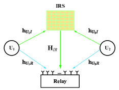
Figure 1: Diagram block for TWRN assisted by IRS.

User1 and User2 transmit their symbols to the relay simultaneously, and the receive signal at relay can be written as

$$\mathbf{y} =\sqrt{{P}_{{U}_{1}}}(\mathbf{H}_{IR}\bm{\Theta}\mathbf{h}_{{U}_{1}I}+\mathbf{h}_{{U}_{1}R})x_{{U}_{1}}$$

$$\quad+\sqrt{P_{{U}_{2}}}(\mathbf{H}_{IR}\bm{\Theta}\mathbf{h}_{{U}_{2}I}+\mathbf{h}_{{U}_{2}R})x_{{U}_{2}}+\mathbf{w}$$ (1)

where $\mathbf{y}\in\mathbb{C}^{K\times 1}$ denotes the received signal vector, $x_{{U}_{1}}$ and $x_{{U}_{2}}$ denote the transmitted symbol from user1 and user2, respectively, $\mathbf{w}\in\mathbb{C}^{K\times 1}$ denotes the receive additive white Gaussian noise with $\mathbf{w}\thicksim\mathcal{CN}(0,{\sigma}^{2}I)$, and the diagonal matrix $\bm{\Theta}$ is the phase matrix of IRS defined as

$$\bm{\Theta}=\text{diag}({\alpha}_{m}e^{-j{\vartheta}_{m}})=\text{diag}({\theta}_{m}),m=1,2,\ldots,M$$ (2)

where ${\alpha}_{m}\in(0,1]$ and ${\vartheta}_{m}\in[0,2\pi]$ ,$m=1,\ldots,M$ stand for the amplitude value and phase shift value of the $m$-th reflection elements, respectively. For simplicity, all of the amplitude values ${\alpha}_{m}$ are set to 1. In (II), the channel product $\bm{\Theta}\mathbf{h}_{SI}$ can be rewritten as follows

$$\bm{\Theta}\mathbf{h}_{{U}_{1}I} =[{\theta}_{1}h_{{U}_{1}I}(1),{\theta}_{2}h_{{U}_{1}I}(2),\ldots,{\theta}_{M}h_{{U}_{1}I}(M)]^{T}$$

$$=\mathbf{H}_{{U}_{1}I}\mathbf{\bm{\theta}}$$ (3)

where $\mathbf{H}_{{U}_{1}I}=\text{diag}(\mathbf{h}_{{U}_{1}I})$ and $\bm{\theta}\triangleq[{\theta}_{1},{\theta}_{2},\ldots,{\theta}_{M}]^{T}=[{\alpha}_{1}e^{-j{\vartheta}_{1}},{\alpha}_{2}e^{-j{\vartheta}_{2}},\ldots,{\alpha}_{M}e^{-j{\vartheta}_{M}}]^{T}$. Similarly, we can get $\bm{\Theta}\mathbf{h}_{{U}_{2}I}=\mathbf{H}_{{U}_{2}I}\mathbf{\bm{\theta}}$ where $\mathbf{H}_{{U}_{2}I}=\text{diag}(\mathbf{h}_{{U}_{2}I})$. By denoting the cascading channels as $\mathbf{H}_{{U}_{1}IR}=\mathbf{H}_{IR}\mathbf{H}_{{U}_{1}I}\in\mathbb{C}^{K\times M}$ and $\mathbf{H}_{{U}_{2}IR}=\mathbf{H}_{IR}\mathbf{H}_{{U}_{2}I}\in\mathbb{C}^{K\times M}$, the received signal (II) can be rewritten as

$$\mathbf{y} =\sqrt{P_{{U}_{1}}}(\mathbf{H}_{{U}_{1}IR}\bm{\theta}+\mathbf{h}_{{U}_{1}R})x_{{U}_{1}}$$

$$\quad+\sqrt{P_{{U}_{2}}}(\mathbf{H}_{{{U}_{2}}IR}\bm{\theta}+\mathbf{h}_{{{U}_{2}}R})x_{{U}_{2}}+\mathbf{w}.$$ (4)

III Proposed IRS channel estimator, pilot pattern and performance loss analysis

In this section, the LS channel estimator is proposed. Then, the optimal pilot pattern and phase shift training matrix are derived. Furthermore, in the scenario with a finite-phase-shifter IRS, the MSE performance loss factor is derived and analyzed due to the effect of quantization error.

III-A Proposed LS channel estimator

Fig. 2 shows the proposed pilot pattern. Here, user1 and user2 firstly send their pilot sequences $\mathbf{x}_{{U}_{1}}=[x_{{U}_{1}}(1),...,x_{{U}_{1}}(N_{P})]^{T}$ and $\mathbf{x}_{{U}_{2}}=[x_{{U}_{2}}(1),...,x_{{U}_{2}}(N_{P})]^{T}$ of $N_{P}$ symbols. Each symbol in the pilot sequence is related to a different IRS phase configuration $\bm{\theta}_{i}$, where $i=1,2,\ldots,N_{P}$. For user1 and user2, they transmit four continuous pilot sequences. Four sequences of the former are identical while the latter changes those sequence signs alternatively. Phase shift matrix $\mathbf{Q}$ change its signs in the latter two sequences.

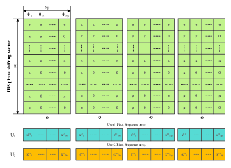
Figure 2: Proposed pilot pattern.

In the first pilot sequence period, the received signal can be expressed as

$$\mathbf{Y}_{1}=[\mathbf{y}_{1},\mathbf{y}_{2},\ldots,\mathbf{y}_{N_{P}}]=\sqrt{P_{{U}_{1}}}\mathbf{H}_{{U}_{1}IR}\mathbf{Q}\mathbf{X}_{{U}_{1}}+\sqrt{P_{{U}_{1}}}$$

$$\mathbf{h}_{{U}_{1}R}\mathbf{x}^{T}_{{U}_{1}}+\sqrt{P_{{U}_{2}}}\mathbf{H}_{{U}_{2}IR}\mathbf{Q}\mathbf{X}_{{U}_{2}}+\sqrt{P_{{U}_{2}}}\mathbf{h}_{{U}_{2}R}\mathbf{x}^{T}_{{U}_{2}}+\mathbf{W}_{1}$$ (5)

where $\mathbf{Q}=[\bm{\theta}_{1},\bm{\theta}_{2},\ldots,\bm{\theta}_{Np}]$, $\mathbf{X}_{{U}_{1}}=\text{diag}(\mathbf{x}_{{U}_{1}})$, and $\mathbf{X}_{{U}_{2}}=\text{diag}(\mathbf{x}_{{U}_{2}})$. Similarly, we have three receive signal matrices corresponding to the last three pilot sequences as follows

$$\mathbf{Y}_{2} =\sqrt{P_{{U}_{1}}}\mathbf{H}_{{U}_{1}IR}\mathbf{Q}\mathbf{X}_{{U}_{1}}+\sqrt{P_{{U}_{1}}}\mathbf{h}_{{U}_{1}R}\mathbf{x}^{T}_{{U}_{1}}$$

$$\quad-\sqrt{P_{{U}_{2}}}\mathbf{H}_{{U}_{2}IR}\mathbf{Q}\mathbf{X}_{{U}_{2}}-\sqrt{P_{{U}_{2}}}\mathbf{h}_{{U}_{2}R}\mathbf{x}^{T}_{{{U}_{1}}}+\mathbf{W}_{2},$$ (6)

$$\mathbf{Y}_{3} =-\sqrt{P_{{U}_{1}}}\mathbf{H}_{{U}_{1}IR}\mathbf{Q}\mathbf{X}_{{U}_{1}}+\sqrt{P_{{U}_{1}}}\mathbf{h}_{{U}_{1}R}\mathbf{x}^{T}_{{U}_{1}}$$

$$\quad-\sqrt{P_{{U}_{2}}}\mathbf{H}_{{U}_{2}IR}\mathbf{Q}\mathbf{X}_{{U}_{2}}+\sqrt{P_{{U}_{2}}}\mathbf{h}_{{U}_{2}R}\mathbf{x}^{T}_{{{U}_{1}}}+\mathbf{W}_{3},$$ (7)

and

$$\mathbf{Y}_{4} =-\sqrt{P_{{U}_{1}}}\mathbf{H}_{{U}_{1}IR}\mathbf{Q}\mathbf{X}_{{U}_{1}}+\sqrt{P_{S}}\mathbf{h}_{SR}\mathbf{x}^{T}_{S,P}$$

$$\quad+\sqrt{P_{{U}_{2}}}\mathbf{H}_{{U}_{2}IR}\mathbf{Q}\mathbf{X}_{{U}_{2}}-\sqrt{P_{{U}_{2}}}\mathbf{h}_{{U}_{2}R}\mathbf{x}^{T}_{{{U}_{1}}}+\mathbf{W}_{4}.$$ (8)

Observing the above four equations, due to their symmetric property, we have readily obtained the following four individual cascading and direct channels equations

$$\tilde{\mathbf{Y}}_{1}=\mathbf{Y}_{1}+\mathbf{Y}_{2} +\mathbf{Y}_{3}+\mathbf{Y}_{4}=4\sqrt{P_{{U}_{1}}}\mathbf{h}_{{U}_{1}R}\mathbf{x}^{T}_{{U}_{1}}$$

$$\quad+\mathbf{W}_{1}+\mathbf{W}_{2}+\mathbf{W}_{3}+\mathbf{W}_{4}$$ (9)

$$\tilde{\mathbf{Y}}_{2}=\mathbf{Y}_{1}-\mathbf{Y}_{2} +\mathbf{Y}_{3}-\mathbf{Y}_{4}=4\sqrt{P_{{U}_{2}}}\mathbf{h}_{{U}_{2}R}\mathbf{x}^{T}_{{U}_{2}}$$

$$\quad+\mathbf{W}_{1}-\mathbf{W}_{2}+\mathbf{W}_{3}-\mathbf{W}_{4}$$ (10)

$$\tilde{\mathbf{Y}}_{3}=\mathbf{Y}_{1}+\mathbf{Y}_{2} -\mathbf{Y}_{3}-\mathbf{Y}_{4}=4\sqrt{P_{{U}_{1}}}\mathbf{H}_{{U}_{1}IR}\mathbf{Q}\mathbf{X}_{{U}_{1}}$$

$$\quad+\mathbf{W}_{1}+\mathbf{W}_{2}-\mathbf{W}_{3}-\mathbf{W}_{4}$$ (11)

$$\tilde{\mathbf{Y}}_{4}=\mathbf{Y}_{1}-\mathbf{Y}_{2} -\mathbf{Y}_{3}+\mathbf{Y}_{4}=4\sqrt{P_{{U}_{2}}}\mathbf{H}_{{U}_{2}IR}\mathbf{Q}\mathbf{X}_{{U}_{2}}$$

$$\quad+\mathbf{W}_{1}-\mathbf{W}_{2}-\mathbf{W}_{3}+\mathbf{W}_{4}$$ (12)

where the number of columns of matrix $\mathbf{Q}$ is chosen to be greater than or equal to the number of its rows in order to ensure that $\mathbf{Q}$ is invertible, i.e. $N_{P}\geq M$. To reduce the estimation overheads, it is assumed that $N_{P}=M$. Multiplying (III-A) by $\mathbf{x}^{*}_{{U}_{1}}$ from the right gives

$$\tilde{\mathbf{Y}}_{1}\mathbf{x}^{*}_{{U}_{1}P} =4\sqrt{P_{{U}_{1}}}\mathbf{h}_{{U}_{1}R}\mathbf{x}^{T}_{{U}_{1},P}\mathbf{x}^{*}_{{U}_{1}}$$

$$\quad+(\mathbf{W}_{1}+\mathbf{W}_{2}+\mathbf{W}_{3}+\mathbf{W}_{4})\mathbf{x}^{*}_{{U}_{1}}$$ (13)

which yields the LS estimation of $\mathbf{h}_{{U}_{1}R}$.

$$\hat{\mathbf{h}}_{{U}_{1}R}=\tfrac{\tilde{\mathbf{Y}}_{1}\mathbf{x}^{*}_{{U}_{1}}}{4\sqrt{P_{{U}_{1}}}\mathbf{x}^{T}_{{U}_{1}}\mathbf{x}^{*}_{{U}_{1}}}.$$ (14)

Similarly,

$$\hat{\mathbf{h}}_{{U}_{2}R}=\tfrac{\tilde{\mathbf{Y}}_{2}\mathbf{x}^{*}_{{U}_{2}}}{4\sqrt{P_{{U}_{1}}}\mathbf{x}^{T}_{{U}_{2}}\mathbf{x}^{*}_{{U}_{2}}}.$$ (15)

Now, letting us turn to the cascading channels, performing vec operation on two sides of Eq.(III-A) forms

$$\text{vec}(\tilde{\mathbf{Y}}_{3}) =4\sqrt{P_{{U}_{1}}}(\overbrace{(\mathbf{Q}\mathbf{X}_{{U}_{1}})^{T}\otimes\mathbf{I}_{K}}^{\mathbf{A}_{{U}_{1}}})\text{vec}(\mathbf{H}_{{U}_{1}IR})$$

$$\quad+\text{vec}(\mathbf{W}_{1}+\mathbf{W}_{2}-\mathbf{W}_{3}-\mathbf{W}_{4})$$ (16)

which gives the LS estimator of $\mathbf{H}_{{U}_{1}IR}$ as follows

$$\text{vec}(\hat{\mathbf{H}}_{{U}_{1}IR})=\tfrac{\mathbf{A}_{{U}_{1}}^{-1}\text{vec}(\tilde{\mathbf{Y}}_{3})}{4\sqrt{P_{{U}_{1}}}}.$$ (17)

Similarly, we have

$$\text{vec}(\hat{\mathbf{H}}_{{U}_{2}IR})=\tfrac{\mathbf{A}_{{U}_{2}}^{-1}\text{vec}(\tilde{\mathbf{Y}}_{4})}{4\sqrt{P_{{U}_{2}}}}.$$ (18)

Given $\mathbb{E}\{\mathbf{x}^{T}_{{U}_{1}}\mathbf{x}^{*}_{{U}_{1}}\}=M$, the MSE of estimating $\mathbf{h}_{{U}_{1}R}$ is

$$\epsilon_{1} =\tfrac{1}{4M}\mathbb{E}\{\|\hat{\mathbf{h}}_{{U}_{1}R}-\mathbf{h}_{{U}_{1}R}\|^{2}_{F}\}$$

$$=\tfrac{1}{4M}\mathbb{E}\{\|\tfrac{\tilde{\mathbf{Y}}_{1}\mathbf{x}^{*}_{{U}_{1}}}{4\sqrt{P_{S}}\mathbf{x}^{T}_{{U}_{1}}\mathbf{x}^{*}_{{U}_{1}}}-\mathbf{h}_{{U}_{1}R}\|^{2}_{F}\}$$

$$=\tfrac{1}{4M}\mathbb{E}\{\|\tfrac{(4\sqrt{P_{{U}_{1}}}\mathbf{h}_{SR}\mathbf{x}^{T}_{{U}_{1}}+\mathbf{W}_{1}+\mathbf{W}_{2}+\mathbf{W}_{3}+\mathbf{W}_{4})\mathbf{x}^{*}_{{U}_{1}}}{4\sqrt{P_{{U}_{1}}}\mathbf{x}^{T}_{{U}_{1}}\mathbf{x}^{*}_{{U}_{1}}}-\mathbf{h}_{{U}_{1}R}\|^{2}_{F}\}$$

$$=\tfrac{1}{4M}\mathbb{E}\{\|\tfrac{(\mathbf{W}_{1}+\mathbf{W}_{2}+\mathbf{W}_{3}+\mathbf{W}_{4})\mathbf{x}^{*}_{{U}_{1}}}{4\sqrt{P_{{U}_{1}}}\mathbf{x}^{T}_{{U}_{1}}\mathbf{x}^{*}_{{U}_{1}}}\|^{2}_{F}\}$$

$$=\tfrac{1}{64P_{{U}_{1}}M^{3}}\mathbb{E}\{\|(\mathbf{W}_{1}+\mathbf{W}_{2}+\mathbf{W}_{3}+\mathbf{W}_{4})\mathbf{x}^{*}_{{U}_{1}}\|^{2}_{F}\}$$

$$=\tfrac{{\sigma}^{2}}{16P_{{U}_{1}}M^{2}}$$ (19)

Similarly, we have the remaining MSEs

$$\epsilon_{2}=\tfrac{{\sigma}^{2}}{16P_{{U}_{2}}M^{2}},$$ (20)

$$\epsilon_{3}=\tfrac{1}{4M}\mathbf{E}\{\|\text{vec}(\hat{\mathbf{H}}_{{U}_{1}IR})-\text{vec}(\mathbf{H}_{{U}_{1}IR})\|^{2}_{F}\}$$

$$=\tfrac{1}{4M}\mathbf{E}\{\|\tfrac{\mathbf{A}_{{U}_{1}}^{-1}\text{vec}(\tilde{\mathbf{Y}}_{3})}{4\sqrt{P_{{U}_{1}}}}-\text{vec}(\mathbf{H}_{{U}_{1}IR})\|^{2}_{F}\}$$

$$=\tfrac{1}{4M}\mathbf{E}\{\|\tfrac{\mathbf{A}_{{U}_{1}}^{-1}(4\sqrt{P_{{U}_{1}}}\mathbf{A}_{{U}_{1}}\text{vec}(\mathbf{H}_{{U}_{1}IR})+\text{vec}(\mathbf{W}_{1}+\mathbf{W}_{2}-\mathbf{W}_{3}-\mathbf{W}_{4}))}{4\sqrt{P_{{U}_{1}}}}$$

$$-\text{vec}(\mathbf{H}_{{U}_{1}IR})\|^{2}_{F}\}=\tfrac{1}{4M}\mathbf{E}\{\|\tfrac{\mathbf{A}_{{U}_{1}}^{-1}\text{vec}(\mathbf{W}_{1}+\mathbf{W}_{2}-\mathbf{W}_{3}-\mathbf{W}_{4})}{4\sqrt{P_{{U}_{1}}}}\|^{2}_{F}\}$$

$$=\tfrac{4{\sigma}^{2}\text{tr}((\mathbf{A}_{{U}_{1}}^{-1})^{H}\mathbf{A}_{{U}_{1}}^{-1})}{64P_{{U}_{1}}M}=\tfrac{{\sigma}^{2}\text{tr}((\mathbf{A}_{{U}_{1}}^{-1})^{H}\mathbf{A}_{{U}_{1}}^{-1})}{16P_{{U}_{1}}M},$$ (21)

and

$$\epsilon_{4}=\tfrac{{\sigma}^{2}\text{tr}((\mathbf{A}_{{U}_{2}}^{-1})^{H}\mathbf{A}_{{U}_{2}}^{-1})}{16P_{{U}_{2}}M},$$ (22)

which directly yields the Sum-MSE as follows

$$\epsilon=\epsilon_{1}+\epsilon_{2}+\epsilon_{3}+\epsilon_{4}.$$ (23)

III-B Pilot optimization of minimizing Sum-MSE

Since from Eq. (III-A),

$$\mathbf{A}_{{U}_{1}}^{-1}=\overbrace{(\mathbf{Q}^{T})^{-1}}^{\mathbf{B}}\mathbf{X}^{-1}_{{U}_{1}}\otimes\mathbf{I}_{K},$$ (24)

we have

$$\text{tr}\{(\mathbf{A}_{{U}_{1}}^{-1})^{H}\mathbf{A}_{{U}_{1}}^{-1}\}=\text{tr}\{((\mathbf{X}^{-1}_{{U}_{1}})^{H}\mathbf{B}^{H})\otimes\mathbf{I}_{K})(\mathbf{B}\mathbf{X}^{-1}_{{U}_{1}}\otimes\mathbf{I}_{K})\}$$

$$=\text{tr}\{(\mathbf{X}^{-1}_{{U}_{1}})^{H}\mathbf{B}^{H}\mathbf{B}\mathbf{X}^{-1}_{{U}_{1}}\otimes\mathbf{I}_{K})\}$$

$$=K\text{tr}\{(\mathbf{X}^{-1}_{{U}_{1}})^{H}\mathbf{B}^{H}\mathbf{B}\mathbf{X}^{-1}_{{U}_{1}}\}=K\text{tr}\{(\mathbf{X}_{{U}_{1}}^{H}\mathbf{X}_{{U}_{1}})^{-1}\mathbf{B}^{H}\mathbf{B}\}$$

$$=K\text{tr}\{(\mathbf{X}_{{U}_{1}}^{H}\mathbf{X}_{{U}_{1}})^{-1}(\mathbf{Q}^{T}\mathbf{Q}^{*})^{-1}\}$$ (25)

Minimizing Eq. (III-B) can be decomposed into the following two sub-problems

$$\text{(P1.1)}:\quad \underset{\mathbf{Q}}{\min}\ \text{tr}\{(\mathbf{Q}^{T}\mathbf{Q}^{*})^{-1}\}$$

$$\text{ s.t. }|\theta_{t}(m)|=1,t=1,2,\ldots,M,$$

$$\quad\quad\quad\quad\quad\quad\quad m=1,2,\ldots,M,$$ (26)

and

$$\text{(P1.2)}:\quad \min K(\text{tr}((\mathbf{X}^{-1}_{{U}_{1}})^{H}\mathbf{X}^{-1}_{{U}_{1}}))$$

$$\text{ s.t. }\tfrac{\text{tr}\{\mathbf{X}_{{U}_{1}}\mathbf{X}^{H}_{{U}_{1}}\}}{N_{P}}=1$$ (27)

According to [12, 13, 17], we have $\|X_{{U}_{1}}(i)\|^{2}=\|X_{{U}_{2}}(i)\|^{2}=1,\forall i\in\{1,2,\ldots,N_{P}\}$ and $\mathbf{Q}^{H}\mathbf{Q}=M\mathbf{I}_{M}$. Finally, the minimum of Sum-MSE $\epsilon$ can be given by

$$\epsilon_{min}=\tfrac{K\sigma^{2}}{16P_{{U}_{1}}M}+\tfrac{K\sigma^{2}}{16P_{{U}_{2}}M}+\tfrac{{\sigma}^{2}}{16P_{{U}_{1}}M^{2}}+\tfrac{{\sigma}^{2}}{16P_{{U}_{2}}M^{2}}$$ (28)

III-C Performance loss analysis

To satisfy $\text{tr}\{(\mathbf{Q}^{T}\mathbf{Q}^{*})^{-1}\}=1$ and the constant modulus constraint, the training matrix $\mathbf{Q}$ is usually chosen to be a DFT matrix in existing research works in [12, 13]. The DFT matrix is optimal for an IRS with high-resolution or infinite-phase shifters. But for an IRS with low-resolution phase shifters, we propose a Hadamard matrix to replace a DFT matrix. The $N$-points DFT matrix is denoted by $\mathbf{Q}_{DFT}$, which is given by

$$[\mathbf{Q}_{DFT}]_{m,n}=e^{-j\tfrac{2\pi(m-1)(n-1)}{M}},1\leq m,n\leq N.$$ (29)

What’s more, Hadamard matrix is an orthogonal matrix whose entry is given by 1 or -1. An example of $4\times 4$ Hadamard matrix is as follows

$$\mathbf{Q}_{Hadamard}=\left[\begin{array}[]{cccc}+1&+1&+1&+1\\ +1&-1&+1&-1\\ +1&+1&-1&-1\\ +1&-1&-1&+1\\ \end{array}\right].$$ (34)

Actually, a Hadamard matrix only contains 1-bit phase shifter to achieve an optimal performance. A DFT matrix requires at least ${\log}_{2}M$-bit phase shifter for each reflection element of the IRS. As $M$ tends to large-scale, this will lead to a high circuit cost.

Assuming IRS adopts phase shifters with $L$ being the number of discrete phases per phase shifter, each reflection element’s phase in $\mathbf{Q}$ takes its nearest value $\tilde{\vartheta}$ from the following set

$$\tilde{\vartheta}\in\bm{\Phi}=\big{\{}\tfrac{\pi}{L},\tfrac{3\pi}{L},\ldots,\tfrac{(2L-1)\pi}{L}\big{\}}$$ (35)

which forms the quantized version $\tilde{\mathbf{Q}}$ of matrix $\mathbf{Q}$. Here, phase quantization noise is assumed to be uniformly distributed. Now, let us define the performance loss factor as follows

$$\beta=\tfrac{\text{tr}\{(\tilde{\mathbf{Q}}^{T}\tilde{\mathbf{Q}}^{*})^{-1}\}}{\text{tr}\{(\mathbf{Q}^{T}\mathbf{Q}^{*})^{-1}\}}$$ (36)

Note that $\text{tr}\{(\mathbf{Q}^{T}\mathbf{Q}^{*})^{-1}\}=1$. (36) can be simplified as

$$\beta=\text{tr}\{(\tilde{\mathbf{Q}}^{T}\tilde{\mathbf{Q}}^{*})^{-1}\}$$ (37)

When the number of quantization bits is large, $\beta$ can be approximated as

$$\beta\approx 3-2\text{sinc}(\tfrac{\pi}{L})$$ (38)

Proof: See Appendix A.

IV Simulation results

In this section, we perform some numerical simulation to evaluate the performance of IRS-aided TWRN system. System parameters are set as follows: $M=128$, $K=16$. It is assumed that User1, User2, Relay, and IRS are in the same plane and the coordinates of User1, User2, Relay, and IRS are (0,0), (100m,0), (0,50m), and (10m,50m), respectively. The path loss exponents of the $\text{User1/User2}\rightarrow\text{R}$, $\text{User1/User2}\rightarrow\text{IRS}$ and $\text{IRS}\rightarrow\text{R}$ are set as 3.5, 2.4, and 2.2, respectively. The path loss at the reference distance of 1 m is chosen as 30 dB. The variance of the noise $\sigma^{2}$ is -80 dBm. The transmitting powers of User1 and User2 are the same, i.e. $P_{{U}_{1}}=P_{{U}_{2}}$. The definition of SNR is $P_{{U}_{1}}/\sigma^{2}$.

Fig. 3 shows the MSE versus SNR with $M=128$ with IRS being random phase matrix (RPM) as a performance benchmark. It is seen that the Hadamard matrix and DFT matrix performs much better than RPM, and achieve the same performance for all values of SNRs because of $\text{tr}\{\mathbf{Q}^{*}\mathbf{Q}^{T}\}=M\mathbf{I}_{M}$. Compared to other channel estimation methods, the sum-MSE of the proposed scheme is smaller than those in [12, 15] due to a higher pilot training overhead in our scheme.

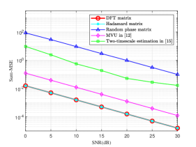
Figure 3: Sum-MSE versus different SNRs with $M$=128.

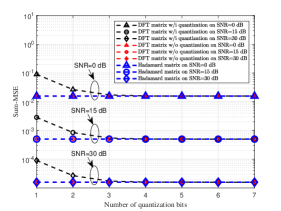
Figure 4: Sum-MSE versus number of quantization bit with different SNRs, and $M$=128.

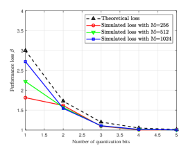
Figure 5: Theoretical and simulated performance loss versus number of quantization bits with different $M$.

Fig. 4 shows the Sum-MSE versus the number of phase quantization bits for three typical SNRs 0 dB, 15 dB, and 30 dB and $M=128$. It can be seen that as the number of quantization bits increases, the corresponding Sum-MSE approaches the Sum-MSE of infinite precision phase shifter. the performance loss trend is independent of the values of SNR. Particularly, the channel estimation performance with 3$\sim$4 bit phase shifters is very close to that of the infinite-bit case. This means 3$\sim$4 bits are sufficient for TWRN aided by IRS with finite-bit phase shifters to achieve an omitted performance loss. It is clear that the Hadamard matrix achieves the same Sum-MSE performance as the DFT matrix with infinite bits as the number of quantization bits varies from 1 to 7.

Fig. 5 illustrates the derived theoretical performance loss factor in (46) versus the number of phase quantization bits with numerical simulated losses for different $M$ as performance references. The trend in Fig. 5 is consistent with that in Fig. 4. As the number of elements of IRS goes to large-scale, the simulated loss factor become closer to the theoretical expression derived in (46). Thus, this theoretical expression can be approximately used to make an analysis of performance loss due to the effect of the number of phase quantization bits.

V Conclusion

In this paper , we have investigated channel estimation, pilot design and performance loss analysis of an TWRN aided by IRS with finite-bit phase shifters. To estimate both the direct and cascaded channels, an excellent pilot pattern was designed, and the LS channel estimator was presented. Additionally, the MSE performance loss factor was defined, derived and analyzed. From theoretical analysis and simulation results, if the phase matrix of IRS is chosen to be the Hadamard matrix instead of conventional DFT matrix, then it can achieve an optimal MSE performance in the case of 1-bit phase shifters of IRS. However, the DFT matrix uses 3$\sim$4-bit phase shifter of IRS also to achieve the optimal performance.

Appendix A Proof of performance loss

Proof: The quantization error can be defined as $\Delta\mathbf{Q}=\mathbf{Q}-\tilde{\mathbf{Q}}$.

$$\text{tr}\{(\tilde{\mathbf{Q}}^{T}\tilde{\mathbf{Q}}^{*})^{-1}\}=\text{tr}\{\big{(}(\mathbf{Q}-\Delta\mathbf{Q})^{T}(\mathbf{Q}-\Delta\mathbf{Q})^{*}\big{)}^{-1}\}$$

$$=\text{tr}\{\big{(}(\mathbf{Q}^{T}-\Delta\mathbf{Q}^{T})(\mathbf{Q}^{*}-\Delta\mathbf{Q}^{*})\big{)}^{-1}\}=\text{tr}\{$$

$$\big{(}\mathbf{Q}^{T}\mathbf{Q}^{*}-\mathbf{Q}^{T}\Delta\mathbf{Q}^{*}-\Delta\mathbf{Q}^{T}\mathbf{Q}^{*}+\Delta\mathbf{Q}^{T}\Delta\mathbf{Q}^{*}\big{)}^{-1}\}$$ (39)

Note that $\mathbf{Q}^{*}\mathbf{Q}^{T}=M\mathbf{I}_{M}$. Obliviously, $\text{tr}\{(\mathbf{Q}^{T}\mathbf{Q}^{*})^{-1}\}=1$. Considering that the quantization error at high quantization accuracy becomes extremely small, the inverse of Gram matrix $\tilde{\mathbf{Q}}^{T}\tilde{\mathbf{Q}^{*}}$ has the following linear approximation

$$(\tilde{\mathbf{Q}}^{T}\tilde{\mathbf{Q}}^{*})^{-1}\approx\big{(}M\mathbf{I}_{M}-\underbrace{(\mathbf{Q}^{T}\Delta\mathbf{Q}^{*}+\Delta\mathbf{Q}^{T}\mathbf{Q}^{*})}_{\Delta\mathbf{I}}\big{)}^{-1}$$

$$=(M(\mathbf{I}_{M}-\tfrac{1}{M}\Delta\mathbf{I}))^{-1}=\tfrac{1}{M}(\mathbf{I}_{M}+\tfrac{1}{M}\Delta\mathbf{I})$$ (40)

which yields

$$\text{tr}\{(\tilde{\mathbf{Q}}^{T}\tilde{\mathbf{Q}}^{*})^{-1}\}=1+\tfrac{1}{M^{2}}\text{tr}\{\Delta\mathbf{I}\}$$ (41)

Now, we simplify the second term of the right side of the above equation as follows

$$\tfrac{1}{M^{2}}\text{tr}\{\Delta\mathbf{I}\}=\tfrac{2}{M^{2}}\text{tr}\{\mathbf{Q}^{T}\Delta\mathbf{Q}^{*}+\Delta\mathbf{Q}^{T}\mathbf{Q}^{*}\}=2\text{tr}\{\mathbf{Q}^{T}\Delta\mathbf{Q}^{*}\}$$

$$=\tfrac{2}{M^{2}}\text{tr}\{\mathbf{Q}^{T}(\mathbf{Q}-\mathbf{Q}\odot\Delta\mathbf{Q})^{*}\}$$

$$=\tfrac{1}{M^{2}}\sum_{i=1}^{M}\sum_{m=1}^{M}\mathbf{Q}^{*}_{(i,m)}(\mathbf{Q}-\mathbf{Q}\odot\Delta\mathbf{Q})^{T}_{(i,m)}=\tfrac{2}{M^{2}}\sum_{i=1}^{M}\sum_{m=1}^{M}$$

$$e^{j\vartheta_{im}}e^{-j\vartheta_{im}}(1-e^{-j\Delta\vartheta_{im}})=\tfrac{2}{M^{2}}\sum_{i=1}^{M}\sum_{m=1}^{M}(1-e^{-j\Delta\vartheta_{im}})$$ (42)

Using the above equation and considering that the phase error is assumed to be uniform distribution over the interval [$-\frac{\pi}{L},\frac{\pi}{L}$], we have

$$\tfrac{1}{M^{2}}\text{tr}(\Delta\mathbf{I}) =2\int^{\tfrac{\pi}{L}}_{-\tfrac{\pi}{L}}p(\Delta\vartheta_{im})(1-e^{-j\Delta\vartheta_{im}})d(\Delta\vartheta_{im})$$ (43)

where

$$p(\Delta\vartheta_{im})=\tfrac{L}{2\pi}.$$ (44)

Finally, we have

$$2\int^{\tfrac{\pi}{L}}_{-\tfrac{\pi}{L}}\tfrac{L}{2\pi}(1-e^{-j\Delta\vartheta_{im}})d(\vartheta_{im})=2-2\text{sinc}(\frac{\pi}{L}),$$ (45)

Substituting (45) in (43) and then (43) in (41) directly gives

$$\text{tr}\{(\tilde{\mathbf{Q}}^{T}\tilde{\mathbf{Q}}^{*})^{-1}\}\approx 3-2\text{sinc}(\tfrac{\pi}{L}).$$ (46)

This completes the proof of performance loss factor.

References

• [1] Y. Zou, J. Zhu, and X. Jiang, “Joint power splitting and relay selection in energy-harvesting communications for IoT networks,” IEEE Internet of Things J., vol. 7, no. 1, pp. 584–597, Oct. 2020.
• [2] Q. Wu and R. Zhang, “Towards smart and reconfigurable environment: Intelligent reflecting surface aided wireless network,” IEEE Commun. Mag., vol. 58, no. 1, pp. 106–112, Jan. 2020.
• [3] X. Chen, D. W. K. Ng, W. Yu, E. G. Larsson, N. Al-Dhahir, and R. Schober, “Massive access for 5G and beyond,” IEEE J. Sel. Areas Commun., vol. 39, no. 3, pp. 615–637, Sep. 2021.
• [4] H.-M. Wang, J. Bai, and L. Dong, “Intelligent reflecting surfaces assisted secure transmission without eavesdropper’s CSI,” IEEE Signal Process. Lett., vol. 27, pp. 1300–1304, Jul. 2020.
• [5] F. Shu, Y. Teng, J. Li, M. Huang, W. Shi, J. Li, Y. Wu, and J. Wang, “Enhanced secrecy rate maximization for directional modulation networks via IRS,” IEEE Trans. Commun., pp. 1–1, Sep. 2021.
• [6] X. Cheng, Y. Lin, W. Shi, J. Li, C. Pan, F. Shu, Y. Wu, and J. Wang, “Joint optimization for RIS-assisted wireless communications: From physical and electromagnetic perspectives,” IEEE Trans. Commun., pp. 1–1, Oct. 2021.
• [7] W. Shi, X. Zhou, L. Jia, Y. Wu, F. Shu, and J. Wang, “Enhanced secure wireless information and power transfer via intelligent reflecting surface,” IEEE Commun. Lett., vol. 25, no. 4, pp. 1084–1088, Dec. 2020.
• [8] X. Zhou, S. Yan, Q. Wu, F. Shu, and D. W. K. Ng, “Intelligent reflecting surface (IRS)-aided covert wireless communications with delay constraint,” IEEE Trans. Wireless Commun., pp. 1–1, Jul. 2021.
• [9] X. Wang, F. Shu, W. Shi, X. Liang, R. Dong, J. Li, and J. Wang, “Beamforming design for IRS-aided decode-and-forward relay wireless network,” 2021. [Online]. Available: https://arxiv.org/abs/2109.10657
• [10] Z. Abdullah, G. Chen, S. Lambotharan, and J. A. Chambers, “A hybrid relay and intelligent reflecting surface network and its ergodic performance analysis,” IEEE Wireless Commun. Lett., vol. 9, no. 10, pp. 1653–1657, Oct. 2020.
• [11] Y. Zhou, J. Wang, and M. Sawahashi, “Downlink transmission of broadband OFCDM systems-part II: effect of Doppler shift,” IEEE Trans. Commun., vol. 54, no. 6, pp. 1097–1108, Jun. 2006.
• [12] T. L. Jensen and E. De Carvalho, “An optimal channel estimation scheme for intelligent reflecting surfaces based on a minimum variance unbiased estimator,” in ICASSP 2020 - 2020 IEEE International Conference on Acoustics, Speech and Signal Processing (ICASSP), May. 2020, pp. 5000–5004.
• [13] B. Zheng, C. You, and R. Zhang, “Intelligent reflecting surface assisted multi-user OFDMA: Channel estimation and training design,” IEEE Trans. Wireless Commun., vol. 19, no. 12, pp. 8315–8329, Sep. 2020.
• [14] X. Guan, Q. Wu, and R. Zhang, “Anchor-assisted intelligent reflecting surface channel estimation for multiuser communications,” in GLOBECOM 2020 - 2020 IEEE Global Communications Conference, Dec. 2020, pp. 1–6.
• [15] C. Hu, L. Dai, S. Han, and X. Wang, “Two-timescale channel estimation for reconfigurable intelligent surface aided wireless communications,” IEEE Trans. Commun., vol. 69, no. 11, pp. 7736–7747, Nov. 2021.
• [16] C. You, B. Zheng, and R. Zhang, “Intelligent reflecting surface with discrete phase shifts: Channel estimation and passive beamforming,” in ICC 2020 - 2020 IEEE International Conference on Communications (ICC), 2020, pp. 1–6.
• [17] F. Shu, J. Wang, J. Li, R. Chen, and W. Chen, “Pilot optimization, channel estimation, and optimal detection for full-duplex OFDM systems with IQ imbalances,” IEEE Trans. Veh. Technol., vol. 66, no. 8, pp. 6993–7009, Feb. 2017.