Sayer: Using Implicit Feedback to Optimize System Policies

Abstract.

We observe that many system policies that make threshold decisions involving a resource (e.g., time, memory, cores) naturally reveal additional, or implicit feedback. For example, if a system waits $X$ min for an event to occur, then it automatically learns what would have happened if it waited $<X$ min, because time has a cumulative property. This feedback tells us about alternative decisions, and can be used to improve the system policy. However, leveraging implicit feedback is difficult because it tends to be one-sided or incomplete, and may depend on the outcome of the event. As a result, existing practices for using feedback, such as simply incorporating it into a data-driven model, suffer from bias.

We develop a methodology, called Sayer, that leverages implicit feedback to evaluate and train new system policies. Sayer builds on two ideas from reinforcement learning—randomized exploration and unbiased counterfactual
estimators—to leverage data collected by an existing policy to estimate the performance of new candidate policies, without actually deploying those policies. Sayer uses implicit exploration and implicit data augmentation to generate implicit feedback in an unbiased form, which is then used by an implicit counterfactual estimator to evaluate and train new policies. The key idea underlying these techniques is to assign implicit probabilities to decisions that are not actually taken but whose feedback can be inferred; these probabilities are carefully calculated to ensure statistical unbiasedness. We apply Sayer to two production scenarios in Azure, and show that it can evaluate arbitrary policies accurately, and train new policies that outperform the production policies.

1. Introduction

A system policy is any logic that makes decisions for a system, such as choosing a configuration, setting a timeout value, or deciding how to handle a request. System policies are pervasive in cloud infrastructure and can seriously impact the performance of a system. For this reason, developers are constantly trying to iterate on and improve them. Typically this is done by collecting feedback from the currently deployed policy and analyzing or processing it to generate new candidate policies. The more feedback that can be collected, the more insights that can be learned to improve the policy.

We observe that a large class of system policies naturally reveal additional feedback beyond the decision that is actually made. These policies make threshold decisions involving a resource such as time, memory, or cores. Since the resources are naturally cumulative, thresholding on one value often reveals feedback for other values as well. For example, consider a system policy that decides how long to wait for an unresponsive machine before rebooting it. If the policy waits $X$ min, then it automatically learns what would have happened if it waited $<$$X$ minutes, because time is cumulative. We call this kind of feedback implicit feedback.

Ideally, we would like to leverage implicit feedback to evaluate new candidate policies and ask: what would happen if we deployed this policy in production? This type of “what-if” question can be answered using counterfactual evaluation, a process that uses data collected from a deployed policy to estimate the performance of a candidate policy. If counterfactual evaluation can be done offline, it provides a powerful alternative to methods like A/B testing (which require live deployment of a policy), because it means that we can evaluate policies without ever deploying them (Horvitz and Thompson, 1952).

Unfortunately, implicit feedback is difficult to leverage because it typically appears in a biased form. For instance in the above example, feedback is only received for wait times $<$$X$, i.e., it is one-sided. In fact, the amount of feedback received may even depend on the outcome of an event: if the unresponsive machine recovers within $X$ min, then we actually get feedback for any wait time, because we know exactly when the machine recovered. Biased feedback is difficult to leverage for counterfactual evaluation because it generates more feedback for some actions than for others. For example, a policy that always waits $\leq$3 min will never generate feedback that can be used to evaluate a candidate policy that waits 4 min or more.

How do we leverage implicit feedback that is one-sided and outcome-dependent? We draw on ideas from statistics and reinforcement learning (RL) to provide a starting point. Specifically, we leverage: randomized exploration, which modifies a deployed policy to choose a random action some of the time, thereby increasing the coverage over all actions; and unbiased counterfactual estimators, which use exploration data collected from a policy to accurately estimate a candidate policy’s performance. The threshold decisions we study naturally satisfy certain independence assumptions (§3.1), allowing us to build on particularly efficient exploration algorithms and counterfactual estimators. Unfortunately, all of these techniques assume that a policy receives feedback only for the (single) action that it takes. In other words, they are unable to leverage implicit feedback.

We develop a methodology called Sayer that leverages implicit feedback to perform unbiased counterfactual evaluation and training of system policies. Sayer develops three techniques to harness the implicit feedback revealed by threshold decisions: (1) implicit exploration builds on existing exploration algorithms to maximize the amount of implicit feedback generated; (2) implicit data augmentation augments the logged data from a deployed policy to include implicit feedback; and (3) an implicit counterfactual estimator uses the augmented data to evaluate and train new policies in an unbiased manner. A key idea underlying Sayer is to assign implicit probabilities to decisions that are not actually taken but whose feedback can be inferred; these probabilities are carefully calculated to ensure statistical unbiasedness.

As a community, we have developed a variety of methods for counterfactual evaluation, ranging from offline methods like simulators and data-driven models, to online methods like A/B testing. However, as we discuss in §2.3, most of these approaches suffer from bias, and approaches that are unbiased are either too invasive (e.g., they require a live deployment) or are not data-efficient. None of these approaches leverage implicit feedback. In contrast, Sayer builds on techniques from RL to enable unbiased and data-efficient counterfactual evaluation.

Contributions.  Sayer makes the following contributions:

• We demonstrate the presence of implicit feedback in system policies that make threshold decisions (§2), and develop a framework for harnessing this feedback. Sayer provides a new unbiased counterfactual estimator for implicit feedback, supported by new implicit feedback-aware algorithms for exploration and data augmentation (§3).

• We develop an architecture for integrating Sayer into the lifecycle of existing system policies (§3.1), supporting their continuous optimization lifecycle (§3.3). This enables policies to continuously evolve.

• We apply Sayer to two production scenarios in Azure: (§4.2-§4.3): Azure-Health, a system that handles unresponsive machines, and Azure-Scale, a system that creates scalable sets of virtual machines.

2. Implicit Feedback

This section provides the necessary background for studying system policies that yield implicit feedback. We first show that threshold decisions naturally reveal additional, implicit feedback beyond the decision that is actually taken (§2.1). Leveraging this feedback to evaluate new policies is difficult, however, because it appears in a biased form (§2.2). A survey of existing approaches for policy evaluation (§2.3) shows that reinforcement learning (RL) provides a foundation for addressing this bias. However, no existing approach, including RL ones, can leverage implicit feedback, motivating the goals of Sayer (§2.4).

2.1. Implicit Feedback in Threshold Decisions

Many system policies make threshold decisions based on a resource such as time, memory, cores, etc.. These decisions choose a threshold value of the resource on which some behavior of the system is conditioned. Some real examples of threshold decisions made in the Azure cloud include:

• time: How long to wait for unresponsive machines before rebooting them (Azure-Health, §4.2).

• VMs: How many extra VMs to create in order to complete a set of VM creations faster (Azure-Scale, §4.3).

• cores: What level of CPU utilization triggers an elastic scaler to increase/decrease the number of replicas?

Decisions like these are pervasive in cloud infrastructure and can seriously impact the performance of a system. We study two of these decisions in this paper. As a running example we use Azure-Health, a system which monitors the health of physical machines in Azure’s datacenters, with the goal of minimizing downtime for customer VMs. If a machine becomes unresponsive, a system policy decides how long to wait for the machine to recover before rebooting it and reprovisioning its VMs, a process that may take $>$10 min. The policy chooses a wait time from $\{1,2,\ldots,10\}$ min (the longest wait time being comparable to the reboot cost).

In each of the above examples, the resource in question has a natural cumulative property. For example, if the Azure-Health policy waits $X$ min for an unresponsive machine, this automatically tells us what would have happened if it waited $<$$X$ min, because time is cumulative. Similarly, allocating $X$ extra VMs tells us what would have happened if we allocated fewer VMs, and scaling up at $X\%$ CPU utilization tell us about lower thresholds. Interestingly, feedback can also be revealed for thresholds greater than the chosen action. For example in Azure-Health, if we wait $X$ min for an unresponsive machine and it recovers within that time, then we actually get feedback for all other waiting times, since we know exactly when the machine recovers. In this case, the amount of feedback depends on the outcome of an event.

In all of the above examples, feedback is revealed for a decision that was not actually taken, but can be inferred from the decision that was taken. We call this implicit feedback.

2.2. The Bias Problem

Implicit feedback has the potential to accelerate improvements to system policies, because it allows developers to ask “what if” questions about alternative policy decisions. For example, an Azure-Health developer may ask: what if we waited longer for all unresponsive machines, or what if we waited less time for newer machines than older ones? Answering these questions requires counterfactual evaluation, which evaluates the performance of a new candidate policy using feedback collected from the current deployed policy.

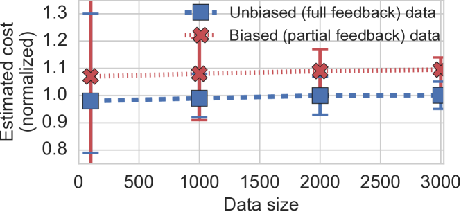
Figure 1. Counterfactual evaluation of a candidate policy using unbiased vs. biased data, based on real production data from Azure-Health. The mean estimates are normalized to the candidate policy’s true cost. Estimates based on biased data misrepresent the true cost by 9%, while estimates based on unbiased data are accurate and have lower variance. Confidence intervals are obtained by repeating the analysis on subsamples of the same size using a bootstrap procedure (Efron, 1979).

Partial feedback.  Unfortunately, implicit feedback is often one-sided—e.g., feedback is revealed for all thresholds $\leq$$X$ but not $>$$X$—making it a form of partial feedback, where each decision only reveals feedback for some of the actions. Partial feedback is inherently biased, because it generates more feedback for some actions than others, making it difficult to use for counterfactual evaluation. For example, an Azure-Health policy that always waits $\leq$$3$ min for unresponsive machines will never generate feedback for longer waiting times. As a result, any data collected from this policy cannot be used to counterfactually evaluate a candidate policy that waits 4 min or more.

Full feedback.  In contrast, full feedback arises when each decision reveals feedback for every possible action. This would be the case if the Azure-Health policy waits the maximum time (10 min) for every machine, revealing implicit feedback for all lower times as well. Such full feedback data is unbiased. Unfortunately, full feedback data is rare in threshold decisions, and typically only arises when a system is initially deployed with a very conservative policy (often to collect data that will be used to train better policies). In our work, we use full feedback data only to train initial policies, and as an idealized baseline to quantify the effects of biased data.

As an illustration of the bias problem, we take production data from an initial two-month period during which Azure-Health deployed the conservative policy of always waiting 10 min, generating an unbiased, full feedback dataset. We then derive a biased, partial feedback dataset based on a more optimized policy they used later on. We use the biased and unbiased datasets to counterfactually evaluate a new candidate policy. Figure 1 shows that the counterfactual estimate using unbiased data closely matches the true cost of the candidate policy, even when the dataset is small; with more data, the variance reduces sharply around the true cost. In contrast, when using biased data, the estimated cost deviates from the true cost by 9%, and no amount of additional data removes this bias. This is an important point: although additional data can reduce the variance of an estimate, it cannot remove the underlying bias (Langford et al., 2008). The candidate policy in this example appears to have higher cost than it truly does, which could mislead the Azure-Health team.

2.3. Existing Approaches

Many existing approaches aim to address the bias problem when counterfactually evaluating a policy, as summarized in Table 1. Here, we discuss the strengths/weaknesses of each approach in the context of threshold decisions and their implicit feedback. The high-level takeaway is that most approaches used in systems still suffer from bias. Unbiased approaches from RL give a strong starting point for Sayer, but they are are either too invasive (e.g., they require a live deployment) or are not data-efficient. In particular, no existing approach leverages implicit feedback.

	Low bias	Data efficient	Less invasive
A/B testing	✔	✘	✘
Online learning	⚪	✘	✘
Simulator	✘	✔	✔
Data-driven modeling	✘	✔	✔
Naive exploration/IPS	✔	✘	✔
Sayer	✔	✔	✔

Table 1. Different approaches for counterfactually evaluating policies that make threshold decisions (⚪ $=$ “somewhat”). Naive exploration and $\mathtt{IPS}$ allow unbiased, offline evaluation of arbitrary policies, but they fail to leverage implicit feedback like Sayer.

A/B testing is the gold standard for evaluating policies in a cloud system (Kohavi et al., 2009; Kohavi and Longbotham, 2015), but it requires deploying each candidate policy live alongside the current deployed policy, and randomly splitting traffic/requests between the policies. The data collected from an A/B test can only be used to evaluate the deployed policies, making it a costly and inefficient approach. Online learning approaches also deploy a policy in a live setting and use data collected from its decisions to continuously update the policy. Several systems (Dong et al., 2015; Dong et al., 2018; Tesauro, 2007; Mao et al., 2017; Erickson et al., 2010; Alipourfard et al., 2017) use online learning or RL algorithms that can accurately evaluate candidate policies that are very similar to the depoyed policy, but incur bias when evaluating policies that are different.

Instead of deploying policies, a simulator of the production environment can be used to evaluate arbitrary policies offline. This approach is data-efficient and non-invasive, but creating and maintaining an accurate simulator of a complex, evolving system can be as large an undertaking as the system itself (Floyd and Paxson, 2001; Bartulovic et al., 2017), making it prone to modeling biases (Floyd and Paxson, 2001).

Because of these difficulties, system designers often create data-driven models to predict the outcome of a given decision in a live system (e.g., (Jiang et al., 2016c; Tariq et al., 2008; Krishnan and Sitaraman, 2013)). In particular, many proposals train ML models to predict the outcome of an action based on all the available context, and make decisions based on these predictions (Zhu et al., 2017; Fu et al., 2021; Van Aken et al., 2017; Li et al., 2019; Zhang et al., 2019; Bingham et al., 2018; Klimovic et al., 2018; Peng et al., 2018; Venkataraman et al., 2016; Yadwadkar et al., 2017). However, a misspecified model will introduce biases, and (re)training it on partial feedback data collected when following the decisions of an earlier model will simply perpetuate these biases (see Figure 1).

Another data-driven modeling approach, currently used by the Azure-Health team, is survival analysis. Survival analysis is a statistical modeling approach that postulates a distribution over machine recovery times and uses this to predict any unobserved outcomes. This distribution is fitted to the data using right censoring, which explicitly models the probability of missing feedback to remove bias. However, such right censoring relies on the specific shape of the distribution, and a missspecification will reintroduce bias. Survival analysis also makes it harder to leverage available context when making a decision: it either requires large amounts of data to fit a distribution for each context, or fitting a more complex distribution that is more likely to be misspecified.

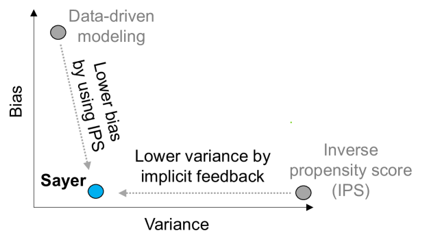
Figure 2. Sayer vs. other approaches. This figure is illustrative; actual figures appear later (e.g., 7(b)).

One way to avoid bias issues entirely is to use naive exploration, in which the deployed policy picks a random action for some fraction of the decisions, and the feedback for these exploration decisions is used to evaluate candidate policies. For example, Azure-Health currently waits the maximum time of 10 min for 35% of its decisions (revealing implicit feedback for all lower wait times), and the CFA system (Jiang et al., 2016b) for video QoE optimization collected data on a small portion of sessions by taking uniform random actions. These exploration datasets are unbiased and can hence be used to evaluate arbitrary policies offline.

By additionally recording the probability of each chosen action, a technique called Inverse Propensity Scoring ($\mathtt{IPS}$) (Horvitz and Thompson, 1952) (and more advanced variants like doubly robust estimators (Dudík et al., 2014)) can be used to leverage both the exploration decisions and the biased decisions of the deployed policy. This is because $\mathtt{IPS}$ uses probabilities to reweight (debias) the cost feedback of each action to compensate for differences in the observed frequency of actions between the deployed policy and candidate policy. This reweighted data can be used to evaluate the cost of a candidate policy, or compute updates to the policy during optimization. Although the utility of $\mathtt{IPS}$ has been recognized (Bartulovic et al., 2017; Lecuyer et al., 2017), it remains underutilized by the systems community. One reason for this may be that $\mathtt{IPS}$ requires a policy’s decisions to satisfy certain independence assumptions. Fortunately, these assumptions are naturally satisfied by the threshold decisions we study.

We note that Table 1 identifies general properties that may not hold in all situations. For example, if a threshold decision can be perfectly modeled, then a simulator or data-driven model may be unbiased. Since $\mathtt{IPS}$ comes closest to our goal, Sayer builds on $\mathtt{IPS}$ to develop a methodology that is unbiased and data-efficient. Figure 2 illustrates the expected contrast between Sayer and these prior methods.

2.4. Goals of Sayer

As explained above, randomized exploration and $\mathtt{IPS}$ provide a good foundation for Sayer, because they enable unbiased counterfactual evaluation of arbitrary policies. However, these approaches suffer from a serious limitation: they only consider feedback for the (single) action taken by a policy decision. To leverage implicit feedback, Sayer must develop new techniques that can be integrated easily into existing system policies. Specifically, Sayer addresses two challenges:

1. How do we leverage implicit feedback that is biased and outcome-dependent?  Sayer develops a new counterfactual estimator for implicit feedback (§3.2) that is supported by new implicit exploration and data logging techniques (§3.3).

2. How do we incorporate implicit feedback into the lifecycle of a system policy?  Sayer modifies existing components of a system policy’s workflow (§3.1) while supporting its continuous optimization lifecycle (§3.3).

We focus on threshold decisions that satisfy the independence assumptions mentioned above; for more complex decisions, $\mathtt{IPS}$ and Sayer may not be appropriate (see §6). We evaluate Sayer in two production systems in Azure (§4.2,§4.3) using real production data and prototypes that mimic the production systems.

3. Design of Sayer

This section presents the design of Sayer. We state Sayer’s assumptions and overview its architecture, and then present the key technical idea that enables unbiased counterfactual evaluation based on implicit feedback. We then show how Sayer integrates with the lifecycle of a system policy.

3.1. Overview

Terminology and assumptions.  A system policy ($\pi$) makes decisions by taking the context ($\vec{x}$) of a decision as input and choosing a single action ($\pi(\vec{x})$) to take from a set of allowed actions. The context $\vec{x}$ comprises properties of the environment or the system state that are considered relevant to the decision. Traditionally, when the policy takes an action, we observe the cost (feedback) $c(\pi(\vec{x}))$ associated with that action. But as observed in §2.1, in system policies that make threshold decisions, we can deduce the cost of more actions than the one we actually take, i.e., implicit feedback.

We make three assumptions that are relevant to the system policies we study. First, we assume that the decisions made by a policy are mutually independent. This assumption corresponds to the contextual bandits setting (Langford and Zhang, 2007; Dudik et al., 2011) and is required by the $\mathtt{IPS}$ estimator we build on. Intuitively, it means that the action chosen by the system policy at a given time does not influence the cost of future actions. For instance, such a long-term influence could arise if an action drastically changes the load of the system, thereby changing the future distribution of contexts; or by changing the state of a cache, thereby changing the cost of a future action with the same context. Fortunately, the independence assumption is a good model for the threshold decisions in §2.1, as they involve one-step decisions in large enough systems that the impact of individual decisions are well isolated.

Second, we assume the policy makes a one-dimensional, discrete decision. That is, the actions are the (multiple) possible values for a single parameter. This is a standard assumption in the learning literature we build on, where exploring continuous, unbounded, or complex action spaces quickly becomes intractable without strong structure (Swaminathan et al., 2016). When the action space is continuous, as in our Azure-Health example, we can discretize the possible actions within a chosen range, e.g., between 0 and a maximum wait time fixed a priori. This restriction does not apply to the context or cost function, which may be continuous and multi-dimensional.

Third, we assume that the observed potential outcomes do not depend on the chosen action. This assumptions is a direct extension of the inclusion restriction assumption from causal inference (Imbens and Rubin, 2015) to our implicit feedback setting. More concretely, it means that in Azure-Health, the recovery state of a machine after waiting for $t$ does not depend on whether the reboot timeout is set to $t+1$ or $t+10$. This is a natural assumption, because the timeout is never acted on until the actual reboot. In the Azure-Scale application, though, over-allocating by ten or twenty VMs could yield different completion times for a particular VM (e.g., due to queueing effects), violating the assumption. Fortunately, we verify that the assumption holds in practice (§4.3, Figure 9).

Finally, the contextual bandit literature typically also assumes that contexts and costs come from stationary distributions. This enables bandit algorithms to gradually learn the distribution and decrease exploration over time. However, practical system deployments often experience context and cost distributions that change over time. In this work, we thus focus on continuous exploration, which allows us to cope with this kind of non-stationarity.

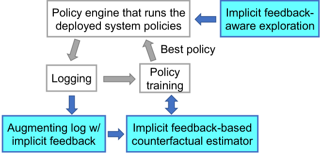
Figure 3. Architecture of Sayer. Sayer expands the traditional policy optimization workflow by adding three new modules (highlighted in blue) that leverage the available implicit feedback.

Architecture.  Figure 3 shows the architecture of Sayer. The gray boxes are standard components of a decision-making system, which include: a policy engine that hosts the deployed policy and invokes it on every decision to obtain the policy’s chosen action, a logging component that records the outcome (cost) of each decision, and a policy training component that updates the policy based on the logged data. Sayer adds the outlined blue boxes, which we describe in detail in §3.3. The added components can be integrated seamlessly into an existing system. For example, Sayer’s implicit exploration adds some randomization to the deployed policy’s decisions, but this does not change the policy deployment interface. Similarly, existing logging components typically already log extensive information about each decision (e.g., context, action, and cost); Sayer additionally logs information about the randomization added by the implicit exploration component (in the form of action probabilities). Sayer uses this information to augment the traces output by the logging component with implicit feedback, which is done as a separate post-processing step.

The key component of Sayer is an unbiased counterfactual estimator that uses the implicit feedback augmented in the logged data of the deployed policy, to estimate the cost of an arbitrary candidate policy on the same sequence of decisions.

3.2. Implicit feedback-based counterfactual estimator

We present our algorithm for implicit feedback-based counterfactual estimation in a progressive fashion, starting from a basic framework that guarantees unbiased estimation.

In the simplest setting where a policy only receives feedback for the single chosen action, also called bandit feedback, the data collected will be biased. Here, $\mathtt{IPS}$ provides a framework for unbiased estimation.

$\mathtt{IPS}$: Unbiased estimator for bandit feedback.  To remove bias from a log of bandit feedback data, a classic solution is to log the probability ($p$) of the action being chosen alongside the context, action, and cost of the decision, yielding a tuple $(\vec{x},a,c,p)$. Based on this log, a technique called Inverse Propensity Scoring ($\mathtt{IPS}$) (Horvitz and Thompson, 1952) can then provide an unbiased estimator for any candidate policy $\pi$:

$$\mathtt{IPS}(\pi)=\textstyle\tfrac{1}{N}~{}\sum_{\begin{subarray}{c}(\vec{x},a,c,p)\end{subarray}}\frac{\mathbb{1}\{\pi(\vec{x})=a\}}{p}c.$$

$\mathtt{IPS}$ finds instances in the trace where $\pi$ chooses the same action as the deployed policy, i.e., $\pi(\vec{x})=a$ (the indicator function $\mathbb{1}$ has value $1$ under a match and $0$ otherwise). But instead of simply adding the associated cost under a match, it re-weights it by the inverse of the probability ($p$) that $a$ was chosen. Thus if $a$ has low probability, i.e., it is rarely chosen by the deployed policy, $\mathtt{IPS}$ will upweight it to compensate for the fact that $a$ is underrepresented in the trace.

Implicit feedback vs. bandit feedback.  $\mathtt{IPS}$ is an unbiased estimator for bandit feedback, but it completely ignores any feedback that may be received for actions other than $a$, i.e., implicit feedback. Implicit feedback thus provides a type of partial feedback that lies between full feedback and bandit feedback. Although partial feedback has previously been studied using feedback graphs (Mannor and Shamir, 2011; Alon et al., 2013), those algorithms take a fixed feedback graph as input and optimize one policy online. In contrast, we are concerned with counterfactual evaluation of many policies, and the feedback we receive depends on the outcome of each decision. For example, in Azure-Health, if a machine responds at time $\tau$ before the chosen wait time $a$, we obtain full feedback, but if it does not, we only obtain feedback for actions $\leq a$. This is illustrated in Figure 4. Since $\mathtt{IPS}$ requires a probability $p$ that is fixed in advance, it does not support such variable feedback out of the box.

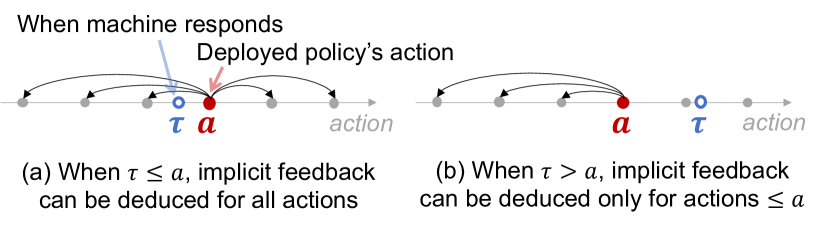
Figure 4. Implicit feedback example. Each black arrow indicates that the feedback of an action can be deduced from the feedback of the deployed policy’s action. Importantly, implicit feedback is outcome-dependent: if a machine responds (at $\tau$) before the chosen wait time $a$, we obtain full feedback, but otherwise we only obtain feedback for actions $\leq a$.

So how do we incorporate implicit feedback into $\mathtt{IPS}$ without compromising its unbiasedness?

$\mathtt{Implicit}$: Unbiased estimator for implicit feedback.  Our key insight is that $\mathtt{IPS}$ can be interpreted as matching datapoints in the trace according to an event $E$ under which we (1) know the cost feedback and (2) can compute the probability that $E$ occurs, $P(E)$, in order to reweight the cost. We can thus abstract $\mathtt{IPS}$ to obtain a template for our estimator:

$$\mathtt{Implicit}(\pi)=\textstyle\tfrac{1}{N}~{}\sum_{\begin{subarray}{c}(\vec{x},a,c,\vec{p})\end{subarray}}\frac{\mathbb{1}\{E\}}{P(E)}c(\pi(\vec{x})).$$

In the original $\mathtt{IPS}$ estimator, $E=\{\pi(\vec{x})=a\}$ is the event that the chosen actions match. $P(E)=p$ since the actions match precisely when the deployed policy chooses $a$.

Now, by redefining $E$ to be a larger event, we can match a larger set of points, while preserving the unbiasedness of this template! In particular, Sayer defines $E$ as the event that “the feedback of the candidate policy’s action $\pi(\vec{x})$ can be deduced from the outcome of the deployed policy’s action $a$”. Intuitively, $\mathbb{1}\{E\}$ is 1 only if the feedback $c(\pi(\vec{x}))$ is available, either explicitly through matching, or implicitly through deduction from the outcome of action $a$ recorded in the trace. Figure 4 illustrates an example. $P(E)$ is then the probability that the deployed policy chooses an action whose outcome will allow the feedback $c(\pi(\vec{x}))$ to be deduced.

To make this more concrete, we derive $E$ and $P(E)$ for Azure-Health. The application to Azure-Scale is similar.

Applying $\mathtt{Implicit}$ to Azure-Health.  We define $E$ based on a given chosen action (wait time) $a$, its outcome (either the machine responds at time $\tau\leq a$, or it times out), and a new action chosen by the candidate policy, $\pi(\vec{x})$. The event that $\pi(\vec{x})$’s feedback can be deduced is:

$$E=\{\pi(\vec{x})\leq a\}\cup\{\tau\leq a\}.$$

The first term follows from the property of Azure-Health’s decisions that when $\pi(\vec{x})\leq a$, $c(\pi(\vec{x}))$ can always be deduced (see Figure 4). Otherwise, $c(\pi(\vec{x}))$ can be deduced only when $\tau\leq a$ (Figure 4(a)). In other words, the only case when feedback is not available is when the deployed policy’s action $a$ causes a timeout (i.e., $\tau>a$) and the candidate policy chooses to wait even longer $\pi(\vec{x})>a$. The recorded outcome does not provide any information in this case.

Next, whenever $\mathbb{1}\{E\}=1$, we need to compute $P(E)$ as well as the cost of the candidate policy’s action $c(\pi(\vec{x}))$. There are four cases, as illustrated in Figure 5.

• Case 1: $a\geq\tau$ and $\tau>\pi(\vec{x})$. In this case, $\pi(\vec{x})$ will cause the machine to reboot, so $c(\pi(\vec{x}))=\pi(\vec{x})+R$, where $R$ is the the fixed reboot delay cost (see §4.2 for details). Moreover, this information is available if and only if the deployed policy chooses an action $\geq\pi(\vec{x})$, so $P(E)=P(a\geq\pi(\vec{x}))=\sum_{a^{\prime}\geq\pi(\vec{x})}p(a^{\prime})$.

• Case 2: $a\geq\tau$ and $\pi(\vec{x})\geq\tau$, which means both deployed and candidate policies will wait long enough for the machine to respond, so $c(\pi(\vec{x}))=\tau$. This information is available if and only if the deployed policy chooses an action $\geq\tau$, so $P(E)=P(a\geq\tau)=\sum_{a^{\prime}\geq\tau}p(a^{\prime})$.

• Case 3: $\tau>a$ and $a\geq\pi(\vec{x})$, which means that the deployed policy’s action is not long enough for the machine to respond before rebooting, and the candidate policy chooses to wait even less time. So $c(\pi(\vec{x}))=\pi(\vec{x})+R$. This information is available if and only if the deployed policy’s action is greater than the candidate policy’s action, so $P(E)=P(a\geq\pi(\vec{x}))=\sum_{a^{\prime}\geq\pi(\vec{x})}p(a^{\prime})$.

• Case 4: $\pi(\vec{x})>a$ and $\tau>a$, which means $E$ is false and $\mathbb{1}\{E\}=0$, so we do not need to compute anything.

Unbiasedness and low variance of  $\mathtt{Implicit}$.  $\mathtt{Implicit}$’s unbiasedness follows directly from that of $\mathtt{IPS}$. Given a datapoint $(\vec{x},\vec{c})$ and the action $a$ chosen by the policy that was deployed at the time, we have:

$$\mathbb{E}\Big{(}\frac{\mathbb{1}\{E\}}{P(E)}c(\pi(\vec{x}))\Big{)}=\frac{\cancel{\mathbb{E}\big{(}\mathbb{1}\{E\}\big{)}}}{\cancel{P(E)}}c(\pi(\vec{x})),$$

implying that $\mathbb{E}\big{(}\mathtt{Implicit}(\pi)\big{)}=c(\pi(\vec{x}))$, and hence that $\mathtt{Implicit}$ is an unbiased estimate of the cost of policy $\pi$, had it run on the same sequence of datapoints observed during data collection. We can see that $P(E)$, which we call the implicit probability, plays a key role in this unbiasedness guarantee. Indeed, reweighting the implicit feedback deduced from matched events by $1/P(E)$, similar to $\mathtt{IPS}$’s reweighting by $1/p$, cancels out the $\mathbb{E}\big{(}\mathbb{1}\{E\}\big{)}$ term in the expectation, thereby removing the bias due to missing information.

In addition, $P(E)$ lowers the variance of $\mathtt{Implicit}$’s estimates, as compared to $\mathtt{IPS}$. Computing the variance yields:

(1) $$\mathbb{V}\Big{(}\frac{\mathbb{1}\{E\}}{P(E)}c(\pi(\vec{x}))\Big{)}=\frac{1-P(E)}{P(E)}c(\pi(\vec{x}))^{2}.$$

As we can see, the variance of the cost is scaled by $1/P(E)$. In $\mathtt{IPS}$, the weight $1/p$ can be quite high when the deployed policy and candidate policy differ. In contrast, $\mathtt{Implicit}$ matches a range of actions and $P(E)$ is their total probability; this leads to larger values of $P(E)$ and hence lower variance.

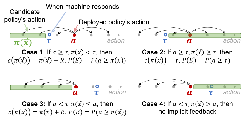
Figure 5. Example of how to calculate $c(\pi(\vec{x}))$ and $P(E)$ based on implicit feedback in Azure-Health.

3.3. Implicit feedback-based policy optimization

We now discuss the system components of Sayer (Figure 3), which integrate the implicit counterfactual estimator above into the lifecycle of system policy optimization.

Implicit data augmentation.  Sayer’s logging component ensures that the information of each decision is recorded correctly, so that the generated traces can be used for counterfactual evaluation and training. In a standard bandit feedback setting, the logging component would log the tuple $(\vec{x},a,c,p)$, where $\vec{x}$ is the input context, $a$ the chosen action, $c$ the cost feedback received for $a$, and $p$ the probability of choosing $a$. In Sayer, since there is implicit feedback, we additionally log the implicit probability and cost of all actions whose feedback can be deduced, i.e., $(\vec{x},\{(a_{i},c_{i},p_{i})\}_{i})$. This information is used by our implicit counterfactual estimator to correctly handle implicit feedback. In Azure-Health, for example, if a logged action $a=5$ min leads to a machine responding at $\tau=3$ min, then instead of logging $(\vec{x},5~{}\textrm{min},3~{}\textrm{min},p)$, we augment the entry with implicit feedback (using Case 1 and Case 2 in Figure 5): $(\vec{x},\{(a<3~{}\textrm{min},(a+R)~{}\textrm{min},P(a<3~{}\textrm{min})),(a\geq 3~{}\textrm{min},3~{}\textrm{min},P(a\geq 3~{}\textrm{min}))\})$.

Counterfactual estimation and policy training.  Given the logged data augmented with implicit feedback and probabilities, Sayer uses its implicit counterfactual estimator to evaluate and train new policies. To train a policy, Sayer uses a class of contextual bandit learning algorithms that internally use estimators such as $\mathtt{IPS}$ to efficiently search a policy space (Dudik et al., 2011), but replaces the internal estimator with $\mathtt{Implicit}$. Sayer follows the common practice of splitting the logged data into a train set (to learn the new policy) and a test set (to evaluate it); the difference is that Sayer uses counterfactual training and evaluation algorithms, to ensure unbiasedness. The granularity at which Sayer is run, and the subset of data used to train and test, is largely orthogonal to our work. For example, in our evaluation we run Sayer in a “batch retraining” mode, where a new policy is periodically trained from scratch on a trailing window of data, before being counterfactually evaluated on the most recent data.

By repeating the above process, Sayer enables a continuous optimization loop that allows a system policy to evolve. Continuous optimization is necessary to cope with changes or non-stationarity in the system or environment (§4.2,§4.3).

Implicit exploration and logging.  To enable unbiased counterfactual estimation, and to cope with non-stationarity, Sayer includes an exploration component that adds controlled randomization to the deployed policy’s decisions. This ensures that feedback is received for all actions, not just those deemed optimal by the deployed policy (the classic exploration-exploitation tradeoff). A simple algorithm for exploration is $\mathtt{EpsilonGreedy}$ (Langford and Zhang, 2007), which selects a random action $\epsilon$ fraction of the time and uses the action chosen by the deployed policy the remaining $1-\epsilon$ fraction of the time.

Randomizing over all actions makes sense when feedback is only received for the chosen action (i.e., bandit feedback). However, this means that the probability of choosing an action can be as low as $p=\epsilon/a$, yielding high variance (see Equation 1) even with a large fraction of exploration actions. In our setting, where we receive implicit feedback for other actions, randomizing over all actions “underutilizes” this feedback. Instead, Sayer explores by selecting the maximal action, i.e., the action that yields the most feedback. For example, in Azure-Health, this corresponds to waiting 10 min in each explore step. Using the maximal action for exploration means that the minimal observation probability is $P(E)=\epsilon$, reducing the variance of our counterfactual estimator and supporting smaller amounts of exploration. Thus for a given exploration budget, Sayer’s implicit exploration technique better utilizes implicit feedback. This is particularly important to enable continuous exploration at low cost.

Of course, exploring using the maximal action may not always be desirable, especially if that action is likely to be costly. We use this heuristic because it allows us to explore less frequently, and because in our applications the maximal action is a reasonable default action that we are trying to improve upon. An alternative would be to explore randomly over the action space using a distribution that accounts for the desirability of each action. However, this would require more frequent exploration, and would not completely avoid exploring the maximal action, which is necessary to collect unbiased data.

4. Evaluation

We now demonstrate the value of Sayer in two real applications from Azure—Azure-Health and Azure-Scale. Using a combination of simulation (driven by full-feedback traces and synthetically generated traces) and A/B testing in a live prototype, we show that (i) compared to baseline performance estimators, Sayer’s $\mathtt{Implicit}$ counterfactual estimator is unbiased and has lower variance; and (ii) the more accurate counterfactual estimation allows Sayer to train better system policies than the baselines, even though Sayer incurs the cost of exploration.

4.1. Methodology

We define the baselines and performance metrics common to both applications here. In §4.2 and §4.3, we introduce the details of each application.

Baseline estimators.  Given a log of $(\vec{x},a,c,p)$ tuples, we consider four baseline performance estimators for counterfactual evaluation and optimization:

• Direct Method uses the log to train a linear model using Vowpal Wabbit ($\mathtt{VW}$) (Vowpal Wabbit, [n.d.]), a state-of-the-art bandit library, that predicts the cost of any context and action. This can be viewed as a data-driven performance modeling baseline, which may be biased by the log and the model. The cost model is used to predict missing information when doing counterfactual evaluation, and when training a new policy.

• Survival Analysis postulates a distribution over the outcomes for all decisions (e.g., the distribution of machine recovery times). Like the Azure-Health team, we fit a right-censored Lomax (long tail) distribution using maximum likelihood estimation (implemented with Pyro (Bingham et al., 2018)). Right censoring accounts for unobserved costs by putting all the probability mass of the tail on the maximum observed value. We fit this distribution on all observations, since conditioning on features reduces the amount of data and yields poor performance. Missing costs are replaced with their expected value for counterfactual evaluation, and the learned policy is the action with the lowest expected cost.

• $\mathtt{IPS}$ is described in §3.2. This classic counterfactual estimator is well known to be unbiased, but has high variance and does not leverage implicit feedback. It is used both for counterfactual estimation, and to debias the cost during policy optimization using $\mathtt{VW}$ (Vowpal Wabbit, [n.d.]).

• Naive Implicit is the Direct Method trained on the log augmented with implicit feedback (like Sayer), but without using implicit probabilities. It can be viewed as using implicit feedback without proper reweighting, and is used to emphasize the importance of reweighting to remove bias.

Baseline policies.  To ensure fairness, all policies use the same training interface of $\mathtt{VW}$ (which accepts as input a log of $(\vec{x},a,c,p)$ tuples augmented by each estimator) and train the same model (a linear contextual bandit policy)—except Survival Analysis, which is a different type of model. This process yields five policies: { Sayer, Direct Method, Survival Analysis, $\mathtt{IPS}$, Naive Implicit }-based policies. These policies use different exploration strategies: Direct Method always uses the action returned by the trained policy; for a random $\epsilon$ fraction of decisions, Sayer and Naive Implicit use the maximal, full-feedback action (since both use implicit feedback), while $\mathtt{IPS}$ uses a random action (since it only matches the exact action).

We also include two baselines that are not continuously updated, but serve as useful reference design points:

• Full-feedback (v0) policy chooses the most conservative action and obtains full feedback. It maximizes information in the collected data at the cost of performance.

• One-shot learning (v1) policy feeds the full-feedback data (from which we can deduce the true outcome of every action) to $\mathtt{VW}$ to train a policy, but never updates the policy.

Finally, a skyline policy shows an upper bound on the performance one can hope to achieve with our $\mathtt{VW}$ model:

• Omniscient is a policy trained on full-feedback data, even when such feedback would not be available from the data collection. This is only available in setups where we have access to full feedback, and simulate partial feedback by hiding information.

Metrics.  We compare these approaches under a continuous optimization scenario, in which trained policies are deployed, and updated using a rolling window of data collected while they were running. We focus on the following metrics:

• Trained policy cost: Each system defines a cost associated with policy actions. We measure the cost of running a trained policy (lower is better).

• Counterfactual evaluation error: Using data collected when running the policy, we measure the difference between the estimated cost for a different candidate policy, and the true value for this cost.

For each metric we show both the average performance (cost), as well as the range of values that can happen due to randomness in the data. These ranges are computed using bootstrap (Efron, 1979), a common resampling technique from statistics analogous to averaging over repeated experiments, which gives a sense of the variance in our results.

4.2. Application I: Azure-Health

Azure-Health is a monitoring service that uses heartbeats to detect unresponsive physical machines within datacenters, and is responsible for rebooting unresponsive machines after a threshold amount of time. We formalize the problem as follows: faced with an unresponsive physical machine, the policy chooses a wait time amongst ten options (the action set) {1,2,…,10} min, before rebooting the machine. This maximum wait of 10 minutes is a practical limit imposed by the Azure-Health team, regardless of any RL constraints. The decision is based on a number of context features for the machine, collected via an existing telemetry pipeline, and available to the policy at decision time. This context includes the hardware/OS configuration of the machine, which cluster it belongs to, the number of previous failures in the cluster, and the number of client VMs running on the machine. The cost of an action $a$ is the total downtime experienced by customer VMs. It is calculated as the recovery time $\tau$, plus a fixed reboot time $R=10~{}\textrm{min}$ if the server is rebooted ($a<\tau$), scaled by the number of VMs on the server $N_{\textrm{VMs}}$:

$$cost=N_{\textrm{VMs}}\Big{(}\mathbb{1}\{a<\tau\}\tau+(1-\mathbb{1}\{a<\tau\})(a+R)\Big{)}$$

As explained in §3.2, Azure-Health provides implicit feedback. Choosing action $a$ reveals the cost of all actions $a^{\prime}\leq a$, as we know the corresponding state of the machine. If we observe a recovery ($a\geq\tau$), we can also deduce the cost of every action, making it full feedback.

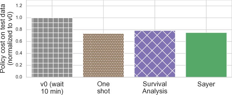
Figure 6. First training period: We use the 2nd split (S2) to compare the performance of policies trained on the 1st split (S1), relative to the v0 policy.

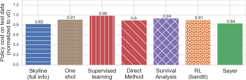
(a) Cost of policies trained by various estimators (x-axis).

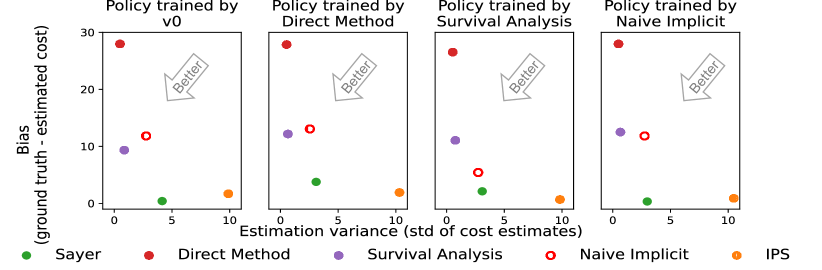
(b) Counterfactual estimation error (bias & variance) on 7(a) policies.

Figure 7. Policy optimization and evaluation over time. All plots show costs (downtime) normalized to the cost of the default policy (v0). (7(a)) shows the performance of policies retrained from data they generated in S2, when evaluated on S3. (7(b)) shows the counterfactual estimate (one colored dot per estimator) of how the policies from 7(a) (one per box) would perform on S3, using data collected by deploying the v1 policy, normalized to the full-feedback ground truth. Sayer achieves both unbiased and low variance cost estimates, which trains better policies (7(a)).

4.2.1. Trace-driven simulation

We obtained a production trace of $13.5k$ events with full feedback from Azure-Health, collected during an initial two-month period when the team deployed the conservative policy of always waiting the maximum of 10 min. Based on this trace, we can compute the ground truth performance of different policies, and thereby evaluate the performance of Sayer’s counterfactual estimator and its trained policies. We split the production trace into three periods, each with 3000-5000 data points, corresponding to environmental changes:

• S1 corresponds to the phasing out of a hardware configuration (a specific server SKU),

• S2 lies between the events of S1 and S3, and

• S3 corresponds to a major software upgrade.

Because these hardware and software configuration changes affect large portions of the machines, we also expect them to affect the machine’s recovery times and the relationship between observed features and recovery times, which we observe in the data. We leverage these three phases to evaluate how different approaches cope with environmental changes compared to Sayer.

First training period.  First, without any prior knowledge, we start with v0 (choosing the maximal wait time of 10 minutes) in S1, which produces full feedback, train new policies according to the different approaches described in §4.1, and evaluate these policies in S2. Figure 6 shows the results. The policies trained by estimators Direct Method, Naive Implicit, and v1 will be identical on full feedback. They yield a $26.5\%$ improvement over the v0 baseline policy. On S1, Sayer will learn the same policy, but is slightly less efficient because of the added exploration, which chooses the maximal action on $10\%$ of the actions. Despite this exploration, Sayer yields a $25\%$ improvement over the v0 baseline. Survival Analysis is less expressive, as it chooses a single wait time for all machines, but it still yields a $21\%$ improvement (alternatively, we could train one model per cluster to take features into account, but this degrades the results due to the small data).

Continuous training.  Second, we evaluate different policy training approaches in a dynamic setting by deploying each policy on S2 (yielding the performance from Figure 6), collecting the resulting feedback, and retraining each policy on the data generated while it was running. For instance, if a policy waits $3$ min for a machine, we only show the costs for actions $a\leq 3$ in case of a reboot, and all costs if the machine recovers within that time frame. This partial feedback data is used to train the new policy, which is then evaluated on S3. Figure 7(a) shows the policy cost for each of these retrained policies, measured on S3 using full feedback. There are several observations about Sayer’s performance:

• Substantial benefits by continuous retraining: As we see in Figure 7(a), the Omniscient skyline policy, which trains its policy on S2 with full feedback, yields a $15.5\%$ improvement over v0 when deployed on S3. However, keeping the one shot model trained on S1 only gives an $8.6\%$ improvement. We expect even larger degradation as the environment evolves.

• Benefits of implicit exploration: Naively retraining on data collected when running an optimized policy (i.e., without exploration) is suboptimal. Figure 7(a) shows that training a policy with Naive Implicit, which ignores missing feedback from a lack of exploration, is almost as bad as v0. Even extrapolating missing feedback using Direct Method or Survival Analysis (which does improve performance to $7.6\%$ and $6.1\%$, respectively) is still short of the v1 baseline (trained on older but full feedback data). Sayer is the only one to reach Omniscient’s performance, again with a small added cost for exploration, yielding a $14.7\%$ improvement.

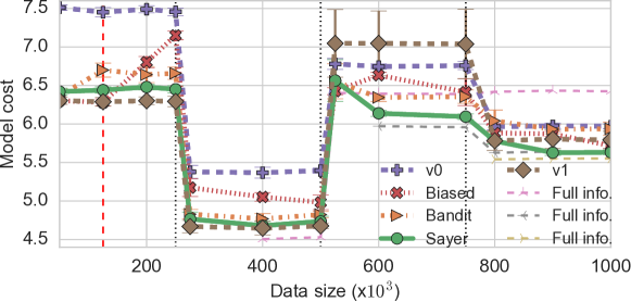
(a) Evolution of performance.

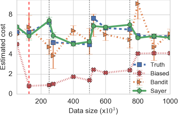
(b) Counterfactual evaluation.

Figure 8. Behavior of periodic optimization and counterfactual evaluation. The red vertical line shows when policies start being updated based on the data they collect. The black vertical lines show environment changes (the generator is trained on a different part of our data trace).

Counterfactual estimation accuracy.  Next, Figure 7(b) evaluates the accuracy of various counterfactual estimators. Counterfactual estimators can be used to evaluate any candidate policy, based on data collected when running a different policy. To evaluate this capability, we use all our policies trained on S2, and evaluate their respective performance on S3 (boxes in Figure 7(b)) according to each counterfactual estimator (colored dots in Figure 7(b)), using data collected while running v1. Comparing these counterfactual results to the true (full information) cost, we can compute the bias (expected error) and variance of each counterfactual estimator. Accurate estimators can help operators distinguish good policies from bad ones without running the policies, based on data collected by the deployed policy.

• Not accounting for missed feedback causes significant bias: Direct Method, Naive Implicit, and Survival Analysis have mean estimates far away from the truth, even if they try to fill the gap of missing information (Direct Method and Survival Analysis). All three approaches also reverse the order of Sayer and other policies (not shown), resulting in a misleading assessment of their relative performance, and deploying a potentially worse policy if this assessment is acted on. In contrast, Sayer and $\mathtt{IPS}$ use exploration and thus yield unbiased estimates when evaluated on multiple, varied policies.

• Implicit feedback reduces variance: $\mathtt{IPS}$, which uses exploration, also yields unbiased counterfactual estimates of a policy’s cost, but compared to Sayer ($\mathtt{Implicit}$ estimator), the variance of the estimate is much higher. This also implies poorer training performance, with the trained policy yielding similar results to the one shot model ($8.5\%$ improvement over v0) in Figure 7(a).

4.2.2. Microbenchmarking using synthetic traces

We also generate simulated traces inspired by the real dataset, in order to evaluate Sayer in the face of non-stationarity, when periodically retraining policies on a trailing window of data. Our goal is not to model the real world exactly; instead, our goal is to show how the different counterfactual analysis techniques deal with non-stationarity.

For realism, we learn the simulator’s parameters from our production data as follows. We draw from a Bernoulli distribution to determine if the machine is suffering from a temporary outage or a failure. For temporary outages, we draw $\tau$ from a Beta distribution with support in $[0,10]$. We create six scenarios by clustering recorded failures at different racks within a data center, and using the distribution of their recovery times in the full feedback data to learn the parameters for the Bernoulli and Beta distributions for each cluster. The clusters correspond to different probabilities of recovery, and longer/shorter tails in recovery time. We learn one such generator for each of the four splits in the trace described in §4.2.1. By switching from one generator to the next, we simulate a change in the environment. Policies are initially trained on full feedback data, and then periodically retrained using a trailing window of the last $20k$ data points using only the data they observe. They are unaware of environment changes other than through the data. Policies with exploration use an exploration rate of $10\%$.

Figure 8(a) shows the average downtime (cost) of the best performing baselines in Figure 7(a): $\mathtt{IPS}$, Direct Method, and v1. Environmental changes are shown by the three vertical dotted black lines. The Omniscient lines show the performance of an omniscient policy based on full-feedback data started at the beginning of each period. These are upper bounds on performance in their starting environment, but often degrade after environment changes.

Once again, deploying a policy without exploiting implicit feedback (i.e., $\mathtt{IPS}$) or not accounting for implicit feedback properly (i.e., Naive Implicit) leads to poor performance that is often closer to the v0 policy than to the omniscient one. The implicit feedback available to Sayer allows it to outperform the $\mathtt{IPS}$-based policies by 3-18%, depending on the environment. Sayer is also competitive with the Omniscient policy, increasing downtime by only $3\%$, a relatively low cost. Finally, the v1 policy performs competitively in the first and second environments, but significantly underperforms in the third environment with a downtime of $7$ minutes, demonstrating the need for periodic retraining.

Figure 8(b) shows the accuracy of counterfactual performance estimation on a single policy, using data generated by different deployed policies from the previous data window. The bias of Naive Implicit again leads to an underestimate of up to $3\textrm{x}$. Compared to $\mathtt{IPS}$, which is also unbiased, Sayer provides a significant reduction in variance (as shown by the bootstrap bars), allowing accurate estimation within smaller time windows. This potentially reduces the time that stale models remain deployed in production environments.

4.3. Application II: Azure-Scale

Azure-Scale serves user requests to scale up a group of VMs by a given amount. When a user requests $k$ new VMs of a given type, to ensure the timely creation of these VMs, Azure-Scale over-allocates by creating $k+a$ VMs, and returns the first $k$ that are created. In this application, the goal is to trade off the resource cost of over-allocating VMs with the completion time $t$ of a requested group of VMs. The over-allocation $a$ should be minimized to save resources, while being high enough to meet Service Level Objectives (SLOs) such as low median response time (MRT). The default, conservative over-allocation policy (v0) deployed in Azure-Scale always chooses $a=0.2k$ (or $a=k$ when $k$ is small, i.e. $\leq 4$), and any over-allocation is capped to $0.2k$ (or $k$ when $k$ is small, i.e. $\leq 4$).

We use two possible cost metrics that capture this trade-off in Azure-Scale. The first cost trades off meeting the MRT SLO with the over-allocation cost, formalized as:

$$cost1=1\{t>MRT\}\cdot\min(t-MRT,max\_cost)+\gamma\cdot a$$

where $MRT$ is the SLO objective (we use $80$ sec), $t$ is the creation completion time of the group of VMs, $max\_cost$ bounds the cost for stability (we use $100s$), and $\gamma$ is a factor to put $t$ and $a$ on the same scale (we use $13$). Cost1 penalizes actions that miss the SLO ($t>MRT$) linearly up to $max\_cost$, while each over-allocated VM “costs” $\gamma$. This cost enables implicit feedback in two forms. First, observing an over-allocation of $a$ VMs and their completion times gives feedback for all over-allocations $a^{\prime}\leq a$, since $t$ is known for every $a^{\prime}$ (but not for any $a^{\prime\prime}\geq a$). Second, full feedback for every $a$ is given if $t\leq MRT$, since the first term of the cost that includes $t$ is removed by the indicator function.

We also use an alternative cost function with less implicit feedback:

$$cost2=\min\Big{(}max\_cost,0.99\cdot\max(0,t-MRT)$$

$$+0.01\cdot\max(0,MRT-t)+\gamma\cdot a\Big{)}.$$

Here, both missing the $MRT$ and meeting the $MRT$ by too much are penalized, though with a smaller coefficient for meeting the $MRT$. This cost receives less implicit feedback, because the information of larger actions is not revealed even when $t\leq MRT$, since we do not observe completion times for VMs we never created. The only way to get full feedback is to choose the highest possible action.

To enable experimentation with different over-allocation policies, we build a prototype which mimics the functionality of Azure-Scale, using the public interface of Azure. The prototype receives requests for $k$ VMs of a given type, decides on an over-allocation number ($a$), and issues $k+a$ VM creations to Azure. It returns a completion time that is the $k^{th}$ smallest VM creation time to the user. Unlike the production system, however, it also waits for all $k+a$ requests to complete and logs each completion time before deleting the additional VMs. We use our prototype to replay an Azure-Scale production trace spanning 4 weeks, and containing 43821 requests made by a small subset of users to a North-American datacenter. Requests are capped at $100$ new VMs, but most requests are small ($1$ to $8$ VMs). The trace logs the request’s timestamp, type of VM, and the over-allocation determined by the currently deployed policy.

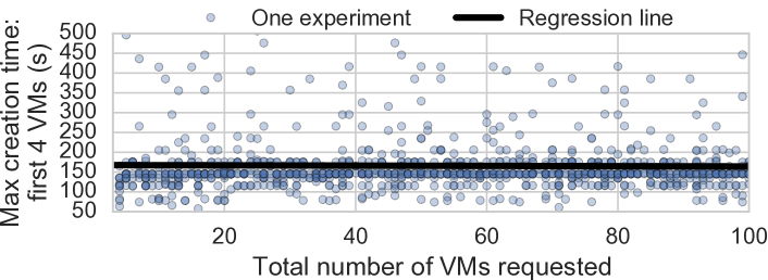
Figure 9. Assumption verified: no significant influence of number of requested VMs on the completion times.

Observed potential outcomes assumption.  Before we dive into the results, we first validate Sayer’s observed potential outcomes assumption. In the context of Azure-Scale, implicit feedback could be unreliable if the system batches requests before starting allocations, and uses an allocation logic that depends on batch size. We designed a randomized experiment to empirically verify that the completion time of $k$ VMs out of the first $k+a^{\prime}$ is the same whether we request $k+a^{\prime}$ or $k+a,a>a^{\prime}$. We sent $1000$ requests each with a randomly assigned total number of VMs ($k+a\in[1,100]$, the maximum in our trace) and VM type, and analyzed the impact of the total requested number on the completion time of $k$ VMs out of $k+a^{\prime}$. Figure 9 shows a representative example, for $k=4,a^{\prime}=0$. For each value of $k$ and $a^{\prime}$, we run a statistical test using a regression, and find no significant influence of total number of requests on the completion times: the slope of the regression is close to $0$, and the p-value is high, meaning that the data is compatible with our assumption.

4.3.1. Trace-driven simulation

We start by collecting a full feedback trace using our prototype, and split the resulting data into a training and testing set, each containing two weeks worth of data. We perform both policy optimization and counterfactual evaluation to test Sayer. The key observations are as follows, which largely corroborate the takeaways from Azure-Health.

Impact of implicit feedback.  To showcase the different values of implicit feedback, we use Sayer to train two policies, one to optimize cost1 (providing more implicit feedback) and the other for cost2 (providing less implicit feedback), respectively. We train each policy using the log generated from a common Naive Implicit policy, with $10\%$ of exploration, on increasing amounts of training data from the first split, and evaluate their performance with full feedback on the second split. Figure 10 shows that Policy1, by leveraging implicit feedback, improves faster and performs better than Policy2 over the same amount of training data, showing 8.4% and 6.3% better performance in terms of cost1 and cost2 when all the training data is used.

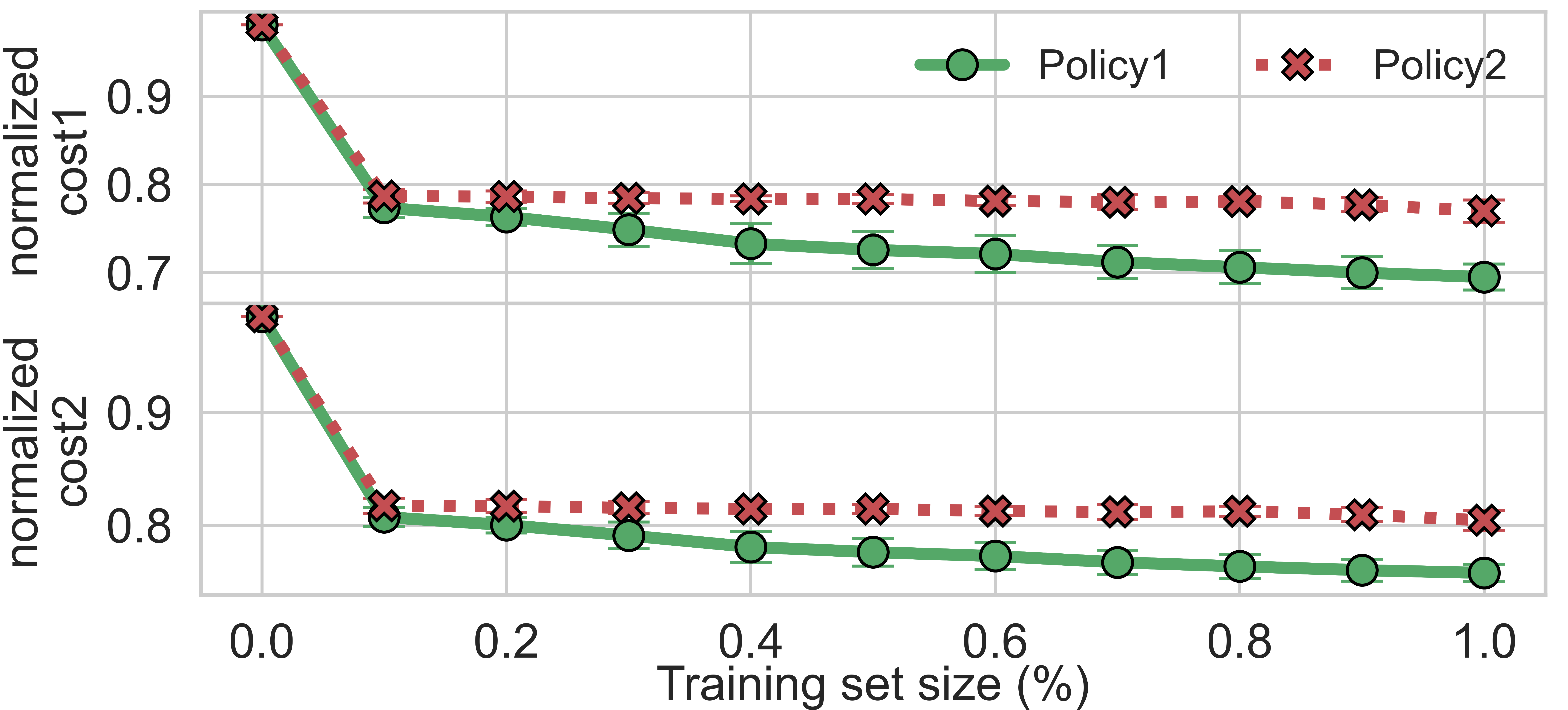
Figure 10. Benefit of Implicit Feedback: Policy1 trained on cost1 (more implicit feedback) performs better than Policy2 trained on cost2 (less implicit feedback), when evaluated on either cost metric.

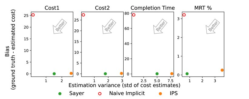
Figure 11. Counterfactual Evaluation of Policy2 (cost1, cost2, completion time, MRT meet rate) shows that it can be used to estimate different metrics than the one optimized by the policy.

Benefits of implicit exploration and feedback.  Figure 11 shows the counterfactual analysis error when using different approaches to evaluate Policy2’s performance. Each colored dot represents a different counterfactual estimator, but this time each box shows results for a different metric to evaluate (cost1, cost2, average VM creation time, and MRT meet rate). This shows that counterfactual evaluation can be used to evaluate multiple practically useful metrics, and not just the cost optimized by the policy. We can see that compared to Naive Implicit (using implicit feedback in a biased way) or $\mathtt{IPS}$ (unbiased but without implicit feedback), Sayer’s estimates are unbiased and have a standard deviation only half that of the $\mathtt{IPS}$ estimator ($10$ sec vs $20$ sec), showing the value of both implicit feedback (compared to $\mathtt{IPS}$) and exploration (compared to Naive Implicit).

Benefits of $\mathtt{Implicit}$ estimator.  Finally, Figure 12 shows results for policy training. Sayer outperforms policies trained by Naive Implicit, Direct Method, and $\mathtt{IPS}$, by 7.0%, 4.1%, and 4.1% respectively. To emphasize the value of our $\mathtt{Implicit}$ estimator, we also add a policy trained exclusively on exploration data (Exploration Only in Figure 12). Such an approach is unbiased, but it cannot use datapoints in which the data collection policy did not explore. This data reduction yields a policy that is 3.1% worse than Sayer, showing the value of our $\mathtt{Implicit}$ estimator leveraging every datapoint.

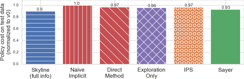
Figure 12. Sayer vs Baselines (data-driven simulation in Azure-Scale).

4.3.2. Online evaluation using live deployment

Finally, we show the end-to-end performance of Sayer in a live deployment of our prototype, compared to a Naive Implicit-trained policy, and the default policy (v0). Such an evaluation is not as simple as just deploying each policy in turn in the prototype, because the strong temporal patterns in creation times within Azure prevent comparisons between different time periods. Consequently, we add support for simultaneously deploying policies and randomly assigning each request to one of them, in an A/B/C test. This online testing framework allows Sayer and other policies to be deployed in the same environment and compared on live traffic at the same time. Both policies are initially trained using the same one week of full-feedback data. During the experiment, we replay our workload trace. Every 24 hours, each policy is retrained on a 1-week trailing window of data.

Figure 13 shows the performance of all three policies over time. At the beginning of the experiment, the Naive Implicit policy and Sayer are both trained on full-feedback data and perform equally well. Over time, the Naive Implicit-trained policy is retrained on biased data and performs unevenly. Sayer, on the other hand, consistently outperforms both the v0 and the Naive Implicit-trained policy.

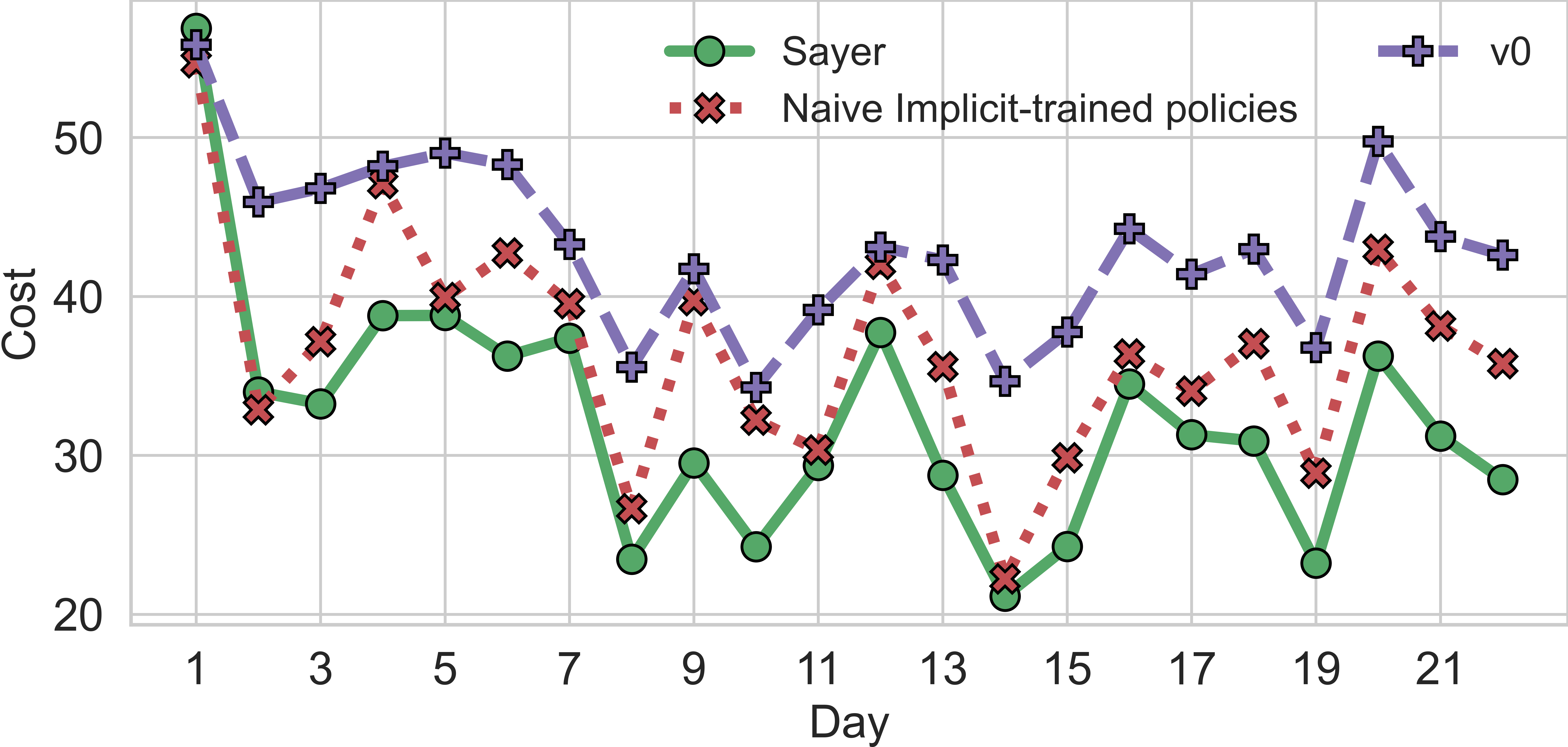
Figure 13. Live deployment (A/B/C tests). Randomly assigning each request to v0, Naive Implicit, or Sayer. Sayer consistently has the lowest cost.

5. Related work

Sayer attempts to bridge the gap between recent theoretical work on counterfactual evaluation and training in machine learning, and the challenge of evaluating and improving policies in systems. We focus on the most related work from both sides, and point the reader to §2.3 for a broader overview.

Counterfactual evaluation.  Sayer builds on Inverse Propensity Scoring (IPS) estimators, a classical technique from the 1950s (Horvitz and Thompson, 1952; Rotnitzky and Robins, 1995). Recent work extends IPS to contextual bandits (Dudik et al., 2011) and incorporates inherent structure for better data efficiency (Chu et al., 2011; Langford et al., 2008). These techniques have generally been applied to advertising and news articles (Bottou et al., 2013; Li et al., 2010; Joachims and Swaminathan, 2016). Sayer adapts these techniques to design a methodology for a broad class of system policies, and integrates it into their lifecycle.

Sayer leverages implicit feedback to boost the efficiency of counterfactual estimation. Implicit feedback has been studied using feedback graphs (Mannor and Shamir, 2011; Alon et al., 2013), but these works assume a fixed feedback graph and use it to optimize one policy online. In contrast, Sayer can counterfactually evaluate many policies, even when the feedback graph is outcome-dependent.

Sayer’s implicit feedback can be viewed as a variance reduction technique over IPS. Similarly, Doubly Robust (DR) estimators can also be used to reduce the variance of IPS, by combining a model-based predictor to “fill the gaps” when information is missing (Dudík et al., 2014). DR estimators are orthogonal to our contribution and can be applied to both Sayer and IPS.

Data-driven modeling in systems.  While most work in systems is evaluated on real testbeds or deployments, trace-driven evaluation is often used to evaluate new policies at scale (e.g., in server/path selection (Liu et al., 2016; Jiang et al., 2016a), video bitrate adaptation (Mao et al., 2017; Jiang et al., 2016b; Yin et al., 2015), and MapReduce scheduling (Kumar et al., 2016)). Data-driven models/simulators were developed for “what-if” analysis in specific systems settings (e.g., web service (Jiang et al., 2016c), CDN server selection (Tariq et al., 2008), end-to-end adaptation performance (Sruthi et al., 2020), and streaming video QoE modeling (Krishnan and Sitaraman, 2013)). Similar data-driven performance modeling is also used to predict the best configuration for a workload based on a few samples (Zhu et al., 2017). However, it is inherently difficult for these analyses to faithfully capture all relevant details (including confounding factors (Sruthi et al., 2020)) of a large-scale system (Floyd and Paxson, 2001), to simulate or build an analytical model that precisely predicts performance of any unobserved actions (Fu et al., 2021). In contrast, Sayer focuses on a class of decisions that exhibit independence properties, and uses tools from statistics/machine learning to enable unbiased evaluation without the need for modeling. Recently, (Lecuyer et al., 2017; Bartulovic et al., 2017) suggested the potential of such an approach, but fall short of addressing any systems challenges or developing any usable methodology.

RL and Online Learning in systems.  A closely related body of work uses (deep) reinforcement learning (e.g., (Tesauro, 2007; Mao et al., 2017; Erickson et al., 2010; Alipourfard et al., 2017; Van Aken et al., 2017; Li et al., 2019; Zhang et al., 2019)) or online learning (e.g., (Dong et al., 2015; Dong et al., 2018)) in systems optimization. It optimizes a single policy online by continuously interacting with the environment. Typically, the data collected by such a policy yields partial feedback that can only be used to evaluate policies that are similar to it. Sayer instead focuses on a class of techniques that enable unbiased counterfactual evaluation of any policy. Although our evaluation focuses on iterative model updates (which are common in production systems), we note that Sayer can also update a policy online as new data arrives.

6. Discussion

We applied Sayer’s counterfactual evaluation and training methodology to two systems: Azure-Health and Azure-Scale. These examples illustrate the value of counterfactual evaluation in systems, as well as the prevalence of implicit feedback in systems that make threshold decisions. They also illustrate the manual effort required to apply Sayer: specifically, Sayer relies on the system designer to define an event $E$ that captures the available implicit feedback, and compute its probability $P(E)$. Though nontrivial, defining this event follows naturally from reasoning about when cost feedback is known for the candidate policy’s action, based on the data collected by the deployed policy. For example in Azure-Health, the only case when feedback is not available is when the deployed policy’s action causes a timeout and the candidate policy chooses to wait even longer; $E$ is thus defined as the opposite of this event. After deriving $E$ for Azure-Health, it was relatively straightforward to do the same for Azure-Scale. Thus, in our experience, the manual effort required for a new application is reasonable.

As discussed in §3.1, Sayer applies to system decisions that satisfy certain independence properties (e.g., the same ones required by contextual bandits and $\mathtt{IPS}$). As such, it does not apply to system policies that maintain long-term state, or whose decisions interact in complex ways. Defining appropriate events and costs for individual actions in such settings is a challenging problem for reinforcement learning. It is an interesting open question if the ideas from Sayer, and in particular our techniques for leveraging implicit feedback, can be extended to more general RL to support these settings.

Sayer focuses on one-dimensional (single-parameter) decisions due to two limitations in our approach. The first is our reliance on existing RL techniques, which do not cope well with large or complex action spaces, mainly because they are unable to explore these spaces efficiently. A multi-dimensional action space grows exponentially in the number of dimensions: e.g., even a 2-parameter decision $(x\in\mathcal{X},y\in\mathcal{Y})$ where $|\mathcal{X}|=|\mathcal{Y}|=N$ has an action space of size $N^{2}$. The second limitation is that it is unclear if implicit feedback can be obtained in multi-dimensional decisions. For example, if we take the decision $(x,y)$, does that mean that we receive feedback for all actions $(\leq x,\leq y)$? Clearly this depends on the relationship between $x$ and $y$, which may be complex. Extending Sayer to multi-dimensional action spaces is an interesting direction for future work.

References

- (1)
- Alipourfard et al. (2017) Omid Alipourfard, Hongqiang Harry Liu, Jianshu Chen, Shivaram Venkataraman, Minlan Yu, and Ming Zhang. 2017. CherryPick: Adaptively Unearthing the Best Cloud Configurations for Big Data Analytics.. In NSDI, Vol. 2. 4–2.
- Alon et al. (2013) Noga Alon, NicolÃ2 Cesa-Bianchi, Claudio Gentile, and Yishay Mansour. 2013. From Bandits to Experts: A Tale of Domination and Independence. In Advances in Neural Information Processing Systems (NIPS). 1610–1618.
- Ananthanarayanan et al. (2013) Ganesh Ananthanarayanan, Ali Ghodsi, Scott Shenker, and Ion Stoica. 2013. Effective straggler mitigation: Attack of the clones. In 10th USENIX Symposium on Networked Systems Design and Implementation (NSDI 13). 185–198.
- Bartulovic et al. (2017) Mihovil Bartulovic, Junchen Jiang, Sivaraman Balakrishnan, Vyas Sekar, and Bruno Sinopoli. 2017. Biases in Data-Driven Networking, and What to Do About Them. In Proceedings of the 16th ACM Workshop on Hot Topics in Networks. ACM, 192–198.
- Bingham et al. (2018) Eli Bingham, Jonathan P. Chen, Martin Jankowiak, Fritz Obermeyer, Neeraj Pradhan, Theofanis Karaletsos, Rohit Singh, Paul Szerlip, Paul Horsfall, and Noah D. Goodman. 2018. Pyro: Deep Universal Probabilistic Programming. Journal of Machine Learning Research (2018).
- Bottou et al. (2013) Léon Bottou, Jonas Peters, Joaquin Quiñonero-Candela, Denis X Charles, D Max Chickering, Elon Portugaly, Dipankar Ray, Patrice Simard, and Ed Snelson. 2013. Counterfactual reasoning and learning systems: The example of computational advertising. The Journal of Machine Learning Research 14, 1 (2013), 3207–3260.
- Chu et al. (2011) Wei Chu, Lihong Li, Lev Reyzin, and Robert Schapire. 2011. Contextual bandits with linear payoff functions. In Proceedings of the Fourteenth International Conference on Artificial Intelligence and Statistics. 208–214.
- Dong et al. (2015) Mo Dong, Qingxi Li, Doron Zarchy, P Brighten Godfrey, and Michael Schapira. 2015. PCC: Re-architecting congestion control for consistent high performance. In Symposium on Networked Systems Design and Implementation (NSDI).
- Dong et al. (2018) Mo Dong, Tong Meng, Doron Zarchy, Engin Arslan, Yossi Gilad, Brighten Godfrey, and Michael Schapira. 2018. PCC vivace: Online-learning congestion control. In Symposium on Networked Systems Design and Implementation (NSDI).
- Dudík et al. (2014) Miroslav Dudík, Dumitru Erhan, John Langford, and Lihong Li. 2014. Doubly robust policy evaluation and optimization. Statist. Sci. (2014), 485–511.
- Dudik et al. (2011) Miroslav Dudik, Daniel Hsu, Satyen Kale, Nikos Karampatziakis, John Langford, Lev Reyzin, and Tong Zhang. 2011. Efficient Optimal Learning for Contextual Bandits. In Proceedings of the Twenty-Seventh Conference on Uncertainty in Artificial Intelligence.
- Efron (1979) B Efron. 1979. Bootstrap Methods: Another Look at the Jackknife. The Annals of Statistics (1979).
- Erickson et al. (2010) John Erickson, Madanlal Musuvathi, Sebastian Burckhardt, and Kirk Olynyk. 2010. Effective Data-Race Detection for the Kernel.. In OSDI, Vol. 10. 1–16.
- Floyd and Paxson (2001) Sally Floyd and Vern Paxson. 2001. Difficulties in simulating the Internet. IEEE/ACM Transactions on Networking (ToN) 9, 4 (2001), 392–403.
- Fu et al. (2021) Silvery Fu, Saurabh Gupta, Radhika Mittal, and Sylvia Ratnasamy. 2021. On the Use of ML for Blackbox System Performance Prediction.. In NSDI. 763–784.
- Horvitz and Thompson (1952) Daniel G Horvitz and Donovan J Thompson. 1952. A generalization of sampling without replacement from a finite universe. Journal of the American statistical Association 47, 260 (1952), 663–685.
- Imbens and Rubin (2015) Guido W. Imbens and Donald B. Rubin. 2015. Causal Inference for Statistics, Social, and Biomedical Sciences: An Introduction. Cambridge University Press.
- Jiang et al. (2016a) Junchen Jiang, Rajdeep Das, Ganesh Ananthanarayanan, Philip A Chou, Venkata Padmanabhan, Vyas Sekar, Esbjorn Dominique, Marcin Goliszewski, Dalibor Kukoleca, Renat Vafin, et al. 2016a. Via: Improving internet telephony call quality using predictive relay selection. In Proceedings of the 2016 ACM SIGCOMM Conference. 286–299.
- Jiang et al. (2016b) Junchen Jiang, Vyas Sekar, Henry Milner, Davis Shepherd, Ion Stoica, and Hui Zhang. 2016b. CFA: A Practical Prediction System for Video QoE Optimization.. In NSDI. 137–150.
- Jiang et al. (2016c) Yurong Jiang, Lenin Ravindranath Sivalingam, Suman Nath, and Ramesh Govindan. 2016c. WebPerf: Evaluating what-if scenarios for cloud-hosted web applications. In Proceedings of the 2016 ACM SIGCOMM Conference. ACM, 258–271.
- Joachims and Swaminathan (2016) Thorsten Joachims and Adith Swaminathan. 2016. Tutorial on Counterfactual Evaluation and Learning for Search, Recommendation and Ad Placement. http://www.cs.cornell.edu/~adith/CfactSIGIR2016/ A tutorial at SIGIR 2016.
- Klimovic et al. (2018) Ana Klimovic, Heiner Litz, and Christos Kozyrakis. 2018. Selecta: Heterogeneous cloud storage configuration for data analytics. In 2018 USENIX Annual Technical Conference (USENIXATC 18). 759–773.
- Kohavi and Longbotham (2015) Ron Kohavi and Roger Longbotham. 2015. Online Controlled Experiments and A/B Tests. In Encyclopedia of Machine Learning and Data Mining, Claude Sammut and Geoff Webb (Ed.). Springer. To appear.
- Kohavi et al. (2009) Ron Kohavi, Roger Longbotham, Dan Sommerfield, and Randal M. Henne. 2009. Controlled experiments on the web: survey and practical guide. Data Min. Knowl. Discov. (2009).
- Krishnan and Sitaraman (2013) S Shunmuga Krishnan and Ramesh K Sitaraman. 2013. Video stream quality impacts viewer behavior: inferring causality using quasi-experimental designs. IEEE/ACM Transactions on Networking 21, 6 (2013), 2001–2014.
- Kumar et al. (2016) Gautam Kumar, Ganesh Ananthanarayanan, Sylvia Ratnasamy, and Ion Stoica. 2016. Hold’em or fold’em?: aggregation queries under performance variations. In Proceedings of the Eleventh European Conference on Computer Systems. ACM, 7.
- Langford et al. (2008) John Langford, Alexander Strehl, and Jennifer Wortman. 2008. Exploration Scavenging. In Intl. Conf. on Machine Learning (ICML).
- Langford and Zhang (2007) John Langford and Tong Zhang. 2007. The Epoch-Greedy Algorithm for Contextual Multi-armed Bandits. In Advances in Neural Information Processing Systems (NIPS).
- Lecuyer et al. (2017) Mathias Lecuyer, Joshua Lockerman, Lamont Nelson, Siddhartha Sen, Amit Sharma, and Aleksandrs Slivkins. 2017. Harvesting Randomness to Optimize Distributed Systems. In Proceedings of the 16th ACM Workshop on Hot Topics in Networks. ACM, 178–184.
- Li et al. (2019) Guoliang Li, Xuanhe Zhou, Shifu Li, and Bo Gao. 2019. Qtune: A query-aware database tuning system with deep reinforcement learning. Proceedings of the VLDB Endowment 12, 12 (2019), 2118–2130.
- Li et al. (2010) Lihong Li, Wei Chu, John Langford, and Robert E Schapire. 2010. A contextual-bandit approach to personalized news article recommendation. In Proceedings of the 19th international conference on World wide web. ACM, 661–670.
- Liu et al. (2016) Hongqiang Harry Liu, Raajay Viswanathan, Matt Calder, Aditya Akella, Ratul Mahajan, Jitendra Padhye, and Ming Zhang. 2016. Efficiently Delivering Online Services over Integrated Infrastructure.. In NSDI, Vol. 1. 1.
- Mannor and Shamir (2011) Shie Mannor and Ohad Shamir. 2011. From Bandits to Experts: On the Value of Side-Observations. In Advances in Neural Information Processing Systems (NIPS). 684–692.
- Mao et al. (2017) Hongzi Mao, Ravi Netravali, and Mohammad Alizadeh. 2017. Neural adaptive video streaming with pensieve. In Proceedings of the Conference of the ACM Special Interest Group on Data Communication. ACM, 197–210.
- Peng et al. (2018) Yanghua Peng, Yixin Bao, Yangrui Chen, Chuan Wu, and Chuanxiong Guo. 2018. Optimus: an efficient dynamic resource scheduler for deep learning clusters. In Proceedings of the Thirteenth EuroSys Conference. 1–14.
- Rotnitzky and Robins (1995) Andrea Rotnitzky and James M Robins. 1995. Semiparametric regression estimation in the presence of dependent censoring. Biometrika 82, 4 (1995), 805–820.
- Sruthi et al. (2020) Panchapakesan C Sruthi, Sanjay Rao, and Bruno Ribeiro. 2020. Pitfalls of data-driven networking: A case study of latent causal confounders in video streaming. In Proceedings of the Workshop on Network Meets AI & ML. 42–47.
- Swaminathan et al. (2016) Adith Swaminathan, Akshay Krishnamurthy, Alekh Agarwal, Miroslav Dudík, John Langford 0001, Damien Jose, and Imed Zitouni. 2016. Off-policy evaluation for slate recommendation. CoRR (2016).
- Tariq et al. (2008) Mukarram Tariq, Amgad Zeitoun, Vytautas Valancius, Nick Feamster, and Mostafa Ammar. 2008. Answering what-if deployment and configuration questions with wise. In ACM SIGCOMM Computer Communication Review, Vol. 38. ACM, 99–110.
- Tesauro (2007) Gerald Tesauro. 2007. Reinforcement learning in autonomic computing: A manifesto and case studies. IEEE Internet Computing 11, 1 (2007).
- Van Aken et al. (2017) Dana Van Aken, Andrew Pavlo, Geoffrey J Gordon, and Bohan Zhang. 2017. Automatic database management system tuning through large-scale machine learning. In Proceedings of the 2017 ACM International Conference on Management of Data. 1009–1024.
- Venkataraman et al. (2016) Shivaram Venkataraman, Zongheng Yang, Michael Franklin, Benjamin Recht, and Ion Stoica. 2016. Ernest: Efficient performance prediction for large-scale advanced analytics. In 13th USENIX Symposium on Networked Systems Design and Implementation (NSDI 16). 363–378.
- Vowpal Wabbit ([n.d.]) Vowpal Wabbit [n.d.]. Vowpal Wabbit (Fast Learning). http://hunch.net/~vw/.
- Yadwadkar et al. (2017) Neeraja J Yadwadkar, Bharath Hariharan, Joseph E Gonzalez, Burton Smith, and Randy H Katz. 2017. Selecting the best vm across multiple public clouds: A data-driven performance modeling approach. In Proceedings of the 2017 Symposium on Cloud Computing. 452–465.
- Yin et al. (2015) Xiaoqi Yin, Abhishek Jindal, Vyas Sekar, and Bruno Sinopoli. 2015. A control-theoretic approach for dynamic adaptive video streaming over HTTP. In ACM SIGCOMM Computer Communication Review, Vol. 45. ACM, 325–338.
- Zaharia et al. (2008) Matei Zaharia, Andy Konwinski, Anthony D Joseph, Randy H Katz, and Ion Stoica. 2008. Improving MapReduce performance in heterogeneous environments.. In Osdi, Vol. 8. 7.
- Zhang et al. (2019) Ji Zhang, Yu Liu, Ke Zhou, Guoliang Li, Zhili Xiao, Bin Cheng, Jiashu Xing, Yangtao Wang, Tianheng Cheng, Li Liu, et al. 2019. An end-to-end automatic cloud database tuning system using deep reinforcement learning. In Proceedings of the 2019 International Conference on Management of Data. 415–432.
- Zhu et al. (2017) Yuqing Zhu, Jianxun Liu, Mengying Guo, Yungang Bao, Wenlong Ma, Zhuoyue Liu, Kunpeng Song, and Yingchun Yang. 2017. Bestconfig: tapping the performance potential of systems via automatic configuration tuning. In Proceedings of the 2017 Symposium on Cloud Computing. 338–350.